Embed Size (px)
Citation preview
Loughborough UniversityInstitutional Repository
Finite element modelling ofmechanical properties of
polymer composites
This item was submitted to Loughborough University's Institutional Repositoryby the/an author.
Additional Information:
• A Doctoral Thesis. Submitted in partial fulfillment of the requirementsfor the award of Doctor of Philosophy of Loughborough University.
Metadata Record: https://dspace.lboro.ac.uk/2134/7075
Publisher: c© Elaheh Ghassemieh
Please cite the published version.

This item is held in Loughborough University’s Institutional Repository (https://dspace.lboro.ac.uk/) and was harvested from the British Library’s EThOS service (http://www.ethos.bl.uk/). It is made available under the
following Creative Commons Licence conditions.
For the full text of this licence, please go to: http://creativecommons.org/licenses/by-nc-nd/2.5/
Finite Element Modelling Of Mechanical Properties
Of Polymer Composites
By
ELAHEH GHASSEMIEH
A Doctoral Thesis
. ý,.,:... sv. x-..,... ý.. r,. ýa.. », _
Submitted in partial fulJlment of the requirements For the award of Doctor Of Philosophy
By Loughborough University ý ý. 'Ti: #CH4 .r.
ý.;. . vw. umaq. f'. *d. s'Yfa. raaa.... -. w . ̀. xntMf ýrw
II Wa°IF+; AG. } ,., -a ,. -,. ., 1r "1 -r _. ý
t-,
December 1998

To those whose love kept my heart warm and encouraged me all through my life, during the period of this study
and in near or far,
especially my dear mother Parichehr and my father Mehdi

Acknowledgements
Hereby I would like to thank my supervisor, Dr. V. Nassehi, for his
assistance and advice during the course of this research and I wish to
showmygratitude to all the members of staff and students in the Chemical Engineering Department of Loughborough University who accompanied me allover the way. Ilearned a lot from them and I
enjoyed being with them. A door to a new world was opened to me, an experience that will
always be remembered.
ABSTRACT
Polymeric composites are used widely in modern industry. The prediction
of mechanical behaviour of these material under different loadings is
therefore of vital importance in many applications. Mathematical
modelling offers a robust and cost effective method to satisfy this
objective. In this project a comprehensive finite element model for
particulate and fibre reinforced composites is developed.
The most significant features of this model are:
" The inclusion of slip boundary conditions.
" The inclusion of flux terms across the inter-phase boundaries to take
the discontinuity of the material properties into account in the model.
" The use of penalty method in conjunction with Stokes flow equations
which allow the application of the developed model to solid elasticity
analysis as well as creeping viscous flows.
The predictions of this model are compared with available theoretical
models and experimental data. These comparisons show that the
developed model yields accurate and reliable data for composite
deformation.
TABLE OF CONTENTS
Chapter One
INTRODUCTION ..................................................................................................... I
Chapter Two
LITERATURE REVIEW .......................................................................................... 8
2.1 INTRODUCTION ........................................................................................................ 8
2.2 TYPES OF COMPOSITES ........................................................................................... 9
2.2.1 Polymeric composites filled with fibres .................................................................................. 9
2.2.2 Polymeric composites filled with particulate fillers .............................................................. 10
2.3 MECHANICAL PROPERTIES OF POLYMERIC COMPOSITES ........................ 10 2.3.1 Mechanical properties of unfilled polymers .........................................................................
11 2.3.2 Mechanical properties of particulate filled polymers ...........................................................
12 2.3.3 Non-linear behaviour of polymeric composites ....................................................................
14
2.4 THEORETICAL MODELS FOR DETERMINATION OF THE MODULUS OF COMPOSITES .................................................................................................................. 15
2.4.1 Theories of rigid inclusions in a non-rigid matrix ................................................................ 16 2.4.1.1 Einstein equation and its modifications ..................................................................... 16 2.4.1.2 The Kerner equation and its modifications ................................................................ 18
2.4.2 Theories of non-rigid inclusions in a non-rigid matrix ........................................................ 19 2.4.2.1 Series and parallel models ......................................................................................... 20 2.4.2.2 The Hashin and Shtrikman model ............................................................................. 20 2.4.2.3 The Hirsch model ..................................................................................................... 21 2.4.2.4 The Takayanagi model .............................................................................................. 22 2.4.2.5 The Counto model .................................................................................................... 22
2.4.3 Llimitations of the theoretical models .................................................................................. 23
2.5 MICROMECHANICAL ANALYSIS OF POLYMERIC COMPOSITES .............. 24 2.5.1 Qualitative description of the microstructure ...................................................................... 25
2.5.1.1 Geometric models ..................................................................................................... 25
I
2.5.1.2 Geometric model used in finite element modelling of composites ................................ 27
2.5.1.3 Structural descriptors ................................................................................................ 28
2.5.1.4 Size Of Particles ........................................................................................................ 30
2.5.2 Interface-adhesion ............................................................................................................. 30
2.6. FINITE ELEMENT MODELLING OF THE MECHANICAL PROPERTIES OF COMPOSITES ..................................................................................................................
31 2.6.1 Finite element methods based on variational principles .......................................................
31 2.6.1.1 Displacement method .................................................................................................
32 2.6.2 Least-square and Weighted residual method ........................................................................
37 2.6.2.1 A brief outline of the Galerkin method ........................................................................
38
Chapter Three
DEVELOPMENT OF THE PREDICTIVE MODEL ............................................. 39
3.1 MODEL EQUATIONS .............................................................................................. 39
3.1.1 Axisymmetric stress condition ............................................................................................ 39
3.1.2 Plain strain condition ......................................................................................................... 44
3.2 MODEL GEOMETRY AND BOUNDARY CONDITIONS ................................... 47
3.2.1 Modelling of the particulate filled composites ..................................................................... 47
3.2.2 Fibre reinforced composite ................................................................................................. 50
3.2.1.1 Tensile loading .......................................................................................................... 51
3.2.2.2 Shear loading ............................................................................................................. 52
3.2.3 Slip boundary conditions .................................................................................................... 52
3.3 CALCULATIONS .............................................. ......................................................... 55
3.3.1 Composite modulus of elasticity and Poisson's ratio ........................................................... 55
3.3.2 Composite strength .............................................................................................................. 56
3.3.3 Stress calculations( Variational recovery) ........................................................................... 56
Chapter Four
RESULTS AND DISCUSSION .............................................................................. 60
4.1 MODULUS .................................................................................................................. 63
4.1.1 Equal Stress and Equal Strain Bounds ................................................................................. 63
4.1.2 Model predictions and experimental results ......................................................................... 67
4.1.2.1 Agglomeration ............................................................................................................ 67
4.1.2.2 Dewetting ................................................................................................................... 67
4.1.2.3 Adhesion and bonding ................................................................................................
69 4.1.2.4 Arrangement ..............................................................................................................
69 4.1.2.5 Filler particle shape ....................................................................................................
71 4.2.3. Boundary conditions used in the finite element model ........................................................
72
11
4.2 COMPOSITES FILLED WITH RIGID PARTICLES ............................................. 73 4.2.1. Young's modulus ............................................................................................................... 73 4.2.2 Stress distribution ................................................................................................................ 73
4.2.2.1 Concentration of direct stress ...................................................................................... 73 4.2.2.2 Stresses at the interface ............................................................................................... 76
4.2.3. Compression ...................................................................................................................... 78 4.2.4 Concentration of yield stress ................................................................................................ 78 4.2.5 Fracture behaviour ............................................................................................................... 83
4.3 COMPOSITES FILLED WITH DEBONDED RIGID PARTICLES ..................... 90 4.3.1 Boundary conditions at the interface ...................................................................................
90 4.3.2 Displacement ......................................................................................................................
92 4.3.3 Interfacial stresses ...............................................................................................................
92 4.3.4 Slipping of the particle at part of the interface ...................................................................
102 4.3.5 Strength ............................................................................................................................
102
4.4 COMPOSITES FILLED WITH SOFT PARTICLES ............................................ 105
4.4.1 Material properties ............................................................................................................ 105
4.4.2 Young's modulus ............................................................................................................. 105
4.4.3 Stress distribution .............................................................................................................. 109
4.4.3.1 Concentration of direct stress .................................................................................... 109
4.4.3.2 Stresses at the interface ............................................................................................. 114
4.4.3.3 Hydrostatic stress in the rubber particle .................................................................... 114
4.4.3.4 Concentration of yield stress ..................................................................................... 116
4.4.3.5 Stresses in the matrix ............................................................................................... 116
4.4.4 Fracture behaviour ............................................................................................................ 118
4.5 FIBRE REINFORCED COMPOSITES ................................................................... 123
4.5.1 Transverse tensile loading ................................................................................................. 123
4.5.1.1 Modulus ................................................................................................................... 123
4.5.1.2 Concentration of applied stress ................................................................................ 123
4.5.1.3 Stresses at interface ................................................................................................... 128
4.5.1.4 Fracture strength ...................................................................................................... 130
4.5.2 Transverse shear loading .................................................................................................. 134
4.5.2.1 Modulus .................................................................................................................. 134
4.5.2.2 Stress distribution and strength ................................................................................. 134
4.6 SHORT FIBRE REINFORCED COMPOSITES ................................................... 139 4.6.1 Modulus ............................................................................................................................
139 4.6.2 Stress distribution .............................................................................................................. 147
4.6.2.1 Interfacial shear stress distribution ............................................................................ 147 4.6.2.2 Interfacial tensile stress distribution
......................................................................... 147 4.6.2.3 Tensile stress in the fibre .......................................................................................... 147
4.6.3 Critical length ................................................................................................................... 150 4.6.4 Strength of short fibre composites ...................................................................................... 154
UI
Chapter Five
CONCLUSION ................................................................................................................. 159
5.1 CONCLUSIONS Of THE PRESENT WORK ........................................................ 159 5.1.1 Modulus of particulate filled composites ............................................................................
159 5.1.2 composites filled with hard particles ..................................................................................
160 5.1.3 Composite filled with partially bonded particles ................................................................
162 5.1.4 Composite filled with soft particles ....................................................................................
163 5.1.5 Composites reinforced with continuous fibres ....................................................................
165 5.1.6 Composites reinforced with short fibres .............................................................................
167
5.2 SUGGESTIONS FOR FURTHER WORK ............................................................ 169
IV
Chapter One
INTRODUCTION
Polymeric composites are amongst the most important new material resources. This is
because of the relative low cost of manufacturing of these materials and the possibility
of obtaining improved and unique properties from them. The bulk properties of
polymeric composites obviously depend on their microstructure. Therefore the
composite properties and their behaviour should be assessed and analysed considering
microstructural responses of composites to external loading and conditions.
The main objectives of this project have been the analysis of the micromechanical
behaviour of different types of polymeric composites using mathematical modelling.
We have considered continuous fibre reinforced composite, short fibre reinforced
composite and composites with hard or soft particles.
To understand the mechanical behaviour of composites, the mechanical behaviour of
the constituent materials and the interactions of these constituents should be
investigated.
Mathematical modelling offers a powerful prediction tool to carry out such investigation. In recent years a number of mathematical models for the microstructural behaviour of composites have been proposed. Most of these models are formulated in
terms of mathematical equations, which cannot be solved analytically. Therefore in
most cases the use of a numerical technique for the quantitative analysis of composite behaviour is required.
Chanter One Introduction
Finite element method combines robustness with flexibility and hence it is the method
of choice in most applications. In this project we have considered the finite element
schemes based on the `displacement method' and the `weighted residual method'. It is
especially important to note that using the latter method a mathematical model for the
microstructural analysis of composites can be developed which is based on equations
similar to the fundamental equations of fluid dynamics. This approach has the
advantage of using a single model for the analysis of composites in liquid or solid state.
This thesis consists of five chapters. The introductory chapter describes the outline of
the thesis and includes a summary of the properties of various composites investigated
in the present work. In chapter two a thorough literature survey is given and the
background of the present project is presented. In chapter three the development of the
working equations of the model and the domain geometry are described. This chapter
also includes explanation regarding the finite element mesh, the boundary conditions
and the postprocessing calculations used. Chapter four is devoted to the computational
results and discussion and the comparison with the available experimental data and the
results generated by other models. Chapter four consists of the following sections:
In section one of this chapter the most important bulk property of composites, the
modulus is studied. The effect of model assumptions and boundary conditions on the
results obtained are discussed.
In section two the mechanical behaviour of epoxy resin filled with hard glass particles
is studied as a typical composite filled with rigid particles. The addition of rigid
particles to epoxy resins can result in a significant improvement in the properties of the
resin and a considerable reduction in cost. There is invariably an increase in the
stiffness of the resin but the effect of the particles upon the fracture behaviour is
complex. The fracture behaviour of multiphase polymers has been reviewed and there
has been considerable interest over the years in crack propagation in brittle materials
reinforced with rigid filler particles. It is found that, in general, both the critical stress
intensity factor and fracture energy increase with the addition of rigid particles, at least
for low volume fractions of filler. The most generally accepted explanation of this
2
Chapter One Introduction
behaviour, using the analogy of a dislocation moving through a crystal, is that a crack
in a body possesses "line tension" and that when it meets an array of a impenetrable
obstacles it becomes pinned. In order to move past the obstacles the crack would have
to bow out and this leads to an increase in fracture energy. The fracture energy reaches
a maximum at a particular value of filler volume fraction and then falls with the further
addition of particles, implying that there may be another mechanism which competes
with crack front pinning at high volume fractions of filler.
Particulate filled composites are used in applications ranging from everyday usage, like
automobile tires, to specific, such as solid rocket propellants. These materials exhibit
interesting failure properties. Phenomena such as cavitation (the appearance of voids)
and debonding (adhesive failure between matrix and filler particles) lead to gross
nonlinearities in their stress-strain behaviour. Particulate composites subjected to large
strains generally exhibit large degrees of debonding. The parameters that affect this
failure include particle size, filler concentration, surface treatments, matrix and filler
properties, superimposed pressure, and strain rate. Debonding of filler particles
appears to be the dominant factor influencing both stress-strain and volumetric
behaviour of particulate materials.
In section three the stress field in a composite with partially or fully debonded rigid
particles is analysed. Bond degradation is often a critical factor in determining the
ultimate strength of a composite material, as well as its fatigue resistance, impact
resistance, and other important properties. The strength of the bonding between filler
and matrix plays a major role in the ability of the composite to bridge cracks or deflect
cracks along the interface and, thereby, contribute to composite fracture toughness.
For such fracture toughening to occur, the filler matrix interface must exhibit just the
right degree of bonding. If the bonding is too strong, the composite behaves like a
monolithic material and cracks propagate through the material generally resulting in
brittle fracture.
3
Chapter One Introduction
Improving adhesion at the interface increases the fracture strength of the composite , it
is not entirely clear how this affects crack propagation. There have been reports of
improving adhesion at the interface both increasing and decreasing the fracture energy,
for crack propagation in particle reinforced composites.
With good adhesion it is found that the fracture strength of the composites is
approximately the same as that of the unfilled matrices. On the other hand, with no
surface pretreatments, or release agents, applied to the particles the strength decreases
with increasing volume fractions of filler particles.
In the fourth section of chapter four the effects of adding rubbery particles on the
mechanical characteristic of a matrix material such as epoxy resin are studied. The
improvement of the impact properties of polymers is possible through incorporation of
rubbery phase domains into a brittle polymer matrix. The increase in the toughness of
glassy polymers with addition of rubber particles is believed to be due to induced wide-
spread energy absorbing deformation processes, such as crazing and shear yielding, in
the matrix material during fracture. Shear yielding is important; firstly, it is the factor
which limits the strength of the composite if brittle fracture can be suppressed. A
composite must have a high yield stress in order to be strong and if bulk, homogeneous
yielding does occur the polymer is likely to be tough. Secondly, recent evidence
suggests that shear yielding, in the form of microshear bands, plays a key role in the
initiation of cracks. Shear yielding and crazing, both involve localised, or
inhomogeneous, plastic deformation of the material which arises from strain softening
and geometric considerations. The difference between the mechanisms is that shear
yielding occurs essentially at constant volume whereas crazing occurs with an increase
in volume. Thus, unlike shear yielding, crazing is a cavitation process in which the
initiation step requires the presence of a dilatational component to the stress tensor and
may be inhibited by applying hydrostatic pressure but enhanced in the presence of
triaxial tensile stresses.
A craze is initiated when an applied tensile stress causes microvoids to nucleate at
points of high stress concentrations in polymer. These microvoids are created by
4
Chapter One Introduction
scratches, flaws, cracks, dust particles, molecular heterogeneities. In general the
microvoids develop in a plane perpendicular to the maximum principal stress but do
not coalesce to form a true crack. Thus a microvoid is capable of transmitting loads
across its faces. However, when cracks do initiate and grow they do so by means of
the breakdown of the fibrillar structure in a craze. The importance of crazing is that it
is frequently a precursor to brittle fracture. This is because, although considerable
plastic deformation and local energy adsorption are involved in craze initiation, growth
and breakdown, this micromechanism is often highly localised and confined to a very
small volume of the material. However, it should be recognised that if stable crazes
can be initiated in a comparatively large volume of the polymer, i. e. a multiple
deformation mechanism is induced, then such multiple crazing may lead to a tough,
and possibly even a ductile, material response.
Crazes are formed at the rubber particles whereas shear yielding takes place between
the modifier particles.
The rubber inclusions cause a local stress magnification in the matrix material
immediately surrounding the inclusions. This local stress magnification is believed to
initiate crazing and shear yielding. A great deal of controversy still exists on the
nature of the toughening mechanisms. Much of the dispute surrounds the issues of
whether the rubber or the matrix absorbs most of the energy and whether the matrix
undergoes massive crazing or simple voiding. Presumably, once the mechanisms
responsible for the increased toughness are clearly identified, then the material
parameters responsible for these mechanisms can be enhanced or modified to produce
an optimal combination of properties.
The behaviour of the continuous fibre reinforced composites under tensile and shear
loading is studied in section five of chapter four. High specific strength and stiffness
properties of fibre reinforced composite materials have resulted in their widespread use
in load bearing structures. These structures have complex geometries and are often
subjected to multiaxial loadings. Monolithic material mechanical behaviour can be
adequately described by a limited number of material properties and strength criteria as
these materials present simple failure modes under different loading and boundary
5
Chapter One Introduction
conditions. Strength characterisation of composite laminate structures is more difficult
to estimate because of the variety of failure modes and failure mode interactions. For a
continuous fibre reinforced composite, the strength of the composite is derived from
the strength of the fibres, but this strength is highly directional in nature. The
longitudinal strength of the continuous fibre reinforced composites is much greater
than the transverse strength. The compressive strengths associated with these
directions may be different from the corresponding tensile strengths.
Failure of composite materials are determined not only by their internal properties such
as properties of constituents and microstructural parameters but also by external
conditions such as geometric variables, type of loading and boundary conditions.
Critical failure modes for each composite material system under various loading
conditions must be identified and a failure criterion should be established for each
failure mode.
Finally the last section of chapter four presents the results of the analysis of the short
fibre reinforced composites. Short fibre reinforced composites are not as strong or as
stiff as continuous fibre reinforced composites and are not likely to be used in critical
structural applications. However, short fibre composites do have several attractive
characteristics that make them worthy of consideration for other applications. For
example, in components having complex geometrical contours, continuous fibres may
not be of practical use because they may not conform to the desired shape without
being damaged or distorted from the desired pattern. On the other hand, short fibres
can be easily mixed with the liquid matrix resin, and the resin/fibre mixture can be
injection or compression moulded to produce parts having complex shapes. Such
processing methods are also fast and inexpensive, which makes them very attractive for
high volume applications. Composites having randomly oriented short fibre
reinforcement are nearly isotropic, whereas unidirectional continuous fibre composites
are highly anisotropic. In many applications the advantages of low cost, ease of
fabricating geometrically complex parts, and isotropic behaviour are enough to make
short fibre composites the material of choice.
6
Chanter One Introduction
Since the elastic modulus of the fibre is typically much larger than that of the matrix, the axial elastic displacements of the two components can be very different. In order to
rationalise the design of reinforced materials, it is thus of primary importance to have a detailed knowledge of stress distribution induced by the applied load. Indeed, when discontinuous fibres are used, the attainment of good mechanical properties depends
critically upon the efficiency of stress transfer between matrix and the fibres. That
efficiency is often characterised by the critical length required of the fibre to build up a
maximum stress equal to that of an infinitely long fibre.
The effective properties of fibre reinforced composites strongly depend on the
geometrical arrangement of the fibres within the matrix. This arrangement is
characterised by the volume fraction of fibres, the fibre aspect ratio and the fibre
spacing parameter. Analytical equations for the variation of stress along discontinuous
fibres in a cylindrically symmetrical model have been derived by Cox. In this approach
the adhesion across the end face of the fibres is neglected and the local stress
concentration effects near fibre ends have not been taken into account. The importance
of these assumptions has been demonstrated by finite element approaches.
The overall conclusions of the present project are discussed in chapter five. The list of
references quoted in the text is included at the end of the thesis.
The main objectives of this project can be summarised as:
Developing a model to predict the mechanical properties of polymer composite
Developing a code that can be used for studying the behaviour of the polymer
composites in the both solid and liquid states.
Including the boundary line integral terms in the model and investigating the effect
of that on the final results of the computations for different shape of the fillers and
composites.
7
Chapter One Introduction
Imposing the slip boundary condition at the interface of the filler and matrix in
order to simulate the level of adhesion at the boundary of a debonded filler particle.
Applying the developed model for different types of composites such as
composites filled with hard particles or soft particles, composite reinforced with
continuous or short fibres. Using the proper geometry model and boundary
condition for each case. Validating the results of the computation by comparing
with experimental data and other well established model in each case in order to
evaluate our model in qualitative and quantitative analysis.
ý
Chapter Two
LITERATURE REVIEW
2.1 INTRODUCTION
A composite material is a combination of at least two chemically distinct materials
with a distinct interface separating the components. Composites can offer a
combination of properties and a diversity of applications unobtainable with metals,
ceramics or polymers alone. Composites are also used when it is necessary to
substitute the traditional materials. Substitution can be the result of legislation,
performance improvement, cost reduction and expansion of product demand. For
example the trend of legislation on minor impact damage has provided motivation for
widespread substitution of plastics with metals in automobile bumpers. Improvement
of mechanical properties such as load bearing and transfer, creep, fatigue strength and high temperature strength is also regarded as an important reason for designing and
manufacturing of polymer composites. The enhancement of heat, abrasion, oxidation,
corrosion and wear resistance which can protect the objects confronting
environmental attacks is another reason for the increased use of composite materials. Improved electrical, magnetic and thermal conductivity properties can also be
considered as objectives of the design of composite materials.
q CIL
Chapter Two
2.2 TYPES OF COMPOSITES
Literature Review
In polymeric composites the base or matrix is a polymer and the filler is an inorganic
or organic material in either fibre or particulate form.
The properties of an advanced composite are shaped not only by the kind of matrix
and reinforcing materials it contains but also by another factor which is distinct from
composition. This factor is the geometry of reinforcement. Geometrically, composites
can be grouped roughly by the shape of the reinforcing elements as particulate,
continuous fibre or short fibre composites.
2.2.1 Polymeric composites filled with fibres
Addition of fibres to a polymer matrix enhances its stiffness, strength, hardness,
abrasion resistance, heat deflection temperature and lubricity while reducing its
shrinkage and creep. The fibre aspect ratio (i. e. the ratio of the characteristic length L
to the characteristic diameter D of a typical fibre) and the orientation of fibres have
profound influence on the properties of the composites. The most effective
reinforcing fillers are fibres which intrinsically have a high elastic modulus and tensile
strength. A superior composite is a material which can effectively transfer the applied
load to the fibres.
Fibres can be made of organic material such as: Cellulose, Wood, Carbon / Graphite,
Nylons and Polyester. At the present time however, for reasons of constitutional
strength, stiffness, thermal stability, and sometimes cost, inorganic fibres are the most
important reinforcement materials which are compounded with polymers. Recent
developments in high modulus and thermally-resistant organic fibres are creating
interest, especially where light weight materials are needed as in aerospace
applications. Inorganic materials such as Asbestos, Glass, Boron, Ceramic, Metal
filaments are commonly used in the production of fibres. Similar to organic fibres,
these are produced using both natural and synthetic raw materials.
2.2.2 Polymeric composites filled with particulate fillers
This kind of filler embraces not only fillers with regular shapes, such as spheres, but
also many of irregular shapes possibly having extensive convolution and porosity in
9
Chapter Two Literature Review
addition. However, the use of these types of fillers does not improve the ultimate tensile strength of the composites. In fact the tensile, flexural and impact strength of
these composites are lowered, especially at higher filler contents. On the other hand
hardness, heat deflection temperature and surface finish of particulate filled
composites may be enhanced and their stiffness is mainly improved. Thermal
expansion, mold shrinkage extendibility and creep are reduced too. The main
advantage of using these fillers is that regardless of the bonding efficiency between
particulate filler and matrix, the properties remain consistent. In addition the elastic
modulus and the heat distortion temperature increases while structural strength
decreases.
Wood flour, Cork, Nutshell, Starch, Polymers, Carbon and Protein are some of the
commonly used organic particulate fillers.
Despite limited thermal stability, organic fillers have' an advantage of being of low
density and many have a valuable role as a cheap extender for the more expensive
base polymer, as well as providing some incidental property such as reduction of
mould shrinkage which is important in polymer processing.
Glass, Calcium carbonate, Alumina, Metal oxides, Silica and Metal powder are
examples of the inorganic materials which are used as particulate fillers.
This class of fillers constitutes the more important group of particulate fillers in view
of their low price and ready availability. Thus providing a basis for reducing the cost
of moulded articles made with particulate filled composites without too much loss, if
any, of desired properties (Sheldon, 1982).
2.3 MECHANICAL PROPERTIES OF POLYMERIC COMPOSITES
In many respects the mechanical properties of different polymers are their most
important characteristics. Since whatever may be the reason for the choice of a
particular polymer for an application, (whether it be thermal, electrical or even
aesthetic grounds), it must have certain characteristics of shape, rigidity and strength. For polymer composites, improvement of mechanical behaviour is a prime
requirement. Since by definition the polymer constitutes the continuous phase, the
filler acts essentially through a modification of the intrinsic mechanical properties of
10
Chapter Two Literature Review
the polymer. Factors such as concentration, type, shape and geometrical arrangement
of the filler within the matrix are the main contributors to the modification of the
mechanical properties of polymer composites.
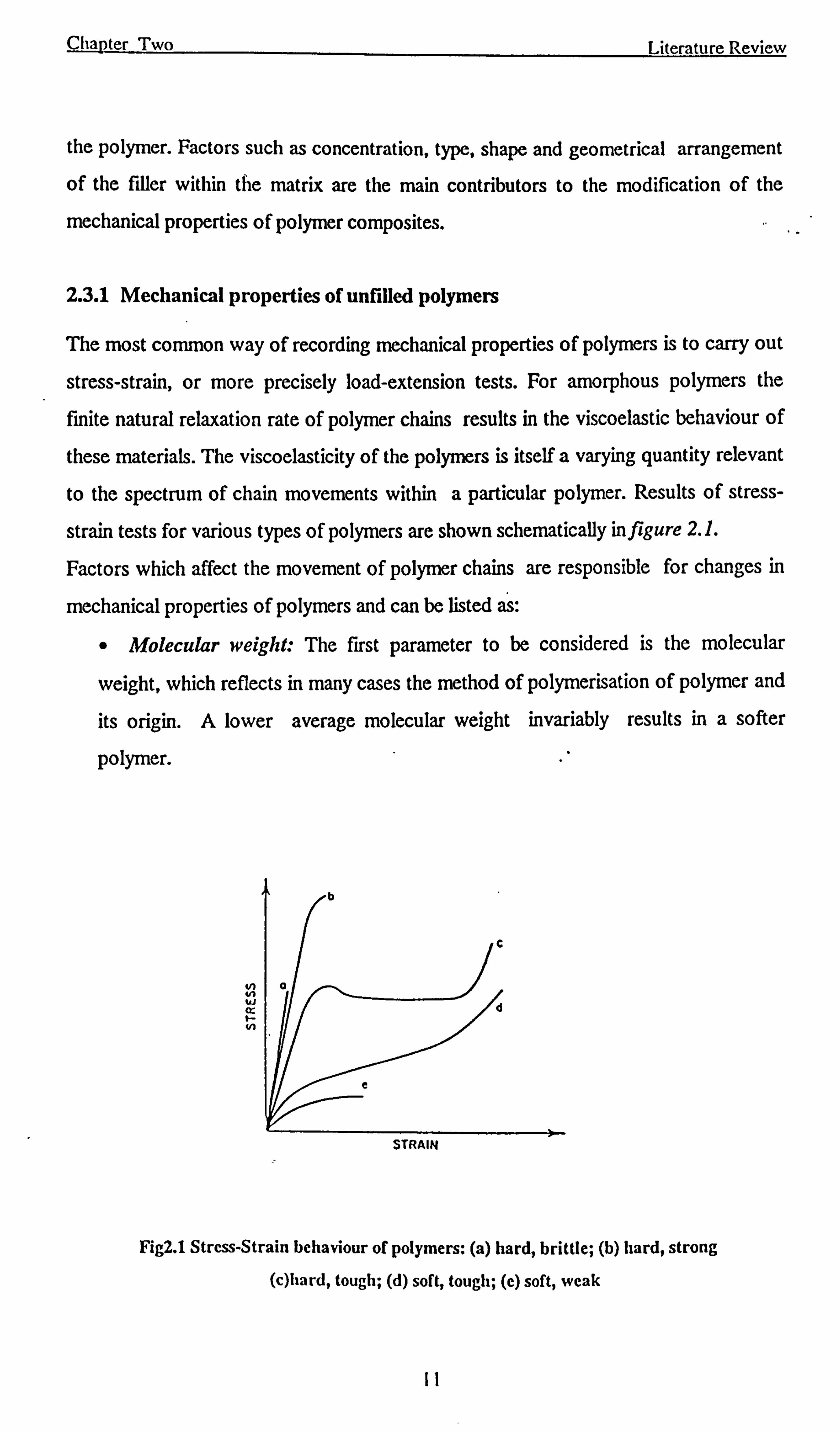
2.3.1 Mechanical properties of unfilled polymers
The most common way of recording mechanical properties of polymers is to carry out
stress-strain, or more precisely load-extension tests. For amorphous polymers the
finite natural relaxation rate of polymer chains results in the viscoelastic behaviour of
these materials. The viscoelasticity of the polymers is itself a varying quantity relevant
to the spectrum of chain movements within a particular polymer. Results of stress-
strain tests for various types of polymers are shown schematically in figure 2.1.
Factors which affect the movement of polymer chains are responsible for changes in
mechanical properties of polymers and can be listed as:
" Molecular weight: The first parameter to be considered is the molecular
weight, which reflects in many cases the method of polymerisation of polymer and
its origin. A lower average molecular weight invariably results in a softer
polymer.
N fn ui cr F- N
STRAIN
Fig2.1 Stress-Strain behaviour of polymers: (a) hard, brittle; (b) hard, strong
(c)hard, tough; (d) soft, tough; (e) soft, weak
II
Chapter Two Literature Review
" Branching or cross-linking: Any cross-linking between polymer chains will
push up the transition temperature.
" Crystallinity: Crystallinity in the polymer presents an intermediate case, with
some of rigidity being retained through the stabilising effect of the crystalline
regions which themselves only fail when the melting point is reached. The overall
relaxation behaviour is affected by the restricted movement of those chains which
are in crystalline regions, and a new type of time dependent response can arise
through structural slippage within these regions.
" Impurities: The presence of impurities or low molecular weight additives such
as moisture or organic liquids, will produce a softening as well as a weakening
effect.
" Temperature: It is not exceptional for a polymer to transverse all five of the
above classes of mechanical properties in a temperature range of no more than
hundred degrees. For an amorphous polymer, the biggest transition in mechanical
properties takes place at the glass transition temperature.
" Strain rate: The response of a polymer is affected by the rate of applying
strain especially just above the glass transition temperature, when an increase of
deformation rate causes an increase in apparent modulus and also usually gives rise
to a more brittle-like failure of the polymer.
2.3.2 Mechanical properties of particulate filled polymers
A filler may be primarily used as an inexpensive extender, pigment or UV stabiliser. The produced composite must still have suitable mechanical properties for its intended
application.
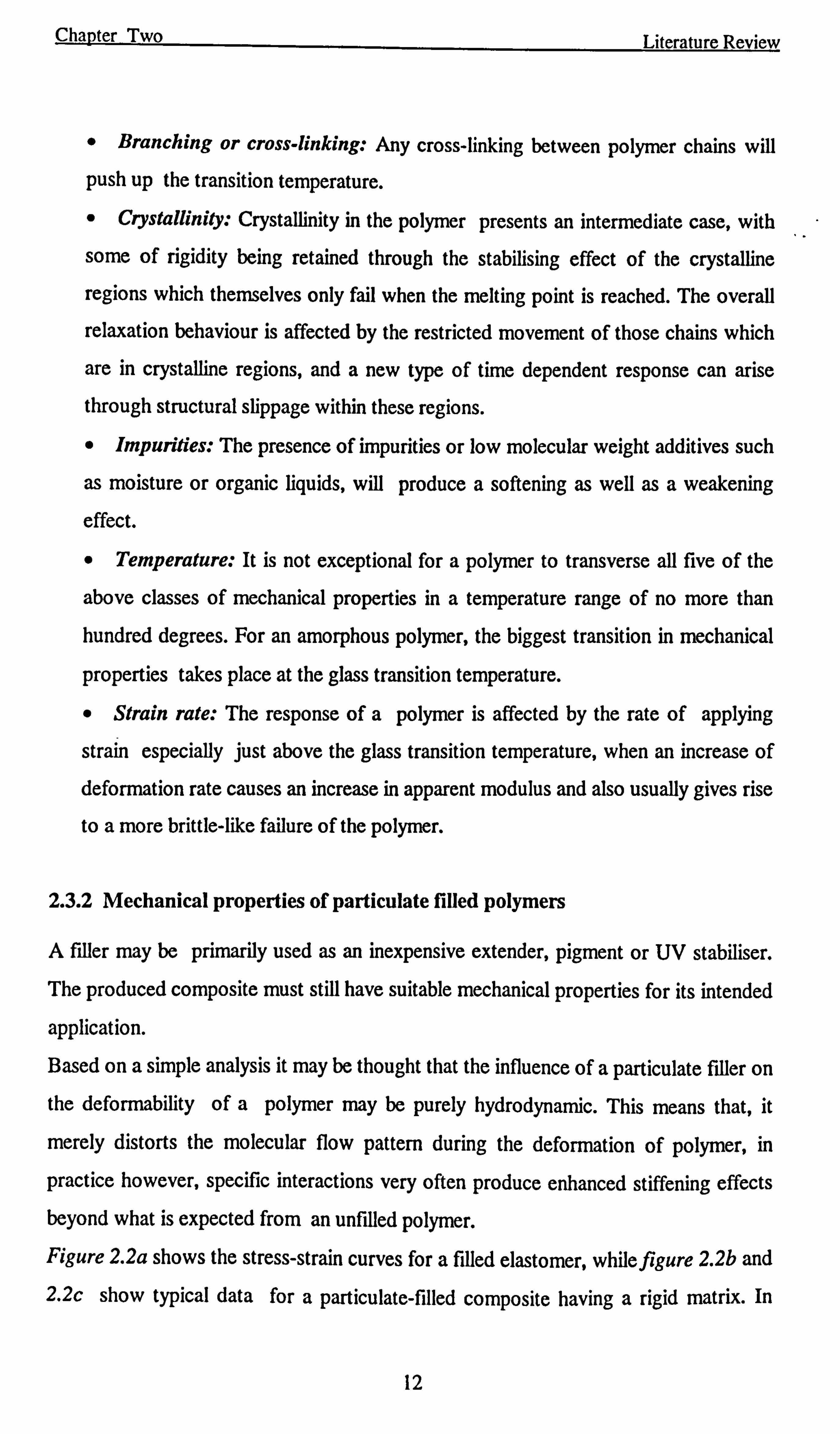
Based on a simple analysis it may be thought that the influence of a particulate filler on
the deformability of a polymer may be purely hydrodynamic. This means that, it
merely distorts the molecular flow pattern during the deformation of polymer, in
practice however, specific interactions very often produce enhanced stiffening effects beyond what is expected from an unfilled polymer. Figure 2.2a shows the stress-strain curves for a filled elastomer, while figure 2.2b and 2.2c show typical data for a particulate-filled composite having a rigid matrix. In
12
Chapter Two Literature Review
both cases, as expected, the modulus increases with increased filler concentration. This
may not always be the case, since if fabrication is accompanied by extensive void formation then the modulus of the produced composite may decrease. It can be seen in
figures 2.2a-2c that the modulus increases for both soft and rigid matrices, while the
tensile strength and elongation at break do not follow the same relationship. The
tensile strength, however, particularly for a rigid matrix with rigid filler decreases with
the increase of filler concentration. This is attributed to an increased concentration
effect as well as the formation of microcracks either at the interface or locally in the
matrix. In the case of a soft elastomeric-based composite, which is capable of
dispersing stress more effectively, the tensile strength may very well increase as a
result of higher filler concentrations. A maximum will be reached in this latter case, if
STRAIN
(01
N
O O
CONCENTRATION (c)
STRAIN
(bI
Fig. 2.2 Stress-strain behaviour of polymer-particulate filler composites
(a) soft matrix, hard filler; (b) hard matrix, soft filler; (c) hard matrix, hard filler
13
Chanter Two Literature Review
for no other reason than that eventually the matrix continuity will be replaced by
particle/particle contact. Thus mechanical coherence except for some agglomeration
will be greatly reduced. On the latter point, it follows that improved dispersion can
have an opposite effect on strength compared to modulus. Considering the other
extreme property, i. e. elongation at break, it might be expected that this quantity will
fall with increasing filler concentration. This is because proportionally, more strain is
being applied to less polymer. However the use of soft fillers in a rigid matrix can
give rise to an increase in elongation at break and also in impact strength. Part of this
may be derived from the ability of some fillers to promote craze formation in deformed
polymer prior to fracture.
Debonding and crack formation generally lower the strength of composites. In certain
cases however, where cross-linked low energy brittle plastics such as polyesters and
epoxides are involved, the actual fracture energy which is distinct from strength, may
be increased by the presence of filler. The fracture energy increases up to quite high
concentrations of filler after which it decreases again.
2.3.3 Non-linear behaviour of polymeric composites
It is usually assumed that composites have a linear mechanical behaviour to avoid the
complexities involved in non-linear analysis. This can hardly be observed even for a
pure polymer. The non-linear behaviour of a material is normally due to the following
factors:
" Non linearity due to material behaviour: Although the first approximation of
constitutive behaviour is usually based on a linear relationship between stress and
strain, many common engineering thermoplastics exhibit a very non-linear stress-
strain relationship. In order to define a non-linear stress-strain relationship, a finite
set of stress-strain data generally provided by experiment, is considered. A
mathematical software is then used to interpolate all other stress-strain values that
are required during a broad analysis.
" Non linearity due to large displacements: A customary assumption in most
engineering analysis is that the displacements are small. The elastic moduli of
polymers are, however, usually as much as two orders of magnitude less than
14
Chapter Two Literature Review
those of materials with simpler behaviour such as metals. Furthermore, plastics will
undergo as much as an order of magnitude more strain before incurring damage.
These phenomena can often result in larger rotations and displacements in plastic
structures than in metals.
" Non linearity due to the load-deformation interaction: A third type of non-
linear behaviour is the result of the interaction of deformation with the application
of load. Linear analysis assumes that the location and distribution of a load in a
system do not change during its deformation. This assumption is not always valid,
especially when deformations become large.
2.4 THEORETICAL MODELS FOR DETERMINATION OF THE
MODULUS OF COMPOSITES
The micromechanical analysis of the mechanical behaviour in terms of the separate
contributions of the two components(i. e. the polymeric matrix and inclusion) to
mechanical properties is complicated. This complication arises not only from
recognised complexities of the filler concentration, but also from uncertainties in the
magnitude of interaction. Especially as the magnitude of interaction might itself vary
as the polymer and filler are mechanically forced into greater contact during
deformation. In addition there are uncertainties in filler size distribution, complicated
by possible agglomeration, and the extent of void formation occurred during
fabrication, and the related problem of imperfect interfacial contact between the
matrix and filler. Nevertheless, theories which describe the mechanical properties of
particulate filled polymers have been developed. Often one theory gives better account
of one situation than other. Modulus of composites is a bulk property which depends
primarily on the geometry, modulus, particle size distribution, and concentration of the
filler and has been represented by a large number of theoretically derived equations.
15
Chapter Two
2.4.1 Theories of rigid inclusions in a non-rigid matrix
2.4.1.1 Einstein equation and its modifications
Literature Review
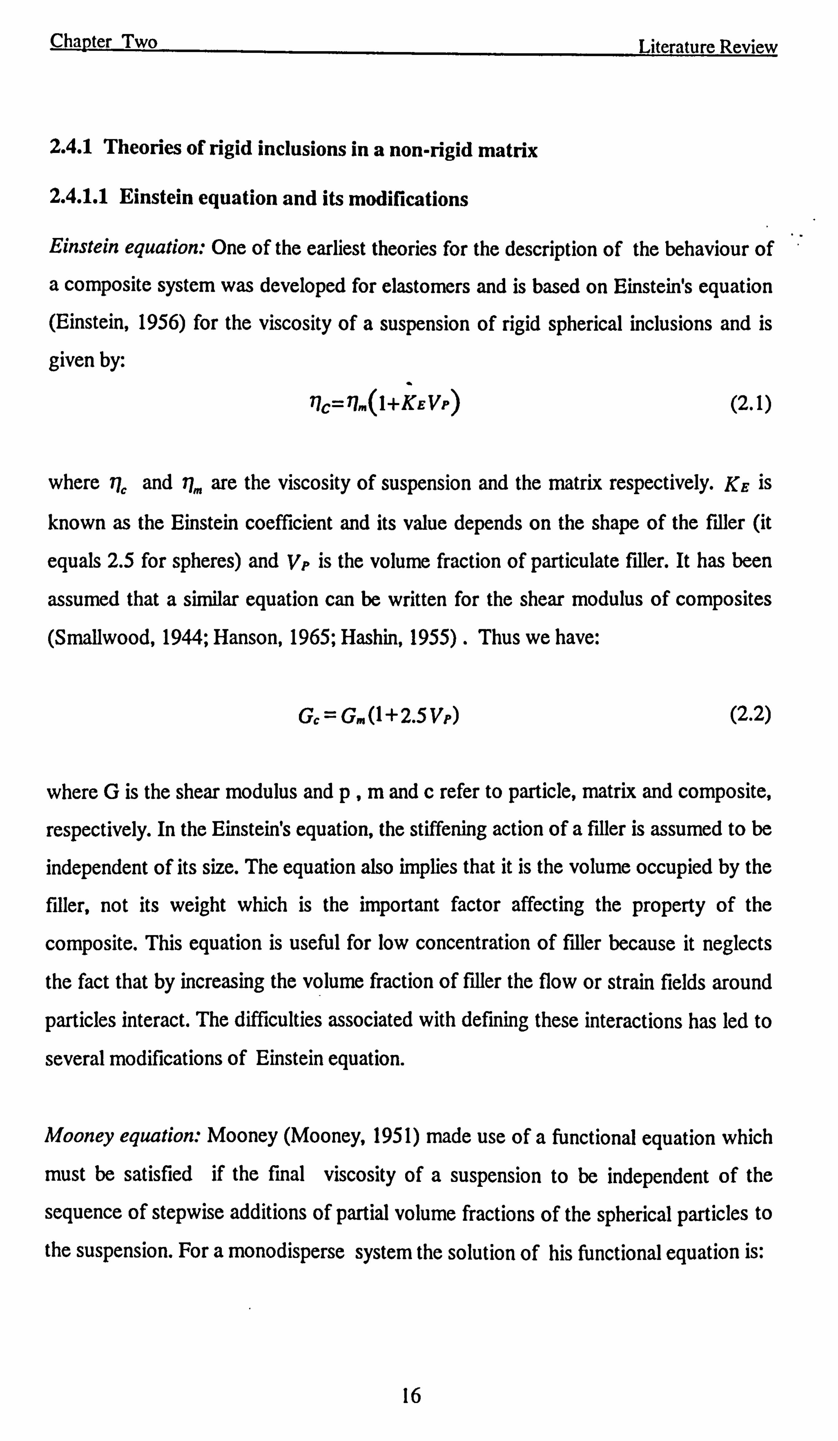
Einstein equation: One of the earliest theories for the description of the behaviour of
a composite system was developed for elastomers and is based on Einstein's equation (Einstein, 1956) for the viscosity of a suspension of rigid spherical inclusions and is
given by:
"IC=llm(I+KEVP) (2.1)
where 17, and r). are the viscosity of suspension and the matrix respectively. KE is
known as the Einstein coefficient and its value depends on the shape of the filler (it
equals 2.5 for spheres) and VP is the volume fraction of particulate filler. It has been
assumed that a similar equation can be written for the shear modulus of composites
(Smallwood, 1944; Hanson, 1965; Hashin, 1955). Thus we have:
G, =Gm(1+2.5vP) (2.2)
where G is the shear modulus and p, m and c refer to particle, matrix and composite,
respectively. In the Einstein's equation, the stiffening action of a filler is assumed to be
independent of its size. The equation also implies that it is the volume occupied by the
filler, not its weight which is the important factor affecting the property of the
composite. This equation is useful for low concentration of filler because it neglects
the fact that by increasing the volume fraction of filler the flow or strain fields around
particles interact. The difficulties associated with defining these interactions has led to
several modifications of Einstein equation.
Mooney equation: Mooney (Mooney, 1951) made use of a functional equation which
must be satisfied if the final viscosity of a suspension to be independent of the
sequence of stepwise additions of partial volume fractions of the spherical particles to
the suspension. For a monodisperse system the solution of his functional equation is:
16
Chanter Two Literature Review
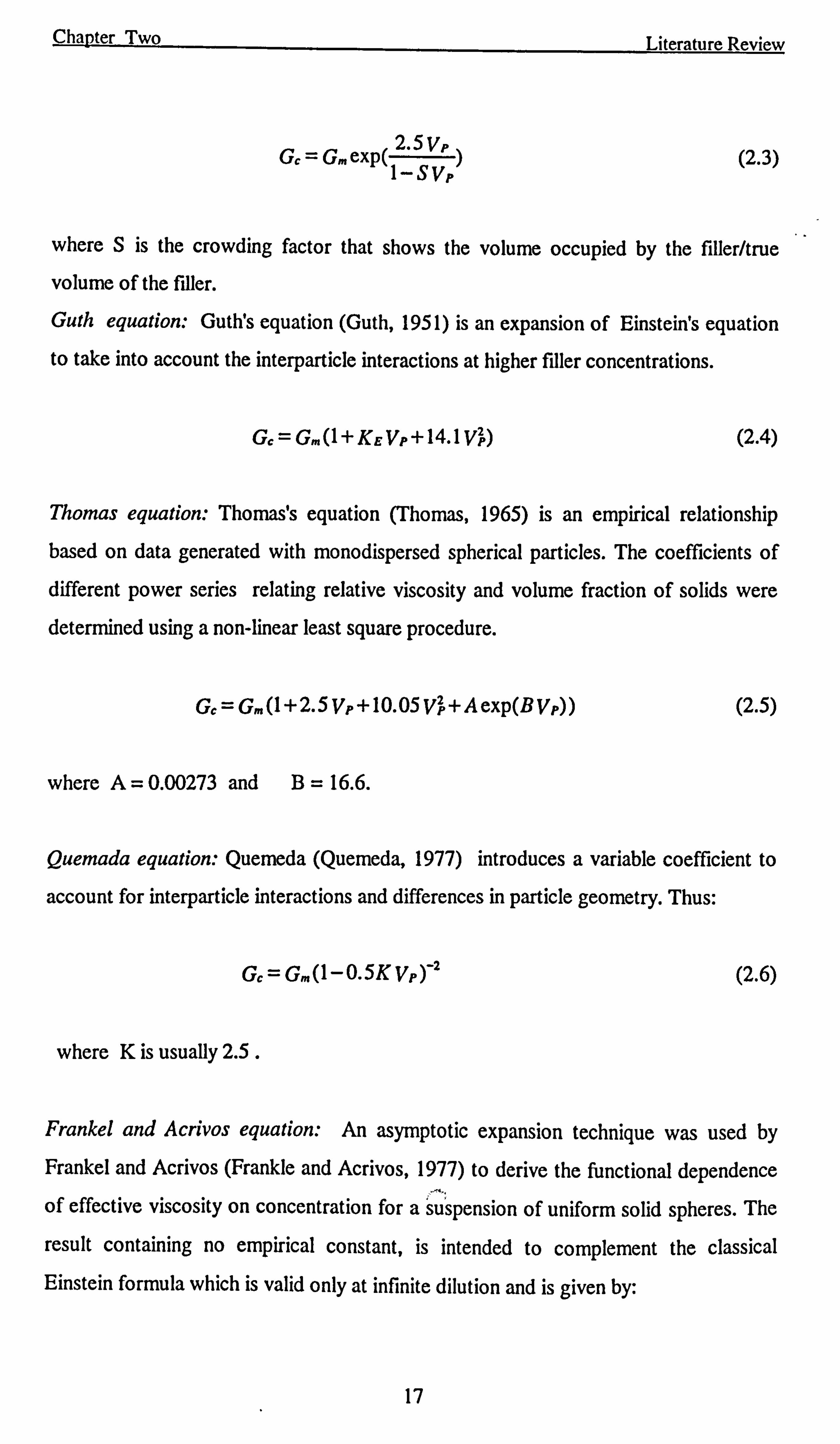
Gc=GmeXp( 2.5 VP ý
1-SVP (2.3)
where S is the crowding factor that shows the volume occupied by the filler/true
volume of the filler.
Guth equation: Guth's equation (Guth, 1951) is an expansion of Einstein's equation to take into account the interparticle interactions at higher filler concentrations.
G2) VP) (2.4)
Thomas equation: Thomas's equation (Thomas, 1965) is an empirical relationship based on data generated with monodispersed spherical particles. The coefficients of different power series relating relative viscosity and volume fraction of solids were determined using a non-linear least square procedure.
Gc=G, �(1+2.5Vp+10.05Vp+Aexp(BVp)) (2.5)
where A= 0.00273 and B= 16.6.
Quemada equation: Quemeda (Quemeda, 1977) introduces a variable coefficient to
account for interparticle interactions and differences in particle geometry. Thus:
G, =G,. (1-0.5K VP )-2 (2.6)
where K is usually 2.5.
Frankel and Acrivos equation: An asymptotic expansion technique was used by
Frankel and Acrivos (Frankle and Acrivos, 1977) to derive the functional dependence
of effective viscosity on concentration for a suspension of uniform solid spheres. The
result containing no empirical constant, is intended to complement the classical Einstein formula which is valid only at infinite dilution and is given by:
17
Chapter Two
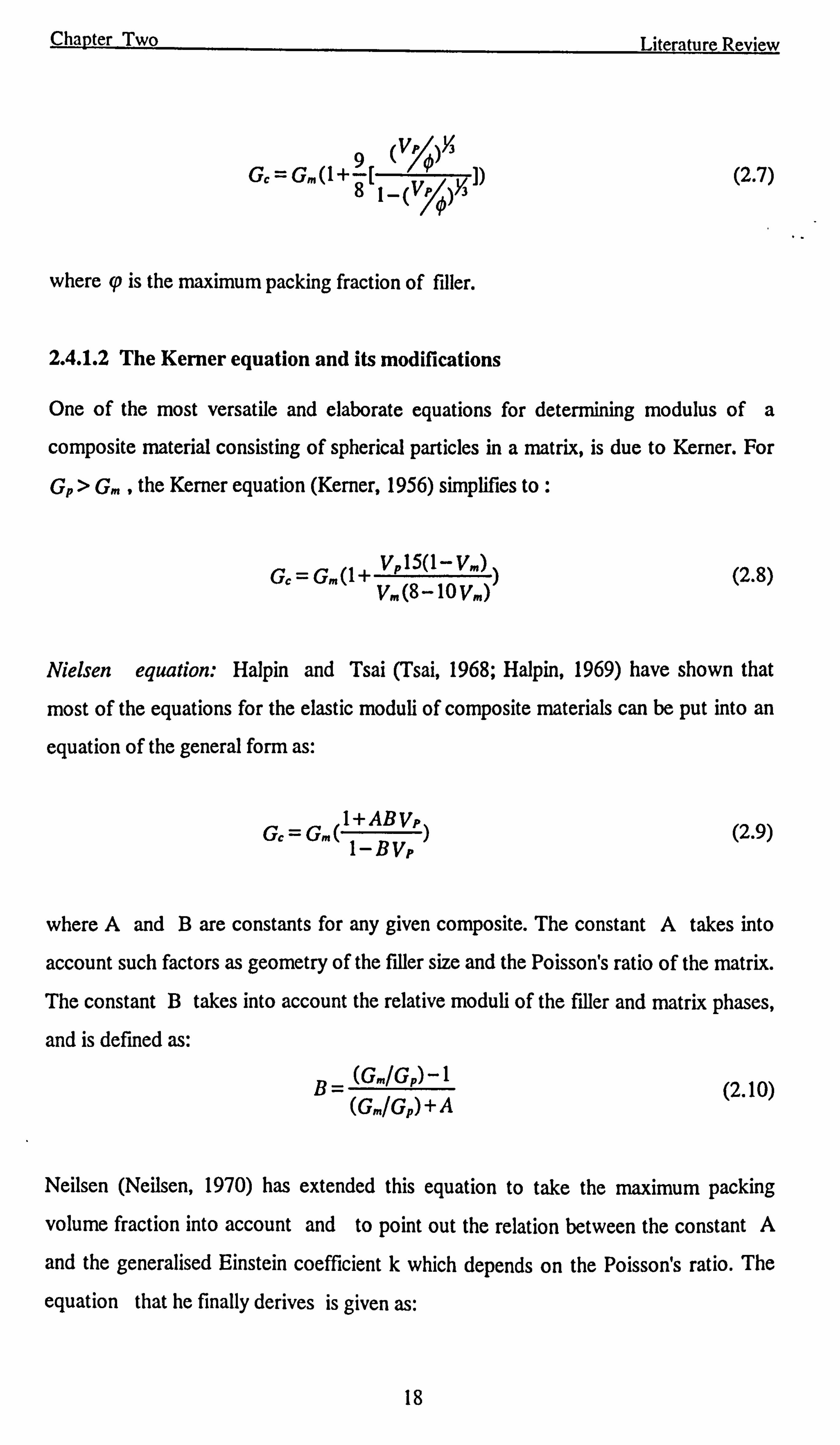
^^ /t (`'/) y l7c =llmll+9o 1ý-(i,
/)V ýý
where (P is the maximum packing fraction of filler.
2.4.1.2 The Kerner equation and its modifications
Literature Review
(2.7)
One of the most versatile and elaborate equations for determining modulus of a
composite material consisting of spherical particles in a matrix, is due to Kerner. For
Gp > G. , the Kerner equation (Kerner, 1956) simplifies to :
11t=`jmýl ý VPl5(l-ym)`
vm(8-lOvm) (2.8)
Nielsen equation: Halpin and Tsai (Tsai, 1968; Halpin, 1969) have shown that
most of the equations for the elastic moduli of composite materials can be put into an
equation of the general form as:
G=Gm(1+ABVpý 1-BVP
(2.9)
where A and B are constants for any given composite. The constant A takes into
account such factors as geometry of the filler size and the Poisson's ratio of the matrix.
The constant B takes into account the relative moduli of the filler and matrix phases,
and is defined as:
B_ (GmlGp) -I
(GmlGp) +A (2.10)
Neilsen (Neilsen, 1970) has extended this equation to take the maximum packing
volume fraction into account and to point out the relation between the constant A
and the generalised Einstein coefficient k which depends on the Poisson's ratio. The
equation that he finally derives is given as:
18
Chapter Two
Gc =Gm(1+(k-1)BVP) 1-BVP
2.4.2 Theories of non-rigid inclusions in a non-rigid matrix
(2.11)
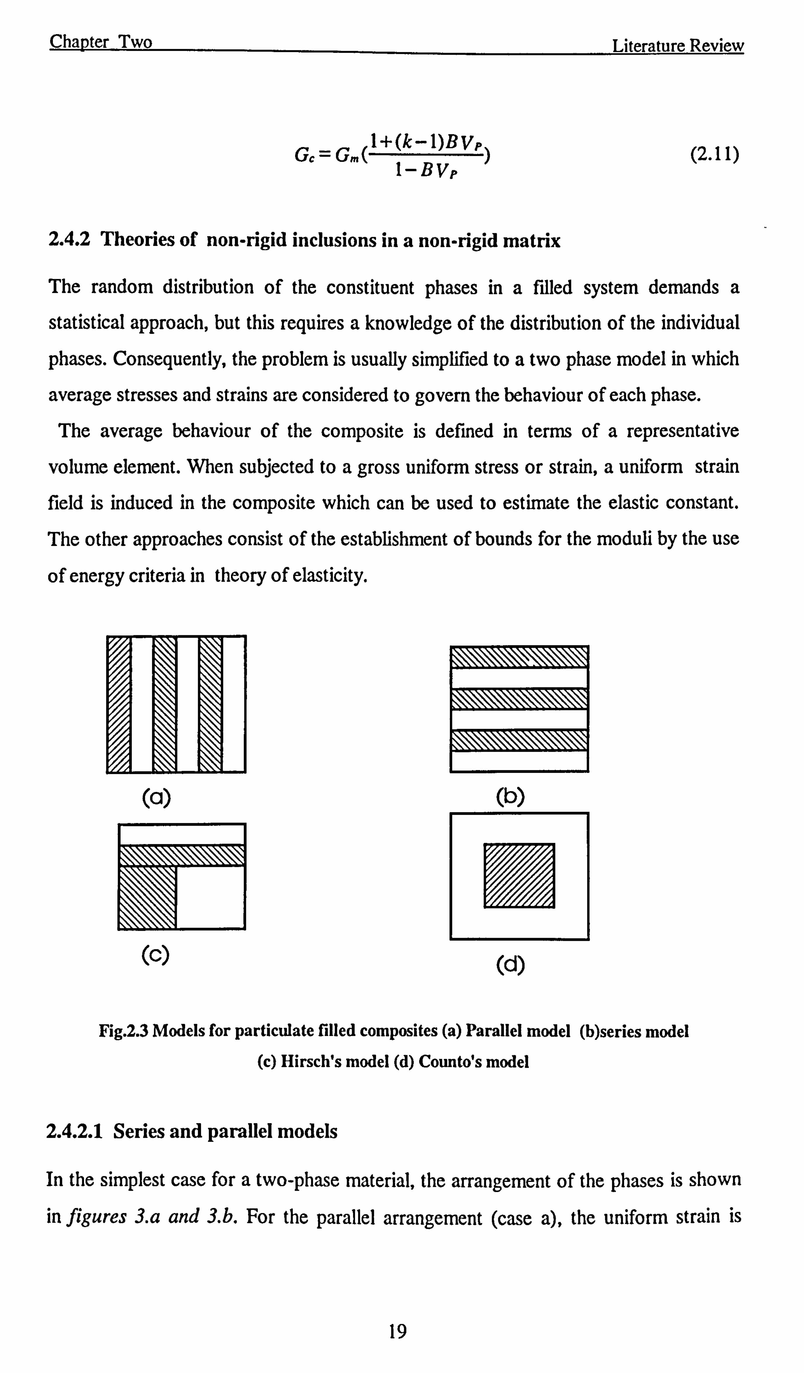
The random distribution of the constituent phases in a filled system demands a
statistical approach, but this requires a knowledge of the distribution of the individual
phases. Consequently, the problem is usually simplified to a two phase model in which
average stresses and strains are considered to govern the behaviour of each phase.
The average behaviour of the composite is defined in terms of a representative
volume element. When subjected to a gross uniform stress or strain, a uniform strain
field is induced in the composite which can be used to estimate the elastic constant.
The other approaches consist of the establishment of bounds for the moduli by the use
of energy criteria in theory of elasticity.
(a)
(c) (a)
Fig. 2.3 Models for particulate filled composites (a) Parallel model (b)series model (c) Hirsch's model (d) Counto's model
2.4.2.1 Series and parallel models
In the simplest case for a two-phase material, the arrangement of the phases is shown
in figures 3. a and 3. b. For the parallel arrangement (case a), the uniform strain is
(b)
Literature Review
19
Chapter Two Literature Review
assumed in the two phase and the upper bound is given by (Broutman and Krock,
1967):
Gc= Gm Vm + GP VP ý2.12ý
whereas in series arrangement (case b) the stress assumed to be uniform in the two
phases. The lower bound is
GP Gm G,
GPVm+G. VP (2.13)
In equation 2.12 it is assumed that the Poisson's ratios of constituent phases are equal.
Whereas using equation 2.13 vv , the corresponding Poisson's ratio should be given
by:
(vpVPGm+ umVmGp)
(VpGm+Vm Gp) (2.14)
The upper and lower bounds obtained from equations 2.12 and 2.13 often do not
represent the experimental data. This implies that the assumption of either a state of
uniform strain or uniform stress in the individual phases of the filled system is not
sufficient to describe the modulus.
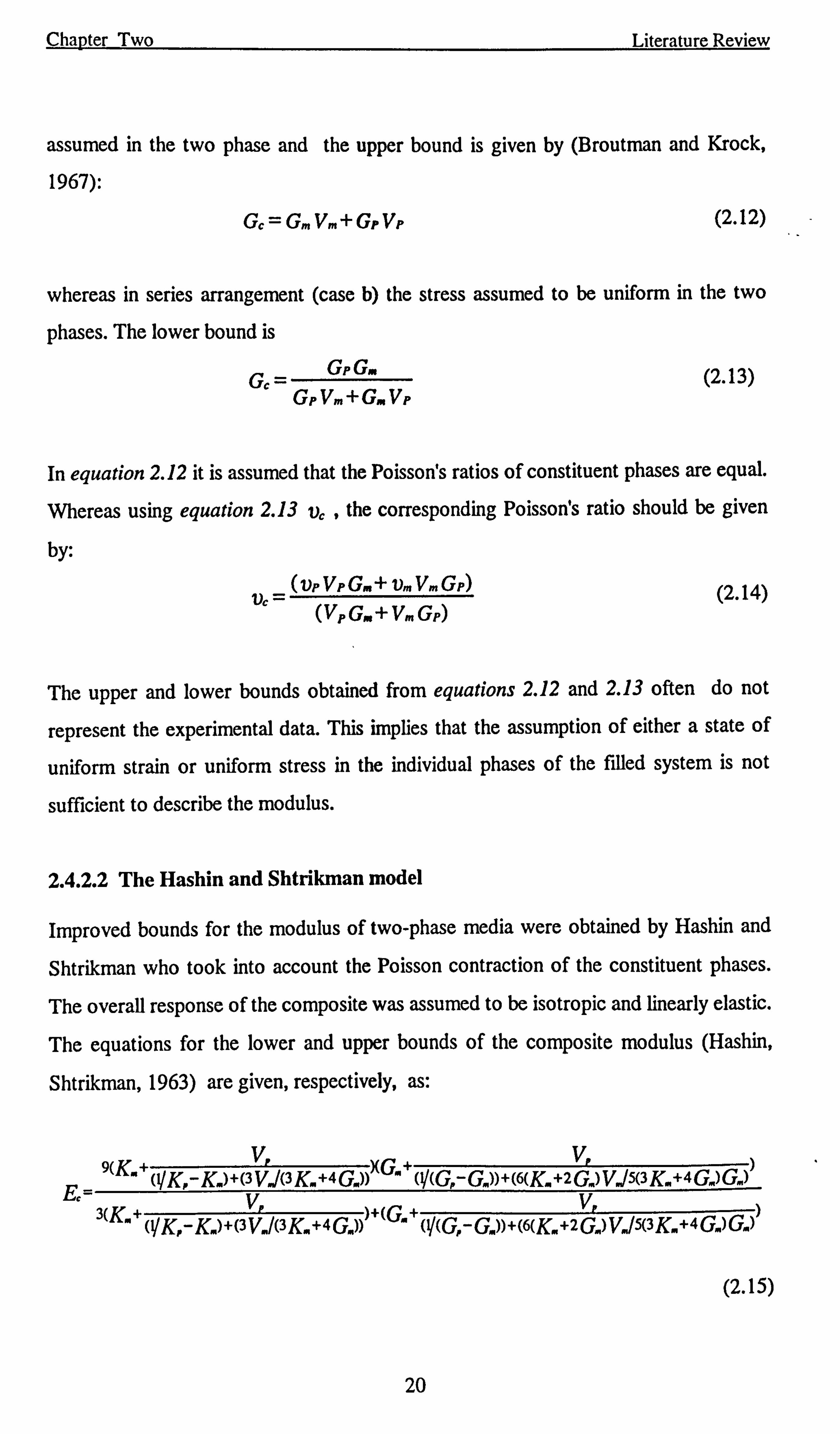
2.4.2.2 The Hashin and Shtrikman model
Improved bounds for the modulus of two-phase media were obtained by Hashin and
Shtrikman who took into account the Poisson contraction of the constituent phases.
The overall response of the composite was assumed to be isotropic and linearly elastic.
The equations for the lower and upper bounds of the composite modulus (Hashin,
Shtrikman, 1963) are given, respectively, as:
9(K. +(VKr-K. )+(3V. J(3 K. +4 G. ))xG'+TV(Gr-G. ))+(6(K. +2G. )VJS(3 K., +4G. )G. )) V, VP E, -3(K,
+(VK, - Y K. )+(3V. 1(3K. +4G., )))+(G. +((Gr
-G. ))+(6(K. +2G. )V. 15(3K. +4Gý)G. ))
(2.15)
20
Chapter Two Literature Review
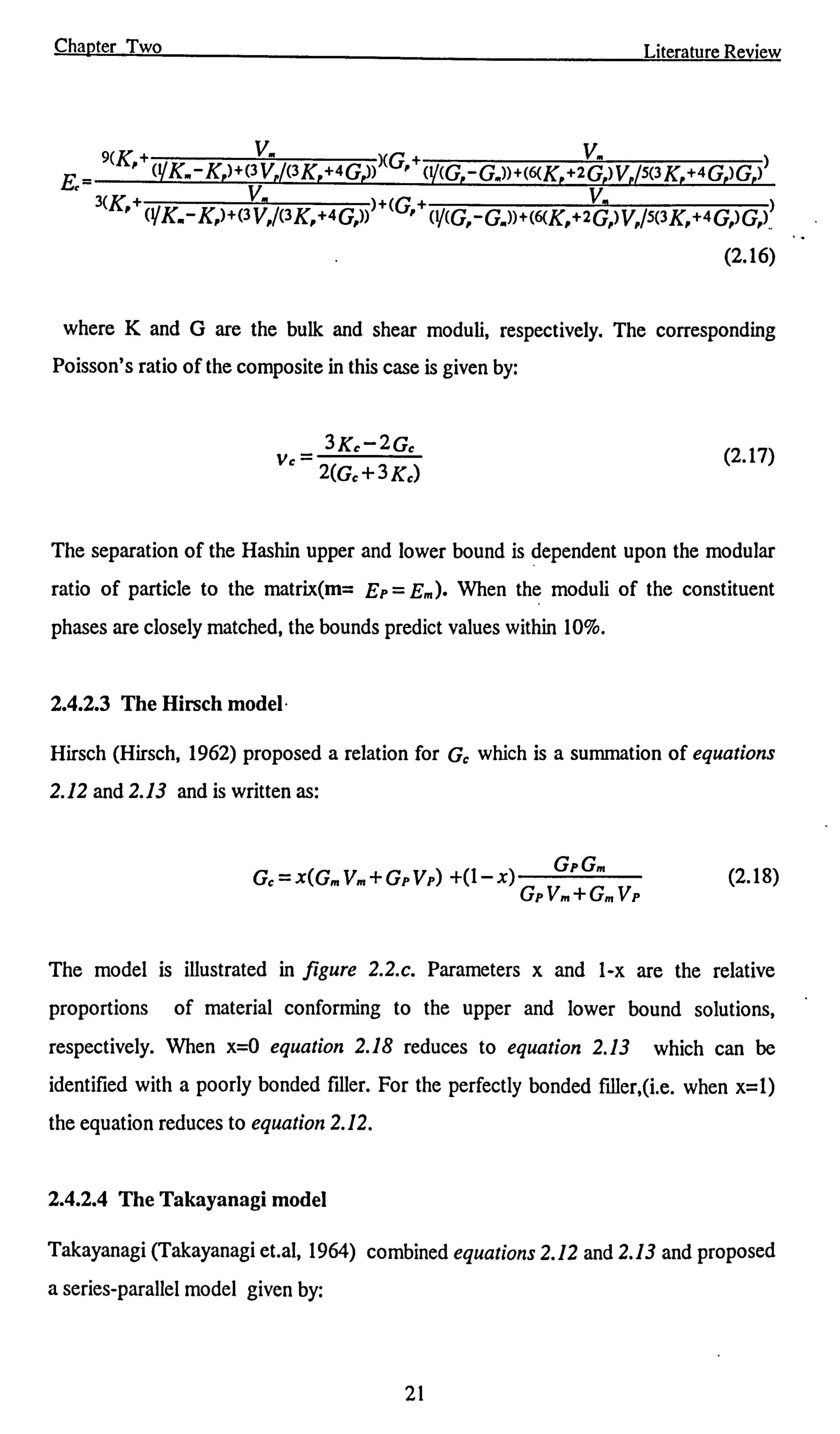
+ V. + V. 9(K' (yK., -K, )+(3V, /(3K, +4G, )))(G, (i/(G, -G. ))+(6(j{, +2G, )VP/s(3K, +4G, )G, ))
3(K,, + V. V)
cyK. -K, )+(3V . l(3K. +4G, )))+(G, + (V(G, - G, )) +cýK, +2 G, )V, /s(3K. +4 G, ) G,, )., (2.16)
where K and G are the bulk and shear moduli, respectively. The corresponding Poisson's ratio of the composite in this case is given by:
V. - = 3K, -2G, (2.17)
- 2(G, +3K, )
The separation of the Hashin upper and lower bound is dependent upon the modular
ratio of particle to the matrix(m= EP = E. ). When the moduli of the constituent
phases are closely matched, the bounds predict values within 10%.
2.4.2.3 The Hirsch model,
Hirsch (Hirsch, 1962) proposed a relation for G, which is a summation of equations
2.12 and 2.13 and is written as:
Gt=X(GmVm+GPVP) +(1-X) GPGm
GPVm+GmVP (2.18)
The model is illustrated in figure 2.2. c. Parameters x and 1-x are the relative
proportions of material conforming to the upper and lower bound solutions,
respectively. When x=0 equation 2.18 reduces to equation 2.13 which can be
identified with a poorly bonded filler. For the perfectly bonded filler, (i. e. when x=1)
the equation reduces to equation 2.12.
2.4.2.4 The Takayanagi model
Takayanagi (Takayanagi et. al, 1964) combined equations 2.12 and 2.13 and proposed
a series-parallel model given by:
21
Chanter Two Literature Review
Gc =(a+ (1- a) )-ý (1- P'Gm+ßGP GP
(2.19)
where parameters a and ß represent the state of parallel and series coupling in the
composite, respectively. Equation 2.19 was developed to predict the modulus of a
crystalline polymer. The basic problem with this model is the determination of values
for a and P. The arrangement of the series and parallel element is, however, an
inherent difficulty in all of the proceeding models and there are conceptual difficulties
in relating these models to real systems.
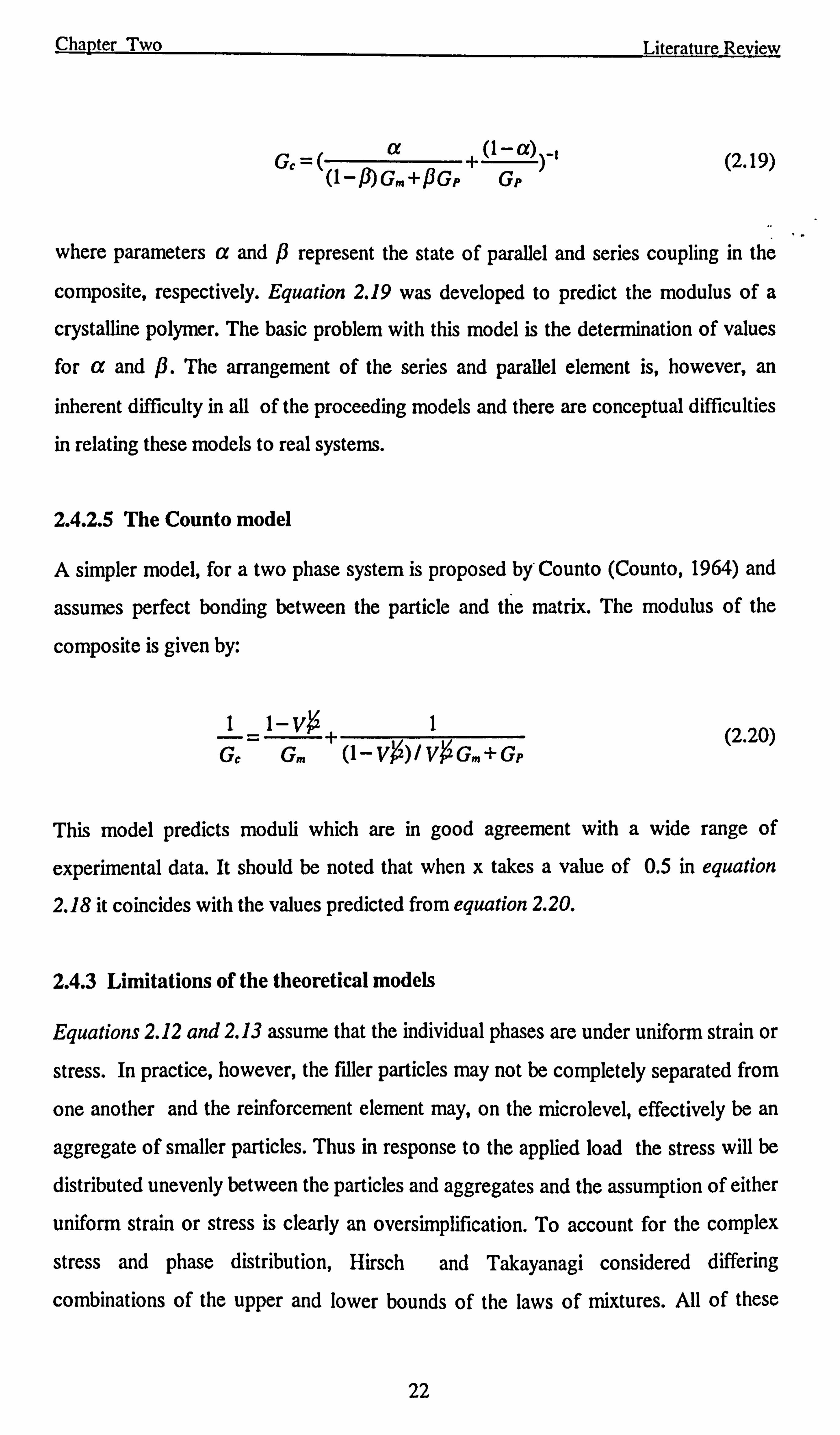
2.4.2.5 The Counto model
A simpler model, for a two phase system is proposed by Counto (Counto, 1964) and
assumes perfect bonding between the particle and the matrix. The modulus of the
composite is given by:
i _1-vý+ 1 G, G, � (1-Vg)I VgG, �+Gr
(2.20)
This model predicts moduli which are in good agreement with a wide range of
experimental data. It should be noted that when x takes a value of 0.5 in equation
2.18 it coincides with the values predicted from equation 2.20.
2.4.3 Limitations of the theoretical models
Equations 2.12 and 2.13 assume that the individual phases are under uniform strain or
stress. In practice, however, the filler particles may not be completely separated from
one another and the reinforcement element may, on the microlevel, effectively be an
aggregate of smaller particles. Thus in response to the applied load the stress will be
distributed unevenly between the particles and aggregates and the assumption of either
uniform strain or stress is clearly an oversimplification. To account for the complex
stress and phase distribution, Hirsch and Takayanagi considered differing
combinations of the upper and lower bounds of the laws of mixtures. All of these
22
Chapter Two Literature Review
require an empirical factor which is determined by a curve fitting routine to furnish a
phenomenological description of the experimental data.
Theories which deal with filled systems indicate that the elastic modulus for a given
particle and matrix depends only upon the volume fraction of filler and not the particle
size. The modulus however, increases as the particle size decreases.
The properties of the composites may also be affected by changes in particle shape.
This effect is especially pronounced with larger or non-spherical particles where a
preferred orientation can modify the particle deformation behaviour.
The particle size distribution affects the maximum packing fraction 0'.. Mixtures of
particles with differing sizes can pack more densely than monodispersed particles
because the small ones can fill the space between the closely packed large particles to
form an agglomerate. These aggregated particles may be able to carry a large
proportion of the load than the primary particles to yield a higher modulus, at the same
volume fraction.
Most of the theories which explain the reinforcing action of a filler assume perfect
adhesion between the filler and the polymer matrix. The case of imperfect adhesion
was, however, discussed theoretically by Sato and Furukawa (Sato and Furukawa,
1963). They assumed that the non-bonded particles act as holes and, therefore,
predicted a decrease in modulus with increasing filler content. One can argue that the
non-bonded particles do not act entirely as holes since they also restrain the matrix
from collapsing. A change of the matrix-filler adhesion has a smaller effect on modulus
than on strength. The latter is much more dependent on surface pretreatment. In fact,
the degree of adhesion does not appear to be an important factor as long as the
frictional forces between the phases are not exceeded by the applied stress. In most
filled systems there is a mismatch in the coefficients of thermal expansion which is
reflected as a mechanical bond resulting from thermally induced stresses. Brassell
(Brassell and Wischmann, 1974) found that the degree of bonding between the phases
does not appear to have any influence on mechanical properties at liquid nitrogen
temperature and this was attributed to the compressive stresses on the filler particle. In
most cases even if the adhesion between phases is poor the theories remain valid as
23
Chapter Two Literature Review
long as there is not a relative motion across the filler-matrix interface(no slip case)
(Ahmed and Jones, 1990).
2.5 MICROMECHANICAL ANALYSIS OF POLYMERIC COMPOSITES
It would be an impossible task to analyse composite materials behaviour by keeping
track of the strains, strain rates and strain gradients within and around each and every
inclusion in the material. At the other end of the scale, we could simply assume that
the individual phases do not exist, measure the macroscopic properties and proceed
with the structural design task(macromechanical analysis). This approach, while
practical, ignores the main opportunity and challenge of composite materials, namely
to tailor the microscale features and characteristics to achieve desired and optimal
macroscopic behaviour. Thus we are naturally led to the problem of averaging the
microscale effects and characteristics to predict the macroscopic behaviour and to
investigate the effects of microstructure, particle size, particle distribution and
interface on the final properties (micromechanical analysis).
The microscale geometry of composite materials involves both deterministic and
statistical features. In proceeding with micromechanical analysis, a cell size is selected
and averaging is done on this scale. The scales for different methods are
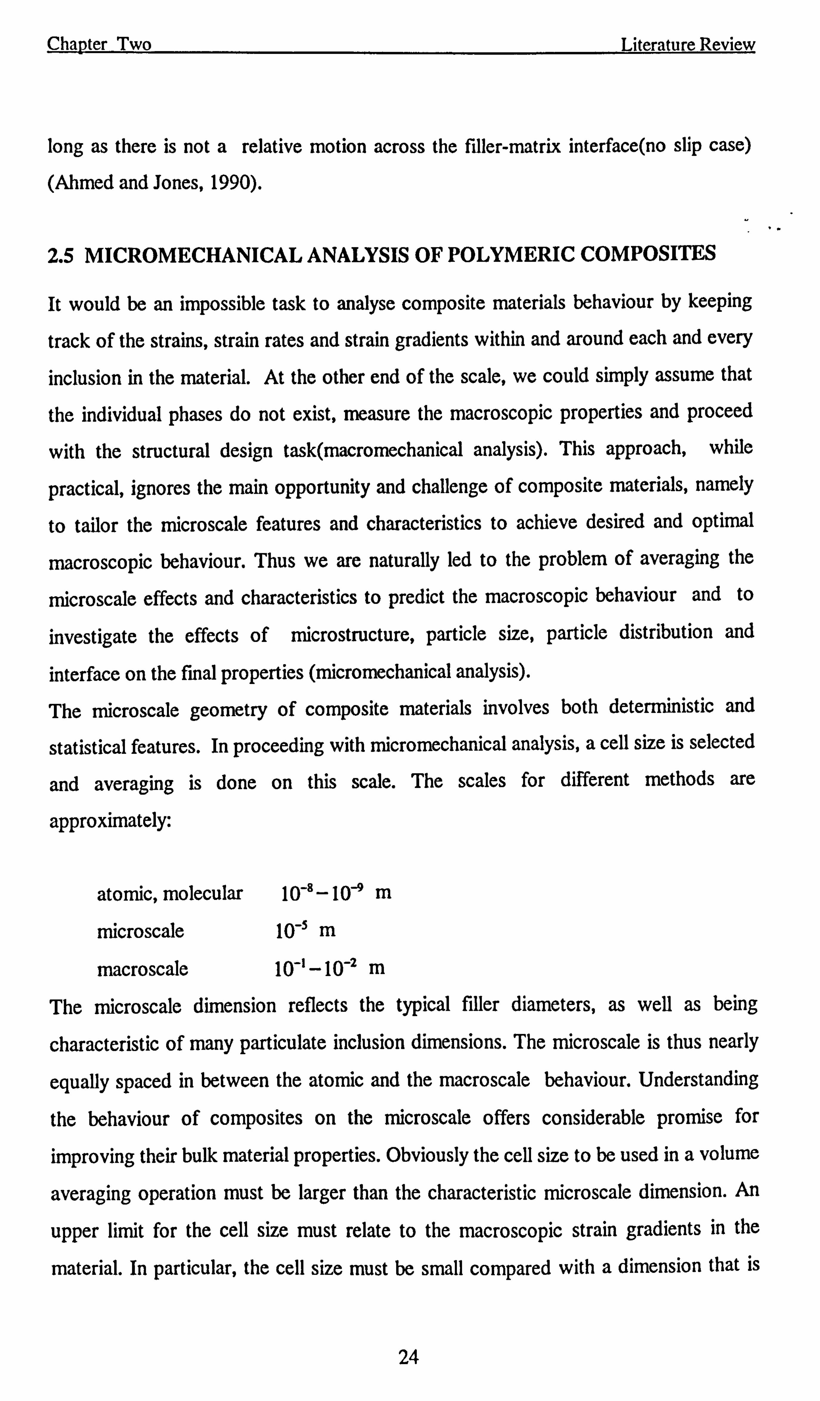
approximately:
atomic, molecular 10-8 -10-9 m
microscale 10-5 m
macroscale 10-1_10-2 m
The microscale dimension reflects the typical filler diameters, as well as being
characteristic of many particulate inclusion dimensions. The microscale is thus nearly
equally spaced in between the atomic and the macroscale behaviour. Understanding
the behaviour of composites on the microscale offers considerable promise for
improving their bulk material properties. Obviously the cell size to be used in a volume
averaging operation must be larger than the characteristic microscale dimension. An
upper limit for the cell size must relate to the macroscopic strain gradients in the
material. In particular, the cell size must be small compared with a dimension that is
24
Chapter Two Literature Review
characteristic of the inverse of the strain gradient. Averaging is done with regard to
cell sizes on the scale of the inhomogeneity. Further to statistical averaging certain
features of the composites such as isotropic behaviour of system with no preferred
orientation are usually used to develop microstructural models (Christensen, 1982).
2.5.1 Qualitative description of the microstructure
2.5.1.1 Geometric models
The procedure typically used to determine macroscopic properties involves the
analysis of a representative cell or volume element of the material. Most of the cell
geometries apply equally well to the cases of fibres or particulate inclusions when
viewed in either cylindrical or spherical coordinates. The composite sphere model was
introduced by Hashin and the corresponding composite cylinders models by Hashin
and Rosen (Hashin and Rosen 1964). A gradation of sizes of cells is assumed such that
a volume filling configuration is obtained. A fixed ratio of cylinders' radii is assumed
such that the analysis of single sphere can be taken to be the representative of the
entire composite system.
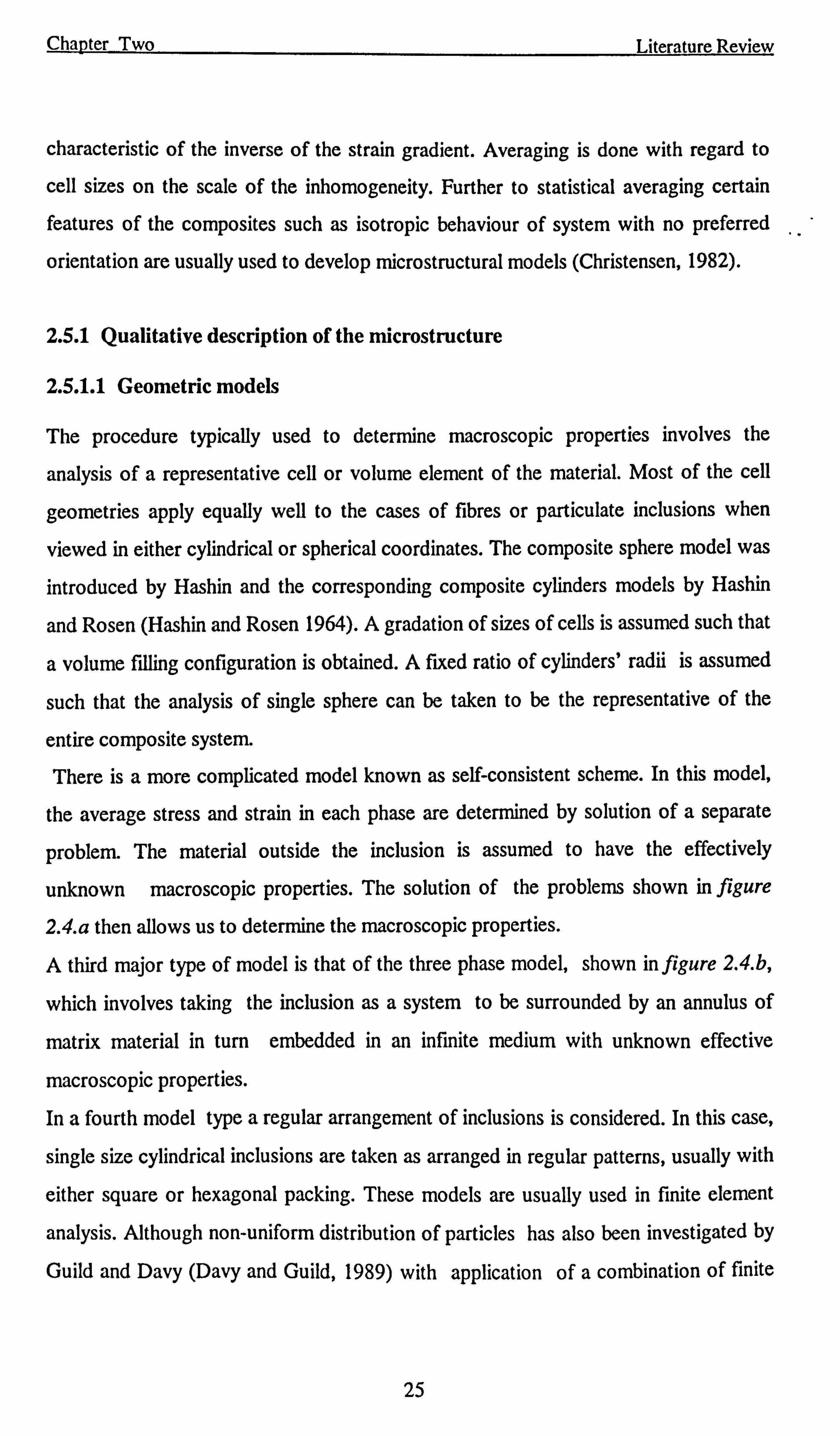
There is a more complicated model known as self-consistent scheme. In this model,
the average stress and strain in each phase are determined by solution of a separate
problem. The material outside the inclusion is assumed to have the effectively
unknown macroscopic properties. The solution of the problems shown in figure
2.4. a then allows us to determine the macroscopic properties.
A third major type of model is that of the three phase model, shown in figure 2.4. b,
which involves taking the inclusion as a system to be surrounded by an annulus of
matrix material in turn embedded in an infinite medium with unknown effective
macroscopic properties.
In a fourth model type a regular arrangement of inclusions is considered. In this case,
single size cylindrical inclusions are taken as arranged in regular patterns, usually with
either square or hexagonal packing. These models are usually used in finite element
analysis. Although non-uniform distribution of particles has also been investigated by
Guild and Davy (Davy and Guild, 1989) with application of a combination of finite
25
Chapter Two Literature Review
element and statistical calculations. The described geometrical models are usually used
to formulate the finite element analysis of stress-strain behaviour of composites.
(a)
phase 1
(b) Fig. 2.4 (a) Self consistent model (b) Three phase model
There is no limit in how many microscopic geometrical models can be designed for
composite behaviour analysis. For example, results applicable to second order in
volume fraction can be obtained by the analysis of just two interacting inclusions in an
infinite medium. At dilute concentrations, ellipsoidal inclusions can be used to
represent a variety of geometric shapes. Also, ellipsoidal inclusions are also directly
related to the self-consistent scheme (Christensen, 1982).
2.5.1.2 Geometric model used in finite element modelling of composites
Although usually a periodic distribution of particles are chosen, there is possibility of
studying nonuniform distribution through using statistical calculations such as the
model due to Guild and Davy. In this model, spherical particles of equal diameter are
assumed to be randomly distributed within an infinite matrix. Finite element analysis is
performed for a cylinder of resin, radius equal half-height, R, containing a single
sphere at its centre, radius r. This cylinder can be represented by the plane ABCD
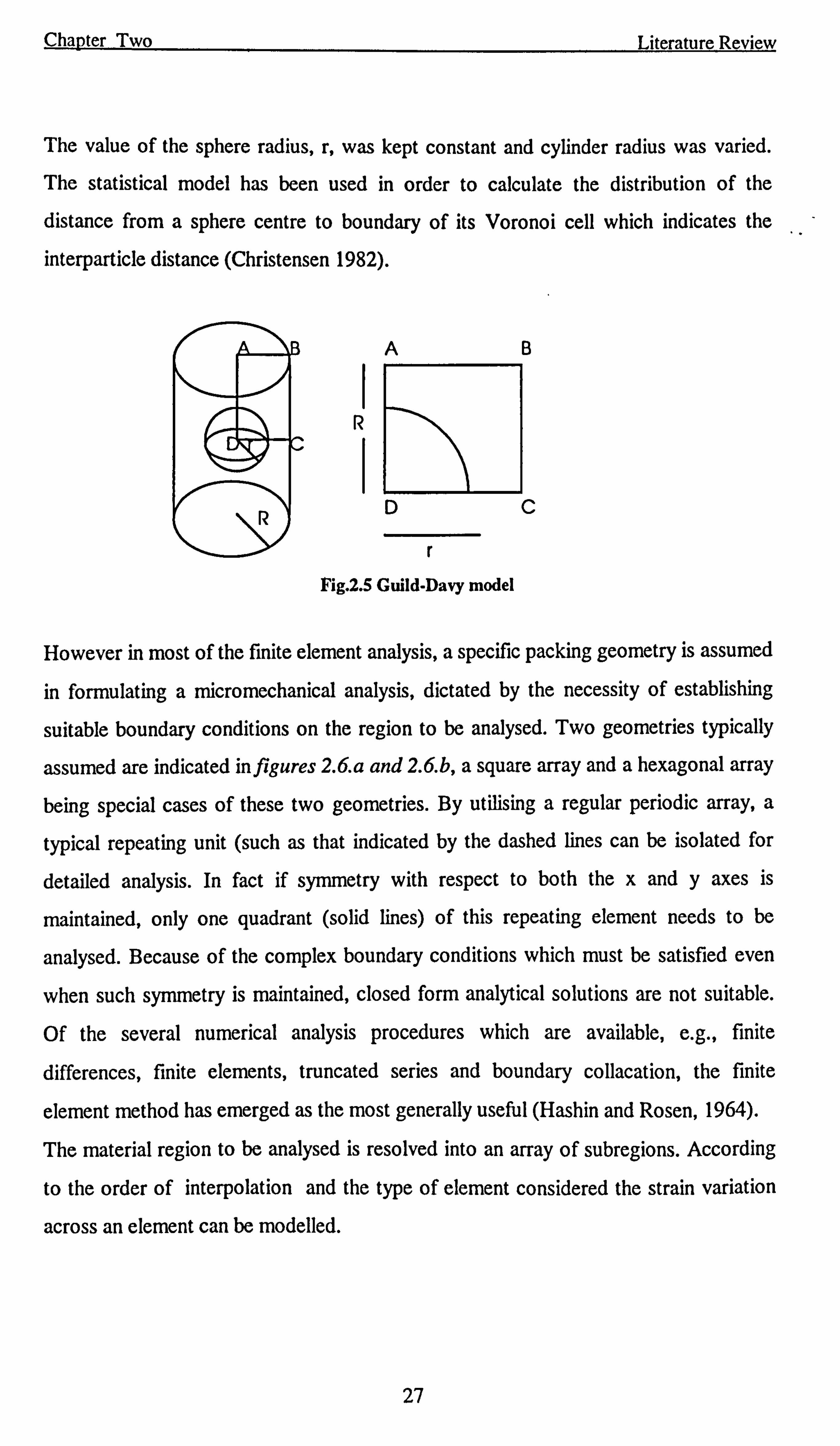
using axisymmetric elements (figure 2.5).
phase 2
26
Chapter Two Literature Review
The value of the sphere radius, r, was kept constant and cylinder radius was varied. The statistical model has been used in order to calculate the distribution of the
distance from a sphere centre to boundary of its Voronoi cell which indicates the
interparticle distance (Christensen 1982).
A
r Fig. 2.5 Guild-Davy model
B
C
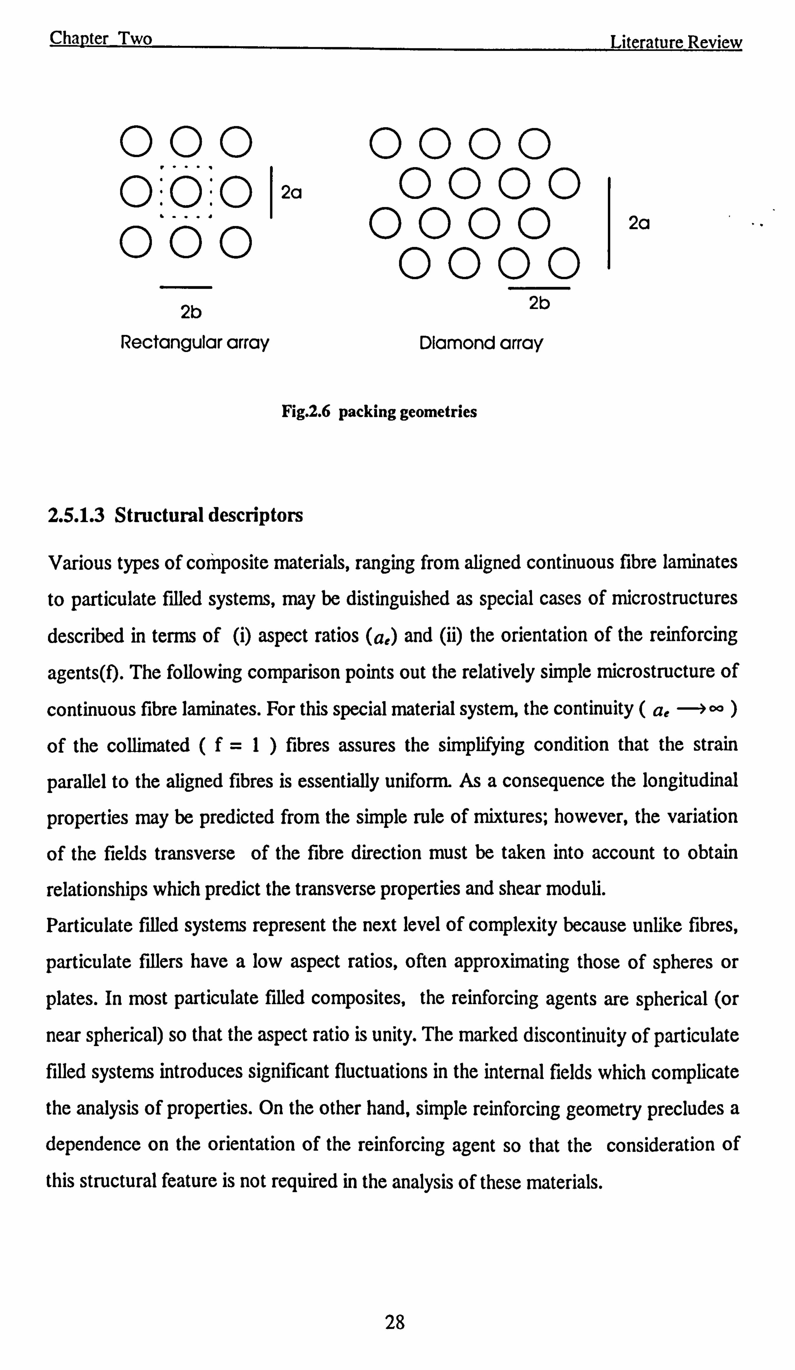
However in most of the finite element analysis, a specific packing geometry is assumed
in formulating a micromechanical analysis, dictated by the necessity of establishing
suitable boundary conditions on the region to be analysed. Two geometries typically
assumed are indicated in figures 2.6. a and 2.6b, a square array and a hexagonal array
being special cases of these two geometries. By utilising a regular periodic array, a
typical repeating unit (such as that indicated by the dashed lines can be isolated for
detailed analysis. In fact if symmetry with respect to both the x and y axes is
maintained, only one quadrant (solid lines) of this repeating element needs to be
analysed. Because of the complex boundary conditions which must be satisfied even
when such symmetry is maintained, closed form analytical solutions are not suitable.
Of the several numerical analysis procedures which are available, e. g., finite
differences, finite elements, truncated series and boundary collacation, the finite
element method has emerged as the most generally useful (Hashin and Rosen, 1964).
The material region to be analysed is resolved into an array of subregions. According
to the order of interpolation and the type of element considered the strain variation
across an element can be modelled.
27
Chapter Two
000 0000 QQQ2a 0000 000 0000
2b 2b
Rectangular array Diamond array
Fig. 2.6 packing geometries
2.5.1.3 Structural descriptors
Literature Review
2a
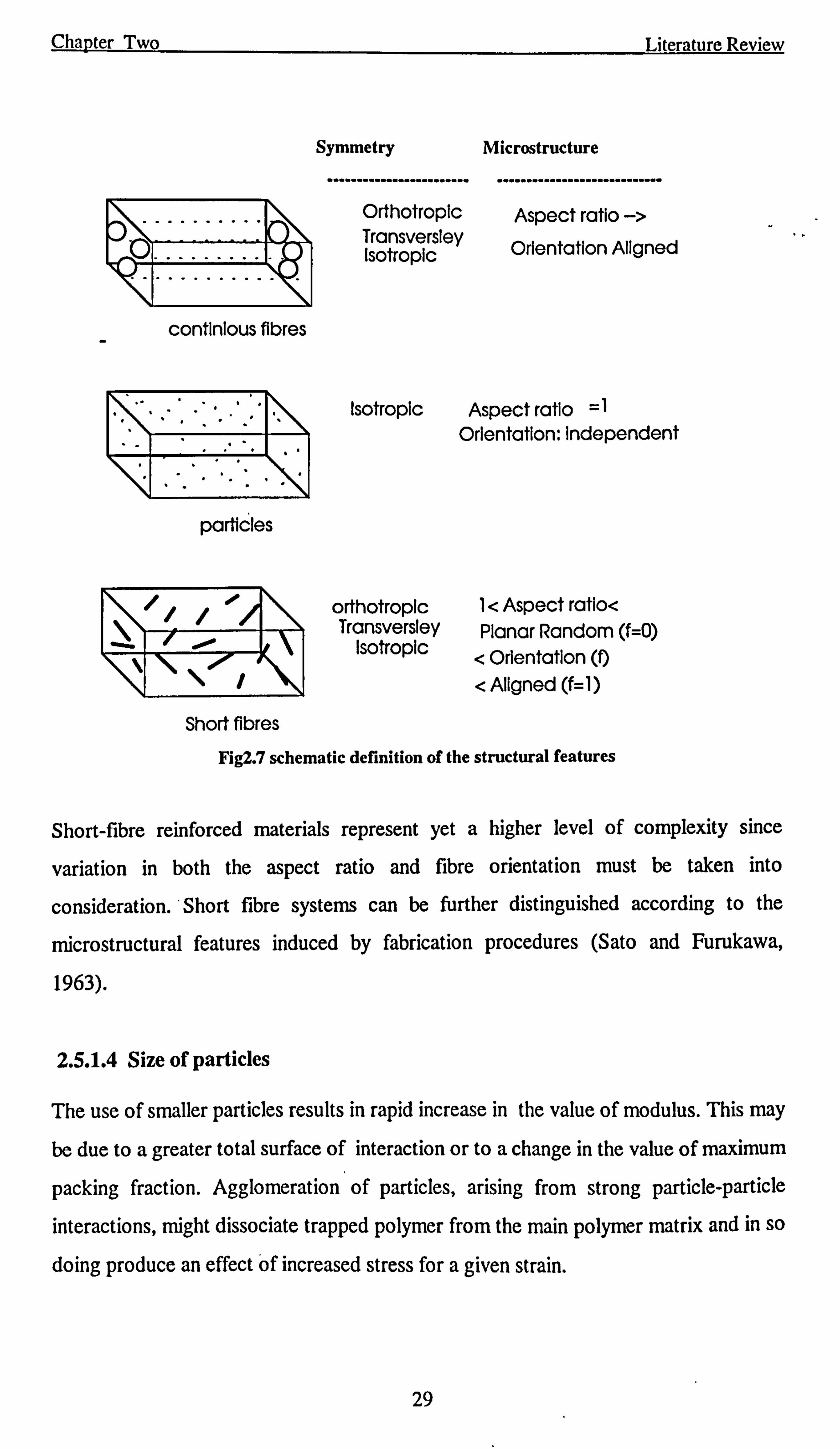
Various types of composite materials, ranging from aligned continuous fibre laminates
to particulate filled systems, may be distinguished as special cases of microstructures
described in terms of (i) aspect ratios (a, ) and (ii) the orientation of the reinforcing
agents(f). The following comparison points out the relatively simple microstructure of
continuous fibre laminates. For this special material system, the continuity ( a,, -4 co )
of the collimated (f= 1) fibres assures the simplifying condition that the strain
parallel to the aligned fibres is essentially uniform. As a consequence the longitudinal
properties may be predicted from the simple rule of mixtures; however, the variation
of the fields transverse of the fibre direction must be taken into account to obtain
relationships which predict the transverse properties and shear moduli.
Particulate filled systems represent the next level of complexity because unlike fibres,
particulate fillers have a low aspect ratios, often approximating those of spheres or
plates. In most particulate filled composites, the reinforcing agents are spherical (or
near spherical) so that the aspect ratio is unity. The marked discontinuity of particulate
filled systems introduces significant fluctuations in the internal fields which complicate
the analysis of properties. On the other hand, simple reinforcing geometry precludes a
dependence on the orientation of the reinforcing agent so that the consideration of
this structural feature is not required in the analysis of these materials.
28
Chapter Two Literature Review
continlous fibres
particles
Symmetry Microstructure
........................ Orthotropic Transversley Isotropic
............................
Aspect ratio -> Orientation Aligned
Isotropic Aspect ratio =1 Orientation: Independent
orthotropic Transversley
Isotropic
I< Aspect ratio< Planar Random (f=0)
< Orientation (f)
< Aligned (f=1)
Short fibres
Fig2.7 schematic definition of the structural features
Short-fibre reinforced materials represent yet a higher level of complexity since
variation in both the aspect ratio and fibre orientation must be taken into
consideration. 'Short fibre systems can be further distinguished according to the
microstructural features induced by fabrication procedures (Sato and Furukawa,
1963).
2.5.1.4 Size of particles
The use of smaller particles results in rapid increase in the value of modulus. This may
be due to a greater total surface of interaction or to a change in the value of maximum
packing fraction. Agglomeration of particles, arising from strong particle-particle
interactions, might dissociate trapped polymer from the main polymer matrix and in so
doing produce an effect Of increased stress for a given strain.
29
Chapter Two Literature Review
Larger particles give rise to greater stress concentrations and lower tensile strength, than the smaller particles. Where bonding is weak, then at some critical strain, debonding takes place and the composite exhibits opacity. But where a suitable bonding agent has been employed, a greater level of stress will be required to produce breakdown of interfacial adhesion. In fact, if the interaction is extremely strong, fracture of matrix or even filler may occur first.
2.5.2 Interface-adhesion
Recently, there has been much renewed interest regarding the role of the interface in
composite material behaviour. This is due largely to the realisation that any interaction
occurring between the primary constituents must propagate through a common
interfacial boundary. Intuitively, it is reasonable to expect that a better understanding
of the interfacial region could lead to the design - and preparation of improved
composite structures. The interphase represents an interfacial region of finite volume
wherein the material properties vary continuously between those of bulk matrix and
bulk filler. Such an interface might be the result of processing conditions, for example,
which impart the unique material properties to the region. Also the morphology of a
matrix polymer or resin ' may be quite different in the region adjacent to the fibre. This
can give an interphase region with properties quite different from that of the bulk
matrix. Alternatively, an interphase may encompass an interlayer of some composition
which is deliberately introduced into the composite structure in order to improve the
load transfer properties of the interface (Brassell and Wischmann, 1974). An
inconsistent interphase causes a poor distribution of stress concentration centres which
results in the premature failure of the composite or growing of cracks. An optimal
interphase coating maximises the composite strength. The level of bonding of
inclusions to the matrix is also one of the dictating aspects in load transfer.
Interfacial bonding in composites can be divided into three levels: weak, ideal, and
strong. Factors leading to a good polymer-filler bonding are as follows:
" Low viscosity of resin at time of its application.
" Increased pressure to assist flow.
" High viscosity after application.
30
Chapter Two Literature Review
" Clean and dust free surface on filler.
" Absence of cracks and pores on filler surface.
" Moderate roughening of filler surface.
" For impermeable filler solvent -based resins should be avoided
" Use of resins less rigid than filler.
" Similarity of the coefficient of thermal expansion of components.
2.6 FINITE ELEMENT MODELLING OF THE MECHANICAL
PROPERTIES OF COMPOSITES
The finite element techniques which are commonly used in solid and fluid mechanics
can be broadly categorised as: Least-square, Weighted residual and Variational
methods.
2.6.1 Finite element methods based on variational principles
Generally in these techniques a variational principle characteristic of the system under
study is formed and minimised to obtain a solution for the system unknowns. This is
the oldest of the finite element methods and it is developed by the engineers who
wanted to solve complex structural problems using a section by section approach. for
a solid system simple variational principles can be formed on the basis of load or force
displacement relationships. Depending on the form of the basic governing equation of
a system equations different approaches can be derived. These are called: displacement
(stiffness), force (flexibility) and hybrid (mixed) methods.
Each of these approaches is equivalent to a variational principle that is, the
minimisation of an appropriate system property. The three most commonly used
variational principles are the principle of minimum potential energy (displacement
method), the principle of complementary energy (force method) and the Reissner
principle (mixed method). In all of these methods, it is necessary to identify the physical condition of the system. In any physical situation then, an expression for the
total energy could be obtained and minimised to find the equilibrium solution. Now,
31
Chapter Two Literature Review
we consider different steps of displacement method as the most commonly used one
in this category. A brief outline of the most important techniques based on 2-D
domains is given in the following sections.
2.6.1.1 Displacement method
In the most commonly used form of this method a general two dimensional structure
is divided into a number of 2-D, triangular finite elements and associated nodes. When
a load is applied to the structure, all of the elements must deform in a fashion that
guarantees equilibrium of forces between the elements. In addition, the deformation of
the modelled structure must remain compatible in order to ensure that discontinuities
in displacement do not develop at element boundaries.
The first step in developing these equations is to establish the expression for element
stiffness, relating forces and displacements at the nodes of an element. The sequence in
this process is as follows:
(i)Assume an approximate displacement function for the element. This function is
defined in terms of the displacements at the nodes of the element and should
ensure compatibility of displacements with neighbouring elements along its entire
boundary.
(ii)Apply the kinematic equations defining strain in terms of the approximate
displacement functions.
(iii)Use the constitutive relationship appropriate for the material to determine
stresses in terms of strains.
(iv)Develop equilibrium equations relating internal element nodal forces to
externally applied nodal forces.
Displacement function
The displacement function characterises the displacements within an element as a
function of space. The choice of displacement function affects the accuracy of the
element in approximating actual displacement, strain, and stress behaviour over the
volume of the element. Since strain is a first order derivative of displacements, a linear
displacement function leads to the approximation of constant strains and stresses
32
Chapter Two Literature Review
within the element. Similarly, a quadratic displacement function simulates linear strain
and stress fields within an element. For the three node, triangular element, we will
designate the x axis to lie along one edge of the triangle. With displacements (Ui, vi) in
two coordinate directions (x, y) at each node(i) there are a total of six nodal
displacements (degrees of freedom) in terms of which the deformation field for the
element can be defined. In order to define the displacements within the element in
terms of these six nodal displacements, functions with a total of six coefficients are
required. A natural set of choices for this element is
u=a+bx+cy (2.21)
v=d+ ex + fy (2.22).
where a, b, c, d, e, and f are unknown constants.
Element displacements in terms of nodal displacements
Using equations 2.21 and 2.22 to evaluate the displacement at each node (i),
Vk=d+eXk+f Yk
Uk = a+bXk+cYk
(k=1,2,3)
(2.23)
(2.24)
where Xk, and Yk define known coordinate locations. A similar set of equations can
be written to define the coefficients d, e, and f in terms of the nodal y displacements.
Using matrix manipulation it is possible to represent the u and v displacements within
an element in terms of nodal displacements as
U;
V; {u(xY)}
_ (N] U1
v(x, Y) Vi
Uk
Vk
=[N]{S} (2.25)
33
Chapter Two Literature Review
where the [N] is the shape function matrix that can be formed by using equation 2.23
and equation 2.24, and {8}is the vector of nodal displacements.
Strain as a function of nodal displacements
The two dimensional definitions of strain in terms of displacement are:
4: ax
ýy - 9v
dy
au av Yxy =
02y +ax
(2.26)
(2.27)
(2.28)
These relations are then used to calculate the strain within the element in terms of its
nodal displacements. Using matrix notation again, this relationship can be expressed as
r 41
{4}- 4y =[B]{S} Yxy Yxy
(2.29)
Where [B] is a matrix that can be defined in terms of derivatives of the shape functions
using equations 2.26,2.27 and 2.28.
Stresses in terms of strains In order to relate stresses to strains, a material constitutive model is necessary. For
simple linear elasticity, the plane-stress constitutive relations are
Qx -1ý `ýx+ V7y)
cry
(2.30)
(2.31)
34
Chapter Two Literature Review
_E Ylly Y 2(l+ v) ý
where E is the elastic modulus and v is Poisson's ratio. Using matrix notation,
ax
ay = [D] 4y = [D][B]{S }
T xy 4
xy zXri 14 -Y
where [D] is the material matrix formed using equations 2.30,2.31 and 2.32.
(2.32)
(2.33)
Nodal forces in terms of displacements
Load is transmitted from one element to another through forces at nodes of the
elements, which can be represented as {F}. These nodal forces in two coordinate
directions are related to the nodal displacements through a set of element equilibrium
equations. These equilibrium equations can be defined by equating the external work
accomplished by the nodal forces when subjected to an arbitrary set of nodal virtual
displacements, d{S}, to the internal energy stored in the element's volume as its stress
field subjected to the virtual strain field resulting from the same virtual nodal
displacements. This relationship can be expressed as
(d{8})T {F} = L,
1df6j T {6}dVol (2.34)
Since the virtual strains can be related to the virtual nodal displacements as
d{e} = [B]d{8} (2.35)
the element equilibrium equation 2.32 takes the form
d 131T {F} =d 181T f1 [B]T [D][B]dVol (2.36)
35
Chapter Two Literature Review
equation 2.36 now takes the form of a relationship between the nodal forces {F} and the nodal displacements {S},
{F} = [K]e {S} (2.37)
Where [K]e is the elemental stiffness matrix defined as:
[K]e = fv", [B]T [D][B]dVol (2.38)
Global equilibrium
Equation 2.37 establishes the relationship between the nodal displacements of an
element and the corresponding nodal forces. When individual elements are joined at
common nodes to model a structure, global equilibrium must be ensured at each node.
This requirement means that the summation of the forces associated with all elements
attached to that node must be equal in magnitude and opposite in direction to the
externally applied force at that node.
To construct these equations, individual element stiffnesses are assembled using
algebraic techniques into a global stiffness matrix representing the stiffness of the
entire structure. This global set of equations relates all the nodal degrees of freedom in
the structure to the externally applied nodal forces. If the externally applied nodal
forces are known, a solution for the nodal degrees of freedom can be obtained using linear algebra once the required boundary conditions are applied. When the
displacements of all the nodes are known, the state of deformation of each element is
also defined. Thus the state of the stresses and strains can be calculated using
equations 2.29 and 2.33. However, since equilibrium is only guaranteed at a finite
number of nodal points in the structure, the finite element method is a numerical
approximation rather than an exact solution. (McCullough, 1982)
36
Chapter Two Literature Review
2.6.2 Least-square and Weighted residual method
In this approach, instead of fording the variational principle explicitly, we start with the
governing partial differential equations derived from the conservation laws of physics. These equations are used to formulate a functional statement. In the least square
method the functional is the least square of errors generated by the substitution of the
unknown function in the governing equation with an approximation. In the weighted
residual methods, on the other hand a more general approach based on projection
methods is used to derive a functional as a weak statement. Generally these functional
statements are obtained without directly determining an expression for the total energy
of the system. The advantages of these methods over the simple variational techniques
are:
- The procedure can be considered as a mathematical technique independent of the
physics of the problem under study.
- It is more flexible and can deal with different conditions without being concerned
about proving different physical relationships. Consequently, the non-isotherm
condition and non-linear cases can be studied easily and in each case the
corresponding equation will be added to the set of equations.
2.6.2.1 A brief outline of Galerkin method
The Galerkin method has been judged to be the most powerful technique for
generating finite element representation of non-linear differential equations (Oden,
1972). The method is a special case of the method of weighted residuals. Consider the
non-linear equation,
Y(f) =P (2.39)
where (f) is a solution of equation 2.39 and Y represents a non-linear operator. The
approximate solution of this non-linear equation is assumed to be a combination of
trial functions, say
r f= YO, f, , =,
(2.40)
37
Chapter Two
The substitution of f into equation 2.39 gives
Literature Review
(2.41) Y(f )-P= r(f)
where r represents the error or residual due to the approximate solution.
The method of weighted residuals involves the identification of a set of weight
functions
WW (f ). x, =,. _, P , so that r(f) vanishes in some weighted average sense over the
solution domain 92. Generally the requirement is written
fn W"' (. f )r(f )dSZ =0 (2.42)
Galerkin suggested a rational choice of weight functions. In this method the weighting
functions are chosen to be the same as the shape functions ( or trial functions). Thus,
over each element equation 2.42 becomes
P
10; Y(ý o; f; ) -P de =0 (2.43) e i_1
where 1=-1.... P. The system of P equations generated above are then solved to
determine values of f;
38
Chapter Three
DEVELOPMENT OF THE PREDICTIVE MODEL
This chapter deals with the derivation of the working equations and different aspects of
the development of a mathematical model to predict the behaviour of composites
under various types of loadings. The main advantage of the penalty method which is
used in this study is that it can cope with both fluid and solid state behaviour of
composites. This is particularly important considering that polymeric composites are in
liquid state under high stress and temperature condition.
3.1 MODEL EQUATIONS
3.1.1 Axisymmetric stress condition
The problem of stress distribution in bodies of revolution (axisymmetric solids) under
axisymmetric loading is of considerable practical interest. Axisymmetric formulation is
expressed in terms of cylindrical coordinates, r the radial coordinate and z the axial
coordinate and 0 the circumferential coordinate.
The basic hypothesis of axisymmetry is that all functions under consideration are independent of 0. That is, they are functions of r and z only. Thus three dimensional problem is reduced to a two dimensional
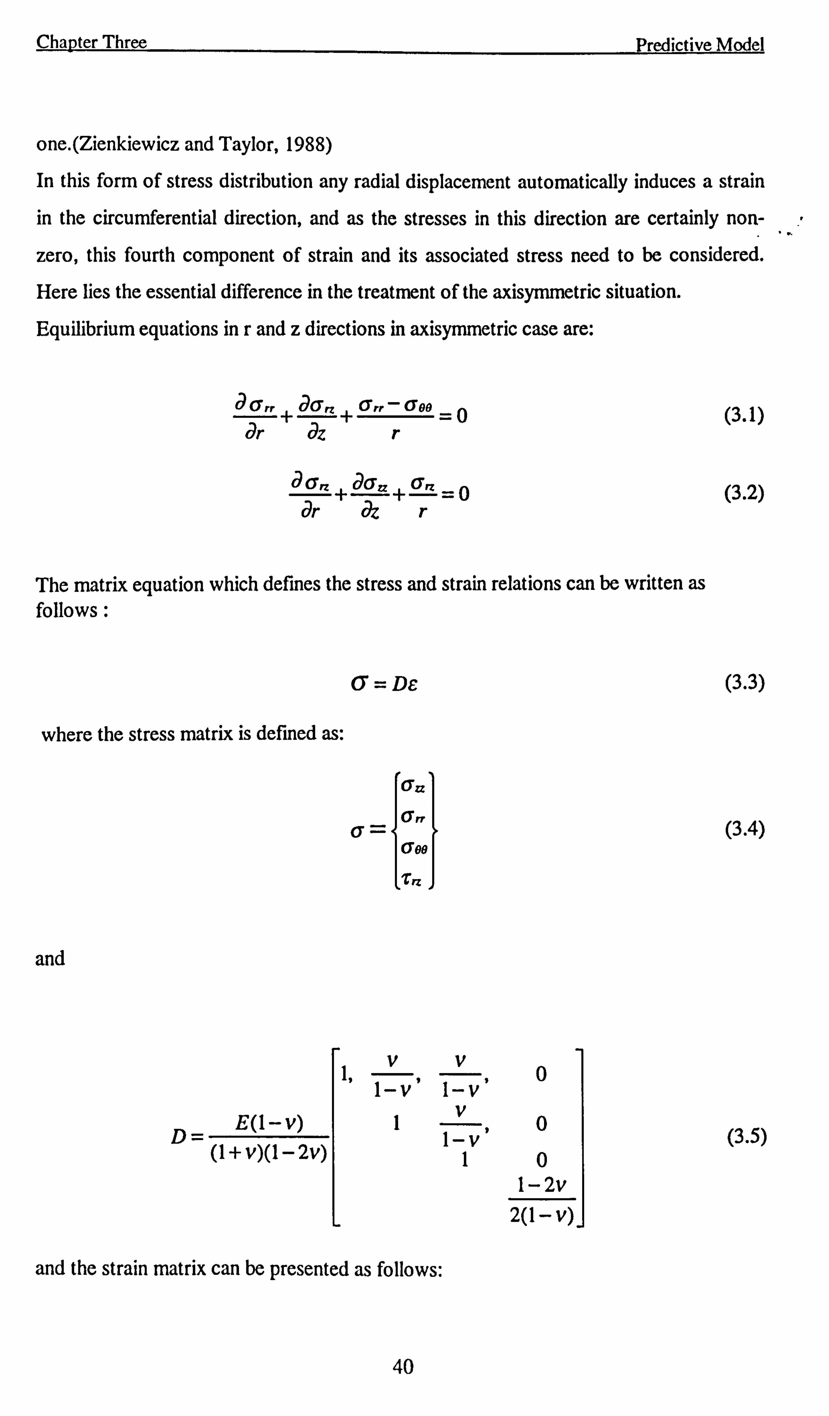
Chapter Three
one. (Zienkiewicz and Taylor, 1988)
In this form of stress distribution any radial displacement automatically induces a strain in the circumferential direction, and as the stresses in this direction are certainly non-
zero, this fourth component of strain and its associated stress need to be considered.
Here lies the essential difference in the treatment of the axisymmetric situation.
Equilibrium equations in r and z directions in axisymmetric case are:
ßrr+aQrz+Qrr-(Tog
=o ar dz r
aa, =+aatt+az ar dz r
The matrix equation which defines the stress and strain relations can be written as follows :
6=DE
where the stress matrix is defined as:
Q=
and
Predictive Model
6u
Qn
Coo
ZR
(3.1)
(3.2)
(3.3)
(3.4)
VVO 1'
1-v' 1-v'
D= E(1 - v)
(1+v)(1-2v) 1y, 0
1-v (3.5) 10
1-2v 2(1-v)
and the strain matrix can be presented as follows:
40
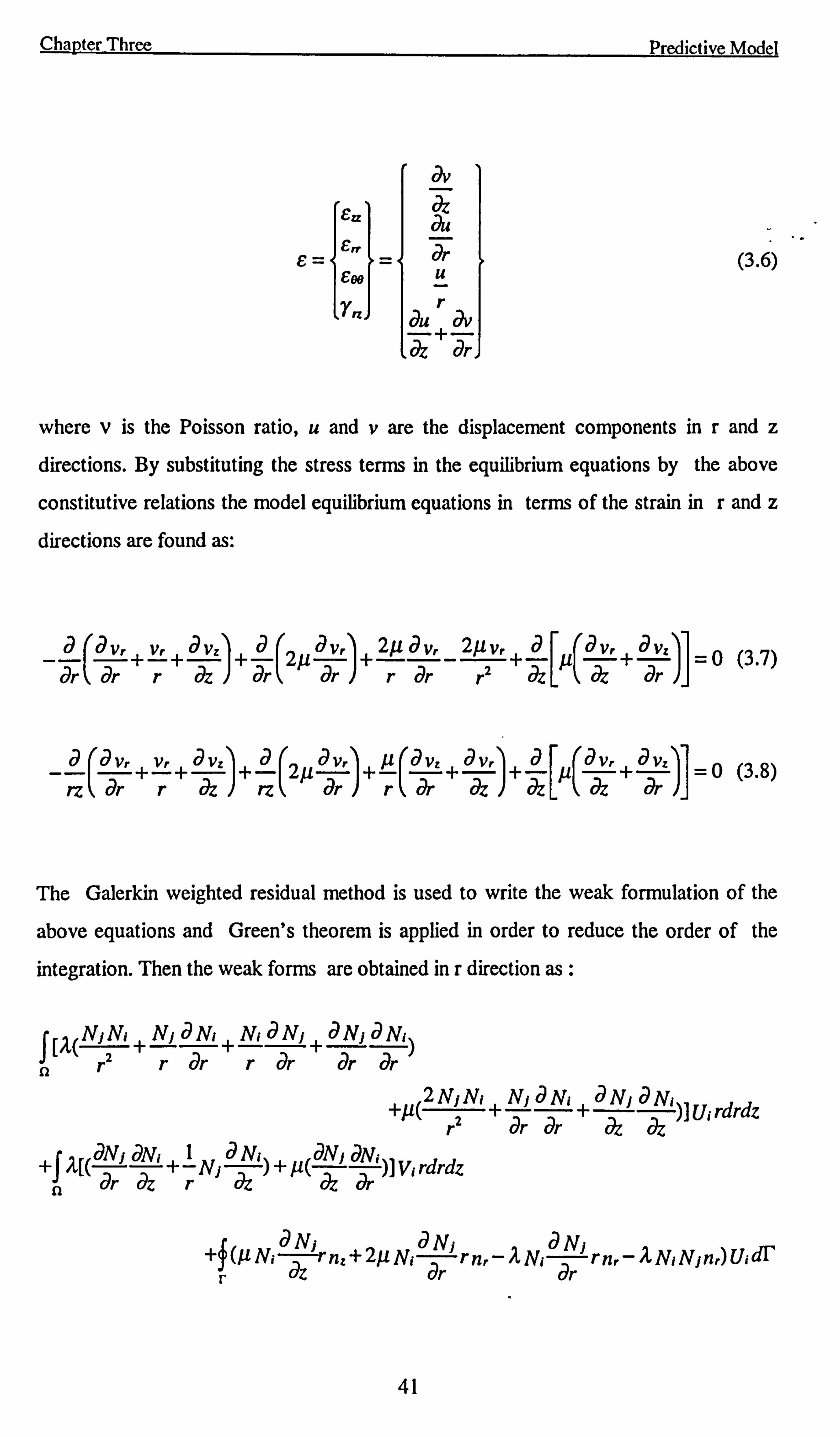
Chapter Three Predictive Model
f Ezz E?
Ego
YR
t)V
öz au
0- u r au av
az + ar
(3.6)
where v is the Poisson ratio, u and v are the displacement components in r and z
directions. By substituting the stress terms in the equilibrium equations by the above
constitutive relations the model equilibrium equations in terms of the strain in r and z
directions are found as:
a av, ý, avz a av, 2µ av, 2µv, av, avZ - +-+ +- 2µ +- - +- µ+
]=O (3.7) Tr
(-aT
r dz ar ar r Tr
r2 dz dz ar
, _a
aVr + V,.
+ aVt
+a 21/ aVrl
+µ-+ avl+ aµa Vr +
2v')] = 0(3.8)
(
ar r dz rz l'
ar l r(. ýOv'
r dz J az dz ar rz l
The Galerkin weighted residual method is used to write the weak formulation of the
above equations and Green's theorem is applied in order to reduce the order of the
integration. Then the weak forms are obtained in r direction as :
f [)(NiNi +N1 äNr+Nr aNf+aNj aNrý
ai- 0 r2 r dr r dr dr
2Nj N; NJ aN; +aNjaN; )l U; rdrdz +µ(
r2 + ar är az ai
aNj äN, 1a Ni) aNj aNi +ýý«
ar dz +r Ni dz +µýaz ar )I Vrrdrdz n
(P rn, -ý, NiaNi rn, -AN, Nin, )Uiý r
dz dr
YR
41
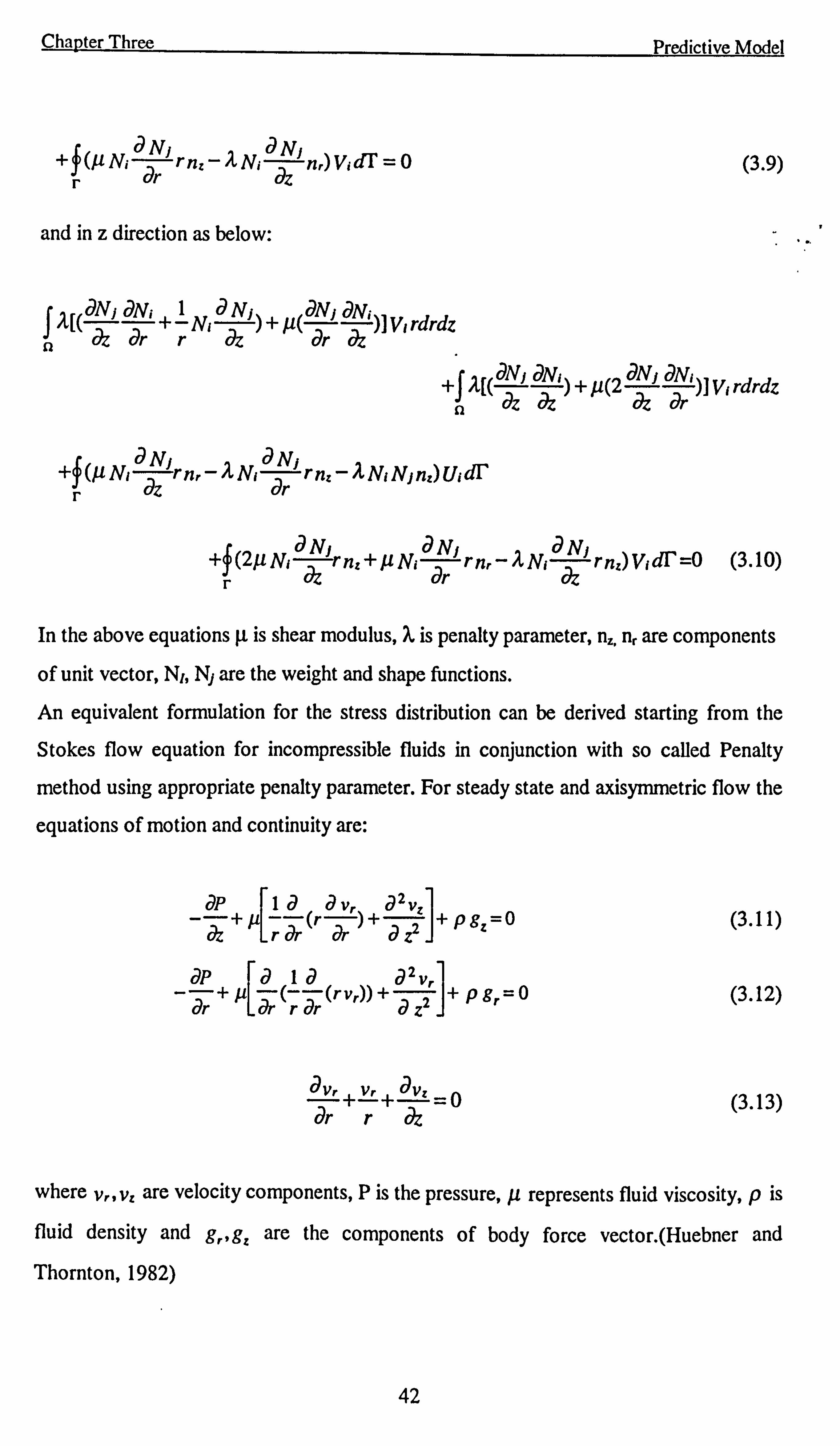
Chapter Three
aNf A
aNJ ý(µN; ar rnZ -N; dz n, )V, ý'=0
r
and in z direction as below:
(aNjaNi +1NjaN; aNiaNr
dz ar r dz )+ µ( ar az
)] V, rdrdz
Predictive Model
(3.9)
aN aN! aNf aNr
+ jýtc aZj ý )+ µ(2
az ý)l Vr rdrdz
n +f (µNraý jrnr-ýNraä jrnZ-ýNsNjn=)UrdI'
r
aNi aNf aNj +f (211 Ni rn=+iuN; rn, -, INr rnZ)Vrdl=O (3.10)
a dr dz r
In the above equations µ is shear modulus, X is penalty parameter, nZ, nr are components
of unit vector, N1, Nj are the weight and shape functions.
An equivalent formulation for the stress distribution can be derived starting from the
Stokes flow equation for incompressible fluids in conjunction with so called Penalty
method using appropriate penalty parameter. For steady state and axisymmetric flow the
equations of motion and continuity are:
aP laav, a2vt az
+µ rar(r ar
)+ az2
+PgL=O
aP alaa2v, ar+µ ar(rar(rv,
))+ a2 j+Pgr Z
avr+vr+avZ
ar r dz
(3.11)
(3.1 Z)
(3.13)
where v,, v, are velocity components, P is the pressure, u represents fluid viscosity, p is
fluid density and g,, g, are the components of body force vector. (Huebner and
Thornton, 1982)
42
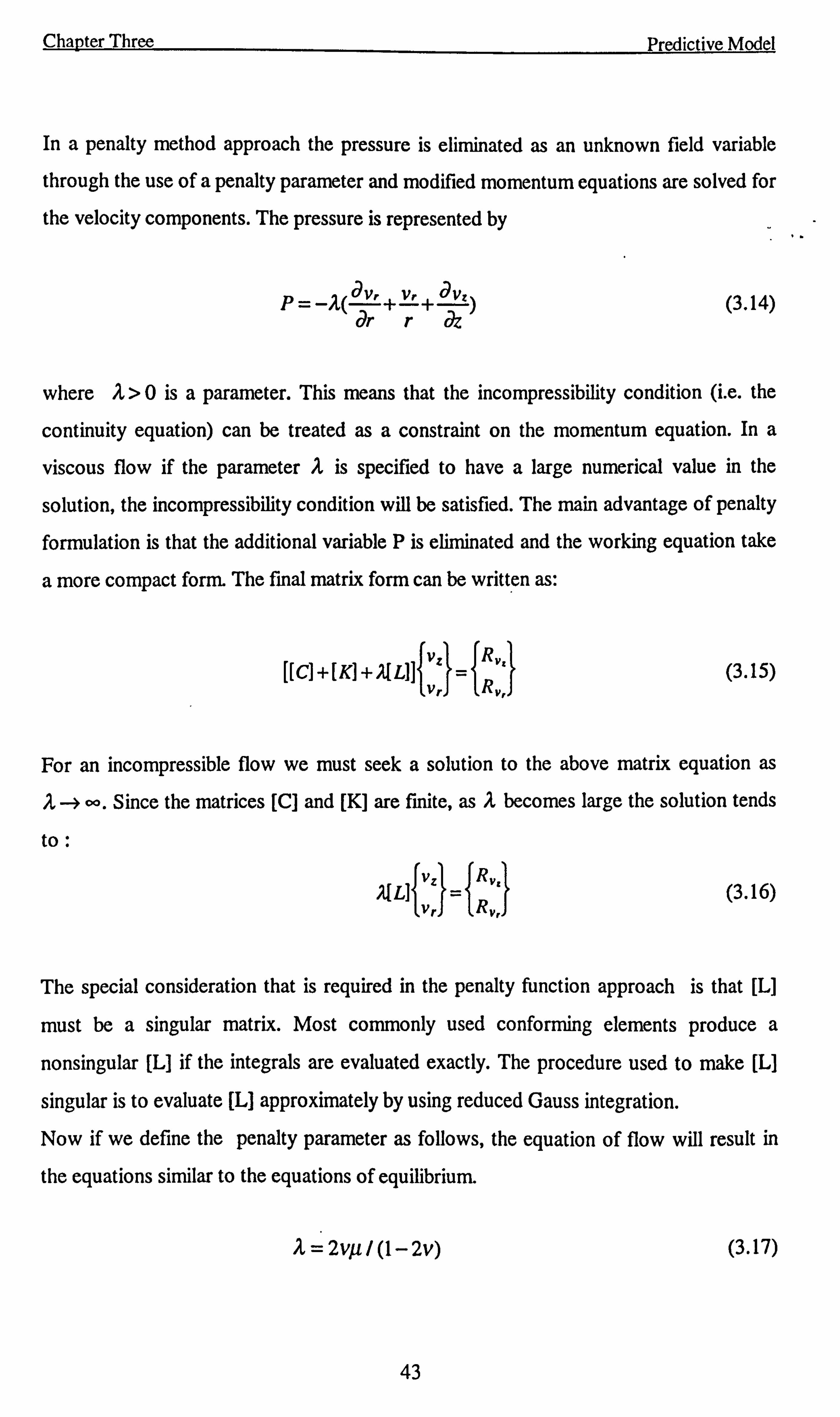
Chapter Three Predictive Model
In a penalty method approach the pressure is eliminated as an unknown field variable
through the use of a penalty parameter and modified momentum equations are solved for
the velocity components. The pressure is represented by
P--/1 aV+Vr+avZ Or r r}z
(3.14)
where A> 0 is a parameter. This means that the incompressibility condition (i. e. the
continuity equation) can be treated as a constraint on the momentum equation. In a
viscous flow if the parameter A is specified to have a large numerical value in the
solution, the incompressibility condition will be satisfied. The main advantage of penalty
formulation is that the additional variable P is eliminated and the working equation take
a more compact form. The final matrix form can be written as:
[[C]+[K]+A[L]] ivZ
= Rv`
vr Rv. (3.15)
For an incompressible flow we must seek a solution to the above matrix equation as
A. -ý ca. Since the matrices [C] and [K] are finite, as A becomes large the solution tends
to .
AjL] Vv,
= Rv, (3.16)
The special consideration that is required in the penalty function approach is that [L]
must be a singular matrix. Most commonly used conforming elements produce a
nonsingular [L] if the integrals are evaluated exactly. The procedure used to make [L]
singular is to evaluate [L] approximately by using reduced Gauss integration.
Now if we define the penalty parameter as follows, the equation of flow will result in
the equations similar to the equations of equilibrium.
ý =2vµl(1-2v) (3.17)
43
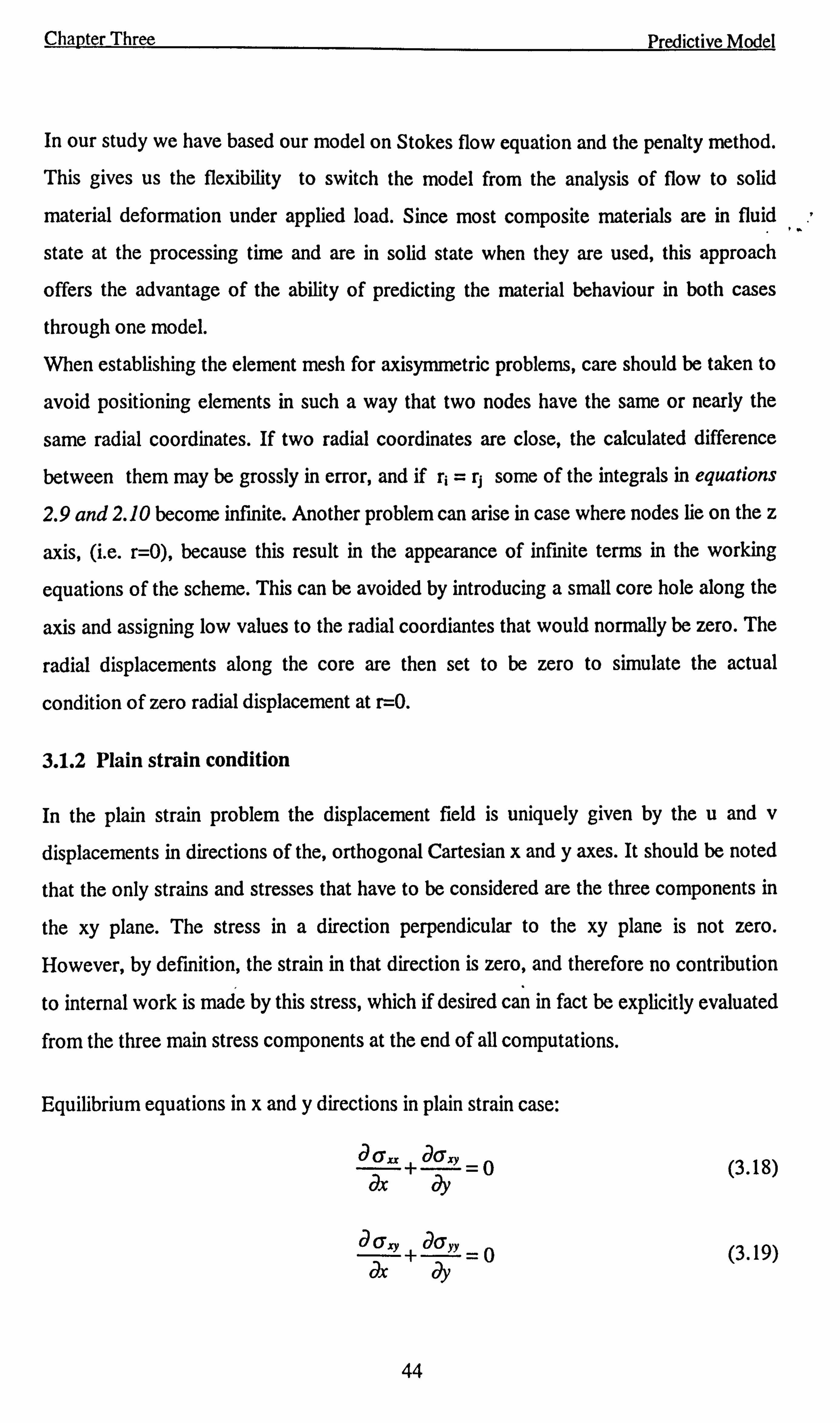
Chapter Three Predictive Model
In our study we have based our model on Stokes flow equation and the penalty method. This gives us the flexibility to switch the model from the analysis of flow to solid
material deformation under applied load. Since most composite materials are in fluid
state at the processing time and are in solid state when they are used, this approach
offers the advantage of the ability of predicting the material behaviour in both cases
through one model.
When establishing the element mesh for axisymmetric problems, care should be taken to
avoid positioning elements in such a way that two nodes have the same or nearly the
same radial coordinates. If two radial coordinates are close, the calculated difference
between them may be grossly in error, and if r; = rj some of the integrals in equations
2.9 and 2.10 become infinite. Another problem can arise in case where nodes he on the z
axis, (i. e. r=0), because this result in the appearance of infinite terms in the working
equations of the scheme. This can be avoided by introducing a small core hole along the
axis and assigning low values to the radial coordiantes that would normally be zero. The
radial displacements along the core are then set to be zero to simulate the actual
condition of zero radial displacement at r=0.
3.1.2 Plain strain condition
In the plain strain problem the displacement field is uniquely given by the u and v
displacements in directions of the, orthogonal Cartesian x and y axes. It should be noted
that the only strains and stresses that have to be considered are the three components in
the xy plane. The stress in a direction perpendicular to the xy plane is not zero.
However, by definition, the strain in that direction is zero, and therefore no contribution
to internal work is made by this stress, which if desired can in fact be explicitly evaluated
from the three main stress components at the end of all computations.
Equilibrium equations in x and y directions in plain strain case:
aý +a6xy dy
aý +aßyy dy
(3.18)
(3.19)
44
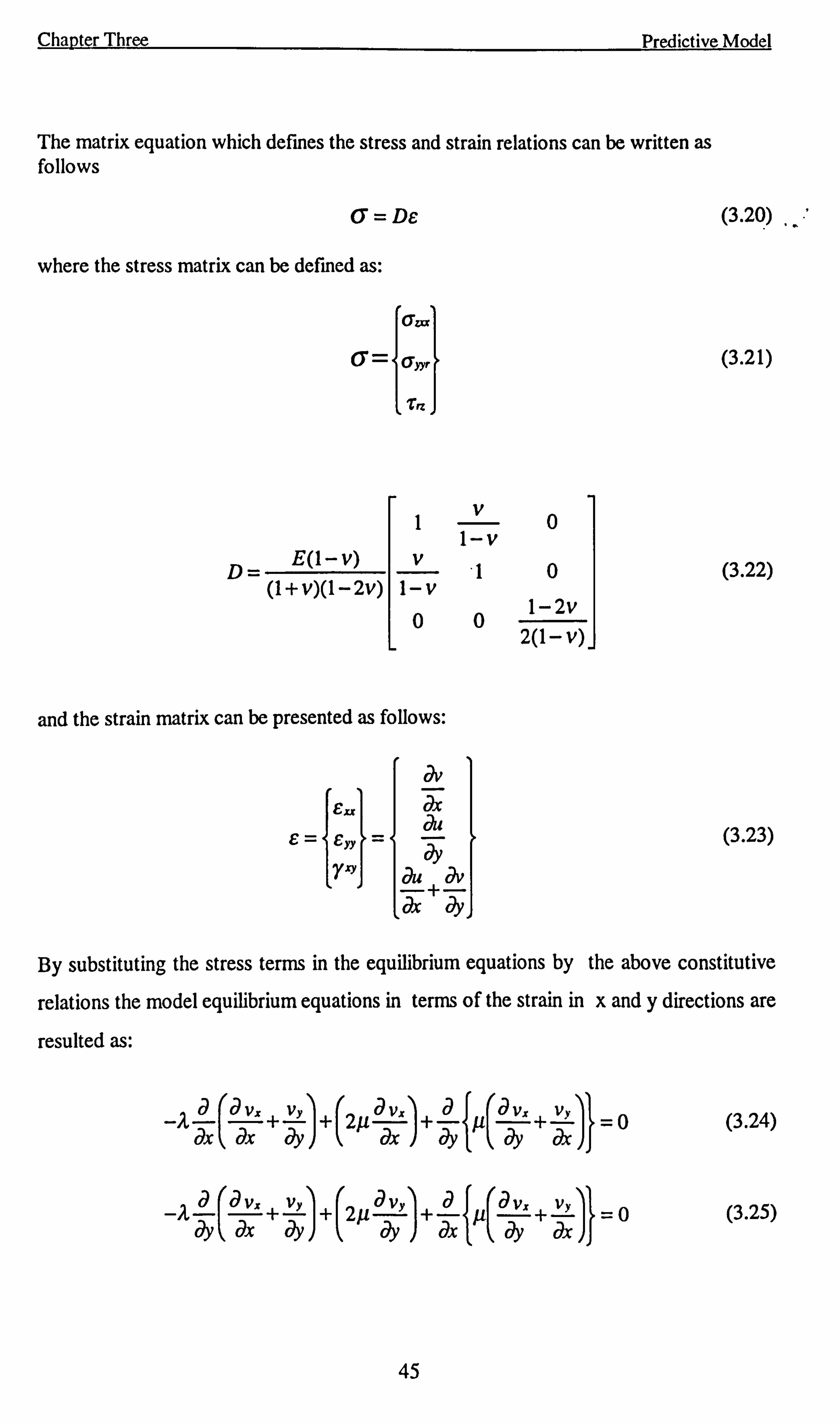
Chapter Three Predictive Model
The matrix equation which defines the stress and strain relations can be written as follows
6=De
where the stress matrix can be defined as:
Uzu
6= 6yy,
zz
D- E(1- v)
(1+v)(1-2v)
(3.20)
(3.21)
1v0 1-v
v10 1-v
(3.22)
00 1-2v 2(1-v)
and the strain matrix can be presented as follows:
,=ý (3.23) dy
au dv az jý
By substituting the stress terms in the equilibrium equations by the above constitutive
relations the model equilibrium equations in terms of the strain in x and y directions are
resulted as:
-a ýý+ vy +(2,4 ý+a lft(-a-vx +ý=0 (3.24)
ý' ý' ý
-A a ý"
+ vy + 29 a vy )+{x+x1 =o (3.25)
aY aY ý' aY
45
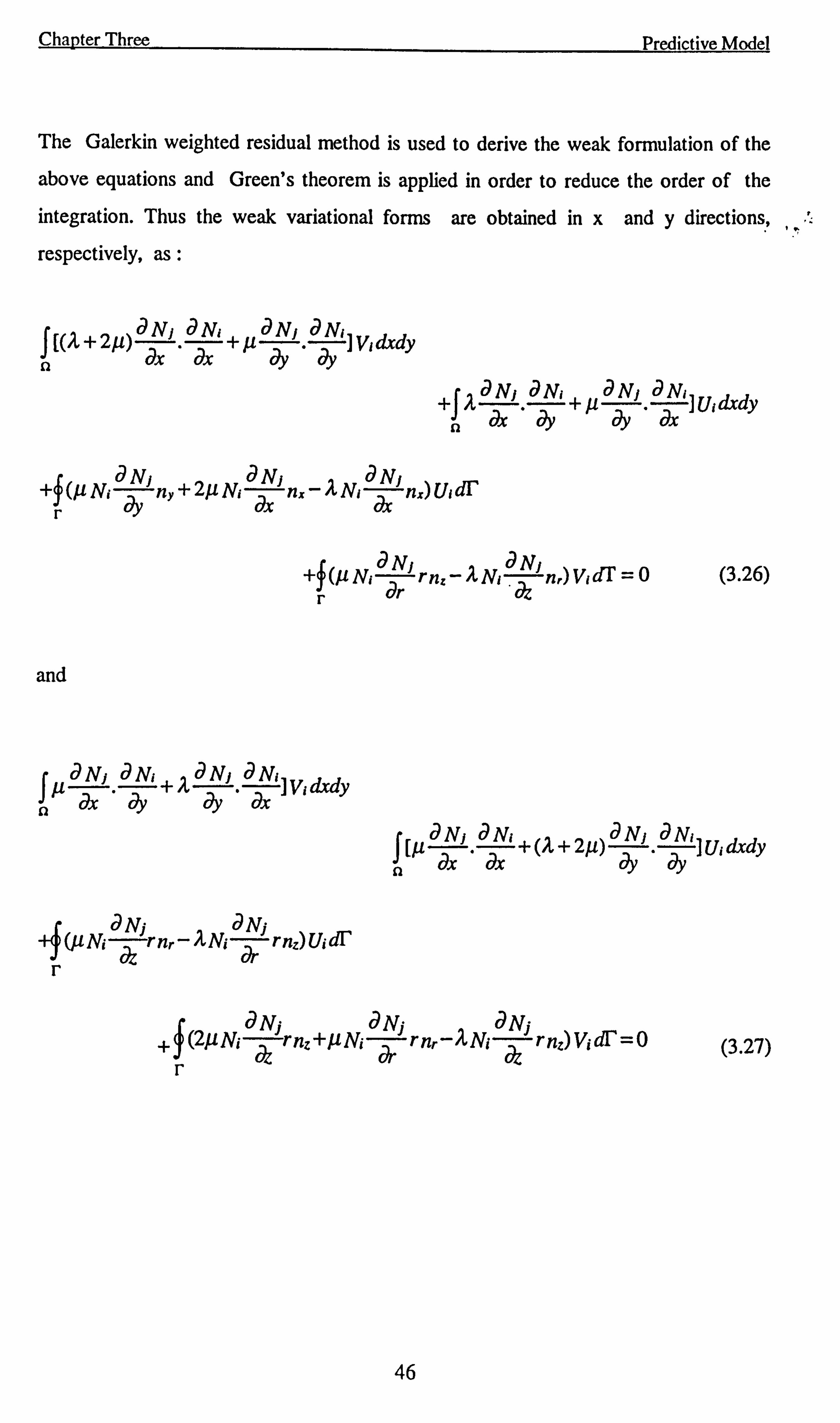
Chapter Three Predictive Model
The Galerkin weighted residual method is used to derive the weak formulation of the
above equations and Green's theorem is applied in order to reduce the order of the
integration. Thus the weak variational forms are obtained in x and y directions,
respectively, as :
f [(ý+2µ) ýJ. ý`+µaNJ. aN']V,
dxdy n
ay dy
+J; t aNi äNr+ aNj aNrI Urdxdy
n az ay u ay ax
+f (11 NraNJny+2µN; ýJnx-A
Ni ýJnx)UrdI'
r ý'
+ý(µNiaa 1 rnZ-, 1 n. )Vrý'=0 (3.26) r
and
Jµ dN' d Ni +ý
d a]
Vi dxdy ayN'
aýN'
ny
-Iý(ý. lNtaNýrnr-ýNi ýýrnz)Uidr'
r az
VI vL
f [ttaNi. ý'+(A,
+2, u)aNJ aN']U;
dxdy n
ay ay
PAM a1Vj
rnz+µNiaNj aNj
rý Trnr-ANi dz rnz)Vidi'=0 (3.27)
46
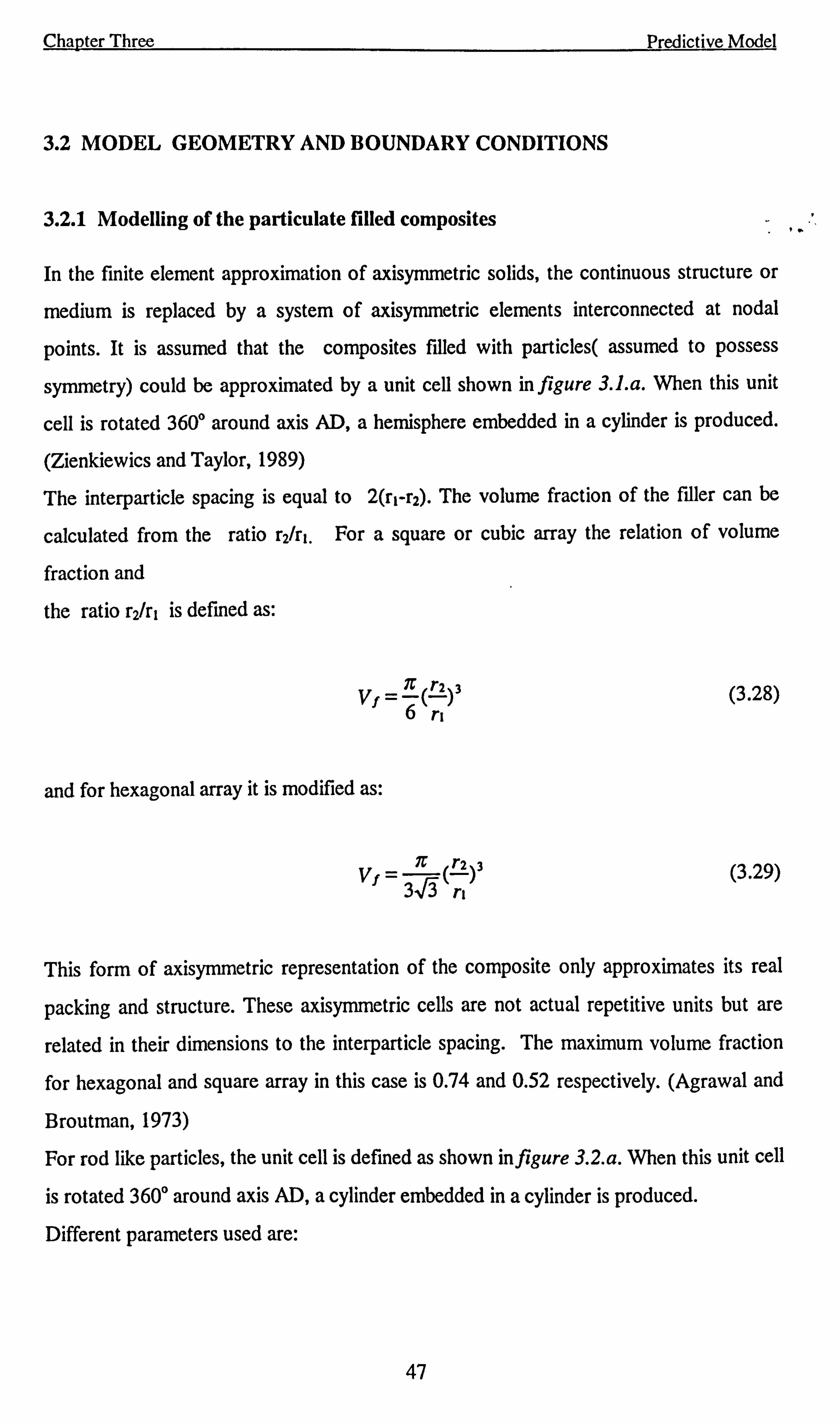
Chapter Three
3.2 MODEL GEOMETRY AND BOUNDARY CONDITIONS
3.2.1 Modelling of the particulate filled composites
Predictive Model
In the finite element approximation of axisymmetric solids, the continuous structure or
medium is replaced by a system of axisymmetric elements interconnected at nodal
points. It is assumed that the composites filled with particles( assumed to possess
symmetry) could be approximated by a unit cell shown in figure 3.1. a. When this unit
cell is rotated 360° around axis AD, a hemisphere embedded in a cylinder is produced.
(Zienkiewics and Taylor, 1989)
The interparticle spacing is equal to 2(ri-r2). The volume fraction of the filler can be
calculated from the ratio r2/r1. For a square or cubic array the relation of volume
fraction and
the ratio r2/rl is defined as:
n r2 3 Vf= 6(rý)
and for hexagonal array it is modified as:
_n rz 3 Vf
3ýýriý
(3.28)
(3.29)
This form of axisymmetric representation of the composite only approximates its real
packing and structure. These axisymmetric cells are not actual repetitive units but are
related in their dimensions to the interparticle spacing. The maximum volume fraction
for hexagonal and square array in this case is 0.74 and 0.52 respectively. (Agrawal and
Broutman, 1973)
For rod like particles, the unit cell is defined as shown in figure 3.2. a. When this unit cell
is rotated 360° around axis AD, a cylinder embedded in a cylinder is produced.
Different parameters used are:
47
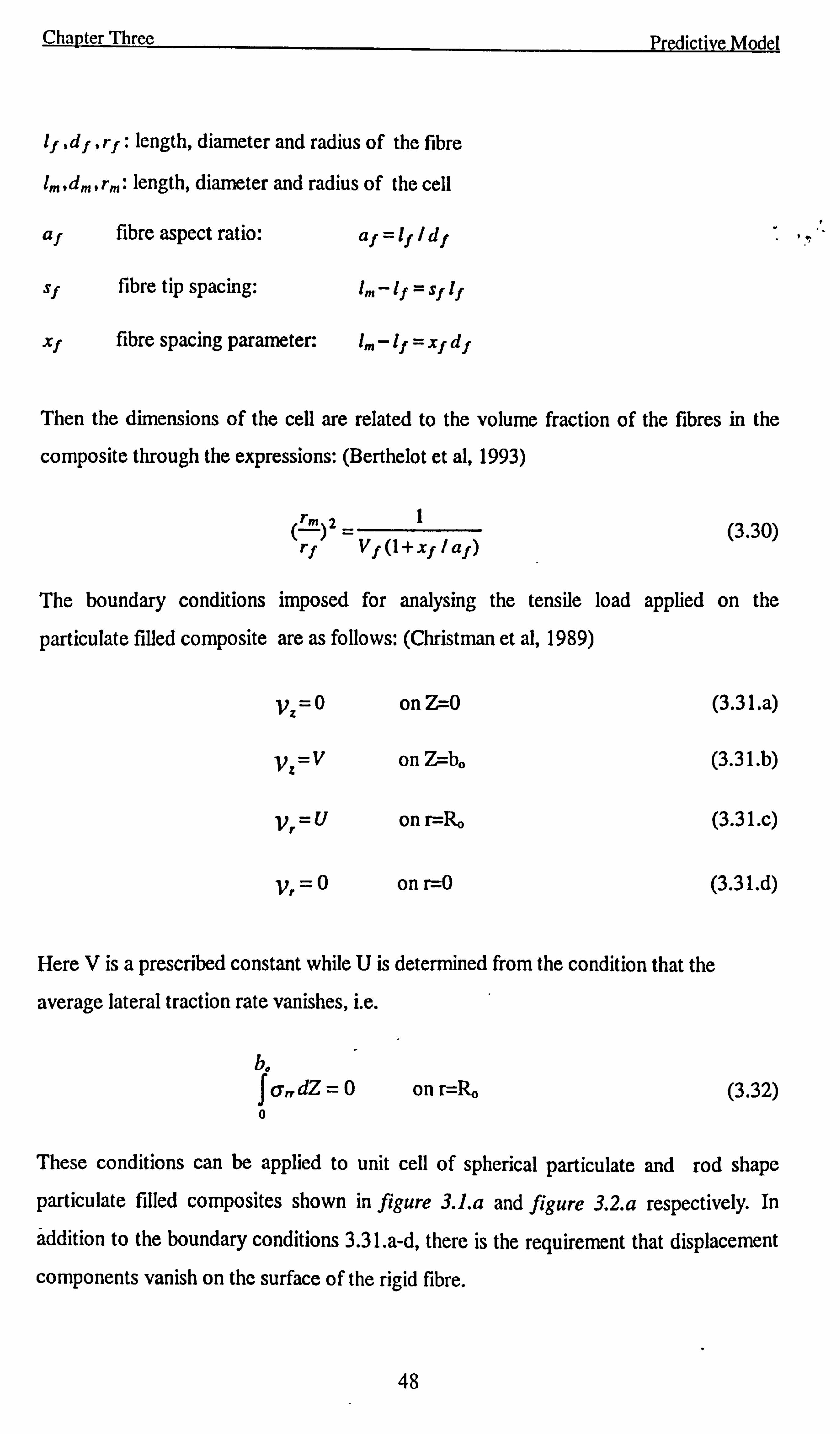
Chapter Three
If ,df, rf: length, diameter and radius of the fibre
1m� dm, r, �: length, diameter and radius of the cell
af
Sf
xI
fibre aspect ratio:
fibre tip spacing:
fibre spacing parameter:
af=lfld f
l, �-if=sflf
l, �-If=zfdf
Predictive Model
Then the dimensions of the cell are related to the volume fraction of the fibres in the
composite through the expressions: (Berthelot et al, 1993)
2_1 (rfr, �) V f(1+xf/af)
(3.30)
The boundary conditions imposed for analysing the tensile load applied on the
particulate filled composite are as follows: (Christman et al, 1989)
VZ =0 on Z=0 (3.31. a)
VZ =V on Z=bo (3.31. b)
Vr =U on r=Ro (3.31. c)
Vr=O on r=0 (3.31. d)
Here V is a prescribed constant while U is determined from the condition that the
average lateral traction rate vanishes, i. e.
b, Jo. dZ=O on r--R. 0
(3.32)
These conditions can be applied to unit cell of spherical particulate and rod shape
particulate filled composites shown in figure 3.1. a and figure 3.2. a respectively. In
addition to the boundary conditions 3.31. a-d, there is the requirement that displacement
components vanish on the surface of the rigid fibre.
48
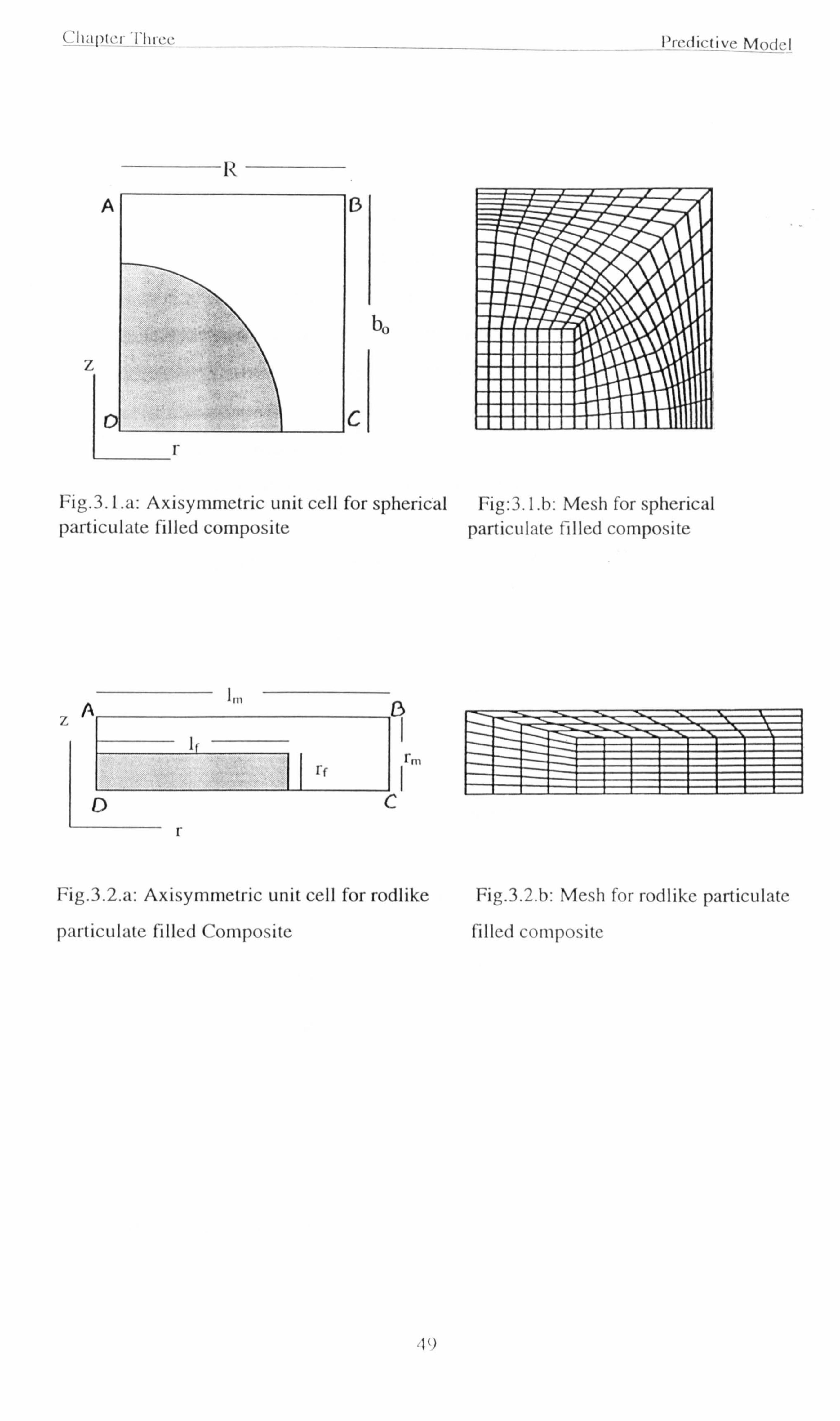
('ir<<l)I'. r_'I'llicc
ýz A
7
C
I-
L3
vo
C
I 'i '(IR IIv'e Model
u,
Fig. 3. La: Axisymmetric unit cell for spherical Fig: 3.1. b: Mesh for spherical particulate filled composite particulate filled composite
1II, 7
II c
F
rm 0
Fig. 3.2. a: Axisymmetric unit cell for rodlike Fig. 3.2. b: Mesh for rodlike particulate
particulate filled Composite filled composite
1O
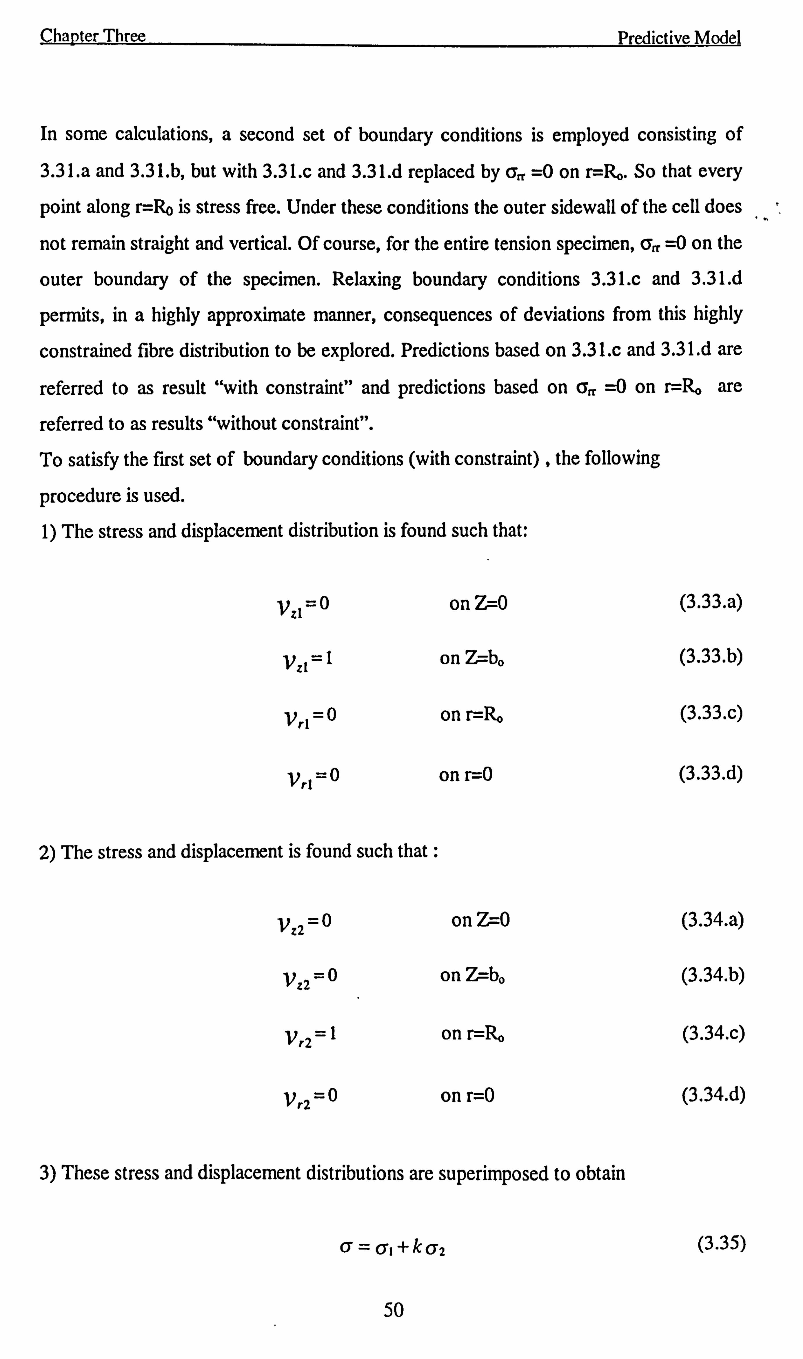
Chapter Three Predictive Model
In some calculations, a second set of boundary conditions is employed consisting of
3.31. a and 3.31. b, but with 3.31. c and 3.31. d replaced by aR =0 on r=R,. So that every
point along r=Ro is stress free. Under these conditions the outer sidewall of the cell does
not remain straight and vertical. Of course, for the entire tension specimen, aR =0 on the
outer boundary of the specimen. Relaxing boundary conditions 3.31. c and 3.31. d
permits, in a highly approximate manner, consequences of deviations from this highly
constrained fibre distribution to be explored. Predictions based on 3.31. c and 3.31 .d are
referred to as result "with constraint" and predictions based on art =0 on r=Ro are
referred to as results "without constraint".
To satisfy the first set of boundary conditions (with constraint) , the following
procedure is used.
1) The stress and displacement distribution is found such that:
vz, =0 on Z--0 (3.33. a)
vzt =1 on Z--b. (3.33. b)
vr, =0 on r=Ro (3.33. c)
vr1= 0 on r=0 (3.33. d)
2) The stress and displacement is found such that :
vz2 =0 on Z--0 (3.34. a)
vz2 =0 on Z-- bo (3.34. b)
vr2 =1 on r=Ro (3.34. c)
Vr2 =0 on r=0 (3.34. d)
3) These stress and displacement distributions are superimposed to obtain
6=a, +k 62 (3.35)
50
Chapter Three
and v=Vl+kV2 (3.36)
where k is determined such that the net force in the r direction along be is zero.
(Agrawal et al , 1971) thus
(Fr) BC -f (a,, +k (Tr2)dZ = IBCJ(6º1 +k ar2) BC =0 BC
so that r1 k=(2
Qr2 BC
The stress on AB is thus
\QL/AB - l6zIJAB -
ßrl (6z2)AB
ar2 BC
and the displacement is
(uz)AB -
(uz1)AB ßrl2
BC
(UZ2)AB -
(UZI)AB
Qr
since (UZ2)AB =0.
3.2.2 Fibre reinforced composite
(3.37)
(3.38)
(3.39)
(3.40)
The plain strain analysis can be used for the fibre reinforced composite. Figure 3.3. a
shows the unit cell for the cubic array configuration of fibre reinforced composite. The
following expression defines the relation between the unit cell dimensions and the
volume fraction:
Vf= 7i 4r
r2
l (3.41)
Figure 3.4. a shows the unit cell employed for 'the hexagonal array configuration.
Numerous choices exist for the unit cell geometry. The unit cell tested is rectangular in
Predictive Model
51
Chapter Three Predictive Model
shape with dimension 2L1*2L2, with L2 = NF3 L1. Then the volume fraction of the fibres
is related to the cell geometry according to
nR3 Vf=V(L) (3.42)
The maximum volume fractions for the square and hexagonal array in the fibre
reinforced composite analysis are 0.907 and 0.785 respectively. (Gibson, 1994)
Using the square array and hexagonal unit cells the composite response to transverse
tensile and shear loading is examined.
2.2.1.1 Tensile loading
The boundary conditions imposed for analysing the tensile load applied on the fibre
reinforced composite are as follows:
vy =0 on y=0 (3.43. a)
vy =V on y--Yo (3.43. b)
Vx =U on x=Xo (3.43. c)
Vx =0 on x=0 (3.43. d)
Here V is a prescribed constant while U is determined from the condition that the
average lateral traction rate vanishes, i. e.
b. 1 Qxxdy =0 on x=Xo (3.44) 0
These conditions can be applied to unit cell of square and hexagonal array of fibre
reinforced composites shown infgure 3.3. a and figure 3.4. a.
52
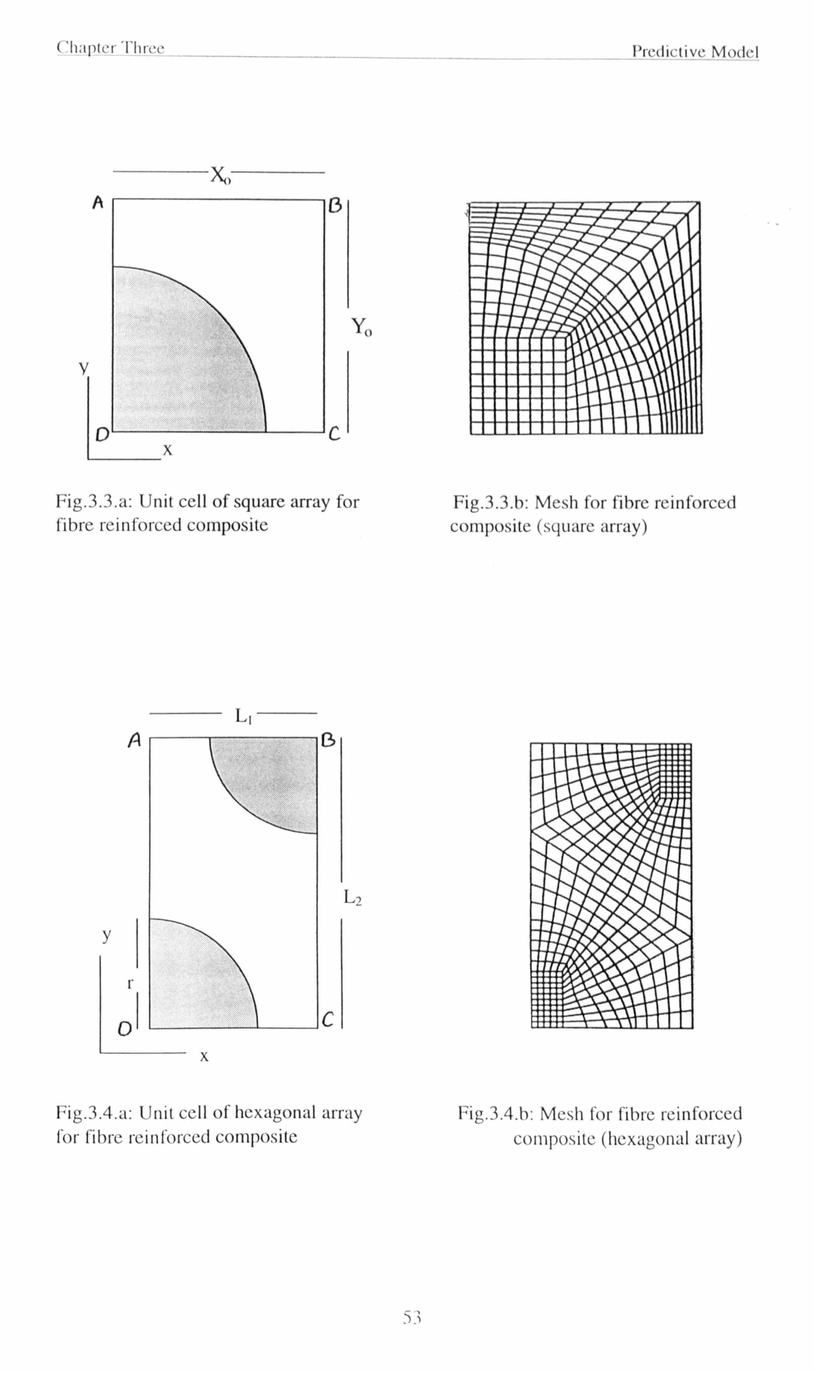
('Iril)lrr'I'l it
`4i
A 13
Y�
v
0 x
C
Fig. 3.3. a: Unit cell of square array for fibre reinforced composite
I..,
�1 13
[_,
Y
0 ý\
x
C
I'rrýlirlivi' Mýx1ý I
- - Fig. 3.3. b: Mesh for fibre reinforced composite (square array)
Fig. 3.4. a: Unit cell of hexagonal array Fig. 3.4. h: Mesh for fibre reinforced for fibre reinforced composite composite (hexagonal array)
Chapter Three Predictive Model
In addition to the boundary conditions 3.31. a-d, there is the requirement that
displacement components vanish on the surface of the rigid fibre.
3.2.2.2 Shear loading
The response of the fibre reinforced composite to transverse shear load is simulated with
the following boundary conditions imposed on the unit cells shown in figure 3.3. a or
figure 3.4. a:
vy=o vx_0
on y=0 (3.45. a)
vx =V on y--Yo (3.45. b)
Vr=0 on x=Xý (3.45. c)
vy =0 on x=0 (3.45. d)
Here V is a prescribed constant in addition to the boundary conditions 3.31 . a-d, there is
the requirement that displacement components vanish on the surface of the rigid
fibre. (Eischen and Torquato, 1993)
3.2.3 Slip boundary conditions
When there is no slip at the interface of the matrix and filler, the relative displacement of
the two phases is the same as zero. Whereas in the case of slip the relative displacement
of the two phase is not zero and the boundary condition is described by Naviers slip
relation, which is a third kind (Robin or convective) boundary condition:
(ßr. n+v). t= 0 (3.46)
Complementary with the above boundary condition is the following relation which
ensures there is no relative radial displacement of the two phase.
vn=0 (3.47)
I.
54
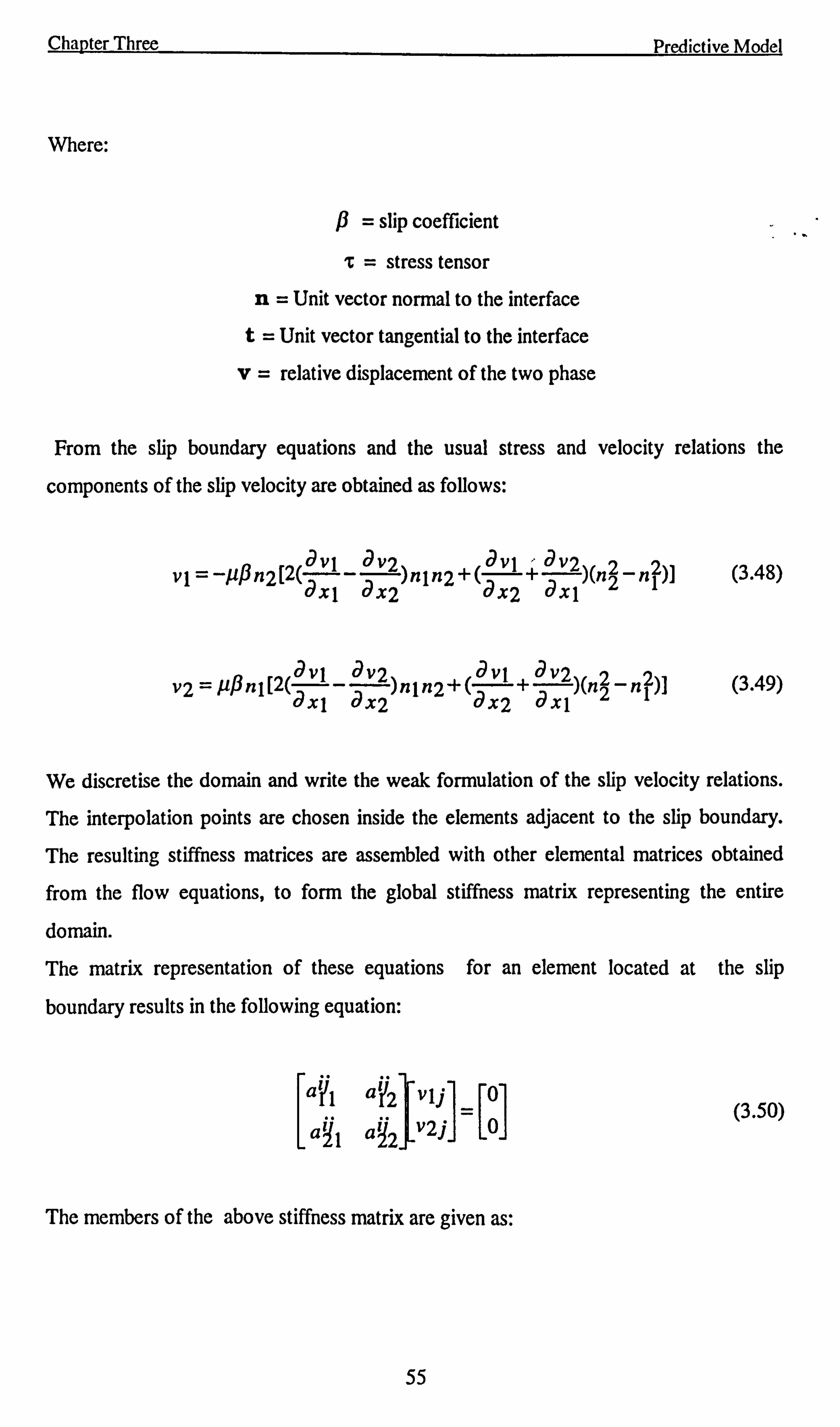
Chapter Three
Where:
ß= slip coefficient
ti = stress tensor
n= Unit vector normal to the interface
t= Unit vector tangential to the interface
v= relative displacement of the two phase
Predictive Model
From the slip boundary equations and the usual stress and velocity relations the
components of the slip velocity are obtained as follows:
19v1 _
av2 avl - av2 v1=-µßn2[2(ax1 ax2)n1n2+(ax2 + ax1)in2-nl)]
_ avl
_ av2 avl av2 v2 - µßnl[2(axl ax2)nln2+(ax2 + axl)(n2 -nl )l
(3.48)
(3.49)
We discretise the domain and write the weak formulation of the slip velocity relations.
The interpolation points are chosen inside the elements adjacent to the slip boundary.
The resulting stiffness matrices are assembled with other elemental matrices obtained
from the flow equations, to form the global stiffness matrix representing the entire
domain.
The matrix representation of these equations for an element located at the slip
boundary results in the following equation:
aIl a12 v1j 0
aql aY2 v2j 0
The members of the above stiffness matrix are given as:
(3.50)
55
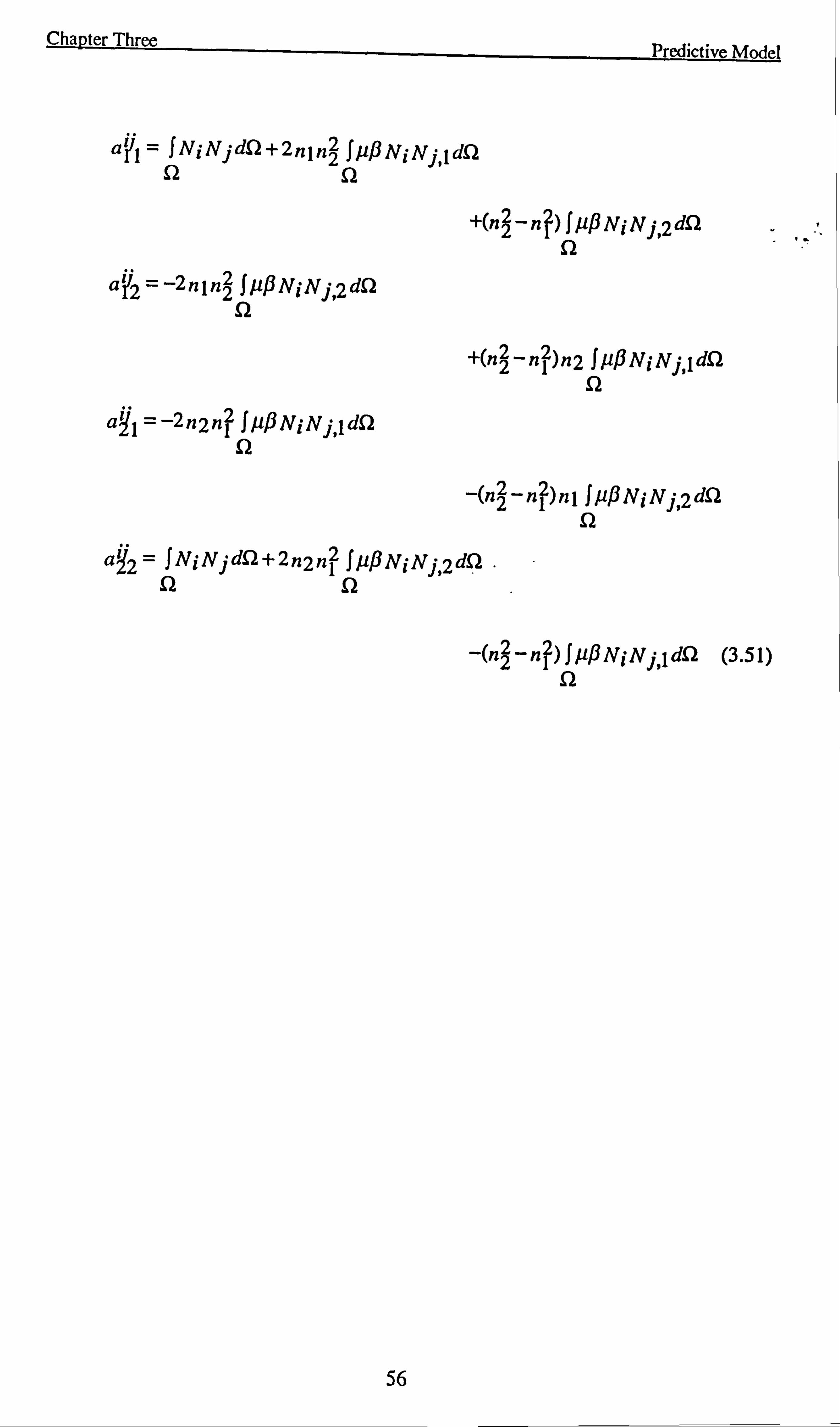
Chapter Three
aV1 =ýNINjdS2+2n1n2 f, ußNiNj, 1dS2 Q
Predictive Model
+(n 2- ný)1 uQ Ni N j, 2 dSZ
aV2=-2n1n2 JußNiNl, 2dS2 S2
+(n2-ni)n2 JµßNiNj, 1dSZ S2
ay1=-2n2n1 f µ/3NjN. j, 1dS2
-(n2-ni)n1 JµßNiNj, 2dS2 S2
aZ2 =ýNiNjdS2+2n2n1 ýµßNiNj,
'(n2'ni)jýßNiN. 1,1dS2 (3.51) 92
56
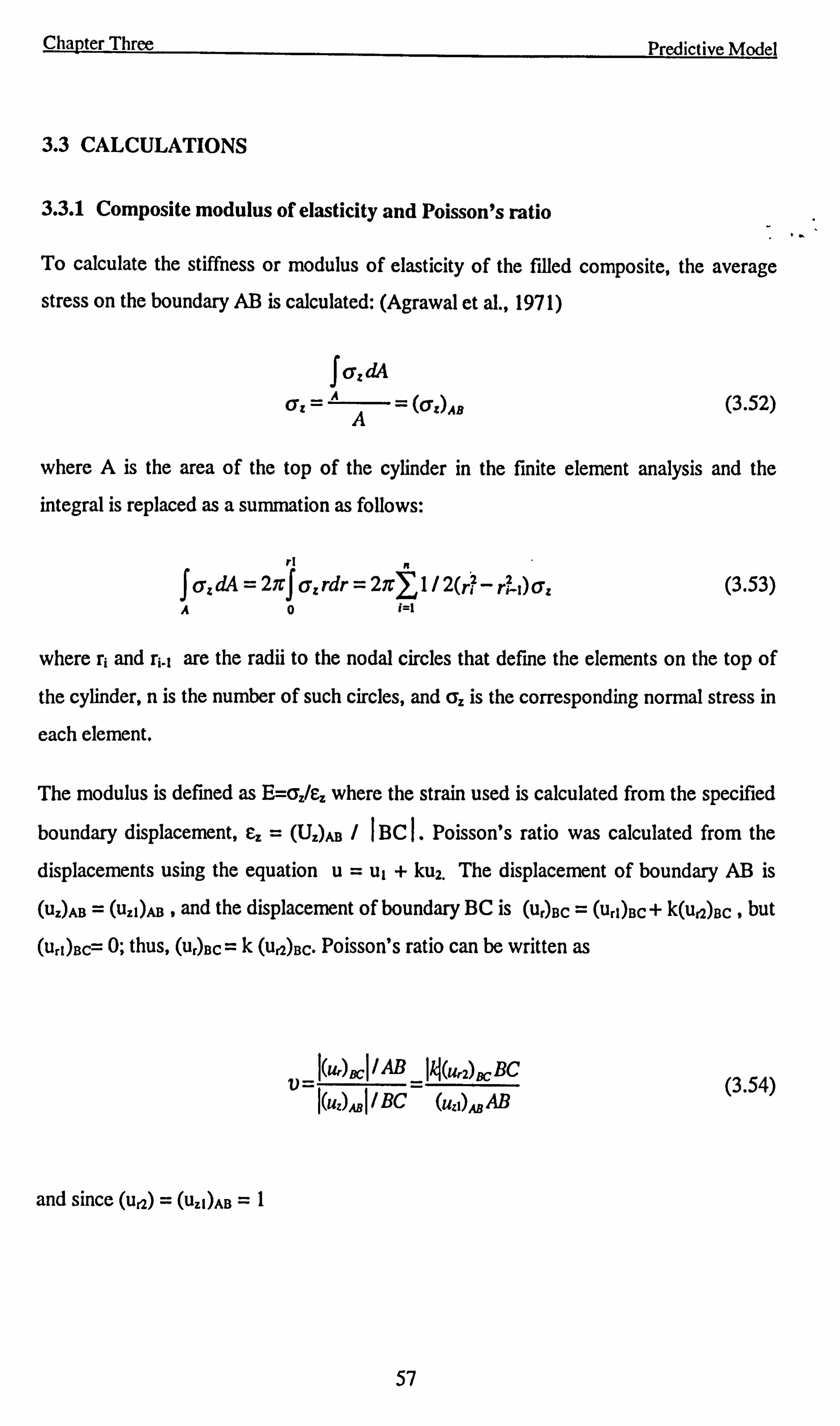
Chapter Three Predictive Model
3.3 CALCULATIONS
3.3.1 Composite modulus of elasticity and Poisson's ratio
To calculate the stiffness or modulus of elasticity of the filled composite, the average
stress on the boundary AB is calculated: (Agrawal et al., 1971)
Ja=d4 A Q= =A= (Q: )Aa (3.52)
where A is the area of the top of the cylinder in the finite element analysis and the
integral is replaced as a summation as follows:
rl e f QZdA=2n f ßZrdr=2nE 1/2(ri-rr-1)Q: A0 ! =1
(3.53)
where r; and r1.1 are the radii to the nodal circles that define the elements on the top of
the cylinder, n is the number of such circles, and aZ is the corresponding normal stress in
each element.
The modulus is defined as E=aZ/e. where the strain used is calculated from the specified
boundary displacement, sZ = (UZ)AB BC I. Poisson's ratio was calculated from the
displacements using the equation u= ul + ku2. The displacement of boundary AB is
(uZ)AB = (uz1)AB , and the displacement of boundary BC is (Ur)BC = (url)BC+ k(u, 2)BC , but
(ur, )Bc= 0; thus, (Ur)BC= k (ui2)BC. Poisson's ratio can be written as
v= I (Ur)BCI l AB
_I M(Ur2)BCBC l(UZ)ABI l BC (uzl)AB AB
(3.54)
and since (un) _ (uZI)AB =I
57
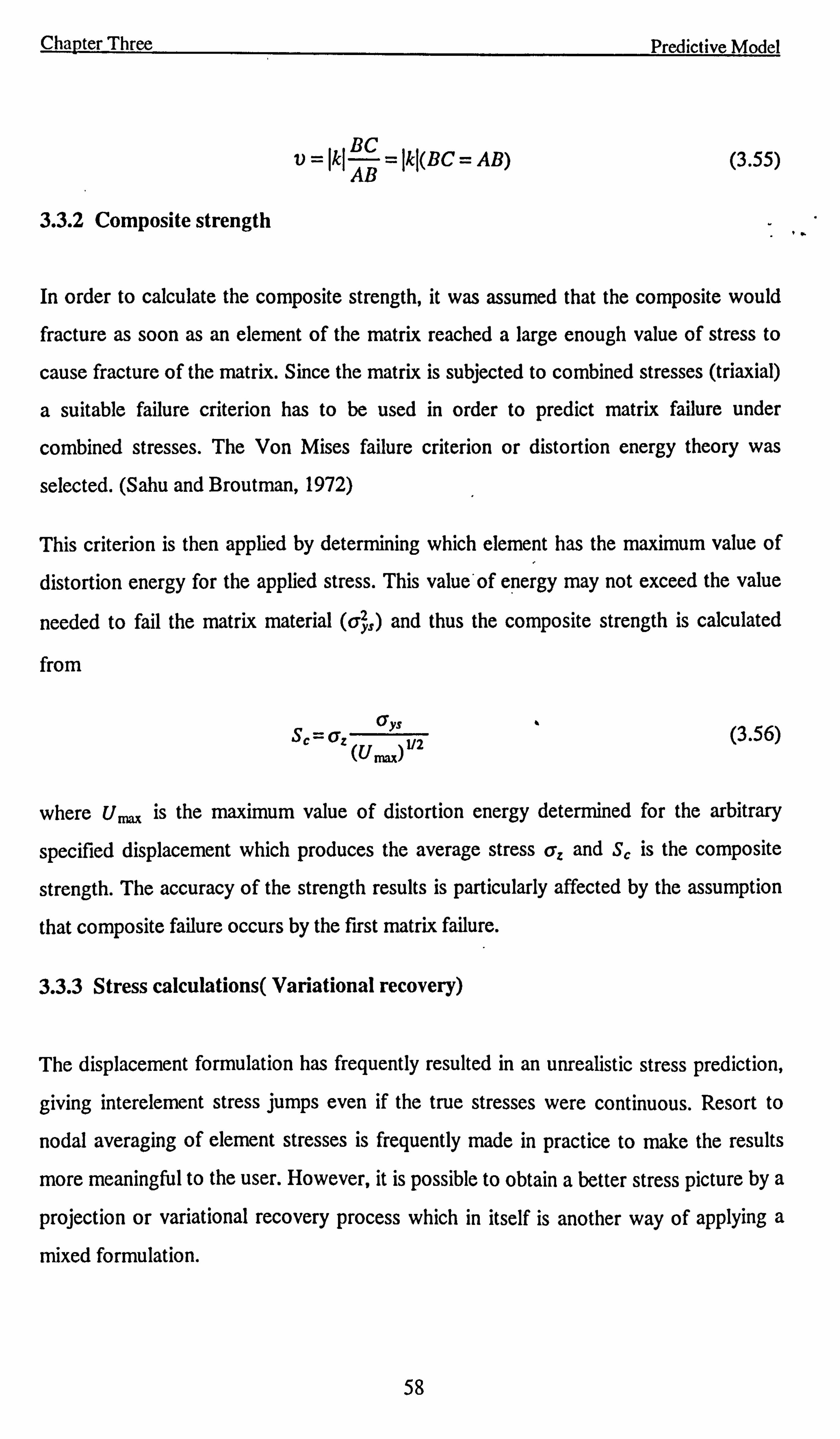
Chapter Three
v- (ký AB - Jkj(BC = AB)
3.3.2 Composite strength
Predictive Model
(3.55)
In order to calculate the composite strength, it was assumed that the composite would
fracture as soon as an element of the matrix reached a large enough value of stress to
cause fracture of the matrix. Since the matrix is subjected to combined stresses (triaxial)
a suitable failure criterion has to be used in order to predict matrix failure under
combined stresses. The Von Mises failure criterion or distortion energy theory was
selected. (Sahu and Broutman, 1972)
This criterion is then applied by determining which element has the maximum value of
distortion energy for the applied stress. This value'of energy may not exceed the value
needed to fail the matrix material (a') and thus the composite strength is calculated
from
Sc =6Z ßys
v2 (Uý) (3.56)
where U is the maximum value of distortion energy determined for the arbitrary
specified displacement which produces the average stress a and S, is the composite
strength. The accuracy of the strength results is particularly affected by the assumption
that composite failure occurs by the first matrix failure.
3.3.3 Stress calculations( Variational recovery)
The displacement formulation has frequently resulted in an unrealistic stress prediction,
giving interelement stress jumps even if the true stresses were continuous. Resort to
nodal averaging of element stresses is frequently made in practice to make the results
more meaningful to the user. However, it is possible to obtain a better stress picture by a
projection or variational recovery process which in itself is another way of applying a
mixed formulation.
58
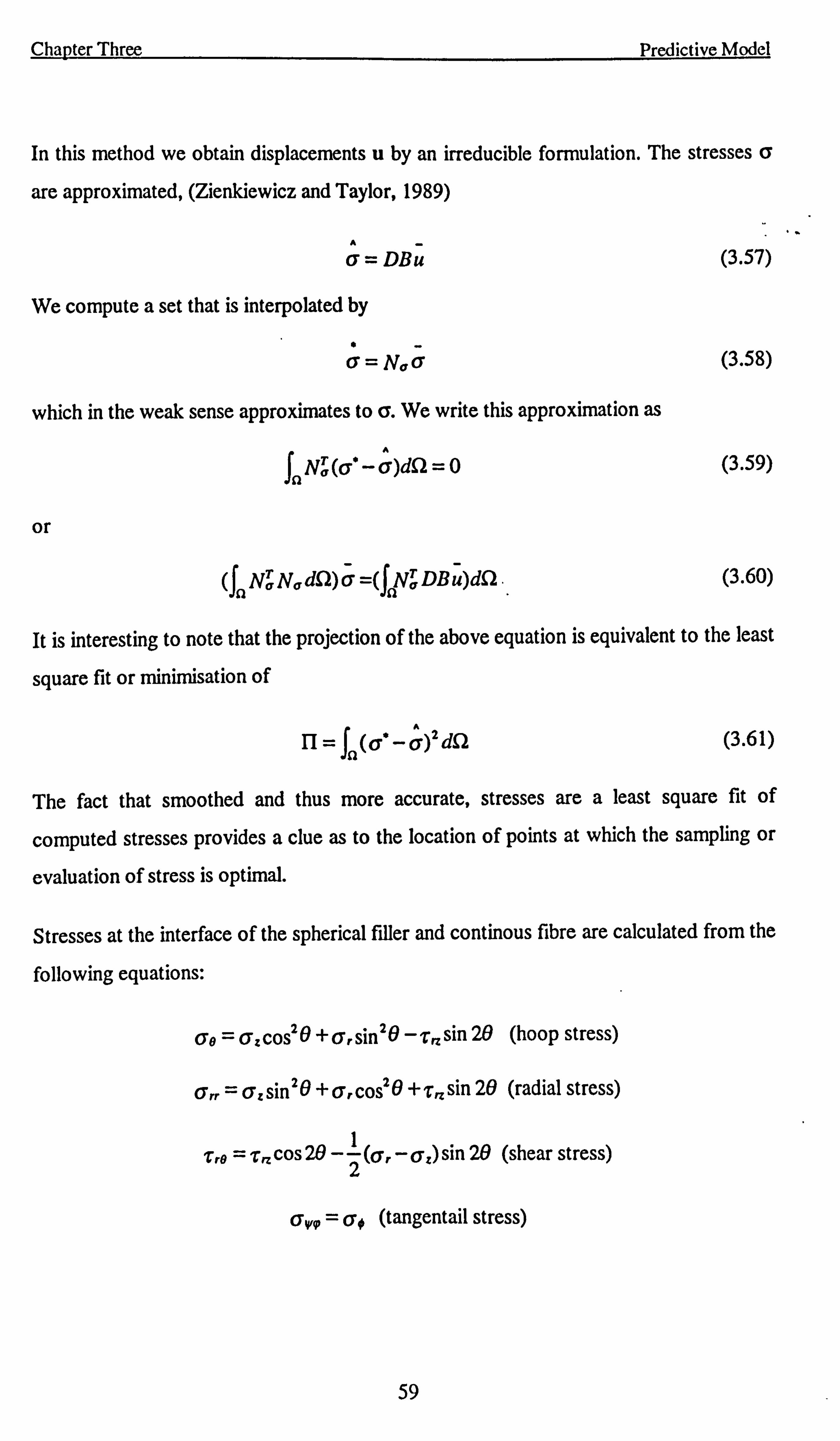
Chapter Three Predictive Model
In this method we obtain displacements u by an irreducible formulation. The stresses a
are approximated, (Zienkiewicz and Taylor, 1989)
6= DBu (3.57)
We compute a set that is interpolated by
a= NQ a (3.58)
which in the weak sense approximates to a. We write this approximation as
faN f -Q)di2=0
or
(3.59)
(JnNäNQdS )6=(fýNQDBu)dfl. (3.60)
It is interesting to note that the projection of the above equation is equivalent to the least
square fit or minimisation of
II - fn(Q -Q)2dS2 (3.61)
The fact that smoothed and thus more accurate, stresses are a least square fit of
computed stresses provides a clue as to the location of points at which the sampling or
evaluation of stress is optimal.
Stresses at the interface of the spherical filler and continous fibre are calculated from the
following equations:
CFO = QzCOS20 +a, sin20 -T, z sin 20 (hoop stress)
a� = aZ sin 20+ Cr cost 0+ zR sin 20 (radial stress)
T rO = 'Crt cos 20 -2 (o
- Qz) sin 20 (shear stress)
6Wm = a'# (tangentail stress)
59
Chapter Four
RESULTS AND DISCUSSION
INTRODUCTION
In this chapter the numerical analysis results are presented and the following topics are
discussed:
" Modulus of composites
A general review of modulus of composites found by numerical analysis and other
methods is presented. The strengths, weaknesses and assumptions made in different
methods are discussed and compared.
" Composites filled with rigid particles
The imposition of the tensile load on a composite filled with particles much stiffer than
the matrix is simulated. The modulus, stress distribution and the strength of these types
of composites are predicted. The tensile stress obtained by our model is compared
with the Papanicolaou model which includes the effects of taking the particle diameter
Chapter Four Results And Discussion
into account. The tensile strengths predicted by different models are compared with the
outcome of our model.
" Composites filled with debonded rigid particles Composites with a weak interface between the filler and matrix which are susceptible
to interfacial crack formation are studied. This condition can be distinguished as
partially bonded inclusion. Another case arises when there is no bonding between the
inclusion and the matrix. In this latter case the slip boundary condition is imposed on
the section of the interface which remains closed. The state of stress and displacement
fields are obtained for both cases. The location of any further deformation through
crazing or shear band formation is identified as a crack tip. Completely unbonded
inclusion with the partial slip at a section of the interface reduces the concentration of
the stress at the crack tip.
The effect of debonding on the strength of the composite is studied.
" Composites filled with soft particle
The behaviour of the rubber filled composites under the tensile load is studied. The
effect and the importance of the use of different filler properties on the outcome of
the numerical analyses are discussed. Two types of toughening mechanisms, namely
shear banding and cavitation, are identified and the fracture behaviour of the
composites is studied.
" Continuous fibre reinforced composites
The responses of the fibre reinforced composites under tensile and shear loads are
investigated. The Young's modulus and shear modulus are calculated. The stress
distribution at interface and throughout the matrix is analysed. Different failure modes
are defined and discussed.
" Short fibre reinforced composite
The effect of different geometrical parameters such as aspect ratio and fibre spacing on
the modulus of the short fibre reinforced composites is examined. The critical fibre
61
Chapter Four Results And Discussion
length for achieving the maximum reinforcement is described. The interfacial shear and
tensile stress are predicted and compared with the shear lag and modified shear lag
models. The model equations are modified by considering the boundary flux terms.
The model predictions for the composite properties and stress fields are obtained with
and without boundary fluxes. The possibility of the composite failure either by
interfacial debonding and fibre breakage is investigated.
62
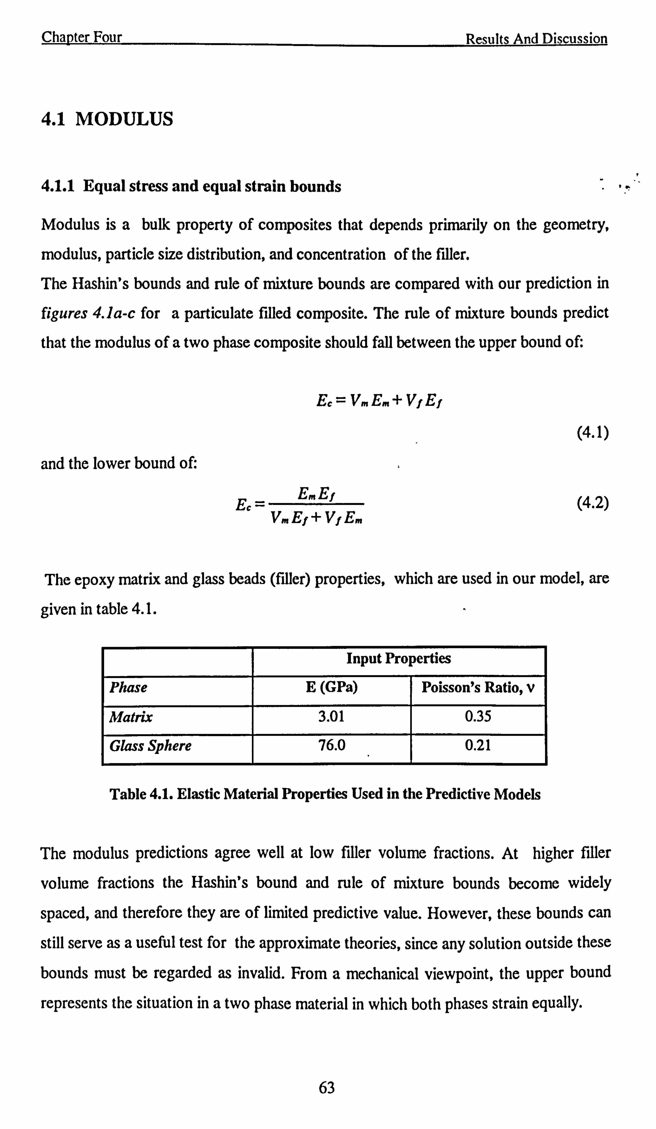
Chapter Four Results And Discussion
4.1 MODULUS
4.1.1 Equal stress and equal strain bounds
Modulus is a bulk property of composites that depends primarily on the geometry,
modulus, particle size distribution, and concentration of the filler.
The Hashin's bounds and rule of mixture bounds are compared with our prediction in
figures 4.1 a-c for a particulate filled composite. The rule of mixture bounds predict
that the modulus of a two phase composite should fall between the upper bound of.
E, =VmEm+VfEf
and the lower bound of.
E, � Ef E, _
V, �Ef+VfE, �
(4.1)
(4.2)
The epoxy matrix and glass beads (filler) properties, which are used in our model, are
given in table 4.1.
Input Properties
Phase E (GPa) Poisson's Ratio, v
Matrix 3.01 0.35
Glass Sphere 76.0 0.21
Table 4.1. Elastic Material Properties Used in the Predictive Models
The modulus predictions agree well at low filler volume fractions. At higher filler
volume fractions the Hashin's bound and rule of mixture bounds become widely
spaced, and therefore they are of limited predictive value. However, these bounds can
still serve as a useful test for the approximate theories, since any solution outside these
bounds must be regarded as invalid. From a mechanical viewpoint, the upper bound
represents the situation in a two phase material in which both phases strain equally.
63
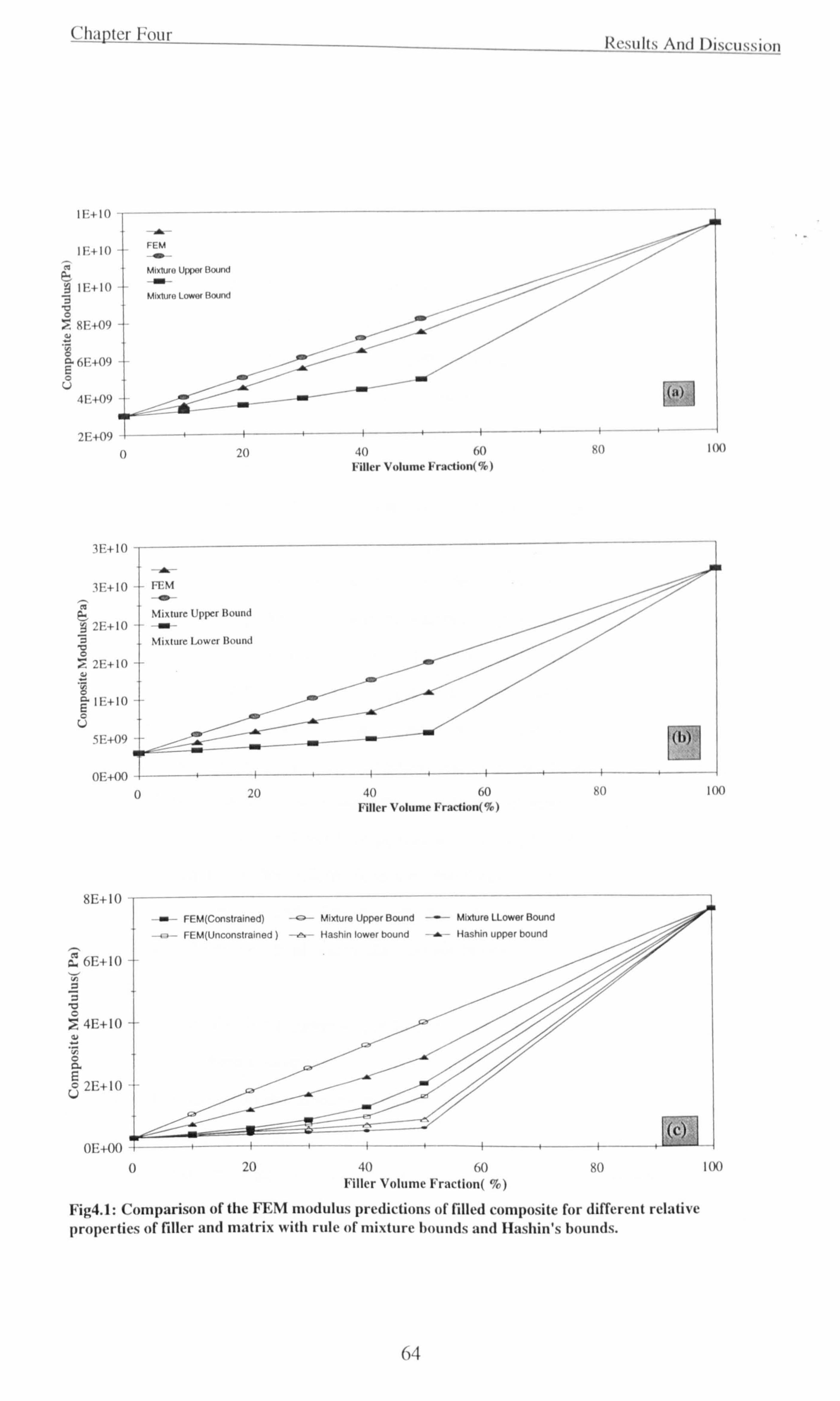
('hahtcr Four
IE+IOI- -- ý-
IF, +10
IE+IO
0 RE+09
a 6E+09 E 0
U
2G+09
0
FEM
Mixtur© Upper Bound
Mixture Lower Bound
1/
4
20 40 60 Filler Volume Fraction(9b)
40 60 Filler Volume Fraction(%)
3E+10
3E+10 FEM
Mixture Upper Bound 2F, +10 - --
,a Mixture Lower Bound
0 2E+10
E IE+10 0
U
5E+09
0E+00 A- '--T 0 20
8E+I0
6E+ 10
0
b 4E+I0
N 0
2E+I0
0E+00 0
-af FEM(Constrained) -2- Mixture Upper Bound Mixture LLower Bound
-<_ý - FEM(Unconstrained) -- Hashin lower bound -- Hashin upper bound
20 4(l 60 Filler Volume Fraction( %)
kC. tillll. l And I )isru. ý. tiiýni
SO
90
Fig4.1: Comparison of the FEM modulus predictions of filled composite for different relative properties of filler and matrix with rule of mixture bounds and Hashin's bounds.
100
100
1 (x)
64
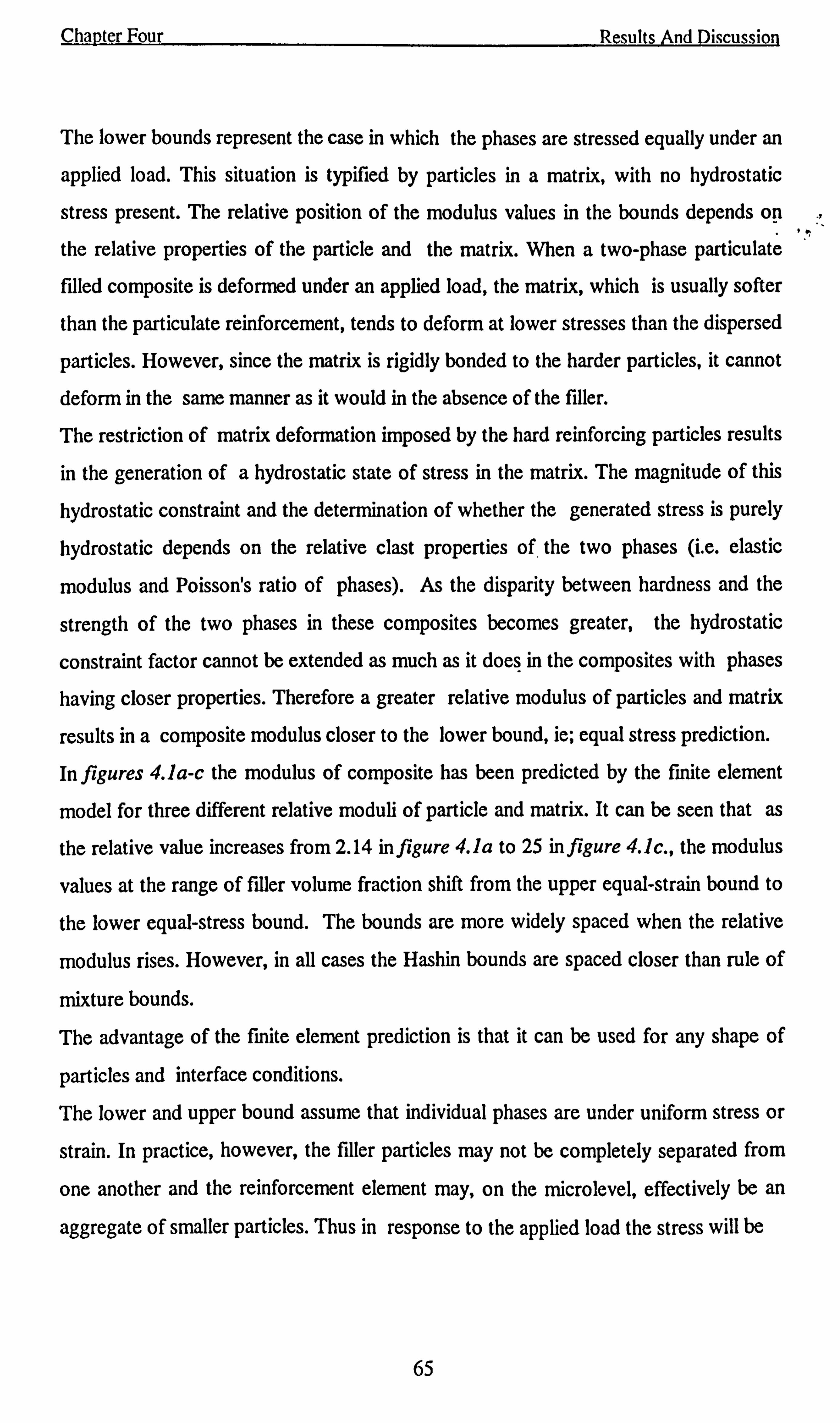
Chapter Four Results And Discussion
The lower bounds represent the case in which the phases are stressed equally under an
applied load. This situation is typified by particles in a matrix, with no hydrostatic
stress present. The relative position of the modulus values in the bounds depends on
the relative properties of the particle and the matrix. When a two-phase particulate
filled composite is deformed under an applied load, the matrix, which is usually softer
than the particulate reinforcement, tends to deform at lower stresses than the dispersed
particles. However, since the matrix is rigidly bonded to the harder particles, it cannot
deform in the same manner as it would in the absence of the filler.
The restriction of matrix deformation imposed by the hard reinforcing particles results
in the generation of a hydrostatic state of stress in the matrix. The magnitude of this
hydrostatic constraint and the determination of whether the generated stress is purely
hydrostatic depends on the relative clast properties of the two phases (i. e. elastic
modulus and Poisson's ratio of phases). As the disparity between hardness and the
strength of the two phases in these composites becomes greater, the hydrostatic
constraint factor cannot be extended as much as it does in the composites with phases
having closer properties. Therefore a greater relative modulus of particles and matrix
results in a composite modulus closer to the lower bound, ie; equal stress prediction.
In figures 4.1 a-c the modulus of composite has been predicted by the finite element
model for three different relative moduli of particle and matrix. It can be seen that as
the relative value increases from 2.14 in figure 4.1 a to 25 in figure 4.1 c., the modulus
values at the range of filler volume fraction shift from the upper equal-strain bound to
the lower equal-stress bound. The bounds are more widely spaced when the relative
modulus rises. However, in all cases the Hashin bounds are spaced closer than rule of
mixture bounds.
The advantage of the finite element prediction is that it can be used for any shape of
particles and interface conditions.
The lower and upper bound assume that individual phases are under uniform stress or
strain. In practice, however, the filler particles may not be completely separated from
one another and the reinforcement element may, on the microlevel, effectively be an
aggregate of smaller particles. Thus in response to the applied load the stress will be
65
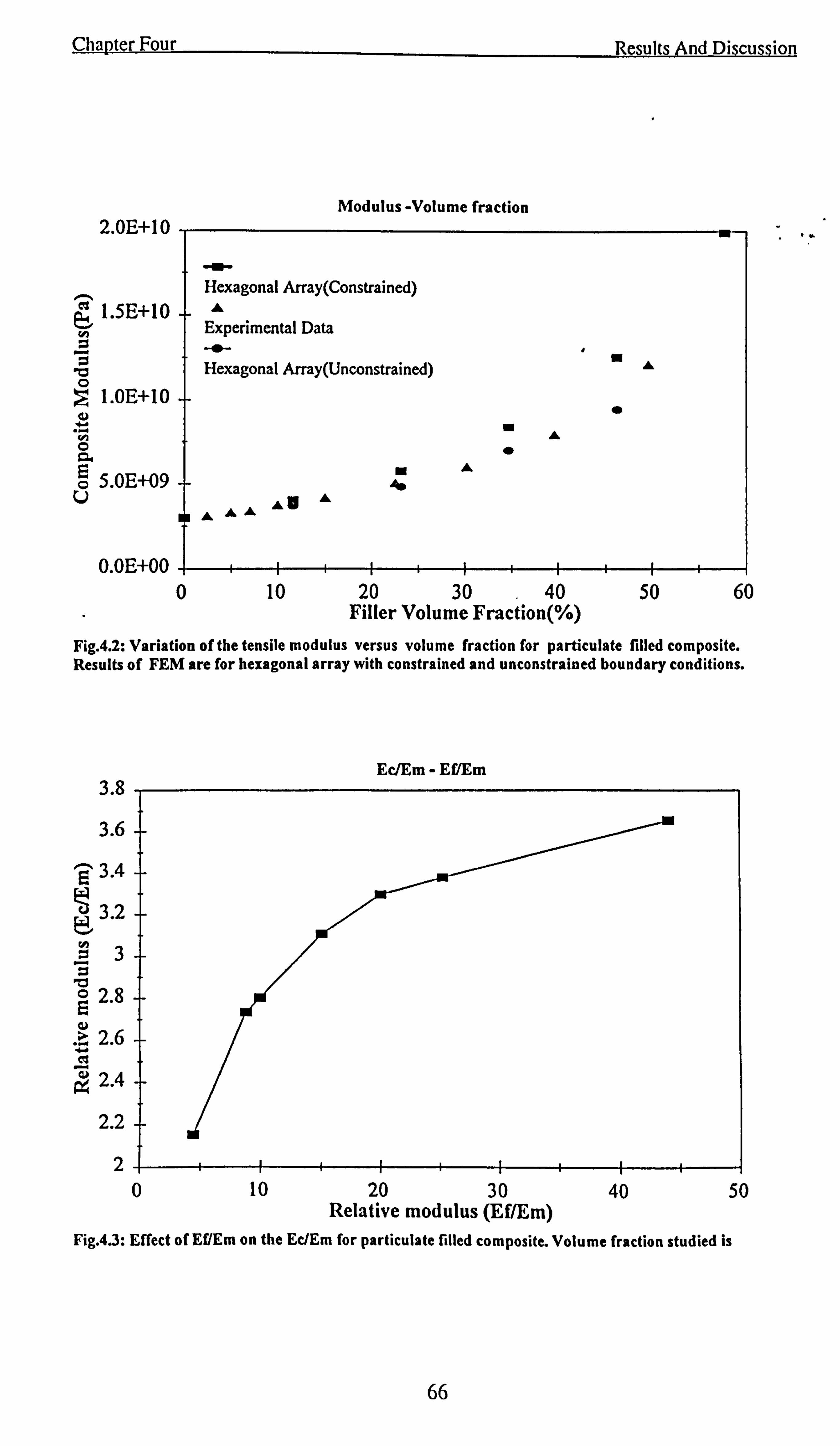
Chapter Four
2.0E+10
ý1.5E+10ý- ý ý ^. PC 0 :ý1.0E+10 Q ... ... 0 a
Modulus -Volume fraction
Hexagonal Array(Constrained) A
Experimental Data
Hexagonal Array(Unconstrained)
E S. OE+09 U
A, ýý ý0
A
m 0
A
4
Results And Discussion
m A
0
0.0E+00 -1ir-ý- E---F-º-r-ºri; 0 10 20 30 40 50 60
Filler Volume Fraction(%)
Fig. 4.2: Variation of the tensile modulus versus volume fraction for particulate filled composite. Results of FEM are for hexagonal array with constrained and unconstrained boundary conditions.
3.8
3.6
E 3.4
3.2
3
Ici 2.8
ez 2.6 w
2.4
2.2
2
0 ý ý
Ec/Em - Ef/Em
20 30 10 Relative modulus (Ef/Em)
H- 40
i 50
Fig. 4.3: Effect of Ef/Em on the EdEm for particulate filled composite. Volume fraction studied is
66
Chapter Four Results And Discussion
distributed unevenly between the particles and aggregates and the assumption of either
uniform stress or strain (uniform particle size and distribution) will be an over-
simplification.
4.1.2 Model predictions and experimental results
Accurately measured values of Young's modulus for epoxy resin reinforced with glass
spheres are available from literature. These experimental results agree well with our
finite element predictions as shown in figure 4.2. The differences can be attributed to
the assumptions that have been made in the model. The discrepancy between model
predictions and the experimental results may be due to ignoring the following factors
in the model.
4.1.2.1 Agglomeration
The filler particles may aggregate to form agglomerates much larger than the filler
particles. Agglomerates tend to contain voids and air filled spaces so that their
apparent volume is considerably greater than the true volume of the filler material.
If the agglomerates are hard and have appreciable mechanical strength, they will not
easily be broken and considering the weight of material added as filler, the filled
material can have a modulus greater than expected. Because the volume of the
aggregates in this case is larger than the true volume of the filler particles. Soft and
easily disintegrating aggregates, on the other hand, would be expected to give rise to
an opposite effect. The agglomeration of particles have a considerable effect at higher
volume fractions of filler and therefore this factor become more significant at higher
volume fractions.
4.1.2.2 Dewetting
At high concentration of fillers, all the individual particles might not be wetted by
matrix phase resulting in a poorer dispersion of the filler within the composite.
Instead, the particles tend to aggregate. Dewetting and poor dispersion are amongst
67
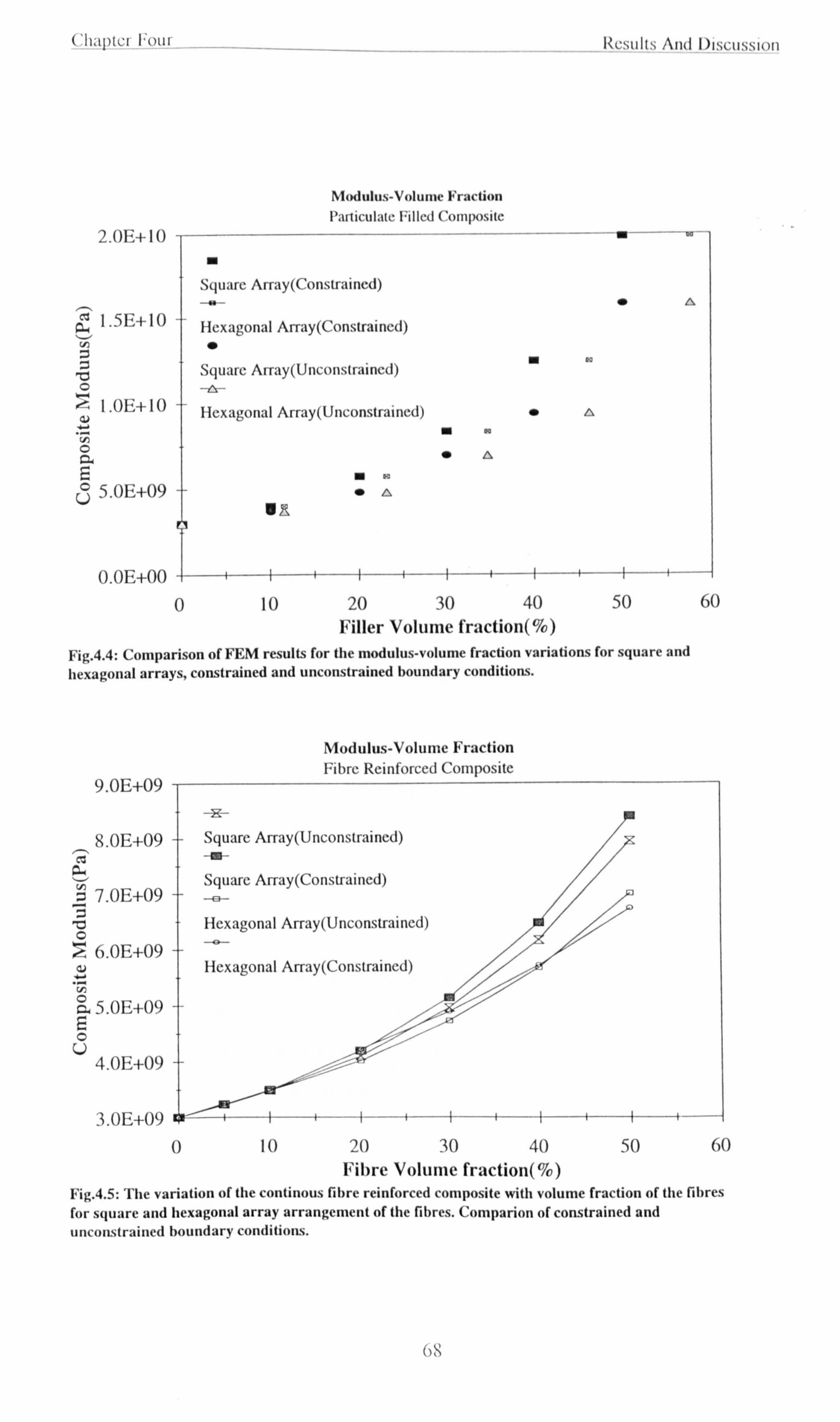
('Imhtcr Foui
2.0E+10 -,
, -. ä 1.5E+10 ý
(ID
v O
1.0E+10
5.0E+09 j
O. 0E+00 4 0
0
Modulus-Volume Fraction Particulate Filled Comlmsite
Square Array(Constraincd)
Hexagonal Array(Constrained)
Square Array(Uncons(raincd)
-a-
.ý
LIN Hexagonal Array(Unconstraincd) 40
V'R
.ý "o
.ý 0A
Itcsults And Discussion
0n
10 20 30 40 50 60 Filler Volume fraction(%)
Fig. 4.4: Comparison of FEM results for the modulus-volume fraction variations for square and hexagonal arrays, constrained and unconstrained boundary conditions.
Modulus-Volume Fraction Fibre Reinforced Composite
9.0E+09
8.0E+09 ý Squarc Array(Unconstraincd)
Square Array(Constrained) 7.0E+09
Hexagonal Array(Unconstrained)
6.0E+09 Hexagonal Array(Constraincd)
ý ý 5.0E+09
0 U 4.0E+09 -{-
3.0E+09 W' -'i 0 10 20 30 40 50 60
Fibre Volume fraction(%) Fig. 4.5: The variation of the continous fibre reinforced composite with volume fraction of the fibres for square and hexagonal array arrangement of the fibres. Comparion of constrained and unconstrained boundary conditions.
68
Chapter Four Results And Discussion
the reasons that make the production of composites with very high filler volume fractions impractical.
4.1.2.3 Adhesion and bonding
In theoretical analysis of the behaviour of the composites it is generally assumed that
the adhesion between the filler and the polymer matrix is perfect. By perfect adhesion it
is meant that there is no relative movement of the phases across the interface under the
applied loads. At higher applied stresses, however, the interfacial bond may break, and
the adhesion is no longer perfect. Thus, the magnitude of the applied stresses often
determines whether there is a perfect adhesion or not. In reality, the degree of
adhesion does not appear to be an important factor as long as the frictional forces
between the phases are not exceeded by the applied stress. In most filled systems there
is a mismatch between thermal expansion coefficients of the phases which results in a
mechanical bond due to thermally induced stresses.
In many practical cases it cannot be assumed that there is a perfect adhesion between
the filler and the matrix. In extreme cases of debonded particles it can be assumed that
the particles act as holes and, therefore can seriously decrease the composite modulus
with increasing filler content. It can be argued that the unbonded particles do not act
entirely as holes, since they also restrain the matrix from collapsing.
If the bond or adhesion between filler and polymer is weak, the bond may break when
a load is applied. The polymer will then deform more than the filler so that
unsymmetrical cavities and voids develop around each filler particle.
A change of the matrix-filler adhesion has a smaller effect on composite modulus than
its strength. The latter is much more dependent on the pre-treatment of the filler
surface. Thus the filler is less efficient as a reinforcing agent, and in extreme cases the
modulus of the composite can be reduced rather than being increased by the addition
of filler.
4.1.2.4 Arrangement
In practice the arrangement of the filler particles in a composite can never be uniform
and the interparticle spacing varies in different parts of the composite. It has been
69
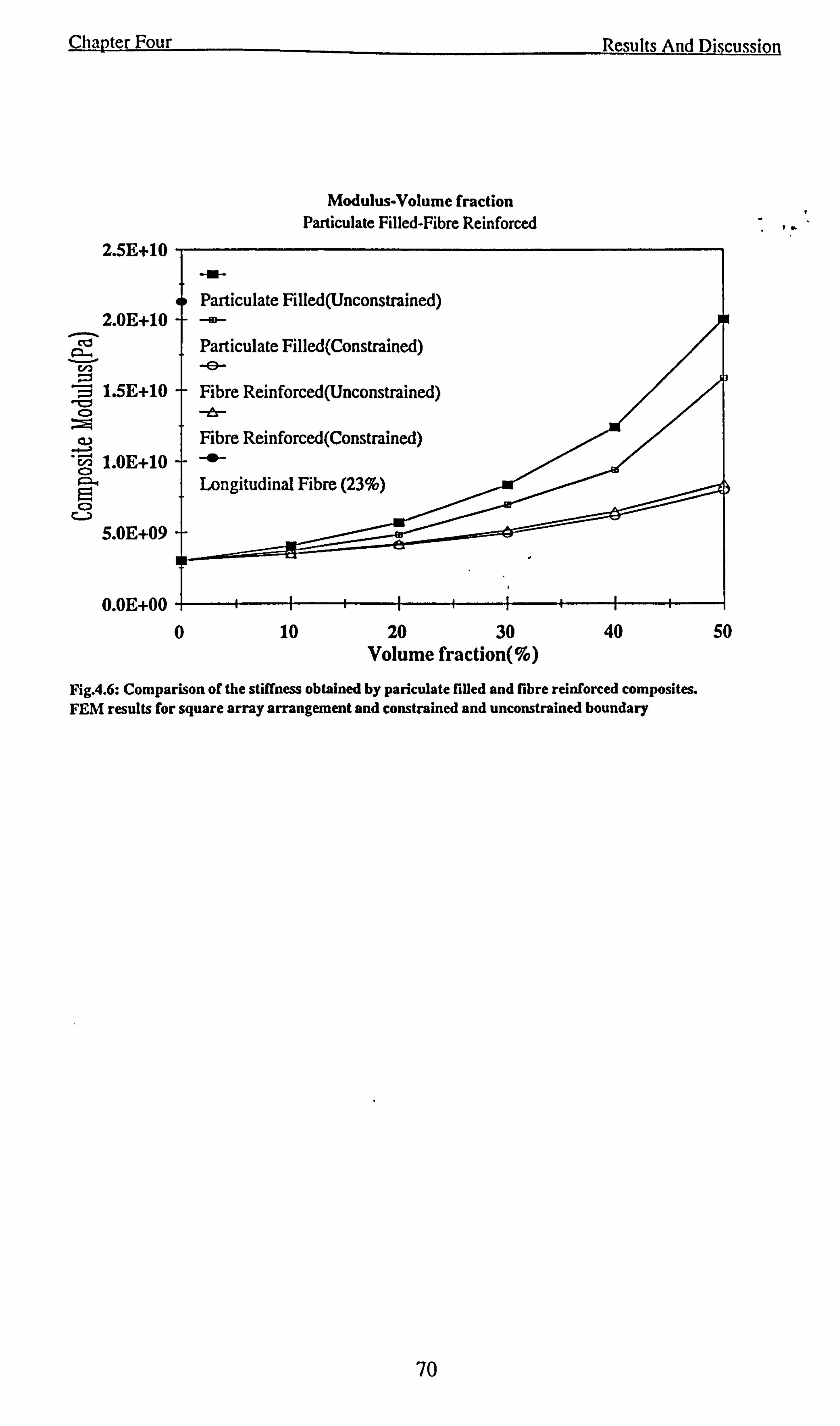
Chapter Four
Modulus-Volume fraction Particulate Filled-Fibre Reinforced
Results And Discussion
2.5E+10 -i
ý co
G1.
2.0E+10
-m-
ý U)
1.5E+10
I Particulate Filled(Unconstrained) -ED- Particulate Filled(Constrained) -e- Fibre Reinforced(Unconstrained)
-A- Fibre Reinforced(Constrained)
ö 1.0E+10 -I- I=L4 E 0
S. OE+09 I
0.0E+00 -F 0
-a- Longitudinal Fibre (23%)
q -1- 10 20 30
Volume fraction(%)
i -+ 40
ý
Fig. 4.6: Comparison of the stiffness obtained by pariculate filled and fibre reinforced composites. FEM results for square array arrangement and constrained and unconstrained boundary
50
70
Chapter Four Results And Discussion
shown that when particles are distributed randomly, a lower composite modulus is
obtained. A combination of finite element modelling and spatial statistical techniques
has been used in the simulation of composites with randomly distributed filler
particles.
In this project two different types of particle arrangements in the form of square and
hexagonal arrays are examined to show the effect of the particle distribution on the
final physical properties of the composite. The results are shown in figure 4.4 for a
particulate filled composite. The same comparison of the effect of the arrangement of
reinforcing phase can be seen in figure 4.5 for a fibre reinforced composite. In both
cases the hexagonal array gives lower composite modulus for the same filler volume
fraction and the hexagonal array gives a higher volume fraction for the same particle
spacing. The hexagonal array can be considered to be a more random arrangement
compared to the square array.
4.1.2.5 Filler particle shape
In our model we assume that the particles are spherical and of the same size.
Practically the filler particles are not uniform in size and only a few fillers are
spherical in shape. However, since most particles have nearly the same dimensions
in all directions, they can be approximated by sphere. Deviations of experimental
results from the model may be caused by more important factors than small
deviations of the particles from spherical shapes.
Despite the described simplifying assumptions our model predictions compare closely
with the experimental results. The agreement between model predictions and
experimental results is more obvious when unconstrained boundary conditions is
imposed and hexagonal packing is chosen to show the distribution of the particles.
It can be shown that the addition of particles produces a substantial increase in
composite modulus. However, asfigure 4.3 indicates the effect of increase in particle
modulus gradually diminishes becoming asymptotic to the modulus of an infinitely
rigid particle.
71
Chanter Four Results And Discussion
4.2.3 Boundary conditions used in the finite element model
The conditions at the boundary of the cell which is perpendicular to the boundary
under tensile load can affect the result of the analysis. When boundary conditions with '.
constraint are imposed, for each point of the modulus-volume fraction curve we need
to follow two steps of loading. The results of these steps are superimposed and the
total and final point is calculated. Under this set of boundary conditions we enforce
geometric compatibility and therefore the outer sidewall of the cell remains straight. When the unconstrained boundary conditions is employed, every point along the
sidewall is stress free. However, since the constraints are released, the sidewalls do not
remain straight. The results obtained for these sets of boundary conditions are
compared for both particulate and fibre reinforced composites and are shown in figure
4.6. The results predicted using unconstrained boundary condition are lower than the
results found for the constrained boundary conditions.
72
Chapter Four Results And Discussion
4.2 COMPOSITES FILLED WITH RIGID PARTICLES
In this section the response of epoxy resin filled with glass particles to tensile and
compressive loading is studied. The physical properties of the epoxy resin and glass
filler used as the input values for the finite element program are presented in table 4.1.
4.2.1 Young's modulus
The predicted values of the Young's modulus for composites filled with hard particles
are compared with experimental data in figure 4.4. The theoretical models which are
used to explain the variations of the modulus of polymer composites with volume
fraction do not normally include the effect of filler particle size. However, experimental
observations of Spanoudakis and Young (Spanöudakis and Young, 1984) show that
there is a clear reduction in the modulus of a composite with increasing particle size for
a given volume fraction of particles.
Relatively low values of Young's modulus for large particle sizes have been attributed
to the "skin" effect. Lewis and Neilsen suggested that in the moduli measurements,
the properties of the surface are emphasised at the expense of the interior of the
composite. This leads to a higher error for larger particles where the surface "skin" is
depleted of particles. This could explain the drop in modulus with increasing particle
size. The error due to "skin" effect can be removed by the extrapolation of measured
values for particles with zero size (i. e. points).
4.2.2 Stress distribution
4.2.2.1 Concentration of direct stress
The maximum direct stress concentration which is the maximum principle stress is
found to be in the resin above the pole of the sphere. The precise position and value of
the maximum stress concentration of the applied stress vary with the volume fraction
of the filler. The magnitude of the stress concentration of applied stress increases with
volume fraction of added glass particles which is due to increasing interactions
73
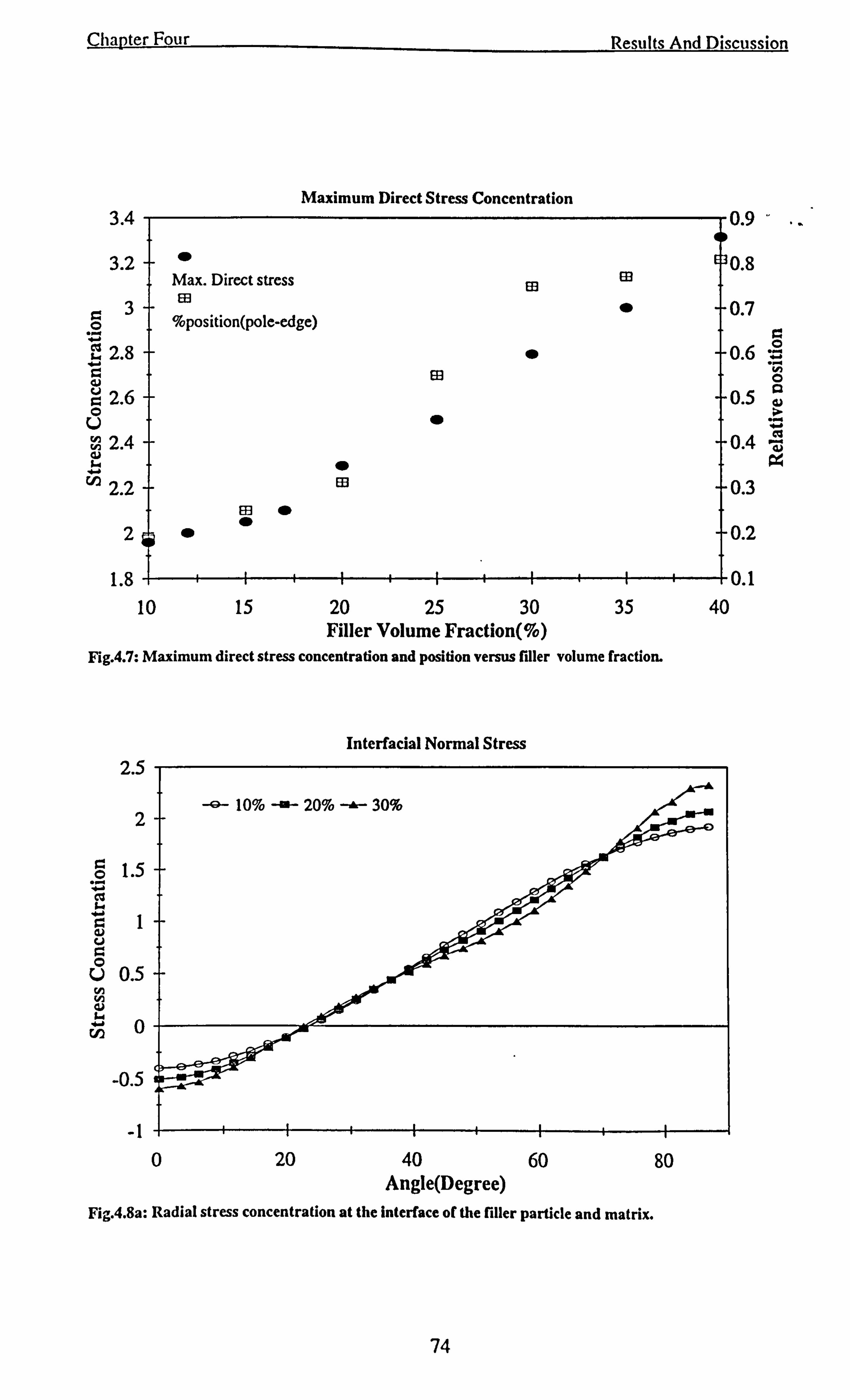
Chapter Four
3.4
3.2
3 0 ... .ý 2.8
ý 2.6 0 U
2.4 ý ... `'o 2.2
Maximum Direct Stress Concentration
" Max. Direct stress
%position(pole-edge)
EB
0
E13 "
40 ED
03
0
Results And Discussion
0.9
0.8 EB
0 0.7
0.6 ... h O
0.5 .ý
0.4
0.3
24 "- t0.2 T
1.8 +-I-+-ý-+- Iii0.1 10 15 20 25 30 35 40
Filler Volume Fraction(%) Fig. 4.7: Maximum direct stress concentration and position versus filler volume fraction.
2.5
-1 ý 0
4 -}- 20
Interfacial Normal Stress
i ý-
40 60 80 Angle(Degree)
Fig. 4.8a: Radial stress concentration at the interface of the filler particle and matrix.
74
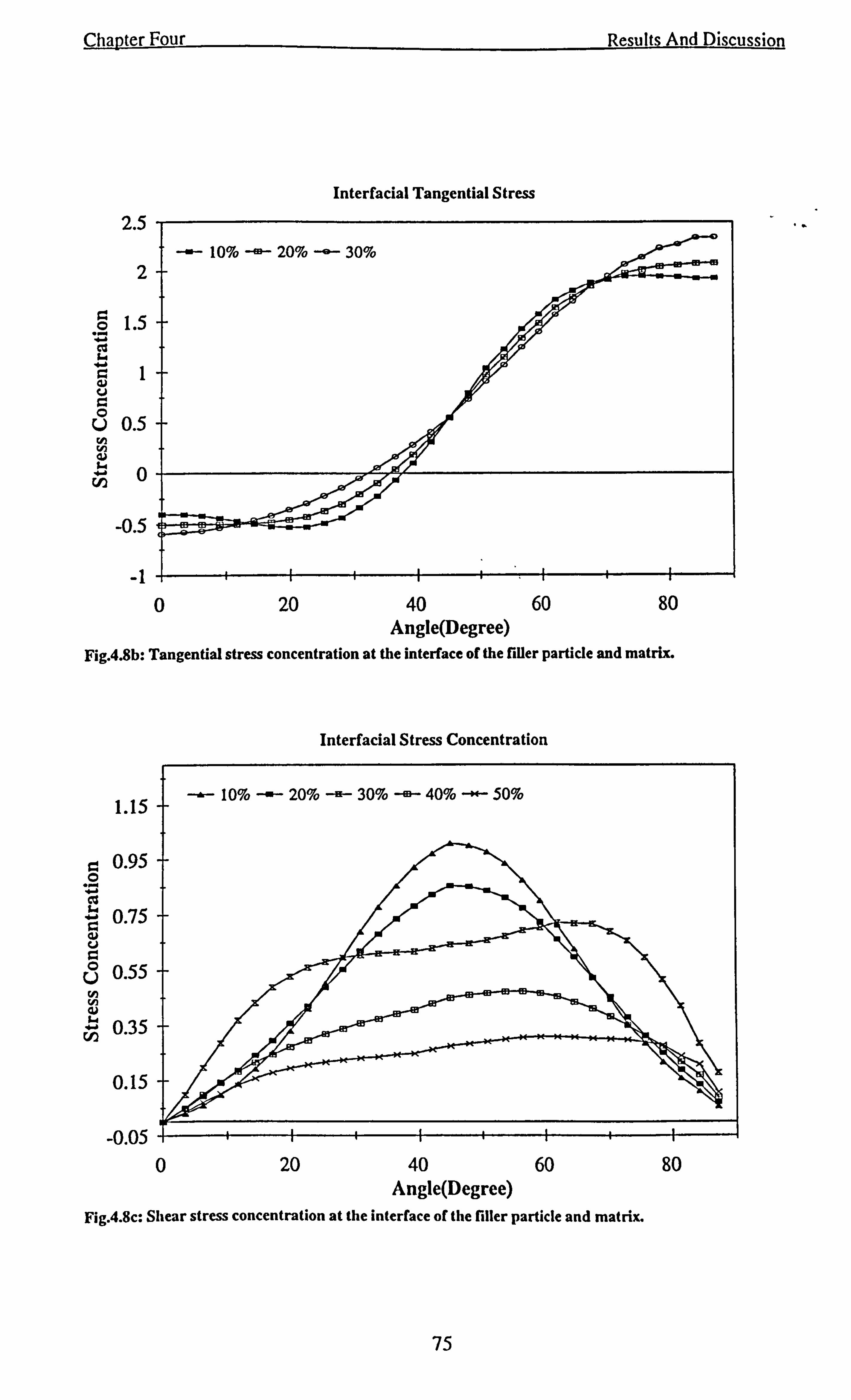
Chapter Four
2.5
-1 ý 0 20
Results And Discussion
Interfacial Tangential Stress
40 60 Angle(Degree)
80
Fig. 4.8b: Tangential stress concentration at the interface of the filler particle and matrix.
Interfacial Stress Concentration
0 20 40 Angle(Degree)
60
Fig. 4.8c: Shear stress concentration at the interface of the filler particle and matrix.
75
80
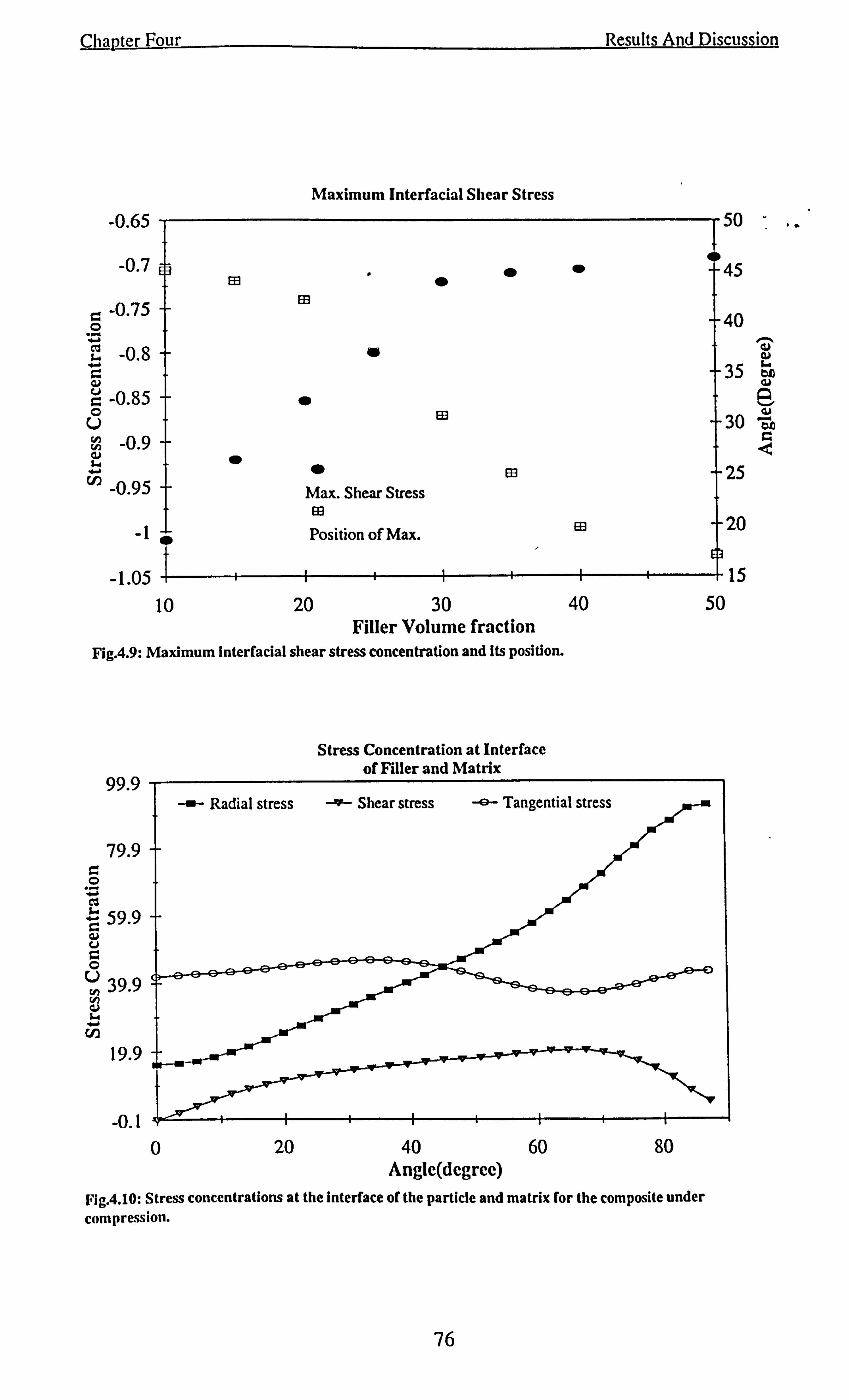
Chapter Four Results And Discussion
Maximum Interfacial Shear Stress
-0.65
-0.7
-0.75 0 *Z sý -0.8 i- 4ý
"" ®"
a ý -0.85 " 0 U
-0.9
a
ES
50 . t45
+40 aý v
35 cn ý
30 ö0 ý ý
0® 25 to -0.95 Max. Shear Stress
83 --
-1 Position of Max. ® 20 410
-1.05 15
10 20 30 40 50 Filler Volume fraction
Fig. 4.9: Maximum Interfacial shear stress concentration and Its position.
Stress Concentration at Interface of Filler and Matrix
99.9
79.9
cn
20 40 Angle(degree)
60 80
it' ig. 4.10: Stress concentrations at the interface of the particle and matrix for the composite under compression.
-"- Radial stress -'9- Shear stress -e- Tangential stress
76
Chapter Four Results And Discussion
between the stress fields around the filler particles as their separation decreases.
Stress concentration in this work is defined as the stress value normalised by the stress
applied to the composite and the relative position is the distance from the pole
normalised by the pole-edge distance.
The position of maximum stress concentration factor of the applied stress varies in the
studied cases. This is shown in figure 4.7. At high filler volume fractions the position
is at the edge of the grid, which is the midway between the particles. At lower volume
fractions the position is relatively closer to the particle in the cylinder under analysis,
which is further away from its adjacent particles. Taking into account that the distances
between adjacent particles for different volume fractions is variable, the maximum
distance between the position of stress concentration and adjacent particle was
calculated. This distance decreases rapidly with increasing filler volume fraction.
4.2.2.2 Stresses at the interface
Stresses around the interface are transformed to polar coordinates. Radial and shear
stresses on either side of the interface, in the glass and resin are identical. It is found
that the stress transferred to the glass sphere is substantial. This leads to a sharp
increase in the stiffness with increasing volume fraction of particles.
As figure 4.8a shows the maximum radial stress is at the pole of the particle sphere
for all volume fractions. The variations of the value of this stress concentration with
filler volume fraction is similar to that of the maximum stress concentration. Radial
stress is tensile at the pole and compressive at the equator for a spherical particle. At
position 0= 22° the stress is zero for all volume fractions. The variation of the
tangential stress in the matrix at the interface is shown in figure 4.8b.
There is a maximum in radial-tangential shear stress as it can be seen in figure 4.8c.
Both the value and the position of this stress concentration vary with volume fraction.
The absolute value of the stress concentration factor decreases with increasing volume
fraction. This decrease is explained by considering the source of this stress
concentration, which is the difference between the moduli of the particle and its
surrounding material. As the volume fraction of spheres increases this difference
decreases, and hence the rate of this decrease becomes significantly (- 4 times) smaller
77
Chapter Four Results And Discussion
than the rate of the increase of the concentration of applied stress. Figure 4.9 indicates
that at higher volume fractions the site of this maximum concentration of shear stress
moves closer to the pole of the sphere.
Stresses around the interfaces of spherical particles have previously been considered by
Dekkers and Heikens ( Dekkers and Heikens, 1983). For a poorly bonded interface
they postulate that a crack will form around the interface because of the tensile radial
stress. Using the constituent material properties very close to those we have used,
they predicted that the interfacial crack should grow up to an angle of 0= 68° to 70°,
depending on the remaining friction of the debonded interface. The magnitude of the
radial stress concentration at the pole is not much smaller than the maximum
concentration of the applied stress. Therefore for the tensile loading, debonding from
the pole is expected. Under tensile applied stress the radial stress at the equator is
compressive.
4.2.3 Compression
The radial stress would be tensile at the equator of the particle interface if the applied
stress is compressive. Figure 4.10 shows the distribution of the stresses at the particle
and matrix interface. Although the absolute value of this stress at the equator is almost
an order of magnitude smaller than its value at the pole it may however be sufficient to
cause debonding from the equator of the sphere under the condition of the applied
compression.
4.2.4 Concentration of yield stress
The contour diagrams of the Von Mises stress, direct stress and shear stress
concentrations are shown in figures 4.11a-c. In the contour diagram of the Von Mises
stress two positions where Von Mises stress reaches its maximum are found: the first
point is in the resin above the pole of the sphere in the close vicinity of the position of
the maximum direct stress concentration; the second point is near to the position of the
maximum shear stress at the interface. The values of these stress concentration factors
vary with volume fraction as is shown in figure 4.12. Their positions vary in the same
directions as the positions of the associated concentrations of the direct stresses.
Figure 4.13 shows that the magnitudes of the maximum concentrations of
78
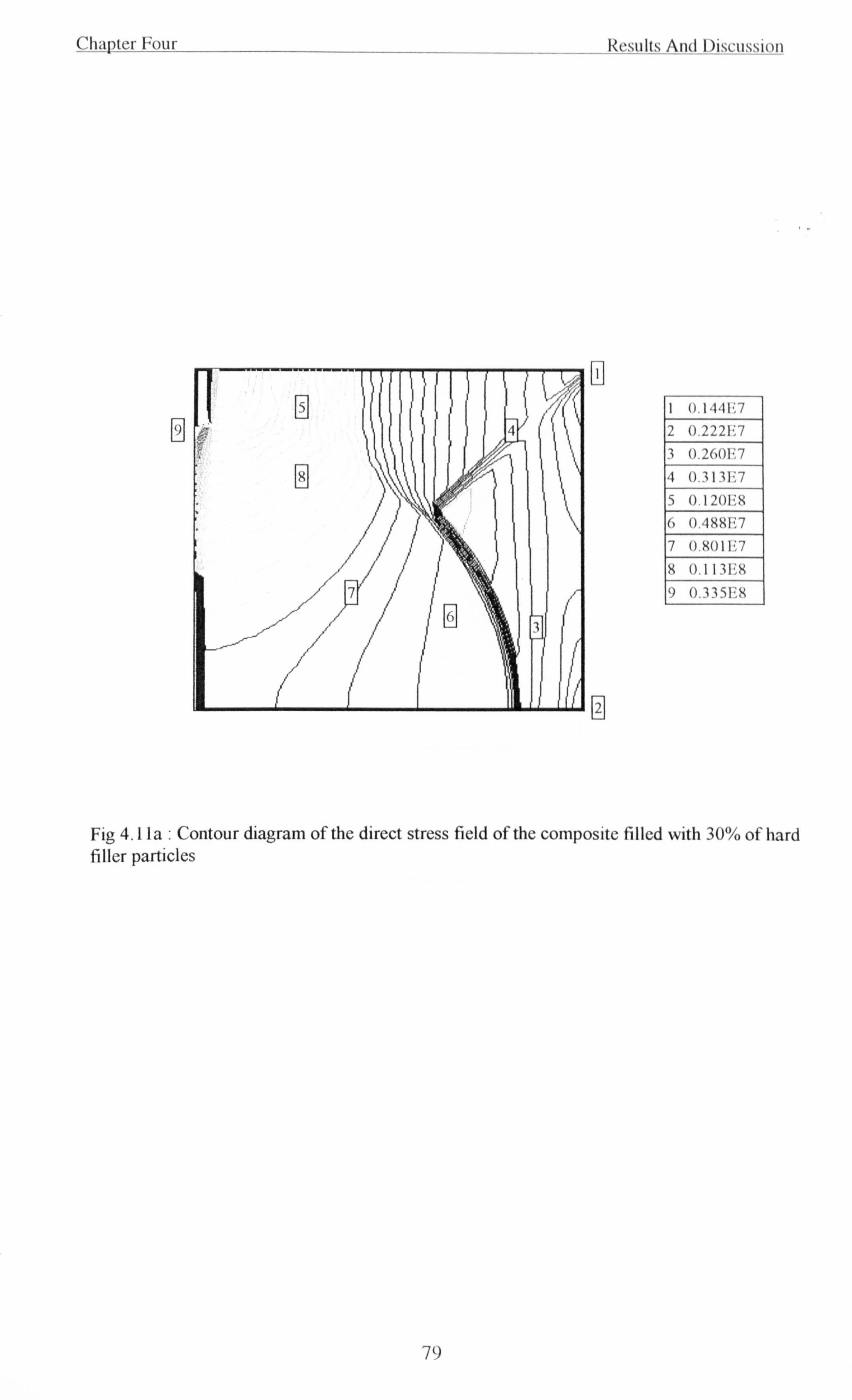
Chapter Four Results And Discussion
q
I
1 U. 1441? 7
2 0.2221? 7 3 (). 260F7
ý1 0.3131? 7 5 0.1201? R 6 1). 4RxF. 7 7 O. 8011{7
9 0.1 131? x 9 0.3351? x
0
Fig 4.1 la : Contour diagram of the direct stress field of the composite filled with 30% of hard filler particles
79
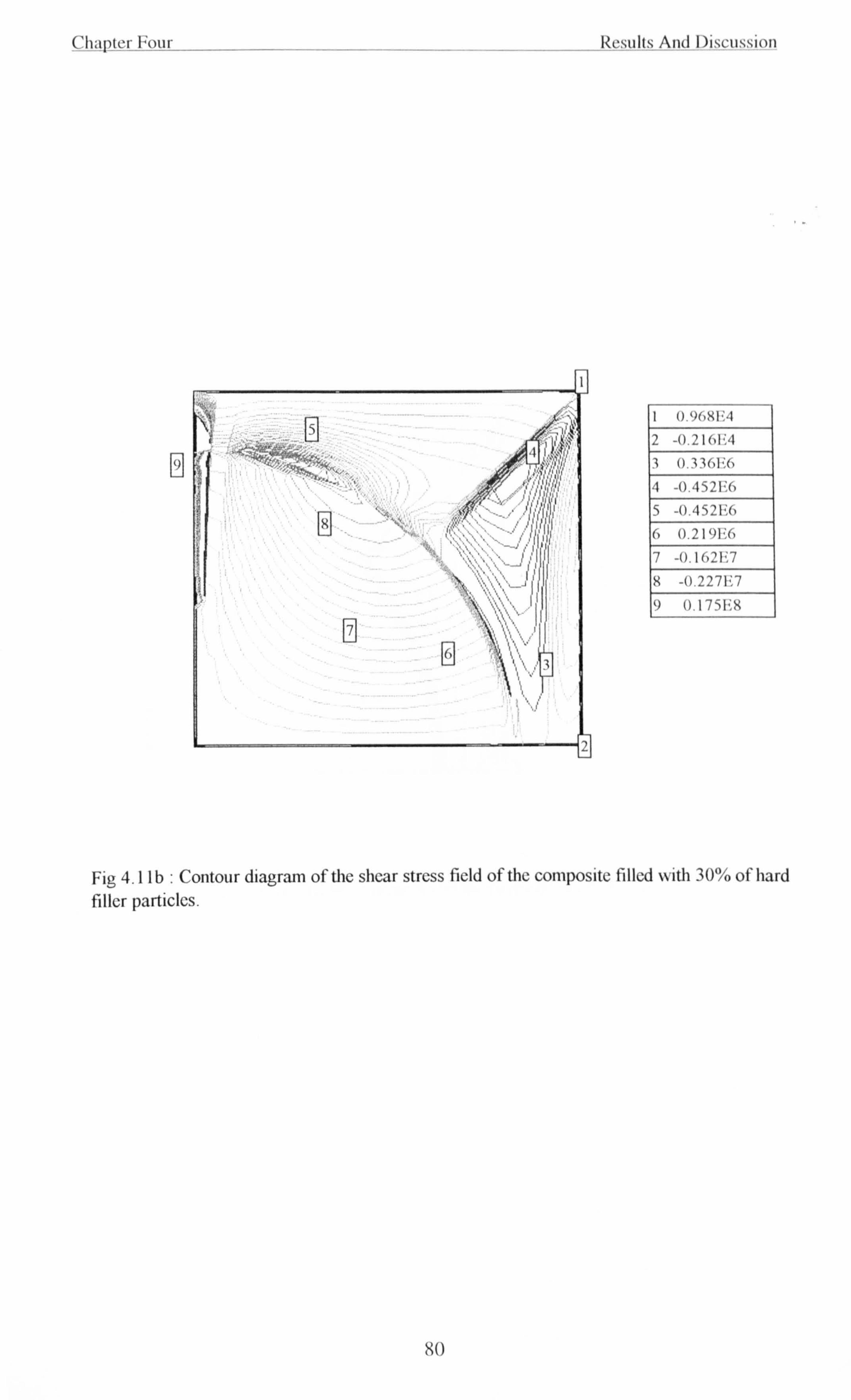
('h. ºhtcr J Four -
Results And Discussion
9 I, ý ', r !
I U. 9C, K1'A
2 -O. 21h1? 4 3 U. 33(, l{0
4 -0.452F6
R r;
5 -0.452F6 6 0.2191? 6
7 -0.1621,17 9 -t). 227F7
0
I
G
9 0.175FR
Fig 4.1 1b: Contour diagram of the shear stress field of the composite filled with 30% of hard filler particles.
80
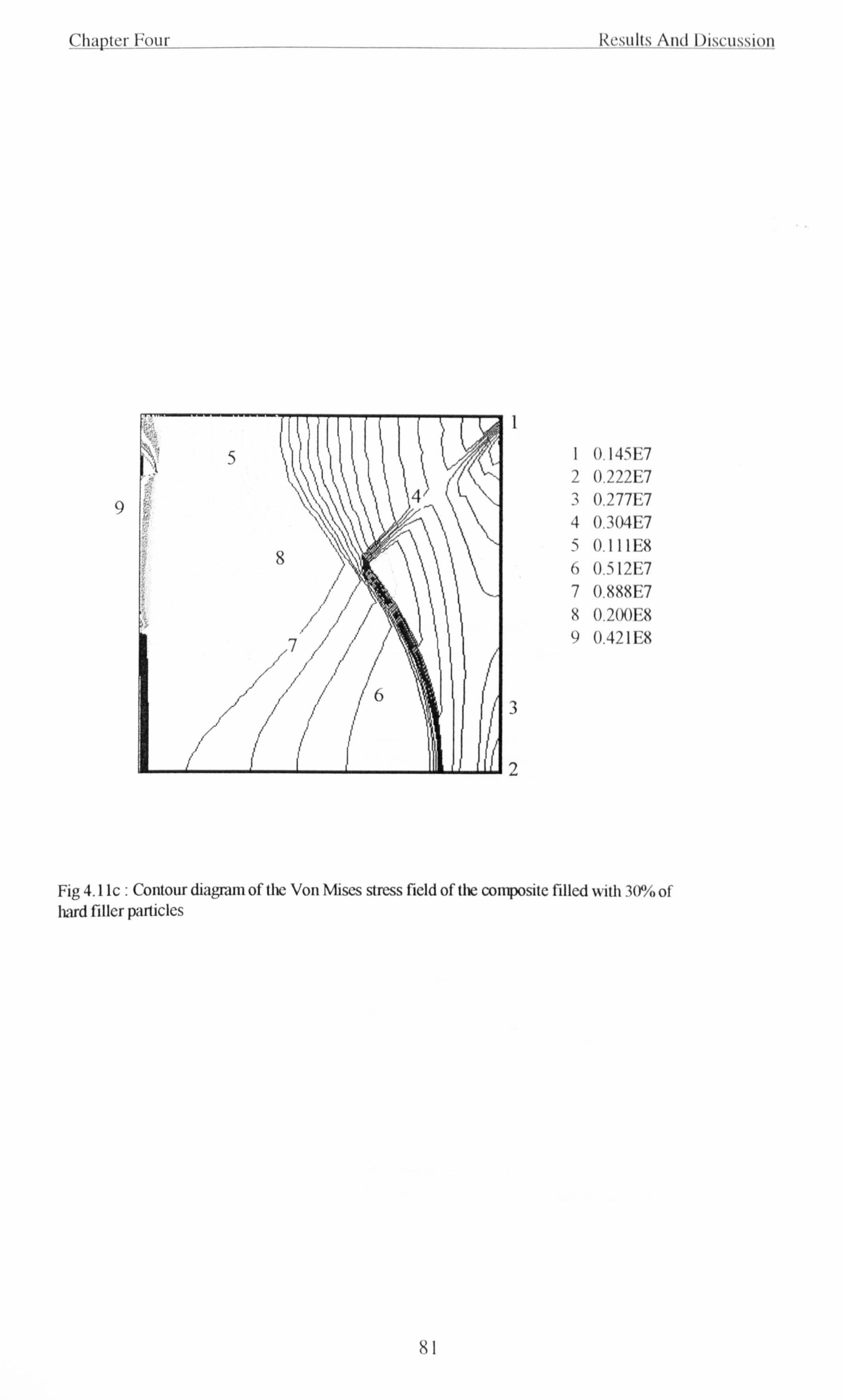
Chapter Four _
Ilrsults And I)iscussion
I 0.145E7 2 0.222E7 ý 0.277E7 4 0.3(>4E7 5 O. 1 1l ER 6 0.512E7 7 0.8RRE7
0.2(X)E8 ýý 0.421 Ex
Fig 4.11 c: Contour diagram of the Von Mises stress field of the composite filled with 3(YYo of hard filler particles
81
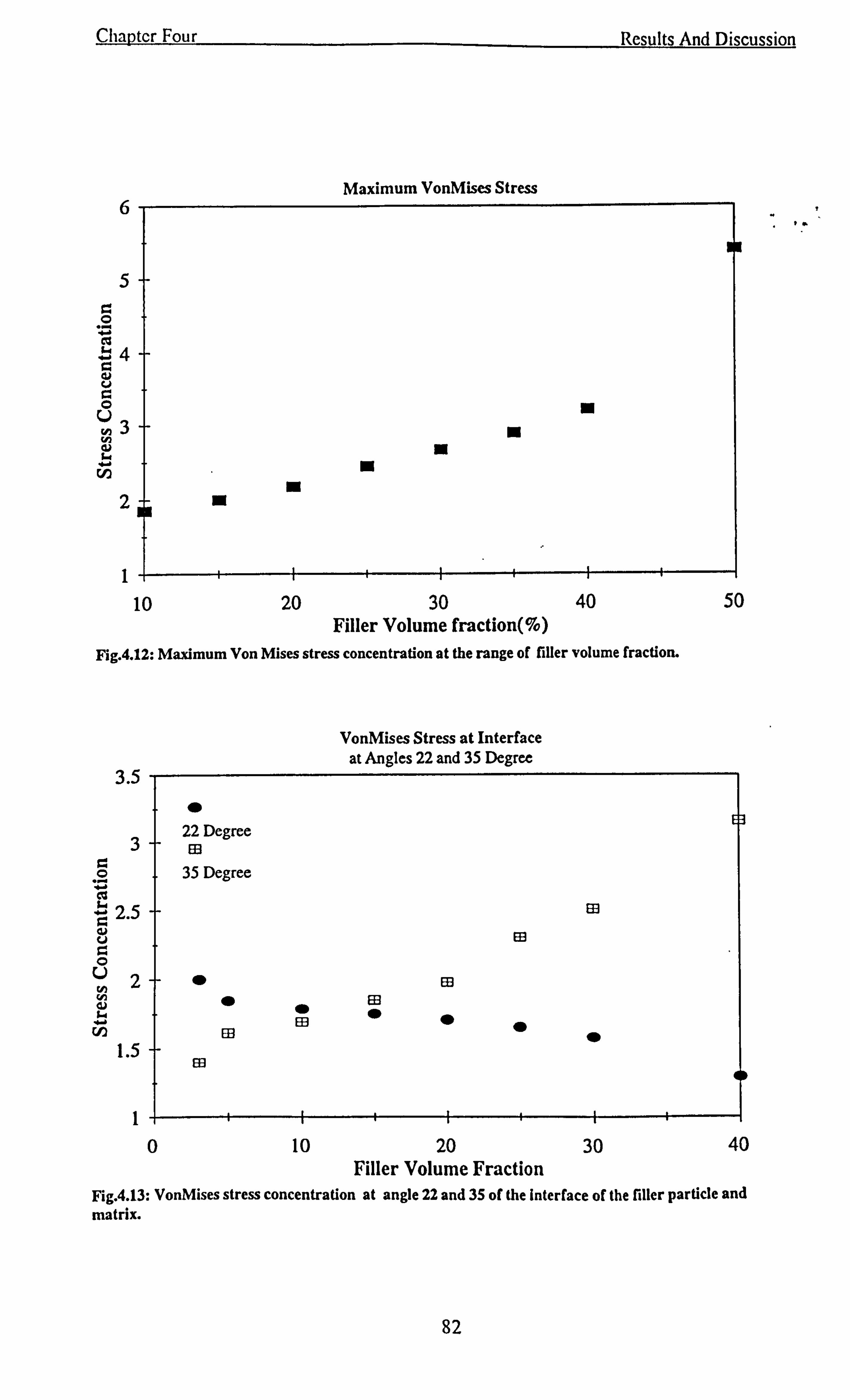
Chapter Four
6
5+ A 0 ... .ý ý ý `' 4 a ý, U A 0 c) 3 ý ý ý, w rn
2 A 1
3+
Maximum VonMises Stress
Results And Discussion
10 20 30 40 Filler Volume fraction(%)
Fig. 4.12: Maximum Von Mises stress concentration at the range of filler volume fraction.
VonMises Stress at Interface at Angles 22 and 35 Degree
3.5
ý 0 .... a w 2.5 ý u ý 0 U
m m
" 22 Degree
35 Degree
93
E13
9+" PR ý-- rA "® " w®""
1.5+ Ell
0 0
50
1 0 10 20 30 40
Filler Volume Fraction Fig. 4.13: VonMises stress concentration at angle 22 and 35 of the interface of the filler particle and matrix.
82
Chapter Four Results And Discussion
the Von Mises stress vary with volume fraction in the same way as the associated
stress concentrations, although the range of the variation of Von Mises stress is very
small. The stress peak located above the pole is greater at higher volume fractions of
the filler, but at volume fractions below about 15% the maximum located at the
interface is greater. Dekkers and Heikens (Dekkers and Heikens, 1983) studied the
shear band formation for very low volume fractions of glass beads in various polymer
matrices. They found shear band formation at the interface, at 0= 45°. The results of
our finite element analysis for similar composites are given in figure 4.14 which show
that at low volume fractions the maximum concentration of Von Mises stress is at the
interface, at 0= 40°.
The Von Mises stress at which yield occurs is dependent on the hydrostatic stress as
explained earlier in this chapter. The hydrostatic stress values corresponding to the
points of maximum Von Mises stress were calculated. Under the application of tensile
stress the hydrostatic stress is tensile. The hydrostatic stress concentration remains
almost constant up to around 20% volume fraction of filler, but it increases rapidly for
higher volume fractions. The maximum hydrostatic stress concentration occurs at the
pole of the particle.
4.2.5 Fracture behaviour
Crack growth is generally considered to move in the direction of the position of
maximum direct stress. Our model predicts that the position of maximum direct stress
is above the pole. These predictions correspond with the experimental observations
(Spanoudakis and Young, 1984).
For a well bonded sphere, at low volume fractions, crack growth is developed towards
the resin above the pole of the sphere. Smearing of resin around the pole of the sphere
is observed. This type of fracture appearance contrasts with the observed crack growth
in epoxy resin containing poorly bonded glass particles which is found to be attracted
to the equator of the sphere. The stress distribution in composite with poorly bonded
filler particle is similar to that of a composite containing holes. The site of the
maximum stress concentration is found to be at the equator of the sphere.
pw
83
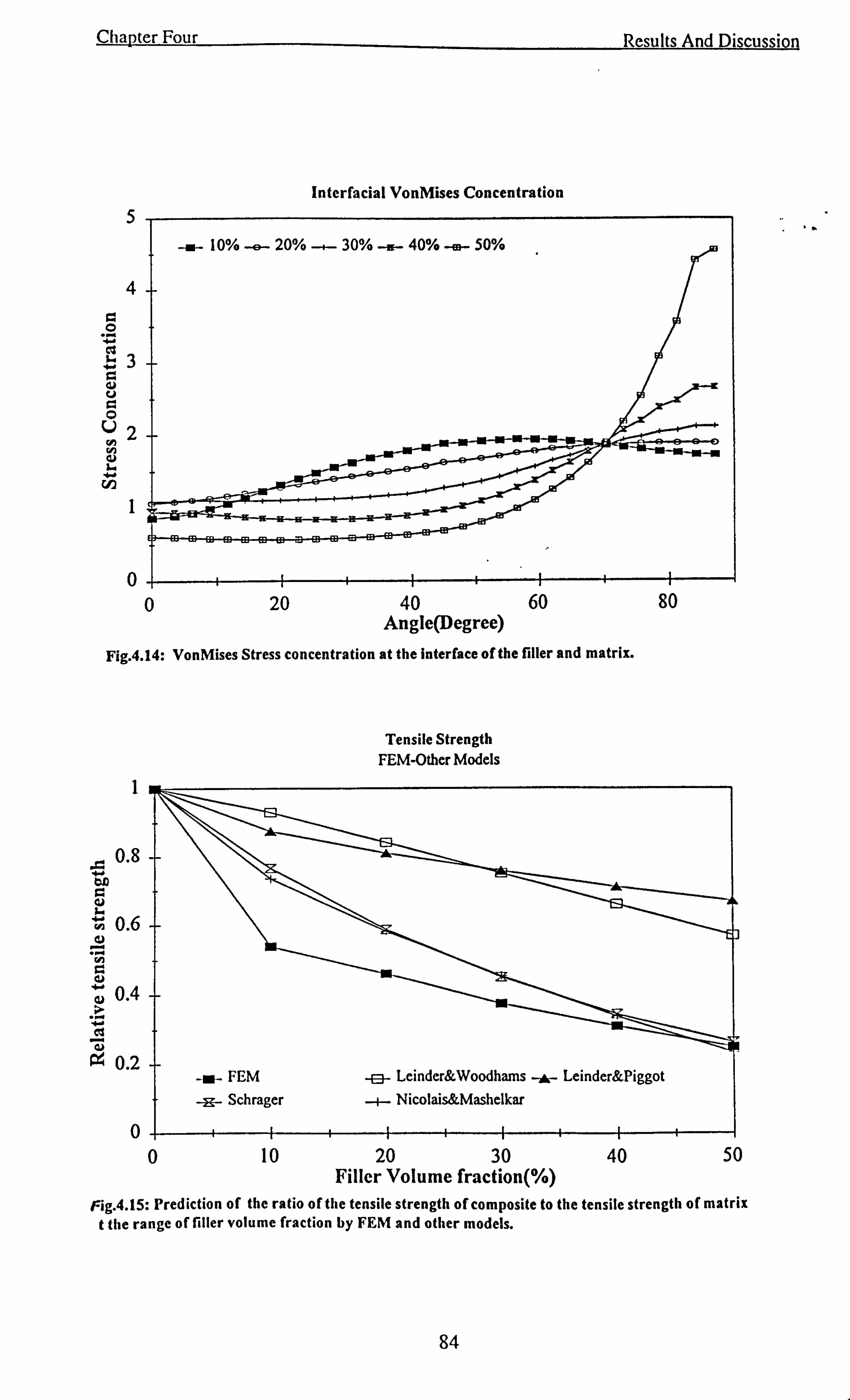
Chapter Four
0
Results And Discussion
Interfacial VonMises Concentration
r+ '+iii
20 40 60 80 Angle(Degree)
Fig. 4.14: VonMises Stress concentration at the interface of the filler and matrix.
Tensile Strength FEM-Other Models
-ý- FEM -e- Leinder&Woodhams -, &- Leinder&Piggot
ý- Schrager -4- Nicolais&Mashelkar
0 10 20 30 40 Filler Volume fraction(%)
50
Fig. 4.15: Prediction of the ratio of the tensile strength of composite to the tensile strength of matrix t the range of filler volume fraction by FEM and other models.
84
Chapter Four Results And Discussion
The amount of resin smearing around the pole of a well bonded sphere would be
dependent on the position of the crack with respect to the sphere. Our results show ,w
that at low volume fractions the maximum distance is much further away from the
sphere than for high volume fractions. Thus the model predicts that more smearing
would occur if there are no spheres visible in the fracture surface. Greater smearing at
low volume fractions has been observed. (Spanoudakis and Young, 1984)
It is found that besides matrix properties, strain rate and temperature, the degree of
interfacial adhesion has a profound effect on the competition between craze and shear
band formation. In cases where the beads adhesion are perfect craze formation is
favoured, whereas for poorly adhering beads shear band formation is dominant. This
effect is caused by the difference in local stress situation, craze formation becomes the
controlling factor under a triaxial stress state and shear band formation becomes the
dominant factor under a biaxial stress state. In the case of an excellently adhering glass
bead, the crazes form near the pole. Stress analysis shows that these are regions of
maximum dilatation and maximum principle stress. At a perfectly bonded glass bead
experimental observations show that the shear bands form near the surface of the bead
at 45° from the poles which are defined by the axis of symmetry maximum principal
shear stress and the density of maximum distortion energy. Our results confirm these
observations.
In the case of poor interfacial adhesion between glass beads and matrix, both craze and
shear band are preceded by dewetting along the interface between bead and matrix. At
dewetting a curvilinear interfacial crack is formed, starting at the pole and propagating
in the direction of the equator until, at an angle of about 60° from the pole, a craze or
shear band originates at the tip of the interfacial crack.
Neilsen suggested a very simple model based on the assumption of Hookean behaviour
up to breaking strains. In this case the following relation can be written:
Q, = EE, (4.3)
85
Chapter Four Results And Discussion
where E is the tensile modulus and c is the elongation at breaking point, and c may be
expressed as:
Ec=Em(1-V f 1/3
) (4.4)
where c,,, is the elongation at the breaking point of the matrix. Using the above
relations the relative strength of the composite is found as:
Eý v3 ßnr=-(1-V )
Em f (4.5)
The ratio Ec/Em can be calculated by the finite element model.
There are other theoretical models which predict the strength of the filled composites
and a few of them are brought to attention for comparison with the results of our finite
element model. The constants in the following models are given for the glass filled
epoxy composite.
1. Leidner and Woodham (Leidner and Woodham, 1978):
Qc=0.83paVf+Kam(1-Vf)
where pa=1540 psi, K=0.8 or 0.9.
2. Piggot and Leidner (Piggot and Leidner, 1974):
6c=am(1-0.5Vj6)
3. Nicolais and Mashelkar (Nicolais and Mashelkar, 1976):
(4.6)
(4.7)
Q, =6m-f%Vb (4.8)
with b=1.21 and n=0.66
86
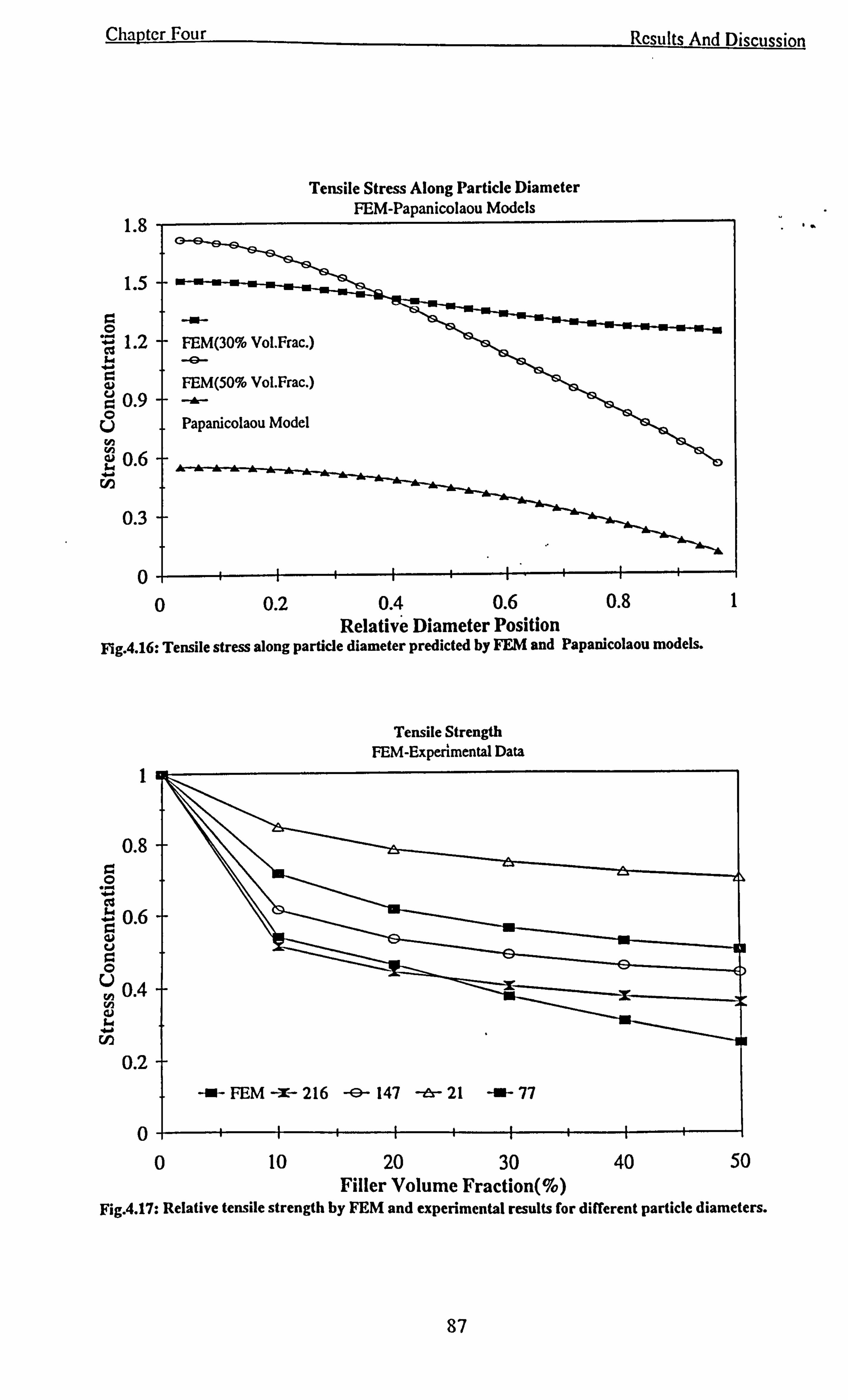
Chapter Four
1.8
I °ýýý-ý 1.5
Tensile Stress Along Particle Diameter FEM-Papanicolaou Models
-a- 0 1.2 FEM(30% Vo1. Frac. )
C43 -ý- FEM(50% Vo1. Frac. )
0.9 -ý- u Papanicolaou Model
0.6 . -ý-ý-. -ý Cl) 1 0.3
Results And Discussion
0 0 0.2 0.4 0.6 0.8 1
Relative Diameter Position Fig. 4.16: Tensile stress along particle diameter predicted by FEM and Papanicolaou models.
Tensile Strength FEM-Experimental Data
1
0.8 0 .., cl ý 0.6
u 0 u ,, 0.4 W c, c,
Cl)
0.2
0 0 10 20 30
Filler Volume Fraction(%) 40 50
Fig. 4.17: Relative tensile strength by FEM and experimental results for different particle diameters.
87
Chapter Four Results And Discussion
4. Schrager (Schrager, 1978):
Qý = Qm exp(-2.66 Vb) (4.9) , I.
The results obtained using the above equations are given in figure 4.15 and are
compared with the results of our model. All of these models except the Neilsen's
model show a decrease in the strength of the composite with increasing volume
fraction of the filler. The Neilsen's predictions depend strongly on the model which is
used to obtain the modulus of the composite at different filler volume fractions.
The finite element model gives rather low tensile strengths for cases corresponding to
the described models. In the finite element analysis, it is assumed that composite failure
occurs when the first element fails. A more realistic. assumption would be that
composite failure does not occur until several of the highly stressed elements fail. This
allows for `crack arrest' by neighbouring inclusions and also takes into account the
statistical increase in the strength for the small volume of material which is subjected
to the stress concentration. The use of this averaging technique will results in an
increase in the theoretical strength of the composite.
Papanicolaou et al (Papanicolaou and Bakos, 1992) have proposed a model for the
prediction of the tensile strength of the particulate filled polymers. They have used a
modified Cox model to find the stress distribution along a particle diameter. The load
which is carried by the inclusions is calculated and used to estimate the tensile strength
of the composite. The variations of the tensile stress concentration along the particle
diameter of the inclusion are presented in figure 4.16. The trend of model predicted
variations is similar to that obtained by Papaicolaou. Although the curve predicted by
the finite element model shows a shift to higher values compared to the curve found
using modified Cox model (Cox, 1952).
The experimental results show that the strength of the composite depends on the size
of the filler particles (London et al, 1977). In figure 4.17 the experimental results for
four different particle diameters, 216 µm, 147 µm, 77 µm and 21 µm are compared
88
Chapter Four Results And Discussion
with our model. It can be seen that for the range of particle diameters studied the
composite strength diminishes at higher volume fractions. The results also indicate
that smaller particles show higher strength. The reason for this phenomenon is not
entirely clear, but the increase in interfacial area per unit volume of filler for smaller
particles must be an important factor. A second factor which may also be important, is
that the stress fields near a particle are independent of the size of the particle,
nevertheless the volume of polymer that experiences a given stress concentration
increases with particle size. Therefore the probability of finding a large flaw within this
volume increases. If a large flaw exists within an area of stress concentration, the
tensile strength will be reduced according to Griffith's theory. In most of the
aforementioned theoretical models, the effect of particle size cannot be investigated. In
our finite element model we also assume that the composite is flawless and hence it
predicts the strength of the composite through the stress fields which are independent
of the particle size. Figure 4.17 confirms once again that our finite element model
provides a somewhat conservative prediction of the strength for the composite.
89
Chapter Four Results And Discussion
4.3 COMPOSITES FILLED WITH DEBONDED RIGID
PARTICLES
Rigid spherical inclusions in glassy polymers induce inhomogeneous stress fields and
thus act as stress concentrators. Consequently, plastic deformation processes such as
craze and shear band are formed at these inclusions. The mechanisms of craze
formation and shear band formation are investigated for small glass spheres
embedded in matrices subjected to uniaxial tension. These microscopic studies have
revealed the profound effect of the degree of interfacial adhesion on the mechanism of
craze (Wellinghoff and Baer, 1978; Donald and Kramer, 1982) and shear band
formation (Kinloch and Young, 1983). In the cases where the adhesion of glass sphere
and polystyrene matrix is perfect, the crazes are found near the poles of the sphere.
From stress analysis around a completely bonded sphere it appears that these are
regions of maximum dilatation and of maximum principal stress. For perfectly adhering
glass spheres in a polycarbonate matrix the shear bands are found to form around the
surface of the sphere at an angle of 45° from the poles defined by the axis of symmetry
of the stressed sphere. These are regions of maximum distortional strain energy density
and maximum principal shear stress. In the case of poor interfacial adhesion between
the glass sphere and the polymer matrix, both craze and shear band formation are
found to be preceded by dewetting along the interface between sphere and matrix.
During dewetting a curvilinear interfacial crack is formed, starting at the pole and
propagating along the interface in the direction of the equator until, at an angle of
about 60° from the pole, a craze or shear band originates at the tip of this crack. The
results of these studies prompted us to analyse the stress conditions near the tip of a
curvilinear interfacial crack between a glass sphere and a polymer matrix.
4.3.1 Boundary conditions at the interface
Figure 4.8a indicates that for all volume fractions of the filler the normal stress has
negative value and is compressive in the part of the interface which starts from the
equator and ends at about 0 =22°. At this point the normal stress is about zero and
from this point towards the pole of the particle it continues to rise to its maximum
90
Chapter Four
I E-03
C7 6E-04
ev
... A P8
cl 2E-04
94
0 Matrix n
Filler
41. 0 or 410
. Ppý,
0 0
0 0
0 0
0 Illb
Results And Discussion
0 40 0 0 I 4p 0
,,;;, dwtýý6568& 6&A& -- -- -- - A, "A---
-2E-04 ý--{
0 20
I
40 60 80 Angle(Degree)
jg. 4.18: Radial displacement of the matrix and filler at the interface of the partly debonded particle
Interfacial Radial Stress Filler Volume fraction(10%)
0.5
0.3
0 .., cl 10.1
0
0
op w
0
ýoa1
aý c, 1 +ý ý Ln
-0.3t m
a
0000
0 Matrix
Filler
-0.5 0 20 40 60 80
Angle(Degree)
Fig. 4.19: Radial stress concentration of matrix and filler at the interface of a partly debonded particle
Interfacial radial displacement Filler Volume fraction (10%)
91
Chapter Four Results And Discussion
value at the pole. From this analysis it can be concluded that in the case of debonded
filler or when dewetting occurs in a bonded filler, from the pole up to a length of the
unbonded region represented by 0 =22°, the entire unbonded region may be regarded
as an interfacial crack.
Here we consider two cases. In the first case the remainder of the interface is bonded
and there is no relative displacement of the matrix. In the second case we investigate
the situation in which all the interface is debonded and from 0 =22° to the equator of
the particle there can be a relative tangential displacement of the matrix depending on
the frictional force at the interface. If the frictional force acting on the interface is high
enough it can prevent the particle and matrix to have relative tangential movement.
Therefore under this condition the model will be similar to the first case. If the
frictional force is weak the tangential displacement occurs and hence slip boundary
condition is imposed for this case. The slip coefficient controls the extent of relative
movement of the matrix and the filler particle.
4.3.2 Displacement
Figure 4.18 shows the normal displacement of the filler and the matrix at the interface.
The radial displacement of the matrix and the filler from the equator to 0 =22° is
negative and much smaller than the displacement of the other segment of the
interface(nearly zero). This negative value confirms that even in the case of debonding
of the filler at this part, the two phases remain in contact and the stress can be
transferred from the matrix to the filler. From the point of 8=22° to the pole the radial
displacement of the matrix is positive and increases to its maximum at the pole. The
filler displacement in this part is nearly zero.
4.3.3 Interfacial stresses
The interfacial radial stress concentration in matrix and filler is shown in figure 4.19
for volume fraction of 10%. The results indicate that the normal stress is negative and
compressive at the interface from the equator (i. e. 0=0) to 0=22°. In higher volume
fractions this stress become closer to zero. The normal stress concentration has its
92
Chapter Four
Interfacial radial displacement Filler Volume fraction (10%)
I E-03 0
Matrix
Filler 6E-04
co -
a rA ... Pý ý ýö 2E-04 cl ts:
-2E-04 4 0
1--{
20
'0 19
.. r . -10
410 0
0 lb
0 0
. 0
Results And Discussion
0 .
410 0 0 4D
0
40 60 Angle(Degree)
ý-ý
80
Fig. 4.18: Radial displacement of the matrix and filler at the interface of the partly debonded particle
Interfacial Radial Stress Filler Volume fraction(10%)
o. s 0
Matrix 0.3
Filler 0 .r ý ý wv ýý
W 0.1 + r. v
u CýO00000000
ýo0
ýW .. cn -0.3 1
-0.5
m
0 20 40 60 80 Angle(Degree)
Fig. 4.19: Radial stress concentration of matrix and filler at the interface of a partly debonded
particle
a
93 (: ý
Chapter Four
5
4.5+
4.
p 3.5 -I- 0
0
0
cl 3
u 2.5 uýo u2 0 J 1.5 CROI C3 W ý1
_ý o .r+ Q2 --
'°` " 0.5 t
ol -0.5 ý
v
-1 0 20 40 60 80
Angle(Degree)
Fig. 4.20: Tangential stress concentration of matrix and filler at the interface of the partly denonded Particle
VonMises Stress at the interface Filler Volume fraction(10%)
7-- 6.5
6-- 5.5
5 .., 4.5 4. A 4
3.5 Ü3
2.5 2
Ln 1.5
1
0.5
0 0
0
0 x CRI
0 x
Tangential stress concentration Filler Volume fraction(10%)
Results And Discussion
0 Matrix X
Filler
Qýýgxxxx 0000
X
0 0X
c9l X O
20
0
Matrix x
Filler
0 0
° 00 xxxQ25xxg25S2Pxxxx . ýo.. .ý
40 60 Angle(Degree)
80 100
Fig. 4.21: Von Mises stress concentration of matrix and filler at the interface of the partly debonded
particle
93
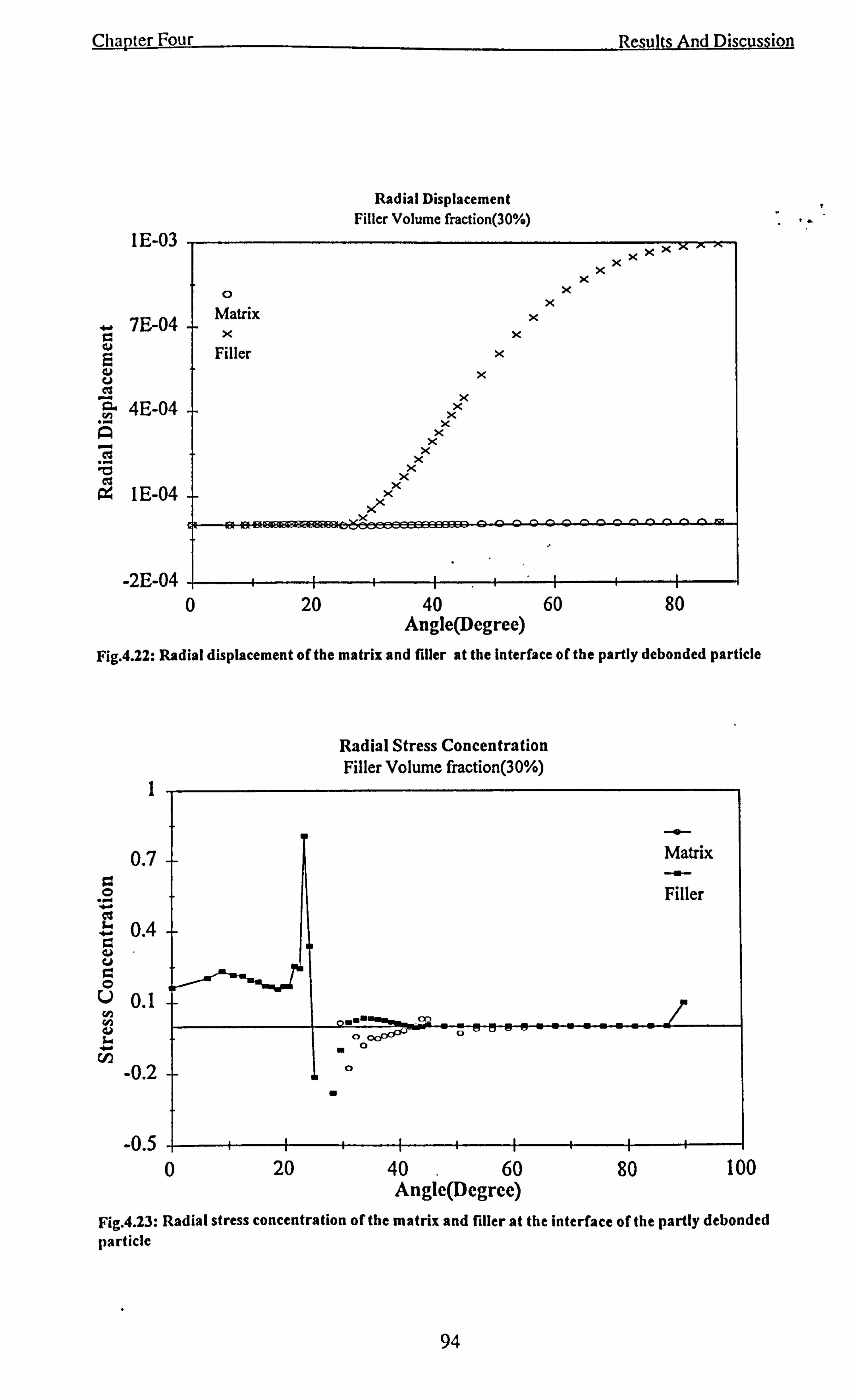
Chapter Four
Radial Displacement Filler Volume fraction(30%)
I E-03
ý 7E-04 I aý E u cts a ý ... A
-
4E-04 -4-
cý ýä 0 a1 E-04
0 Matrix
X Filler
Results And Discussion
XX X
X
x x
X X
X X
X X
X X
X X
X X
ý
X X
X
X
xx R ý
a0----00^00----------
-2E-04 1Fi&i. 21 ---4
0 20 40 60 Angle(Degree)
-{- 80
Fig. 4.22: Radial displacement of the matrix and filler at the Interface of the partly debonded particle
Radial Stress Concentration Filler Volume fraction(30%)
0.7 -I-
-0-
Matrix -+. - Filler
0.44-
0.1
-0.2 4-
own"'-ow`
a 0
0
a
0 z
0 20 40 60 80 100 Angle(Degree)
Fig. 4.23: Radial stress concentration of the matrix and filler at the interface of the partly debonded
particle
94
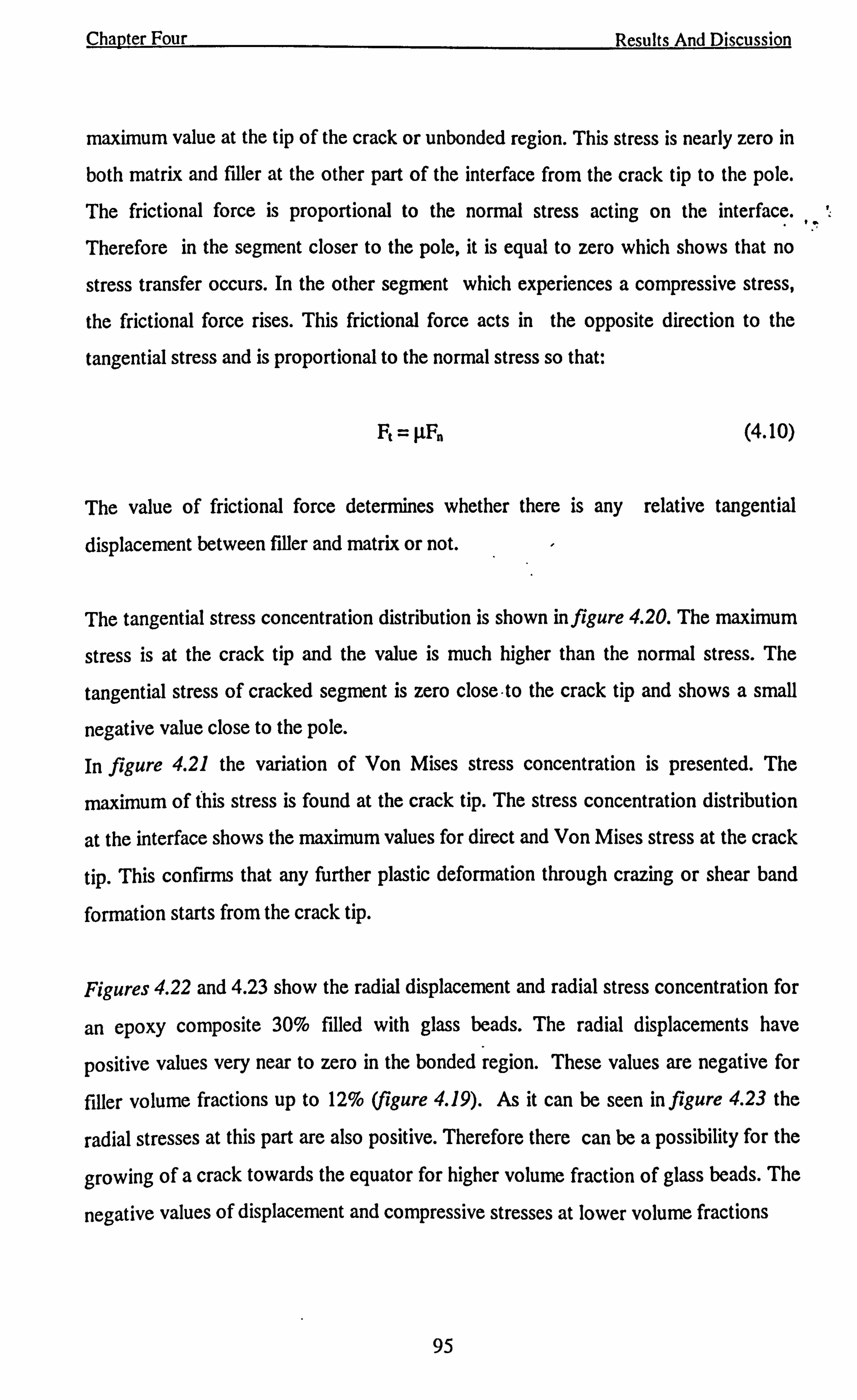
Chapter Four Results And Discussion
maximum value at the tip of the crack or unbonded region. This stress is nearly zero in
both matrix and filler at the other part of the interface from the crack tip to the pole.
The frictional force is proportional to the normal stress acting on the interface.
Therefore in the segment closer to the pole, it is equal to zero which shows that no
stress transfer occurs. In the other segment which experiences a compressive stress,
the frictional force rises. This frictional force acts in the opposite direction to the
tangential stress and is proportional to the normal stress so that:
Ft = J. LF. (4.10)
The value of frictional force determines whether there is any relative tangential
displacement between filler and matrix or not.
The tangential stress concentration distribution is shown in figure 4.20. The maximum
stress is at the crack tip and the value is much higher than the normal stress. The
tangential stress of cracked segment is zero close. to the crack tip and shows a small
negative value close to the pole.
In figure 4.21 the variation of Von Mises stress concentration is presented. The
maximum of this stress is found at the crack tip. The stress concentration distribution
at the interface shows the maximum values for direct and Von Mises stress at the crack
tip. This confirms that any further plastic deformation through crazing or shear band
formation starts from the crack tip.
Figures 4.22 and 4.23 show the radial displacement and radial stress concentration for
an epoxy composite 30% filled with glass beads. The radial displacements have
positive values very near to zero in the bonded region. These values are negative for
filler volume fractions up to 12% (figure 4.19). As it can be seen in figure 4.23 the
radial stresses at this part are also positive. Therefore there can be a possibility for the
growing of a crack towards the equator for higher volume fraction of glass beads. The
negative values of displacement and compressive stresses at lower volume fractions
95
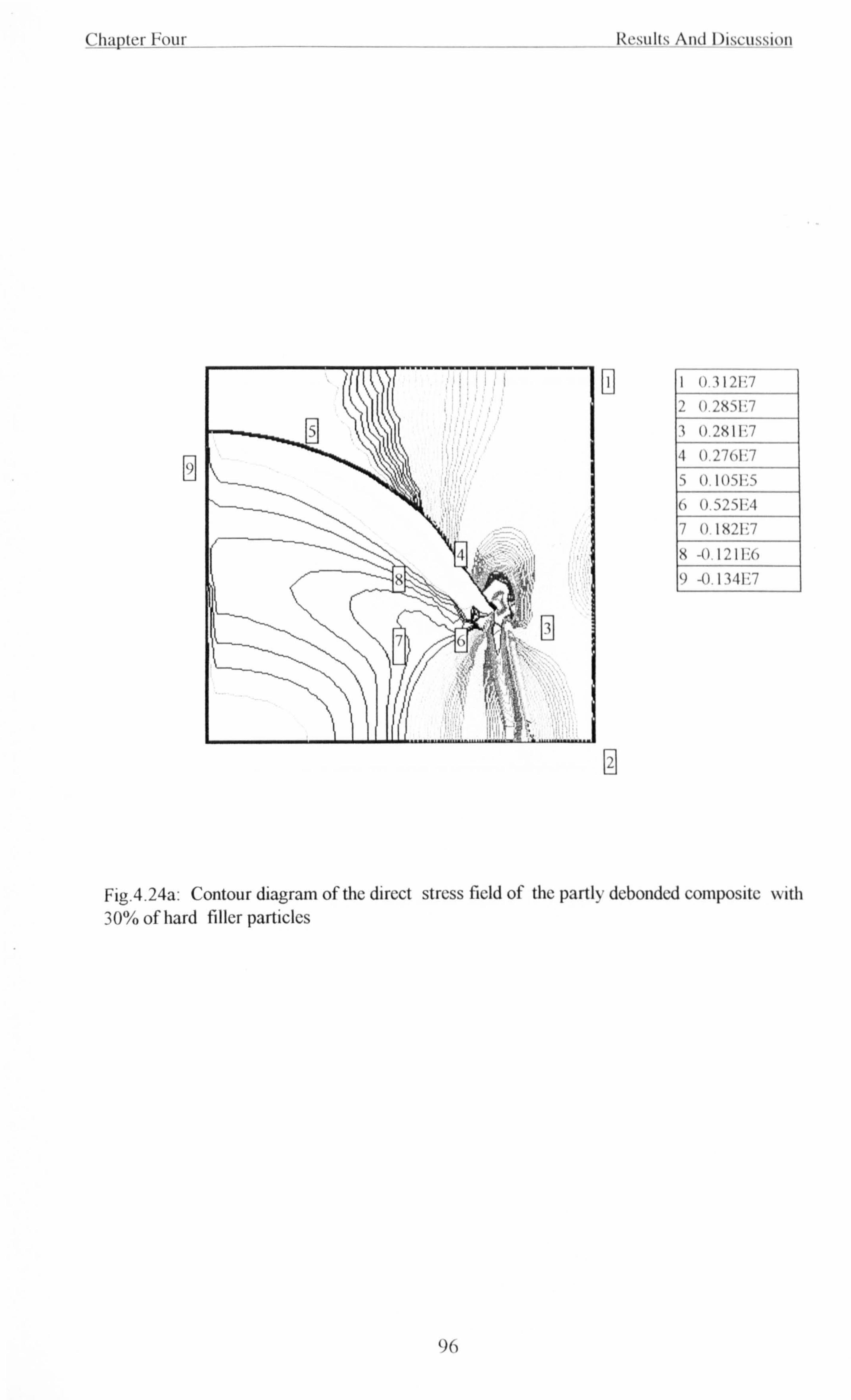
Chapter 1=our Itrsulls And I )iscUSsilln
I 0.3121? 7
2 0.2x51i7 3 0.2KI1? 7
4 0.27GV17
5 0.1051? 5
(, O. 5251; 4
7 O. 1H2i? 7
K -0.121F. 6 l)
-0.1341`7
L
Fig. 4.24a: Contour diagram of the direct stress field of the partly debonded composite with 30% of hard filler particles
96
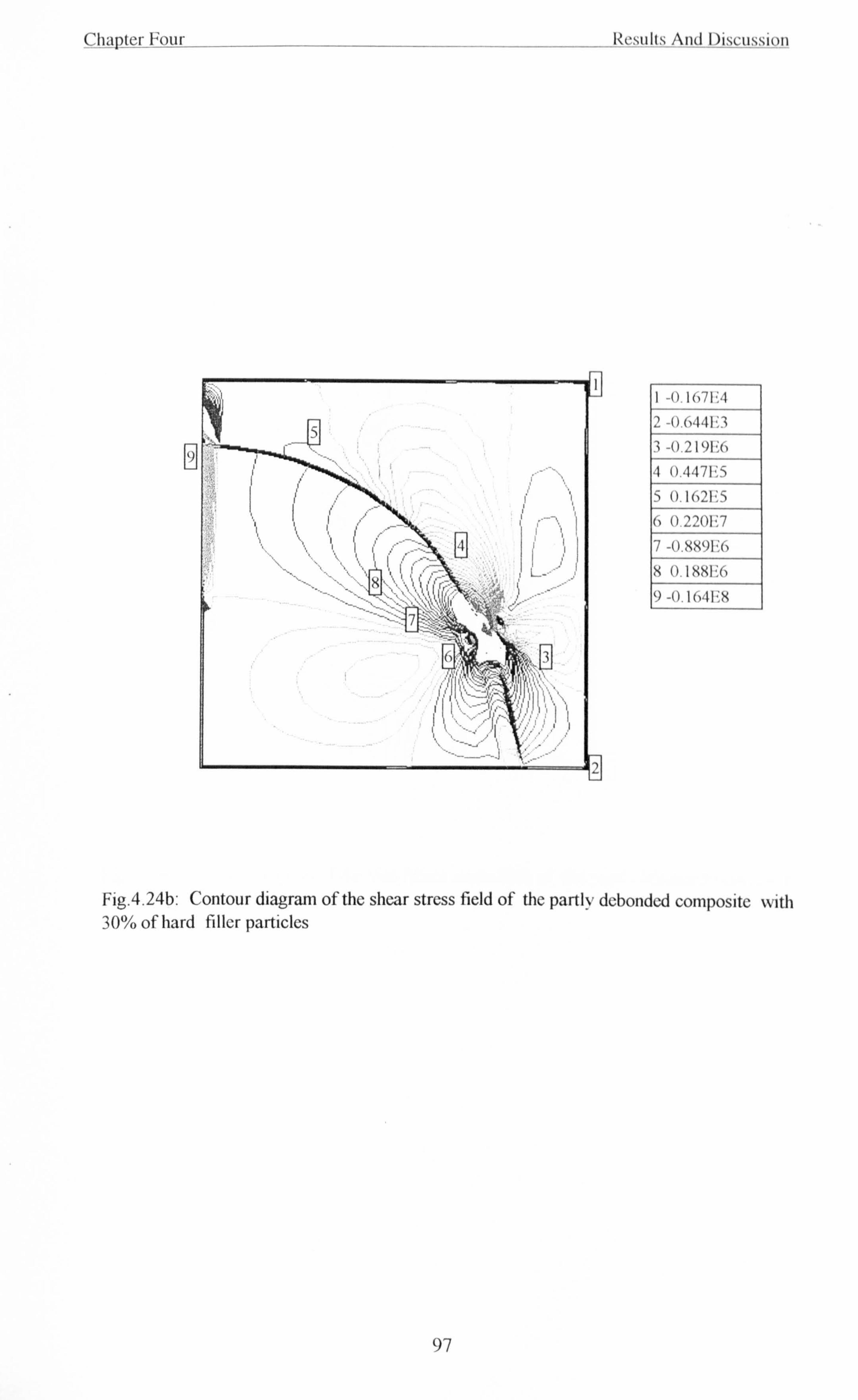
Chapter-Four Results And Discussion
9
1 -0.1(171{4 2 -U. G441; 3
3 -U. 2191; C,
4 t1.4471? 5
5 0.102F5 6 0.2201; 7
7 -0. KK9F6 8 0.1 Rfi1? C, 1%
-(). 1o"11: K
Fig. 4.24b: Contour diagram of the shear stress field of the partly debonded composite with 30% of hard filler particles
97
Chapter Foul.
H
Kxsulis And 1 )isCussi0n
I 3.121 '06
2 2. x51'+06
3 2. x5I'+05
4 2.851 '106
5 5.251'+05 6 6.771'+06
7 2,241,1+06
x 4. x11'+05
3.2nI". M7
Fig. 4.24c: Contour diagram of the Von Mises stress field of the partly debonded composite with 30% of hard filler particles
98
Chapter Four
Radial Stress Concentration Slip At The Interface(V-10%)
0.5
0.34-
0.1 -ý
a
m
0
Results And Discussion
0 Matrix 0
Filler
.
ýý 'ý -apr. v C] v lJ vv... --- -i ýo
oýdýr -ý. 1 ý
ab
-0.3 -ý
-0.5 0
0 000000
0 20 40 60 80 Angle(Degree)
Fig. 4.25: Radial displacement of the matrix and filler at the interface of the partly debonded particle with slip condition at the closed segment of the interface
Tangential stress concentration Slip At The Interface(Vf=10%)
5
4.5-
4-
3.5 0 w3 ý 2.5
u2
1.5
1 C;
r 0.5 -4
0 Matrix x
Filler
fo C) n
-0.5 t _°OOo
ii iý 0 20 40 60 80 100
Angle(Degree)
Fig. 4.26: Tangential stress concentration at the interface of partly debonded particle with slip condition at the closed segment of the interface
CRI
0
0
o ý0
0
99
Chapter Four Results And Discussion
VonMises Stress Concentration Slip At The Interface(Vf=10ßö)
5--
4.5--
4--
3.5--
3--
2.5--
2--
1
0.5
0
-0ý5 }
1
0
0
0
0
0 ca 0
0 0
ý ý ý
x
O
O 0
0 Matrix x
Filler
-0000 ýo 00
0 20 40 60 80 100 Angle(Degree)
Fig. 4.27: VonMises stress concentration at the interface of partly debonded partilce with slip condition at the closed segment of the interface.
1E-03
ý 6E-04
d»
Matrix A
5 u cl a ý .., A 2E-04 +
Filler
Interfacial Radial Displacement Slip At Interface(Vf=10%)
0
e 10 0
. 40
0
40 0
0 0
4D 0
a a 0
0 0 00
49 Ift Ift IN N
-2E-04 0 20 40 60
Angle(Degree) 80
Fig. 4.28: Radial displacement of the matrix and filler at the interface of the partly debonded particle with slip condition at the closed segment of the interface
100
Chapter Four
0.5
0 0
0.3
.., .r
m
ý 0.1 ý --' . Fi - ---
Results And Discussion
0 Matrix
Filler
,o --- ---m m u 19 o
N -0.1 ý
to) a) &. En
-0.3-F 0
Radial Stress Concentration Slip at the interface(Vf=30%)
0
-0.5 -ý ---I IIIII
0 20 40 60 80 Angle(Degree)
Fig. 4.29: Radial displacement of the matrix and filler at the interface of the partly debonded particle with slip condition at the closed segment of the interface
Modulus of Composite with Debonded Filler Particle or Void
3.5E+09 -i
3.0E+09
ä, 2.5E+09 v h
0 b 2.0E+09 0
1.5E+09 0
E ul 1.0E+09 -a-
} Debonded particle filled composite
5.0E+08 -0-
Porous Composite
O. 0E+00 I --ý--+ 0 10
ý -}- 20 30
f
Volume Fraction(%)
Fig. 4.30: Modulus of composite filled with debonded filler particle or void
H- 40
4
50
Iw
101
Chapter Four Results And Discussion
exclude the possibility of growing or opening of the crack further than 0 =22° towards
the equator.
The contour diagrams of the direct stress, shear stress and Von Mises stress
concentrations are shown in figure 4.24a-c. Maximum stress concentration in all of
the above cases can be found at the crack tip.
4.3.3 Slipping of the particle at part of the interface
Figures 4.25-28 show the stress and displacement variations at the interface for epoxy
composite filled with 10% of glass beads while slip condition is imposed on the
segment of the particle from 0 =22° to the equator. Since a low slip coefficient is
used, the stress and displacement fields follow more or less the same trend as the no
slip case. However, the maximum radial, tangential and Von Mises stresses decrease
compared to the non slip case. Using the same slip coefficient in a composite with 30%
volume fraction of filler the results are shown in figure 4.29. The stress concentrations
shows noticeable decrease at this volume fraction.
In figure 4.30 the modulus of the composite filled with the unbonded particles and the
composite containing voids are compared for the range of volume fractions.
4.3.4 Strength
The tensile strength of the composites with perfectly bonded and unbonded interfaces
and composites with voids are calculated using finite element model. The results are
compared in figure 4.31. The decrease of the tensile strength with increasing volume
fraction can be observed in all cases. The graph shows the strength of composite with
unbonded interface is between the upper bound curve which is for the bonded
interface and the lower bound curve which represents the composites with voids.
In figure 4.32 the strength predicted by the finite element analysis is compared with the
following models proposed by Neilsen and Nicloais&Narkis.
Different theoretical models are suggested for the unbonded or no adhesion case. A
commonly reported model is due to Nicolais and Narkis (Nicolais and Narkis, 1971)
which is based on the assumption that the unbonded particle cannot carry any of the
102
Chapter Four Results And Discussion
load and the yielding occurs in the minimum cross section of the continuous phase.
They presented the following equation for the yield stress of the composite.
6c =am(1-1.21Vf) (4.11)
Another model suggested by Neilsen ( Neilsen, 1966) gives the yield stress in a
composite assuming no adhesion between polymer and filler, expressed as :
6c = Q. (1- V f')S (4.12)
where S is the stress concentration function which can be determined by the finite
element analysis. The Neilsen's prediction is very close to the finite element prediction
for voided composites and it is also closer to the unbonded composite. But the
Nicolasis and Narkis's model gives a much higher values for the strength.
103
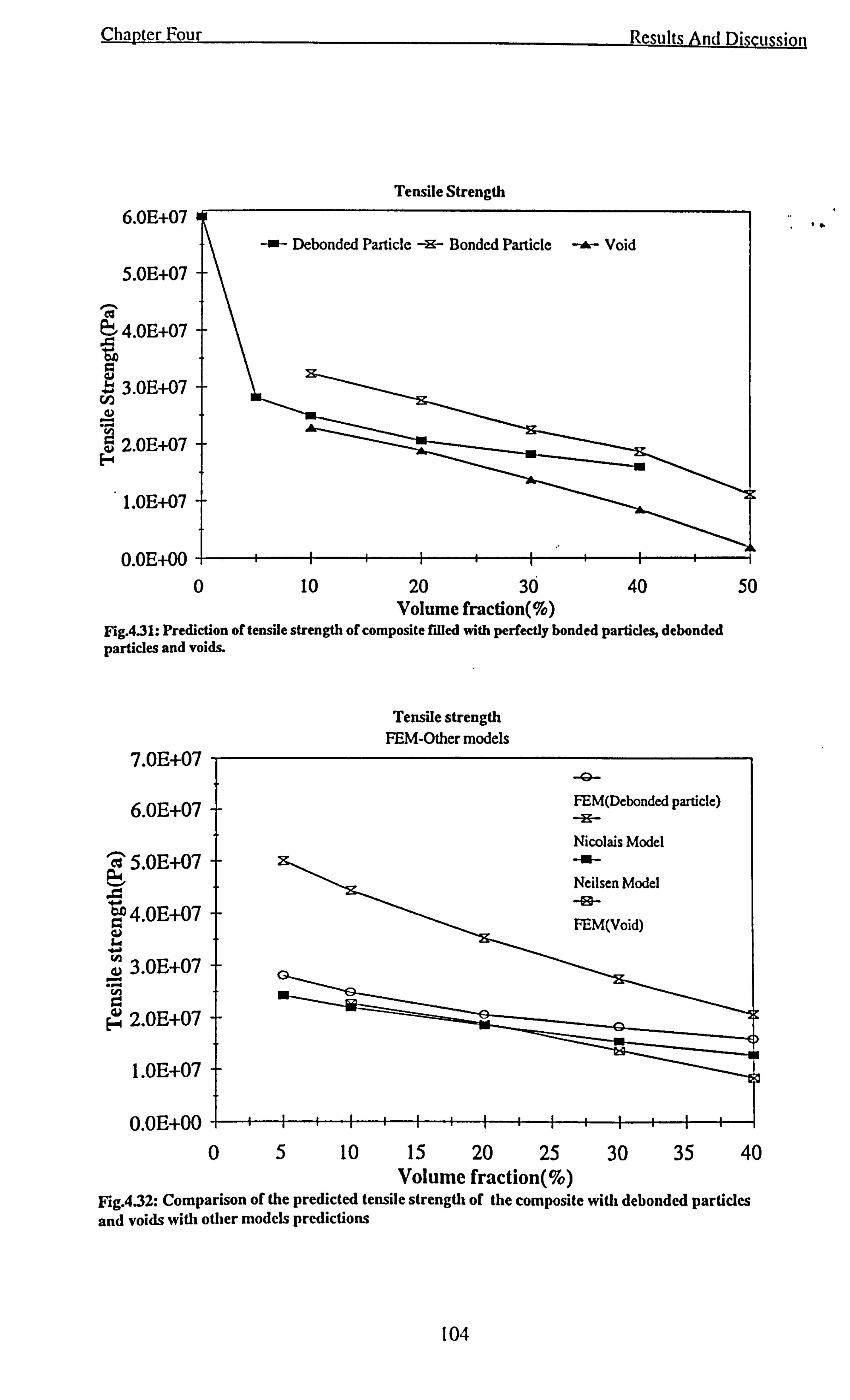
Chapter Four
5.0E+07
, -. '- 4.0E+07
P= a a, w 3.0E+07
cn d r.. ..,
0 10
Tensile Strength
20 30 Volume fraction(%)
Results And Discussion
40
Fig. 4.31: Prediction of tensile strength of composite filled with perfectly bonded particles, debonded particles and voids.
Tensile strength FEM-Other models
7.0E+07 i
6.0E+07
5.0E+07
ý 4.0E+07 (V kg
3.0E+07 ý ... ý ý F, 2.0E+07
1.0E+07
-a- FEM(Dcbonded particle)
50
0.0E+00 E++i-+-i II1 11 i1 --ý 1 05 10 15 20 25 30 35 40
Volume fraction(%) Fig. 4.32: Comparison of the predicted tensile strength of the composite with debonded particles and voids with other models predictions
104
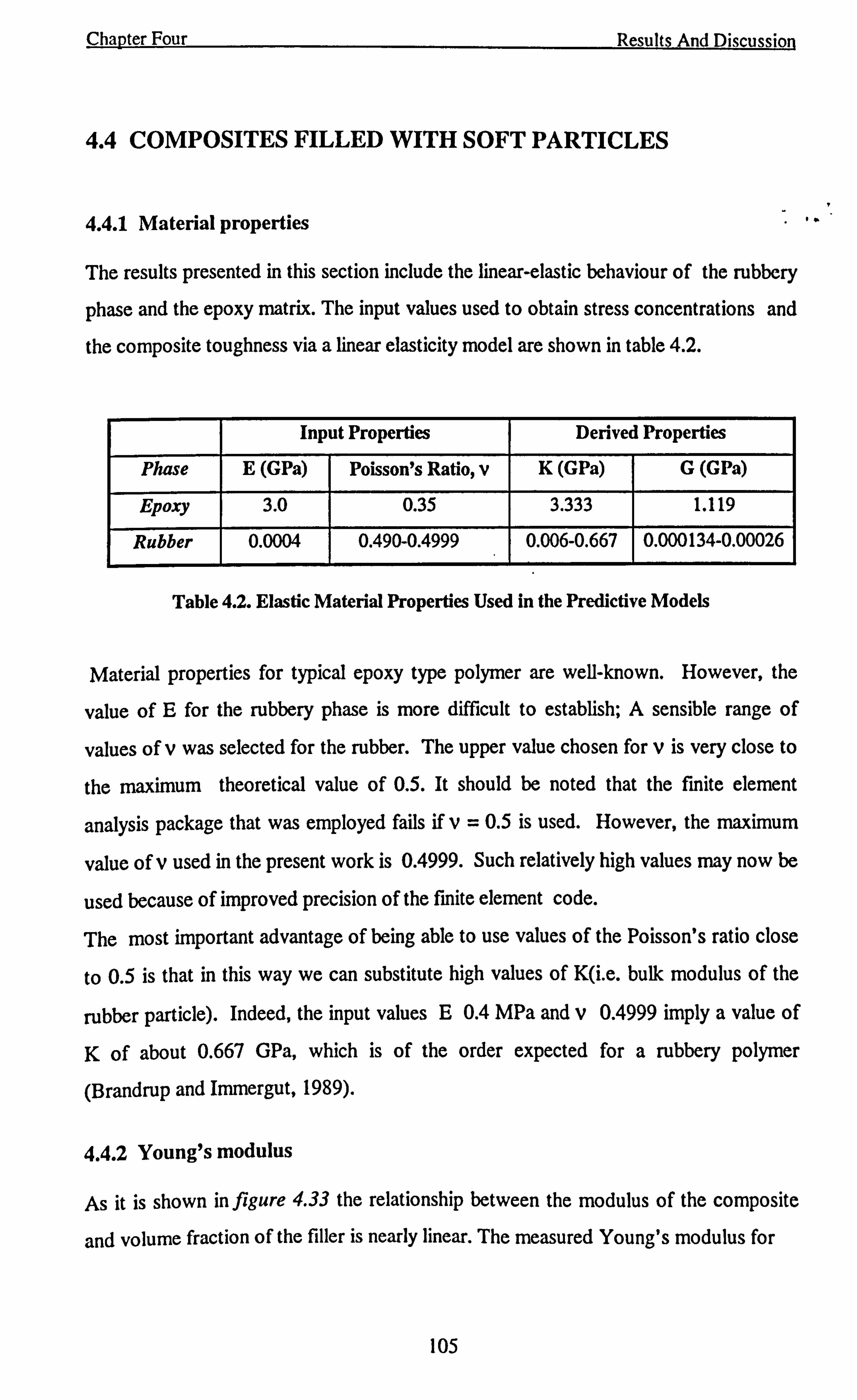
Chapter Four Results And Discussion
4.4 COMPOSITES FILLED WITH SOFT PARTICLES
4.4.1 Material properties
The results presented in this section include the linear-elastic behaviour of the rubbery
phase and the epoxy matrix. The input values used to obtain stress concentrations and
the composite toughness via a linear elasticity model are shown in table 4.2.
Input Properties Derived Properties
Phase E (GPa) Poisson's Ratio, v K (GPa) G (GPa)
Epoxy 3.0 0.35 3.333 1.119
Rubber 0.0004 0.490-0.4999 0.006-0.667 0.000134-0.00026
Table 4.2. Elastic Material Properties Used in the Predictive Models
Material properties for typical epoxy type polymer are well-known. However, the
value of E for the rubbery phase is more difficult to establish; A sensible range of
values of v was selected for the rubber. The upper value chosen for v is very close to
the maximum theoretical value of 0.5. It should be noted that the finite element
analysis package that was employed fails if v=0.5 is used. However, the maximum
value of v used in the present work is 0.4999. Such relatively high values may now be
used because of improved precision of the finite element code.
The most important advantage of being able to use values of the Poisson's ratio close
to 0.5 is that in this way we can substitute high values of K(i. e. bulk modulus of the
rubber particle). Indeed, the input values E 0.4 MPa and v 0.4999 imply a value of
K of about 0.667 GPa, which is of the order expected for a rubbery polymer
(Brandrup and Immergut, 1989).
4.4.2 Young's modulus
As it is shown in figure 4.33 the relationship between the modulus of the composite
and volume fraction of the filler is nearly linear. The measured Young's modulus for
105
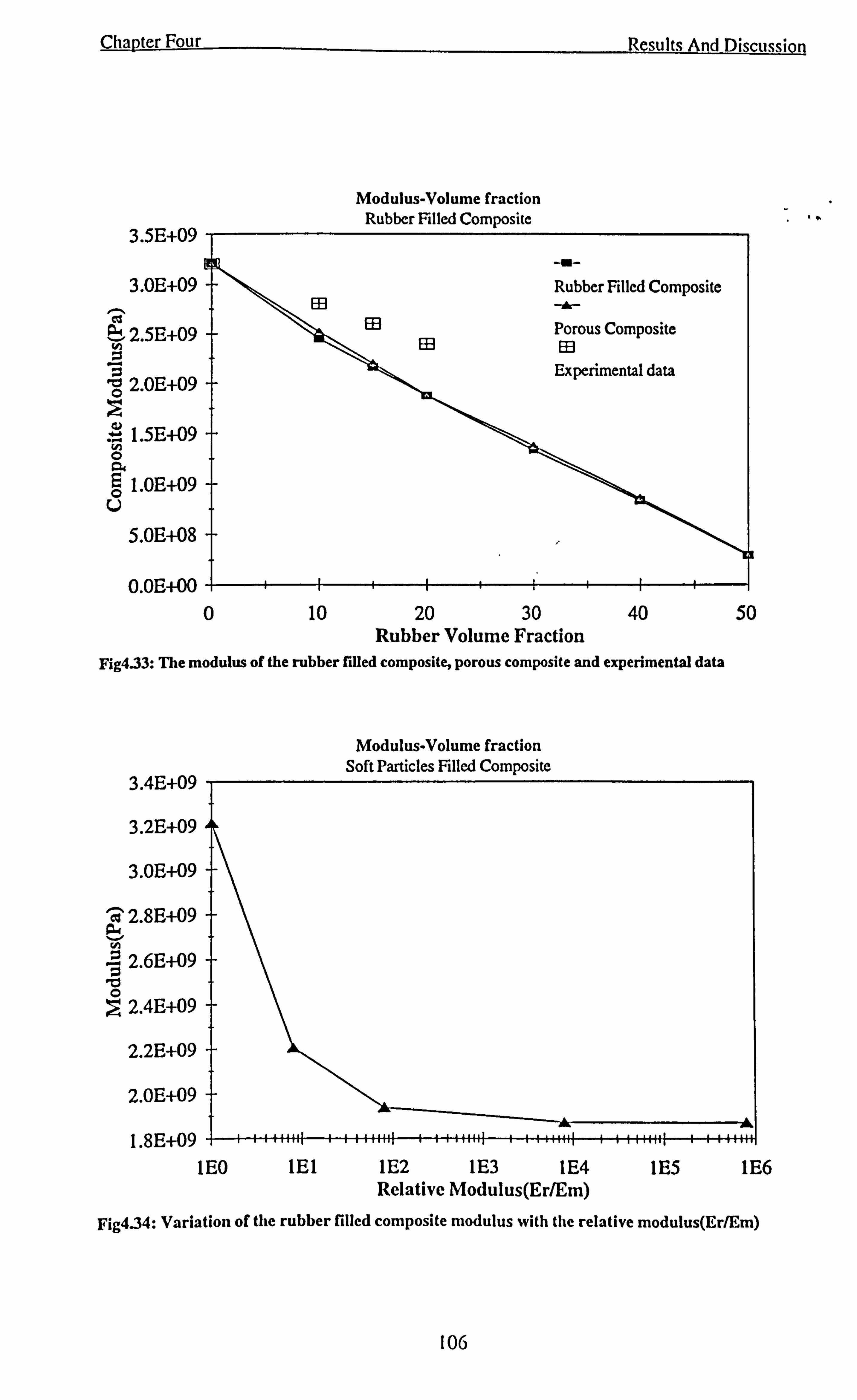
Chapter Four
3.5E+09
ý a' 2.5E+09 (I, ý
ý. c 2.0E+09
1.5E+09
1.0E+09 U
5.0E+08
0.0E+00 -+ 0
} -{- 10
Results And Discussion
Modulus-Volume fraction Rubber Filled Composite
-As-
ED
f
03
t {
Rubber Filled Composite -A- Porous Composite 133 Experimental data
50 20 30 Rubber Volume Fraction
ý H- 40
1
Fig4.33: The modulus of the rubber filled composite, porous composite and experimental data
Modulus-Volume fraction Soft Particles Filled Composite
'2 2.8E+09
2.6E+09
ý 2.4E+09
2.2E+09
2.0E+09
Al 1.8E+09 TIII111111III1 III HII111111III111111III111111 iI I 12 1 11E0
1E1 1E2 1E3 1E4 1E5 1E6 Relative Modulus(Er/Em)
Fig4.34: Variation of the rubber filled composite modulus with the relative modulus(Er/Em)
Iw
106
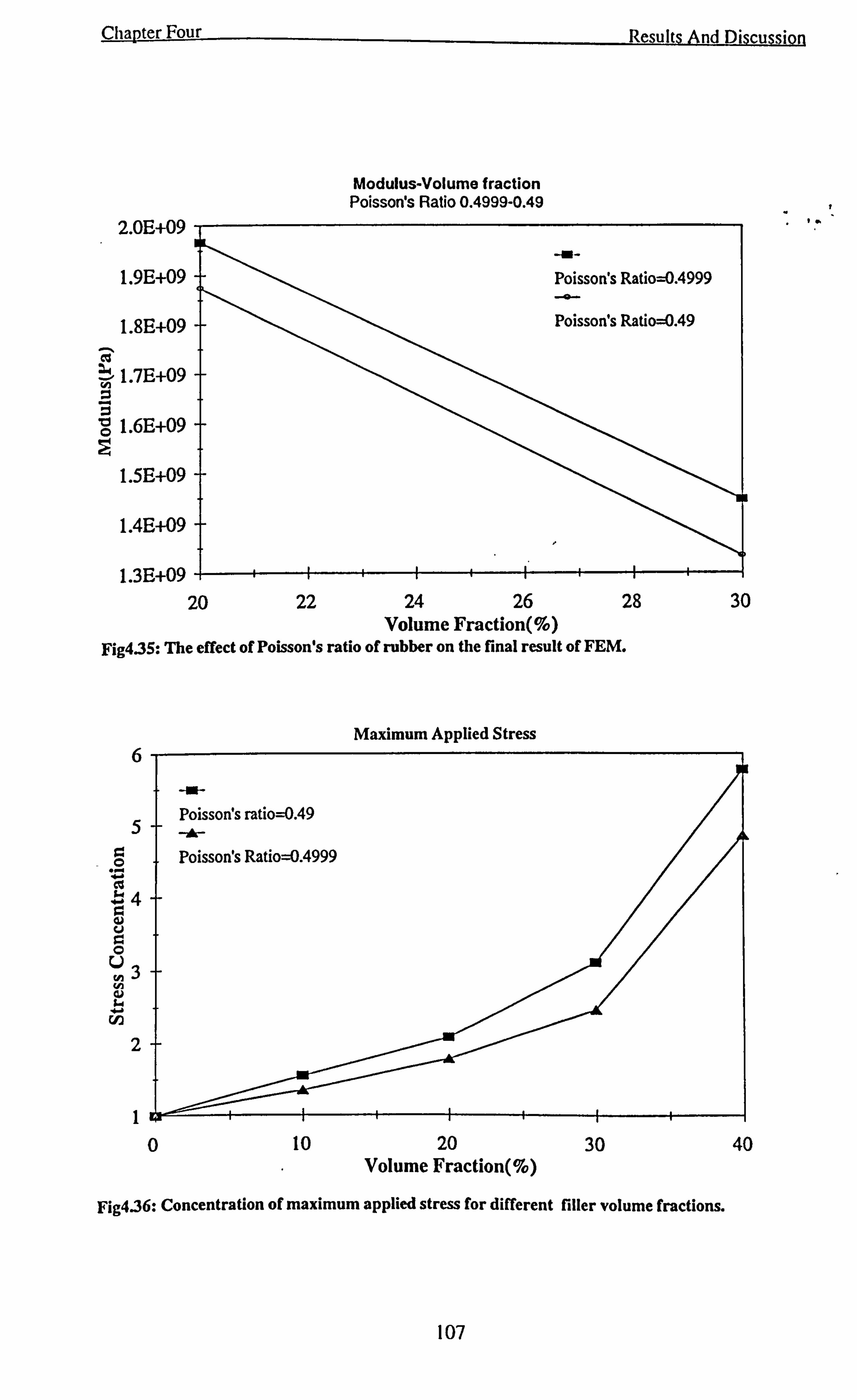
Chapter Four
Modulus-Volume fraction Poisson's Ratio 0.4999-0.49
2.0E+09
1.9E+09
1.8E+09 . -I cl ý 1.7E+09 0 ý c
1.6E+09 t ý
1.5E+09
1.4E+09
1.3E+09 20
i H- 22
f I i
-m-
Results And Discussion
Poisson's Ratio=0.4999 _a- Poisson's Ratio=0.49
24 26 Volume Fraction(%)
f
28
Fig4.35: The effect of Poisson's ratio of rubber on the final result of FEM.
6
0 ... cl
5+
ý4+ m Q u 0 rý r
2+
0 10
Maximum Applied Stress
20 Volume Fraction(%)
30
4
Fig4.36: Concentration of maximum applied stress for different filler volume fractions.
-at- Poisson's ratio=0.49 -, - Poisson's Ratio=0.4999
30
40
107
Chapter Four Results And Discussion
epoxy resin reinforced with 15% volume fraction of rubber spheres is also included.
The measured value is significantly higher than the predicted range by our model. The
lack of precise agreement between experimental and numerical results could arise from the inaccuracy in description of the rubber properties and the assumption that the
phases are perfectly separated. Beyond a volume fraction of about 0.2, there are no
experimental data available for comparison, because when higher concentrations of
rubber are used, phase inversion of the multiphase polymer normally occurs.
Figure 4.34 shows predictions of our model for the Young's modulus of the
multiphase rubber-toughened epoxy as a function of log(Em/Er), where Ep and Em
are the Young's modulus of the rubber and epoxy respectively. A volume fraction of
20% has been assumed for the rubber phase. In the calculations, the Poisson's ratio of
the rubber is considered to be 0.49. Initially the Young's modulus of the two phase
material decreases sharply with an increase in the value of log(Em/Er). When this
value approaches 3.0, the Young's modulus has a constant lower bound of 1.87 GPa.
The predicted values of the overall modulus are relatively insensitive to the changes of
the value of the rubber modulus.
The predicted overall modulus is found to increase by 5% at 20% volume fraction and
7% at 30% of volume fraction if the Poisson's ratio of the rubber is increased from the
value used 0.49 to 0.4999 as is shown in figure 4.35. Therefore the properties of
rubber could probably be best described using a Poisson's ratio of 0.5, but this causes
a problem for the finite element analysis.
The experimental values reported for rubber filled composites are in comparison higher
than our model predictions, this is probably because of some stiffening of the rubber
via the epoxy, the inadequate description of the Poisson's ratio of the rubber in the
model, and incomplete phase separation leading to a lower rubber volume fraction than
the expected theoretical value. The onset of plasticity during the experimental
measurements as well as any experimental errors can also cause some discrepancy
between the measured and the predicted values. In some cases the reason for the
108
Chapter Four Results And Discussion
experimental value to be higher than the predicted results can be the skin effect. The
restrictions imposed by the walls of molds, leads to an excess polymer at the surface of
the test specimens. Thus, in torsion or flexural tests where the maximum stress is at
the surface, the properties of the surface is dominant and determine the behaviour of rw
the whole sample. This error can be corrected by using thicker specimens which can be
extrapolated to infinite thickness, or by using particles of smaller size and extrapolation
to zero particle size. The skin effect can produce errors as large as ten to twenty
percent depending on the thinness of the specimen.
Despite the discrepancy between the experimental and the model results, it should be
noted that almost linear relationship between Young's modulus and volume fraction is
very similar to the relationship measured experimentally by Yee and Pearson.
4.4.3 Stress distribution
4.4.3.1 Concentration of direct stress
The contour diagrams of the direct stress, shear stress and Von Mises stress
concentrations are given infgures 4.37a-c.
The contour diagram for the concentration of the applied stress indicates that the
maximum stress concentration is found at the interface at the equator of the sphere.
The examination of other contour diagrams confirms that this is the maximum principle
stress predicted in the system. The position of maximum stress concentration, at the
equator of the sphere, is in agreement with previous theoretical predictions and
experimental results (Spanoudakis and Young, 1984). As it can be seen in figure 4.36
the values of the maximum stress concentration, varies sharply with the volume
fraction of rubber spheres. The stress concentration decreases with increasing Poisson
ratio of rubber, since the effect of the difference between matrix and physical
properties of the particle is diminished. In figure 4.36 the direct stress concentration
versus volume fraction can be compared for rubber Poisson's ratios, of 0.49 and
0.4999.
109
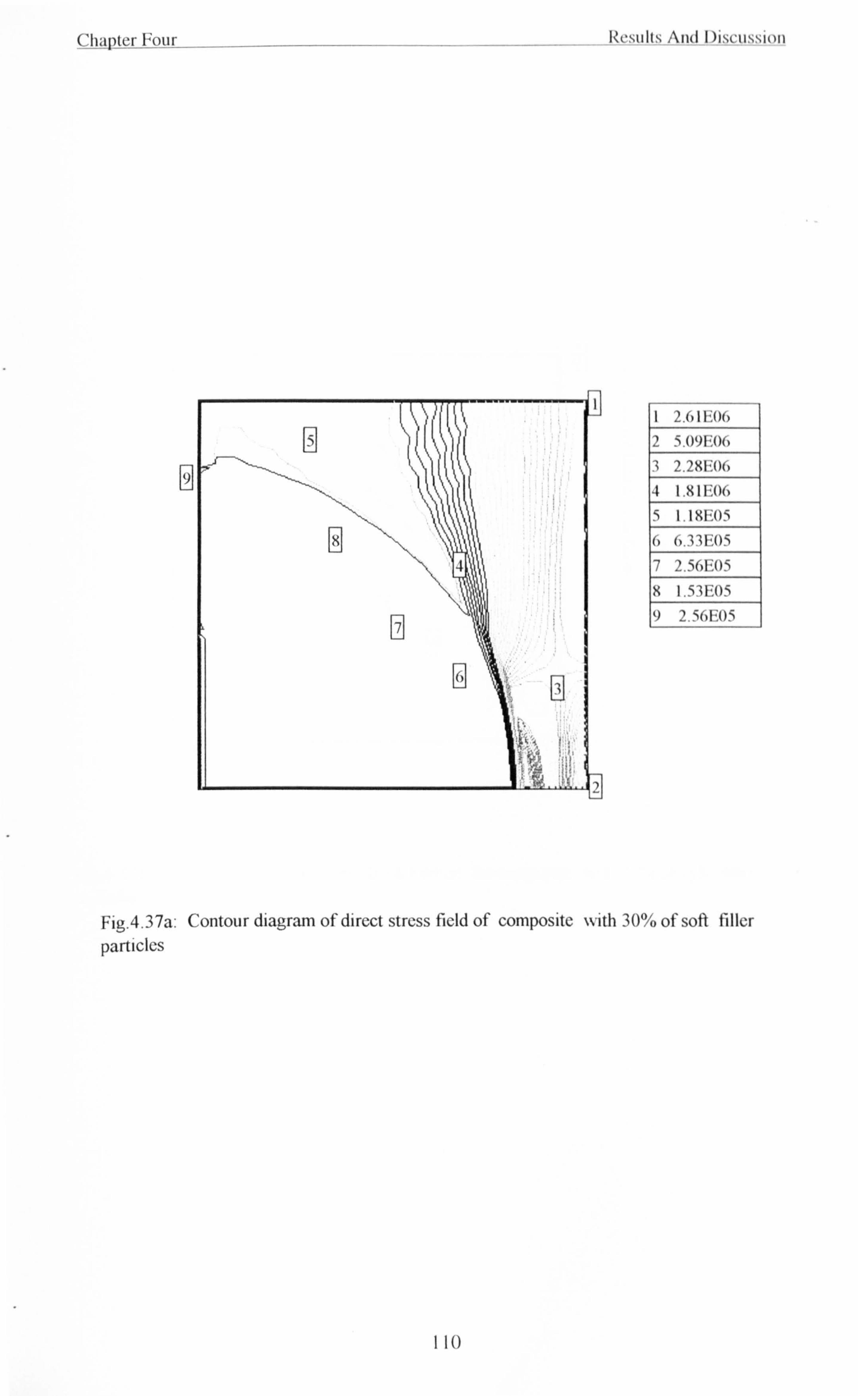
Chapter Four Results And Discussion
H
I 2.61E00
2 5.09F, OG
3 2.2RFO6
4 1. R 1 IA6
1.1 8F. 05
6 (i. 33EO5
7 2.56E05
8 1.53E1)5
9 2.5(, E05
Fig. 4.37a: Contour diagram of direct stress field of composite with 30% of soft filler
particles
110
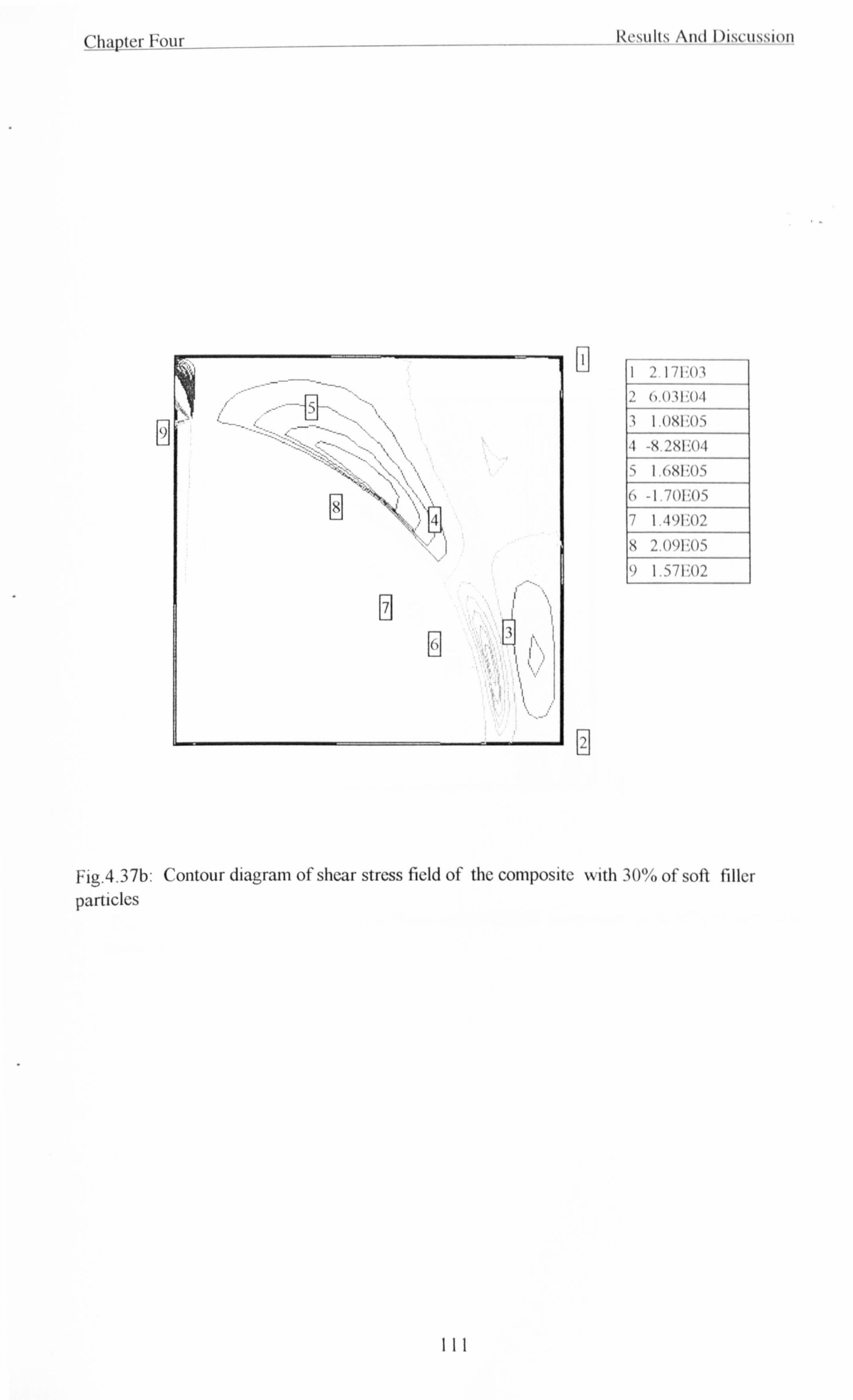
Chapter Four
()
0
6
i
EL i
i ý, ýý.
C1]
I
hrýull` And I )iSruIIsi(, n
2 I7FO3
2 31 -: U4
LOX] ? 05
Ix 2xi; c)a I_6x1-'05
o -1.701? 05
7 1.4')º? 02
x 2.091`. 05
Fig. 4.37b: Contour diagram of shear stress field of the composite with 30% of soft filler
particles
III
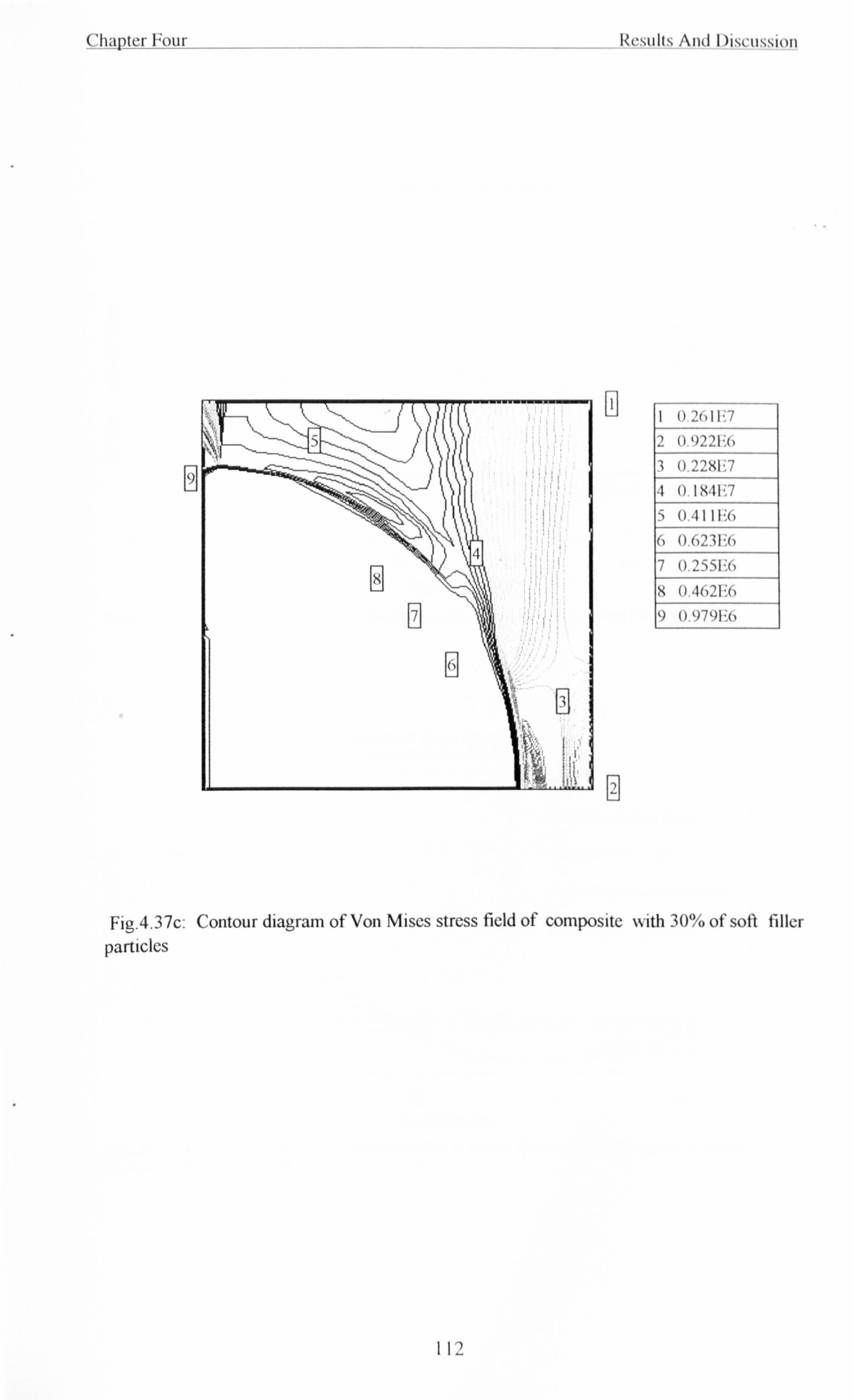
Cfiapter Four IZrmill. ti And I )iu ns`ion
I 0.2611? 7
2 0.9221? (,
3 0.228V17
it 0. I 84V17
ý 0.411I; (,
6 0.6231-', 6 7 0.25S1? 6
8 0.462f; 6 1) 0 1)71)1": (,
L'J
I
Fig. 4.37c: Contour diagram of Von Mises stress field of composite with 30% of soft filler
particles
112
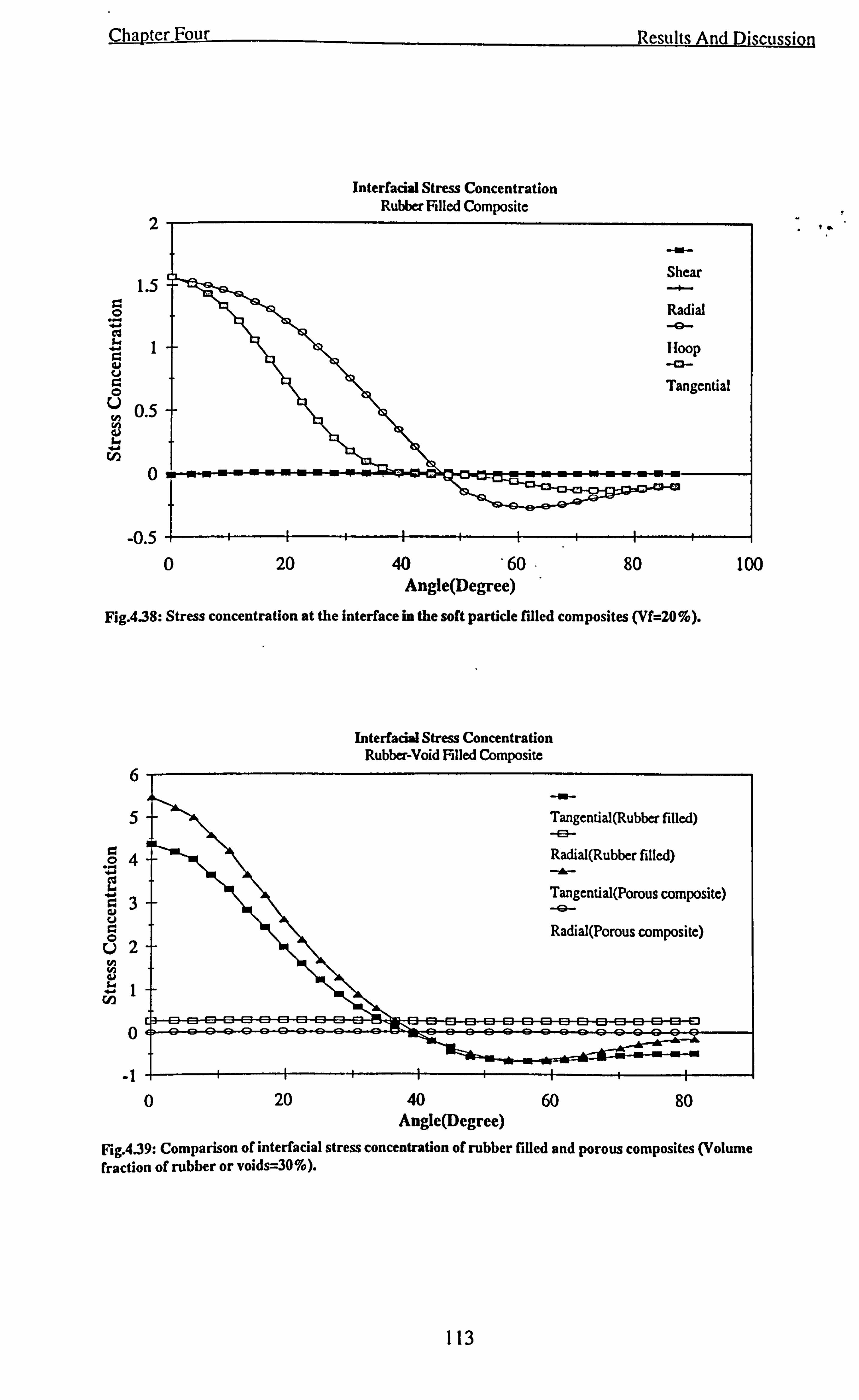
Chapter Four
Interfacial Stress Concentration Rubber Filled Composite
-0.5
Results And Discussion
0 20 40 60 80 Angle(Degree)
Fig. 438: Stress concentration at the interface in the soft particle filled composites (Vf=20%).
Interfacial Stress Concentration Rubber-Void Filled Composite
Tangential(Rubber filled) a
Radial(Rubber filled)
Tangential(Porous composite)
Radial(Porous composite)
0 80 20 40 Angle(Degree)
60
100
Fig. 4.39: Comparison of interfacial stress concentration of rubber filled and porous composites (Volume fraction of rubber or voids=30%).
113
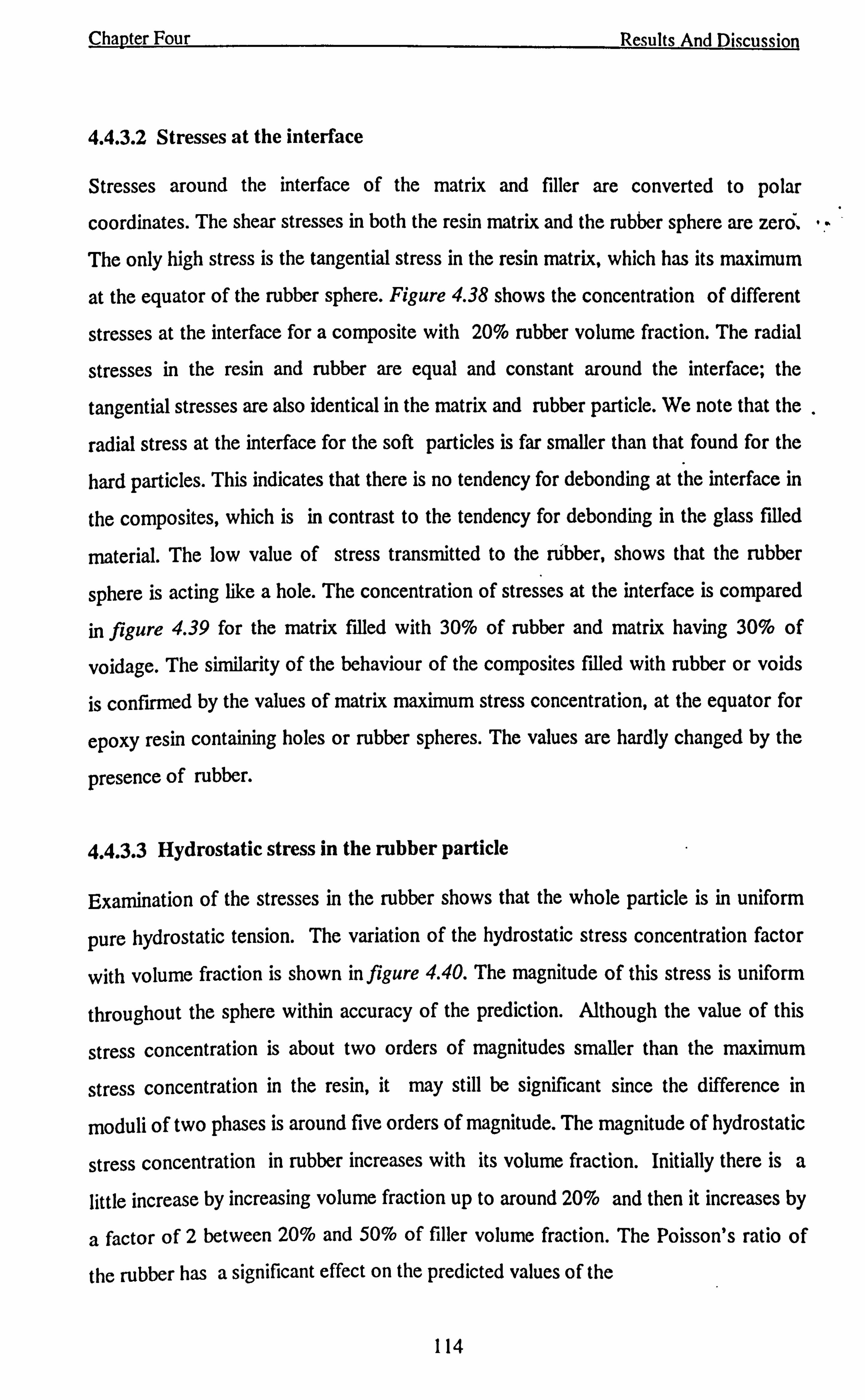
Chapter Four Results And Discussion
4.4.3.2 Stresses at the interface
Stresses around the interface of the matrix and filler are converted to polar
coordinates. The shear stresses in both the resin matrix and the rubber sphere are zero,
The only high stress is the tangential stress in the resin matrix, which has its maximum
at the equator of the rubber sphere. Figure 4.38 shows the concentration of different
stresses at the interface for a composite with 20% rubber volume fraction. The radial
stresses in the resin and rubber are equal and constant around the interface; the
tangential stresses are also identical in the matrix and rubber particle. We note that the
radial stress at the interface for the soft particles is far smaller than that found for the
hard particles. This indicates that there is no tendency for debonding at the interface in
the composites, which is in contrast to the tendency for debonding in the glass filled
material. The low value of stress transmitted to the rubber, shows that the rubber
sphere is acting like a hole. The concentration of stresses at the interface is compared
in figure 4.39 for the matrix filled with 30% of rubber and matrix having 30% of
voidage. The similarity of the behaviour of the composites filled with rubber or voids
is confirmed by the values of matrix maximum stress concentration, at the equator for
epoxy resin containing holes or rubber spheres. The values are hardly changed by the
presence of rubber.
4.4.3.3 Hydrostatic stress in the rubber particle
Examination of the stresses in the rubber shows that the whole particle is in uniform
pure hydrostatic tension. The variation of the hydrostatic stress concentration factor
with volume fraction is shown in figure 4.40. The magnitude of this stress is uniform
throughout the sphere within accuracy of the prediction. Although the value of this
stress concentration is about two orders of magnitudes smaller than the maximum
stress concentration in the resin, it may still be significant since the difference in
moduli of two phases is around five orders of magnitude. The magnitude of hydrostatic
stress concentration in rubber increases with its volume fraction. Initially there is a
little increase by increasing volume fraction up to around 20% and then it increases by
a factor of 2 between 20% and 50% of filler volume fraction. The Poisson's ratio of
the rubber has a significant effect on the predicted values of the
"w
114
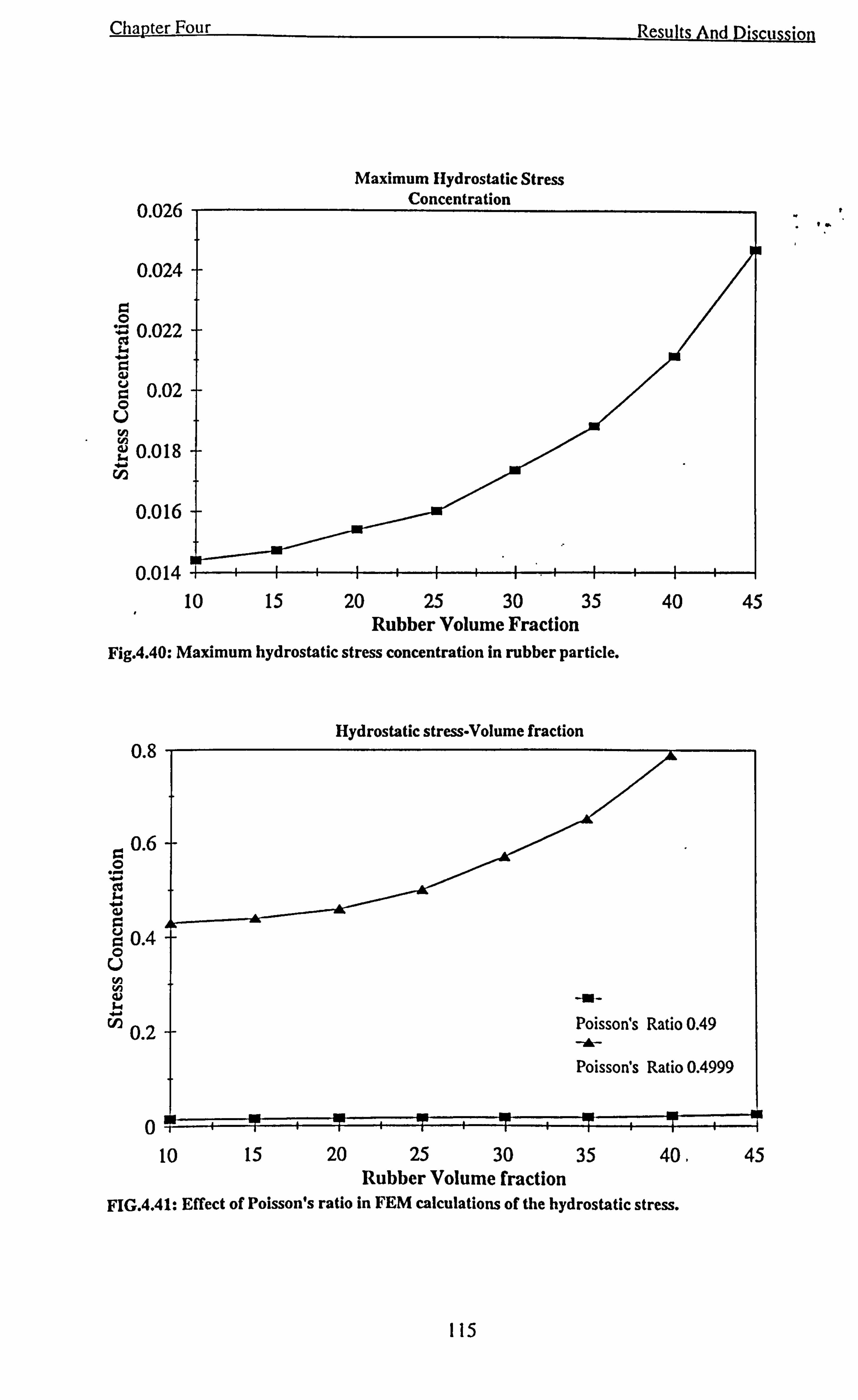
Chapter Four
0.026
0.024
0 ' 0.022 03
0.02 O U W CA WO 0.018f ý Cl)
0.016+
Maximum Hydrostatic Stress Concentration
Results And Discussion
0.0 14 10 15 20 25 30 35 40 45
Rubber Volume Fraction Fig. 4.40: Maximum hydrostatic stress concentration in rubber particle.
0.8
00.6 ...
0.4 0 U W W
rn 0.2
0
Hydrostatic stress-Volume fraction
10 15 20 25 30 35 Rubber Volume fraction
40.
FIG. 4.41: Effect of Poisson's ratio in FEM calculations of the hydrostatic stress.
45
te.
115
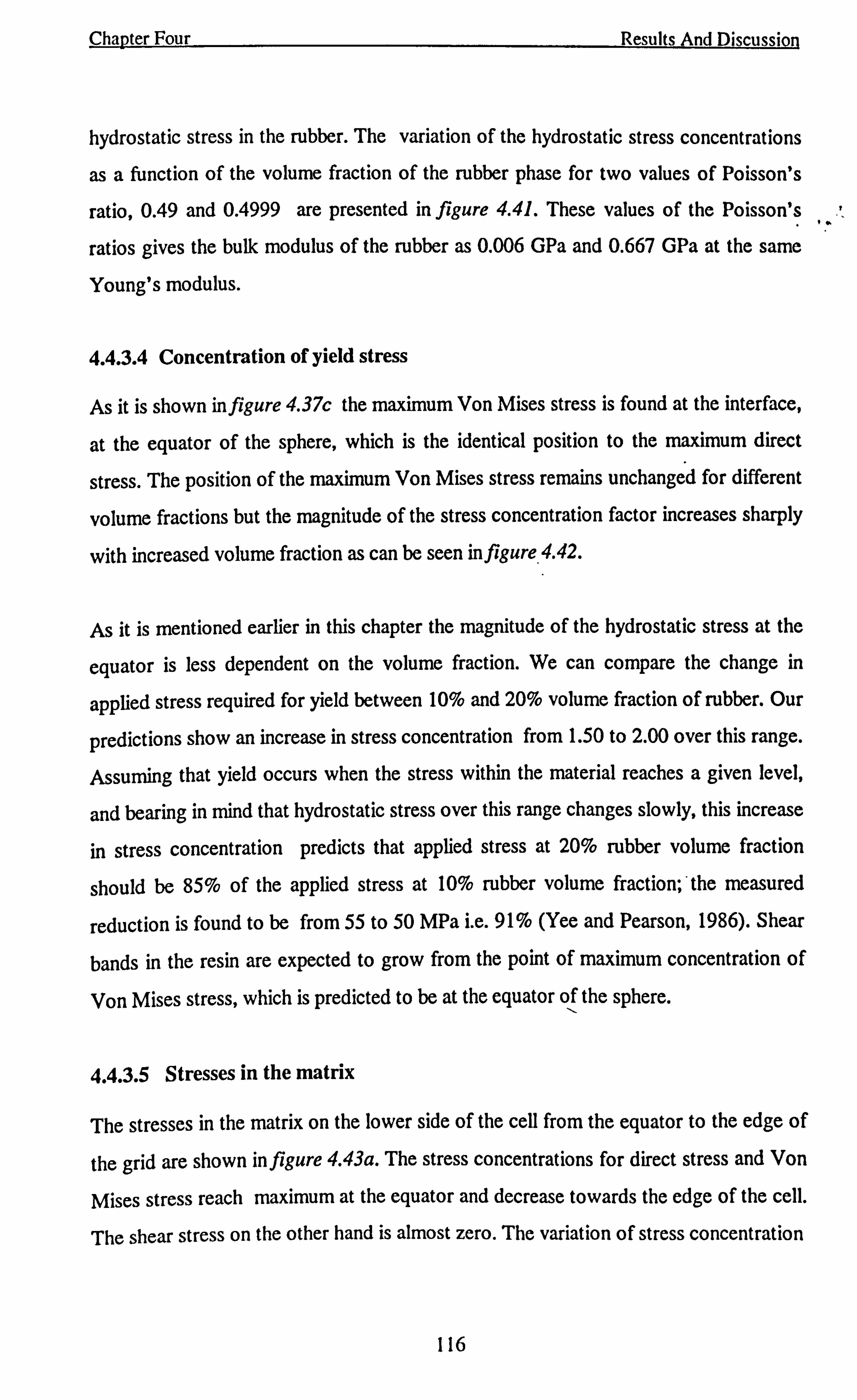
Chapter Four Results And Discussion
hydrostatic stress in the rubber. The variation of the hydrostatic stress concentrations
as a function of the volume fraction of the rubber phase for two values of Poisson's
ratio, 0.49 and 0.4999 are presented in figure 4.41. These values of the Poisson's
ratios gives the bulk modulus of the rubber as 0.006 GPa and 0.667 GPa at the same
Young's modulus.
4.4.3.4 Concentration of yield stress
As it is shown in figure 4.37c the maximum Von Mises stress is found at the interface,
at the equator of the sphere, which is the identical position to the maximum direct
stress. The position of the maximum Von Mises stress remains unchanged for different
volume fractions but the magnitude of the stress concentration factor increases sharply
with increased volume fraction as can be seen in f gure 4.42.
As it is mentioned earlier in this chapter the magnitude of the hydrostatic stress at the
equator is less dependent on the volume fraction. We can compare the change in
applied stress required for yield between 10% and 20% volume fraction of rubber. Our
predictions show an increase in stress concentration from 1.50 to 2.00 over this range.
Assuming that yield occurs when the stress within the material reaches a given level,
and bearing in mind that hydrostatic stress over this range changes slowly, this increase
in stress concentration predicts that applied stress at 20% rubber volume fraction
should be 85% of the applied stress at 10% rubber volume fraction; ' the measured
reduction is found to be from 55 to 50 MPa i. e. 91% (Yee and Pearson, 1986). Shear
bands in the resin are expected to grow from the point of maximum concentration of
Von Mises stress, which is predicted to be at the equator of the sphere.
4.4.3.5 Stresses in the matrix
The stresses in the matrix on the lower side of the cell from the equator to the edge of
the grid are shown in figure 4.43a. The stress concentrations for direct stress and Von
Mises stress reach maximum at the equator and decrease towards the edge of the cell.
The shear stress on the other hand is almost zero. The variation of stress concentration
116
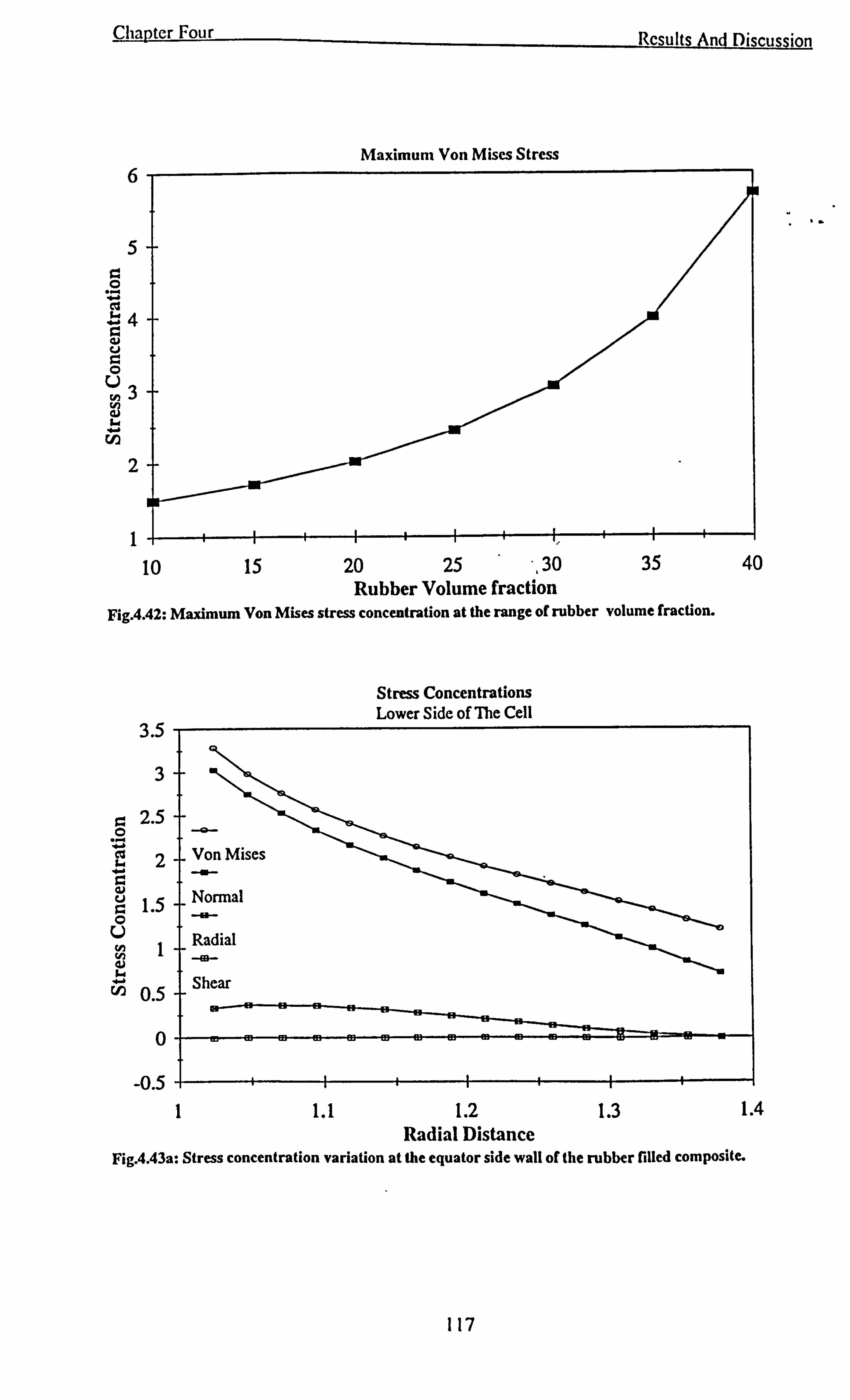
Chapter Four
6
5+
4+
3+
2+
Rcsults And Discussion
Maximum Von Miscs Stress
1 10 15 20 25 -, 30 35 40
Rubber Volume fraction Fig. 4.42: Maximum Von Mises stress concentration at the range of rubber volume fraction.
Stress Concentrations Lower Side of The Cell
3.5
1 4-
o. 5+ -I -ý-
Radial
Shear
0
-o. s 1 1.1 1.2 1.3 1.4
Radial Distance Fig. 4.43a: Stress concentration variation at the equator side wall of the rubber filled composite.
117
Chapter Four Results And Discussion
on the diagonal of the cell follows an opposite trend and decreases from the particle
surface towards the upper right corner edge of the cell, as it can be seen in figure
4.43b.
4.4.4 Fracture behaviour
Two important toughening mechanisms have been identified for the two phase material
under study which consists of a rubbery phase dispersed in a matrix of cross-linked
polymer. The first mechanism is localised shear yielding, or shear banding, which occur
between rubber particles at an angle of approximately 45° to the direction of the
maximum principal tensile stress. Owing to the large number of particles involved, the
volume of thermoset matrix material which can undergo plastic yielding is effectively
increased compared to the single-phase polymer, consequently, far more irreversible
energy dissipation is involved and the toughness of the material is improved. The
second mechanism is internal cavitation or interfacial debonding of the rubbery
particles. The mechanism enables the subsequent growth of the voids formed by plastic
deformation of the epoxy matrix. This irreversible hole-growth in the epoxy matrix in
turn dissipates energy and therefore contributes to the enhancement in the fracture
toughness of the composite.
Gent and Lindley (Gent and Lindley, 1959) have shown that cavitation of rubber can
occur at relatively low stresses. Their analysis was later extended to include surface
energy effects for small holes. Surface energy effects are important for initial holes
smaller than 0.1 µm radius. The hydrostatic stress required for cavitation from an
initial hole with radius greater than about 0.1 µm has been shown to be approximately
close to the modulus of the rubber that is about 0.4 MPa. For an initial hole of radius
0.01 µm the stress required for cavitation increases by a factor of 40.
Internal cavitation of the rubbery particles or debonding of the particles from the
matrix leads to voids (cavities) being formed. By neglecting any plastic void growth at
this stage, the void can be treated as a particle with zero modulus, and a similar
analysis to the one that is described above can therefore be done to calculate the stress
concentration around the voids and the Young's moduli of the voided epoxy polymer.
The formation of voids due to internal cavitation of the rubbery particles or debonding
118
Chapter Four Results And Discussion
of the particles from the matrix does not significantly change the level of the stress
concentration in the epoxy matrix.
The described mechanisms are triggered by the different types of stress concentrations
that act within the overall stress field in the two-phase material. For example, initiation
and growth of the shear bands are largely governed by the concentration of Von Mises
stress in the matrix, whereas cavitation, or interfacial debonding, of the rubber particles
is largely controlled by the hydrostatic (dilatational) tensile stresses. To analyse the
stress field accurately, it is necessary to employ a numerical technique such as the finite
element method.
The yielding of the glassy polymers is usually dependent on the hydrostatic stress
component, and therefore the simple Von Mises criterion is not strictly satisfied.
Instead the Von Mises criterion should be modified as:
Zvm = Ty - µm P (4.13)
where r,,,. is the Von Mises shear stress, as defined in equation 4.14, 'ry is the yield
stress under pure shear, µm is a material constant and P is the hydrostatic stress, Thus
r
L(QI-Q2) 2+ (o'2-Q3)2 + (Q3-61)2
=2 Qvm2 =6 zvm2 (4.14)
and
P= 3(o'I
+(7s+Q3) (4.15)
where a,,,,, is the Von Mises tensile stress and the value of µm has been reported to be
between 0.175 and 0.225. In this study this value is taken to be 0.2. It is obvious from
equation 4.13 that the stress required for the material to shear yield under tensile
loading is reduced compared to the prediction of the unmodified Von Mises criteria.
Hence, the relative size of the plastic zone will be increased. The tensile strength of the
rubber toughened epoxy is shown in figure 4.44.
119
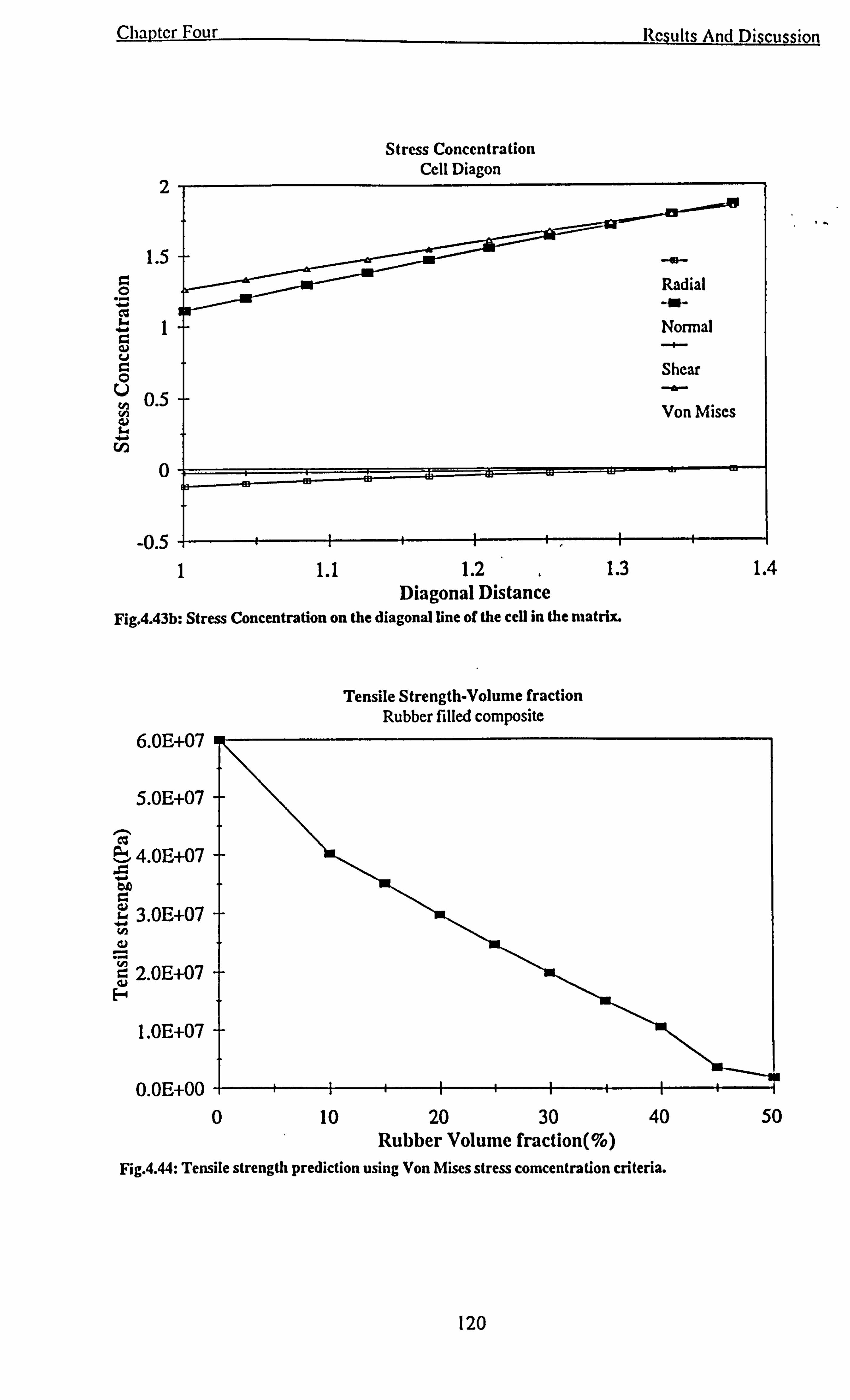
Chapter Four
Stress Concentration Cell Diagon
2
o. 5+
0
-0. s 1 1.1 1.2 1.3
Diagonal Distance Fig. 4.43b: Stress Concentration on the diagonal line of the cell in the matrix.
Tensile Strength-Volume fraction Rubber filled composite
6.0E+07
5.0E+07
. -. cC a: ' 4.0E+07
00 ý 3.0E+07
2.0E+07 H
1.0E+07
Results And Discussion
--«- Shear
Von Mises
0.0E+00 0 10 20 30 40
Rubber Volume fraction(%) Fig. 4.44: Tensile strength prediction using Von Mises stress comcentration criteria.
1.4
50
120
Chanter Four Results And Discussion
Schwier et al (Schwier et al , 1985) in their experimental investigation of polystyrene filled with polybutadiene rubber spheres, concluded that intrinsic cavitation of rubber
spheres occurred at about an overall hydrostatic tension of 60 MPa.
Our results predict that for 20% volume fraction of rubber the concentration factor of hydrostatic tension in the rubber is about 0.025. Shear band formation probably occurs
at about 30 MPa stress for epoxy resins. Keeping the average applied tensile stress at
this level would subject the rubber spheres to a further 1 MPa hydrostatic tension.
Cavitation of rubber particles on fracture surfaces is generally found to start from the
centre of the sphere. Our predictions do not indicate a preferred point of initiation but
clearly show that the imposition of an overall tensile stress of the order of the matrix
yield stress places the rubber particles in sufficient hydrostatic tension to initiate
cavitations from small flaws. These flaws may be areas of rubber which are not fully
polymerised and cannot be observed by conventional microscopic techniques. There is
some argument as to whether or not the cavitation of the rubber particles is necessary
for shear bands to form. The exact stress levels for shear band formation and cavitation
will depend on the values of stress required to form matrix shear bands and cause
rubber cavitation for the system under study.
Epoxy resin reinforced with rubber spheres may be described as an inherently tough
material since the position of maximum stress concentration, where a crack would be
likely to develop, is at the equator of the sphere. The sphere acts as a barrier to any
further growth of the crack. However, the maximum stress concentration rise sharply
at high volume fractions. A simple description of toughness could be that yield is the
preferred mechanism to the growth of the crack. Considering the very high stress
concentration of applied stress at high volume fraction, crack growth could become
more dominant at high volume fractions leading to the decreased toughness of
composites filled with rubber particles. This effect was noted by Kunz (Kunz et al,
1982) who found a rapid increase in toughness until around 5 pbw (parts by weight)
rubber, around 10% volume fraction, followed by a plateau. A similar effect is found
by Spanoudakis and Young (Spanoudakis and Young, 1984) for epoxy resin reinforced
with glass spheres treated with a release agent; the sphere must be behaving as a stable
hole, and stress distribution in the resin must be similar to our prediction here; the
I. r
121
Chapter Four Results And Discussion
observed crack growth for glass spheres treated with a release agent supported the
expected maximum stress concentration at the equator of the sphere. They found that
fracture toughness decreased with volume fraction above 30% for this material. Although for glass spheres coupled to the resin matrix the toughness increased
throughout the range of filler volume fraction.
Stress distribution in the matrix for resin containing rubber spheres has been found to
be very similar to that of a resin containing holes. Shear band formation in the resin
would occur in a similar way for the two materials. However, epoxy resin containing
holes is known to be a very poor material. We therefore can postulate that shear band
formation is not the only important fracture mechanism for this material. Our results
have shown that cavitation of the rubber particles is likely to occur, in agreement with
experimental observations; after cavitation the rubber may be stretched. It appears that
the process of rubber cavitation and stretching may make important contributions to
the overall fracture energy. The magnitude of these contributions is dependent on the
modulus of the rubber. Further contributions to the fracture energy of epoxy resin
containing rubber spheres may arise from the physical presence of the rubber which
would act as a crack stopper to a growing crack attracted to the equator of the sphere
by either the concentration of direct stress or the initiation of shear bands.
122
Chapter Four Results And Discussion
4.5 FIBRE REINFORCED COMPOSITES
In this section the response of epoxy resin reinforced with glass fibres to transverse
tensile and shear loading is studied. The physical properties of the epoxy resin and
glass fibres are presented in table 4.1.
4.5.1 Transverse tensile loading
4.5.1.1 Modulus
A tensile loading in the transverse direction of the fibres is applied to the composite.
The modulus of particulate filled composites is compared with the moduli of transverse
and longitudinal fibre reinforced composite having the same constituents in figure 4.6.
As expected the longitudinal modulus of the fibre composite is much higher than that
of the particulate composite, while the transverse modulus is lower. Maximum volume
fractions of the fibres are 0.785 and 0.907 for square array and hexagonal array,
respectively. These values reduce to 0.57 and 0.74 for square and hexagonal array in
particulate composites. Therefore a higher volume fraction and modulus can be
reached in fibre composites.
It is observed that the addition of fibres produces a substantial increase in the
transverse modulus of the binder material; however, the effect of an increase in fibre
modulus is a gradually diminishing one becoming asymptotic to the value obtained for
the infinitely rigid fibre. Therefore, at high values of the fibre modulus, The ratio of
transverse Young's modulus to longitudinal Young's modulus becomes relatively small
which is one of the significant structural problems associated with the use of high
modulus filaments in composite structures. If multiple oriented fibre arrays are
utilised to solve the problem of low stiffness in the transverse direction, a decrease in
the major stiffness of the fibrous composite follows.
4.5.1.2 Concentration of applied stress
Contours of the direct stress and Von Mises stress are obtained for fibre reinforced
composites as shown in figures 4.45a-b. These contour diagrams indicate that the
123
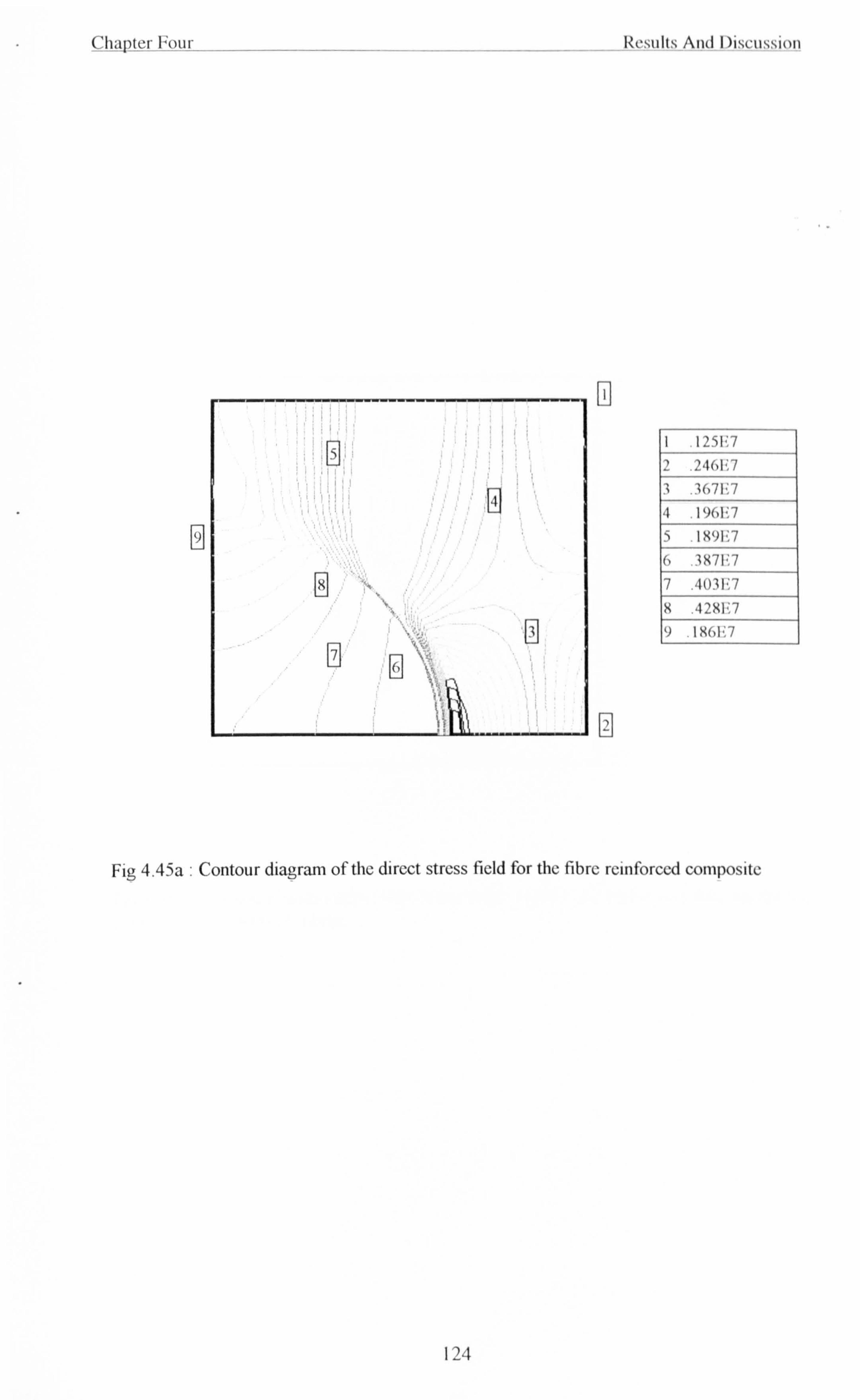
Chapter Four
F)
IZrsu(s And I )iscussi<m
L2
I I 25I17
' 246117
Z . 367117
4 . 196117
ý .1
x9F. 7
6 387117
7 . 403117
8 . 428I17
9
. 186I": 7
Fig 4.45a : Contour diagram of the direct stress field for the fibre reinforced composite
124
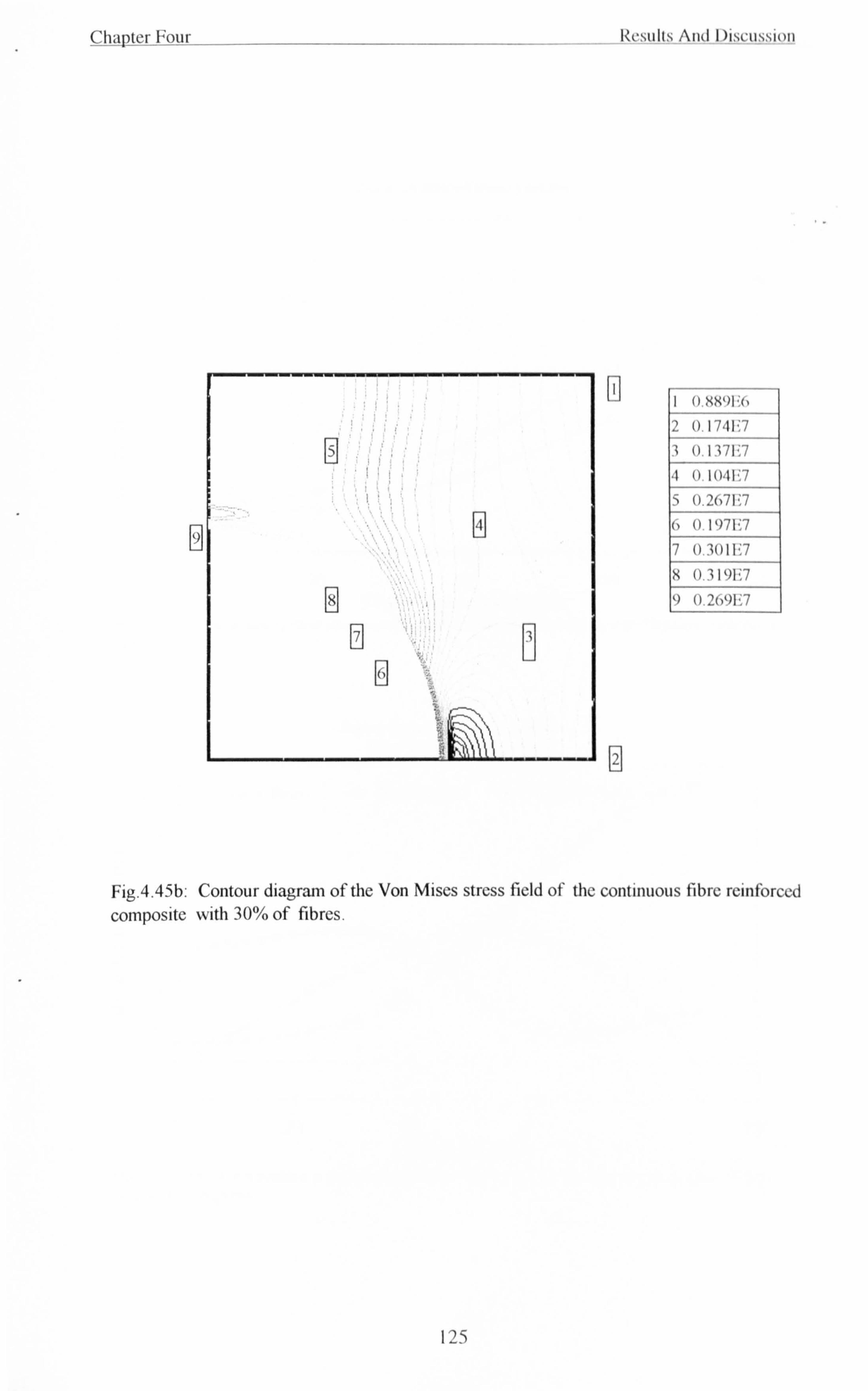
ChapterFour Results And Discussion
9
F
ýý
{6 1 0.889F6 20 1741? 7
3 U1371`. 7
"1 n_ I(141-'17
5 U. 2(, 71; 7
() 0 1971; 7
7 03011`17
(1.3191: 7 8 1) ()
. 201? 7
Fig. 4.45b: Contour diagram of the Von Mises stress field of the continuous fibre reinforced composite with 30% of fibres.
125
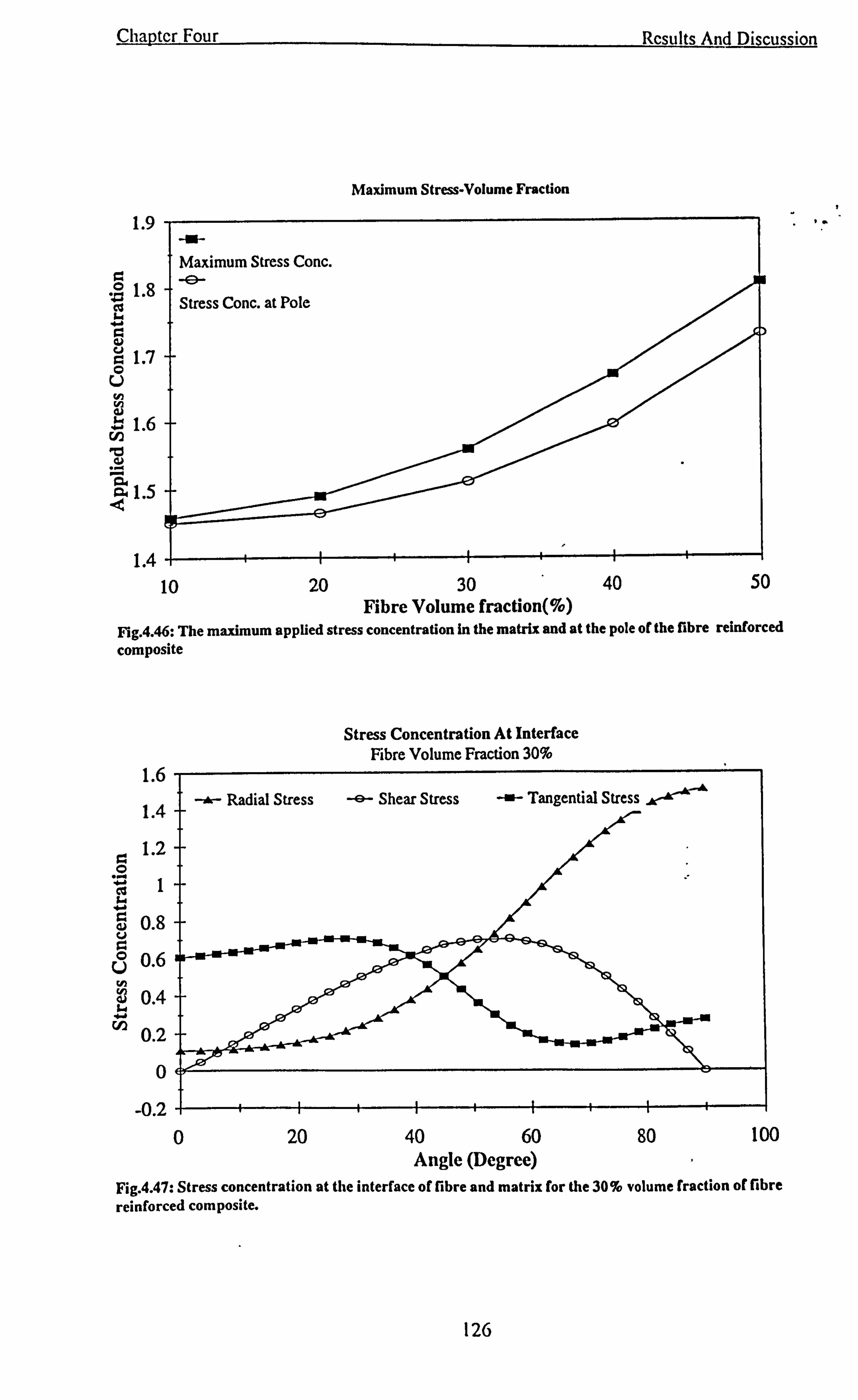
Chapter Four
Maximum Stress-Volume Fraction
1.9
U H wl v N cn
.., -
Maximum Stress Conc.
1.8 -e- Stress Conc. at Pole
1.7
1.6
1.4+ 10
f -i- 20
{ III 30 40 50
Fibre Volume fraction(%) Fig. 4.46: The maximum applied stress concentration in the matrix and at the pole of the fibre reinforced composite
Stress Concentration At Interface Fibre Volume Fraction 30%
0 20 40 60 Angle (Degree)
Rcsults And Discussion
4
80 100
Fig. 4.47: Stress concentration at the interface of fibre and matrix for the 30% volume fraction of fibre
reinforced composite.
126
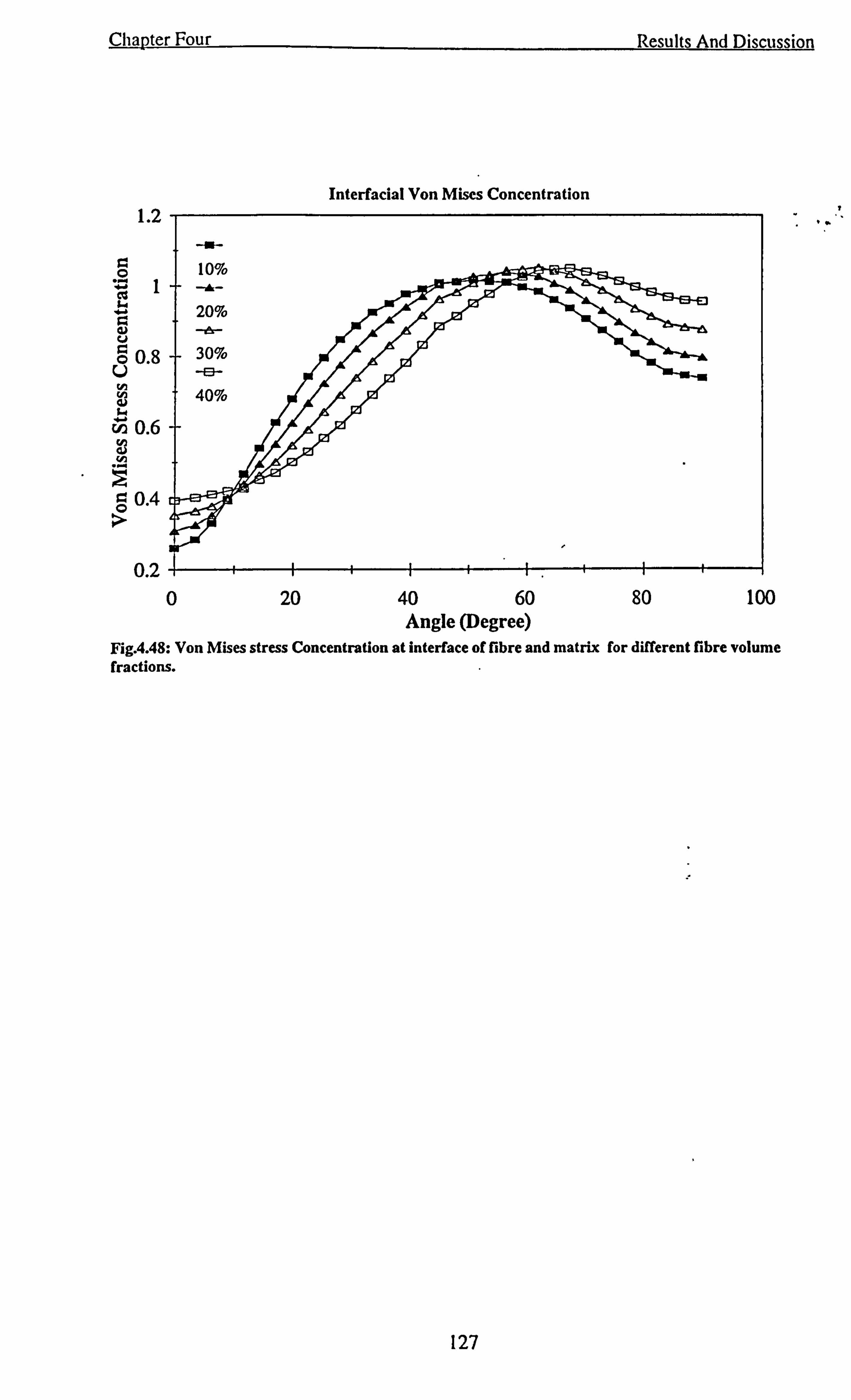
Chapter Four
1.2
0.2 4 0 20
Results And Discussion
Interfacial Von Mises Concentration
40 60 80 100 Angle (Degree)
Fig. 4.48: Von Mises stress Concentration at interface of fibre and matrix for different fibre volume fractions.
127
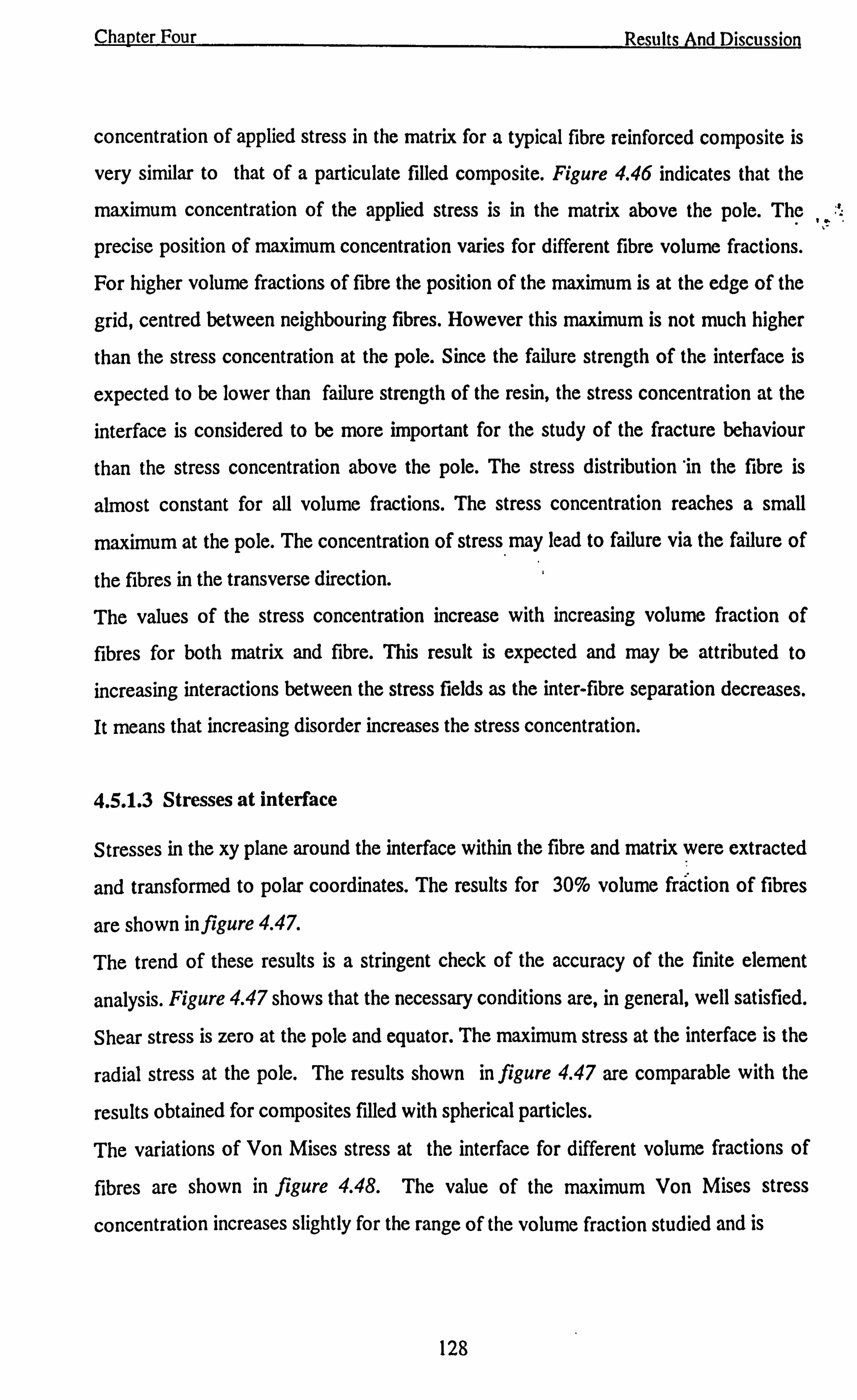
Chapter Four Results And Discussion
concentration of applied stress in the matrix for a typical fibre reinforced composite is
very similar to that of a particulate filled composite. Figure 4.46 indicates that the
maximum concentration of the applied stress is in the matrix above the pole. The
precise position of maximum concentration varies for different fibre volume fractions.
For higher volume fractions of fibre the position of the maximum is at the edge of the
grid, centred between neighbouring fibres. However this maximum is not much higher
than the stress concentration at the pole. Since the failure strength of the interface is
expected to be lower than failure strength of the resin, the stress concentration at the
interface is considered to be more important for the study of the fracture behaviour
than the stress concentration above the pole. The stress distribution 'in the fibre is
almost constant for all volume fractions. The stress concentration reaches a small
maximum at the pole. The concentration of stress may lead to failure via the failure of
the fibres in the transverse direction.
The values of the stress concentration increase with increasing volume fraction of
fibres for both matrix and fibre. This result is expected and may be attributed to
increasing interactions between the stress fields as the inter-fibre separation decreases.
It means that increasing disorder increases the stress concentration.
4.5.1.3 Stresses at interface
Stresses in the xy plane around the interface within the fibre and matrix were extracted
and transformed to polar coordinates. The results for 30% volume fraction of fibres
are shown in figure 4.47.
The trend of these results is a stringent check of the accuracy of the finite element
analysis. Figure 4.47 shows that the necessary conditions are, in general, well satisfied.
Shear stress is zero at the pole and equator. The maximum stress at the interface is the
radial stress at the pole. The results shown in figure 4.47 are comparable with the
results obtained for composites filled with spherical particles.
The variations of Von Mises stress at the interface for different volume fractions of
fibres are shown in figure 4.48. The value of the maximum Von Mises stress
concentration increases slightly for the range of the volume fraction studied and is
128
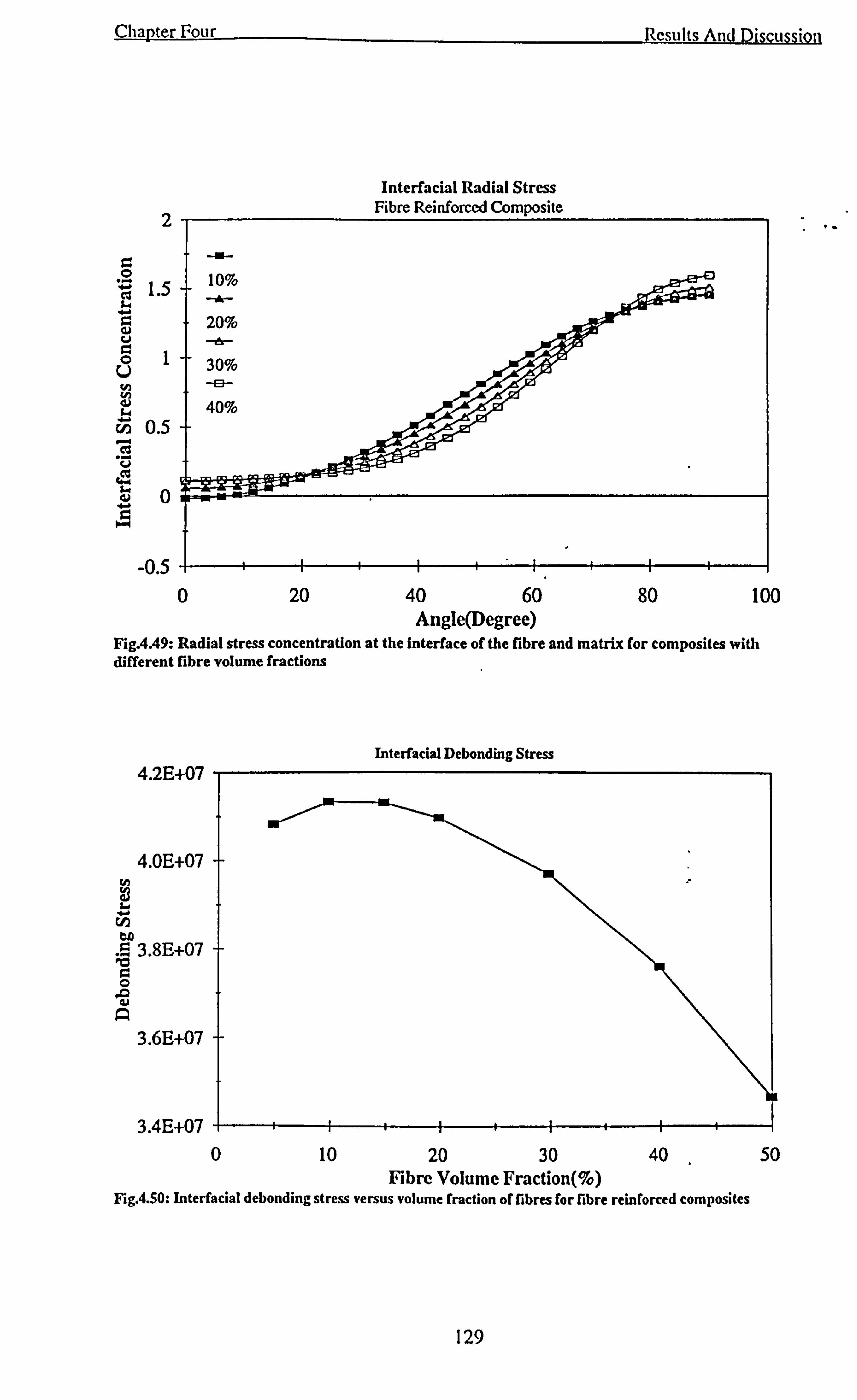
Chapter Four Results And Discussion
Interfacial Radial Stress Fibre Reinforced Composite
I.
0.5
r--I II1I _0.5
0 20 40 60 80 Angle(Degree)
100
Fig. 4.49: Radial stress concentration at the interface of the fibre and matrix for composites with different fibre volume fractions
4.2E+07
4.0E+07
ir r-+ ý
on 3.8E+07
0
A 3.6E+07
3.4E+07
Interfacial Debonding Stress
0 10 20 30 40 50 Fibre Volume Fraction(%)
Fig. 4. S0: Interfacial debonding stress versus volume fraction of fibres for fibre reinforced composites
129
Chapter Four Results And Discussion
almost constant. However, the position of the maximum at the interface moves from
about 40° at low volume fraction towards the pole for the higher volume fractions.
4.5.1.4 Fracture strength
The overall stress distribution for the matrix and fibre may be used to deduce the
failure mechanisms of this type of composites. It is assumed that failure is essentially
brittle, and takes place when local stress reaches a critical level. The concentration of
the stress in the fibre may lead to failure via transverse splitting of the fibres. The
concentration of applied stress in the radial direction at the interface may lead to tensile
failure of the interface. The radial stress variations at the interface are shown for
different volume fractions in figure 4.49. The position of the maximum is at the pole
over the range of the volume fraction. The increasing values of stress concentration
with volume fraction imply a reduction in overall applied stress required for failure.
Thus the fracture strength of the material is predicted to fall with increasing fibre
volume fraction. Although the rise of the maximum stress concentration is relatively
slow.
The transverse strength of the glass fibres is about 2758 MPa which is much higher
than that of the epoxy resin which is about 60 MPa (Gibson, 1994). Since the
concentration of applied stress at the pole is the same in the fibre and the matrix at the
interface, failure is predicted to occur at the interface at the pole via- failure of the
matrix. Assuming the strength of the interface equals the strength of the resin (i. e.
assuming good bonding), the overall applied stress for which the interface failure is
expected can be calculated from the concentration of the radial stress at the pole.
The initiation of a fibre/matrix debond is analysed using an interfacial failure criterion,
proposed by Sun and Zhou (Sun and Zhou, 1988) for free edge delamination of
composite laminates, which here is modified to accommodate the cylindrical geometry
of the fibre matrix interface,
22 Cr Tre
I- 1+ - =1 RS (4.16)
ýw
130
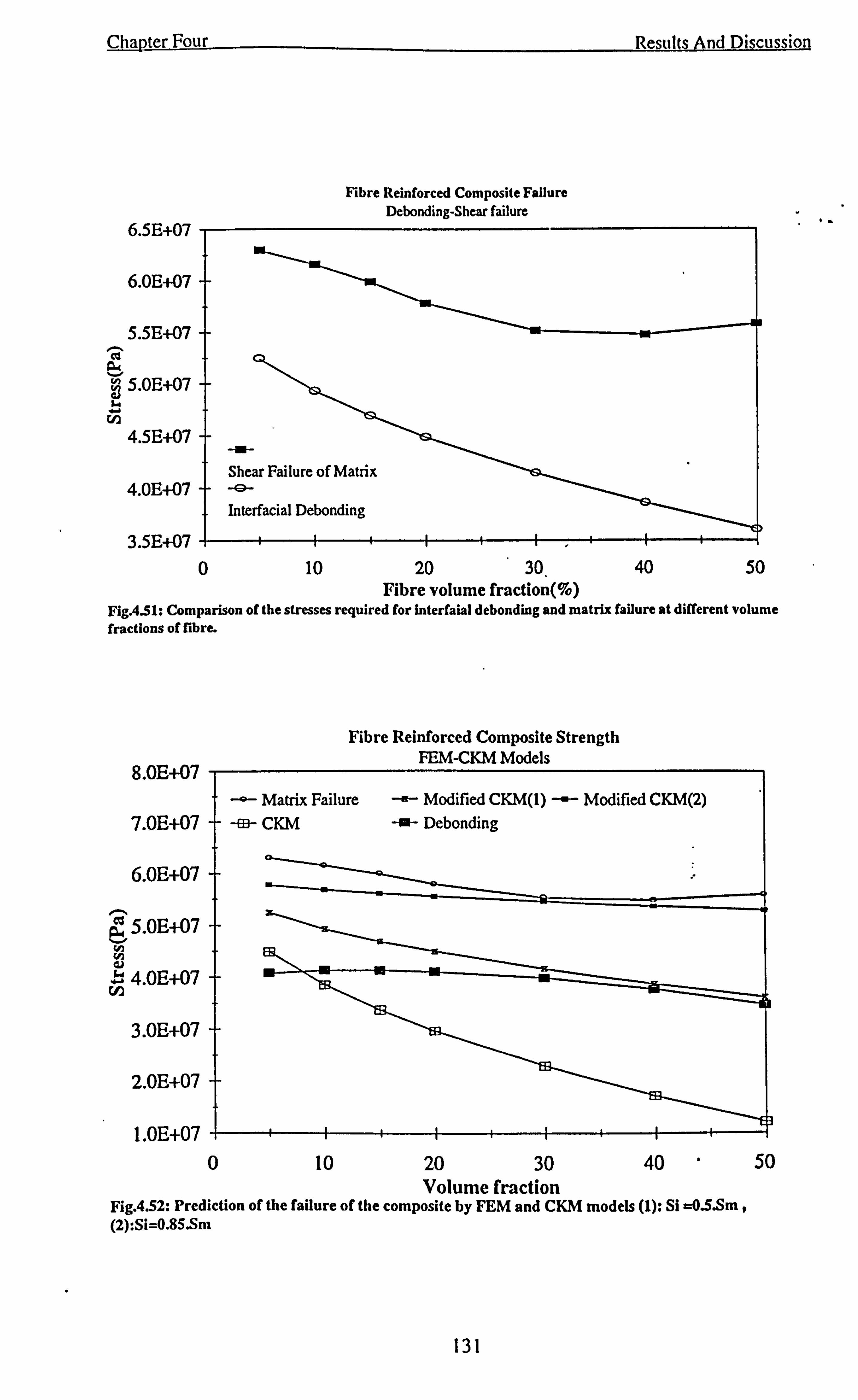
Chapter Four
6.5E+07
6.0E+07
5.5E+07
Fibre Reinforced Composite Failure Debonding-Shear failure
3.5E+07 I-ý ý-1 i--4 0 10 20 30
ý
Results And Discussion
40
4
50 Fibre volume fraction(%)
Fig. 451: Comparison of the stresses required for interfaial debonding and matrix failure at different volume fractions of fibre.
Fibre Reinforced Composite Strength FEM-CKM Models
8.0E+07 Matrix Failure -- Modified CKM(1) -- Modified CKM(2)
7.0E+07 -s- CKM -- Debonding
6.0E+07
S. OE+07
rA Q *'a 4.0E+07 W
3.0E+07
2.0E+07 -F
1.0E+07 0 10 20 30
Volume fraction
4
40 50
Fig. 4.52: Prediction of the failure of the composite by FEM and CKM models (1): Si =0.5. Sm , (2): Si=0.85. Sm
131
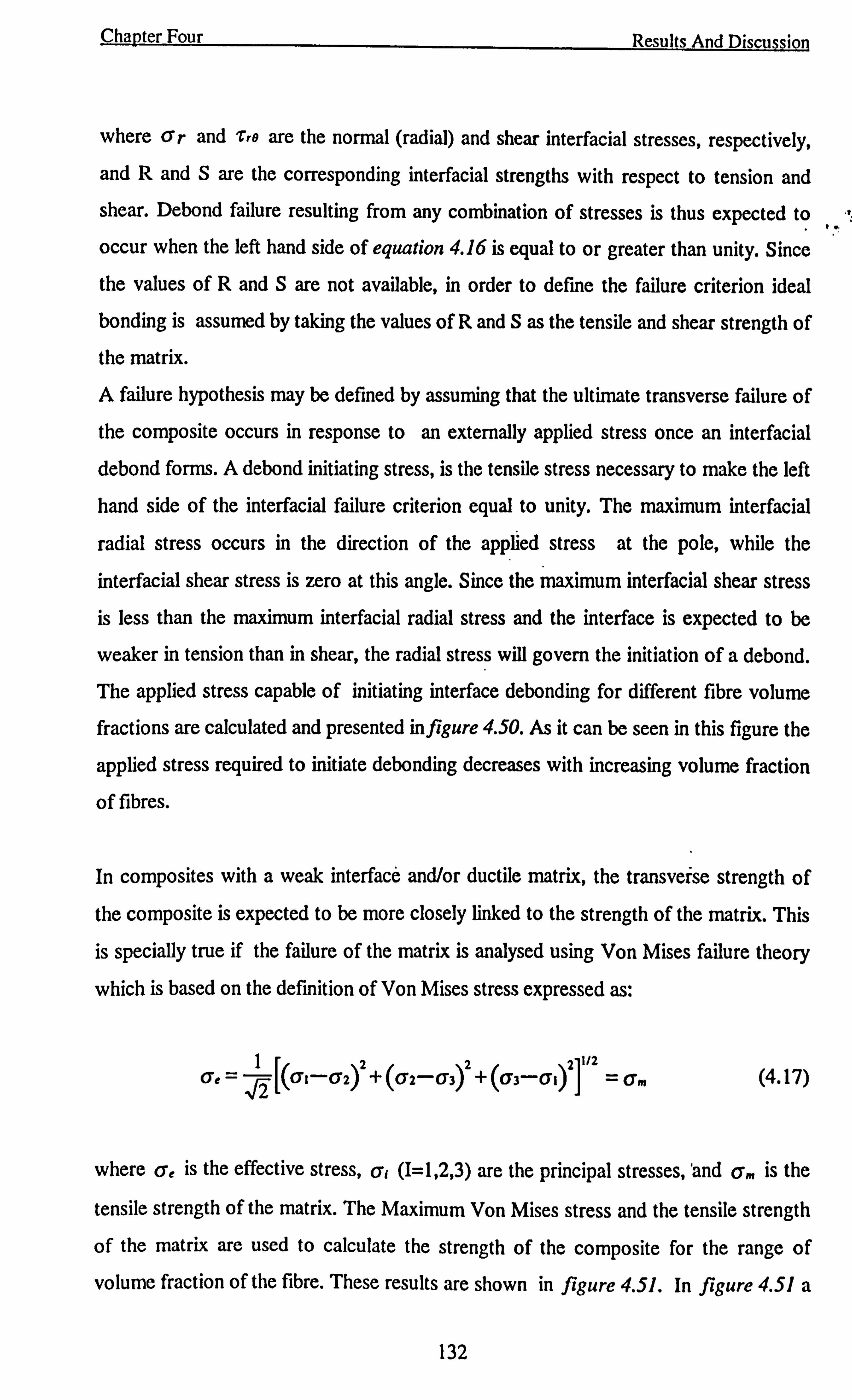
Chanter Four Results And Discussion
where Cyr and rro are the normal (radial) and shear interfacial stresses, respectively,
and R and S are the corresponding interfacial strengths with respect to tension and
shear. Debond failure resulting from any combination of stresses is thus expected to
occur when the left hand side of equation 4.16 is equal to or greater than unity. Since
the values of R and S are not available, in order to define the failure criterion ideal
bonding is assumed by taking the values of R and S as the tensile and shear strength of
the matrix.
A failure hypothesis may be defined by assuming that the ultimate transverse failure of
the composite occurs in response to an externally applied stress once an interfacial
debond forms. A debond initiating stress, is the tensile stress necessary to make the left
hand side of the interfacial failure criterion equal to unity. The maximum interfacial
radial stress occurs in the direction of the applied stress at the pole, while the
interfacial shear stress is zero at this angle. Since the maximum interfacial shear stress
is less than the maximum interfacial radial stress and the interface is expected to be
weaker in tension than in shear, the radial stress will govern the initiation of a debond.
The applied stress capable of initiating interface debonding for different fibre volume
fractions are calculated and presented in figure 4.50. As it can be seen in this figure the
applied stress required to initiate debonding decreases with increasing volume fraction
of fibres.
In composites with a weak interface and/or ductile matrix, the transverse strength of
the composite is expected to be more closely linked to the strength of the matrix. This
is specially true if the failure of the matrix is analysed using Von Mises failure theory
which is based on the definition of Von Mises stress expressed as:
11/2 6c = r-
[(QI-62)2 + (Q2-Q3)2 + (O'3-0ý1)2J
= Qm (4.17)
where a is the effective stress, a, (1=1,2,3) are the principal stresses, 'and am is the
tensile strength of the matrix. The Maximum Von Mises stress and the tensile strength
of the matrix are used to calculate the strength of the composite for the range of
volume fraction of the fibre. These results are shown in figure 4.51. In figure 4.51 a
132
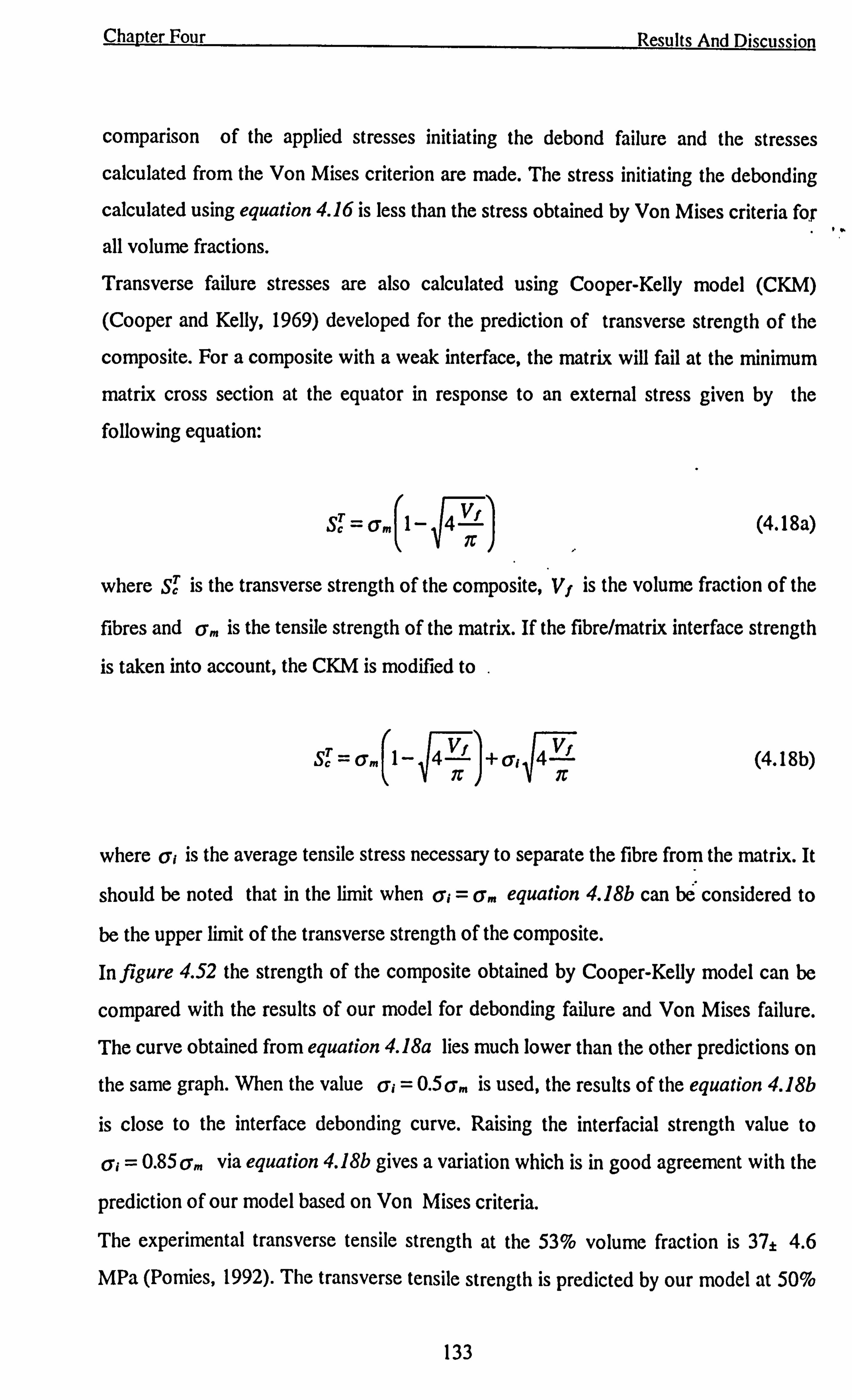
Chanter Four Results And Discussion
comparison of the applied stresses initiating the debond failure and the stresses
calculated from the Von Mises criterion are made. The stress initiating the debonding
calculated using equation 4.16 is less than the stress obtained by Von Mises criteria fo,;
all volume fractions.
Transverse failure stresses are also calculated using Cooper-Kelly model (CKM)
(Cooper and Kelly, 1969) developed for the prediction of transverse strength of the
composite. For a composite with a weak interface, the matrix will fail at the minimum
matrix cross section at the equator in response to an external stress given by the
following equation:
. Sc = vm 1- 4VI
n (4.18a)
I
where SC is the transverse strength of the composite, Vf is the volume fraction of the
fibres and am is the tensile strength of the matrix. If the fibre/matrix interface strength
is taken into account, the CKM is modified to .
ST =Qm 1- 4Vt +O'r 4V ný
(4.18b)
where a, is the average tensile stress necessary to separate the fibre from the matrix. It
should be noted that in the limit when a, = am equation 4.18b can be considered to
be the upper limit of the transverse strength of the composite.
In figure 4.52 the strength of the composite obtained by Cooper-Kelly model can be
compared with the results of our model for debonding failure and Von Mises failure.
The curve obtained from equation 4.18a lies much lower than the other predictions on
the same graph. When the value a, = 0.5 am is used, the results of the equation 4.18b
is close to the interface debonding curve. Raising the interfacial strength value to
a, = 0.85 am via equation 4.18b gives a variation which is in good agreement with the
prediction of our model based on Von Mises criteria.
The experimental transverse tensile strength at the 53% volume fraction is 37± 4.6
MPa (Pomies, 1992). The transverse tensile strength is predicted by our model at 50%
133
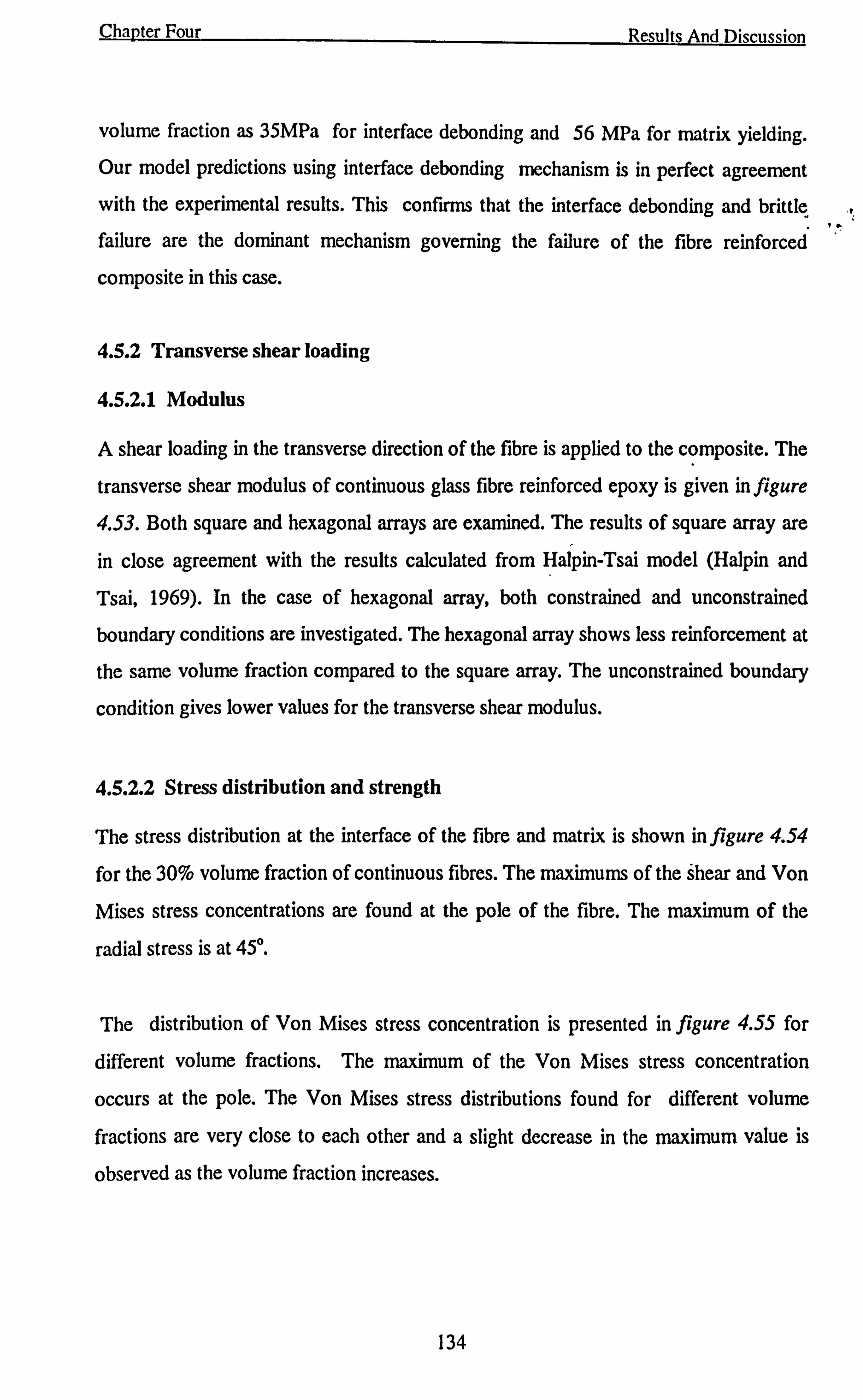
Chapter Four Results And Discussion
volume fraction as 35MPa for interface debonding and 56 MPa for matrix yielding. Our model predictions using interface debonding mechanism is in perfect agreement
with the experimental results. This confirms that the interface debonding and brittle
failure are the dominant mechanism governing the failure of the fibre reinforced
composite in this case.
4.5.2 Transverse shear loading
4.5.2.1 Modulus
A shear loading in the transverse direction of the fibre is applied to the composite. The
transverse shear modulus of continuous glass fibre reinforced epoxy is given in figure
4.53. Both square and hexagonal arrays are examined. The results of square array are
in close agreement with the results calculated from Halpin-Tsai model (Halpin and
Tsai, 1969). In the case of hexagonal array, both constrained and unconstrained
boundary conditions are investigated. The hexagonal array shows less reinforcement at
the same volume fraction compared to the square array. The unconstrained boundary
condition gives lower values for the transverse shear modulus.
4.5.2.2 Stress distribution and strength
The stress distribution at the interface of the fibre and matrix is shown in figure 4.54
for the 30% volume fraction of continuous fibres. The maximums of the shear and Von
Mises stress concentrations are found at the pole of the fibre. The maximum of the
radial stress is at 45°.
The distribution of Von Mises stress concentration is presented in figure 4.55 for
different volume fractions. The maximum of the Von Mises stress concentration
occurs at the pole. The Von Mises stress distributions found for different volume
fractions are very close to each other and a slight decrease in the maximum value is
observed as the volume fraction increases.
134
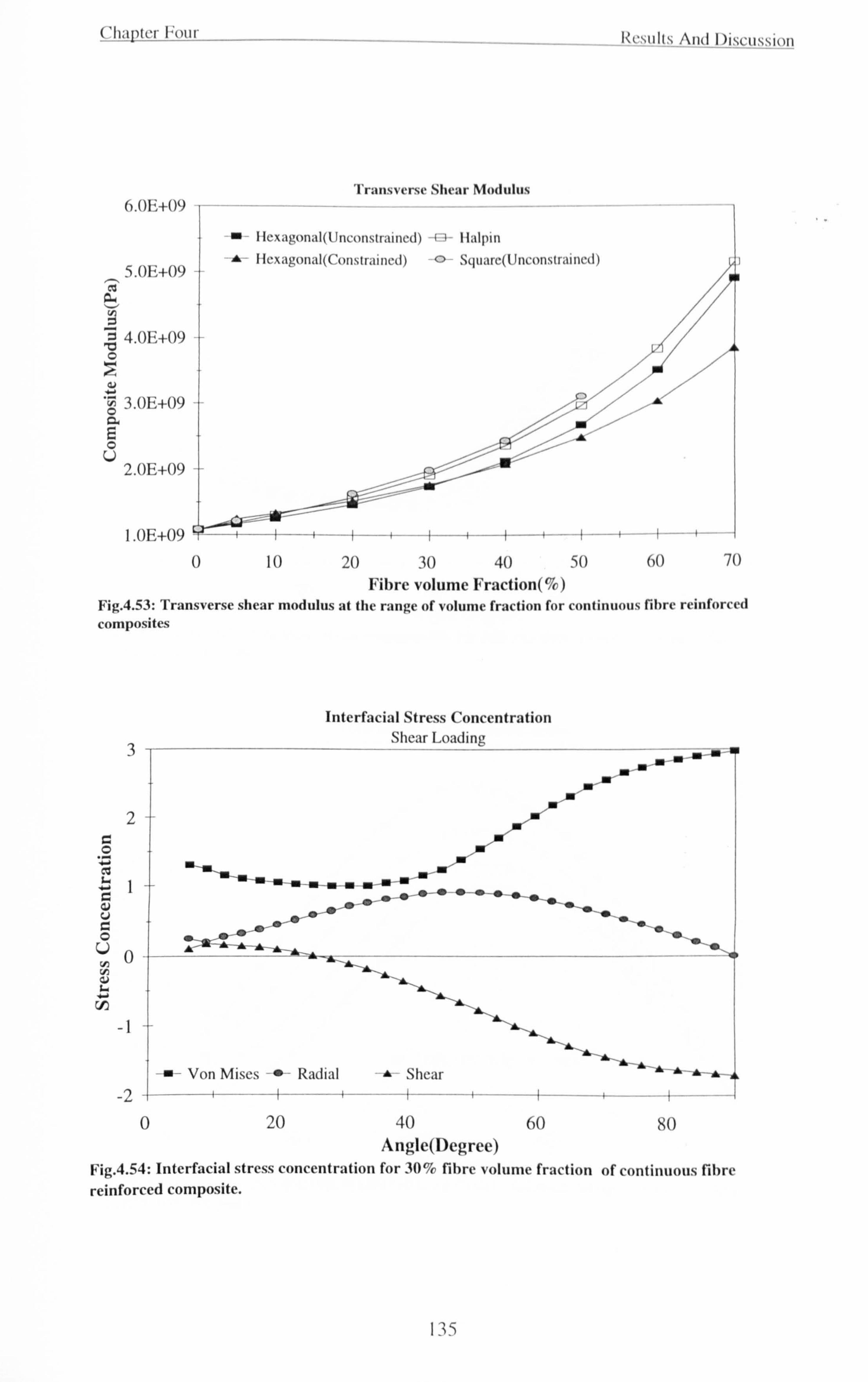
Chapter Four
6. OE+09
5.0E+09
.. ý ý 4.0E+09 -
ö 3.0E+09
2.0E+09 -
0
Transverse Shear Modulus
m Ilcxagonal(Unconstraincd) ta- Halpin
+I Icxagonal(Constraincd) o Syuarc(Unconstraincd)
10 70
Fig. 4.53: Transverse shear modulus at the range of volume fraction for continuous fibre reinforced composites
3,
2+
I
o -+-
I+
Interfacial Stress Concentration Shear Loading
I: rýullý And I)i. tirii. ti. mun
20 30 40 50 60 Fibre volume Fraction(%)
_ ý-ý-ý-a-ýý-+- ý-ýý -ý-tr ; -i-s--
"-o'° 4w-
Von Mises -f- Radial Shear
--4-
0 20 40 60 Angle(Degree)
to
-. -" _i
80
Fig. 4.54: Interfacial stress concentration for 30% fibre volume fraction of continuous fibre
reinforced composite.
135
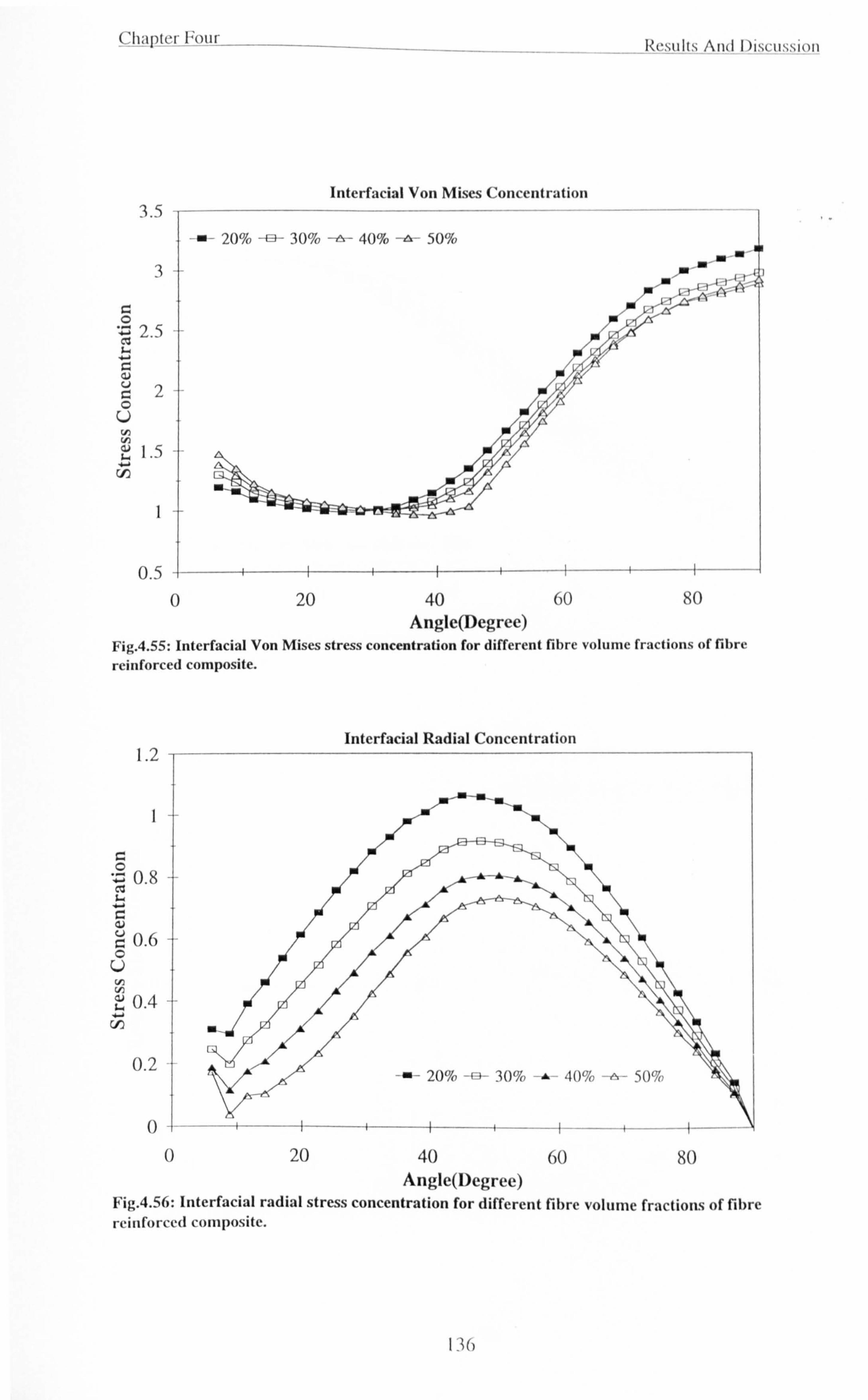
Chapter Four
3.5 - Interfacial Von Mises Concentration
-- 20% -- 30% -- 40% -- 50%
3
ý C ý 2.5 1. ý a v ý2 0
U Cl) C')
1.5 4. cn
I
0.5 0 20 40 60
Angle(Degree)
Results And Discussion
80
Fig. 4.55: Interfacial Von Mises stress concentration for different fibre volume fractions of fibre
reinforced composite.
1.2
I= 0.8 -
0.6
U
"; 0.4 cdo
0.2
Interfacial Radial Concentration
0+ýý --ý-- F----+ _{ --- +_ - _--I- - 0 20 40 60 80
Angle(Degree) Fig. 4.56: Interfacial radial stress concentration for different fibre volume fractions of fibre
reinforced composite.
1 36
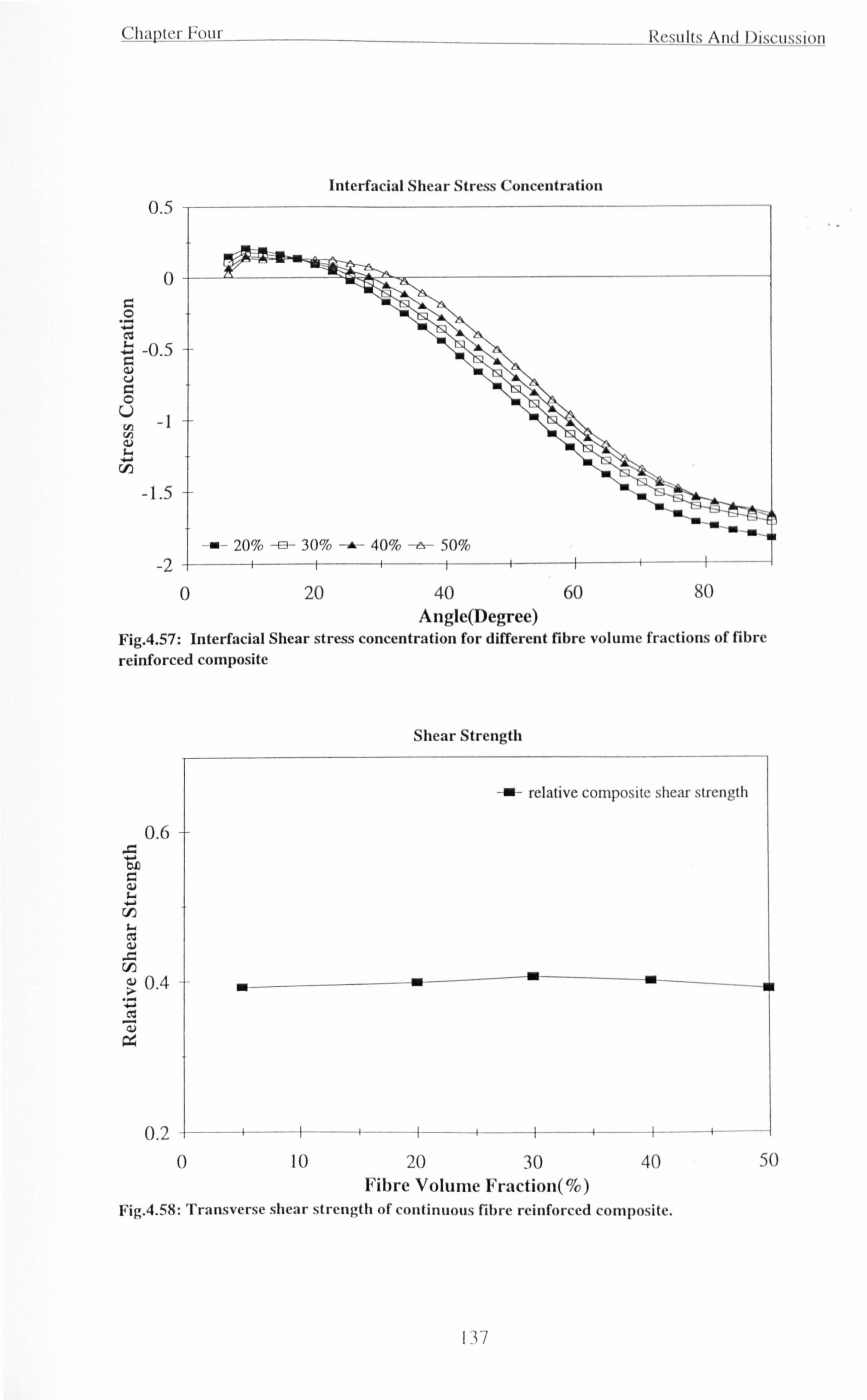
CIripterFuur
0.5 -r
Lxs....,. ý 0 ý ý -0.5 au U ý C L)
-1 C, ) C) L
ý cn
-1.5 A ?ý aý _a_ ýs _
n` ý m0
11 20%-a-30%-A-40%--50%
-2 t+-, -- f
0 20 40 60 80 Angle(Degree)
Fig. 4.57: Interfacial Shear stress concentration for different fibre volume fractions of fibre
reinforced composite
Shear Strength
relative composite shear strength
ý ýn c aý c. ý ý L.
cý aý
0.6
ý > 0.4 .ý ý ý ý 9
M--
Interfacial Shear Stress Concentration
--ý
f ._. {{ 0.2 A- -----t--- -- -- -- - -- A--- -4
0 10 20 30 40 50 Fibre Volume Fraction(%)
Fig. 4.58: Transverse shear strength of continuous fibre reinforced composite.
I. czttIts i1 n( 11 )i. ticuý, siun
r . <., ý t1,9C>� I
137
Chapter Four Results And Discussion
The distribution of the radial stress concentrations at the interface of the fibre and
matrix for different volume fractions is shown in figure 4.56. In this case the maximum
stress concentration occurs at about 45° of the pole for all the volume fractions. As the
fibre volume fraction increases, the stress concentration at the interface becomes
smaller. The variation of the interfacial shear stress concentration with volume
fraction, shown in figure 4.57, indicates an insignificant increase of the stress
concentration with increasing volume fraction of fibre.
The shear strength of composite obtained for different volume fractions is shown in
figure 4.58. These values are calculated using the maximum Von Mises concentrations
in the matrix. Although good quantitative predictions are not obtained for shear
strength by our model, still it can give a prediction for the variation of the strength
with the volume fraction qualitatively. As it can be seen in figure 4.58 the shear
strength of the composite hardly changes with the volume fraction.
There is a considerable resistance to shear fracture of the fibres. Hence this mode of
fracture is unlikely to occur and matrix failure can be blunted by fibres.
"w
138
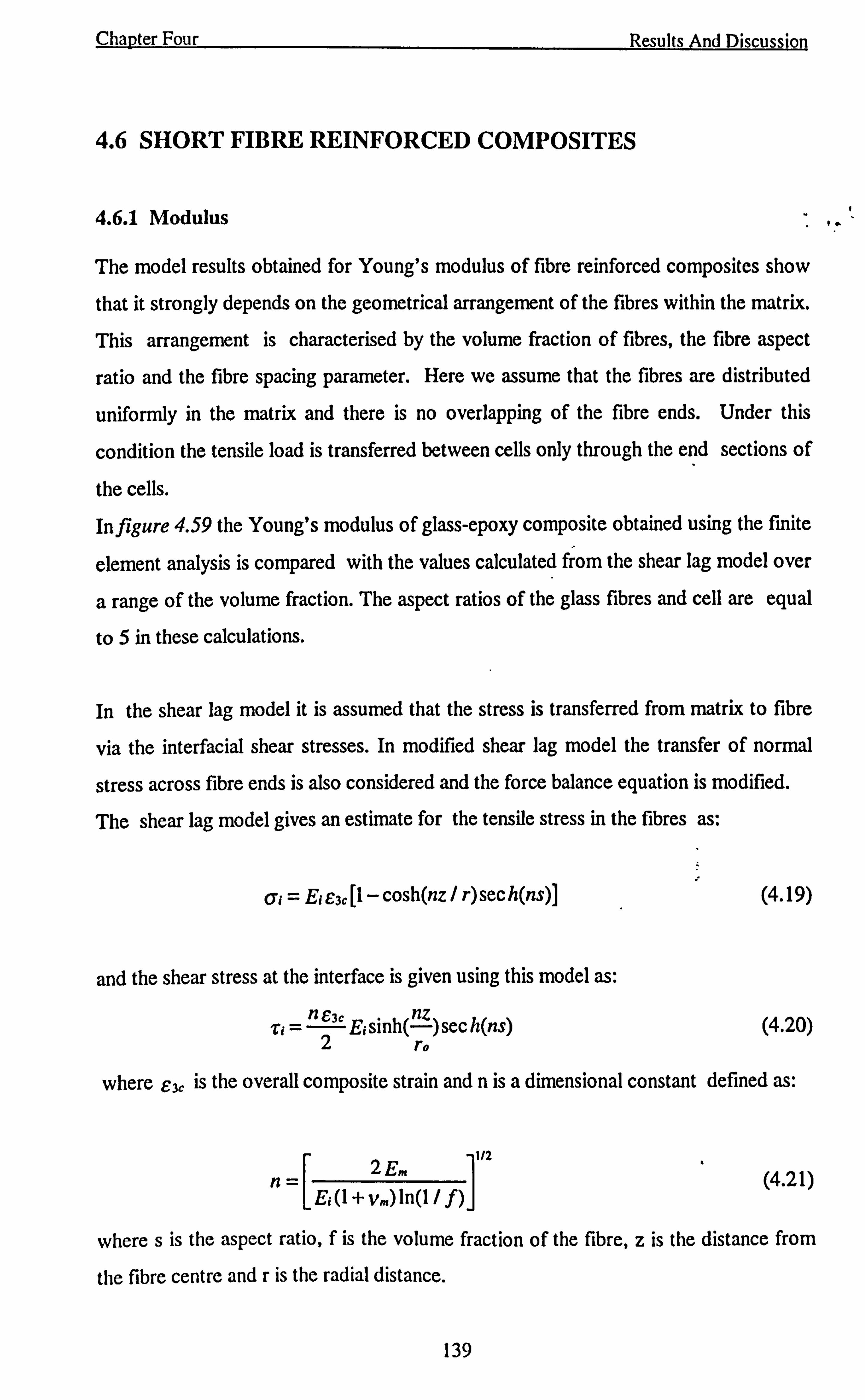
Chapter Four Results And Discussion
4.6 SHORT FIBRE REINFORCED COMPOSITES
4.6.1 Modulus
The model results obtained for Young's modulus of fibre reinforced composites show
that it strongly depends on the geometrical arrangement of the fibres within the matrix.
This arrangement is characterised by the volume fraction of fibres, the fibre aspect
ratio and the fibre spacing parameter. Here we assume that the fibres are distributed
uniformly in the matrix and there is no overlapping of the fibre ends. Under this
condition the tensile load is transferred between cells only through the end sections of
the cells.
In figure 4.59 the Young's modulus of glass-epoxy composite obtained using the finite
element analysis is compared with the values calculated from the shear lag model over
a range of the volume fraction. The aspect ratios of the glass fibres and cell are equal
to 5 in these calculations.
In the shear lag model it is assumed that the stress is transferred from matrix to fibre
via the interfacial shear stresses. In modified shear lag model the transfer of normal
stress across fibre ends is also considered and the force balance equation is modified.
The shear lag model gives an estimate for the tensile stress in the fibres as:
6; = Ei E3c [1- cosh(nz / r) sec h(ns)] (4.19)
and the shear stress at the interface is given using this model as:
z, =n E3c E; sinh( nz ) sec h(ns) 2 ro
(4.20)
where E3c is the overall composite strain and n is a dimensional constant defined as:
2 Em 1/2
E; (1 + vm) In(1 / f) (4.21)
where s is the aspect ratio, f is the volume fraction of the fibre, z is the distance from
the fibre centre and r is the radial distance.
1"
139
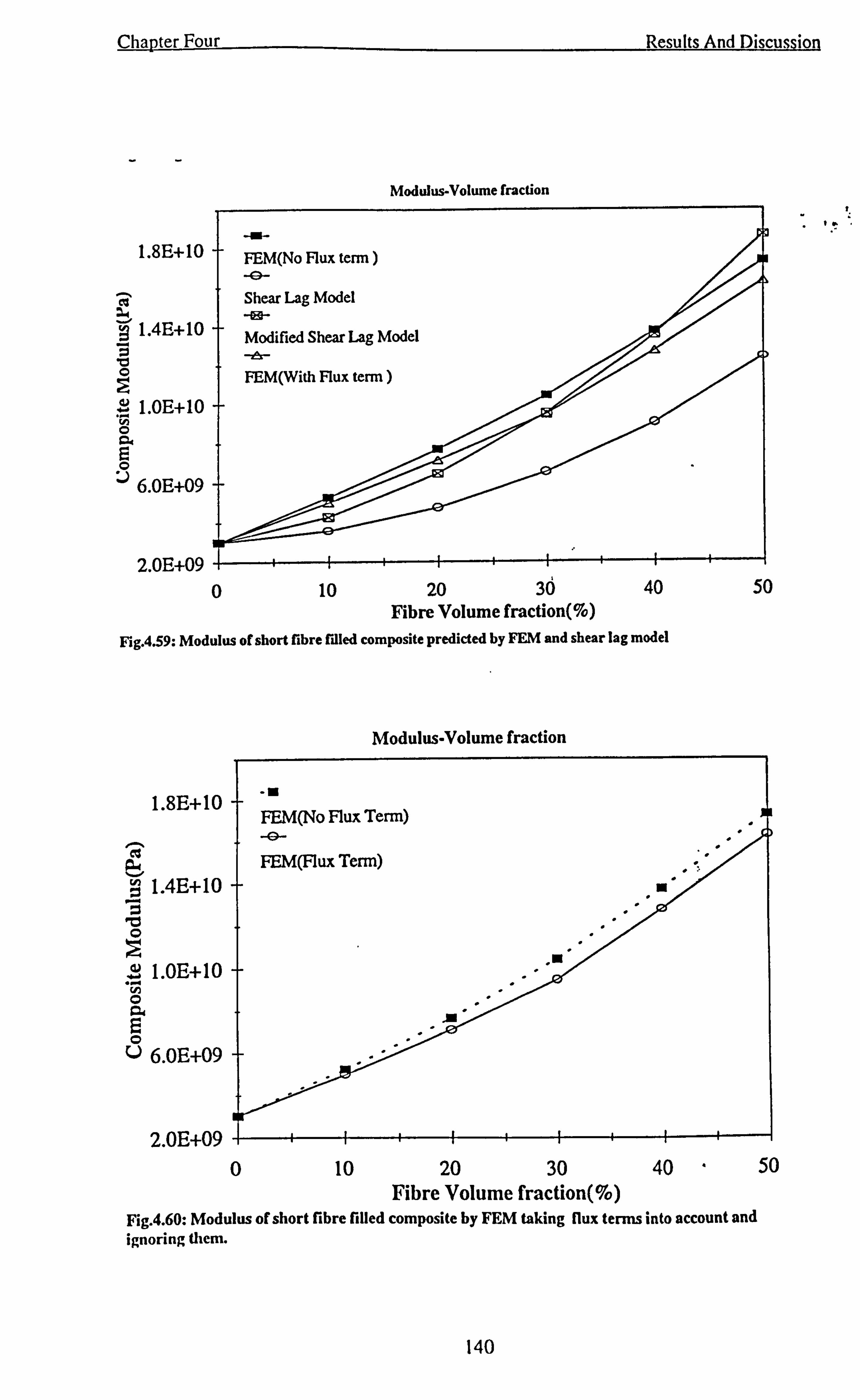
Chapter Four
Modulus-Volume fraction
Results And Discussion
1w
1.4E+10 0 ti 0
ý 1.0E+10 ý 0 a ý
6.0E+09
0 10 50 20 30 40 Fibre Volume fraction(%)
Fig. 4.59: Modulus of short fibre filled composite predicted by FEM and shear lag model
Modulus-Volume fraction
1.8E+10 FEM(No Flux Term) -9-
FEM(Flux Term) 1.4E+10
ý "O 0
1.0E+10 .ý y
0 a E
6.0E+09
2.0E+09 -+ 0 10 20 30 40 50
Fibre Volume fraction(%) Fig. 4.60: Modulus of short fibre filled composite by FEM taking flux terms into account and ignoring them.
140
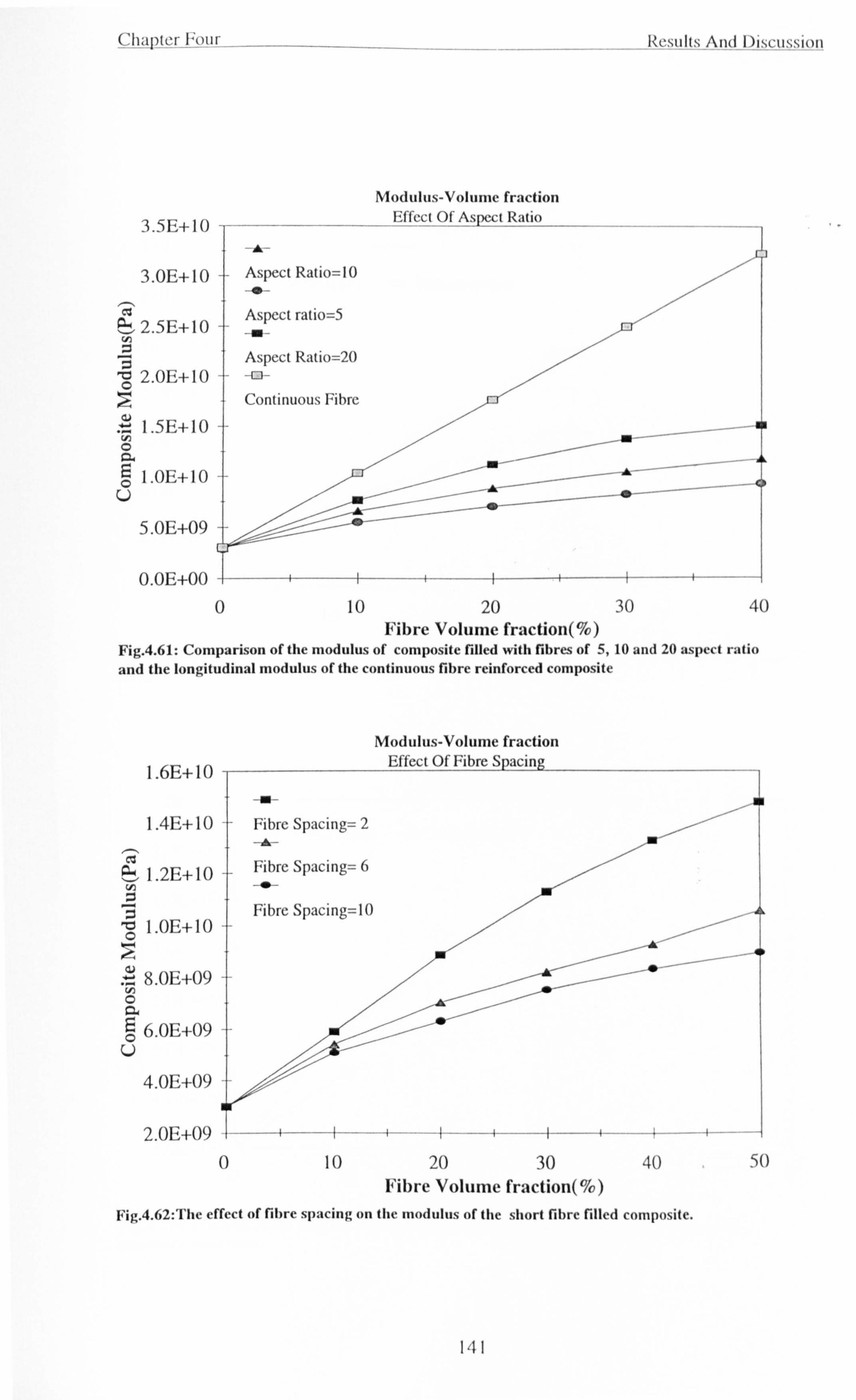
Chapter Four
3.5E+10
O. 0E+00 J
0 40
Fig. 4.61: Comparison of the modulus of composite filled with fibres of 5,10 and 20 aspect ratio and the longitudinal modulus of the continuous fibre reinforced composite
1.6E+10 ,
1.4E+ 10
, -. cý
Results And I )isrussiun
Modulus-Volume fraction Effccl OF Aspect Ratio--
ý
Modulus-Volume fraction Effect Of Fibre Spacing
-0- Fibre Spacing= 2
-A Fibre Spacing= 6
{
10 20 30 Fibre Volume fraction(%)
_. 411
2. OC+09 I
0 -+ ---j ---- -- -4- -1 -- i ---I
10 20 30 40 50 Fibre Volume fraction(%)
Fig. 4.62: The effect of fibre spacing on the modulus of the short fibre filled composite.
141
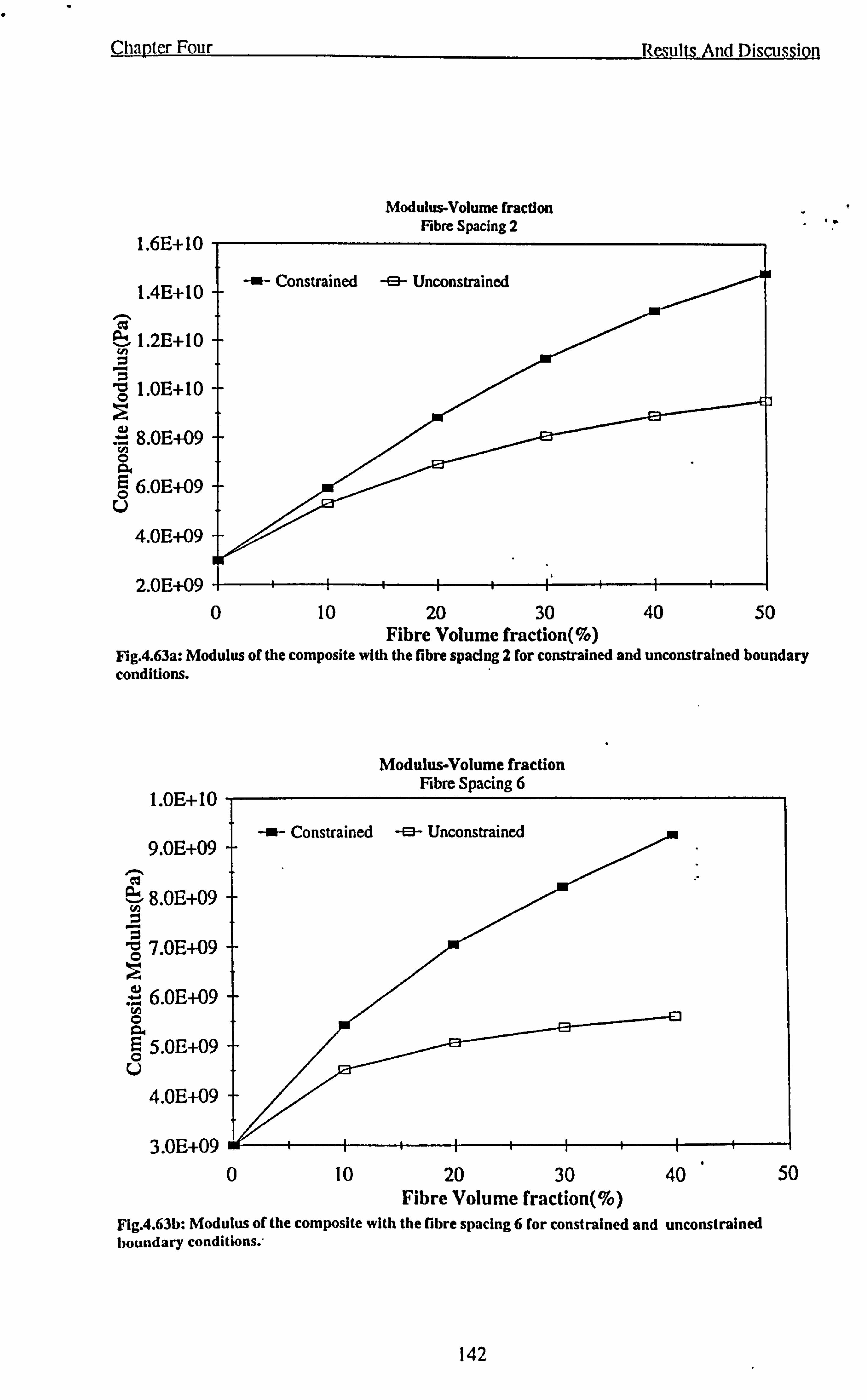
Chapter Four
1.6E+10 ,
2.0E+09
0 10
Modulus-Volume fraction Fibre Spacing 2
Results And Discussion
20 30 40 50 Fibre Volume fraction(%)
Fig. 4.63a: Modulus of the composite with the fibre spacing 2 for constrained and unconstrained boundary conditions.
1.0E+10
9.0E+09 . -. 2
8.0E+09
c 7.0E+09
6.0E+09 ý 0 a 9 5.0E+09 Q
U
0
Modulus-Volume fraction Fibre Spacing 6
-ý- Constrained -e- Unconstrained
10 20 30 Fibre Volume fraction(%)
40
Fig. 4.63b: Modulus of the composite with the fibre spacing 6 for constrained and unconstrained boundary conditions. -
50
142
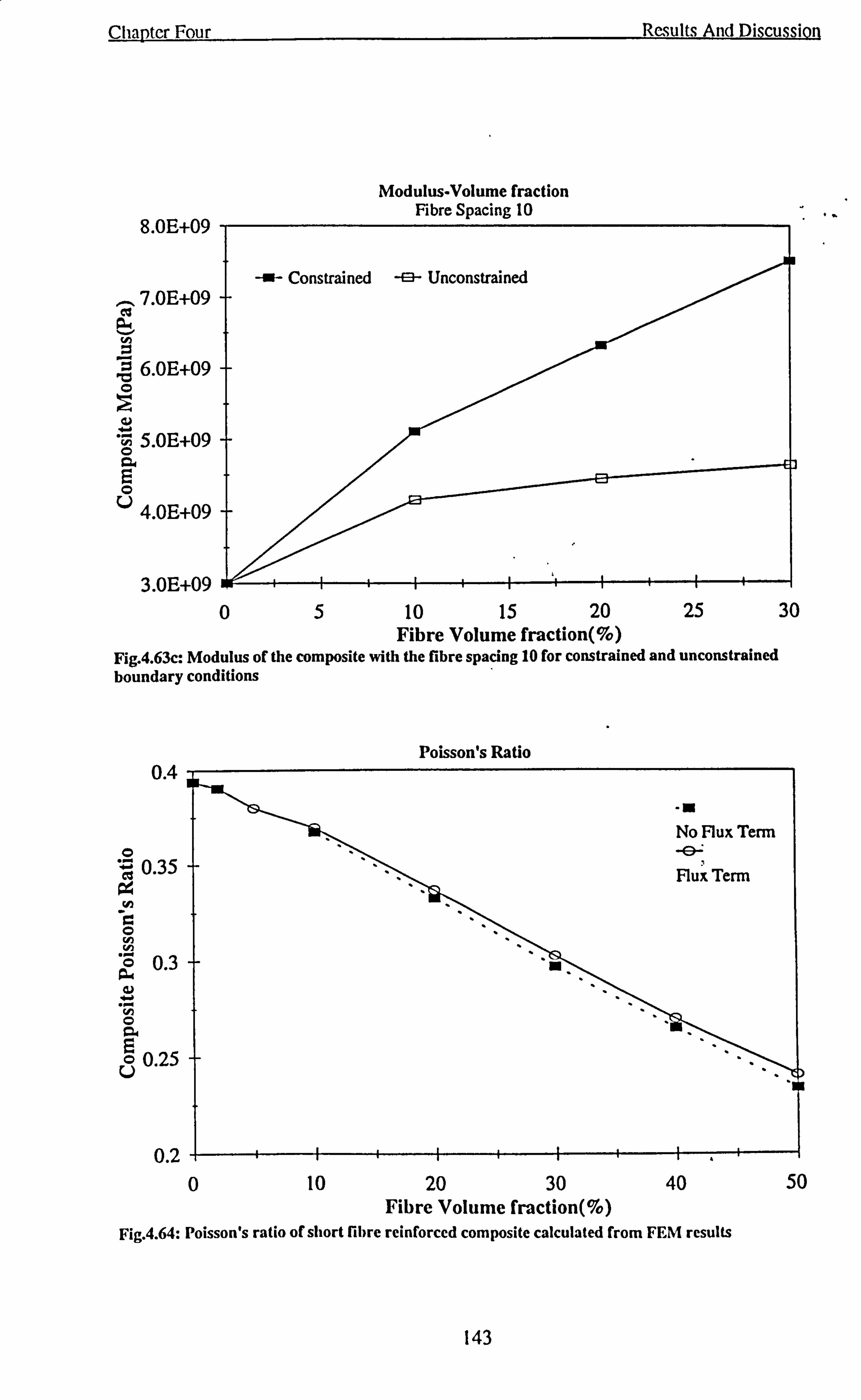
Chapter Four
8.0E+09
,.. 7.0E+09
6.0E+09 0
ý
aý ý 5. OE+09 O
O
U 4.0E+09 ý
3.0E+09
0
Modulus-Volume fraction Fibre Spacing 10
Results And Discussion
-ý- Constrained -0- Unconstrained
5 10 15 20 25 30 Fibre Volume fraction(%)
Fig. 4.63c: Modulus of the composite with the fibre spacing 10 for constrained and unconstrained boundary conditions
Poisson's Ratio
0.2 -+ 0 10 20 30
Fibre Volume fraction(%) 40 50
Fig. 4.64: Poisson's ratio of short fibre reinforced composite calculated from FEM results
143
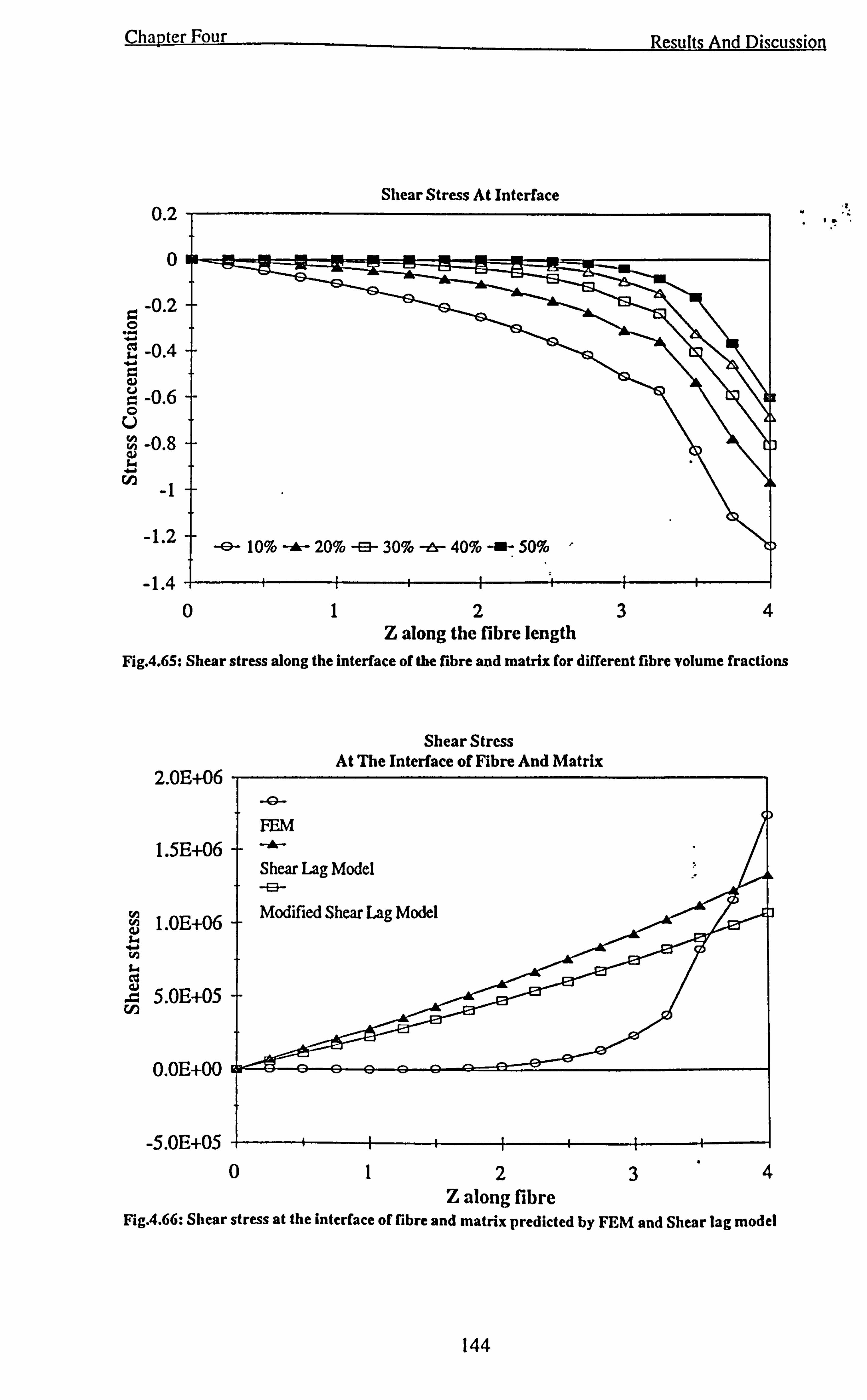
Chapter Four
0.2
0
ý -0.2 0 .., .ý ý -0.4 ý ý aý ý -0.6 0 U ý -0.8 ý ý'
-1
-1.2
-1.4
Shear Stress At Interface
012 Z along the fibre length
3
Results And Discussion
4
Fig. 4.65: Shear stress along the interface of the fibre and matrix for different fibre volume fractions
Shear Stress At The Interface of Fibre And Matrix
2.0E+06
1.5E+06
1.0E+06
5.0E+05
0.0E+00
-5.0E+05
-0-
FEM -, Ar- Shear Lag Model -a- Modified Shear Lag Model
012 Z along fibre
3 4
Fig. 4.66: Shear stress at the interface of fibre and matrix predicted by FEM and Shear lag model
144
Chapter Four Results And Discussion
The shear lag model gives much lower values for modulus. The values of moduli found
by modified shear lag model are closer to the finite element results.
In implementing the finite element analysis first the boundary tractions at the interface
of the fibre and matrix are ignored. Then the calculations are repeated and the
boundary flux terms are considered in the field equations. The moduli values found in
the latter analysis are lower than the results obtained from the no boundary traction
case. This comparison is shown in figure 4.60.
The effect of different fibre aspect ratios at constant fibre spacing on the composite
modulus is investigated. In figure 4.61 the variations of the modulus of glass epoxy
composite for the aspect ratios of 5,10 and 20 are shown. The fibre spacing is 6 in all
of these cases. A relative increase of the modulus can be. observed with the increase of
the aspect ratio. The upper limit is the longitudinal modulus of the continuous fibres
that can be achieved by using fibres with high aspect ratio.
The modulus of the composites filled with rod shape particles also depends on the fibre
spacing. The variations of the modulus for three different fibre spacing of 2,6 and 10
at constant aspect ratio of 5 is shown in figure 4.62. There is a decrease in modulus as
the fibre spacing increases.
The boundary condition on the side wall of the cell can be with constraint. In this case
the final stress distribution and effective properties of the composite should be
calculated by superimposing the results of the two steps are described in the chapter
3. The unconstrained boundary condition is also modelled. The results of the two sets
of the boundary conditions are compared in figures 4.63a-c. A remarkable difference
can be observed between the two cases. The imposition of unconstrained boundary
condition results in much lower values of the modulus.
The Poisson's ratio values are given in figure 4.64 for both cases of with and without
flux terms in the model equations.
145
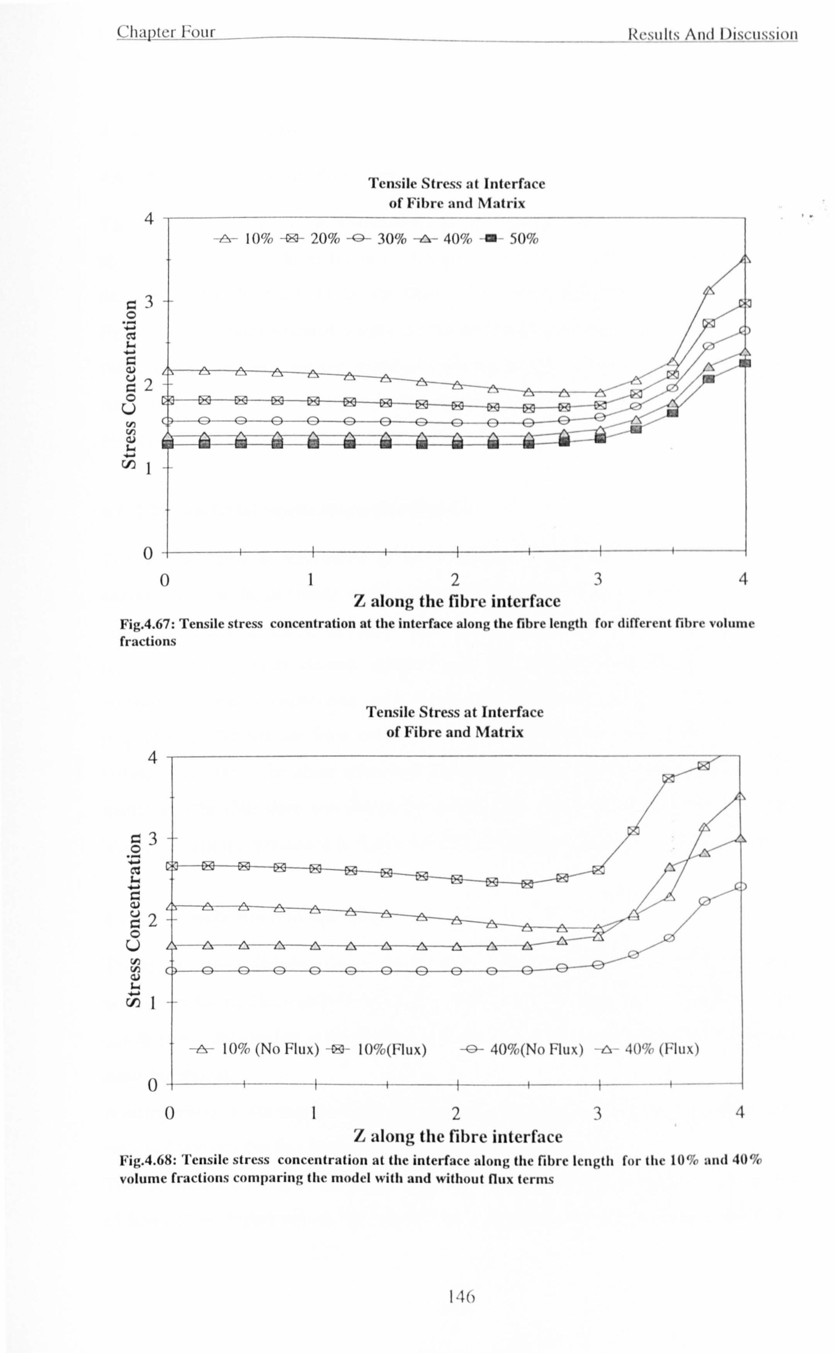
ChapterFour I; (-stills And I )isru,,. tii, ui
Tensile Stress at Interface
of Fibre and Matrix
0
-ý
2 Z along the fibre interface
3 4
Fig. 4.67: Tensile stress concentration at the interface along the fibre length for different fibre volume fractions
Tensile Stress at Interface
of Fibre and Matrix
vý1
0 234 Z along the fibre interface
Fig. 4.68: Tensile stress concentration at the interface along the fibre length for the 10% and 40%
volume fractions comparing the model with and without flux terms
10% (No Flux) -0- 10%(Flux)
QA
-0- 40%(No Flux) --a- 40% (Flux)
-- --- f- - ----+ --ý iý
ý,
I-10
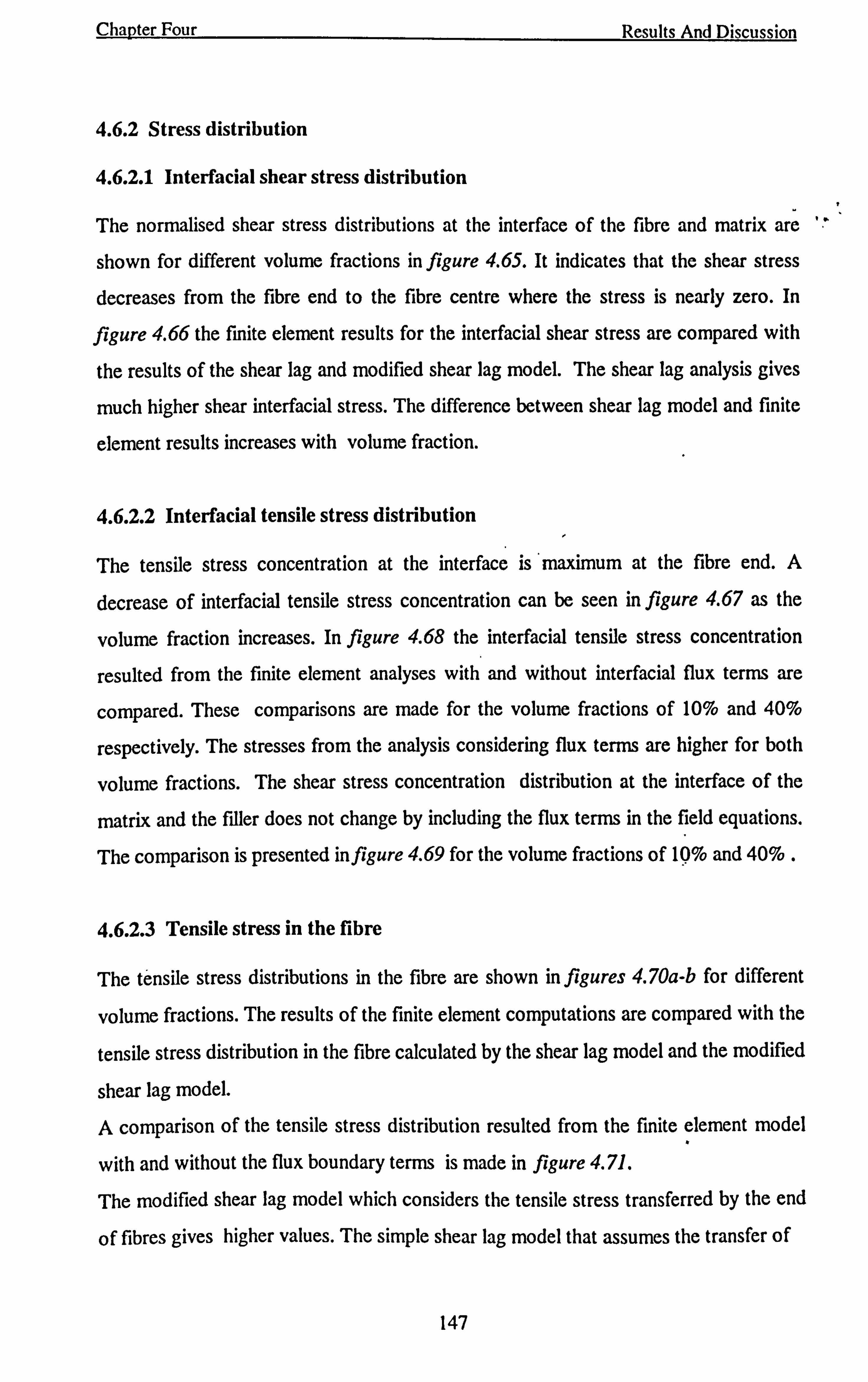
Chapter Four Results And Discussion
4.6.2 Stress distribution
4.6.2.1 Interfacial shear stress distribution
The normalised shear stress distributions at the interface of the fibre and matrix are
shown for different volume fractions in figure 4.65. It indicates that the shear stress
decreases from the fibre end to the fibre centre where the stress is nearly zero. In
figure 4.66 the finite element results for the interfacial shear stress are compared with
the results of the shear lag and modified shear lag model. The shear lag analysis gives
much higher shear interfacial stress. The difference between shear lag model and finite
element results increases with volume fraction.
4.6.2.2 Interfacial tensile stress distribution
The tensile stress concentration at the interface is maximum at the fibre end. A
decrease of interfacial tensile stress concentration can be seen in figure 4.67 as the
volume fraction increases. In figure 4.68 the interfacial tensile stress concentration
resulted from the finite element analyses with and without interfacial flux terms are
compared. These comparisons are made for the volume fractions of 10% and 40%
respectively. The stresses from the analysis considering flux terms are higher for both
volume fractions. The shear stress concentration distribution at the interface of the
matrix and the filler does not change by including the flux terms in the field equations.
The comparison is presented in figure 4.69 for the volume fractions of 10% and 40% .
4.6.2.3 Tensile stress in the fibre
The tensile stress distributions in the fibre are shown in figures 4.70a-b for different
volume fractions. The results of the finite element computations are compared with the
tensile stress distribution in the fibre calculated by the shear lag model and the modified
shear lag model.
A comparison of the tensile stress distribution resulted from the finite element model
with and without the flux boundary terms is made in figure 4.71.
The modified shear lag model which considers the tensile stress transferred by the end
of fibres gives higher values. The simple shear lag model that assumes the transfer of
ýw
147
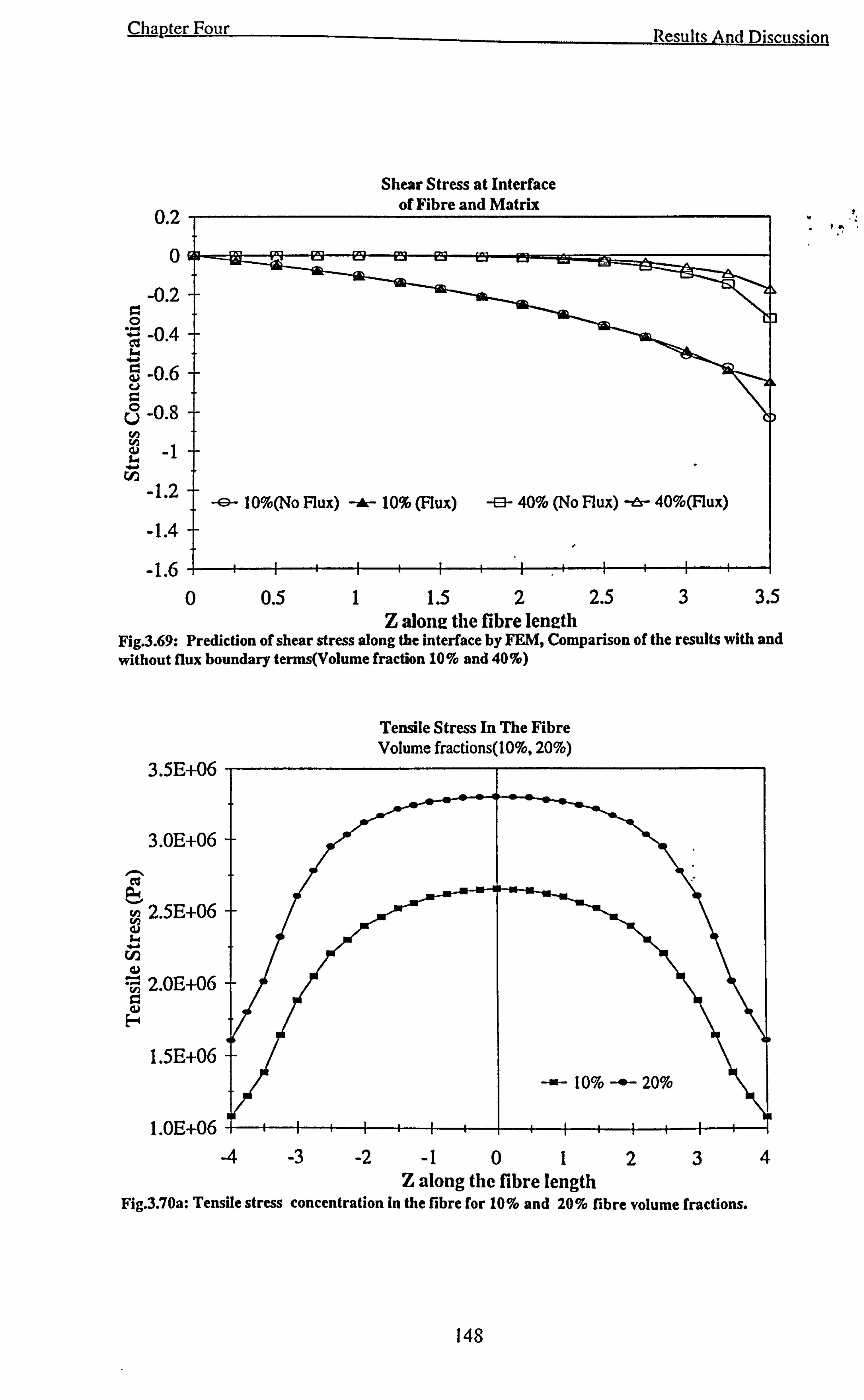
Chapter Four
0.2
0 -0.2
O
- -0.4 ý ý -0.6 u ý Ü -0.8 ý aý -1 ý. ý ý 1.2
-1.4
-1.6 0 0.5
Shear Stress at Interface
of Fibre and Matrix
1 1.5 2 2.5 3 3.5 Z along the fibre length
Fig. 3.69: Prediction of shear stress along the interface by FEM, Comparison of the results with and without flux boundary terms(Volume fraction 10% and 40%)
Tensile Stress In The Fibre Volume fractions(10%, 20%)
-4 -3 -2 -1 012 Z along the fibre length
Results And Discussion
3
Fig. 3.70a: Tensile stress concentration in the fibre for 10% and 20% fibre volume fractions.
4
148
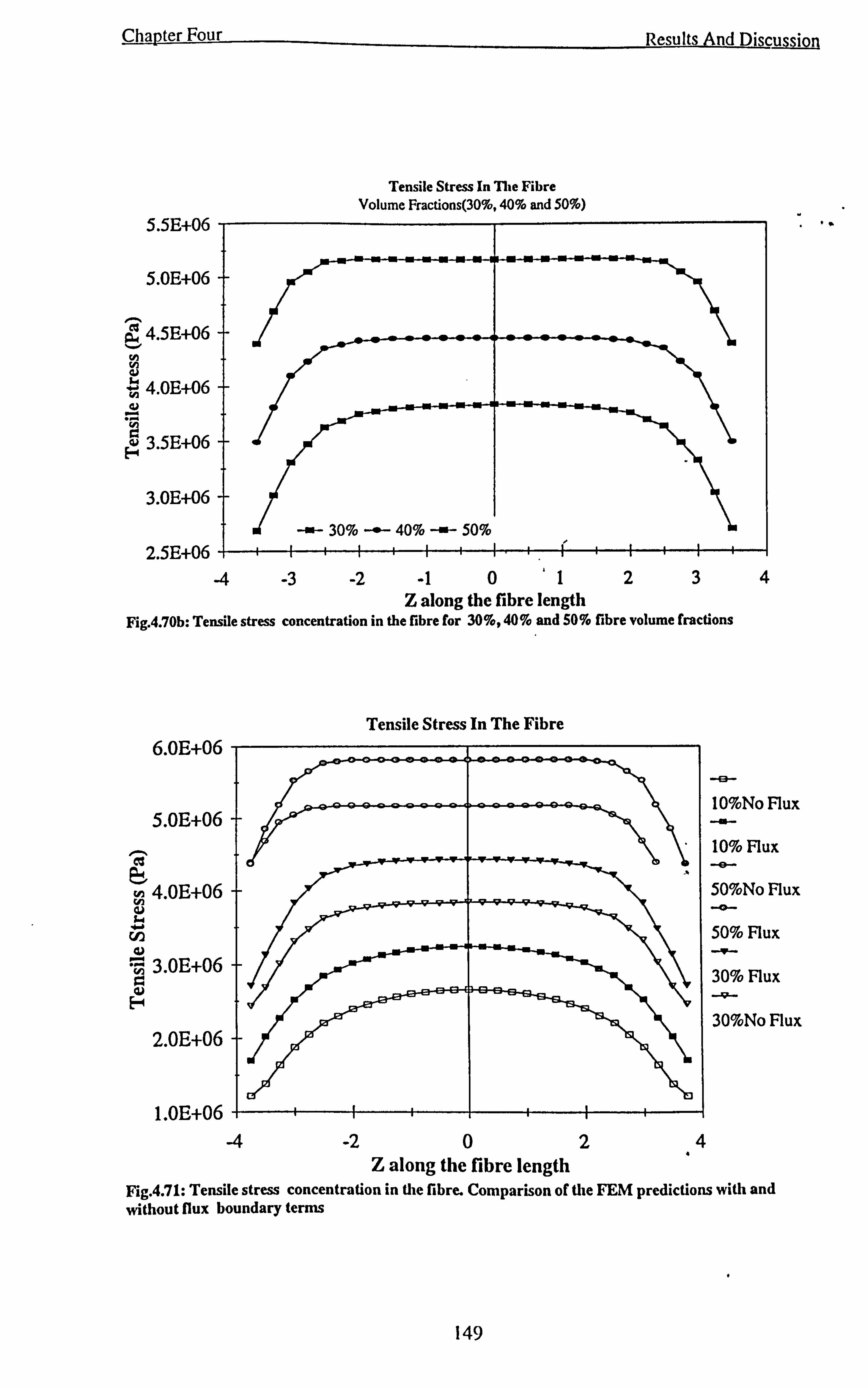
Chapter Four
Tensile Stress In The Fibre Volume Fractions(30%, 40% and 50%)
5.5E+06
5.0E+06
4.5E+06 ti h 4.0E+06 4) .ý ...
Eý 3.5E+06
3.0E+06
2.5E+06
-4 -3 -2 -1 012 Z along the fibre length
ýý -ý - 30% -+- 40% -ý- 50% I-r-I-r-I-j-I
Results And Discussion
3 4
Fig. 4.70b: Tensile stress concentration in the fibre for 30%, 40% and 50% fibre volume fractions
Tensile Stress In The Fibre
5.0E+06 -F
RS ý
4.0E+06 f W3
CL)
3.0E+06
E-+
-2 02 Z along the fibre length
10%No Flux
10% Flux -e-. 50%No Flux
50% Flux
30% Flux
30%No Flux
Fig. 4.71: Tensile stress concentration in the fibre. Comparison of the FEM predictions with and without flux boundary terms
149
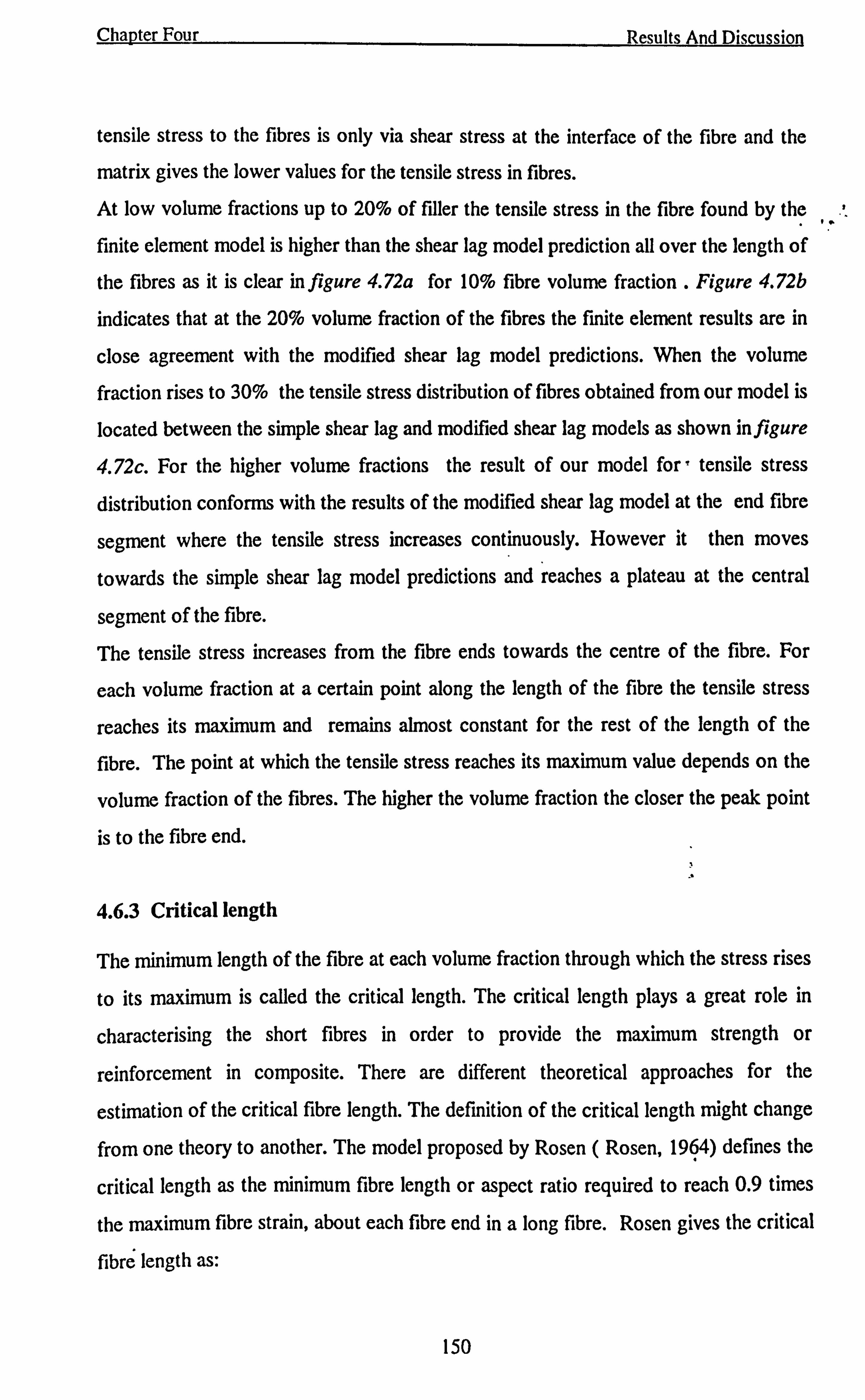
Chapter Four Results And Discussion
tensile stress to the fibres is only via shear stress at the interface of the fibre and the
matrix gives the lower values for the tensile stress in fibres.
At low volume fractions up to 20% of filler the tensile stress in the fibre found by the
finite element model is higher than the shear lag model prediction all over the length of
the fibres as it is clear in figure 4.72a for 10% fibre volume fraction . Figure 4.72b
indicates that at the 20% volume fraction of the fibres the finite element results are in
close agreement with the modified shear lag model predictions. When the volume
fraction rises to 30% the tensile stress distribution of fibres obtained from our model is
located between the simple shear lag and modified shear lag models as shown in figure
4.72c. For the higher volume fractions the result of our model for, tensile stress
distribution conforms with the results of the modified shear lag model at the end fibre
segment where the tensile stress increases continuously. However it then moves
towards the simple shear lag model predictions and reaches a plateau at the central
segment of the fibre.
The tensile stress increases from the fibre ends towards the centre of the fibre. For
each volume fraction at a certain point along the length of the fibre the tensile stress
reaches its maximum and remains almost constant for the rest of the length of the
fibre. The point at which the tensile stress reaches its maximum value depends on the
volume fraction of the fibres. The higher the volume fraction the closer the peak point
is to the fibre end.
4.6.3 Critical length
The minimum length of the fibre at each volume fraction through which the stress rises
to its maximum is called the critical length. The critical length plays a great role in
characterising the short fibres in order to provide the maximum strength or
reinforcement in composite. There are different theoretical approaches for the
estimation of the critical fibre length. The definition of the critical length might change
from one theory to another. The model proposed by Rosen ( Rosen, 1964) defines the
critical length as the minimum fibre length or aspect ratio required to reach 0.9 times
the maximum fibre strain, about each fibre end in a long fibre. Rosen gives the critical
fibre length as:
ý.
150
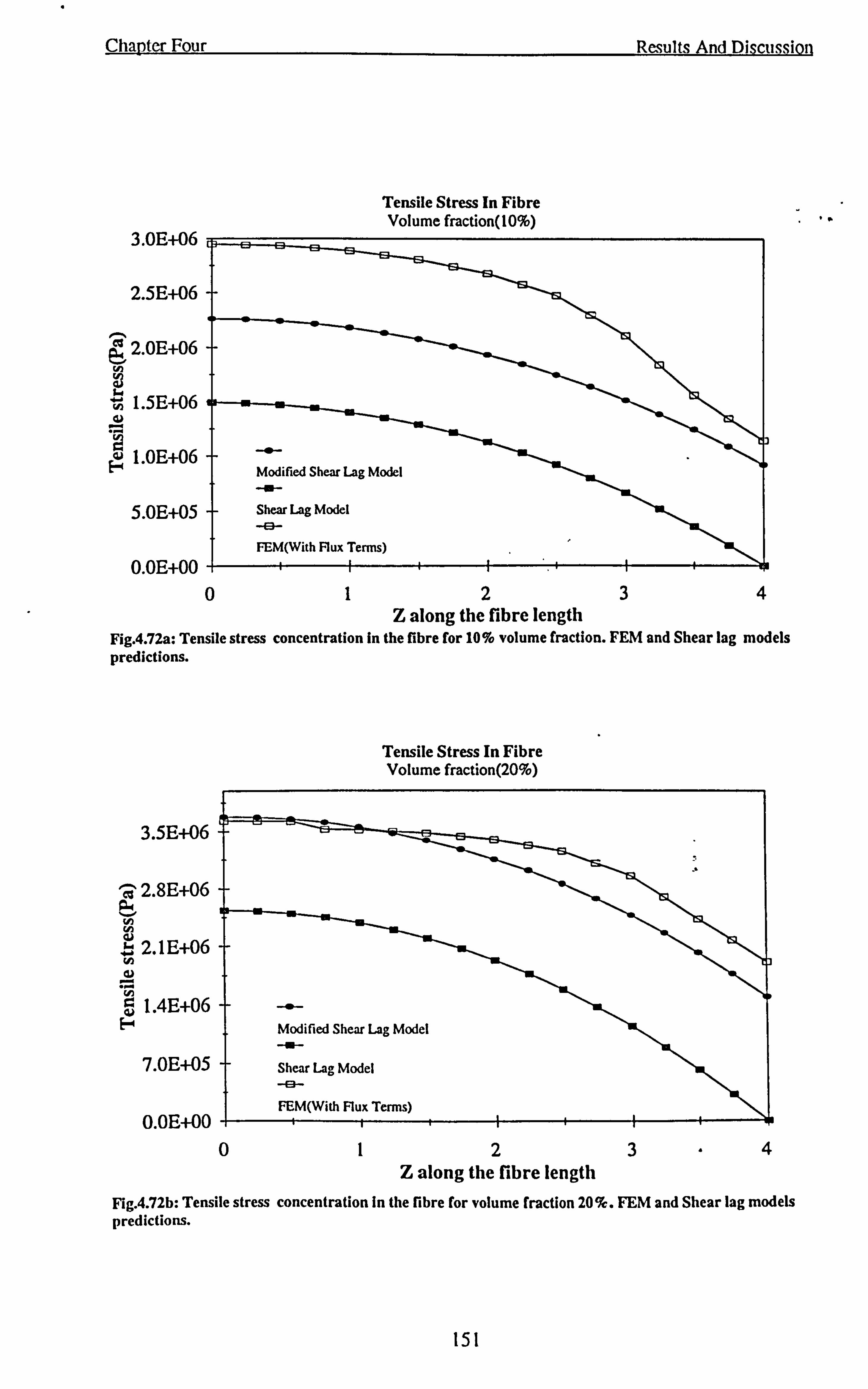
Chapter Four
3.0E+06
2.5E+06
2.0E+06 ý ý ý 1.5E+06
... 1.0E+06
5.0E+05
0.0E+00
0
Results And Discussion
1
Tensile Stress In Fibre Volume fraction(10%)
2 Z along the fibre length
3 4
Fig. 4.72a: Tensile stress concentration in the fibre for 10% volume fraction. FEM and Shear lag models predictions.
Tensile Stress In Fibre Volume fraction(20%)
ý 2.8E+06 a ý ý rA
eLl ý 2.1 E+06
ý. .., 1.4E+06
F4
7.0E+05
0.0E+00 0
--"- Modified Shear Lag Model -a-- Shear Lag Model
-E3- FEM(With Flux Terms)
1 2 3
}
4 Z along the fibre length
Fig. 4.72b: Tensile stress concentration in the fibre for volume fraction 20%. FEM and Shear lag models predictions.
.'
151
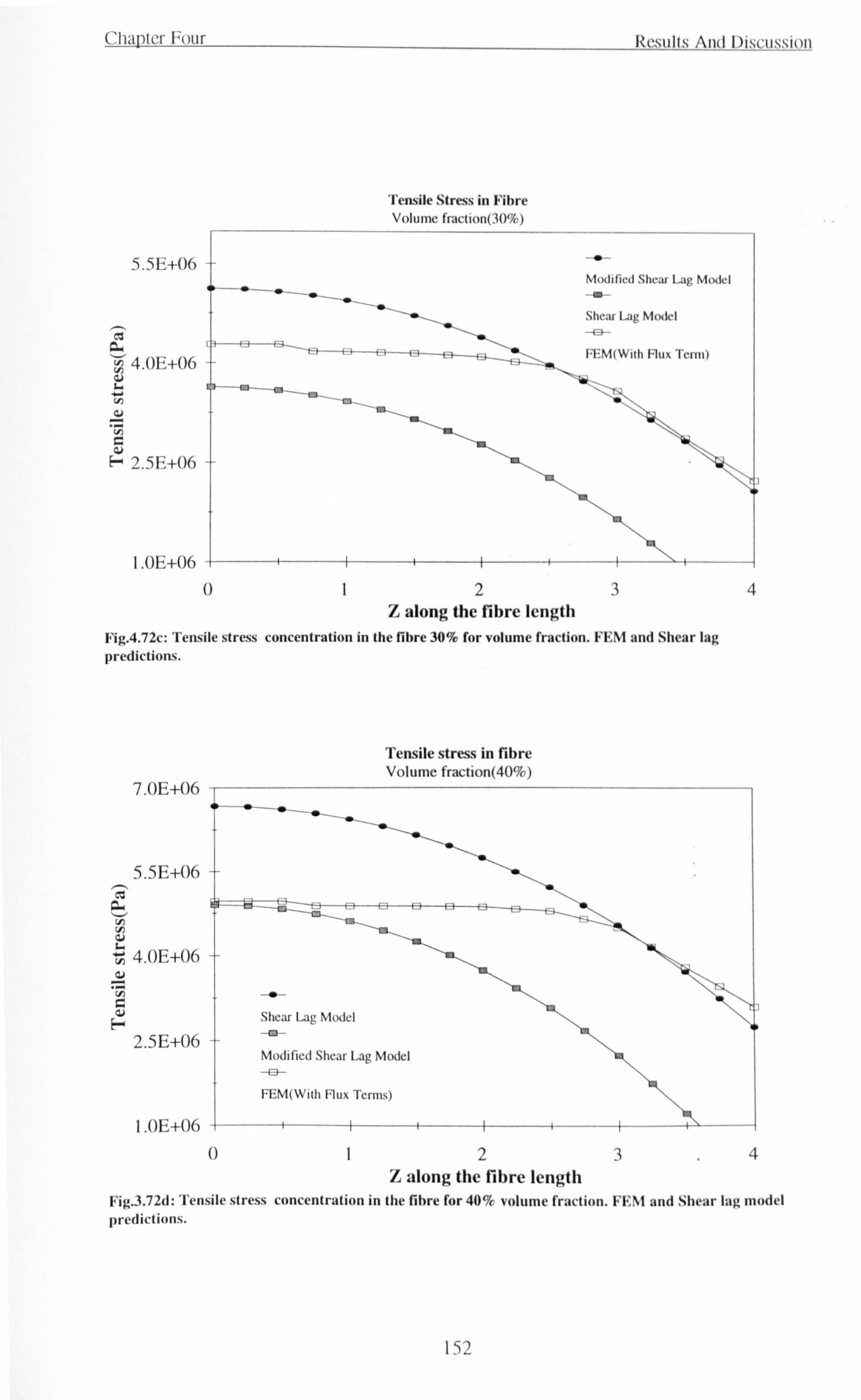
Chapter Four
5.5E+06
r-. ß 4.0E+06
ý.
ý
Fr 2.5E+06
1.0E+06
0
Fig. 4.72c: Tensile stress predictions.
7.0E+06
5.5E+06 , -.
4.0E+06
2.5E+06
1.0E+06
U
I. c. tiiil(s And I )isrus. tiioun
I
Tensile Stress in Fibre Volume fraction(30%)
2 Z along the fibre length
Modified Shear Lag Model m
Shear Lag Model
. -+3_ FEM(With hlux Term)
3
concentration in the fibre 30% for volume fraction. FEM and Shear lag
Tensile stress in fibre Volume fraction(40%)
Shear Lag Model
Modified Shear Lag Model
FEM(With Flux Terms)
+--
i 2 Z along the fibre length
4
4
Fig. 3.72d: Tensile stress concentration in the fibre for 40% volume fraction. FENI and Shear lag model predictions.
152
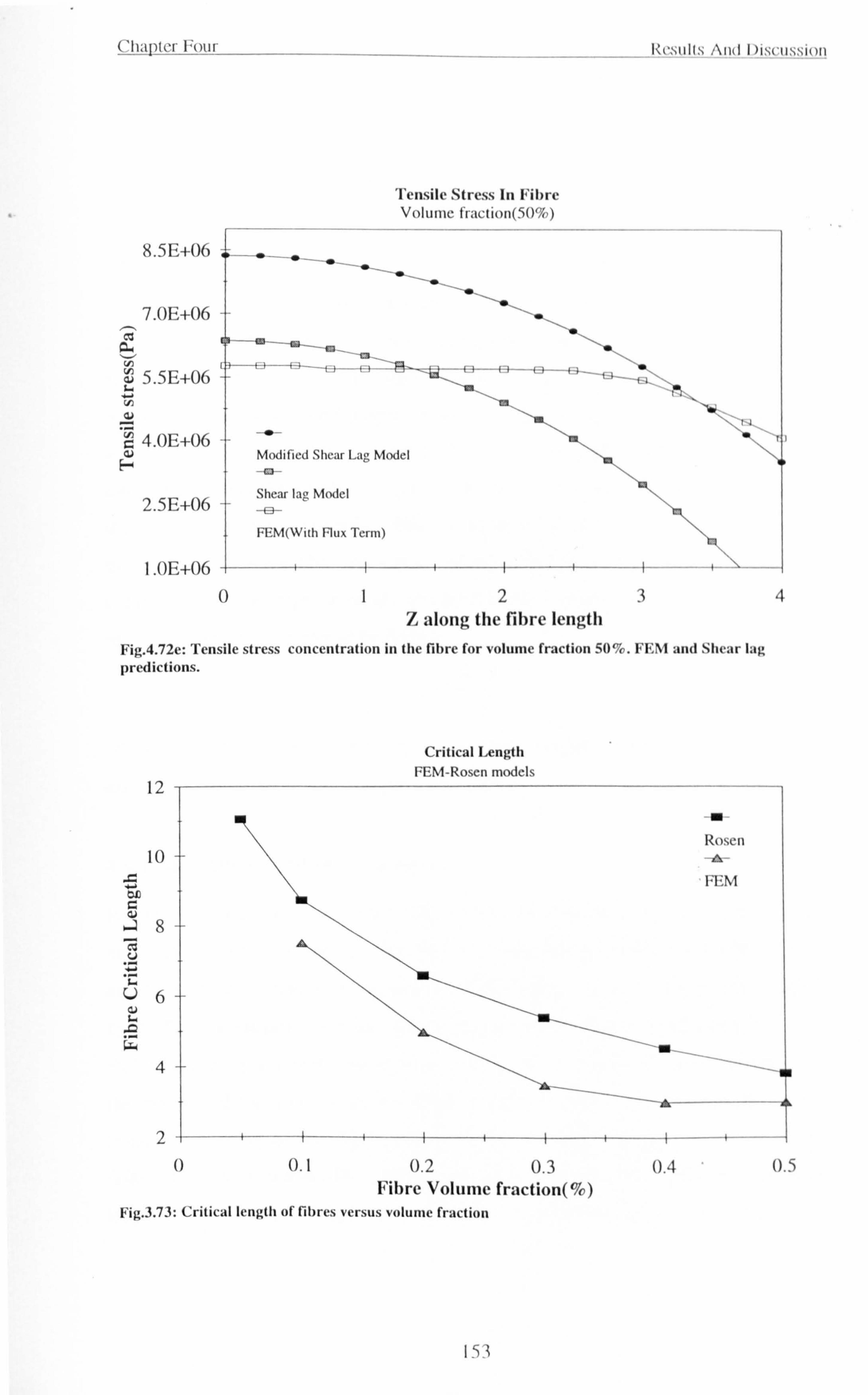
Chapter Four
Tensile Stress In Fibre Volume fraction(50%)
8.5E+06
ý 7.0E+06
-" ý
`ý\ýý
hrsuils And I >isrussiun
ý
I H
2.5E+06
Modified Shear Lag Model
Shear lag Model
1.0E+06 1+ i
012 Z along the fibre length
3 4
Fig. 4.72e: Tensile stress concentration in the fibre for volume fraction 50%. FRA1 and Shear lag
predictions.
Critical Length FENI-Rosen models
12
-0
10 Rosen
I&- FEM
8 -I
6+
4
24i i- iIi, ii ---i
0 0.1 0.2 0.3 0.4 0.5 Fibre Volume fraction(%)
Fig. 3.73: Critical length of fibres versus volume fraction
153
Chapter Four Results And Discussion
Ef(1+vm) V2 Vf2 1/2 lý =dE Vv2 mf
(4.22)
where d is the fibre diameter, Ef and Vf are fibre Young's modulus and volume
fraction, v�, and E. are matrix Poisson's ratio and Young's modulus.
Equation 4.22 shows that the critical fibre length depends on the fibre diameter, the
square root of the ratio of the tensile moduli and on a term representing the fibre
volume fraction. The critical lengths of fibres obtained by the finite element model and
Rosen model are compared in figure 4.73 for a range of filler volume fractions. Our
model shows that the tensile stress in the fibre rises to its peak in a shorter length of
the fibre. Termonia (Termonia, 1990) concluded that the critical fibre length is a
unique function of the fibre and matrix modulus' ratio. But our results show that the
critical length also depends on the volume fraction. Another model which descirbes
the critical length is developed by Kelly as:
11 = a. r d 2zw
where d is the diameter of fibre, T. is the shear strength of the interface or of the
matrix and a, is the tensile strength of the fibre.
4.6.4 Strength of short fibre composites
Prediction of the strength of short fibre reinforced thermoplastics is a complex but
industrially crucial problem. In the case of a composite containing short fibres, the
existence of a non uniform stress along the fibre implies that the average stress carried
by the fibres at the point of failure will be less than fibre ultimate tensile strength.
Failure occurs by a different mechanism in the short fibre composite which depends on
the mechanical properties of the constituents and the tensile and shear strength of the
interfacial bonding of the fibres and the matrix. Another deterministic factor in the
failure mechanism in short fibre reinforced composites is the fibre aspect ratio or fibre
length. There is the possibility of failure in the fibre, in the matrix phase or at the
Em ýý Vi`
154
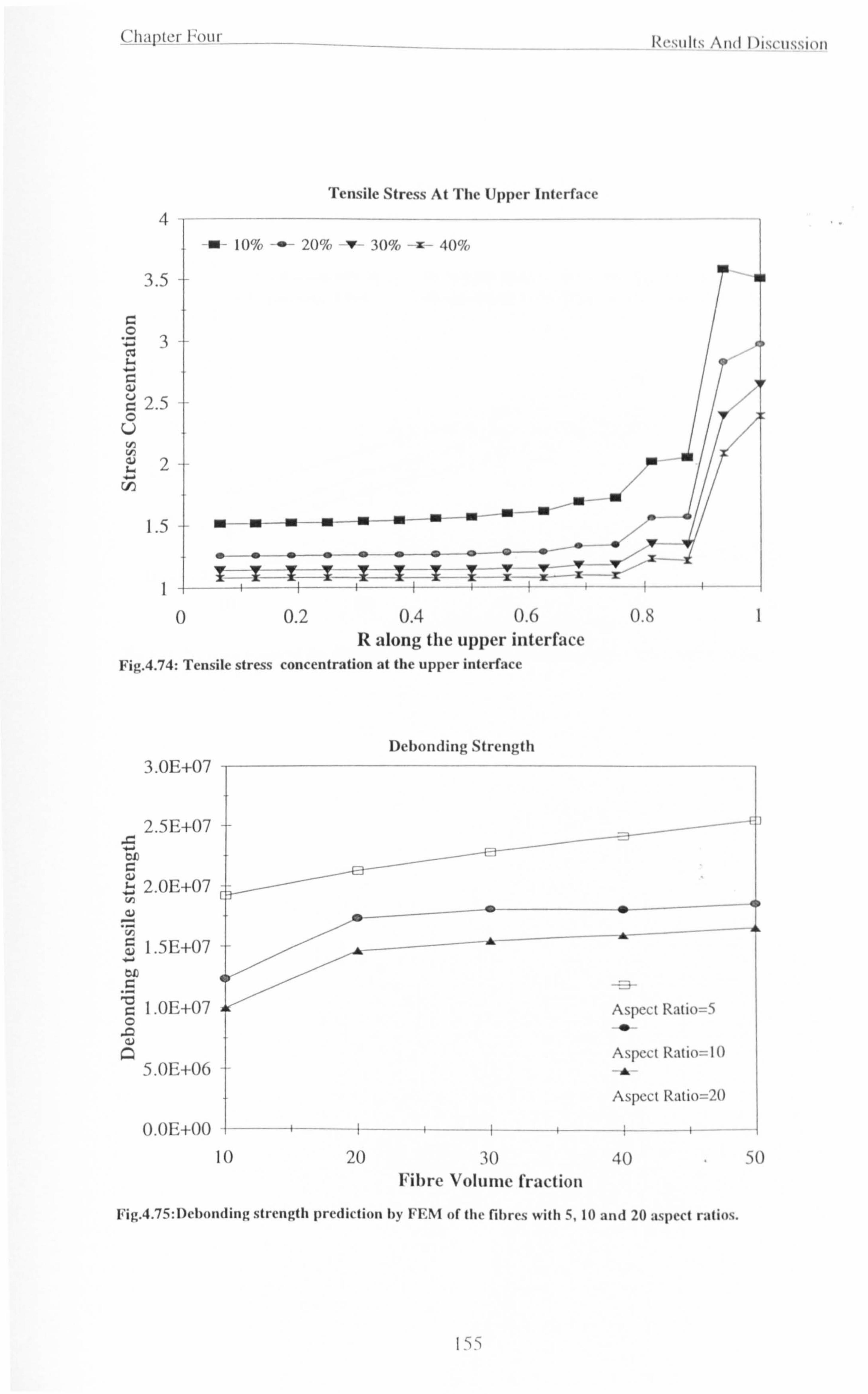
('haI)lrr Foul
3.5 -
ý 0 ý cý ý. 4.
ý 2.5 0 U ý ý 2 ý
1.5 -
Tensile Stress At The Upper Interface
m- 10% --- 2017, v- 30% -z- 40%
. -. a0 °---+ . -O
__________________________ ý --ý
ý T--4 ý-{
I: r. iill. ; \n l I1i` u. ti, i ui
w
m" -- . +ý, _v i
-i-=- -z/ 1--..
0 0.2 0.4 0.6 0.8 R along the upper interface
Fig. 4.74: Tensile stress concentration at the upper interface
3.0E+07
2.5E+07 4ý
an
2.0E+07
. C7 55 1.5E+07 ý an c
1.0E+07 0
_5. OE+0G
Aspect Ratio-5 "
Aspect Katiw I(1 A
Aspect Ratio=20
O. 0E+00 I-
IO --4--- -t -- -- --f- -- -- ý
20
Debonding Strength
a
I
30 40 50 Fibre Volume fraction
Fig. 4.75: Debonding strength prediction by FEM of the fibres with 5,10 and 20 aspect ratios.
i, -ý
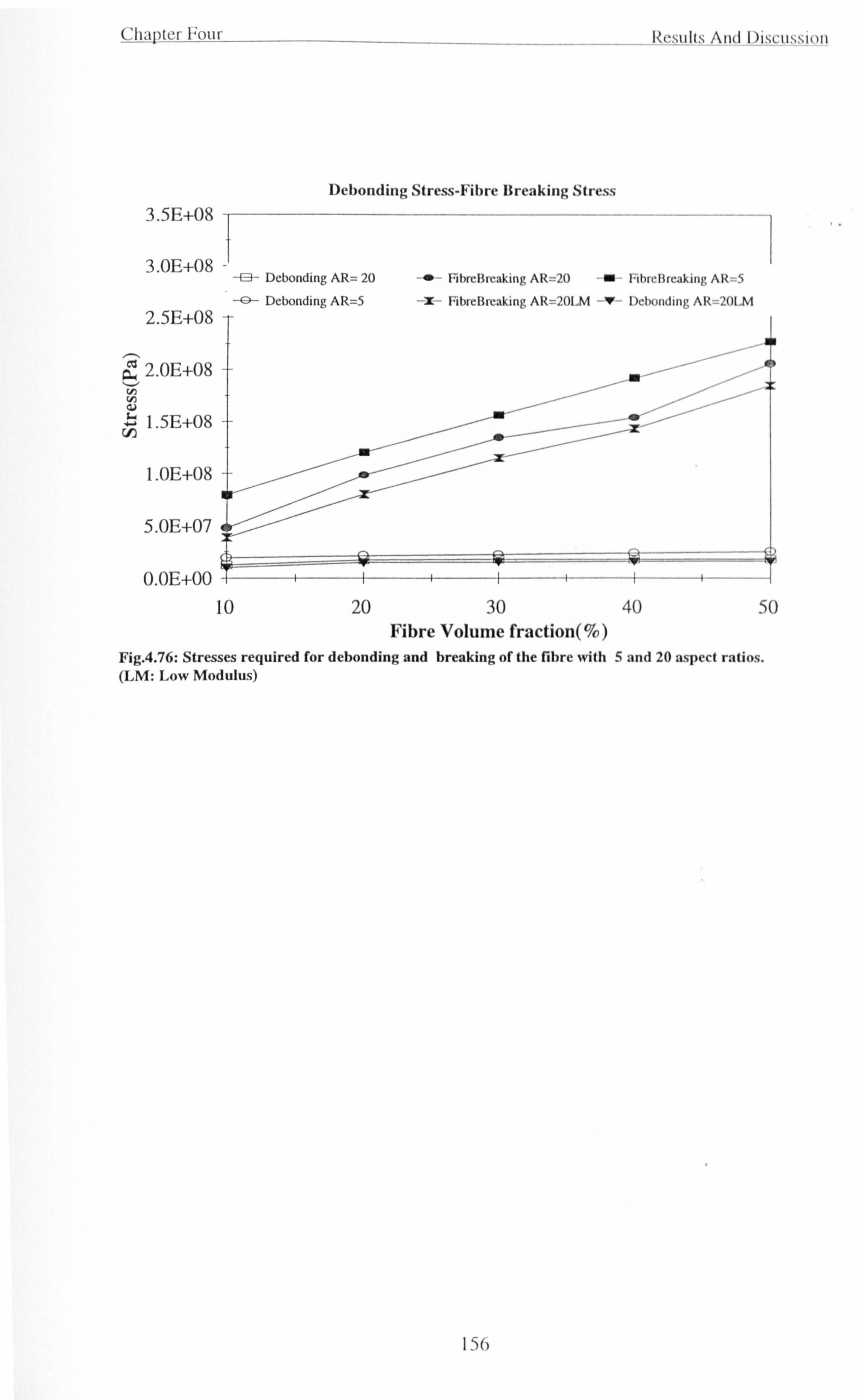
Chapter Four
3.5E+08
3.0E+08 -
Debonding Stress-Fibre Breaking Stress
Itrsulls And Uisrii,. i
-E3- Debonding AR= 20
-0 - Debonding AR=5 2.5E+08 -r
2.0E+08 .ý m
i ý
dý up O. 0E+00 Ti -i
10
-- - Fibreßreaking AR=20 M lýibrcßreaking AR=5
Z- Fibreßreaking AR=201. M V- Dctxmding AR-201, M
i-i
Ä
74
20 30 40 50 Fibre Volume fraction(%)
Fig. 4.76: Stresses required for debonding and breaking of the fibre with 5 and 20 aspect ratios. (LM: Low Modulus)
156
(I
Chapter Four Results, And Discussion
fibre/matrix interface. A combination of these mechanisms can lead to the catastrophic
failure in the composite.
The significant stress on the lateral interface of the fibre/matrix along the fibre length is
the shear stress. Even when the shear stress on this face exceeds the shear strength of
the bonding, the compressive forces normal to this interface retain the fibre and
matrix closed. The compressive forces are the result of the lateral contraction of the
matrix.
Figure 4.74 shows the normal stress distribution at the upper interface of the fibre
and the matrix . The normal stresses at this face are tensile and as can be seen in this
figure the concentration of these stresses increases from the axis towards the edge of
the fibre. The concentration of the tensile stress reduces as the volume fraction
increases.
The debonding of the interface occurs when the tensile stress reaches the tensile
strength of the interfacial bonding. The debonding stresses obtained by the finite
element model are presented in figure 4.75. The debonding stresses for the aspect
ratios of 5 and 20 are given for the range of the volume fraction. The debonding
stress rises as the volume fraction increases. At the aspect ratio of 5 the increase is
more significant than the aspect ratio of 20.
The tensile stress required to be applied to the composite to bring the fibres to their
failure tensile stress is given in figure 4.76. The applied stress to break the fibres is
higher for aspect ratio of 5 compared to the values of the aspect ratio of 20. An
increase in the stress to breaking point can be observed at higher volume fractions. The
stresses at the breaking point are much higher than the debonding stresses for the fibre
glass and epoxy matrix. These differences are more remarkable at lower fibre aspect
ratios.
Therefore it can be predicted that at low aspect ratios the debonding of the fibres acts
as the initiation mechanism for the failure and it is followed by the failure of the matrix
near the fibre ends. Since the aspect ratio of short fibre is low, the concentration of the
fibre ends is high and then the local cracks merge transversely from the direction of
the applied load.
157
Chapter Four Results And Discussion
The catastrophic failure of the short fibre filled composite can occur without any
breaking of the fibres. At higher aspect ratio, since the breaking stress of the fibres is
lower, the failure occurs in two steps. In the first step the interface debonding and Iw
tensile failure of the matrix at the fibre ends is observed. However, in contrast to the
low fibre aspect ratio case, growing matrix cracks at fibre ends are quickly blunted by
neighbouring fibres and hence no catastrophic failure occurs. Because of the cracks
and interfacial debonding the modulus of composite drops significantly.
Our model shows that the breaking stress of the fibres reduces at low modulus.
Therefore in the second step which corresponds to a decreased modulus the tensile
stress in the fibres can easily exceed the failure stress of the fibres leading to the
breakage of the fibres.
4
158

Chapter Five
CONCLUSION
5.1 CONCLUSIONS OF THE PRESENT WORK
The developed finite element model has proved to be a flexible and cost effective tool
for the prediction of properties of polymer composites. The stiffness, stress
concentration field, failure mode and strength of different types of composites are
studied. The stiffness predictions are in general more accurate than strength values
obtained.
5.1.1 Modulus Of Particulate Filled Composites
It has been demonstrated that the modulus of elasticity of a spherical particle
reinforced polymer can be accurately predicted using a finite element stress analysis
technique. The strength of the composite can also be predicted, but further study is
required to account for interfacial bonding effects. The model used to calculate the
composite strength may also be extended to simulate fracture mechanism. The degree
of bonding influences the strength but not the modulus of elasticity, unless high volume
concentrations of particles are present. 4
The experimental results for effective modulus of the particulate composites agree well
with the finite element predictions. The differences can be attributed to the
assumptions that have been made in the model, such as agglomeration, dewetting,
Chapter Five Conclusion
adhesion, arrangement and filler particle shape. Another reason for the discrepancy
between experimental results and the model predictions can be due to skin effect,
which gives higher experimental values of modulus for soft particulate filled
composites. The same effect can result in lower experimental modulus values for
composites filled with hard particles.
5.1.2 Composite Filled with Hard particles
Our predictive model for particulate filled composite materials containing hard
particles has produced interesting and useful results. The finite element model has been
validated by the excellent agreement in values of stiffness between our predictions and
careful experimental measurements. The predicted stress distributions are validated by
exact matching of stresses around the interface. predicted stress distributions for epoxy
resin filled with glass spheres have been successfully correlated with previous models
and experimental observations. The successful description of the fracture appearance
of these materials under various conditions leads to better understanding of their
fracture behaviour, which will allow more confident use of these materials under
different conditions.
The position and magnitude of the maximum direct stress concentration is found and
this can be used to predict the fracture behaviour and the direction and amount of
crack growth in the resin. For a well bonded sphere, at low volume fractions, crack
growth is attracted to the resin above the pole of the sphere. Smearing of resin around
the pole of the sphere is observed.
The amount of resin smearing around the pole of a well bonded sphere would be
dependent on the position of the crack with respect to the sphere. Our results show
that at low volume fractions the maximum distance is much further away from the
sphere than for high volume fractions. Thus the model predicts that more smearing
would occur if no spheres are visible in the fracture surface. Greater smearing at low
volume fractions has been observed.
160
Chapter Five Conclusion
The concentration of the radial stress at the interface indicates the possibility of debonding at the interface and the extend of the opening up of the crack at the
interface of the matrix and filler particle.
Under compression loading, the absolute value of the
radial stress at the equator is almost an order of magnitude smaller than its value at the
pole it may however be sufficient to cause debonding from the equator of the sphere
under the condition of the applied compression.
The concentration of the Von Mises stresses shows the position of the formation of
shear bands. The state of the stress determines the governing mechanism of plastic
deformation. The degree of interfacial adhesion has- a profound effect on the
competition between craze and shear band formation. In cases where the beads
adhesion are perfect craze formation is favoured, whereas for poorly adhering beads
shear band formation is dominant. This effect is caused by the difference in local stress
situation, craze formation becomes controlling under a triaxial stress state and shear
band formation is governing under a biaxial stress state. In the case of an excellently
adhering glass bead, the crazes form near the pole. Stress analysis shows that these are
regions of maximum dilatation and maximum principle stress. At a perfectly bonded
glass bead experimental observations show that the shear bands form near the surface
of the bead at 45° from the poles defined by the symmetry axis of maximum principal
shear stress and of maximum distortion energy density. Our results confirm these
observations.
The tensile strengths predicted by the finite element model and Von Mises criteria are
compared with other models. All the models show a decrease in the strength with
increasing filler volume fraction. However, since it is assumed that composite failure
occurs when the first element fails, the prediction of strength by our model is rather
conservative. A more realistic assumption would be that composite failure does not
occur until several of the highly stressed elements fail. This allows for crack arrest by
neighbouring inclusions and also takes into account the statistical increase in the
strength for the small volume of material which is subjected to the stress concentration.
161
Chapter Five Conclusion
The experimental results show that the strength of the composite depends on the size
of the filler particles. In our finite element model, we assume the composite is flawless
and hence it predicts the strength of the composite through the stress fields which are
independent of the particle size.
5.1.3 Composite Filled with Partially Bonded Particles
An interesting result of the present study is that besides matrix properties, deformation
rate and temperature, the nature of the stress concentrating heterogeneities also
determines the mode of tensile deformation; the biaxial stress state induced by poorly
adhering glass beads promotes ductile shear deformation at the expense of brittle
crazing. This insight may be of interest in the development of new composite materials.
By avoiding a triaxial stress state at the stress concentrators, a ductile response to
tensile deformation might be achieved under test conditions that otherwise would yield
a brittle response.
The present study provides a good insight into the factors that determine the stress
state near the tip of a curvilinear interfacial crack between a rigid spherical inclusion
and a polymer matrix. The maximum stress concentration near the tip of a curvilinear
interfacial crack at a further bonded sphere does not simply increase with increasing
crack length, but is also determined by the orientation of the crack tip with regard to
the applied tension direction. The analyses for a completely unbonded sphere have
shown that an interfacial crack at a completely unbonded sphere cannot become larger
than a critical length represented by 0= 68° to 70°. The stress state near the tip is
biaxial and strongly determined by the extent of interfacial slip along that part of the
unbonded interface that remains closed. The values of the elastic failure criteria that
rule craze formation substantially increases as the extent of interfacial slip reduces.
When relative tangential displacement of the particle and matrix is permitted and
partial slip is imposed at the interface of the filler and matrix, the predicted stress
concentrations are decreased .
162
Chapter Five Conclusion
Comparison of the results of the completely unbonded sphere with the physical reality
of craze and shear band formation at poorly adhering glass spheres has shown
reasonable agreement with respect to the critical interfacial crack length that can
maximally be reached until a craze or shear band forms at the tip. Definite conclusion
on whether craze and shear band formation occur more easily at the sphere than at an
excellently adhering glass sphere could not be made because the extent and character
of the interfacial slip between a poorly adhering glass sphere and a polymer matrix are
not precisely known.
For a debonded rigid particle the maximum values for direct and Von Mises stress are
at the crack tip. This confirms that any further plastic deformation through crazing or
shear band formation starts at the crack tip.
Debonding of filler particles reduces the strength of the composite, but the debonded
particles still can keep the composite from failure. This'results in higher strength of the
composite filled with debonded particles compared to that of the porous composite.
5.1.4 Composite Filled With Soft Particles
Comparison of our predictions with experimental results for epoxy resin reinforced
with soft particles provides valuable insight into the mechanical behaviour of these
materials. The design of optimum particulate reinforced materials in terms of the
desired volume fraction of filler and constituent material properties 'may now be
considered. a
The experimental values of composite modulus are in comparison higher than our
model predictions, this is probably because of some stiffening of the rubber via the
epoxy, the inadequate description of the Poisson's ratio of the rubber in the model, and
incomplete phase separation leading to a lower rubber volume fraction than the
expected theoretical value. The onset of plasticity during the experimental
measurements as well as any experimental errors can also cause some discrepancy
between the measured and the predicted values. In cases when the experjmental value
is higher than the predicted results can be due to the skin effect. The restrictions
imposed by the walls of molds, leads to an excess polymer at the surface of the test
specimens. Thus, in torsion or flexural tests where the maximum stress is at the
1"
163
Chapter Five Conclusion
surface, the properties of the surface is dominant and determinant the behaviour of the
whole sample. This error can be corrected by using thicker specimens which can be
extrapolated to infinite thickness, or by using particles of smaller size and extrapolation
to zero particle size. The skin effect can produce errors as large as ten to twenty
percent depending on the thinness of the specimen.
The effect of the accuracy of the rubber material properties such as the Poisson's
ratio, which is used as input for the finite element code, on the result of the
calculations is shown.
Linear relationship between Young's modulus and volume fraction is found which is
similar to the results of experimental measurements.
The maximum direct and Von Mises stress concentrations are found at the equator of
the spherical filler particle.
Shear bands in the resin are expected to grow from the point of the maximum
concentration of Von Mises stress, which is predicted to be at the equator of the
sphere.
Initiation and growth of the shear bands are largely governed by the concentration of
Von Mises stress in the matrix, whereas cavitation, or interfacial debonding, of the
rubber particles is largely controlled by the hydrostatic (dilatational) tensile stresses.
To analyse the stress field accurately, it is necessary to employ a numerical technique
such as the finite element method.
The radial stress at the interface for the soft particles is far smaller than that found for
the hard particles. This indicates that there is no tendency for debonding at the
interface in composites, which is in contrast to the tendency for debonding in the glass
filled material.
Stress distribution in the matrix for resin containing rubber spheres has been found to
be very similar to that of a resin containing holes. The values of matrix maximum
stress concentration, at the equator for the epoxy resin containing holes or rubber
spheres are very close. Shear band formation in the resin would occur in a similar
164
Chapter Five Conclusion
way for the two materials. However, epoxy resin containing holes is known to be a
very poor material. We therefore can postulate that shear band formation is not the
only important fracture mechanism for this material. Our results have shown that
cavitation of the rubber particles is likely to occur, in agreement with experimental
observations; after cavitation the rubber may be stretched. It appears that the process
of rubber cavitation and stretching may make important contributions to the overall
fracture energy. The magnitude of these contributions is dependent on the modulus of
the rubber. Further contributions to the fracture energy of epoxy resin containing
rubber spheres may arise from the physical presence of the rubber which would act as a
crack stopper to a growing crack attracted to the equator of the sphere by either the
concentration of direct stress or the initiation of shear bands.
Cavitation of rubber particles on fracture surfaces is generally found to start from the
centre of the sphere. Our predictions do not indicate a preferred point of initiation but
clearly show that the imposition of an overall tensile stress of the order of the matrix
yield stress places the rubber particles in sufficient hydrostatic tension to initiate
cavitations from small flaws. These flaws may be areas of rubber which are not fully
polymerised and can not be observed by conventional microscopic techniques. There is
some argument as to whether or not the cavitation of the rubber particles is necessary
for shear bands to form. The exact stress levels for shear band formation and cavitation
will depend upon the values of stress required to form matrix shear bands and cause
rubber cavitation for the system under study.
5.1.5 Composites Reinforced With Continuous Fibres
It is observed that the addition of fibres produces a substantial increase in the
transverse modulus of the binder material; however, the effect of an increase in fibre
modulus is a gradually diminishing one becoming asymptotic to the value obtained for
the infinitely rigid fibre. Therefore, at high values of the fibre modulus, The ratio of
transverse Young's modulus to longitudinal Young's modulus becomes relatively small
which is one of the significant structural problems associated with the use of high
modulus filaments in composite structures. If multiple oriented fibre arrays are
165
Chapter Five Conclusion
utilised to solve the problem of low stiffness in the transverse direction, a decrease in
the major stiffness of the fibrous composite follows.
Contours of the direct stress and Von Mises stress for a typical fibre reinforced
composite are very similar to that of a particulate filled composite. The maximum
concentration of the applied stress is in the matrix above the pole for rigid glass fibre
in epoxy resin.
The maximum stress at the interface is the radial stress at the pole. The position of the
maximum at the interface moves from about 40° at low volume fraction towards the
pole for the higher volume fractions.
Since the failure strength of the interface is expected to be lower than failure strength
of the resin, the stress concentration at the interface is considered to be more important
for the study of the fracture behaviour than the stress concentration above the pole.
The stress distribution in the fibre is almost constant for all volume fractions. The
stress concentration reaches a slight maximum at the pole. The concentration of stress
may lead to failure via the failure of the fibres in the transverse direction.
The concentration of the stress in the fibre may lead to failure via transverse splitting of
the fibres. The concentration of applied stress in the radial direction at the interface
may lead to tensile failure of the interface. The fracture strength of the material is
predicted to fall with increasing fibre volume fraction.
Interfacial debonding was approached by a quadratic failure criterion based on the
magnitudes of the interfacial radial and shear stresses computed by finite element
method and the corresponding interfacial strength. The Cooper-Kelly model (CKM)
with weak fibre/matrix interface is generally overconservative.
The applied stress needed to cause the debonding of the fibre and matrix is significantly
lower than the tensile stress necessary to cause shear failure of the matrix in this case.
Our model predictions using interface debonding mechanism is in perfect agreement
with the experimental results. This confirms that the interface debonding and brittle
166
Chapter Five Conclusion
failure are the dominant mechanism governing the failure of the fibre reinforced
composite in this case.
The limited accuracy of the strength predictions is partly attributed to the simplified
assumption of a regular microstructure. The sensitivity of the failure predictions to the
fibre volume fraction indicates that failure may initiate locally in a region of closely
packed fibres. To increase the accuracy of the strength prediction, appropriate strength
data for the matrix and interface is needed.
5.1.6 Composites Reinforced With Short Fibre
The stress and strain distribution in unidirectional discontinuous fibre composites have
been studied according to a fibre distribution without overlapping of fibres. The stress
distributions obtained show that the tensile load applied io the cell is borne essentially
by the fibre. Load is transferred between fibres by lateral shear of matrix. The shear
load is localised at the fibre and inducing a stress concentration.
The results obtained for young's modulus show that modulus depends strongly on the
geometrical arrangement of fibres. Without overlapping of fibres, the tensile load
applied to composite is borne by alternate layers of matrix and matrix-fibre, following a
scheme of stress equality. So the effective moduli are strongly dependent on the
thickness of the matrix layers.
Although shear lag model is very appealing in this task because of its- simplicity and
also because of its ability to take into account critical factors, such as the
reinforcement volume fraction and aspect ratio, it is based on several crude
simplifications. the models based on finite element analyses shows that the shear stress
is not constant along the reinforcement and matrix interface. The model also takes into
account the importance of the stress concentration near fibre ends.
The brittle fracture stress of short glass fibre reinforced composite increases as the
adhesion at the fibre-matrix interface increases. Competitive deformation processes
between interfacial debonding and matrix cracking at fibre ends is proposed. The
increase of interfacial shear strength by coupling prevents early failure at the interface,
thus increasing the tensile failure stress of short fibre composites.
167
Chapter Five Conclusion
The deformation behaviour which shows a sharp drop in stress due to interfacial
debonding followed by matrix yielding, is absent in the composites with good coupling
at the fibre-matrix interface. The fracture strain after upper shear yielding is higher for
the composites with poor coupling.
The model results obtained for Young's modulus of fibre reinforced composites show
that it strongly depends on the geometrical arrangement of the fibres within the matrix.
This arrangement is characterised by the volume fraction of fibres, the fibre aspect
ratio and the fibre spacing parameter.
the finite element results for the interfacial shear stress are compared with the results of
the shear lag and modified shear lag model. The shear lag analysis gives much higher
shear interfacial stress. The difference between shear lag model and finite element
results increases with volume fraction.
The tensile stresses from the analysis considering flux terms are higher for both
volume fractions. The shear stress concentration distribution at the interface of the
matrix and the filler does not change by including the flux terms in the field equations.
The tensile stress increases from the fibre ends towards the centre of the fibre. For
each volume fraction at a certain point along the length of the fibre the tensile stress
reaches its maximum and remains almost constant for the rest of the length of the
fibre. The point at which the tensile stress reaches its maximum value depends on the
volume fraction of the fibres. The higher the volume fraction the closer the peak point
is to the fibre end.
The fibre critical lengths obtained by finite element model and Rosen model are
compared for a range of filler volume fractions. Our model shows that the tensile
stress in the fibre rises to its peak in shorter length of the fibre. Our results show that
the critical length also depends on volume fraction.
An increase in the stress to breaking point can be observed at higher volume fractions.
The stresses at the breaking point are much higher than the debonding stresses for the
fibre glass and epoxy matrix. These differences are more remarkable at lower fibre
aspect ratios.
168
Chapter Five Conclusion
Therefore it can be predicted that at low aspect ratios the debonding of the fibres acts
as the initiation mechanism for the failure and it is followed by the failure of the matrix
near the fibre ends. Since the aspect ratio is low, the concentration of the fibre ends is
high and then the local cracks merge transversely from the direction of the applied
load.
Catastrophic failure of the composite then occurs without any breaking of the fibres.
At higher aspect ratio, since the breaking stress of the fibres is lower, the failure occurs
in two steps. In the first step the interface debonding and tensile failure of the matrix at
the fibre ends is observed.
However, in contrast to the low fibre aspect ratio case, growing matrix cracks at fibre
ends are quickly blunted by neighbouring fibres and hence no catastrophic failure
occurs. Because of the cracks and interfacial debonding the modulus of composite
drops significantly.
Our model shows that the breaking stress of the fibres reduces at low modulus.
Therefore in the second step which corresponds to a the decreased modulus the tensile
stress in the fibres can easily exceed the failure stress of the fibres leading to the
breakage of the fibres.
5.2 SUGGESTIONS FOR FURTHER WORK
One basic assumption made in this analysis is that both the filaments and the matrix are
linearly elastic and that no plastic or viscoelastic behaviour occurs. In an actual
composite material, localised yielding undoubtedly does occur in the typically weak
matrix material, permitting a redistribution of the high localised stresses. Depending on
the type of matrix material being considered, either non-linear elastic, inelastic, or
viscoelastic behaviour may occur. Thus, a logical extension of the present analysis will
be to study this nonconservative material behaviour.
Because strength is affected more than stiffness by material and geometric
nonhomogen eity and the resulting local perturbations in the stress and strain
distributions. The effects of such local stress and strain perturbations on stiffness are
reduced due to the smoothing effect of integration in the effective modulus theories.
169
Chapter Five Conclusion
On the other hand, material failure is often initiated at the sites of such stress and strain
concentrations, so the effect on strength is much greater. The variability of strength in
reinforcing fibres alone may be quite significant, and statistical methods must be used
for accurate analysis.
The theoretical results obtained for Young's modulus of short fibre reinforced
composites depend strongly on the geometrical arrangement of fibres, thus Young's
modulus of discontinuous fibre composites cannot be derived from an isolated cell
scheme. In our model we have ignored the effect of the overlapping fibres. In order to
consider this effect a hexagonal arrangement of fibre should be
modelled.
The real arrangement of filler particles or fibres throughout the matrix is normally
random. A statistical technique is needed to consider the effect of the random
distribution of fibre in the matrix. In our model we assumed that particles and the
diameter of fibres are of the same size. Whereas in practice the filler particles and fibre
diameters is not the same. This means that in order to get closer to the real
microstructure of the composite a unit cell is not enough. and a model geometry
containing several particles of different sizes is needed
The findings of the project can be summarised as:
A FORTRAN code is developed that can be used for studying the behaviour of the
polymer composites in the both solid and liquid states. A convenient penalty
parameter is used in order to obtain the equilibrium solid mechanic equations
starting from the Stokes flow equations.
The boundary line integral terms are included in the model. Further investigation
shows that these terms do not have much effect on the computational result in the
case of the particulate filled composites. But for the short fibre composites taking
these terms into account can affect the displacements and stresses values
considerably.
170
Chapter Five Conclusion
The slip boundary condition is imposed at the interface of the filler and matrix in
order to simulate the level of adhesion at the boundary of a debonded filler particle
and the stress field at the interface is studied. The result are used to predict the
further crack propagation in the composite
The developed model is applied for different types of composites such as
composites filled with hard particles or soft particles, composite reinforced with
continuous or short fibres. The results are validated by comparing with
experimental data and other well established model. The modulus values can be
predicted closely and the strength values are generally underestimated. In each case
the calculated stress fields are used to predict the failure mechanism. The dominant
mechanism of the toughening is predicted in the case of soft particles. For the short
fibre composites the critical length is found from the calculations and the effect of
fibre aspect ratio and spacing is studied. The crack propagation is predicted for
debonded filled composites.
i
6
171
REFERENCES
Adams, D. F., Fibre Sci. Technol., 7,111, (1974). Agrawal, B. D. and L. J. Broutman, Fibre Sci. and Tech., 7,63, (1974)
Agrawal, B. D., G. A. Panizza, L. J. Broutman, J. Americ. Ceramic Society, 54,1,620, (1971)
Ahmed, S. and F. R. Jones, J. Mater. Sci. 25,4933, (1990).
Berthelot, J. M., A. Cupic and K. A. Brou, J. Comp. Material, 27,14,1391, (1993)
Bird, R. B., W. E. Stewart and E. N. Lightfoot, "Transport Phenomena", McGraw-Hill (1960)
Brandrup, J., E. H. Immergut, "Polymer Handbook", John Wiley, Vol 8,8,9 (1989)
Brassell, G. W., and K. B. Wischmann, J. Mater. Sci. 307, (1974) ,
Broutman, L. J., and R. H. Krock, "Modern Composite Materials", Addison Wesley (1967).
Christensen, R. M., Proceed. IUTAM Symp. On Mechanics Of Composite Material (1982), Ed. by
Z.
Hashin and C. T. Heracovich, Pergamon press.
Christman, T., A. Needleman, S. Nutt, and S. Suresh, Material Sci. and Eng., A107,49 (1989)
Cooper, R. D. and A. Kelly, Interfaces In Composites, ASTM STP 452,90 (1969)
Counto, U. J., Mag. Concr. Res., 16,129, (1964). Cox, H. L. , British Journal of Applied Physics, 3,72-79 (1952)
Davy, P. J. and F. J. Guild, J. Mater. Sci. 24,298, (1989).
Dekkers, M. E. J. and D. Heikens, J. Mater. Sci., 20,3865, (1985).
Dekkers, M. E. J. and D. Heikens, J. Mater. Sci., 19,473, (1984)
Einstein, A., "Investigation On Theory Of Brownian Motion"; Dover (1956).
Eischen, J. W., S. Torquato, J. Appl. Phys., 74 (1), 159, (1993)
Frankel, N. A. and A. Acrivos, Chem. Eng. Sci., 7,847, (1967).
Gardner, S. D. and C. U. Pittman, Comp. Sci. Technol., 46,307, (1993).
Gent, A. N. and P. B. Lindley, Proc. R. Soc., A 249,195 (1959)
Gibson, R. F. , "Principles Of Composite Material Mechanics"; McGraw-Hill (1994)
Guth, E., J. Appl. Phys. 16,21 (1951).
Halpin, J. C. and Tsai, S. W., AFMI-TR-67-423 (1969)
Halpin, J. C., J. Compos. Mater., 3,732, (1969)
Hanson, T. C., J. Amer. Conc. Inst., 62,193 (1965).
Hashin, Z. and S. Shtrikman, J. Mech. Phys. Solid, 11,127, (1963).
Hashin, Z. and B. W. Rosen, J. Appl. Mech. 31,223, (1964)
Hashin, Z., Bull. Res. Coun. Israel SC, 46, (1955).
Hirsch, T. J., J. Amer. Conc. Inst., 59,427, (1962).
Huebner, K. H. and E. A. Thornton, "Finite Element Method For Engineers", John Wiley & Sons
(1982)
Kerner, E. H., Proc. Phys. Soc., 69B, 808, (1956). Kunz, S. C., J. A. Sayre, and R. A. Assink, Polymers Churchill Conference, Cambridge, 28,368
(1982)
Leidner, J. and R. T. Woodhams, J. of Applied Polymer Science, 18,1639 (1978) McCullough, R. L., Proceed IUTAM Symp. On Mechanics Of Composite Material, (1982), Ed. by
Z
Mooney, M., J. Colloid Sci. 6,162, (1951).
Neilsen, L. E., J. Appl. Polym. Sci., 10,97 (1966)
Neilsen, L. E., J. Appl. Phys. Vol 41, No 11,4626, (1970).
Nicolais, L. and R. A. Mashelkar, J. Appl. Pol. Sci., 20,561 (1976)
Nicolais, L. and M. Narkis, Polym. Eng. Sci., 11,194 (1971)
Papanicolaou, G. C. and D. Bakos, J. of Reinforced Plastics and Composites, II, Feb., 104-126
( 1992)
Piggot, M. R. and J. Leidner, J. Appl, Poi: Sci. , 20,561 (1974)
Piggot, M. R., "Interfaces in composites ̀ , Elsevier (1991)
Pomies, F. , M. S. thesis, Department of Mechanical Engineering, Florida Atlantic University (1992)
Pomies, F. and L. A. Carlsson, J. Compos. Mater., 28/1,22-35 (1994)
Quemeda, D., RheoL Acta, 16,82, (1977).
Rosen, B. W. , AIAA J., 2,1985 (1964)
Sato, Y. and J. Furukawa, Rubber Chem. TechnoL 36,1081, (1963)
Scharger, M., J. of Applied Polymer Science, 22,2379 (1978)
Schwier, C. E., A. S. Argon and R. E. Cohen, Phil. Mag., 52,581 (1985) Sheldon, R. P., "Composite polymeric materials". Applied science publishers (1982).
Smallwood, H. M., J. Appl. Phys., 15,758, (1944).
Spanoudakis, J. and R. J. Young, J. Mater. Sci. , 19,487 (1984)
Sun, C. T. and S. G. Zhou, J. Reinf. Plast. Comp., 7,515 (1988)
Takayanagi, M., S. Nemura and S. Minami, J. Polym. Sci. SC, 113, (1964).
Termonia, Y., J. of Mater. Sci., 25,4644-4653 (1990)
Thomas, D. G., J. Colloid Sci., 20,267, (1965). Trantina, G. and R. Nimmer, "Structural Analysis Of Thermoplastic Components", John Wiley &
Sons (1994).
Tsai, S. W., U. S. Government Rep., AD 834851, (1968)
Zienkiewics, o. c. and R. L. Taylor, "The Finite Element Method ", Vol. 1, McGraw-Hill (1988)