FINITE ELEMENT MODELING OF BEAMS WITH FUNCTIONALLY GRADED

MATERIALS

A THESIS SUBMITTED TO THE GRADUATE SCHOOL OF NATURAL AND APPLIED SCIENCES

OF MIDDLE EAST TECHNICAL UNIVERSITY

BY

TOLGA GÜROL

IN PARTIAL FULFILLMENT OF THE REQUIREMENTS FOR

THE DEGREE OF MASTER OF SCIENCE IN

CIVIL ENGINEERING

FEBRUARY 2014

Approval of the thesis:

FINITE ELEMENT MODELING OF BEAMS WITH FUNCTIONALLY GRADED MATERIALS

Submitted by TOLGA GÜROL in partially fulfillment of the requirements of the degree of Master of Science in Civil Engineering Department Middle East Technical University by,

Prof. Dr. Canan Özgen _______________ Dean, Graduate School of Natural and Applied Sciences

Prof. Dr. Ahmet Cevdet Yalçıner _______________

Head of Department, Civil Engineering Assoc. Prof. Dr. Afşin Sarıtaş _______________

Supervisor, Civil Engineering Dept., METU Examining Committee Members: Assist. Prof. Dr. Serdar Göktepe _______________

Civil Engineering Dept., METU Assoc. Prof. Dr. Afşin Sarıtaş _______________

Civil Engineering Dept., METU Assoc. Prof. Dr. Yalın Arıcı _______________

Civil Engineering Dept., METU Assist. Prof. Dr. Ercan Gürses _______________

Aerospace Engineering Dept., METU Dr. Cenk Tort _______________

MITENG

Date: _______________

iv

I hereby declare that all information in this document has been obtained and

presented in accordance with academic rules and ethical conduct. I also declare

that, as required by these rules and conduct, I have fully cited and referenced

all material and results that are not original to this work.

Name, Last name: Tolga Gürol

Signature:

v

ABSTRACT

FINITE ELEMENT MODELING OF BEAMS WITH FUNCTIONALLY

GRADED MATERIALS

Gürol, Tolga

M.Sc., Department of Civil Engineering Supervisor: Assoc. Prof. Dr. Afşin Sarıtaş

February 2014, 86 PAGES

In this thesis a new beam element that is based on force formulation is proposed for

modeling elastic and inelastic analysis of beams with functionally graded materials.

The attempt of producing functionally graded materials (FGM) arose from mixing

two materials in such a way that both of them preserve their physical, mechanical

and thermal properties most effectively. FGM shows a gradation through the depth

from typically a metallic material such as steel or aluminum at one face of the

beam’s section depth to another material such as ceramic at the other face. The

change of materials properties is taken according to a power law or an exponential

law.

The proposed beam element is based on the use of force interpolation functions

instead of the approximation of displacement field. Since derivation of displacement

interpolation functions is rather a tedious task for a beam with FGM, the proposed

approach provides an easy alternative in this regard. The response of the proposed

element is calculated through aggregation of responses of several monitoring

sections. Section response is calculated by subdividing the depth of a monitoring

section into several layers and by aggregating the material response on the layers.

Since the formulation of the element is based on force interpolation functions that are

vi

accurate under both elastic and inelastic material response, the proposed element

provides robust and accurate linear and nonlinear analyses of FGM beams with

respect to the displacement-based approach. For the inelastic analysis, the von Mises

plasticity model with isotropic and kinematic hardening parameters is assigned for

both materials for simplicity.

The consistent mass matrix for the proposed force-based element is also

implemented for the validation of the vibration modes and shapes obtained from this

element. For this effort, benchmark problems are both analyzed with the proposed

beam element and with 3d solid elements in ANSYS. The results indicate that the

proposed element provides accurate results not only in lower modes but also in

higher modes of vibration.

Keywords: Functionally graded materials, finite element method, beam finite

element, mixed formulation

vii

ÖZ

FONKSİYONEL DERECELENDİRİLMİŞ MALZEMELİ KİRİŞLERİN

SONLU ELEMAN MODELLEMESİ

Gürol, Tolga

Yüksek Lisans, İnşaat Mühendisliği Bölümü Tez Yöneticisi: Doç. Dr. Afşin Sarıtaş

Şubat 2014, 86 SAYFA

Bu çalışmada, elastik ve elastik olmayan analiz modelleri için yeni bir kuvvet tabanlı

fonksiyonel derecelendirilmiş malzemeli kiriş elemanı sunulmaktadır. Fonksiyonel

derecelendirilmiş malzeme (FDM) üretme girişimi, her iki malzemenin fiziksel,

mekanik ve termal özelliklerini en verimli şekilde koruyarak karıştırma fikrinden

esinlenmiştir. Fonksiyonel derecelendirilmiş malzemeler derinlik boyunca genellikle,

bir yüzdeki çelik veya alüminyum gibi metalik bir malzemeden diğer yüzdeki

seramik gibi başka bir malzemeye geçiş yapar.

Sunulan kiriş elemanı yer değiştirme alanı yaklaşımı yerine kuvvet interpolasyon

fonksiyonlarına dayanır. FDM’ler için yer değiştirme interpolasyon fonksiyonlarını

türetmek göreceli olarak daha meşakkatli bir çalışma olduğundan, sunulan kiriş

elemanı konuyla ilgili rahatlık sağlayacaktır. Sunulan kiriş elemanının tepkisi birçok

kesitin tepkisinin toplanmasıyla hesaplanmıştır. Kesit tepkileri ise kirişin derinlik

boyunca malzeme tepkisinin birçok katmana ayrılarak toplanmasıyla hesaplanmıştır.

Eleman formülasyonu, elastik ve elastik olmayan malzeme tepkileri altında doğrulu

hassas olan kuvvet interpolasyon fonksiyonlarına göre oluşturulduğu için; lineer ve

lineer olmayan durumlarda, yer değiştirme tabanlı yaklaşıma göre daha doğru ve

viii

etkin sonuçlar verir. Kolaylık açısından, her iki malzeme için de kinematik ve

izotropik pekleşmeli Von Mises plastisite modeli kullanılmıştır.

Kuvvet tabanlı elemanın uyumlu kütle matrisi, titreşim modları ve şekillerinin

karşılaştırması için oluşturulmuştur. Bu karşılaştırmada, ANSYS ile 3 boyutlu

elemanlar kullanılarak gerçekleştirilmiştir. Sonuçlar düşük modlarda olduğu kadar

yüksek modlar için de tutarlı sonuç vermektedir.

Anahtar Kelimeler: Fonksiyonel derecelendirilmiş malzeme, sonlu elemanlar

yöntemi, kiriş sonlu elemanı, karma formülasyon

ix

To My Dear Family

x

ACKNOWLEDGEMENTS

First of all, I want to thank to my supervisor Assoc. Prof. Dr. Afşin Sarıtaş. It would

not be possible to construct this work without his motivation. He provided me all

kinds of supports and help. The process would be unbearable without his priceless

guidance.

Furthermore, I would like to express my sincere gratitude to Emre Özkan, Bahar

İnankur, Çağatay Ata, Gürel Baltalı, Ömür Polat, Can Tezcan, Gizem Koç, Hazar

Alıcı, Arda Ceyhan, Barkın Maltepeli and Ceren Derici for their support and

friendship.

Finally, I present my deepest gratefulness to my father Aydın Gürol, my sister İpek

Gürol and my mother Filiz Gürol for their endless love and compassion.

xi

TABLE OF CONTENTS

ABSTRACT ................................................................................................................. v 

ÖZ .............................................................................................................................. vii 

ACKNOWLEDGEMENTS ......................................................................................... x 

TABLE OF CONTENTS ............................................................................................ xi 

LIST OF TABLES .................................................................................................... xiii 

LIST OF FIGURES .................................................................................................. xiv 

CHAPTERS 

1. INTRODUCTION.................................................................................................... 1 

1.1.  GENERAL ................................................................................................... 1 

1.2.  LITERATURE SURVEY ............................................................................ 4 

1.3.  OBJECTIVES AND SCOPE OF THESIS .................................................. 9 

1.4.  ORGANIZATION OF THESIS ................................................................. 10 

2. FORCE-BASED ELEMENT FOR FGM BEAMS................................................ 13 

2.1.  FORCE-DEFORMATION RELATIONS OF FRAME ELEMENT WITH SHEAR DEFORMATIONS (TIMOSHENKO BEAM THEORY) ...................... 13 

2.2.  SECTION KINEMATICS ......................................................................... 15 

2.2.1.  Euler-Bernoulli Beam Theory .............................................................. 16 

2.2.2.  Timoshenko’s Beam Theory ................................................................ 17 

2.3.  TRANSFORMATION BETWEEN BASIC SYSTEM AND COMPLETE SYSTEM ................................................................................................................ 21 

2.4.  STATE DETERMINATION OF FORCE-BASED ELEMENT ............... 23 

2.5.  THE CONVERGENCE RATE OF NEWTON–RAPHSON METHOD ... 27 

2.6.  FORCE-BASED CONSISTENT MASS MATRIX .................................. 29 

3. A DISPLACEMENT-BASED ELEMENT FOR FGM BEAMS .......................... 33 

3.1.  FORMULATION OF DISPLACEMENT-BASED ELEMENT ............... 33 

3.2.  THE CONSISTENT MASS MATRIX ...................................................... 40 

4. MODELING INELASTIC BEHAVIOR OF FGM BEAMS ................................ 43 

4.1.  VON MISES PLASTICITY ...................................................................... 43 

xii

4.2.  VON MISES PLASTICITY WITH LINEAR ISOTROPIC AND KINEMATIC HARDENING ................................................................................. 45 

4.3.  STRESS UPDATE ALGORITHM FOR HARDENING PLASTICITY .. 48 

5. VERIFICATION OF THE PROPOSED BEAM ELEMENT ............................... 53 

5.1.  COMPARISON OF INELASTIC BEHAVIORS ...................................... 53 

5.2.  COMPARISON OF VIBRATION CHARACTERISTICS ....................... 64 

6. CONCLUSIONS .................................................................................................... 81 

6.1.  SUMMARY ............................................................................................... 81 

6.2.  CONCLUSIONS ........................................................................................ 81 

6.3.  RECOMMENDATIONS FOR FUTURE STUDY .................................... 82 

REFERENCES ........................................................................................................... 83 

APPENDICES ............................................................................................................ 85

A. DEFINITION OF VARIATION ........................................................................... 85 

xiii

LIST OF TABLES

TABLES

Table 1 Strong and Weak Satisfaction of Parameters in Variational Principles .......... 8 

Table 2 L/d = 5 Comparison of element responses for varying discretizations ......... 59 

Table 3 Computation times of several analyses with different element numbers and formulation types (nIP = 5, number of layers = 21) ................................................... 62 

Table 4 Material properties at each layer of the ANSYS model ................................ 66 

Table 5 L/d = 10 Vibration frequencies and shapes for homogenous section made of steel ............................................................................................................................ 67 

Table 6 L/d = 5 Vibration frequencies and shapes for homogenous section made of steel ............................................................................................................................ 68 

Table 7 L/d = 2 Vibration frequencies and shapes for homogenous section made of steel ............................................................................................................................ 70 

Table 8 L/d = 10 Vibration frequencies and shapes for 4 layers of FGM section ..... 72 

Table 9 L/d = 5 Vibration frequencies and shapes for 4 layers of FGM section ....... 73 

Table 10 L/d = 2 Vibration frequencies and shapes for 4 layers of FGM section ..... 75 

Table 11 Frequency comparison of proposed beam element and ANSYS model for rectangular steel section d=100 mm and b=100 mm ................................................. 77 

Table 12 Frequency comparison of proposed beam element and ANSYS model for FGM section d=100 mm and b=100 mm ................................................................... 78 

xiv

LIST OF FIGURES

FIGURES

Figure 1 Organic and artificial illustrations for FGM Jha et al. (2013) ....................... 2 

Figure 2 Variation of material properties on the depth of FGM beams ....................... 7 

Figure 3 Simply supported basic system for force-based beam element ................... 13 

Figure 4 Nodal end forces and beam statics for force-based beam ............................ 14 

Figure 5 Arbitrary cross-section for a solid beam element ........................................ 16 

Figure 6 Various FGM sections for different values of n .......................................... 19 

Figure 7 Distribution of ingredients for different values of n .................................... 20 

Figure 8 Conversion from simply supported system to 2 node beam element .......... 22 

Figure 9 Visualization of Newton–Raphson iterations .............................................. 28 

Figure 10 Coordinate system for the finite element model ........................................ 33 

Figure 11 Visualization of the von Mises yield surface ............................................. 45 

Figure 12 Visualization of the von Mises plasticity with isotropic and kinematic hardening through the principal stress state ............................................................... 51 

Figure 13 Inelastic Loading Example ........................................................................ 54 

Figure 14 One force-based element per half-span and nIP = 3 .................................. 56 

Figure 15 One force-based element per half-span and nIP = 5 .................................. 56 

Figure 16 One force-based element per half-span and nIP = 10 ................................ 57 

Figure 17 One displacement-based element per half-span and nIP = 3 ..................... 57 

Figure 18 One displacement-based element per half-span and nIP = 5 ..................... 58 

Figure 19 One displacement-based element per half-span and nIP = 10 ................... 58 

Figure 20 Four force-based elements per half-span and nIP = 5 ............................... 59 

Figure 21 Load-Deflection curve for several numbers of elements (DB and FB) ..... 60 

Figure 22 Bending moment distribution along the length of beam ............................ 61 

Figure 23 Curvature distribution along the length of beam ....................................... 61 

Figure 24 Axial force distribution along the length of beam ..................................... 62 

Figure 25 Normal stress distribution .......................................................................... 63 

Figure 26 Shear stress distribution ............................................................................. 64 

xv

Figure 27 Visualization of ANSYS FGM beam model ............................................. 65 

xvi

1

CHAPTER 1

INTRODUCTION

1.1. GENERAL

Materials have played a significant role in society throughout the history. Mankind

always tried to produce stronger materials for building durable structures for shelter.

In early ages of civilization (1500 BC) Egyptians and Mesopotamians mixed straw

and mud to form bricks for constructing tougher and more enduring buildings.

Afterwards in 1800 AD, concrete became a widely used composite, which is created

by mixing cement, aggregate and water. Later, in early 1900’s, fiber reinforced

plastics, a composite consisting of a polymer matrix reinforced with fibers, ended up

as an essential material for aerospace, automotive, marine and construction

industries.

A preferable way of combining two materials, preserving their properties, is to

combine them by a varying percentage over the cross section. For example, attaching

a ceramic surface at the top and a steel surface at the bottom with a smooth transition

zone, so called the functionally graded materials (FGM), is accepted as a better way

of bonding rather than sticking them directly without gradation.

By this procedure, both materials protect their best properties – like high strength,

high stiffness, high temperature resistance and low density of ceramics and

toughness and malleability of steel.

FGMs are being used in several industries and sectors like aerospace, nuclear,

defense, automotive, communication, energy etc. As well as they are produced

artificially, the primitive forms of FGMs exist in nature. Bones, human skin, bamboo

2

tree can be considered as organic forms of FGM. Figure 1 illustrates several organic

and artificial examples that evoke FGM.

Figure 1 Organic and artificial illustrations for FGM Jha et al. (2013)

3

The application areas of FGMs can be summarized as follows:

Aerospace: Spacecraft heat shields, heat exchanger tubes

Biomedical: Artificial bones, skins, teeth

Communication: Optical fibers, lenses, semiconductors

Nuclear field: Fuel palettes, plasma wall of fusion reactors

Energy sector: Thermoelectric generators, solar cells, sensors

Automotive: Power transmission systems, breaking systems.

The theoretical concept of producing FGM was proposed in 1984 in Japan (Jha et al.

(2013)). Manufacturing and design process of FGM has become the main topic of

interest in the last three decades. Manufacturing of FGMs can be discussed under

two subtopics which are gradation and consolidation. Gradation is forming the

spatially inhomogeneous structure. Gradation processes can be categorized into

constitutive, homogenizing and segregating processes. Constitutive processes depend

on a stepwise generation of the graded body from pioneer materials or powders.

Advances in automation technology in course of the last decades have provided

technological and economic viability for constitutive processes. Homogenization is

conversion of the sudden transition between two materials into a gradient.

Segregating processes start with a macroscopically homogenous material which is

transformed into a graded material by material transport caused by an external field

(for example gravitational or magnetic field). Homogenizing and segregation

processes yield continuous gradients; but such processes have limitations concerning

the distribution of materials to be produced.

The consolidation processes, such as drying, sintering or solidification, usually

comes after the gradation processes. The processing criterions should be determined

in such a way that the gradient is not wrecked or changed in an unrestrained fashion

(Kieback et al. (2003)).

4

1.2. LITERATURE SURVEY

With the aim of moving onto the more effective production and use of FGM

materials in engineering applications, several analysis techniques have been

proposed, as well. Most of the analyses of structural members with FGM are based

on theory of elasticity solution techniques in literature. It is worth mentioning that

such analyses offer load and boundary condition specific solutions to the problem

and also focus on linear elastic behaviors of materials only.

An alternative to such analysis would be the development of plate, shell or solid

finite elements that will enable analysis of problems with FGM. It is worth

mentioning that even the available packages like ANSYS or ABAQUS do not

automatically provide such capabilities and require the development of user-defined

subroutines and functions.

As can be indicated from Figure 1 and examples concerning the usage areas of FGM

mentioned above (thermal coating, heat shields, rocket casing etc.), shell and plate

elements are a way more preferable for modeling tools for such structures. For this

purpose, a study has been performed by Reddy and Chin (1998) for the mechanical

and thermal behavior of shell elements with FGM. A finite shell element for the

analysis of FGM is developed in that study and parametric studies of the thermo-

mechanical coupling effect on FGM are also carried out. The parameters are selected

as the distribution ratios of the materials and types of materials. The outcomes of the

coupled formulation and uncoupled formulation are compared with each other. For

the example with ceramic-rich top surface and metal-rich bottom surface plate

element with FGM, the following statements are concluded in that study. The

temperature fields for coupled and uncoupled formulations show little difference but

this difference diminishes as time goes on. On the contrary, the difference between

the displacement fields, for the coupled and uncoupled formulations, starts to

increase as time progresses; but this difference decreases as the ratio of ceramic

material increases.

5

In the study of Reddy (2000), the thermo-mechanical behaviors of plates with FGM

have been analyzed using finite element formulation making use of von Karman type

large strain formulation. Nonlinear first-order plate theory and linear third-order plate

theory have been used for the analyses. The results indicate that, the basic response

of the plates with FGM that are constituted by metal and ceramics, do not necessarily

lie between the full metal and full ceramic states. The non-dimensional deflection

was found to reach a minimum at a volume fraction index that depends on the

properties and the ratio of the properties of the constituents.

An alternative finite element modeling approach compared to shell or plate element

is the development of beam finite elements. Beam theories describe section

kinematics of a beam element, and the beam theories are grouped under Euler-

Bernoulli, Timoshenko and Higher Order beam theories in the literature.

Development of beam finite elements through the use of various beam theories is

mainly categorized in two, where the most widely adopted choice is the use of

displacement-based approach and the alternative method is the use of mixed

formulation approach. Within the context of displacement-based formulations and

Timoshenko beam theory assumptions for uniform prismatic beams with

homogeneous materials, beam finite elements proposed by Friedman and Kosmatka

(1993) and Reddy (1997) prove to be a shear-locking free element and provide the

exact the stiffness matrix under linear elastic response.

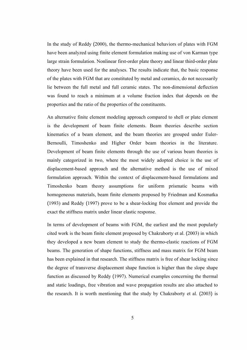
In terms of development of beams with FGM, the earliest and the most popularly

cited work is the beam finite element proposed by Chakraborty et al. (2003) in which

they developed a new beam element to study the thermo-elastic reactions of FGM

beams. The generation of shape functions, stiffness and mass matrix for FGM beam

has been explained in that research. The stiffness matrix is free of shear locking since

the degree of transverse displacement shape function is higher than the slope shape

function as discussed by Reddy (1997). Numerical examples concerning the thermal

and static loadings, free vibration and wave propagation results are also attached to

the research. It is worth mentioning that the study by Chakraborty et al. (2003) is

6

popularly cited in the literature and is considered as a benchmark formulation for

FGM beams.

Stability analysis of functionally graded beams has been carried out in the study by

Mohanty et al. (2011) through the use of the finite element proposed by Chakraborty

et al. (2003). In that work, the researchers examined the dynamic stability of

functionally graded ordinary beams and functionally graded sandwich beams on

Winkler’s elastic foundation. Functionally graded ordinary (FGO) beams consist of

first material 100% at top of the section; second material 100% at the bottom of the

section with a transition zone from topmost to bottommost of the section. Whereas,

in functionally graded sandwich (FGSW) beams; the transition zone appears as a

core material between first material at the top with a finite thickness and second

material at the bottom likewise. In Figure 2 section (A) represents the functionally

graded sandwich beam and section (B) represents the functionally graded ordinary

beam in which the transition is through the whole section. In that work, it is

concluded that for a functionally graded sandwich beam; if the materials vary with

respect to the power law the beam becomes less stable as the thickness of the FGM

core increases. In the other case, as the materials vary according to exponential law,

an increase in the thickness of the FGM core improves the stability of the beam.

In study by Hemmatnezhad et al. (2013), large amplitude free vibration analysis,

imposing von Karman type of large strain, of beams with functionally graded

materials, is realized. The finite beam element formulation for FGM, proposed by

Chakraborty et al. (2003) has been used in that study, as well. The results obtained

from numerical simulations are compared with theory of elasticity solutions available

in the literature.

Besides the development and use of displacement-based finite elements, it is also

possible to formulate mixed formulation finite elements for the analysis of FGM

beams. In the literature, it appears that there is no such element proposed and used

for the analysis of beams with FGM. It is furthermore worth to mention that inelastic

analysis of FGM members has not been undertaken in the context of beam finite

elements.

model for

materials h

finite elem

parameter

this requir

for the ine

Figu

For the sa

based and

Since the

initial forc

in order t

Displacem

virtual dis

energy. In

formulatio

and the sa

weak satis

the fields l

In a study

r metallic m

have been p

ments have

rs of FGM r

res significa

elastic analy

ure 2 Varia

ake of comp

d mixed for

proposed b

ce-based ele

to point ou

ment-based

splacements

n this approa

on approach

atisfaction o

sfaction of v

listed in the

y by Boccia

materials an

proposed fo

been used

requires bot

ant amount

ysis of FGM

ation of mat

pleteness of

rmulation b

beam elem

ement propo

ut also the

elements a

s or more g

ach, displac

hes, stress a

of the equa

variational p

e table, refer

7

arelli et al.

nd Drucker-

or the analy

d for model

th experime

of effort. In

M beams.

terial prop

f literature s

beam finite

ment actually

osed in the l

differences

are formula

generally c

cement field

and strain f

ations are w

principles a

r to the wor

(2008) the

-Prager plas

ysis of FGM

ling FGM.

ental studies

n this thesis

erties on th

survey, the

elements

y bases on

literature, su

of the ele

ated within

called as pr

ds are the in

fields are al

weakened. A

are listed in

rk by Saritas

e use of Vo

sticity mode

M members.

Identificati

s and analyt

, an effort i

he depth of

developmen

is also pres

the same

uch a prese

ement propo

n the conte

rinciple of

ndependent

lso brought

A summary

Table 1. Fo

s and Soyda

on Mises p

el for ceram

In that stud

ion of the

tical validat

s also demo

f FGM beam

nt and use o

sented in th

assumption

ntation is n

osed in thi

ext of prin

minimum p

variables. I

into the fu

y of the str

or the descri

as (2012).

plasticity

mic type

dy, solid

material

tion, and

onstrated

ms

of force-

his part.

ns of the

ecessary

s thesis.

nciple of

potential

In mixed

unctional

rong and

iption of

8

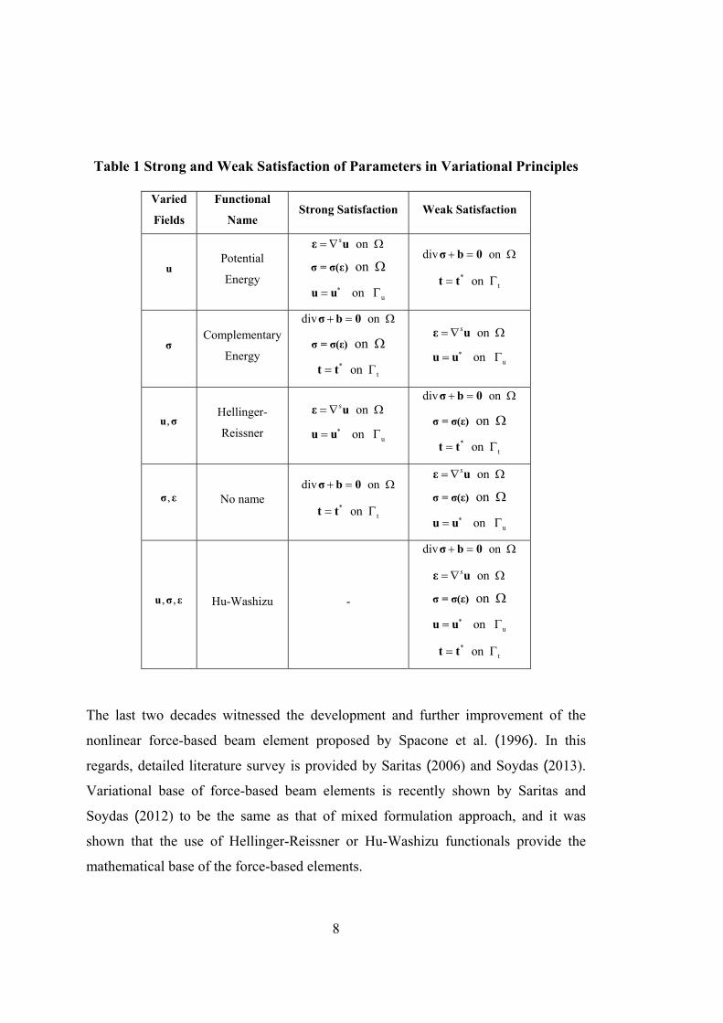
Table 1 Strong and Weak Satisfaction of Parameters in Variational Principles

Varied

Fields

Functional

Name Strong Satisfaction Weak Satisfaction

u Potential

Energy

on s ε u

on σ = σ(ε)

u on u u

div on σ b 0 *

t on t t

σ Complementary

Energy

div on σ b 0

on σ = σ(ε) *

t on t t

on s ε u

u on u u

,u σ Hellinger-

Reissner

on s ε u

u on u u

div on σ b 0

on σ = σ(ε) *

t on t t

,σ ε No name div on σ b 0

*t on t t

on s ε u

on σ = σ(ε)

u on u u

, ,u σ ε Hu-Washizu -

div on σ b 0

on s ε u

on σ = σ(ε)

u on u u *

t on t t

The last two decades witnessed the development and further improvement of the

nonlinear force-based beam element proposed by Spacone et al. (1996). In this

regards, detailed literature survey is provided by Saritas (2006) and Soydas (2013).

Variational base of force-based beam elements is recently shown by Saritas and

Soydas (2012) to be the same as that of mixed formulation approach, and it was

shown that the use of Hellinger-Reissner or Hu-Washizu functionals provide the

mathematical base of the force-based elements.

9

Initial and the most widely cited work in terms of development of a nonlinear force-

based beam finite element was first documented in detail by Spacone et al. (1996).

The element sets forward to the consistent numerical implementation of the element

state determination in the context of a standard FEM package. For the displacement-

based finite elements the iterative process depends on the residual forces whereas for

the proposed element, the procedure is based on the residual deformations.

In a recent study by Soydas and Saritas (2013), an accurate nonlinear 3d beam finite

element is proposed for inelastic analysis of solid and hollow circular sections. The

element is based on Hu-Washizu functional and axial force, shear forces, bending

moments about both axes and torsional moment is coupled through the use of 3d

material models and fiber discretization of the section and the use of several

monitoring sections along element length. The element proposed in that work proved

to be very effective in capturing the behavior of long and short members that are

loaded and restrained in various fashions.

1.3. OBJECTIVES AND SCOPE OF THESIS

In this thesis, the development of a force-based beam element for the analysis of

functionally graded materials is considered. The beam element that is developed in

this thesis is based on the use of force interpolation functions instead of the

approximation of displacement field. The response of the proposed element is

calculated through aggregation of responses of several monitoring sections. Section

response is calculated by subdividing the depth of a monitoring section into several

layers and by aggregating the material response on the layers. Since the formulation

of the element bases on force interpolation functions that are accurate under both

elastic and inelastic material response, the proposed element provides robust and

accurate linear and nonlinear analysis of FGM beams with respect to displacement-

based approach. The formulated element is compared with a previously developed

displacement-based beam finite element by Chakraborty et al. (2003).

10

For inelastic analysis, von Mises plasticity model with isotropic and kinematic

hardening parameters is assigned for both materials for simplicity. A simply

supported pin-pin FGM beam is divided into different numbers of elements (both

force-based and displacement-based beam elements), and the simply supported

system is exposed to support vertical displacement from the mid-span. The results

indicate the accuracy and robustness of the proposed element over the displacement-

based element in terms of global level response as well as local measures such as

forces and stresses.

The second effort in this thesis focuses on the vibration characteristics of the

proposed beam element with FGM. Consistent mass matrix for the force-based

element is implemented for the validation of the vibration modes and shapes

obtained from this element. For this effort, benchmark problems are both analyzed

with proposed beam element and with 3d solid elements in ANSYS. The results

indicate that proposed element provides not only accurate results in lower modes but

also in higher modes of vibration.

1.4. ORGANIZATION OF THESIS

In the second chapter force-deformation relations of proposed beam element will be

presented and some principal beam theories and their section kinematics will be

mentioned. Then, the implementation of force-based elements into a nonlinear FEM

package and the convergence rate of the Newton–Raphson iteration procedure will

be discussed and derivation of the stiffness matrix and the consistent mass matrix for

the proposed force-based beam element will be presented.

In the third chapter; a previously developed displacement-based beam element for

FGM will be provided for the sake of completeness of the thesis work. The

formulations for the element will be discussed in detail, where it was observed that

some of the coefficients presented in the original work required correction.

11

In the fourth chapter; the material model, which is selected to mimic the behavior of

materials in the FGM section, has been formulated. The radial return mapping

algorithm for the von Mises plasticity has been presented.

In the fifth chapter numerical analyses for the proposed beam element will be held

out. Firstly, non-linear analysis will be realized for the force-based element and then

the results will be compared with the displacement-based element. Secondly, modal

analyses will be realized for the proposed force-based finite beam element. The

modal shapes and natural frequencies will be compared with the results obtained

from ANSYS.

Finally in the sixth chapter, conclusion and recommendations for further studies will

be documented.

12

13

CHAPTER 2

FORCE-BASED ELEMENT FOR FGM BEAMS

In this chapter, first, force-deformation relations of frame element will be clarified,

and then some principal beam theories and their section kinematics will be

mentioned. Thirdly, the implementation of force-based elements into a nonlinear

FEM package and the convergence rate of the Newton–Raphson iteration procedure

will be discussed. Development of the proposed beam element is done in a basic

system where rigid body modes are eliminated. For this reason, conversion of the

beam response from the basic system to the complete system is cast in this chapter

after the formulation of the beam element in the basic system. Finally, derivation of

the consistent mass matrix for the force-based beam element is explained.

2.1. FORCE-DEFORMATION RELATIONS OF FRAME ELEMENT

WITH SHEAR DEFORMATIONS (TIMOSHENKO BEAM THEORY)

In this subtopic the element force relations, force shape functions and the derivation

of section flexibility and stiffness matrices will be clarified.

Figure 3 Simply supported basic system for force-based beam element

14

Figure 3 shows the element end forces of a simply supported (pin-pin) basic system.

In the absence of element loads the axial force and shear force distribution is

constant and moment distribution is linear with respect to x-axis.

Figure 4 Nodal end forces and beam statics for force-based beam

From Figure 4 the axial force, shear force and moment equations can be derived

through simple statics knowledge as follows

1

2 3

2 3

( )

( ) ( 1) ( )

( ) ( ) /

N x q

x xM x q q

L LV x q q L

(2.1)

Equation (2.1) can be written in matrix notation as

( ) 1 0 0 1

( ) ( ) 0 / 1 / 2 ( )

( ) 0 1/ 1/ 3

N x q

s x M x x L x L q b x q

V x L L q

(2.2)

In (2.2), the section forces, force interpolation (equilibrium) matrix and element

force vector will be shown as ( )s x

, ( )b x

and q

, respectively.

Now if the principle of virtual forces is used, the following equality can be written.

0

( ) ( )L

T Tq v s x e x dx (2.3)

15

In (2.3), ( )e x

represent the section deformations, where the components of this vector

will be mentioned later in this chapter.

The same interpolation functions have been selected for the force field and the virtual

force field, thus

( ) ( )T T Ts x q b x

(2.4)

Inserting (2.4) into (2.3) we obtain the element deformation vector v

in the basic

system as follows

0

( ) ( )L

Tv b x e x dx (2.5)

Making use of the chain rule, flexibility matrix of the beam element is obtained.

0 ( )( )( )

( ) ( )L

Ts

s xe xqs x

vf b x f b x dx

q

(2.6)

In (2.6) f

is the element flexibility matrix. The terms ( )

( )

e x

s x

and ( )s x

q

are written

as sf

and ( )b x

, respectively. The matrix sf

, so called section flexibility matrix can

be computed from the inverse of the section stiffness matrix through the relation

1s sf k

. Section stiffness matrix sk

will be introduced in the next subtopic.

2.2. SECTION KINEMATICS

In this part two beam theories and their section characteristics will be mentioned.

First the Euler-Bernoulli beam theory will be represented, where the plane sections

remain plane and the angle between the normal of the section and tangent to the

deformed axis of the beam is zero, thus no shear deformation takes place in this

16

beam theory. The second one is, Timoshenko’s beam theory, where in this theory

plane sections remain plane likewise, but the angle between the normal of section

and the tangent to the deformed axis of the beam is not necessarily equal to zero.

According to Timoshenko’s beam theory the beam element can exhibit shear

deformations.

There are also other beam theories where the plane sections do not have to remain

plane, so called higher order beam theories. A discussion of higher order beam

theories is available in the paper by Reddy (1997).

2.2.1. Euler-Bernoulli Beam Theory

Figure 5 shows the cross section of a beam element. An arbitrary point P is described

on the cross section.

Figure 5 Arbitrary cross-section for a solid beam element

Assuming that Euler-Bernoulli beam theory assumptions hold, we can only calculate

a non-zero strain value that is the normal strain, and it is expressed as follows

, , ( ) ( ) ( )a z yx y z x y x z x (2.7)

Since our analysis is in 2d, we do not seek for moments around y axis; thus curvature

about y axis is not taken into account, and Equation (2.7) can be simplified as

( ) ( )x a x y x (2.8)

17

Hereupon, the curvature about z axis is simply denoted with . We can show (2.8)

in vector notation as

( )1

( )a

x

xy

x

(2.9)

2.2.2. Timoshenko’s Beam Theory

The difference between Timoshenko and Euler – Bernoulli beam theories is that, the

plane sections after deformation will not remain normal to deformed axis of the

beam; thus another deformation variable on the section is introduced to represent

the angle difference between the normal to the section and the tangent to the

deformed axis of the beam.

Rest of the formulations in this chapter will constitute utilization of the Timoshenko

beam theory section kinematics, where the strains on the section of a 2d beam

element can be written as follows

1 0

0 0 1

ax

xy

y

(2.10)

or

( )x

xysa e x

(2.11)

where is the shear deformation of section on the x-y plane in (2.10), sa

is the 2x3

compatibility matrix and e

is the 3x1 section deformation vector in (2.11).

Now we will establish the relation between section forces and section deformations.

( ) T

A

ss x a dA (2.12)

18

where

0

0x x

xy xy

E

G

(2.13)

( )

( ) ( )

( )

N x

s x M x

V x

(2.14)

( )s x

is the vector of section forces, where N, M and V are axial force through x axis ,

moment about z axis and shear force along y axis, respectively.

Substituting (2.11) and (2.13) into (2.12) we get

0( ) ( )

0T

s s

A

Es x a a dA e x

G

(2.15)

Where the term in brackets is sk

which is called the section stiffness matrix. If the

material properties do not vary through the section depth, section stiffness matrix can

be written as follows

2

0 0

0 0

0 0 0 0s

A

E yE EA EQ

k yE y E dA EQ EI

G GA

(2.16)

Where, I is the moment of inertia about the bending axis, Q is the first moment of the

area about the bending axis, and if the bending axis matches with the geometric

centroid then Q is equal to zero. In above equation, GA term is usually corrected for

the presence of non-uniform distribution of shear over the section, and sGA is

substituted instead of GA.

Since we are dealing with FGM; Young modulus (E) and shear modulus (G) vary

through the depth of the section. So, the modulus matrix cannot be taken outside the

integral. For FGM sections sk

must be computed as follows

19

( ) 0

0 ( )T

s

A

s s

E yk a a dA

G y

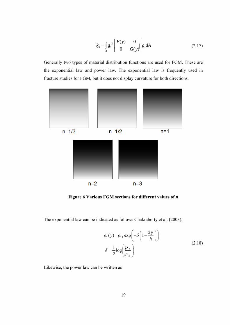
(2.17)

Generally two types of material distribution functions are used for FGM. These are

the exponential law and power law. The exponential law is frequently used in

fracture studies for FGM, but it does not display curvature for both directions.

Figure 6 Various FGM sections for different values of n

The exponential law can be indicated as follows Chakraborty et al. (2003).

2( ) exp 1

1log

2

t

t

b

yy

h

(2.18)

Likewise, the power law can be written as

20

1

( ) ( )2t b b

ny

yh

(2.19)

Here ( )y represents the material properties such as elastic modulus, shear modulus,

thermal expansion coefficient, mass density etc. t and b stand for the topmost

and bottommost materials, respectively. It is suggested that the power coefficient n

can be taken between 1/3 and 3. Otherwise, FGM would contain too much of one

phase (1/3 or 3 contributes to %75 of total volume) (refer to the work by Nakamura

et al. (2000)).

Figure 6 and Figure 7 show the material distribution for several FGM sections with

different power law coefficients (n).

Figure 7 Distribution of ingredients for different values of n

21

2.3. TRANSFORMATION BETWEEN BASIC SYSTEM AND COMPLETE

SYSTEM

In this part, conversion from simply supported (pin-pin) basic system to the complete

system will be discussed. In the basic system, rigid body modes of displacements are

eliminated, thus there are only the element deformations.

In 2d case, there are three element deformations, namely the axial deformation and

the two end rotations for the simply supported basic system. We can also choose

cantilever basic system as an alternative, and in that case assuming the left end fixed,

there will be one axial deformation, one transverse displacement and one rotation as

element deformations existing on the right end of the element.

In the complete system, the element has two nodes and at each node there are 3

degrees of freedom, i.e. the translations along and transverse to the element and the

rotation at that node.

The necessity of the transformation between the basic system and the complete

system stems from the formulation of the force-based element in the basic system

and the fact that the FEM program will provide nodal displacements in the complete

system.

From Figure 8, making use of the small deformation theory, the compatibility

equations between element deformations and nodal displacements are derived as

follows:

1 4 1

2 3

3 6

v u u

v u

v u

(2.20)

where 5 2( )u u

L

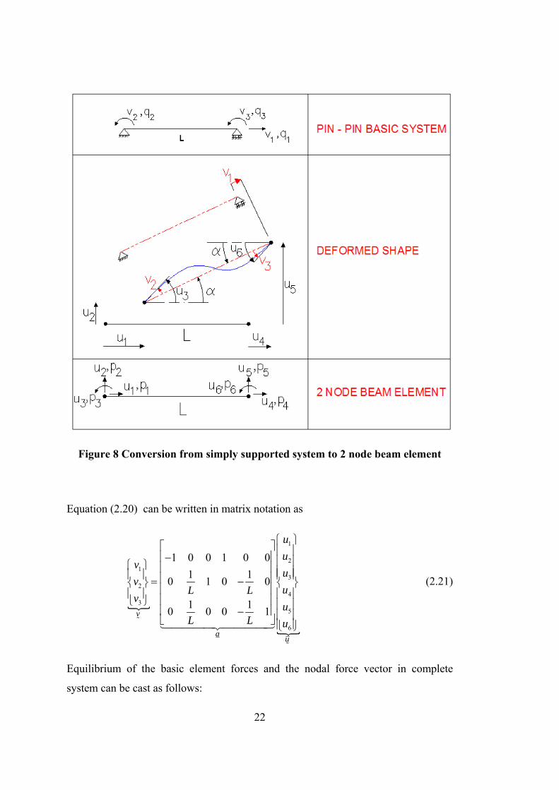
22

Figure 8 Conversion from simply supported system to 2 node beam element

Equation (2.20) can be written in matrix notation as

1

21

32

43

5

6

1 0 0 1 0 0

1 10 1 0 0

1 10 0 0 1v

au

u

uv

uv

uL Lv

uL L u

(2.21)

Equilibrium of the basic element forces and the nodal force vector in complete

system can be cast as follows:

23

1

21

32

43

5

6

1 0 0

1 10

0 1 0

1 0 0

1 10

0 0 1T

q

p

a

p

p L L qp

qp

qp

L Lp

(2.22)

Given that basic element forces are related to the basic element deformations with

the relation q kv

, we can substitute (2.21) in (2.22) to get

elp k u

(2.23)

where Telk a ka

is the element stiffness matrix in complete system for the two node

beam element. This stiffness matrix is actually now calculated in the element local

coordinate system. Further transformation can be easily achieved by rotation to the

global coordinate system in order to consider the angles between the local

coordinates x, y and z and the global coordinates X, Y and Z. In depth discussion of

these transformations is available in Filippou and Fenves (2004) for 2d case and

Soydas (2013) for 3d case.

2.4. STATE DETERMINATION OF FORCE-BASED ELEMENT

Implementation of the force-based element is sought in standard finite element

software that is based on displacement method of analysis. In such a solution

platform, displacements are incremented iteratively in order to achieve convergence

to the applied loads. Since the force-based element requires the input of element

forces and its output is element deformations, an element state determination

procedure is necessary for the force-based element to be a part of the solution

strategies of displacement-based solutions.

24

The general procedure for handling nonlinearity in displacement-based finite element

solution platform can be summarized as follows. Finite element program solves the

nonlinear system of equations between applied forces appP

and resisting forces rP

.

( ) 0app rP P u

(2.24)

Since the equation is nonlinear, the system must be linearized in order find the

correct displacements that satisfy above equation. By using Taylor’s series expansion

about an initial guess, an incremental iterative solution for global nodal

displacements is obtained as given in the next equation, and this iterative process is

also named as Newton-Raphson method.

1

( ){ ( )} 0

{ ( )}

r iapp r i i

i i app r i

iK

P uP P u U

U

U K P P u

(2.25)

An initial guess for global nodal displacements can be taken as 0 0U

for the start of

analysis or the last state of converged nodal displacements.

After calculation of each increment, global nodal displacements U

are updated and

sent to each element with the purpose of receiving back element forces and stiffness.

Since the force-based element actually provides output of element deformations, then

the element state determination can be established by imposing the nodal

displacements calculated from Equations (2.21) and (2.25). We denote the imposed

element deformations received from the finite element program as (v

). Imposed

deformations should match with the state of the force-based element, and this

compatibility statement can be written as follows:

( ) 0v v q

(2.26)

25

The term ( )v q

in (2.26) is the response of the force-based element, and under general

case the response of the element is nonlinear and requires linearization as written in

the next equation:

0

0

0 0( ) ( ) 0q q q

f

vv v q q q

q

(2.27)

1

iiq f v v

(2.28)

1i iq q q

(2.29)

In (2.28) the term inverse of section flexibility matrix 1

isf

, that is equal to section

stiffness matrix sk

, can be computed from (2.17).

With the calculation of new updates for basic element forces from Equation (2.29),

new values of section forces can be obtained by the use of Equation (2.2), i.e.

( ) ( )s x b x q

. Since the section state determination requires the input of section

deformations but not the section forces, then one more effort is necessary to match

the imposed section forces calculated from ( ) ( )s x b x q

with ( )s e

. For this effort,

the imposed section forces are denoted with a hat value to signify the imposed

quantity, the equality to be satisfied is written as follows:

( ) 0s s e

(2.30)

The section deformations must be compatible with element end forces. The term

( )s e

will be linearized as follows

26

0

0

0 0( ) ( ) 0

s

e e e

k

ss s e e e

e

(2.31)

Inserting ( )s b x q

into (2.31), we get

1( ) ( )i

s ie k b x q s e

(2.32)

1i ie e e

(2.33)

The element deformations will be computed as given in Equation (2.5) and with the

new values of section deformations computed from Equation (2.33), we obtain

1 1

0

( ) ( )L

Ti iv b x e x dx

(2.34)

Equation (2.32) requires the calculation of section stiffness matrix sk

. The numerical

computation process of sk

for beams consisting of only one material can be

summarized as follows. The material subroutine reads the section deformations ( 1ie

)

and history variables (in case of hardening) at each layer of the beam section and at

each integration point along the length of the beam as input, then it takes out the

consistent tangent modulus and stresses as output variables. The consistent tangent

modulus and stresses at each layer of the beam’s cross section are transferred into a

numerical integration process to acquire the section stiffness matrix and section

forces as written in the following equation:

Ts

A

s sk a a dA

(2.35)

27

For beams with FGM, the section deformations and history variables are sent to two

different material subroutines separately and then these two separate material outputs

are added in accordance with their weighted material ratio at the layer.

With the calculation of section stiffness matrix, the element flexibility matrices ( f

)

and element stiffness matrices (k

) will also be updated with the use of following

equations:

1 1

01 1 1

( ) ( )

[ ]

Li T i

i i

sf b x f b x dx

k f

(2.36)

where 11 1i i

ssf k

is the section flexibility matrix corresponding to 1( )ie x

each

section deformations.

The convergence check is handled at the global level through the satisfaction of

equilibrium equations within a tolerance, i.e. ( )app r iP P u TOLERANCE

, the

iteration stops.

2.5. THE CONVERGENCE RATE OF NEWTON–RAPHSON METHOD

Newton–Raphson iteration procedure is utilized for the solution strategy of the

nonlinear system of equations. The stiffness matrix is updated and its inverse is

calculated at each iteration. As exhausting as it may seem in terms of computational

cost, the convergence rate of this method is quite powerful.

The convergence rate of the Newton–Raphson method can be proven as follows.

First the Taylor series will be portrayed

2 (3) 3

Higher Order Terms (H.O.T.)

'( )( ) ''( )( ) ( )( )( ) ( ) ... 0

1! 2! 3!n n n n n n

n

f x x f x x f x xf f x

(2.37)

28

Making use of the mean value theorem, one can prove the existence of such point

x that satisfies (2.37) in the following form

2'( )( ) ''( )( )

( ) ( ) 01! 2!

n n nn

f x x f xf f x

(2.38)

In (2.38), 2''( )( )

2!nf x

represents the H.O.T. (higher order terms).

The iteration steps of Newton–Raphson method is visualized in Figure 9

Figure 9 Visualization of Newton–Raphson iterations

Following relation can be comprised from Figure 9

1

( )

'( )n

n nn

f xx x

f x (2.39)

After dividing (2.38) with '( )nf x and rearranging the terms, the following equation

is obtained

2( ) ''( )( )

0'( ) 2 '( )

n nn

n n

f x f xx

f x f x

(2.40)

29

Inserting (2.39) into (2.40) leads us to the final relation between the error terms of

successive iterations.

21

1

''( )( )

2 '( )n nn

nn

fx x

f x

(2.41)

Taking the absolute of right and left sides, we can write

2

1

''( )

2 '( )n nn

f

f x

(2.42)

Since there is a quadratic relation between the errors of successive iterations, the

convergence rate of Newton–Raphson iteration method is quadratic provided that the

tangent to the function is accurately calculated.

2.6. FORCE-BASED CONSISTENT MASS MATRIX

In this thesis, mass matrix of the proposed element for FGM beams is obtained in a

consistent manner with the formulation of the element. Since the proposed element

does not require the use of displacement interpolation functions, it is necessary to

derive the displacement field along the length of the beam in a consistent way with

the force-based formulation. This can actually be obtained in a simple fashion with

unit dummy load method, i.e. with the use of principle of virtual forces approach as

done in the derivation of the element in Section 2.1. Such an approach was proposed

by Molins et al. (1998) and successfully implemented and used recently by Soydas

(2013). With this alternative derivation of consistent mass matrix, we can obtain the

mass matrix of any type of beam element that is uniform or tapered and with

homogeneous or heterogeneous material distribution.

Derivation of the mass matrix within force-based approach relies on the use of

cantilever basic system due to its simplicity in establishing the displacement field.

For the cantilever basic system, the basic element forces are axial force and

30

transverse (shear) force and moment values at the right node, while the left node is

fixed. Actually these three basic forces exactly match with the element end forces for

the complete system as well. Denoting the basic forces of cantilever system as cq

,

we can calculate the section forces as follows:

( )

( ) ( ) ( , )

( )c c

N x

s x V x b x L q

M x

(2.43)

Where the section forces are arranged as given above, and the force interpolation

matrix for the cantilever basic system is

1 0 0

( , ) 0 1 0

0 ( ) 1cb x L

L x

(2.44)

The section mass and stiffness matrices are calculated as:

T( ) ( )s s s

A

m x a y a dA (2.45)

T ( ) 0( )

0 ( )s s s

A

E yk x a a dA

G y

(2.46)

where sa

the section compatibility matrix previously introduced in Equations (2.10)

and (2.11) is rearranged as follows:

1 0

0 1 0s

ya

(2.47)

Mass matrix of the force-based element is written in a 6×6 dimension, i.e. in the

complete system with 3 degrees of freedom per each end node, as follows:

11 12

21 22el

m mm

m m

(2.48)

31

Where the components of element mass matrix are calculated from sub-matrices

-1 T 1 T -122

0

( , ) ( ) ( , ) ( ) ( )L L

c c s c s cp c

x

m f b x L k x b x m f f d dx

(2.49)

-1 T 1 T T -1 T21

0

( , ) ( ) ( , ) ( ) (0, ) ( ) (0, )L L

c c s c s c cp c c

x

m f b x L k x b x m b f f b L d dx

(2.50)

-112 21 22

0

(0, ) (0, ) ( ) ( )L

c c s cp cm m b L m b x m x f x f dx (2.51)

T -1 T11 21

0

(0, ) (0, ) ( ) (0, ) ( ) (0, )L

c c s c cp c cm b L m b x m x b x f x f b L dx (2.52)

In above equations, element flexibility matrix for the cantilever system is denoted as

cf

, and it is calculated as follows:

T -1

0

( , ) ( ) ( , )L

c c s cf b x L k x b x L dx (2.53)

And the partial flexibility matrix cpf of the cantilever system is given as:

T -1

0

( ) ( , ) ( ) ( , )x

cp c s cf x b x k x b x d (2.54)

Force-based consistent mass matrix for prismatic beams with FGM obtained from

Equations (2.48) to (2.53) are compared with the mass matrix of the displacement-

based element proposed by Chakraborty et al. (2003) that is presented in the next

chapter, and they are observed to be giving the same matrix for uniform prismatic

FGM beams. However, in the case when the beam is tapered, then the displacement-

based approach will result in an approximation, while the proposed approach will

still give the exact consistent mass matrix for FGM beams.

32

A

In this cha

al. (2003)

not been c

Also, duri

shape fun

beam elem

presentatio

3.1. FO

In Chakra

transverse

A DISPLAC

apter, a prev

will be dis

clearly state

ing this inv

nctions appe

ment will

on of this el

ORMULAT

Figure 1

aborty et al

e displaceme

CEMENT-

viously dev

cussed. Som

d in Chakra

vestigation,

ears to be

be used i

lement is ju

TION OF D

10 Coordina

l. (2003), c

ent fields ar

33

CHAPT

-BASED EL

veloped beam

me of the fo

aborty et al.

it has also

represented

in the num

ustified for t

DISPLACE

ate system

onsidering

re expressed

3

ER 3

LEMENT

m finite ele

ormulations

(2003) are

been detec

d incorrectl

merical exa

the sake of c

EMENT-BA

for the fini

Timoshenk

d as,

FOR FGM

ement for FG

and deriva

presented i

cted that a

y. Since th

amples and

completene

ASED ELE

ite element

ko beam th

M BEAMS

GM Chakra

ation steps th

in detail.

coefficient

he mentione

d verificatio

ss.

EMENT

t model

eory, the a

aborty et

hat have

used in

ed finite

ons, the

axial and

34

( , , , ) ( , ) ( , )

( , , , ) ( , )

U x y z t u x t y x t

W x y z t w x t

(3.1)

The strains are expressed as

, ,

,

x x x

xy x

Uu y

xU W

wy x

(3.2)

Where (.),x represents differentiation with respect to x-axis.

The relation between stress and strain is expressed as

( ) 0

0 ( )x x

xy xy

E y

G y

(3.3)

The strain energy (S) and kinetic energy (T) are written as

0

1( )

2

L

x x xy xy

A

S dAdx (3.4)

2 2

0

1( )( )

2

L

A

T y U W dAdx (3.5)

Where (.) represents the time derivative. ( )y , L and A are density, length and the

area of the cross section. Applying Hamilton’s principle, the following equations of

motion are obtained. The implementation of Hamilton’s principle is explained in

Appendix.

0 1 11 11

0 55

2 1 11 11 55

: , , 0

: ( , , ) 0

: , , ( , )

xx xx

xx x

xx xx x

u I u I A u B

w I w A w

I I u B u D A w

(3.6)

Where

35

211 11 11

55

20 1 2

1 ( )

( )

1 ( )

A

A

A

A B D y y E y dA

A G y dA

I I I y y y dA

(3.7)

The interpolation functions for , ,u w are selected for the element to be giving a

shear-locking free element.

In case of assigning interpolation functions improperly for the vertical translation and

slope, the phenomenon called shear locking occurs. Especially, if linear interpolation

functions are assigned for both vertical translation and slope, then the beam element

behaves very stiff for larger values of length to depth ratio. To deal with this

phenomenon, one should use higher order interpolation functions for vertical

translation than slope.

Since the order of interpolation function for vertical translation ( w) is higher than the

order of the interpolation function for the slope ( ) as discussed by Reddy (1997).

21 2 3

2 34 5 6 7

28 9 10

u c c x c x

w c c x c x c x

c c x c x

(3.8)

The term 11B and 1I is zero for homogenous sections. Completing the following

formulations with the specified shape in such case will end up with the stiffness

matrix in Reddy (1997), i.e. the Interdependent Interpolation Element for

Timoshenko’s beam theory. This so called beam element is been utilized as the

default frame element for some popular FEM packages like SAP2000.

Equation (3.8) is substituted into the static part of (3.6). The static part of (3.6) is

obtained by eliminating the terms with time derivatives, thus the governing partial

differential equation is transformed into a system of ordinary differential equations.

The static part of (3.6) can be shown as

36

11 11

55

11 11 55

: , , 0.................(3.13.1)

: ( , , ) 0.................(3.13.2)

: , , ( , )....(3.13.3)

xx xx

xx x

xx xx x

u A u B

w A w

B u D A w

(3.9)

Also

32

5 6 7

6 7

9 10

10

, 2

, 2 3

, 2 6

, 2

, 2

xx

x

xx

x

xx

u c

w c c x c x

w c c x

c c

c

(3.10)

Substituting (3.10) into (3.9)1

113 10

11

Bc c

A (3.11)

Substituting (3.10) into (3.9)2

6 7 9 102 6 2 0c c x c c x (3.12)

From (3.12)

107

96

3

2

cc

cc

(3.13)

Substituting (3.10) into (3.9)2 and using (3.11)

2 211 3 11 10 55 5 6 7 8 9 10

11 3 11 10 55 5 8

211

10 11 10 55 5 811

10 5 8

3 5 8

2 2 ( 2 3 0

2 2 ( ) 0

2 2 ( ) 0

( ) / 2

( ) / 2

B c D c A c c x c x c c x c x

B c D c A c c

Bc D c A c c

A

c c c

c c c

(3.14)

37

Where 11 552

11 11 11( )

A A

B D A

and 11 55

211 11 11( )

B A

B D A

Using (3.13) and (3.14) interpolation functions can be rewritten as

21 2 5 8

2 34 5 9 5 8

28 9 5 8

1( )

21 1

( )2 61

( )2

u c c x c c x

w c c x c x c c x

c c x c c x

(3.15)

In matrix form

1 2 4 5 8 9

{ } [ ( )]{ }

{ } { , , , , , }

u

u w N x a

a c c c c c c

(3.16)

A relation can be formed between column vector { }a and nodal displacements by

using boundary conditions for each node, (at x=0 and x=L)

1

1

(0)[ ]

( )

ˆ{ } [ ] { }

ˆ{ } [ ]{ }

NG

N L

u G a

a G u

(3.17)

Where[ ( )]N x , 1[ ]G and [ ]G are

2 2

3 3 2

2 2

1 11 0 0

2 21 1 1

[ ( )] 0 0 16 6 2

1 10 0 0 1

2 2

x x x

N x x x x x

x x x

(3.18)

38

2 2

1

3 3 2

2 2

1 0 0 0 0 0

0 0 1 0 0 0

0 0 0 0 1 0

1 11 0 0[ ] 2 2

1 1 10 0 1

6 6 21 1

0 0 0 12 2

L L LG

L L L L

L L L

(3.19)

2 2 2 2

2

3 2 3 2

2 2

2 3 2 3

1 0 0 0 0 0

1 6 3 1 6 3

12 12 12 12

0 1 0 0 0 0

[ ] 12 6 12 60 0

12 12 12 12

0 0 1 0 0 0

6 (4 12) 6 (2 12)0 0

12 12 12 12

L L

L L L L L L

G L

L L L L L L

L L

L L L L L L

(3.20)

1 1 1 2 2 2ˆ{ }T

u u w u w is the vector of nodal displacements of the element.

The exact shape functions can be derived by multiplying [ ( )]N x and [ ]G

ˆ ˆ{ } [ ( )]{ } [ ( )][ ]{ } [ ( )]{ }

[ ( )] [ ( )][ ]

u

u w N x a N x G u x u

x N x G

(3.21)

[ ( )] ( ) ( ) ( )T

u wx x x x is a 3x6 matrix containing the exact shape

functions for axial, transverse and rotational degrees of freedom.

Element force members (axial, shear and moment) can be expressed as

39

x xx

A

x xx

A

x xx

A

N dA

V dA

M y dA

(3.22)

Imposing (3.2) and (3.3); (3.22) can be written as

11 11

55

11 11

, ,

( , )

, ,

x x x

x x

x x x

N A u B

V A w

M B u D

(3.23)

From (3.23) element force vector can be associated with vector { }a in matrix form as

{ } [ ]{ }F G a (3.24)

where [ ]G and { }F are

11 11

55 55

11 11

11 11

55 55

11 11 11 11 11 11

0 0 0 0

0 0 0 0

0 0 0 0[ ]

0 0 0 0

0 0 0 0

0 0

A B

A A

B DG

A B

A A

B B D L D B L D

(3.25)

{ } [ (0) (0) (0) ( ) ( ) ( )]x x x x x xF N V M N L V L M L (3.26)

The stiffness matrix can be evaluated by substituting (3.17) into (3.24)

ˆ ˆ{ } [ ][ ]{ } [ ]{ }F G G u K u (3.27)

[ ( )]x (exact shape functions) and [ ]K (stiffness matrix) are

40

3 3 2

3 2 2 2 3 2

2

2 2

1 0 0

( 12 12 2 3 )6 ( 1) 6 ( 1)

( 6 6 2 ) (3 12 4 12 )3 ( 1)

[ ( )]

0 0

( 12 2 3 )6 ( 1) 6 ( 1)

( 6 6 )3 ( 1)

x

L

x L L x x x L xx x

L L L

x x L L x x L xL x L L L x L xxL

L L Lx

x

L

x x x xL xx x

L L L

x x L x L xL x xxL

L L

2(3 2 12)

T

xL L

L

(3.28)

11 11 11 11

55 55

55 55

11 11

11 55 55 11 55 55

11 11 11 11

55 55

55 55

11 11

11 55 55 11 55 55

/ 0 / / 0 /

12 120 6 0 6

/ 6 3 / 6 3

[ ]/ 0 / / 0 /

12 120 6 0 6

/ 6 3 / 6 3

A L B L A L B L

A AA A

L L

D DB L A A L B L A A L

L LK

A L B L A L B L

A AA A

L L

D DB L A A L B L A A L

L L

(3.29)

where 2

1

12 L

3.2. THE CONSISTENT MASS MATRIX

The consistent mass matrix is described as summation of four sub-matrices as given

by Chakraborty et al. (2003).

u w uM MM M M (3.30)

41

uM , wM and M stand for the contributions of axial (u), translational ( w )

and slope ( ) degree of freedoms. uM represents the coupling between axial and

slope degree of freedoms.

The components of consistent mass matrix are figured as follows

0

0

0

0

2

0

1

0

( )

( )

( )

( )

LT

u u

LT

w w

LT

LTT

u u

u

w

u

I dx

I dx

I dx

M I dx

M

M

M

(3.31)

For homogenous sections; since 1I is zero, it can be indicated from (3.31) that the

term uM yields zero.

42

43

CHAPTER 4

MODELING INELASTIC BEHAVIOR OF FGM BEAMS

In this chapter, firstly the von Mises plasticity and its yield criteria will be presented.

Secondly, evolution equations will be derived for the von Mises model with linear

kinematic and linear isotropic hardening. Finally the stress update algorithm for

hardening plasticity will be indicated.

Generally, von Mises plasticity model is used for modeling the inelastic behavior of

metals. For nonlinear analyses of beams with functionally graded materials the use of

the von Mises plasticity for metallic part and Drucker-Prager plasticity model for

ceramic part of FGM is suggested in Bocciarelli et al. (2008). Despite this

suggestion, as a first effort to the analysis of FGM beams, inelastic analyses carried

out in Chapter 5 will use the same material model for both metallic and ceramic

parts; since it is observed that the degree of material change can actually ensure such

a choice is valid as long as one of the materials state of stress allows such a use.

Detailed explanation will be presented in Chapter 5.

With such a choice, von Mises plasticity model is adopted for describing the inelastic

behavior of both constituting parts of FGM.

4.1. VON MISES PLASTICITY

In solid mechanics, the stress tensor can be divided into two parts. These are called

as the volumetric part and the deviatoric part. The volumetric part does not involve

yielding for the von Mises plasticity since it is only related with the first invariant.

44

Only the deviatoric part can provoke yielding. So the following decomposition is

considered

1( )1 ( ) 1

3tr dev p

(4.1)

Where 1

( )3

p tr

and ( )dev

.

The J2 – invariant of ( )dev

is introduced

2

1 1:

2 2J tr

(4.2)

Assuming that the material is under such uniaxial stress 11 0 0

0 0 0

0 0 0u

and the

yielding starts at 11 0y . As mentioned above, deviatoric stresses cause yielding for

von Mises plasticity. Starting from this argument, the norm of 11 0@( )u y

and

the norm of the applied stress is compared, and we get

0

0 0

0

20 0

31 2

( ) 0 03 3

10 0

3

u

y

dev y y

y

Thus, the von Mises theory of plasticity assumes the following yield function.

0 0

2 2( ) : 0

3 3y y

(4.3)

The spectral decomposition of

is considered as

45

3

1i i i

i

n n

(4.4)

In Figure 11 the visualization of the von Mises yield surface 0 in the principal

stress space is shown. The yield surface corresponds to a cylinder with an axis

coincident with the hydrostatic stress state, i.e. 1 2 3

Figure 11 Visualization of the von Mises yield surface

4.2. VON MISES PLASTICITY WITH LINEAR ISOTROPIC AND

KINEMATIC HARDENING

A basic model problem of J2-plasticity with a combined isotropic and kinematic

hardening is considered. The state of the material is described by { , , , }p

,

where , ,p

and are total strain, plastic strain, internal variable for kinematic

hardening and internal variable for isotropic hardening, respectively.

The free energy function is assumed to have the following form

46

( ) ( , )e p p

(4.5)

where e p

. The particular form of the free energy function is chosen as

2 2' '1 1 1: :

2 2 2e e e

e p

e h H

(4.6)

In (4.6) , , H and h are bulk modulus, shear modulus, linear kinematic

hardening parameter and linear isotropic hardening parameter, respectively, with

( )e ee tr .

Stresses are obtained from (4.6) as follows

'1 2e ee e

(4.7)

Thermodynamical forces ,

conjugate to internal variables ,

are obtained as

aaa

(4.8)

Evolution equations for ,p

and are obtained by a generalization of maximum

dissipation. The elastic domain is defined as

3 3 3 3{( , , ) x x | ( , , ) 0}x xR R R

(4.9)

where

0

2( , , ) ( ) 0

3'

y

(4.10)

The boundary of the elastic domain (4.11) defines a yield surface in stress-space.

3 3 3 3{( , , ) x x | ( , , ) 0}x xR R R

(4.11)

47

The principle of maximum dissipation states that for a given plastic strain, kinematic

hardening parameter and isotropic hardening parameter , ,p

among all possible

stresses * * *, ,

, i.e. ( , , ) 0

, the plastic dissipation

* * * *: :pD

(4.12)

attains its maximum.

The actual dissipation is obtained by the following maximization problem

* * *

* * * 3 3 3 3

{ : : }

( , , ) x xx x

pD MAX

R R R

(4.13)

The maximization problem (4.13) is handled by using the method of Lagrange

multipliers. Instead of the maximizing the dissipation under the constraint condition

( , , ) 0

, * * *: :pD

will be minimized. The corresponding

Lagrange functional is written as follows

* * *( , , , ) : : ( , , )£ p

(4.14)

Gives the evolution equation

'

'

'

'

2

3

p

(4.15)

and

0 0 0 (4.16)

From (4.15) one can conclude that p

48

(4.16) is the loading/unloading conditions (also known as the Karush-Kuhn-Tucker

conditions).

The mathematical meaning of the Karush-Kuhn-Tucker conditions can be

summarized as; either the constraint is active ( 0, or inactive ( 0, .

As well as, the physical meaning of (4.16) states that either plastic flow or unloading

occurs.

p

(4.17)

indicates a physical property (norm of the rate of change of plastic strain tensor)

The evolution of (isotropic hardening variable)

2 2 2

:3 3 3

p p p

(4.18)

is directly related to the evolution of plastic strain.

4.3. STRESS UPDATE ALGORITHM FOR HARDENING PLASTICITY

We integrate the evolution equations (4.15) by using an implicit backward Euler

Algorithm.

1 1 1

1 1 1

1 1

2

3

p pn n n n

n n n n

n n n

n

n

(4.19)

where 1

1

1

n

n

n

n

and 1 1 1'n n n

along with 1 1 1 10, 0 0n n n n

The internal variables at time { , , }pn n n nt

are known. From (4.7) and (4.8)

49

'1 1 1 1

1 1

1 1

' 2 2 ( ' )e pn n n n

n n

n n

H

h

(4.20)

The trial state is defined as

,1 1

1

1

' 2 ( ' )trial pn n n

trialn n

trialn n

H

h

(4.21)

From (4.19) and (4.21), (4.20) can be rewritten as,

,1 1 1 1

1 1 1 1

1 1 1

' ' 2

2

3

trialn n n n

trialn n n n

trialn n n

n

H n

h

(4.22)

Using the equations above 1n

can be written as follows

1 1 1 1 1 1' (2 )trialn n n n n nH n

(4.23)

Where ,

1 1 1'trial trial trialn n n

Rewriting (4.23)

1 1 1 1 1 1

1 1 1 1 1

(2 )

(2 )

trial trialn n n n n n

trial trialn n n n n

n n H n

n H n

(4.24)

From (4.24) we acquire two important equations. Since 1, , nH and norm of a 2nd

order tensor are always positive the unit tensors, 1trialnn

and 1nn

, must be equal.

Hereupon, rest of the terms in (4.24) should satisfy the equality. Therefore,

50

1 1

1 1 1(2 )

trialn n

trialn n n

n n

H

(4.25)

Current yield function can be written as

1 1 0 1

2( )

3n n ny

(4.26)

Substituting (4.25) and (4.22) into (4.26)

1 1 1 0 1 1

1 1 0 1 1

1

2 2(2 ) ( )

3 3

2 2( ) (2 )

3 3

trial trialn n n n n

trial trialn n n n

unknownrialt

n

H y h

y H h

(4.27)

1rialt

n acts as an identifier for the plastic loading. If 1 0trialn , the material is in the

elastic domain, thus a corrector step is not necessary and 1 0n since there is no

plastic flow. Otherwise ( 1 0trialn ), the elastic domain is overstepped and a corrector

step is needed to stabilize the material.

In other words, for an elastic step

,1 1

1 1 1

1 1

' '

0

trialn n

trial trialn n n

trialn n

(4.28)

For an elastoplastic step 1n has to be computed from the consistency condition

1 1 1

11

2(2 ) 0

3

22

3

trialn n n

trialn

n

H h

H h

(4.29)

51

For the plastic loading case, by inserting (4.29) into (4.22), the corrector step can be

expressed as

, 11 1 1

11 1 1 1

11 1

2' '

22

3

02

23

22 323

trialtrial n

n n n

trialtrial trialn

n n n n

trialtrial n

n n

nH h

Hn if

H h

h

H h

(4.30)

Radial return mapping algorithm with isotropic and kinematic hardening is

visualized in Figure 12

Figure 12 Visualization of the von Mises plasticity with isotropic and kinematic hardening through the principal stress state

52

53

CHAPTER 5

VERIFICATION OF THE PROPOSED BEAM ELEMENT

In this chapter, inelastic behavior and vibration characteristics of the proposed force

beam element will be investigated.

There are studies concerning the inelastic behavior of FGM in literature. Bocciarelli

et al. (2008) suggests the use of the J2 plasticity for metallic materials and Drucker –

Prager yield condition for ceramic part; but in this work J2 plasticity will be used for

both materials. In addition; the force-based finite beam element and displacement-

based finite beam element formulations will be compared for different numbers of

layers, integration points and elements for the study case.

The modal analysis for the FGM beam element will be compared with the ANSYS

results for different length / span ratios.

5.1. COMPARISON OF INELASTIC BEHAVIORS

As mentioned above, J2 plasticity rule has been utilized for both materials for the

inelastic analysis of FGM beam elements. The main difference between J2 plasticity

and Drucker – Prager yield condition is; for J2 plasticity, the yield surface does not

depend on the volumetric part of the stress tensor, unlike Drucker – Prager yield

condition. For the one dimensional analysis case, (where the axial stress components

along y and z axes and shear components along the x-z and y-z surfaces are imposed

to be zero) the mentioned difference above simplifies into; the lack of the Von Mises

plasticity to exhibit different yield behavior for tension and compression separately

54

by means of quantity, unlike the Drucker – Prager yield condition. To eliminate any

mistake due to the use of J2 plasticity for ceramic part, the alumina is heavily placed

in the compression zone of the beam, i.e. the top material of the beam in our

example, and exposed to decrease rapidly through the depth, obeying the power law

with an exponential coefficient of n=8. In other words, the alumina material is placed

at the compression zone and it swiftly gives place to metallic material as the section

move towards the bottom. The reason behind such distribution type is to minimize

the misleading tensile regime of alumina material in the system; because in the

tensile zone alumina will be assumed to yield at the same stress value as in the

compression region, and this yield value will be far beyond its actual tensile yield

strength. A substantial property of Drucker–Prager yield model is that, a change in

the volumetric stress causes expansion or contraction of the yield surface. The

absence of such behavior for the alumina material (since it is modeled using von

Mises yield criteria in this work) will remain as a deficiency.

Primarily, the structural system for the inelastic analysis study case is visualized in

Figure 13 to enlighten the further explanations about this comparative study.

Figure 13 Inelastic Loading Example

For the inelastic case, the simply supported system shown in Figure 13 will be

exposed to a displacement in the transverse –y direction at the mid-span. The support

conditions are pinned at both ends. The length, depth and width of the beam are 2 m,

100 mm and 100 mm, respectively. The bottom material (steel) properties are E =

210 GPa, G = 80 GPa, y = 500MPa and top material (alumina) properties are E =

390 GPa, G = 137 GPa, y,compression = 2000MPa and y,tension = 250MPa, but since von

55

Mises plasticity is used for alumina, yield strength is taken as the compressive

strength, i.e. y = 2000MPa for both tension and compression. This assumption is

also validated with the contribution of alumina to total response in terms of state of

stress distributions as presented at the end of this section. The isotropic hardening

parameter and kinematic hardening parameters for both materials are taken as E×10-6

of each material and zero, respectively. As a result, elastic perfectly plastic material

behavior is considered in the verification study.

Firstly, load vs. deflection curves for the force-based beam elements and

displacement-based beam elements will be plotted (Figure 14 to Figure 19) for 3, 5,

10 Lobatto integration points (monitoring sections) through the length and 11, 21, 41

trapezoid integration points (number of layers) through the depth of section. One

beam element per half-span will be used for both the force-based and the

displacement-based analyses.

Another analysis for 5 Lobatto points and 41 layers with 4 force-based elements per

half-span will be held out. The outcomes of this analysis are observed to be the

converged nonlinear response, and are used for comparison purposes. Results are

represented in Table 2.

Secondly the force-based and displacement-based beam formulations will be

compared for different numbers of elements. For this analysis, the number of layers

on each section and integration points along the length of each element will be

determined in such a way that they minimize the error for the corresponding beam

formulation type (force-based or displacement-based).

56

Figure 14 One force-based element per half-span and nIP = 3

Figure 15 One force-based element per half-span and nIP = 5

57

Figure 16 One force-based element per half-span and nIP = 10

Figure 17 One displacement-based element per half-span and nIP = 3

58

Figure 18 One displacement-based element per half-span and nIP = 5

Figure 19 One displacement-based element per half-span and nIP = 10

59

Figure 20 Four force-based elements per half-span and nIP = 5

Table 2 L/d = 5 Comparison of element responses for varying discretizations

As can be seen from the Table 2, increasing the number of layers decreases the error

of peak mid-span force and initial tangent modulus for both force-based elements

and displacement-based elements.

The number of integration points (number of sections) do not affect the initial

tangent modulus. 3 Lobatto points give exact result for the integration of a 3rd degree

polynomial, since n Lobatto points give exact result for the definite integration of

any pol

calculat

degree p

to calcu

from T

ends up

linear el

For the

constan

element

21 and

under 1

the seco

Figure

lynomial w

te the stiffn

polynomial

ulate the ex

able 2 that

p with the s

lastic doma

e further no

nt and the sa

t numbers.

5, respecti

% for the se

ond least err

e 21 Load-D

with an orde

ness matric

s for both b

xact stiffnes

t both beam

same stiffne

ain.

onlinear an

ame loading

The numbe

ively. The

elected num

ror for displ

Deflection c

er of 2n-3.

es over the

beam formu

s matrices

m formulat

ess matrices

nalyses the

g will be ap

er of layers

estimated e

mbers as can

lacement-ba

curve for se

60

. Integral te

e length of

ulations; thu

for the elas

ions (force

s for prisma

number la

plied to the

and numbe

errors for t

n be seen in

ased elemen

everal num

erms that h

f the beam,

us 3 Lobatto

stic case. A

e-based and

atic beams

ayers and s

e example p

er of sectio

the force-ba

Table 2. Th

nt.

mbers of ele

have been

consists a

o points are

Also, it can

d displacem

with FGM

sections wi

problem und

ns will be s

ased elemen

he selection

ements (DB

utilized to

at most 2nd

e sufficient

be assured

ment-based)

inside the

ill be kept

der varying

selected as

nts remain

n also gives

B and FB)

Fi

igure 22 Be

Figure 23

ending mom

3 Curvatur

61

ment distri

re distribut

1

ibution alon

tion along t

ng the leng

the length o

gth of beam

of beam

m

Table

Nu

As pres

significa

element

of elem

Figure

3 Computaand f

umber of elem

half-spa

1

4

16

1

2

sented in F

antly for fo

ts per half-s

ents decrea

24 Axial fo

ation timesformulation

ments per

an

Figure 21,

orce-based

span are alm

ses the erro

orce distrib

of several n types (nIP

Form

Displa

Displa

Displa

Fo

Fo

the numbe

beam elem

most overlap

or for displac

62

bution alon

analyses wP = 5, num

mulation Type

acement-base

acement-base

acement-base

orce-based

orce-based

er of eleme

ments. The

pped. On th

cement-bas

ng the lengt

with differenmber of laye

e Com

ed

ed

ed

ents does n

curves for

he other han

ed formulat

h of beam

nt element ers = 21)

mputation tim

181.75

847.08

4032.3

268.48

535.10

not affect t

1 and 2 f

nd, increasin

tion.

numbers

me (sec)

the results

force-based

ng number

The force

formulatio

not capabl

Speaking

displacem

formulatio

solution fo

For the cu

can be rec

originated

Considerin

discussed

the most s

e-based form

on. Even the

le of mockin

of the bend

ment-based e

on. But the

or moment d

urvature dia

claimed; bu

d from the d

ng the com

above, one

suitable opti

mulation gi

e solution w

ng the beha

ding mome

elements in

displaceme

diagram un

agram attach

t the signifi

difference be

mputation tim

can state th

ion for nonl

Figure 2

63

ives more a

with 16 disp

avior of 1 fo

ent plot rep

ncreases the

ent-based fo

like force-b

hed Figure 2

ficant curvat

etween total

mes in Tabl

hat using 1 f

linear FEM

5 Normal s

3

accurate re

placement-b

orce-based e

presented in

e results app

ormulation

based formu

23, the disc

ture differen

l numbers o

le 3 and the

force-based

analysis.

stress distri

sults than

based eleme

element per

n Figure 22

proach to f

does not pr

ulation.

cussions abo

nce between

of sections.

e accuracy

d beam elem

ibution

displacemen

ents per half

half-span.

2, as the nu

force-based

rovide a con

out error me

n 1 FB and

of several

ment per hal

nt-based

f-span is

umber of

element

ntinuous

entioned

d 2 FB is

analyses

f-span is

The nor

beam w

indicate

very hig

verified

regime,

From F

increase

211 3

explains

5.2. C

In this s

the cros

rmal stress

with FGM a

ed clearly f

gh power co

d that the a

as stated in

Figure 25 an

e as nor

2 2123 y

s the revers

COMPARI

section, mod

ss section d

Figur

distribution

are presente

from Figure

oefficient ha

alumina ma

n the beginn

nd Figure 2

rmal stres

can be ob

e relation b

ISON OF V

dal analyses

does not cha

re 26 Shear

n and shear

ed in Figure

e 25 that st

as been use

aterial does

ning of the t

26, through

ss decreas

btained on

etween norm

VIBRATIO

s will be rea

ange throug

64

r stress dist

stress distr

e 25 and F

teel materia

ed for the di

s not contr

topic.

h depth of t

ses. For

the yield su

mal stress a

ON CHARA

alized for a

gh the lengt

tribution

ribution thro

igure 26, r

al dominate

istribution (

ribute the s

the section,

2D analy

urface from

and shear str

ACTERIST

prismatic c

th of the be

ough the de

espectively

s the sectio

n = 8). Also

section in t

shear stres

ysis such

m (4.3). Thi

ress.

TICS

cantilever be

eam and the

epth of the

. It can be

on, since a

o, it can be

the tensile

ss tends to

equation

is equation

eam. Since

e materials

65

are assumed to stay in the elastic regime; the displacement-based and force-based

FGM beam formulation gives the same stiffness and mass matrices. Thus the

analyses will not be held separately for each formulation types. The analyses results

will be compared with a well-known FEM software package ANSYS.

The beam will be modeled using brick elements with 8 nodes via ANSYS. The mesh

size will be taken as 5 mm for each brick element. Since the analyses are realized in

a 3D media in ANSYS, some of the modes will be sorted out (For instance, bending

and shear modes about z axis, torsion modes and modes for which warping is

dominant etc). The axial modes and bending modes about y axis of the ANSYS

model will be compared by means of natural frequencies and mode shapes with the

proposed beam element.

Figure 27 Visualization of ANSYS FGM beam model

The first analysis will be held out over a homogenous prismatic section made of

steel. The depth and width of the section will be taken as 100 mm and 100 mm,

respectively. Several analyses will be performed using different length / depth (L/d)

66

ratios. The steel material properties will be selected as E = 210 GPa, G = 80 GPa, =

7850 kg/m3.

Table 4 Material properties at each layer of the ANSYS model

Section Properties

(From top to bottom)

Modulus of

Elasticity (GPa)

Bulk Modulus

(GPa)

Mass Density

(kg/m3)

1 360.95988 128.090448 4304.0882

2 309.20578 111.971913 5110.3342

3 264.87214 97.881688 6067.6070

4 226.89501 85.564537 7204.1971

In the second analysis a beam with functionally graded material will be imitated. The

beam cross section will be divided into 4 parts. The material properties for each part

will be determined by using exponential law for FGM. The ANSYS model is

visualized in Figure 27 and the material properties at each layer are presented in

Table 4.

The top material (steel) properties are E = 210 GPa, G = 80 GPa, = 7850 kg/m3 and

bottom material (alumina) properties are E = 390 GPa, G = 137 GPa, = 3950 kg/m3.

Table 5

5 L/d = 10

Mode 1: 8

Mode 2: 4

Mode 3: 1

Mode 4: 1

Mode 5: 2

Mode 6: 3

Vibration f

83.072 Hz

498.17 Hz

1295.3 Hz

1311.6 Hz

2382.2 Hz

3631.4 Hz

67

frequenciemade o

7

s and shapf steel

es for hom

Mode 1: 82

Mode 2: 49

Mode 3: 12

Mode 4: 13

Mode 5: 23

Mode 6: 36

ogenous se

2.885 Hz

96.634 Hz

293.2 Hz

306.1 Hz

369.8 Hz

610.9 Hz

ection

Mode 7

Mode 8

Mode 9

Mode 10

Mode 11

Mode 12

7: 3882.7 Hz

8: 4997.6 Hz

9: 6440.2 Hz

0: 6459.9 Hz

1: 7931.7 Hz

2: 9018.0 Hz

Table 5 (

z

z

z

68

(continued)

Mode 7:

Mode 8:

Mode 9:

Mode 10

Mode 11

Mode 12

: 3882.6 Hz

: 4971.0 Hz

: 6413.7 Hz

: 6481.5 Hz

: 7916.1 Hz

: 9095.9 Hz

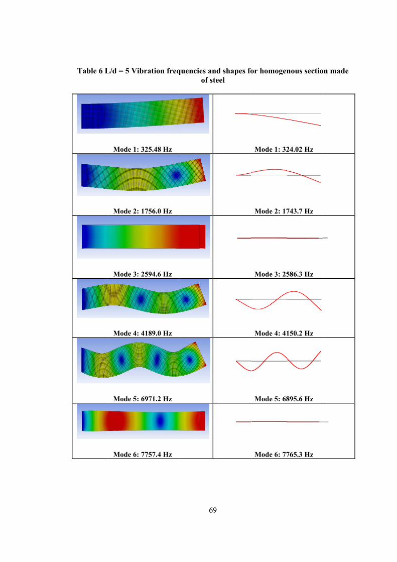
Table 6 L

L/d = 5 Vib

Mode 1: 3

Mode 2: 1

Mode 3: 2

Mode 4: 4

Mode 5: 6

Mode 6: 7

ration freq

325.48 Hz

1756.0 Hz

2594.6 Hz

4189.0 Hz

6971.2 Hz

7757.4 Hz

69

quencies anof st

9

nd shapes foteel

or homogen

Mode 1: 32

Mode 2: 17

Mode 3: 25

Mode 4: 41

Mode 5: 68

Mode 6: 77

nous sectio

24.02 Hz

743.7 Hz

586.3 Hz

150.2 Hz

895.6 Hz

765.3 Hz

on made

Mode 7

Mode 8:

Mode 9:

7: 9931.9 Hz

: 12818.0 Hz

: 12902.0 Hz

Table 6 (

z

z

70

(continued)

Mode 7:

Mode 8:

Mode 9:

: 9822.0 Hz

12774.9 Hz

12962.9 Hz

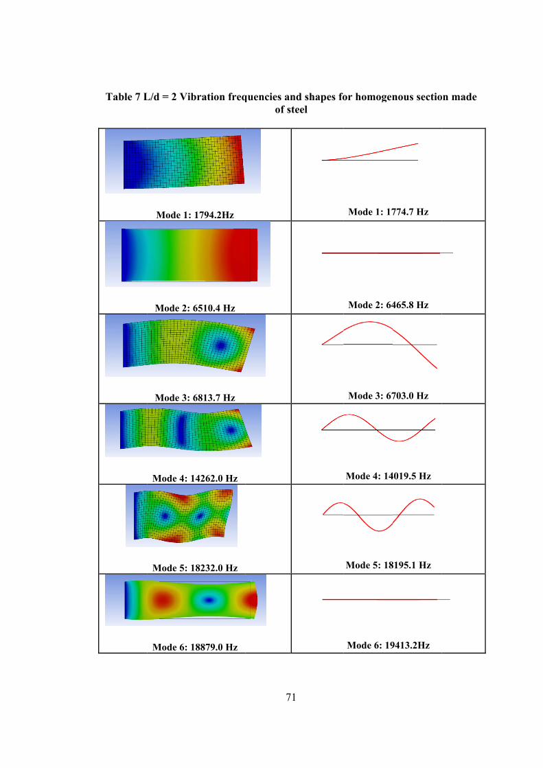
Table 7 L

L/d = 2 Vib

Mode 1: 1

Mode 2: 6

Mode 3: 6

Mode 4: 14

Mode 5: 18

Mode 6: 18

ration freq

1794.2Hz

6510.4 Hz

6813.7 Hz

4262.0 Hz

8232.0 Hz

8879.0 Hz

71

quencies anof st

1

nd shapes foteel

or homogen

Mode 1: 17

Mode 2: 64

Mode 3: 67

Mode 4: 14

Mode 5: 18

Mode 6: 19

nous sectio

774.7 Hz

465.8 Hz

703.0 Hz

4019.5 Hz

8195.1 Hz

9413.2Hz

on made

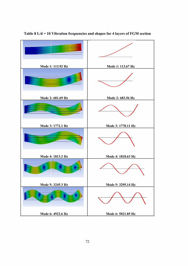
Table

8 L/d = 10

Mode 1

Mode 2

Mode 3

Mode 4

Mode 5

Mode 6

Vibration

1: 113.92 Hz

2: 681.69 Hz

3: 1772.1 Hz

4: 1813.2 Hz

5: 3245.3 Hz

6: 4922.6 Hz

frequencie

72

es and shappes for 4 lay

Mode 1:

Mode 2:

Mode 3:

Mode 4:

Mode 5:

Mode 6:

yers of FGM

113.67 Hz

683.56 Hz

1778.11 Hz

1818.63 Hz

3295.14 Hz

5021.85 Hz

M section

Mode 7: 5

Mode 8: 6

Mode 9: 8

Mode 10: 8

Mode 11:

Mode 12:

5377.7 Hz

6776.3 Hz

8697.5 Hz

8893.8 Hz

10724 Hz

12231 Hz

73

Table 8 (co

3

ontinued)

M

M

M

Mode 7: 53

Mode 8: 69

Mode 9: 90

Mode 10: 89

Mode 11: 11

Mode 12: 12

390.9 Hz

65.39 Hz

43.38 Hz

918.44 Hz

1183.3 Hz

2449.4 Hz

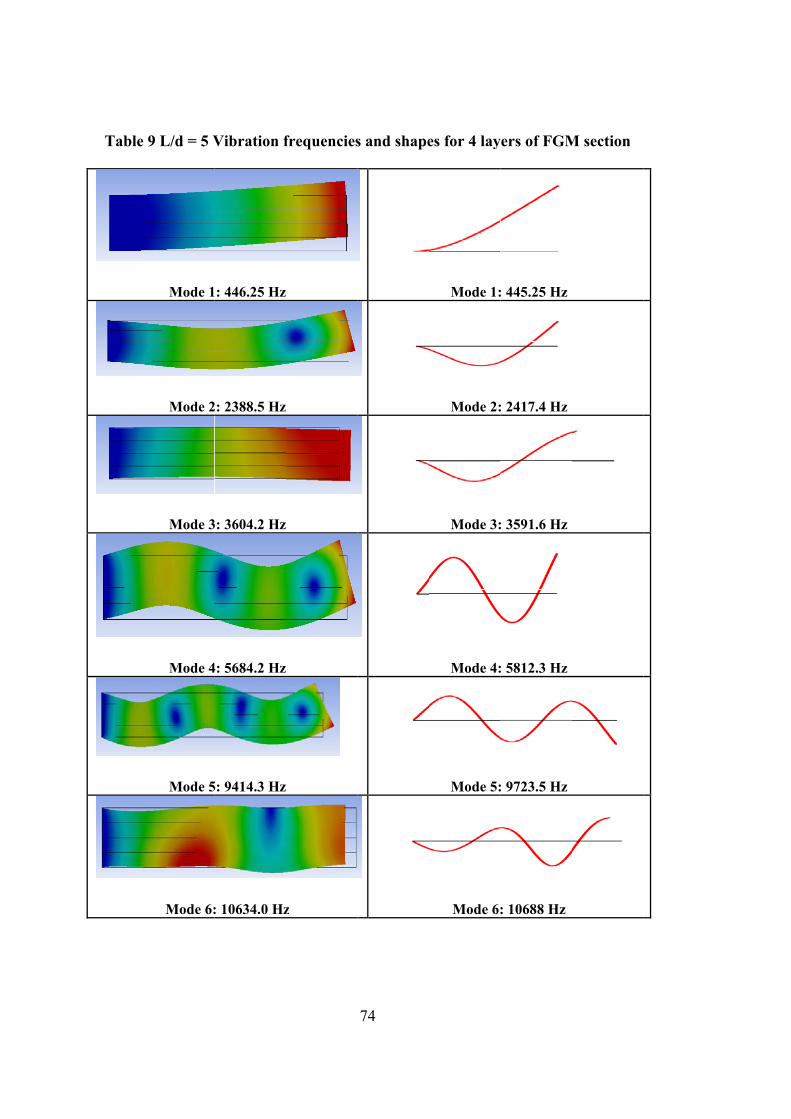
Table

e 9 L/d = 5 V

Mode 1

Mode 2

Mode 3

Mode 4

Mode 5

Mode 6:

Vibration f

1: 446.25 Hz

2: 2388.5 Hz

3: 3604.2 Hz

4: 5684.2 Hz

5: 9414.3 Hz

: 10634.0 Hz

frequencies

z

74

s and shape

es for 4 lay

Mode 1:

Mode 2:

Mode 3:

Mode 4:

Mode 5:

Mode 6:

yers of FGM

: 445.25 Hz

: 2417.4 Hz

: 3591.6 Hz

: 5812.3 Hz

: 9723.5 Hz

: 10688 Hz

M section

Mode 7: 1

Mode 8: 1

Mode 9: 1

Mode 10:

Mode 11:

Mode 12:

13410 Hz

16868 Hz

17603 Hz

20871 Hz

22380 Hz

23074 Hz

75

Table 9 (co

5

ontinued)

Mode 7: 13

Mode 8: 17

Mode 9: 1

Mode 10: 2

Mode 11: 2

Mode 12: 2

3979 Hz

7364.1 Hz

8542 Hz

22392 Hz

24320 Hz

25340 Hz

Table

10 L/d = 2

Mode 1

Mode 2

Mode 3

Mode 4

Mode 5

Mode 6

Vibration

1: 2450.1 Hz

2: 8527.3 Hz

3: 9753.4 Hz

4: 18969 Hz

5: 23908 Hz

6: 25022 Hz

frequencie

76

es and shappes for 4 lay

Mode 1:

Mode 2:

Mode 3:

Mode 4:

Mode 5:

Mode 6:

yers of FGM

2463.04 Hz

: 8523.3 Hz

10036.0 Hz

19785.8 Hz

: 25676 Hz

: 27398 Hz

M section

77

Table 11 Frequency comparison of proposed beam element and ANSYS model for rectangular steel section d=100 mm and b=100 mm

Beam Element SCF=5/6

Beam Element SCF=1

ANSYS Model Natural

Error SCF=5/6

Error SCF=1

1 82.89 82.97 83.072 0.23% 0.13%2 496.6 499.8 498.17 0.31% 0.33%3 1293.2 1293.2 1295.3 0.16% 0.16%4 1306.1 1323.3 1311.6 0.42% 0.89%5 2369.8 2418.8 2382.2 0.52% 1.54%6 3610.9 3710.4 3631.4 0.56% 2.18%7 3882.6 3882.7 3882.7 0.00% 0.00%8 4971.0 5138.1 4997.6 0.53% 2.81%9 6413.7 6481.5 6440.2 0.41% 0.64%10 6481.5 6662.9 6459.9 0.33% 3.14%11 7916.1 8259.4 7931.7 0.20% 4.13%12 9095.9 9095.9 9018 0.86% 0.86%1 324.02 325.25 325.48 0.45% 0.07%2 1743.7 1778.7 1756 0.70% 1.30%3 2586.3 2586.4 2594.6 0.32% 0.32%4 4150.2 4286.0 4189 0.93% 2.32%5 6895.6 7191.2 6971.2 1.08% 3.16%6 7765.3 7765.3 7757.4 0.10% 0.10%7 9822.0 10314.3 9931.9 1.11% 3.85%8 12774.9 12963.0 12818 0.34% 1.13%9 12962.9 13503.0 12902 0.47% 4.66%1 1774.7 1807.1 1794.2 1.09% 0.72%2 6465.8 6465.9 6510.4 0.69% 0.68%3 6703.0 7036.0 6813.7 1.62% 3.26%4 14019.5 14817.5 14262 1.70% 3.90%5 18195.1 19413.3 18232 0.20% 6.48%6 19413.2 19594.8 18879 2.83% 3.79%

2

ModeL/d

10

5

Steel Section

78

Table 12 Frequency comparison of proposed beam element and ANSYS model for FGM section d=100 mm and b=100 mm

Beam Element SCF=1 Natural

Frequencies (Hz)

ANSYS Model Natural Frequencies

(Hz)Error

1 113.67 113.92 0.22%2 683.56 681.69 0.27%3 1778.11 1772.1 0.34%4 1818.63 1813.2 0.30%5 3295.14 3245.3 1.54%6 5021.85 4922.6 2.02%7 5390.9 5377.7 0.25%8 6965.39 6776.3 2.79%9 9043.38 8697.5 3.98%10 8918.44 8893.8 0.28%11 11183.3 10724 4.28%

12 12449.4 12231 1.79%

1 445.25 446.25 0.22%2 2417.4 2388.5 1.21%3 3591.6 3604.2 0.35%4 5812.3 5684.2 2.25%5 9723.5 9414.3 3.28%6 10688 10634 0.51%7 13979 13410 4.24%8 17364.1 16868 2.94%9 18542 17603 5.33%10 22392 20871 7.29%11 24320 22380 8.67%

12 25340 23074 9.82%

1 2463.04 2450.1 0.53%2 8523.3 8527.3 0.05%3 10036 9753.4 2.90%4 19785.8 18969 4.31%5 25676 23908 7.40%

6 27398 25022 9.50%

L/d Mode

Top Alumina - Bottom Ceramics FGM Section

10

5

2

79

The modal analyses results for steel section are presented in Table 11.

As the length/depth ratio decreases, shear deformations turn out to be more

deterministic on the results of analyses. The proposed beam element is constituted in

accordance with Timoshenko’s beam theory. Since the plane sections remain plane

after deformation the beam is not capable of mocking the realistic shear

deformations. This lack of behavior for the beam element ends up with a statement

that as the length/depth ratio decreases the natural frequency error increases. On the

other hand for the axial modes the beam element gives less than 1% error even for

L/d=2.

Speaking of the FGM section, the same statements can be put forward for the error

values given in Table 12. In addition, the bending - axial coupling terms, aroused in

the evolution of FGM finite element formulation, end up with complicated mode

shapes. Such behavior of FGM makes it difficult to match between the modes of

ANSYS and the proposed beam element especially for fewer values of L/d.

80

81

CHAPTER 6

CONCLUSIONS

6.1. SUMMARY

The main purpose of this thesis is to represent a new force-based beam finite element

to be used in the analysis of functionally graded materials. For this purpose, force-

based formulation has been adapted to be compatible with a typical FGM section,

where the material properties vary through depth of the section. The proposed force-

based beam element has been compared with a previously developed displacement-

based beam finite element for regarding the non-linear behavior. Also vibration

analysis of the proposed beam element is verified with ANSYS results using 3D

solid elements.

6.2. CONCLUSIONS

The elastic behavior of the force-based element and the displacement beam

element yields the same results.

For the inelastic analyses of beams with FGM, 1 force-based element per half

span yields an error less than 1% whereas the error of 1 displacement-based

element per half span is about 40%.

For the vibration analyses, as length/depth ratio increases the errors for

frequencies of the proposed beam element tends to decrease.

The proposed beam element is able to determine even the axial-bending

mixed mode shapes and frequencies for L/d=10 and L/d=5.

82

It is getting more insistent to match the complex mode shapes as length/depth

ratio decreases.

6.3. RECOMMENDATIONS FOR FUTURE STUDY

For the yield behavior of alumina material in FGM model, Drucker–Prager yield

criteria can be utilized. By this means the proposed beam’s mechanical behavior can

be more realistic.

Thermo-mechanical analyses should be realized in order to investigate the

distribution of the temperature field under specified heat and/or body loadings.

In addition, a parametric study for functionally graded materials can be held out by

means of finite element analysis, to be utilized in the design process of FGM beams.

83

REFERENCES

Bocciarelli, M., G. Bolzon and G. Maier (2008). "A constitutive model of metal–ceramic functionally graded material behavior: Formulation and parameter identification." Computational Materials Science 43(1): 16-26.

Chakraborty, A., S. Gopalakrishnan and J. N. Reddy (2003). "A new beam finite element for the analysis of functionally graded materials." International Journal of Mechanical Sciences 45(3): 519-539.

Filippou, F. C. and G. L. Fenves (2004). Methods of Analysis for Earthquake-Resistant Structures. Earthquake Engineering, From Engineering Seismology to Performance-Based Engineering. Y. Bozorgnia and V. V. Bertero, CRC Press LLC.

Friedman, Z. and J. B. Kosmatka (1993). "An improved two-node timoshenko beam finite element." Computers & Structures 47(3): 473-481.

Hemmatnezhad, M., R. Ansari and G. H. Rahimi (2013). "Large-amplitude free vibrations of functionally graded beams by means of a finite element formulation." Applied Mathematical Modelling 37(18–19): 8495-8504.

Jha, D. K., T. Kant and R. K. Singh (2013). "A critical review of recent research on functionally graded plates." Composite Structures 96(0): 833-849.

Kieback, B., A. Neubrand and H. Riedel (2003). "Processing techniques for functionally graded materials." Materials Science and Engineering: A 362(1–2): 81-106.

Mohanty, S. C., R. R. Dash and T. Rout (2011). "Parametric instability of a functionally graded Timoshenko beam on Winkler's elastic foundation." Nuclear Engineering and Design 241(8): 2698-2715.

Molins, C., P. Roca and A. H. Barbat (1998). "Flexibility-based linear dynamic analysis of complex structures with curved-3D members." Earthquake Engineering & Structural Dynamics 27(7): 731-747.

84

Nakamura, T., T. Wang and S. Sampath (2000). "Determination of properties of graded materials by inverse analysis and instrumented indentation." Acta Materialia 48(17): 4293-4306.

Reddy, J. N. (1997). "On locking-free shear deformable beam finite elements." Computer Methods in Applied Mechanics and Engineering 149(1–4): 113-132.

Reddy, J. N. (2000). "Analysis of functionally graded plates." International Journal for Numerical Methods in Engineering 47(1-3): 663-684.

Reddy, J. N. and C. D. Chin (1998). "Thermomechanical analysis of functionally graded cylinders and plates." Journal of Thermal Stresses 21(6): 593-626.

Saritas, A. (2006). Mixed Formulation Frame Element for Shear Critical Steel and Reinforced Concrete Members. Ph.D. Dissertation, University of California , Berkeley.

Saritas, A. and O. Soydas (2012). "Variational base and solution strategies for non-linear force-based beam finite elements." International Journal of Non-Linear Mechanics 47(3): 54-64.

Soydas, O. (2013). A three dimensional mixed formulation nonlinear frame finite element based on Hu-Washizu functional. Ph.D., METU.

Soydas, O. and A. Saritas (2013). "An accurate nonlinear 3d Timoshenko beam element based on Hu-Washizu functional." International Journal of Mechanical Sciences 74(0): 1-14.

Spacone, E., V. Ciampi and F. C. Filippou (1996). "Mixed formulation of nonlinear beam finite element." Computers & Structures 58(1): 71-83.

85

APPENDIX A

DEFINITION OF VARIATION

Total energy functional is indicated in (3.4) and (3.5). The formulation will be

derived according to minimization of energy functional.

2 2

0

1[( ) ( )( )]

2

L

x x xy xy

A

P S T y U W dAdx (A.1)

The variation of a functional ( , , )F u w with respect to u is

0

( , , ) ( , , )lim

F u v w F u wu

(A.2)

where v is the test function that satisfies essential boundary conditions of the

corresponding differential equation.

Using (3.1),(3.2) and (3.3)

2 2

2 20

( )( , , ) ( )( , )1( , , )

2 ( )(( ) ( ) )

Lx x x

A

E y u y G y wP u w dAdx

y u y w

(A.3)

taking the derivative of (A.3) with respect to u

2 2 2 2

0

0

1( )(( ), , ) ( )( , ) ( )((( ) ) ( ) ) ( , , )

2

1[ ( ) (2 , , 2 , , ) ( ) (2 2 )]

2

1[ ( )(2 , , 2 , , ) ( )(2 2 )]

2

L

x x x

A

L

x x x x

A

x x x x

A

E y u v y G y w y u v y w dAdx P u w

u

E y u v y v y uv y v dAdx

u

u E y u v y v y uv y v dAdx

0

L

(A.4)

86

Applying integration by parts for the terms 00 0

, , , ,|L LL

x x x xxu v dx u v u vdx and

00 0, , , ,|

L LL

x x x xxv dx v vdx , (A.4) will transform into

0

0

[ ( )( , , ) ( )( )]

[ ( )[ ( )( ( ), ( ), ) ( )( ( ) ( ))] ]|

L

xx xx

A

L

x x

A

u v E y u y y u y dAdx

v x E y u x y x y u x y x dA

(A.5)

The terms in the last row of (A.5) are either representing the external forces or zero

depending on the boundary condition type of the freedom (EBC or NBC)

If the boundary condition type is essential, the term mentioned above will be zero

since the test functions have to satisfy the essential boundary conditions of the

corresponding differential equation ( ( ) 0EBCv x ). Otherwise the term clearly

represents the external forces since the shape functions are constituted in such a way

that they yield ( ) 1NBCv x at natural boundary conditions according to finite element

shape functions.

After handling the mentioned term above; substituting the terms defined in (3.7) into

(A.5) yields

0 1 11 11: , ,xx xxu I u I A u B (A.6)

The same procedure (taking derivative of ( , , )P u w with respect to w and ) can be

applied to acquire the other terms of (3.9).