Embed Size (px)
Citation preview

(DRAFT)
Finite Element Methods for Flow in PorousMedia
Juho Könnö
June 10, 2011
Abstract
This thesis studies the application of finite element methods to porous flow prob-
lems. Particular attention is paid to locally mass conserving methods, which are
very well suited for typical multiphase flow applications in porous media. The
focus is on the Brinkman model, which is a parameter dependent extension of
the classical Darcy model for porous flow taking the viscous phenomena into ac-
count. The thesis introduces a mass conserving finite element method for the
Brinkman flow, with complete mathematical analysis of the method. In addi-
tion, stochastic material parameters are considered for the Brinkman flow, and
parameter dependent Robin boundary conditions for the underlying Darcy flow.
All of the theoretical results in the thesis are also verified with extensive numer-
ical testing. Furthermore, many implementational aspects are discussed in the
thesis, and computational viability of the methods introduced, both in terms of
usefulness and computational complexity, is taken into account.
Tiivistelmä
Väitöskirja käsittelee elementtimenetelmän soveltamista houkoisen aineen vir-
taustehtäviin. Erityishuomion kohteena ovat lokaalisti massan säilyttävät ele-
menttimenetelmät, joiden tärkeys korostuu erityisesti käytännön sovelluksissa
tyypillisissä monifaasivirtauksissa. Huomion keskipisteenä on Brinkmanin mal-
li, joka laajentaa huokoiselle virtaukselle usein käytettyä Darcyn mallia otta-
malla huomioon myös viskoottiset efektit. Mallille esitellään massan säilyttä-
vä elementtimenetelmä, sekä menetelmän kattava matemaattinen analyysi. Li-
säksi väitöskirjassa tutkitaan stokastisten materiaaliparametrien mallintamis-
ta Brinkmanin tehtävän yhteydessä, sekä parametririippuvan Robin-tyyppisen
reunaehdon asettamista Darcyn tehtävälle. Kaikki teoreettiset tulokset on vah-
vistettu kattavin numeerisin kokein. Väitöskirjassa kiinnitetään myös huomiota
menetelmien käytännön toteutukseen ja laskennalliseen raskauteen, sekä nii-
den soveltuvuuteen käytännön ongelmiin.
2

Preface
This thesis was written at the Department of Mathematics and Systems
Analysis at Aalto University during the period 2008 – 2011.
Writing this thesis would not have been possible without the finan-
cial support from the Finnish Cultural Foundation, the Finnish Gradu-
ate School in Engineering Mechanics, Finnish Foundation for Technology
Promotion, and the Emil Aaltonen Foundation. In addition I would like
to recognize the financial support from the Finnish Research Programme
on Nuclear Waste Management (KYT2010) project.
Espoo, June 10, 2011,
Juho Könnö
3

Contents
Preface 3
Contents 5
List of Publications 7
Author’s Contribution 9
1 Introduction 11
2 Mathematical models for porous flow 15
2.1 The Darcy model . . . . . . . . . . . . . . . . . . . . . . . . . 17
2.2 The Brinkman model . . . . . . . . . . . . . . . . . . . . . . . 17
2.3 Local mass conservation - why? . . . . . . . . . . . . . . . . . 18
2.4 Stochastic permeability fields . . . . . . . . . . . . . . . . . . 20
3 Numerical methods 21
3.1 Discretizations of the H(div) space . . . . . . . . . . . . . . . 21
3.2 Enforcing continuity via penalization . . . . . . . . . . . . . . 22
3.3 Postprocessing for the pressure . . . . . . . . . . . . . . . . . 23
3.4 A posteriori estimators . . . . . . . . . . . . . . . . . . . . . . 25
3.5 Hybridization techniques . . . . . . . . . . . . . . . . . . . . . 25
3.6 The multi-level Monte Carlo method . . . . . . . . . . . . . . 27
4 Concluding remarks 29
Bibliography 31
Publications 33
5


List of Publications
This thesis consists of an overview and of the following publications which
are referred to in the text by their Roman numerals.
I Juho Könnö, Dominik Schötzau and Rolf Stenberg. Mixed Finite Ele-
ment Methods for Problems with Robin Boundary Conditions. SIAM
Journal on Numerical Analysis, 49(11), pp. 285-308, 2011.
II Juho Könnö and Rolf Stenberg. Analysis of H(div)-conforming Fi-
nite Elements for the Brinkman Problem. Accepted for publication in
Mathematical Models and Methods in Applies Sciences, doi:10.1142/
S0218202511005726, 2011.
III Juho Könnö and Rolf Stenberg. Numerical Computations with H(div)-
Finite Elements for the Brinkman Problem. Submitted to Computa-
tional Geosciences, Preprint: arXiv:1103.5338v1 2011.
IV Claude Gittelson, Juho Könnö, Christoph Schwab and Rolf Stenberg.
The Multi-Level Monte Carlo Finite Element Method for the Stochastic
Brinkman Problem. Submitted to Numerische Mathematik, Preprint:
ETH Zürich, Seminar für Angewandte Mathematik, Research Report
2011-31, 2011.
7


Author’s Contribution
Publication I: “Mixed Finite Element Methods for Problems withRobin Boundary Conditions”
Major parts of the analysis and writing, as well as all of the numerical
experiments, are due to the author.
Publication II: “Analysis of H(div)-conforming Finite Elements forthe Brinkman Problem”
The author is responsible for the writing and a major part of the analysis.
Publication III: “Numerical Computations with H(div)-FiniteElements for the Brinkman Problem”
The author is responsible for the writing and all of the numerical exam-
ples in the paper. The hybridization technique in Section 4 and the exten-
sion to non-constant permeability are due to the author.
Publication IV: “The Multi-Level Monte Carlo Finite Element Methodfor the Stochastic Brinkman Problem”
The author is responsible for writing Sections 5 and 7, as well as for adapt-
ing the finite element techniques and the analysis thereof to the stochas-
tic framework. All of the numerical computations are performed by the
author.
9

1. Introduction
In recent years a growing demand for efficient, accurate and reliable sim-
ulation methods has emerged in the field of geomechanics. In particular,
the modelling of fluid flow in porous media is a central problem within the
field with various applications in hydrogeology, soil contamination mod-
elling, and petroleum engineering, to name a few. Most subsurface flows
take place in different rock and soil types with varying porosities, thus
rendering problems in geomechanics very challenging numerically due to
highly irregular physical data, uncertainty in both the geometry and the
parameter values, and last but not least the sheer size of the problems
at hand. Another problematic aspect are the extremely long time scales,
with the longest simulated intervals ranging typically from tens of years
in petroleum engineering to extreme time intervals of tens of thousands
of years in nuclear waste disposal applications.
Applications in hydrogeology encompass e.g. groundwater modelling,
soil drainage, tracking the distribution of pollutants, and recently also
nuclear waste disposal. The growing need for advanced simulations is
to a great extent due to constantly tightening environmental regulations
of industrial installations requiring careful risk assessment. For exam-
ple, in undergound nuclear waste disposal it is of great importance to
accurately model the water breakthough time to the capsules containing
the radioactive waste with a timescale of tens of years, as well as the
transport of different chemical agents in the groundwater undermining
the structural integrity of the bentonite buffer during a period of thou-
sands of years. Naturally, in such a volatile application the reliability of
the computational results is a key issue.
Another important major application of subsurface flow models is petr-
oleum engineering. Although the first signs of the use of petroleum date
back to 4000 BC, it is only recently that the high demand for oil has in-
11

Introduction
duced a massive need for efficient extraction techniques, and thus for ad-
vanced simulation methods for enhanced oil recovery. The computational
models in petroleum engineering are characterized by very heteregenous
and possibly stochastic material data and the massive physical size of
the problems. Consequently, many of the numerical methods in subsur-
face flow modelling stem from the need to utilize the scarce computational
resources with utmost efficiency in massive reservoir simulations whilst
still retaining some essential properties such as local mass conservation
in the numerical methods employed.
Apart from geomechanical engineering, porous flow problems emerge in
a variety of industrial applications, ranging from e.g. filtration technology
and composite resin infusion to biomedical modelling of permeable cell
walls. For example, in resin infusion molding of composite laminates one
models the fiberglass or carbon fiber matrix as a porous medium. This
results in a two-phase flow problem with air and resin flowing both inside
the porous fibres as well as the void space left between the fibres.
This thesis addresses two porous flow models – namely the Darcy model
and the more complicated Brinkman model [19, 1, 2, 3]. In the following
we shall first introduce both of the models, and discuss the applicability of
the two to different physical problems. The thesis focuses on three distinct
problems related to the aforementioned flow models.
First, a parameter dependent boundary condition for the Darcy flow
model is analyzed. This Robin type boundary condition allows one to
move continuously between a pressure and a normal velocity boundary
condition. A similar boundary condition was analyzed in [20], but the ro-
bustness with respect to the parameter ε was not studied. Both a priori
and residual based a posteriori estimates robust in the parameter ε are
presented for the problem. It is also shown, that by using hybridization
for the velocity field, the resulting system matrix is not ill-conditioned in
the normal velocity boundary condition limit.
Next, a locally mass conserving finite element discretization of the Brink-
man flow model is analyzed. The approach taken in the thesis employs
H(div)-conforming finite elements to acertain the local conservation of
mass discussed later in detail in Chapters 2 and 3. The tangential conti-
nuity of the velocity field required by the Brinkman model is then weakly
enforced using a symmetric interior penalty Galerkin method. Similar
techniques have been analyzed for the Stokes flow in [11, 15, 23, 22],
whereas an approach based onH1-conforming finite elements for the Brink-
12

Introduction
man problem has been widely analyzed e.g. in references [14, 4, 12]. A
complete a priori and a residual based a posteriori analysis is presented,
and all of the results are verified by extensive numerical testing.
The third and final focal point of the thesis is the simulation of stochas-
tic material parameters for the Brinkman flow. In the rapidly growing
field of stochastic finite element methods, problems in soil mechanics play
an important role, since oftentimes the data for the permeability field
is naturally of stochastic nature. Here, the multi level Monte Carlo tech-
nique [5, 13] is applied to the Brikman problem with a log normal stochas-
tic permeability field. A stabilized conforming Stokes-based finite element
approach presented in [14] is adapted to meet the demands of the multi
level Monte Carlo method, and extensive numerical tests verify the re-
sults.
13

2. Mathematical models for porous flow
The quantities of interest in porous flow models are the pore pressure p
and the velocity u of the fluid. In the following we present phenomenolog-
ically the Darcy and Brinkman models, for a detailed and rigorous deriva-
tion, cf. [19, 1, 2] and the references therein.
Let µ denote the dynamic viscosity of the fluid. Roughly speaking, vis-
cosity describes the thickness of the fluid. For example, water is often
described as a thin and honey as a thick fluid. In engineering applica-
tions the viscosities of the co-flowing fluids ofter vary by several orders of
magnitude. In resin infusion the epoxy resin is very thick with a viscosity
of several hundreds of centipoise (cP) compared to the air present in the
matrix. Similarly, water is often used as the driving fluid in enhanced
oil recovery, which is very thin with a viscosity of approximately one cen-
tipoise when compared to heavy crude oils having viscosities of hundreds
or even thousands of centipoise.
The permeability is denoted by K. In general, permeability is a sym-
metric tensor quantity. In numerous practical situations in geomechanics
the permeability tensor is of the diagonal form. However, when using e.g.
upscaling methods [18] for the permeability field, the resulting effective
permeability tensor is often highly anisotropic. The unit for permeability
is Darcy, 1 D = 9.869233× 10⁻¹³ m2, commonly permeabilities are given in
mD. Typically the permeability is a highly heterogeneous quantity, and
the magnitude of variations might be extremely large. In Table 2.1 some
typical permeabilities for different types of soil and rock are presented [7].
To clarify the heterogeneity of the permeability field, the logarithm of
the permeability field for one layer of the the SPE10 benchmark dataset [10]
describing a typical highly heterogenous oil reservoir is plotted in Fig-
ure 2.1. Evidently, the jumps in the material parameters in realistic
reservoir applications are often of several orders of magnitude. Further-
15

Mathematical models for porous flow
Permeability mD Property Examples
108 – 106 Pervious Clean gravel
106 – 104 Pervious Clean sand, gravel and sand
104 – 101 Semipervious Oil rocks, peat, fine sand
101 – 10−1 Semipervious Sandstone, stratified clay
10−1 – 10−3 Impervious Limestone, dolomite, clay
10−3 – 10−5 Impervious Granite, breccia
Table 2.1. Permeabilities for different soil and rock types.
more, Figure 2.1 also shows how the permeability fields in certain types
of reservoirs are very chanellized localizing the flow to certain regions
of the computational domain and thus underlining the need for adaptive
methods in the numerical simulation of subsurface flows. Similarly, in
nuclear waste disposal one is interested in the flow of groundwater in the
extremely narrow void channels between the bentonite blocks.
In addition, it should be kept in mind that the derived quantities of in-
terest, such as the well pressures and the production rates in petroleum
engineering, as well as the saturation distribution depend both on the
pore pressure p and the fluid velocity u. Similarly, in industrial appli-
cations one wishes to keep the hydraulic pressures on a safe level while
simulatenously e.g. maximizing the flow through an oil filter. Thus it is
essential to design finite elements methods that perform equally well for
both of the aforementioned variables.
Figure 2.1. Logarithm of the permeability field in layer 68 of the SPE10 dataset in mD.
16
Mathematical models for porous flow
2.1 The Darcy model
The Darcy flow model is the simplest and by far the most widely used
porous flow model. In the Darcy model the flow is directly proportional to
the pressure gradient via the relation [19, 7]
u = − 1µ
K∇p. (2.1)
Assuming the fluid to be incompressible, the Darcy equations read
µK−1u +∇p = f , (2.2)
div u = g. (2.3)
Here, the loading f comprises of body loadings to the fluid, most com-
monly gravity effects. The function g is a source term, describing e.g.
injection and production wells in a groundwater or oil reservoir.
Normally one enforces either the pressure or the normal velocity on the
boundary. In a nuclear waste management application, for example, one
might prescribe the groundwater pressure on the boundary between the
bentonite buffer and the borehole wall in the bedrock, and a no-flow con-
dition on the boundary between the bentonite and the waste capsule. In
article I we analyse the following Robin type boundary condition for the
Darcy problem,
εu·n + p = εun,0 + p0. (2.4)
Here, ε ≥ 0 is a parameter which allows one to move between the limiting
pressure boundary condition p = p0 as ε = 0 and the normal flow boundary
condition u·n = un,0 as ε→∞.
2.2 The Brinkman model
In the Brinkman model, one adds an effective viscosity term to the Darcy
model. Thus the model constitutes a parameter dependent combination of
the porous Darcy flow and the viscous Stokes flow. The Brinkman model is
best suited for modelling very porous materials and domains with cracks
or flow channels. The main advantage of the Brinkman model is the abil-
ity to move from the Darcy regime to the Stokes regime and back by alter-
ing the material parameters only. With µ denoting the effective viscosity of
the fluid, the Brinkman equations for an incompressible fluid read [19, 18]
17
Mathematical models for porous flow
−µ∆u + µK−1u +∇p = f , (2.5)
div u = g. (2.6)
A common choice for µ is to take the effective viscosity equal to the dy-
namic viscosity, i.e. µ = µ, however more refined models depending on
e.g. the porosity φ of the porous medium exist, see e.g. [18].
Mathematically the nature of the problem changes radically depending
on the ratio of the coefficients of the two velocity terms in equation (2.5).
For very large permeabilities the flow takes place in almost void space,
and the viscous part dominates. In this situation the flow is essentially
of the Stokes type, whereas for more impermeable materials the Darcy
part is the dominant term. Therefore the numerical method for solving
the Brinkman equation must be chosen carefully to assure stability and
accuracy of the method for all possible parameter values. For example
in reservoir simulation a large portion of the domain is typically in the
Darcy regime, but on the other hand in e.g. filter applications the void
space governed by the Stokes limit constitutes a major part of the domain.
This motivates the design of numerical methods that perform well in both
regimes and simultaneously allow for a seamless transition between the
two limiting models.
An approach based on finite elements originally designed for the Darcy
problem is covered in this thesis in articles II and III. Advantages of
the chosen approach include the intrisic local mass conservation property
of the finite element space and the ability to enhance the pressure ap-
proximation afterwards by a postprocessing scheme presented in paper
II. However, these elements are more complex to implement and com-
putationally more demanding than discretizations based on Stokes-type
elements analyzed in e.g. [14, 4].
2.3 Local mass conservation - why?
A central part of the thesis deals with finding a locally mass conserving
finite element method for the Brikman problem. But what makes this
property so important and desirable? To shed light on the issue, let us
recall that in practice almost all applications of porous flow models are
multiphase problems. That is, two or more fluids such as oil and water
18
Mathematical models for porous flow
or air and epoxy resin co-exist in the porous matrix. For simplicity, let us
demonstrate the importance of the local mass conservation property in the
simplest possible framework by considering a two phase incompressible
Darcy flow of oil and water with no capillary or gravity effects.
Let u = uo + uw be the total flow, in which uo and uw are the velocities
for the oil and water components, respectively. Since the flow is assumed
incompressible, we have
div u = 0 (2.7)
in the absence of sources or sinks. The water saturation S describes the
fraction of water of the total pore volume inside the porous matrix. The
saturation evolves in time as [9]
∂S
∂t+ div(fw(S)u) = gw, (2.8)
in which fw(S) is the saturation dependent flow fraction of water and gw
the source loading for the water component. Using the product rule for
divergence yields
∂S
∂t+ f ′w(S)∇S·u + fw(S)div u = gw. (2.9)
Clearly, the last term on the left hand side should vanish for an incom-
pressible flow. However, it is insufficient for the divergence to vanish
globally in the weak sense, since this could lead to spurious modes that
create artificial sources or sinks in individual elements. Thus we try to
find a method that satisfies the equilibrium property
div Vh ⊂ Qh, (2.10)
and the commutative diagram property
div Rh = Phdiv. (2.11)
Here the finite dimensional spaces Vh andQh are the approximation spaces
for the velocity and pressure, respectively. Rh is a special interpolation
operator for H(div,Ω) functions to Vh, and Ph is the L2-projection to Qh.
For details on the properties of the interpolation operator Rh, cf. arti-
cle II and the references therein. These properties quarantee that the
aforementioned spurious modes cannot occur. Since the time intervals
simulated in geomechanics are typically very long, from days to years, it
is of utmost importance that accumulation of unphysical saturation does
not occur during the computations.
19

Mathematical models for porous flow
2.4 Stochastic permeability fields
As mentioned, in soil mechanics one often encounters permeabily fields for
which only some statistical quantities are known. The aim is to simulate
such flow fields based on data such as the covariance and mean value of
the permeability field numerically. One of the most common models for
the permeability field is the log normal model. That is, the logarithm of
the permeability field is normally distributed. Thus the permeability field
is of the form
K = K0 exp (G), (2.12)
in which G is an Rd-valued, symmetric Gaussian field and K0 is a sym-
metric, positive definite d×dmatrix. The random field G has the Karhunen-
Loève expansion
G =∞∑
n=1
Yn
√λnΦn, (2.13)
in which (λn,Φn) are the eigenpairs of the covariance operator corre-
sponding to the random field G, and Yn are standard normal random
variables. For details, see e.g. [5] and article IV. In simple cases, the
eigenpairs for the covariance operator can be computed explicitly in some
simple domains, such as in a square or a circle. However, in a more gen-
eral setting one has to solve the eigenpairs numerically using e.g. finite
elements.
For computations, the infinite Karhunen-Loève series (2.13) must be
truncated. Thus the permeability field K is approximated with a trun-
cated field KN as
KN := K0 exp
(N∑
n=1
Yn
√λnΦn
). (2.14)
In article IV a multi level Monte Carlo method is considered for such a
permeability field. In a multi level Monte Carlo method the key ingredient
is to compute the samples on multiple nested meshes balancing the error
between the discretization error and the stochastic truncation error. The
analysis can be easily adapted to other models with log normal random
fields, too.
20
3. Numerical methods
In this section the main numerical methods deployed in the articles are
covered. The details of applying these techniques to each of the individual
problems in the thesis are presented in the articles, thus the main focus
here is to shed light on the ideas behind each of the different numerical
techniques and the underlying reasons for using a specific method.
3.1 Discretizations of the H(div) space
The space H(div,Ω) is composed of those functions u for which it holds
u ∈ L2(Ω) and div u ∈ L2(Ω). For the discretized space Vh the condition
Vh ⊂ H(div,Ω) translates into a continuity condition over the interele-
ment boundaries E ∈ Eh of the mesh Kh. More exactly, one requires that
the normal component u·n is continuous across the interelement bound-
aries.
Typically H(div)-conforming finite element spaces appear in the context
of mixed methods, for example we seek for the velocity of the fluid in Vh
and the pressure in Qh. In what follows, the spaces Vh and Qh are chosen
such that the method is stable, and that the equilibrium property
divVh ⊂ Qh (3.1)
and the commutative diagram property (2.11) hold. Consequently, the
weak divergence condition
(div u, q) = (g, q), ∀q ∈ Qh (3.2)
yields div u = Phg, in which Ph : L2(Ω) → Qh is the L2-projection to the
pressure space. Thus one immediately recognizes that for example the
incompressibility condition
div u = 0 (3.3)
21

Numerical methods
is satisfied exactly forH(div,Ω)-conforming elements satisfying (3.1). This
is the main motivation for such an approach to the Brinkman problem in
papers II and III. Oftentimes this property is referred to as local mass
conservation. As an example we consider in the following the simple first
order Brezzi-Douglas-Marini (BDM) element [8] for which
Vh = v ∈ H(div,Ω) | v|K ∈ [P1(K)]2, (3.4)
and the corresponding pressure space is
Qh = q ∈ L2(Ω) | q|K ∈ P0(K). (3.5)
The degrees of freedom for this element are the average and the first mo-
ment over the element edges, cf. Figure 3.1. The pressure space is discon-
tinuous over the interelement edges.
Figure 3.1. Degrees of freedom for the lowest-order BDM element
3.2 Enforcing continuity via penalization
It is often beneficial to relax the continuity requirements to some extent,
however in return some extra work has to be done in order to stabilize the
method. As mentioned earlier, only the normal component of the velocity
is required to be continuous in the case of H(div)-conforming elements. In
order to approximate the second order term describing the viscous effects
in the Brinkman model, the continuity of the tangential component is
weakly enforced akin to traditional discontinuous Galerkin (DG) methods.
This matter is discussed in detail in article II.
To fix ideas, consider the scalar Poisson problem
−∆u = f, in Ω, (3.6)
u = 0, on ∂Ω
22

Numerical methods
discretized with elementwise discontinuous finite elements from the space
Vh = v ∈ L2(Ω) | v|K ∈ Pk(K). Due to the discontinuity multiplication
by an arbitrary test function v ∈ Vh and partial integration of the first
equation yields ∑K∈Kh
(∇u,∇v)K − 〈 ∂u∂n
, v〉∂K = (f, v). (3.7)
To stabilize the method, we modify the weak formulation as follows:
(∇u,∇v) +∑
E∈Eh
(α
hE〈[[u]], [[v]]〉E − 〈 ∂u
∂n, [[v]]〉E − 〈[[u]], ∂v
∂n〉E)
= (f, v).
(3.8)
Here [[· ]] and · denote the jump and average on the edge E, respectively.
The above symmetric interior penalty Galerkin (SIPG) formulation (see
e.g. [21]) guarantees that for a suitably chosen stabilization parameter α
the formulation is stable and an optimal convergence rate with respect to
the polynomial degree of the space Vh is attained. In the context of setting
Dirichlet boundary conditions the above formulation is often referred to
as Nitsche’s method [17].
In articles II and III the SIPG formulation is employed to stabilize cer-
tain families of H(div)-conforming elements for the Brinkman problem,
as well as to enforce the boundary conditions weakly. The resulting fi-
nite element approximation is thus intrinsically locally mass conserving
and stable for all parameter values of the Brinkman model. In addition,
weakly enforcing the boundary conditions alleviates the numerical prob-
lems related to handling boundary layers stemming from no-flow bound-
ary conditions when approaching the Darcy limit.
3.3 Postprocessing for the pressure
As a model problem, the Darcy problem with the material parameters set
to unity is considered. In the discretized form we seek a velocity-pressure
pair (uh, ph) ∈ Vh ×Qh ⊂ H(div,Ω)× L2(Ω) such that
(u,v)− (div v, p) = (f ,v), ∀v ∈ Vh, (3.9)
−(div u, q) = −(g, q), ∀q ∈ Qh,
in which f and g are given sufficiently smooth loading functions.
To analyze the convergence of the finite element discretization, the fol-
23

Numerical methods
lowing mesh dependent norm is used for the pressure
‖p‖2h =∑
K∈Kh
‖∇p‖20,K +∑
E∈Eh
1hE‖[[p]]‖20,E , (3.10)
whilst for the velocity the L2-norm is employed. Note, that due to the
equilibrium property (3.1) we need not separetely estimate the error in
the divergence, since div uh = Phg. This yields the following suboptimal
convergence result for the pressure
‖Php− ph‖h ≤ Ch (3.11)
when the lowest order Brezzi-Douglas-Marini elements are employed. The
fact that the pressure solution ph only converges to the L2-projection Php
of the exact solution onto the finite element space Qh is simply due to the
lack of approximation properties of the pressure space, which in this case
is that of elementwise constant functions. However, a simple postprocess-
ing procedure can be shown to remedy this by seeking the postprocessed
pressure p∗h in an augmented space [16]. For example, for the first order
BDM element we choose
Q∗h = q ∈ L2(Ω) | q|K ∈ P2(K) (3.12)
and compute the postprocessed pressure p∗h ∈ Q∗h through
Php∗h = ph, (3.13)
(∇p∗h,∇q)K = (uh,∇q)K ∀q ∈ (I − Ph)Q∗h|K . (3.14)
It can then be shown [16], that full convergence rate is recovered for the
pressure, that is
‖p− ph‖h ≤ Ch. (3.15)
Note, that the postprocessed pressure is still discontinuous across the in-
terelement boundaries.
The postprocessing method can be applied to a wide variety of differ-
ent families of H(div)-conforming elements. In articles I, II and III this
technique is applied to more complicated problems to recover the optimal
convergence rate for the pressure variable. It is noteworthy that the pro-
cedure is performed elementwise thus being computationally inexpensive
compared to solving the original linear system, and also allowing for effi-
cient parallelization due to the localized nature.
24
Numerical methods
3.4 A posteriori estimators
In the analysis of finite element methods the error estimates are divided
into two categories - namely a priori and a posteriori estimates. The for-
mer are asymptotic error estimates of the form
‖u− uh‖1 ≤ Ch, (3.16)
which for example for the Poisson problem (3.6) tells that the error in
the H1(Ω)-norm is directly dependent on the mesh size h. However, the
constant C depends on some higher Sobolev norm of the exact solution u,
and thus cannot be computed in practice since the exact solution u is not
known.
On the other hand, in a posteriori estimates one seeks for an estimator η
which is a function of the discrete solution uh and the loading and bound-
ary condition functions. The aim is to find an estimator satisfying e.g. for
the model Poisson problem
cη ≤ ‖u− uh‖1 ≤ Cη. (3.17)
For this simple problem, such an estimator is
η2 =∑
K∈Kh
h2K‖∆uh + f‖20,K +
∑E∈Eh
hE‖[[∂uh
∂n]]‖20,E , (3.18)
in which [[· ]] denotes the jump of a function and n is the normal vector on
a face E ∈ Eh.
The constants c and C should not depend on the solution or the com-
putational mesh. However, sometimes these constants are unknown and
might depend e.g. on the shape of the domain, but they are nevertheless
known to be bounded. For parameter dependent problems, such as the
Robin-type boundary conditions in I and the Brinkman problem in II and
III, it is crucial that the constants are also independent of the parame-
ters. Deriving such parameter independent a posteriori bounds is one of
the key ingredients in this thesis.
3.5 Hybridization techniques
Sometimes it is desirable to break the continuity of the finite element
space on all or a certain subset of the interelement boundaries, and en-
force the continuity on these edges via Lagrange multipliers. Such tech-
niques are known as hybridized methods.
25
Numerical methods
The model mixed finite element problem (3.9) can be hybridized on all
internal edges as follows [6, 8]: Find (uh, ph,mh) ∈ Vh×Qh×Mh such that
(uh,v)−∑
K∈Kh
(div v, ph)K +∑
K∈Kh
〈v·n∂K ,mh〉∂K = (f ,v), (3.19)
−∑
K∈Kh
(div uh, q)K = (g, q), (3.20)
∑K∈Kh
〈uh·n∂K , r〉∂K = 0 (3.21)
for all (v, q, r) ∈ Vh × Qh ×Mh, in which Vh corresponds to the space Vh
with no continuity restrictions across interelement boundaries and n∂K
is the outer normal of the element K. Mh is a suitably chosen space of
Lagrange multipliers on the hybridized edges, e.g. for the lowest-order
BDM elements Mh is composed of first-order polynomials on the edges
E ∈ Eh.
The algebraic system corresponding to the hybridized equations is of the
form
Au + Bp+ Cm = f
BT u = g
CT u = 0,
in which A is a block diagonal matrix and (u, p,m) are now the coefficient
vectors associated with the finite element solution. One can now eliminate
the velocity and pressure variables ending up with a system for the La-
grange multipliers only. For example for the lowest order BDM elements
the blocksize of the matrix A is only 6×6, thus inverting A is computation-
ally very cheap. The resulting system matrix for the Lagrange multipliers
is of the form
CT (A−1B(BT A−1B)−1BT A−1 −A−1)C. (3.22)
This matrix is symmetric and positive definite [8] in contrast to the origi-
nal saddle point system, and hence well-suited for standard linear solvers.
Hybridization can also be easily adapted to domain decomposition by hy-
bridizing the finite element spaces only on the skeleton of the domain de-
composition mesh, and using subdomain solvers for inverting the matrix
A simultaneously on several computational nodes. Hybridization tech-
niques are considered in detail for both the Darcy problem and the Brink-
man problem in articles I and III, respectively.
26
Numerical methods
3.6 The multi-level Monte Carlo method
As previously mentioned, the permeability K is often known only as a
statistical quantity. That is, one has a stochastic model or uncertain mea-
surement data for the expected value and covariance of the permeabil-
ity field, thus underlining the importance of finding efficient simulation
methods for stochastic porous flow models. Traditional Monte Carlo meth-
ods rely on randomizing several realizations of the stochastic field and
computing a corresponding finite element solution for the quantities of
interest, which are then averaged to get quantities such as the expected
value of the velocity and pressure fields. A major drawback of traditional
Monte Carlo methods is that they are computationally very expensive.
As a remedy, multi level Monte Carlo methods have been proposed and
analyzed in e.g. [5, 13]. They are based on a hierarchy of finite element
discretizations and a varying level of approximation for the stochastic
parameter. The number of Monte Carlo samples per mesh level is var-
ied based on the convergence properties of the Karhunen-Loève expan-
sion (2.13) of the stochastic parameter. In paper IV the multi level Monte
Carlo method is applied to the Brinkman equations with a stochastic per-
meability field, and combined with a robust stabilized mixed finite ele-
ment method based on [14].
From the finite element point of view, a major challenge is to find a sta-
ble finite element method, such that the finite element spaces are nested
on a hierarchy of uniformly refined meshes to keep the workload low in
the multi level method. In addition, for stabilized methods, the depen-
dence of the stabilization parameter on the stochastic quantities must be
carefully studied. Due to the high number of samples computed and the
fact that virtually no internode communication is required, the method is
very well suited for massively parallel computations.
27


4. Concluding remarks
The main findings in this thesis can be summarized as follows.
I In this article the Darcy problem with a parameter dependent boundary
condition is studied. We introduce a weak formulation for enforcing the
boundary condition, along with a rigorous a priori and a posteriori anal-
ysis. The postprocessing method of [16] for the scalar variable is shown
to be applicable for this type of a problem, thus yielding optimal conver-
gence rates for the proposed method. It is shown that all the estimates
are independent of the parameter ε in the boundary condition, and all
of the theoretical results are verified with numerical tests.
II The article presents a complete and rigorous analysis of applyingH(div)-
conforming finite elements for the Brinkman problem. A suitable mesh
dependent norm for the problem is presented, in which we prove opti-
mal convergence estimates robust in the effective viscosity parameter t.
Thus the proposed method is applicable for the whole range of problems
from the Darcy flow to a viscous Stokes flow covered by the Brinkman
model. We also extend the aforementioned postprocessing method to the
Brinkman equations to achieve optimal convergence rate for the pres-
sure. The residual based a posteriori indicator introduced is shown to
be both reliable and efficient for all values of the parameter t ≥ 0.
III This paper is a continuation of paper II. The estimates are extended to
cover a non-constant permeability field, and a hybridization technique is
presented for the SIPG formulation of the problem. We also address ap-
plying the hybridization method to domain decomposition. A major part
of the paper deals with numerically verifying both the results in paper
II, as well as the new results presented in this paper. In addition, the
29

Concluding remarks
applicability of the a posteriori indicator to adaptive mesh refinement is
demonstrated employing realistic material data.
IV In this work the stochastic Brinkman problem with a log normal per-
meability field is studied. Rigorous error estimates are derived both
for the stochastic and the spatial discretization errors. A Stokes-based
stabilized finite element method proposed in [14] is modified to fulfill
the requirements of the multi level Monte Carlo method. In particular,
great attention is given to analyzing the computational complexity of
the method. Finally, all of the results are verified with extensive numer-
ical tests, verifying both the predicted convergence behaviour, as well as
the work load estimates.
30
Bibliography
[1] G. Allaire. Homogenization of the Navier-Stokes equations in open setsperforated with tiny holes. I. Abstract framework, a volume distribution ofholes. Arch. Rational Mech. Anal., 113(3):209–259, 1990.
[2] G. Allaire. Homogenization of the Navier-Stokes equations in open setsperforated with tiny holes. II. Noncritical sizes of the holes for a volumedistribution and a surface distribution of holes. Arch. Rational Mech. Anal.,113(3):261–298, 1990.
[3] T. Arbogast and H. L. Lehr. Homogenization of a Darcy-Stokes systemmodeling vuggy porous media. Comput. Geosci., 10(3):291–302, 2006.
[4] S. Badia and R. Codina. Unified stabilized finite element formulations forthe Stokes and the Darcy problems. SIAM J. Numer. Anal., 47(3):1971–2000, 2009.
[5] A. Barth, C. Schwab, and N. Zollinger. Multi-Level Monte-Carlo FiniteElement Method for Elliptic PDEs with Stochastic Coefficients. TechnicalReport 2010-10(to appear in Numerische Mathematik), Seminar for AppliedMathematics (SAM), ETH Zurich, 2010.
[6] M. Baudoiun Fraejis de Veubeke. Displacement and equilibrium models inthe finite element method. In Stress analysis, (O.C Zienkiewics and G.S,pages 145–197. Wiley, 1965.
[7] J. Bear. Dynamics of Fluids in Porous Media. American Elsevier, 1972.
[8] F. Brezzi and M. Fortin. Mixed and hybrid finite element methods, vol-ume 15 of Springer Series in Computational Mathematics. Springer-Verlag,New York, 1991.
[9] Z. Chen, G. Huan, and Y. Ma. Computational Methods for Multiphase Flowsin Porous Media (Computational Science and Engineering 2). Society forIndustrial and Applied Mathematics, Philadelphia, PA, USA, 2006.
[10] M. A. Christie and M. J. Blunt. Tenth SPE comparative solution project: Acomparison of upscaling techniques. SPE Reservoir Eval. Eng., 4(4):308–317, 2001.
[11] B. Cockburn, G. Kanschat, and D. Schötzau. A note on discontinuousGalerkin divergence-free solutions of the Navier-Stokes equations. J. Sci.Comput., 31(1-2):61–73, 2007.
31

Concluding remarks
[12] C. D’Angelo and P. Zunino. A finite element method based on weightedinterior penalties for heterogeneous incompressible flows. SIAM Journalon Numerical Analysis, 47(5):3990–4020, 2009.
[13] M. B. Giles. Multilevel Monte Carlo path simulation. Oper. Res., 56(3):607–617, 2008.
[14] M. Juntunen and R. Stenberg. Analysis of finite element methods for theBrinkman problem. Calcolo, 47(3):129–147, 2010.
[15] G. Kanschat and D. Schötzau. Energy norm a posteriori error estimationfor divergence-free discontinuous Galerkin approximations of the Navier-Stokes equations. Internat. J. Numer. Methods Fluids, 57(9):1093–1113,2008.
[16] C. Lovadina and R. Stenberg. Energy norm a posteriori error estimates formixed finite element methods. Math. Comp., 75:1659–1674, 2006.
[17] J. Nitsche. Über ein Variationsprinzip zur Lösung von Dirichlet-Problemenbei Verwendung von Teilräumen, die keinen Randbedingungen unterwor-fen sind. Abh. Math. Sem. Univ. Hamburg, 36:9–15, 1971. Collection ofarticles dedicated to Lothar Collatz on his sixtieth birthday.
[18] P. Popov, Y. Efendiev, and G. Qin. Multiscale modeling and simulations offlows in naturally fractured Karst reservoirs. Commun. Comput. Phys.,6(1):162–184, 2009.
[19] K. R. Rajagopal. On a hierarchy of approximate models for flows of incom-pressible fluids through porous solids. Math. Models Methods Appl. Sci.,17(2):215–252, 2007.
[20] J. Roberts and J.-M. Thomas. Mixed and hybrid finite element methods. InP. Ciarlet and J. Lions, editors, Handbook of Numerical Analysis, volume II:Finite Element Methods (Part 1), pages 523–639. North-Holland, 1991.
[21] T. Rusten, P. S. Vassilevski, and R. Winther. Interior penalty precondi-tioners for mixed finite element approximations of elliptic problems. Math.Comp., 65(214):447–466, 1996.
[22] J. Wang, Y. Wang, and X. Ye. A robust numerical method for Stokes equa-tions based on divergence-free H(div) finite element methods. SIAM J. Sci.Comput., 31(4):2784–2802, 2009.
[23] J. Wang and X. Ye. New finite element methods in computational fluiddynamics by H(div) elements. SIAM J. Numer. Anal., 45:1269–1286, May2007.
32

Publication I
Juho Könnö, Dominik Schötzau and Rolf Stenberg. Mixed Finite ElementMethods for Problems with Robin Boundary Conditions. SIAM Journal onNumerical Analysis, 49(11), pp. 285-308, 2011.
c© 2011 Society for Industrial and Applied Mathematics.Reprinted with permission.
33


Copyright © by SIAM. Unauthorized reproduction of this article is prohibited.
SIAM J. NUMER. ANAL. c© 2011 Society for Industrial and Applied MathematicsVol. 49, No. 1, pp. 285–308
MIXED FINITE ELEMENT METHODS FOR PROBLEMS WITHROBIN BOUNDARY CONDITIONS∗
JUHO KONNO†, DOMINIK SCHOTZAU‡ , AND ROLF STENBERG†
Abstract. We derive new a priori and a posteriori error estimates for mixed finite element dis-cretizations of second-order elliptic problems with general Robin boundary conditions, parameterizedby ε ≥ 0. The estimates are robust in ε, ranging from pure Dirichlet conditions to pure Neumannconditions. We also show that hybridization leads to a well-conditioned linear system. A series ofnumerical experiments is presented that verify our theoretical results.
Key words. mixed finite element methods, Robin boundary conditions, parameterized bound-ary conditions, a posteriori estimates, postprocessing
AMS subject classifications. 65N30, 65N15
DOI. 10.1137/09077970X
1. Introduction. We consider the dual mixed finite element method for second-order elliptic equations subject to general Robin boundary conditions. We parame-terize these by ε ≥ 0, with natural Dirichlet conditions corresponding to ε = 0 andNeumann conditions to the limit ε → ∞. For the mixed method the Neumann con-ditions are essential conditions and could be explicitly enforced. However, we preferto see the method implemented in the same way for all possible boundary conditionsand then the Neumann conditions are obtained by penalization, i.e., by choosing εsufficiently large.
Let us recall that the situation for a primal (displacement) finite element methodis the opposite, namely Neumann conditions are natural and Dirichlet conditionsessential, and the latter are penalized by choosing ε “small.” For this case it is wellknown that the problem is ill-conditioned in two ways. The error estimates are notindependent of ε and the stiffness matrix becomes ill-conditioned as ε → 0. We remarkhere that in [8] Nitsche’s method was extended to general Robin boundary conditionsyielding a primal finite element formulation avoiding this ill-conditioning.
Is the mixed method, too, ill-conditioned near the Neumann limit ε → ∞? Inthis paper we will show that this is not the case. We will prove both a priori anda posteriori error estimates that are uniformly valid, independently of the value ofthe parameter ε. We also show that by using hybridization the stiffness matrix iswell-conditioned. To the best of our knowledge, these results have not been reportedearlier in the literature. Robin conditions are treated in [12], but the robustness withrespect to the parameter ε was not studied.
The outline of this paper is as follows. In the next section, we recall the mixedfinite element method for problems with Robin boundary conditions. In section 3,we derive a priori error estimates and prove an optimal L2-bound for the error in the
∗Received by the editors December 11, 2009; accepted for publication (in revised form) November10, 2010; published electronically February 15, 2011.
http://www.siam.org/journals/sinum/49-1/77970.html†Department of Mathematics and Systems Analysis, Aalto University, P.O. Box 11100, FIN-
00076 AALTO, Espoo, Finland ([email protected], [email protected]). The first author’s workwas supported by the Finnish Cultural Foundation.
‡Mathematics Department, University of British Columbia, Vancouver, BC V6T 1Z2, Canada([email protected]). This author’s work was supported in part by the Natural Sciences andEngineering Research Council of Canada (NSERC).
285

Copyright © by SIAM. Unauthorized reproduction of this article is prohibited.
286 JUHO KONNO, DOMINIK SCHOTZAU, AND ROLF STENBERG
flux. In section 4, we analyze the postprocessing method of [14, 15], which enhancesthe accuracy of the displacement variable. In section 5, we introduce a residual-baseda posteriori error estimator and establish its reliability and efficiency. In section 6,we consider the solution of the problem by hybridization and show that this approachleads to a well-conditioned linear system. A set of numerical examples that verify theε-robustness of our estimates is presented in section 7. Finally, we end the paper withsome concluding remarks in section 8.
Throughout this paper, we use standard notation. We denote by C, C1, C2, etc.,generic positive constants that are not necessarily identical at different places, but arealways independent of ε and the mesh size.
2. Mixed finite element methods. In this section, we introduce two familiesof mixed finite element methods for the mixed form of Poisson’s equation with Robinboundary conditions.
2.1. Model problem. We consider the following model problem:
σ −∇u = 0 in Ω,(2.1)div σ + f = 0 in Ω,(2.2)
subject to the general Robin boundary conditions
(2.3) εσ·n = u0 − u + εg on ∂Ω.
Here, Ω ⊂ Rn, n = 2, 3, is a bounded polygonal or polyhedral Lipschitz domain,f ∈ L2(Ω) is a given load, and u0 ∈ L2(∂Ω) and g ∈ L2(∂Ω) are prescribed data onthe boundary of Ω. With these assumptions, we have (σ, u) ∈ H(div, Ω) × L2(Ω).The vector n denotes the unit outward normal vector on ∂Ω. The boundary condi-tions (2.3) are parameterized by the nonnegative function ε ≥ 0. For simplicity, weassume ε to be piecewise constant on the boundary (with respect to the partitionof ∂Ω induced by a triangulation of Ω). In the limiting case ε = 0, we obtain theDirichlet boundary conditions
(2.4) u = u0 on ∂Ω.
On the other hand, if ε → ∞ everywhere on ∂Ω, we recover the Neumann boundaryconditions
(2.5) σ·n = g on ∂Ω.
Assuming the solution and boundary data are sufficiently smooth, we first notethat (σ, u) satisfies
(σ, τ ) + (div τ , u) − 〈u, τ ·n〉∂Ω = 0 ∀τ ∈ H(div, Ω),(2.6)
(div σ, v) + (f, v) = 0 ∀v ∈ L2(Ω).(2.7)
Then we solve for u in the expression (2.3) for the boundary conditions and insert theresult into (2.6). We find that
aε(σ, τ ) + (div τ , u) = 〈u0 + εg, τ ·n〉∂Ω ∀τ ∈ H(div, Ω),(2.8)
(div σ, v) + (f, v) = 0 ∀v ∈ L2(Ω),(2.9)

Copyright © by SIAM. Unauthorized reproduction of this article is prohibited.
MIXED FE METHODS WITH ROBIN BOUNDARY CONDITIONS 287
with aε(σ, τ ) defined by
aε(σ, τ ) = (σ, τ ) + 〈εσ·n, τ ·n〉∂Ω.
Here, we denote by (·, ·) the standard L2-inner product over Ω, and by 〈·, ·〉∂Ω the oneover the boundary ∂Ω. By introducing the bilinear form
Bε(σ, u; τ , v) = aε(σ, τ ) + (div τ , u) + (div σ, v),
we thus obtain the following weak form of (2.1)–(2.2): Find (σ, u) such that
(2.10) Bε(σ, u; τ , v) + (f, v) = 〈u0 + εg, τ ·n〉∂Ω
for all (τ , v) ∈ H(div, Ω) × L2(Ω).
2.2. Mixed finite element discretization. In order to discretize the vari-ational problem (2.10), let Kh be a regular and shape-regular partition of Ω intosimplices. As usual, the diameter of an element K is denoted by hK , and the globalmesh size h is defined as h = maxK∈Kh
hK . We denote by E0h the set of all interior
faces of Kh, and by E∂h the set of all boundary faces. We write hE for the diameter of
a face E. Throughout this paper we shall refer to both edges in 2D and faces in 3Dgenerically as faces.
Mixed finite element discretization of (2.10) is based on finite element spacesSh × Vh ⊂ H(div, Ω) × L2(Ω) of piecewise polynomial functions with respect to Kh.We will focus here on the Raviart–Thomas (RT) and Brezzi–Douglas–Marini (BDM)families of elements [11, 10, 4, 3, 5]. That is, for an approximation of order k ≥ 1, theflux space Sh is taken as one of the following two spaces:
SRTh = σ ∈ H(div, Ω) |σ|K ∈ [Pk−1(K)]n ⊕ xPk−1(K), K ∈ Kh ,
SBDMh = σ ∈ H(div, Ω) |σ|K ∈ [Pk(K)]n, K ∈ Kh ,
(2.11)
where Pk(K) denotes the polynomials of total degree less than or equal to k on K,and Pk−1(K) is the homogeneous polynomials of degree k− 1. For both choices of Sh
above, the displacements are approximated in the multiplier space
(2.12) Vh = u ∈ L2(Ω) |u|K ∈ Pk−1(K), K ∈ Kh .The spaces are chosen such that the following equilibrium property holds:
(2.13) div Sh ⊂ Vh.
The mixed finite element method now consists of finding (σh, uh) ∈ Sh×Vh such that
(2.14) Bε(σh, uh; τ , v) + (f, v) = 〈u0 + εg, τ ·n〉∂Ω
for all (τ , v) ∈ Sh×Vh. We remark that, by the equilibrium condition (2.13), we haveimmediately the identity
(2.15) div σh = −Phf,
with Ph denoting the L2-projection onto Vh.
3. A priori error estimates. In this section, we derive a priori error estimatesfor the method in (2.14). The main result of this section is an ε-robust and optimalL2-bound for the error in the fluxes.
Copyright © by SIAM. Unauthorized reproduction of this article is prohibited.
288 JUHO KONNO, DOMINIK SCHOTZAU, AND ROLF STENBERG
3.1. Stability. We begin by introducing the jump of a piecewise smooth scalarfunction u. To that end, let E = ∂K∩∂K ′ be an interior face shared by two elementsK and K ′. Then the jump of f over E is defined by
(3.1) [[f ]] = f |K − f |K′ .
Next, we recall the following well-known trace estimate: for a face E of an elementK, there holds
(3.2) hE‖σ‖20,E ≤ C‖σ‖2
0,K ∀σ ∈ Sh.
Stability will be measured in mesh-dependent norms. For the fluxes, we define
(3.3) ||σ||2ε,h = ‖σ‖20 +
∑E∈E∂
h
(ε + hE)‖σ·n‖20,E .
Here, we denote by ‖ · ‖0,D the L2-norm over a set D. In the case where D = Ω, wesimply write ‖ · ‖0. For the displacement variables, we introduce the norm
(3.4) |||u|||2ε,h =∑
K∈Kh
‖∇u‖20,K +
∑E∈E0
h
1hE
‖[[u]]‖20,E +
∑E∈E∂
h
1ε + hE
‖u‖20,E.
The continuity of the bilinear forms in the above norms follows by straightforwardestimation.
Lemma 3.1. We have
|aε(σ, τ )| ≤ ||σ||ε,h||τ ||ε,h, σ, τ ∈ Sh,(3.5)
|(div σ, u)| ≤ C||σ||ε,h|||u|||ε,h, σ ∈ Sh, u ∈ Vh.(3.6)
Furthermore, it holds that
(3.7) |Bε(σ, u; τ , v)| ≤ C(||σ||ε,h + |||u|||ε,h
)(||τ ||ε,h + |||v|||ε,h
)for all σ, τ ∈ Sh and u, v ∈ Vh.
Proof. The bound (3.5) is a simple consequence of the Cauchy–Schwarz inequality:
aε(σ, τ ) = (σ, τ ) + 〈εσ·n, τ ·n〉∂Ω
= (σ, τ ) +∑
E∈E∂h
〈ε1/2σ·n, ε1/2τ ·n〉E ≤ ||σ||ε,h||τ ||ε,h.
To prove (3.6), we use partial integration, elementary manipulations, and the Cauchy–Schwarz inequality to obtain
(div σ, u) = −∑
K∈Kh
(σ,∇u)K +∑
K∈Kh
〈σ·n∂K , u〉∂K
≤∑
K∈Kh
‖σ‖0,K‖∇u‖0,K +∑
E∈E0h
h12E‖σ·n‖0,Eh
− 12
E ‖[[u]]‖0,E
+∑
E∈E∂h
(ε + hE)12 ‖σ·n‖0,E(ε + hE)−
12 ‖u‖0,E,
Copyright © by SIAM. Unauthorized reproduction of this article is prohibited.
MIXED FE METHODS WITH ROBIN BOUNDARY CONDITIONS 289
with n∂K denoting the unit outward normal on ∂K. The trace estimate (3.2) anda repeated application of the Cauchy–Schwarz inequality then readily prove (3.6).Finally, the continuity bound (3.7) follows directly from (3.5) and (3.6).
Next, we address the coercivity of the form aε.Lemma 3.2. There is a constant C > 0 such that
aε(σ, σ) ≥ C||σ||2ε,h ∀σ ∈ Sh.
Proof. Since aε(σ, σ) = ‖σ‖20+∑
E∈E∂h
ε‖σ·n‖20,E, the trace estimate (3.2) readily
yields the desired result.Finally, we prove the following inf-sup condition for the divergence form.Lemma 3.3. There exists a constant C > 0 such that
supσ∈Sh
(div σ, u)||σ||ε,h
≥ C|||u|||ε,h ∀u ∈ Vh.
Proof. The proof is an extension of that of [9, Lemma 2.1]. Since SRTh ⊂ SBDM
h ,we need only prove the condition in the Raviart–Thomas case. We recall that, on anelement K, the local degrees of freedom for the RT family are given by the moments
〈σ·n∂K , z〉E ∀z ∈ Pk−1(E), E ⊂ ∂K,
(σ, z)K ∀z ∈ [Pk−2(K)]n.
Now let u ∈ Vh be arbitrary. We then define σ ∈ SRTh by setting on each element K:
〈σ·n∂K , z〉E =1
hE〈[[u]], z〉E ∀z ∈ Pk−1(E), E ∈ E0
h, E ⊂ ∂K,
〈σ·n∂K , z〉E =1
ε + hE〈u, z〉E ∀z ∈ Pk−1(E), E ∈ E∂
h , E ⊂ ∂K,
(σ, z)K = −(∇u, z)K ∀z ∈ [Pk−2(K)]n.
Choosing z = [[u]] ∈ Pk−1(E) and z = ∇u ∈ [Pk−2(K)]n gives
〈σ·n∂K , [[u]]〉E =1
hE‖[[u]]‖2
0,E, E ∈ E0h, E ⊂ ∂K,
〈σ·n∂K , [[u]]〉E =1
ε + hE‖u‖2
0,E, E ∈ E∂h , E ⊂ ∂K,
(σ,∇u)K = −‖∇u‖20,K.
Then we employ partial integration over each element and apply the defining momentsfor σ:
(div σ, u) =∑
K∈Kh
−(σ,∇u)K +∑
K∈Kh
〈σ·n∂K , u〉∂K
=∑
K∈Kh
‖∇u‖20,K +
∑E∈E0
h
1hE
‖[[u]]‖20,E +
∑E∈E∂
h
1ε + hE
‖u‖20,E
= |||u|||2ε,h.
(3.8)
Copyright © by SIAM. Unauthorized reproduction of this article is prohibited.
290 JUHO KONNO, DOMINIK SCHOTZAU, AND ROLF STENBERG
Moreover, an explicit inspection of the degrees of freedom readily yields
(3.9) ||σ||ε,h ≤ C|||u|||ε,h.
Identity (3.8) and the bound (3.9) give the desired inf-sup condition.By combining continuity (Lemma 3.1), coercivity (Lemma 3.2), and the inf-sup
condition (Lemma 3.3), we readily obtain the following stability result.Lemma 3.4. There is a constant C > 0 such that
sup(τ ,v)∈Sh×Vh
Bε(σ, u; τ , v)||τ ||ε,h + |||v|||ε,h
≥ C(||σ||ε,h + |||u|||ε,h) ∀(σ, u) ∈ Sh × Vh.
3.2. Error estimates. We are now ready to derive a priori error estimates. Tothat end, let (σ, u) be the solution of (2.10), and let (σh, uh) be the mixed finiteelement approximation of (2.14).
Let Rh : [H1(Ω)]n → Sh be the RT or BDM interpolation operator [5]. It satisfies
(3.10) (div (σ − Rhσ), v) = 0 ∀v ∈ Vh,
as well as the commuting diagram property
(3.11) div Rhσ = Ph div σ;
see, e.g., [5]. Moreover, we note that the equilibrium property (2.13) implies
(3.12) (div τ , u − Phu) = 0 ∀τ ∈ Sh.
Remark 3.5. In order for Rhσ to be well-defined locally on an element K, someextra regularity is required for σ. More precisely, the boundary traces σ·n∂K are onlydefined in H−1/2(∂K), and thus the moments specifying Rhσ are not well-defined.It can be shown [5] that sufficient smoothness requirements are σ ∈ H(div, Ω) andσ|K ∈ [Ls(K)]d with an exponent s > 2.
Proposition 3.6. There is a constant C > 0 such that
||σh − Rhσ||ε,h + |||uh − Phu|||ε,h ≤ C‖σ − Rhσ‖0.
Proof. By the stability result in Lemma 3.4 there exists (τ , v) ∈ Sh × Vh suchthat ||τ ||ε,h + |||v|||ε,h ≤ C and
||σh − Rhσ||ε,h + |||uh − Phu|||ε,h ≤ Bε(σh − Rhσ, uh − Phu; τ , v).
Using the consistency of the mixed method and properties (3.10), (3.12), we obtain
Bε(σh − Rhσ, uh − Phu; τ , v)= aε(σh − Rhσ, τ ) + (div τ , uh − Phu) + (div (σh − Rhσ), v)= aε(σ − Rhσ, τ ) + (div τ , u − Phu) + (div (σ − Rhσ), v)
= (σ − Rhσ, τ ) +∑
E∈E∂h
ε〈(σ − Rhσ)·n, τ ·n〉E .
Then the defining moments for RT or BDM interpolation yield (noting that ε isfacewise constant)
(3.13)∑
E∈E∂h
ε〈(σ − Rhσ)·n, τ ·n〉E = 0,
Copyright © by SIAM. Unauthorized reproduction of this article is prohibited.
MIXED FE METHODS WITH ROBIN BOUNDARY CONDITIONS 291
so that
Bε(σh − Rhσ, uh − Phu; τ , v) = (σ − Rhσ, τ ).
Thus, we conclude that
||σh − Rhσ||ε,h + |||uh − Phu|||ε,h ≤ ‖σ − Rhσ‖0‖τ‖0 ≤ C‖σ − Rhσ‖0,
which completes the proof.In what follows, we denote by ‖ · ‖k the standard Sobolev norm of order k. The
following theorem is the main result of this section.Theorem 3.7. Assume that σ ∈ [Hk(Ω)]d for RT elements and σ ∈ [Hk+1(Ω)]d
for BDM elements. Then we have the approximation bound
(3.14) ||σh −Rhσ||ε,h + |||Phu− uh|||ε,h ≤
Chk‖σ‖k for RT elements,
Chk+1‖σ‖k+1 for BDM elements.
Moreover, we have the following optimal a priori error estimate for the L2-error inthe flux:
(3.15) ‖σ − σh‖0 ≤
Chk‖σ‖k for RT elements,
Chk+1‖σ‖k+1 for BDM elements.
Proof. The bound (3.14) is an immediate consequence of Proposition 3.6 andthe approximation properties of Rh; see, e.g., [5]. The error estimate (3.15) followsreadily from the triangle inequality, the consistency bound in Proposition 3.6, andthe approximation properties of Rh.
Remark 3.8. We point out that the quantity |||Phu−uh|||ε,h in (3.14) is supercon-vergent. As in [9], this fact allows us to enhance the displacement approximation vialocal postprocessing; see section 4 below. We further emphasize that the constant Cin the error bound (3.15) is independent of ε.
4. Postprocessing. In this section, we introduce a local postprocessing for thedisplacement and prove an optimal error estimate in the postprocessed displacement.
4.1. Postprocessing method. Let uh be the displacement obtained by themixed method (2.14). The postprocessed displacement u∗
h is sought in the augmentedspace V ∗
h ⊃ Vh defined as
(4.1) V ∗h =
u∗ ∈ L2(Ω) |u∗|K ∈ Pk(K), K ∈ Kh for RT elements,
u∗ ∈ L2(Ω) |u∗|K ∈ Pk+1(K), K ∈ Kh for BDM elements.
The postprocessed displacement u∗h is now defined on each element K by the condi-
tions
Phu∗h = uh,(4.2)
(∇u∗h,∇v)K = (σh,∇v)K ∀v ∈ (I − Ph)V ∗
h |K ;(4.3)
cf. [14, 15]. Here, we recall that Ph is the L2-projection onto Vh.In order to analyze the error in the postprocessed displacement u∗
h, we introducethe modified bilinear form
(4.4) B∗ε,h(σ, u∗; τ , v∗) = Bε(σ, u∗; τ , v∗) +
∑K∈Kh
(∇u∗ − σ,∇(I − Ph)v∗)K .
Copyright © by SIAM. Unauthorized reproduction of this article is prohibited.
292 JUHO KONNO, DOMINIK SCHOTZAU, AND ROLF STENBERG
Then we will consider the modified variational problem: Find (σh, u∗h) ∈ Sh × V ∗
h
such that
(4.5) B∗ε,h(σh, u∗
h; τ , v∗) + (Phf, v∗) = 〈u0 + εg, τ ·n〉∂Ω
for all (τ , v∗) ∈ Sh×V ∗h . The following proposition relates the solution of the modified
problem (4.5) to that of the original problem (2.14). Its proof is exactly the same asthe one for the standard mixed methods considered in [9, Lemma 2.4].
Proposition 4.1. Let (σh, u∗h) ∈ Sh × V ∗
h be the solution of problem (4.5) andset uh = Phu∗
h. Then (σh, uh) ∈ Sh×Vh is the solution of the original problem (2.14).Conversely, if (σh, uh) ∈ Sh × Vh is the solution of the original problem (2.14) andu∗
h is the postprocessed displacement obtained from uh, then (σh, u∗h) ∈ Sh ×V ∗
h is thesolution of problem (4.5).
In order to show the stability of the modified method (4.5), we shall first statethe following useful result whose proof is nearly identical to that of [9, Lemma 2.5].
Lemma 4.2. There exist constants C1 > 0, C2 > 0 such that for every u∗ ∈ V ∗h
there holds
(4.6) |||u∗|||ε,h ≤ |||Phu∗|||ε,h + |||(I − Ph)u∗|||ε,h ≤ C2|||u∗|||ε,h,
as well as
(4.7) C1|||u∗|||ε,h ≤ |||Phu∗|||ε,h +
( ∑K∈Kh
‖∇(I − Ph)u∗‖20,K
)1/2
≤ C2|||u∗|||ε,h.
Since (I − Ph)u∗ is L2-orthogonal to constant functions, there exists a third constantC3 > 0 such that
(4.8) |||(I − Ph)u∗|||ε,h ≤ C3
( ∑K∈Kh
‖∇(I − Ph)u∗‖20,K
)1/2
.
With exactly the same arguments as in [9, Lemma 2.6], we then have the followinginf-sup stability result for the modified bilinear form B∗
ε,h.Proposition 4.3. There exists a constant C > 0 such that
(4.9) sup(τ ,v∗)∈Sh×Q∗
h
B∗ε,h(σ, u∗; τ , v∗)||τ ||ε,h + |||v∗|||ε,h
≥ C(||σ||ε,h + |||u∗|||ε,h) ∀(σ, u∗) ∈ Sh × V ∗h .
4.2. Error in the postprocessed displacement. Now we state and prove apriori error estimates for the postprocessed displacement u∗
h. As before, let (σ, u) bethe solution of (2.10), and let (σh, u∗
h) be the postprocessed finite element approxi-mation of (4.5). We now have the following result.
Theorem 4.4. There holds
||σh − Rhσ||ε,h + |||u − u∗h|||ε,h ≤ C
(‖σ − Rhσ‖0 + inf
u∗∈V ∗h
|||u − u∗|||ε,h
).
Moreover, if we assume that (σ, u) ∈ [Hk(Ω)]d × Hk+1(Ω) for RT elements and(σ, u) ∈ [Hk+1(Ω)]d × Hk+2(Ω) for BDM elements, then we have the error estimate
‖σ − σh‖0 + |||u − u∗h|||ε,h ≤
Chk(‖σ‖k + ‖u‖k+1) for RT elements,
Chk+1(‖σ‖k+1 + ‖u‖k+2) for BDM elements.
Copyright © by SIAM. Unauthorized reproduction of this article is prohibited.
MIXED FE METHODS WITH ROBIN BOUNDARY CONDITIONS 293
Note that the constant Cis independent of ε and the rates of convergence are optimalwith respect to the polynomial degree of the approximation.
Proof. Let u∗ ∈ V ∗h . From Proposition 4.3 it follows that there is a tuple (τ , v∗) ∈
Sh × V ∗h such that ||τ ||ε,h + |||v∗|||ε,h ≤ C and
||σh − Rhσ||ε,h + |||u∗h − u∗|||ε,h ≤ B∗
ε,h(σh − Rhσ, u∗h − u∗; τ , v∗).
From the definition of the method (4.5), we then have
B∗ε,h(σh − Rhσ, u∗
h − u∗; τ , v∗)
= B∗ε,h(σ − Rhσ, u− u∗; τ , v∗) + (f − Phf, v∗)
= aε(σ − Rhσ, τ ) + (div τ , u − u∗) + (div (σ − Rhσh), v∗) + (f − Phf, v∗)
+∑
K∈Kh
(∇(u − u∗) − (σ − Rhσ),∇(I − Ph)v∗)K .
Due to the commuting diagram property (3.11) and (2.2), div σ = −f , there holds
(div (σ − Rhσ), v∗) = (div σ − Phdiv σ, v∗) = (−f + Phf, v∗),
so that
B∗ε,h(σh − Rhσ, u∗
h − u∗; τ , v∗) = aε(σ − Rhσ, τ ) + (div τ , u − u∗)
+∑
K∈Kh
(∇(u − u∗) − (σ − Rhσ),∇(I − Ph)v∗)K .
As in the proof of Proposition 3.6, we use (3.13) and get
aε(σ − Rhσ, τ ) = (σ − Rhσ, τ ) ≤ C‖σ − Rhσ‖0.
Moreover, by integration by parts as in the continuity proof of Lemma 3.1, we have
(div τ , u − u∗) ≤ C||τ ||ε,h|||u − u∗|||ε,h ≤ C|||u − u∗|||ε,h.
Furthermore, by Lemma 4.2 the last term can be bounded by∑K∈Kh
(∇(u − u∗) − (σ − Rhσ),∇(I − Ph)v∗)K
≤ C(‖σ − Rhσ‖0 + |||u − u∗|||ε,h)|||v∗|||ε,h
≤ C(‖σ − Rhσ‖0 + |||u − u∗|||ε,h).
Since v∗ ∈ V ∗h was arbitrary, the first assertion is proved.
The error estimate is now an immediate consequence of the bound for σh −Rhσand the triangle inequality. Then assuming sufficient regularity, the convergence resultfollows from the interpolation properties of Rh and approximation properties of thespace V ∗
h .
5. A posteriori estimates. We now derive a residual-based a posteriori estima-tor for the postprocessed solution (σh, u∗
h). We point out that using the postprocessedsolution is vital for obtaining an estimator whose local residual terms are properlymatched with respect to their convergence properties; see also [9].

Copyright © by SIAM. Unauthorized reproduction of this article is prohibited.
294 JUHO KONNO, DOMINIK SCHOTZAU, AND ROLF STENBERG
5.1. Error estimator. For an element K, we define the local error indicators
η21,K = ‖∇u∗
h − σh‖20,K , η2
2,K = h2K‖f − Phf‖2
0,K .
For an interior face E ∈ E0h, we introduce the jump indicator
η2E = h−1
E ‖[[u∗h]]‖2
0,E .
Let u0 be the L2-projection of u0 onto Pk(E) for RT and onto Pk+1(E) for BDMelements. Similarly, gh is the L2-projection of g onto Pk−1(E) for RT elements andonto Pk(E) for BDM elements. We define the boundary estimator as
(5.1) η2E =
1ε + hE
‖ε(σh · n − gh) + u∗h − u0‖2
0,E .
We emphasize that the boundary estimator (5.1) will be evaluated exactly as a poly-nomial of degree k or k + 1 for RT and BDM elements, respectively. For the approx-imation of the Dirichlet datum u0 we set
η2u0,E =
1ε + hE
‖u0 − u0‖20,E.
To also take into account the approximation of g, we introduce the set
(5.2) E∂h,+ =
E ∈ E∂
h | ε|E > 0
of all boundary faces E with a nonvanishing ε|E . For a boundary face E ∈ E∂h,+, we
then introduce the indicator related to the approximation of g by setting
η2g,E = hE‖g − gh‖2
0,E.
Summing up these local indicators, our error estimator is given by
(5.3) η =
⎛⎝ ∑K∈Kh
(η21,K + η2
2,K
)+∑
E∈E0h
η2E +
∑E∈E∂
h
(η2E + η2
u0,E) +∑
E∈E∂h,+
η2g,E
⎞⎠ 12
.
Here we also include the data approximation terms in the estimator η, even thoughthey are neglected in the numerical experiments shown in section 7.
Remark 5.1. Note that, for ε = 0, the indicator ηg,E can be omitted in thedefinition of η. The resulting estimator then coincides with the ones derived in thepapers [9, 13] for homogeneous and inhomogeneous Dirichlet boundary conditions,respectively.
5.2. Reliability. To derive an upper bound for the a posteriori estimator ηin (5.3), we denote by (σ, u) the solution of the perturbed problem where we replace gby gh:
(5.4) Bε(σ, u; τ , v) + (f, v) = 〈u0 + εgh, τ ·n〉∂Ω
for all (τ , v) ∈ H(div, Ω) × L2(Ω). Since
〈gh, τ ·n〉E = 〈g, τ ·n〉E ∀τ ∈ Sh, E ∈ E∂h ,

Copyright © by SIAM. Unauthorized reproduction of this article is prohibited.
MIXED FE METHODS WITH ROBIN BOUNDARY CONDITIONS 295
it is clear that the finite element approximations (σh, u∗h) are in fact also approxima-
tions to (σ, u).We will make use of the following saturation assumption [8, 9]: Let Kh/2 be a
uniformly refined subtriangulation of Kh, obtained by dividing each simplex K ∈ Kh
into 2n elements. We denote by σh/2 and u∗h/2 the flux and postprocessed displacement
obtained on the finer mesh Kh/2. The saturation assumption can now be formulatedas follows.
Assumption 5.2 (saturation assumption). There exists a constant β < 1 suchthat
‖σ − σh/2‖0 + |||u − u∗h/2|||ε,h/2 ≤ β (‖σ − σh‖0 + |||u − u∗
h|||ε,h) .
The following result establishes the reliability of the estimator η.Theorem 5.3. Suppose that Assumption 5.2 holds. Then there exists a con-
stant C > 0 such that
(5.5) ‖σ − σh‖0 + |||u − u∗h|||ε,h ≤ Cη.
Proof. We proceed in several steps.Step 1. Let (σ, u) and (σ, u) denote the solutions of (2.10) and (5.4), respectively.
The difference (σ − σ, u − u) in the displacement then satisfies the equations
(σ − σ, τ ) + (div τ , u − u) − 〈u − u, τ ·n〉∂Ω = 0 ∀τ ∈ H(div, Ω),(5.6)
(div (σ − σ), v) = 0 ∀v ∈ L2(Ω),(5.7)
with the following boundary condition on ∂Ω:
ε(σ − σ) + u− u = ε(g − gh).
Inserting (τ , v) = (σ − σ, u− u) as test functions yields
‖σ − σ‖20 −
∑E∈E∂
h,+
〈(σ − σ)·n, u − u〉E = 0.
Using the boundary condition, we conclude that
‖σ − σ‖20 +
∑E∈E∂
h,+
1ε‖u − u‖2
0,E =∑
E∈E∂h,+
〈g − gh, u − u〉E .
Let P0 be the L2-projection onto the piecewise constants. For any face E ∈ E∂h,+ with
E ⊂ ∂K, we now use the definition of gh and standard approximation results to get
〈g − gh, u − u〉E = 〈g − gh, u − u − P0(u − u)〉E ≤ Ch12E‖g − gh‖0,E‖∇(u − u)‖0,K .
We thus readily obtain
‖σ − σ‖20 +
∑E∈E∂
h,+
1ε‖u − u‖2
0,E ≤ C∑
E∈E∂h,+
η2g,E .
The definition of the norm ||| · |||ε,h, the inequality (ε|E +hE)−1 ≤ ε|−1E for all E ∈ E∂
h,+,and the fact that u − u|E = 0 on all faces with ε|E = 0 yield
(5.8) ‖σ − σ‖0 + |||u − u|||ε,h ≤ Cη.

Copyright © by SIAM. Unauthorized reproduction of this article is prohibited.
296 JUHO KONNO, DOMINIK SCHOTZAU, AND ROLF STENBERG
Step 2. From the triangle inequality and the bound (5.8), we obtain
‖σ − σh‖0 + |||u − u∗h|||ε,h ≤ Cη + ‖σ − σh‖0 + |||u − u∗
h|||ε,h.
It is thus sufficient to bound the error of the finite element approximation (σh, u∗h) to
the perturbed solution (σ, u) in (5.4). From Assumption 5.2, we conclude that
‖σ − σh‖0 + |||u − u∗h|||ε,h ≤ 1
1 − β
(‖σh/2 − σh‖0 + |||u∗
h/2 − u∗h|||ε,h/2
).
Thus, it remains to prove that there is a constant C > 0 such that
(5.9)(‖σh/2 − σh‖0 + |||u∗
h/2 − u∗h|||ε,h/2
)≤ C η.
Step 3. We show (5.9). To that end, we employ the inf-sup condition in Proposi-tion 4.3 over the finer spaces and conclude that there is (τ , v∗) ∈ Sh/2 × Qh/2 suchthat
(5.10) ||τ ||ε,h/2 + |||v∗|||ε,h/2 ≤ C
and
C(‖σh/2 − σh‖0 + |||u∗h/2 − u∗
h|||ε,h/2) ≤ B∗ε,h/2(σh/2 − σh, u∗
h/2 − u∗h; τ , v∗).
From linearity and the definition of the postprocessed method, we obtain
B∗ε,h/2(σh/2 − σh, u∗
h/2 − u∗h; τ , v∗)
= −(Ph/2f, v∗) + 〈u0 + εg, τ · n〉∂Ω − B∗ε,h/2(σh, u∗
h; τ , v∗)
= −(Ph/2f, v) + 〈u0 + εg, τ · n〉∂Ω
− (σh, τ ) − 〈εσh · n, τ · n〉∂Ω − (div τ , u∗h) − (div σh, v∗)
−∑
K∈Kh/2
(∇u∗h − σh,∇(I − Ph/2)v∗)K .
To simplify this identity, we use that div σh = −Phf ; see (2.15). Moreover, weintegrate by parts the term (div τ , u∗
h) over the elements K ∈ Kh:
−(div τ , u∗h) =
∑K∈Kh
((∇u∗
h, τ )K − 〈τ · n∂K , u∗h〉∂K
).
Rearranging the terms, we conclude that
(5.11) C(‖σh/2 − σh‖0 + |||u∗h/2 − u∗
h|||ε,h/2) ≤ T1 + T2 + T3 + T4 + T5,
where
T1 = −∑
K∈Kh
(σh −∇u∗h, τ ),
T2 = −〈ε(σh · n − gh) + u∗h − u0, τ · n〉∂Ω,
T3 = −(Ph/2f − Phf, v∗),
T4 = −∑
K∈Kh
〈τ · n∂K , u∗h〉∂K\∂Ω,
T5 = −∑
K∈Kh/2
(∇u∗h − σh,∇(I − Ph/2)v∗)K .
Copyright © by SIAM. Unauthorized reproduction of this article is prohibited.
MIXED FE METHODS WITH ROBIN BOUNDARY CONDITIONS 297
By (5.10), the term T1 can be bounded by
T1 ≤( ∑
K∈Kh
η21,K
) 12
‖τ‖0 ≤ Cη.
To bound T2, we use the Cauchy–Schwarz inequality and the fact that ε is piecewiseconstant. By adding and subtracting u0 and using the triangle inequality, we obtain
T2 ≤⎛⎝∑
E∈E∂h
η2E + η2
u0,E
⎞⎠12⎛⎝∑
E∈E∂h
(ε + hE)‖τ · n‖20,E
⎞⎠12
≤ Cη
⎛⎜⎝ ∑E∈E∂
h/2
(ε + hE)‖τ · n‖20,E
⎞⎟⎠12
≤ Cη.
To estimate T3, we use exactly the same arguments as in (3.19)–(3.21) of [9] to get
T3 ≤ C∑
K∈Kh
(h2
K‖f − Phf‖20,K
) 12 ≤ Cη.
The term T4 can be rewritten as
T4 =∑
E∈E0h
〈τ · n, [[u∗h]]〉E .
Using the Cauchy–Schwarz inequality and the polynomial trace inequality (3.2) overthe finer mesh Kh/2, it can then be bounded by
T4 ≤⎛⎝∑
E∈E0h
hE‖τ‖20,E
⎞⎠ 12⎛⎝∑
E∈E0h
h−1E ‖[[u∗
h]]‖20,E
⎞⎠ 12
≤ Cη
⎛⎜⎝ ∑E∈E0
h/2
hE‖τ‖20,E
⎞⎟⎠12
≤ Cη‖τ‖0 ≤ Cη.
Finally, due to (5.10) and (4.7), we get
T5 ≤( ∑
K∈Kh
η21,K
) 12⎛⎝ ∑
K∈Kh/2
‖∇(I − Ph/2)v∗‖20,K
⎞⎠12
(5.12)
≤ Cη|||v∗|||ε,h/2 ≤ Cη.(5.13)
Referring to (5.9), (5.11), and the above bounds for T1 through T5 completes theproof.
Copyright © by SIAM. Unauthorized reproduction of this article is prohibited.
298 JUHO KONNO, DOMINIK SCHOTZAU, AND ROLF STENBERG
5.3. Efficiency. We begin with some auxiliary theorems. The proofs are onlygiven for the BDM case, since the RT case is completely analogous. Recall that Πh
denotes the L2-projection on the boundary faces, onto Pk−1(E) for RT elements andonto Pk(E) for BDM elements.
Proposition 5.4. Let E ⊂ ∂K be a boundary face belonging to E∂h,+. Then we
have
ε‖(σh − Rhσ)·n‖0,E + ‖Πh(u − uh)‖0,E ≤ Ch
1/2K (‖σ − σh‖0,K + ‖∇(u − u∗
h)‖0,K) ,
with a constant C > 0 that is independent of ε and the mesh size h.Proof. We begin by noticing that
ε‖(σh − Rhσ)·n‖0,E + ‖Πh(u − uh)‖0,E
= supz∈Pk(E)
ε〈(σh − σ)·n, z〉E + 〈u − u∗h, z〉E
‖z‖0,E,
where we have used the properties of Rh and Πh.For z ∈ Pk(E), we estimate the fraction on the right-hand side above as follows.
By using the elemental moments that define BDM functions, we can find τ ∈ [Pk(K)]n
such thatτ ·n = z on E,
τ ·n = 0 on the other faces of K,
(τ , z)K = 0 for all z ∈ Mk(K),
in which the space Mk(K) is defined as
(5.14) Mk(K) = z = ∇w + curl b | w ∈ Pk−1(K), b ∈ λ1λ2λ3Pk−2(K),and λi are the barycentric coordinates of K. Extending τ by zero outside of K, wehave τ ∈ Sh. In addition, a scaling argument readily yields
‖τ‖0,K ≤ Ch1/2K ‖z‖0,E.
By choosing (τ , 0) as a test function in (2.14), employing Galerkin orthogonality,making use of the definition of τ , and integrating by parts, we obtain
0 = aε(σ − σh, τ ) + (div τ , u − u∗h)
= (σ − σh, τ )K + ε〈(σ − σh)·n, z〉E + (div τ , u − u∗h)K
= (σ − σh, τ )K + ε〈(σ − σh)·n, z〉E + 〈u − u∗h, z〉E − (τ ,∇(u − u∗
h))K .
Thus, with the Cauchy–Schwarz inequality, we conclude that
ε〈(σ − σh)·n, z〉E + 〈u − u∗h, z〉E
≤ ‖τ‖0,K (‖σ − σh‖0,K + ‖∇(u − u∗h)‖0,K)
≤ Ch1/2K ‖z‖0,E (‖σ − σh‖0,K + ‖∇(u − u∗
h)‖0,K) .
The desired bound follows.Proposition 5.5. Consider z ∈ Pk(E) for RT elements or z ∈ Pk+1(E) for
BDM elements. Then we have
‖z − Πhz‖0,E ≤ C
Chk
E‖z‖0,E for RT elements,
Chk+1E ‖z‖0,E for BDM elements,
with a constant C > 0 independent of the mesh size.

Copyright © by SIAM. Unauthorized reproduction of this article is prohibited.
MIXED FE METHODS WITH ROBIN BOUNDARY CONDITIONS 299
Proof. On a reference face E of diameter 1, we denote by Pk+1(E) the polynomialsof total degree at most k +1, and set L = dim(Pk+1(E)). Using orthogonalization wecan readily find a basis ϕlL
l=1 of Pk+1(E) with the property that
(ϕl, ϕm)E =
1, l = m,
0, l = m.
Consider now z ∈ Pk+1(E). We expand it into
z =L∑
l=1
zlϕl with zl = (z, ϕl) E .
From Bramble–Hilbert theory [2] and the triangle inequality, we obtain
‖z − Πhz‖0, E ≤ C|z|∞,k+1, E ≤ C
L∑l=1
|zl| |ϕl|∞,k+1, E .
Moreover, the Cauchy–Schwarz inequality and the fact that ‖ϕl‖0, E = 1 yield
|zl| ≤ ‖z‖0, E‖ϕl‖0, E ≤ ‖z‖0, E .
Hence,
(5.15) ‖z − Πhz‖0, E ≤ C‖z‖0, E
(L∑
l=1
|ϕl|∞,k+1, E
).
This proves the desired result on the reference face E.If E is now a face of an element K, the assertion follows readily from (5.15) and
a standard scaling argument.With these results at hand, we are now ready to present the following efficiency
result.Proposition 5.6. Let E ∈ E∂
h,+ be a boundary face with nonvanishing ε belongingto element K. Then we have for RT elements
ηE ≤ Ch1/2E√
ε + hE
(‖σ − σh‖0,K + ‖∇(u − u∗h)‖0,K)
+C√
ε + hE
(‖u∗h − u‖0,E + hk
E‖u∗h − Πhu∗
h‖0,E
)+
1√ε + hE
(‖u0 − u0‖0,E + Ch2kE ‖u0‖0,E
),
and for BDM elements
ηE ≤ Ch1/2E√
ε + hE
(‖σ − σh‖0,K + ‖∇(u − u∗h)‖0,K)
+C√
ε + hE
(‖u∗h − u‖0,E + hk+1
E ‖u∗h − Πhu∗
h‖0,E
)+
1√ε + hE
(‖u0 − u0‖0,E + Ch
2(k+1)E ‖u0‖0,E
)
Copyright © by SIAM. Unauthorized reproduction of this article is prohibited.
300 JUHO KONNO, DOMINIK SCHOTZAU, AND ROLF STENBERG
with constants that are independent of ε and the mesh size.Proof. For simplicity, we carry out the proof only for BDM elements; the result
for RT elements follows by an identical argument. Applying the L2-projection Πh tothe boundary conditions in (2.3), we have
ε(Rhσ·n − gh) = Πh(u0 − u) on E.
Therefore, we conclude that
ε(σh · n − gh) + u∗h − u0 = ε(σh − Rhσ) · n + u∗
h − Πhu − u0 + Πhu0
= ε(σh − Rhσ) · n + (u∗h − Πhu∗
h) + Πh(u∗h − u)
+ (Πhu0 − u0) + Πh(u0 − u0).
Taking the L2-norm and applying the triangle inequality yields
‖ε(σh · n − gh) + u∗h − u0‖0,E ≤ T1 + T2 + T3 + T4 + T5,
withT1 = ε‖(σh − Rhσ) · n‖0,E ,
T2 = ‖u∗h − Πhu∗
h‖0,E,
T3 = ‖Πh(u∗h − u)‖0,E,
T4 = ‖Πhu0 − u0‖0,E ,
T5 = ‖Πh(u0 − u0)‖0,E.
The first term can be bounded by Proposition 5.4:
T1 ≤ Ch1/2E (‖σ − σh‖0,K + ‖∇(u − u∗
h)‖0,K) .
To bound T2, we apply the properties of Πh, the Cauchy–Schwarz inequality, andProposition 5.5. This yields
T2 = supz∈Pk+1(E)
〈u∗h − Πhu∗
h, z〉E‖z‖0,E
= supz∈Pk+1(E)
〈u∗h − Πhu∗
h, z − Πhz〉E‖z‖0,E
≤ supz∈Pk+1(E)
‖u∗h − Πhu∗
h‖0,E‖z − Πhz‖0,E
‖z‖0,E
≤ Chk+1E ‖u∗
h − Πhu∗h‖0,E.
For the third term, we use the L2-stability of Πh and get
T3 ≤ ‖u∗h − u‖0,E.
For the fourth term, we proceed similarly and use Proposition 5.5 twice. We obtain
T4 = supz∈Pk+1(E)
〈u0 − Πhu0, z〉E‖z‖0,E
= supz∈Pk+1(E)
〈u0 − Πhu0, z − Πhz〉E‖z‖0,E
≤ supz∈Pk+1(E)
‖u0 − Πhu0‖0,E‖z − Πhz‖0,E
‖z‖0,E
≤ Ch2k+2E ‖u0‖.
Copyright © by SIAM. Unauthorized reproduction of this article is prohibited.
MIXED FE METHODS WITH ROBIN BOUNDARY CONDITIONS 301
Then, using the L2-stability of the L2-projection, we conclude that
T4 ≤ Ch2(k+1)E ‖u0‖0,E.
The last term can be bounded using the L2-stability of Πh once more, yielding
T5 ≤ ‖u0 − u0‖0,E .
This completes the proof.Proposition 5.7. Let E ∈ E∂
h,+ be a boundary face with nonvanishing ε belongingto element K. Then we have
‖u∗h − Πhu∗
h‖0,E ≤ Ch1/2K
(‖∇(u − u∗
h)‖0,K + infz∈Pk(K)
‖∇(u − z)‖0,K
),
with a constant C > 0 independent of the mesh size.Proof. Denote by Ph the L2-projection into Pk(K) (for BDM elements). Then,
since ΠhPhu∗h = Phu∗
h on E, we have
‖u∗h − Πhu∗
h‖0,E ≤ ‖u∗h − Phu∗
h‖0,E + ‖Πh(Phu∗h − u∗
h)‖ ≤ 2‖u∗h − Phu∗
h‖0,E ,
where we have also used the L2-stability of the projection Πh.Now let z ∈ Pk(K). Since Phz = z, standard approximation properties and the
triangle inequality yield
‖u∗h − Πhu∗
h‖0,E ≤ 2‖(u∗h − z) − Ph(u∗
h − z)‖0,E
≤ Ch1/2K ‖∇(u∗
h − z)‖0,K
≤ Ch1/2K (‖∇(u − u∗
h)‖0,K + ‖∇(u − z)‖0,K) .
Taking the infimum over all z ∈ Pk(K) results in the assertion. The proof for RTelements follows by a similar argument.
All in all, we obtain the following efficiency bounds of the error estimators.Theorem 5.8. Therefore the following holds:
η1,K ≤ ‖∇(u − u∗h)‖0,K + ‖σ − σh‖0,K , K ∈ Kh,
ηE ≤ ‖[[u − u∗h]]‖0,E√
hE
, E ∈ E0h,
ηE ≤ ‖u − u∗h‖0,E√
hE
, E ∈ E∂h \ E∂
h,+.
Moreover, for a boundary face E ∈ E∂h,+ with a nonvanishing ε belonging to an element
K, we have for RT elements
ηE ≤ C
(‖σ − σh‖0,K + ‖∇(u − u∗
h)‖0,K +1√
ε + hE
‖u∗h − u‖0,E
)+
Chk+1/2E√
ε + hE
(inf
z∈Pk(K)‖∇(u − z)‖0,K
)(5.16)
+1√
ε + hE
(‖u0 − u0‖0,E + Ch2kE ‖u0‖0,E
),

Copyright © by SIAM. Unauthorized reproduction of this article is prohibited.
302 JUHO KONNO, DOMINIK SCHOTZAU, AND ROLF STENBERG
and for BDM elements
ηE ≤ C
(‖σ − σh‖0,K + ‖∇(u − u∗
h)‖0,K +1√
ε + hE
‖u∗h − u‖0,E
)+
Chk+3/2E√
ε + hE
(inf
z∈Pk(K)‖∇(u − z)‖0,K
)(5.17)
+1√
ε + hE
(‖u0 − u0‖0,E + Ch
2(k+1)E ‖u0‖0,E
)with constants that are independent of ε and the mesh size.
Proof. The first bound follows readily from the triangle inequality, the secondfrom the fact that [[u]] = 0 over E ∈ E0
h. If ε|E = 0 for a boundary face E, we haveu = u0 on E, which yields immediately the third estimate. The estimate for a facewith a nonvanishing ε follows from Propositions 5.6 and 5.7.
Remark 5.9. In the infima in (5.16) and (5.17), we can take z = uh, and theseterms are bounded by local error expressions involving the original displacement uh
rather than the postprocessed displacement u∗h. Nevertheless, in light of the weighting
with powers of the mesh size h, these expressions actually converge with the correctorder. Notice that for k = 1, we have ∇uh = 0 and ‖∇u‖0,K ≤ C, independentlyof ε. Thus for smooth solutions on uniformly refined meshes, the infima in (5.16)and (5.17) converge with order hk for RT and hk+1 for BDM elements uniformly in εand for all k ≥ 1.
Remark 5.10. Evidently, the estimator is bounded by local error expressions andby data approximation terms. The local error expressions contain elementwise con-tributions of the norms used in the a priori analysis, as well as the local infima termsin (5.16) and (5.17); see also Remark 5.9. All of the terms converge with the correctorder or higher order and are thus properly matched. In particular, for a smooth solu-tion on a uniformly refined mesh all terms (including the data approximation terms)converge at least of order hk for RT elements and of order hk+1 for BDM elements forall values of ε, in agreement with the a priori results in Theorems 3.7 and 4.4. TheL2-norm of u0 in (5.16) and (5.17) is weighted by sufficiently many powers of h, andthus is a higher order term for all values of epsilon and k ≥ 1.
6. A remark on hybridization. A well-known procedure for efficiently dealingwith the linear systems of equations resulting from mixed finite element discretizationis based on hybridization; cf. [1, 6]. In this approach, the normal continuity of thefluxes is not enforced explicitly, but only weakly through the introduction of an addi-tional Lagrange multiplier defined on the skeleton of the mesh. As a consequence, theflux variables can be eliminated element-by-element, resulting in a symmetric positivedefinite system for the additional multiplier and the displacement. In fact, the sys-tem can even be further simplified by an elementwise elimination of the displacementvariable. This leaves us with a symmetric positive definite system for the Lagrangemultiplier only.
To discuss the hybridization of the mixed formulation (2.6)–(2.7), we introducethe multiplier space Mh, chosen as one of the spaces
MBDMh = m ∈ L2(E) |m ∈ Pk(E), E ∈ E0
h, m|E = 0, E ∈ E∂h ,(6.1)
MRTh = m ∈ L2(E) |m ∈ Pk−1(E), E ∈ E0
h, m|E = 0, E ∈ E∂h .(6.2)
We are then approximating the fluxes in the modified finite element spaces Sh,which are simply the spaces Sh in (2.11) without any continuity restrictions over
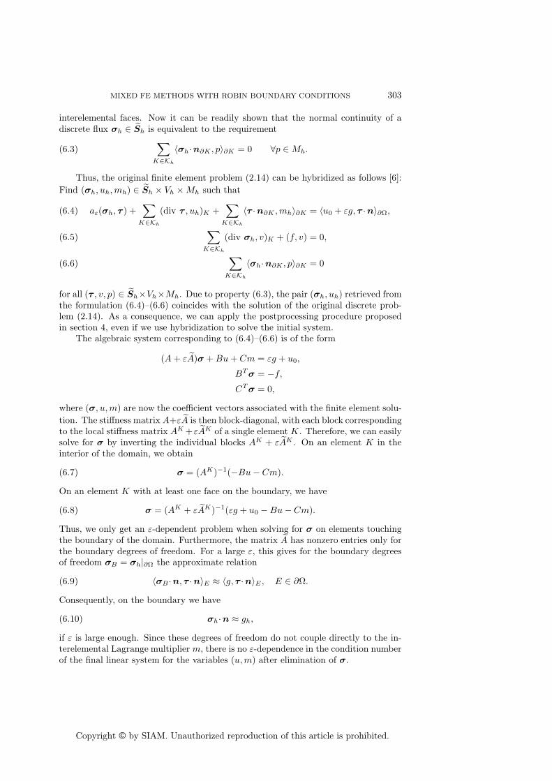
Copyright © by SIAM. Unauthorized reproduction of this article is prohibited.
MIXED FE METHODS WITH ROBIN BOUNDARY CONDITIONS 303
interelemental faces. Now it can be readily shown that the normal continuity of adiscrete flux σh ∈ Sh is equivalent to the requirement
(6.3)∑
K∈Kh
〈σh·n∂K , p〉∂K = 0 ∀p ∈ Mh.
Thus, the original finite element problem (2.14) can be hybridized as follows [6]:Find (σh, uh, mh) ∈ Sh × Vh × Mh such that
aε(σh, τ ) +∑
K∈Kh
(div τ , uh)K +∑
K∈Kh
〈τ ·n∂K , mh〉∂K = 〈u0 + εg, τ ·n〉∂Ω,(6.4)
∑K∈Kh
(div σh, v)K + (f, v) = 0,(6.5)
∑K∈Kh
〈σh·n∂K , p〉∂K = 0(6.6)
for all (τ , v, p) ∈ Sh×Vh×Mh. Due to property (6.3), the pair (σh, uh) retrieved fromthe formulation (6.4)–(6.6) coincides with the solution of the original discrete prob-lem (2.14). As a consequence, we can apply the postprocessing procedure proposedin section 4, even if we use hybridization to solve the initial system.
The algebraic system corresponding to (6.4)–(6.6) is of the form
(A + εA)σ + Bu + Cm = εg + u0,
BT σ = −f,
CT σ = 0,
where (σ, u, m) are now the coefficient vectors associated with the finite element solu-tion. The stiffness matrix A+εA is then block-diagonal, with each block correspondingto the local stiffness matrix AK +εAK of a single element K. Therefore, we can easilysolve for σ by inverting the individual blocks AK + εAK . On an element K in theinterior of the domain, we obtain
(6.7) σ = (AK)−1(−Bu − Cm).
On an element K with at least one face on the boundary, we have
σ = (AK + εAK)−1(εg + u0 − Bu − Cm).(6.8)
Thus, we only get an ε-dependent problem when solving for σ on elements touchingthe boundary of the domain. Furthermore, the matrix A has nonzero entries only forthe boundary degrees of freedom. For a large ε, this gives for the boundary degreesof freedom σB = σh|∂Ω the approximate relation
(6.9) 〈σB·n, τ ·n〉E ≈ 〈g, τ ·n〉E , E ∈ ∂Ω.
Consequently, on the boundary we have
(6.10) σh·n ≈ gh,
if ε is large enough. Since these degrees of freedom do not couple directly to the in-terelemental Lagrange multiplier m, there is no ε-dependence in the condition numberof the final linear system for the variables (u, m) after elimination of σ.
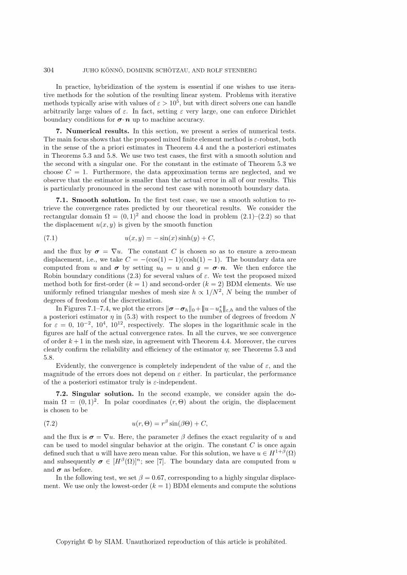
Copyright © by SIAM. Unauthorized reproduction of this article is prohibited.
304 JUHO KONNO, DOMINIK SCHOTZAU, AND ROLF STENBERG
In practice, hybridization of the system is essential if one wishes to use itera-tive methods for the solution of the resulting linear system. Problems with iterativemethods typically arise with values of ε > 105, but with direct solvers one can handlearbitrarily large values of ε. In fact, setting ε very large, one can enforce Dirichletboundary conditions for σ·n up to machine accuracy.
7. Numerical results. In this section, we present a series of numerical tests.The main focus shows that the proposed mixed finite element method is ε-robust, bothin the sense of the a priori estimates in Theorem 4.4 and the a posteriori estimatesin Theorems 5.3 and 5.8. We use two test cases, the first with a smooth solution andthe second with a singular one. For the constant in the estimate of Theorem 5.3 wechoose C = 1. Furthermore, the data approximation terms are neglected, and weobserve that the estimator is smaller than the actual error in all of our results. Thisis particularly pronounced in the second test case with nonsmooth boundary data.
7.1. Smooth solution. In the first test case, we use a smooth solution to re-trieve the convergence rates predicted by our theoretical results. We consider therectangular domain Ω = (0, 1)2 and choose the load in problem (2.1)–(2.2) so thatthe displacement u(x, y) is given by the smooth function
(7.1) u(x, y) = − sin(x) sinh(y) + C,
and the flux by σ = ∇u. The constant C is chosen so as to ensure a zero-meandisplacement, i.e., we take C = −(cos(1) − 1)(cosh(1) − 1). The boundary data arecomputed from u and σ by setting u0 = u and g = σ·n. We then enforce theRobin boundary conditions (2.3) for several values of ε. We test the proposed mixedmethod both for first-order (k = 1) and second-order (k = 2) BDM elements. We useuniformly refined triangular meshes of mesh size h ∝ 1/N2, N being the number ofdegrees of freedom of the discretization.
In Figures 7.1–7.4, we plot the errors ‖σ−σh‖0+ |||u−u∗h|||ε,h and the values of the
a posteriori estimator η in (5.3) with respect to the number of degrees of freedom Nfor ε = 0, 10−2, 104, 1012, respectively. The slopes in the logarithmic scale in thefigures are half of the actual convergence rates. In all the curves, we see convergenceof order k +1 in the mesh size, in agreement with Theorem 4.4. Moreover, the curvesclearly confirm the reliability and efficiency of the estimator η; see Theorems 5.3 and5.8.
Evidently, the convergence is completely independent of the value of ε, and themagnitude of the errors does not depend on ε either. In particular, the performanceof the a posteriori estimator truly is ε-independent.
7.2. Singular solution. In the second example, we consider again the do-main Ω = (0, 1)2. In polar coordinates (r, Θ) about the origin, the displacementis chosen to be
(7.2) u(r, Θ) = rβ sin(βΘ) + C,
and the flux is σ = ∇u. Here, the parameter β defines the exact regularity of u andcan be used to model singular behavior at the origin. The constant C is once againdefined such that u will have zero mean value. For this solution, we have u ∈ H1+β(Ω)and subsequently σ ∈ [Hβ(Ω)]n; see [7]. The boundary data are computed from uand σ as before.
In the following test, we set β = 0.67, corresponding to a highly singular displace-ment. We use only the lowest-order (k = 1) BDM elements and compute the solutions

Copyright © by SIAM. Unauthorized reproduction of this article is prohibited.
MIXED FE METHODS WITH ROBIN BOUNDARY CONDITIONS 305
103
104
105
106
107
10−20
10−15
10−10
10−5
Number of degrees of freedom
Err
or
Estimator, BDM1True error, BDM1Estimator, BDM2True error, BDM2
Fig. 7.1. Convergence of the smooth so-lution with ε = 0.
103
104
105
106
107
10−20
10−15
10−10
10−5
Number of degrees of freedom
Err
or
Estimator, BDM1True error, BDM1Estimator, BDM2True error, BDM2
Fig. 7.2. Convergence of the smooth so-lution with ε = 10−2.
103
104
105
106
107
10−20
10−15
10−10
10−5
Number of degrees of freedomE
rror
Estimator, BDM1True error, BDM1Estimator, BDM2True error, BDM2
Fig. 7.3. Convergence of the smooth so-lution with ε = 104.
103
104
105
106
107
10−20
10−15
10−10
10−5
Number of degrees of freedom
Err
or
Estimator, BDM1True error, BDM1Estimator, BDM2True error, BDM2
Fig. 7.4. Convergence of the smooth so-lution with ε = 1012.
on adaptively refined meshes for various values of ε. To create the mesh sequences,we have chosen to refine all elements in which the elemental indicator exceeds 30 per-cent of the maximal value. Contribution from an individual face estimator is dividedevenly to the elements sharing the face. To ensure sufficient refinement, we furtherhalve the refinement threshold until at least 10 percent of all elements are refined.For comparison, the computations are also performed using uniform mesh refinementwith an equivalent number of degrees of freedom. In Figures 7.5–7.8, we show theerrors ‖σ − σh‖0 + |||u − u∗
h|||ε,h and the values of the estimator η obtained for thisproblem with the values ε = 0, 10−2, 104, and 108.
In the case of uniform mesh refinement, the convergence rates are now limitedby the regularity of the solution. They are of the order hβ as expected. On theother hand, the adaptive mesh refinement strategy clearly is able to retrieve theconvergence to some extent. More importantly, even for the irregular boundary dataconsidered here, both the a priori and a posteriori estimates are observed to remainfully ε-independent, thus confirming the theoretical results.
The singularity of the solution in (7.2) lies in the origin and we expect the adap-tive meshes to be strongly refined into this corner. To ascertain the ε-independenceof the adaptive refinement procedure, we plot the mesh densities for different val-

Copyright © by SIAM. Unauthorized reproduction of this article is prohibited.
306 JUHO KONNO, DOMINIK SCHOTZAU, AND ROLF STENBERG
103
104
105
106
107
10−8
10−7
10−6
10−5
10−4
10−3
10−2
Number of degrees of freedom
Err
or
Estimator, adaptiveTrue error, adaptiveEstimator, uniformTrue error, uniform
Fig. 7.5. Convergence of the singularsolution with ε = 0.
103
104
105
106
107
10−8
10−7
10−6
10−5
10−4
10−3
10−2
Number of degrees of freedom
Err
or
Estimator, adaptiveTrue error, adaptiveEstimator, uniformTrue error, uniform
Fig. 7.6. Convergence of the singularsolution with ε = 10−2.
103
104
105
106
107
10−8
10−7
10−6
10−5
10−4
10−3
10−2
Number of degrees of freedomE
rror
Estimator, adaptiveTrue error, adaptiveEstimator, uniformTrue error, uniform
Fig. 7.7. Convergence of the singularsolution with ε = 104.
103
104
105
106
107
10−8
10−7
10−6
10−5
10−4
10−3
10−2
Number of degrees of freedom
Err
or
Estimator, adaptiveTrue error, adaptiveEstimator, uniformTrue error, uniform
Fig. 7.8. Convergence of the singularsolution with ε = 108.
0 0.5 10
0.2
0.4
0.6
0.8
1
First refinement
0
0.2
0.4
0.6
0.8
1
1.2
0 0.5 10
0.2
0.4
0.6
0.8
1
After 7 refinements
0
1
2
3
Fig. 7.9. Mesh density after one step, in the middle of the refinement procedure, and on thefinal mesh with ε = 0.
ues of the parameter ε at different stages of the refinement procedure. The plotsare normalized with respect to the largest element size (i.e., the largest element sizeequals unity) and are shown using a logarithmic scale.
From Figures 7.9–7.11, we see that our adaptive mesh refinement procedure clearlyyields equivalent mesh density distributions for different values of ε. This is what isdesired for this problem, since the refinement should only be driven by the irregularity
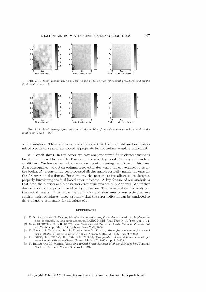
Copyright © by SIAM. Unauthorized reproduction of this article is prohibited.
MIXED FE METHODS WITH ROBIN BOUNDARY CONDITIONS 307
0 0.5 10
0.2
0.4
0.6
0.8
1
First refinement
0
0.2
0.4
0.6
0.8
1
1.2
0 0.5 10
0.2
0.4
0.6
0.8
1
After 7 refinements
1
2
3
4
Fig. 7.10. Mesh density after one step, in the middle of the refinement procedure, and on thefinal mesh with ε = 1.
0 0.5 10
0.2
0.4
0.6
0.8
1
First refinement
0
0.2
0.4
0.6
0.8
1
1.2
0 0.5 10
0.2
0.4
0.6
0.8
1
After 7 refinements
1
2
3
4
Fig. 7.11. Mesh density after one step, in the middle of the refinement procedure, and on thefinal mesh with ε = 104.
of the solution. These numerical tests indicate that the residual-based estimatorsintroduced in this paper are indeed appropriate for controlling adaptive refinement.
8. Conclusions. In this paper, we have analyzed mixed finite element methodsfor the dual mixed form of the Poisson problem with general Robin-type boundaryconditions. We have extended a well-known postprocessing technique to this case.As a consequence, we obtain optimal error estimates where the convergence rates forthe broken H1-errors in the postprocessed displacements correctly match the ones forthe L2-errors in the fluxes. Furthermore, the postprocessing allows us to design aproperly functioning residual-based error indicator. A key feature of our analysis isthat both the a priori and a posteriori error estimates are fully ε-robust. We furtherdiscuss a solution approach based on hybridization. The numerical results verify ourtheoretical results. They show the optimality and sharpness of our estimates andconfirm their robustness. They also show that the error indicator can be employed todrive adaptive refinement for all values of ε.
REFERENCES
[1] D. N. Arnold and F. Brezzi, Mixed and nonconforming finite element methods: Implementa-tion, postprocessing and error estimates, RAIRO Model. Anal. Numer., 19 (1985), pp. 7–32.
[2] S. C. Brenner and L. R. Scott, The Mathematical Theory of Finite Element Methods, 3rded., Texts Appl. Math. 15, Springer, New York, 2008.
[3] F. Brezzi, J. Douglas, Jr., R. Duran, and M. Fortin, Mixed finite elements for secondorder elliptic problems in three variables, Numer. Math., 51 (1987), pp. 237–250.
[4] F. Brezzi, J. Douglas, Jr., and L. D. Marini, Two families of mixed finite elements forsecond order elliptic problems, Numer. Math., 47 (1985), pp. 217–235.
[5] F. Brezzi and M. Fortin, Mixed and Hybrid Finite Element Methods, Springer Ser. Comput.Math. 15, Springer-Verlag, New York, 1991.
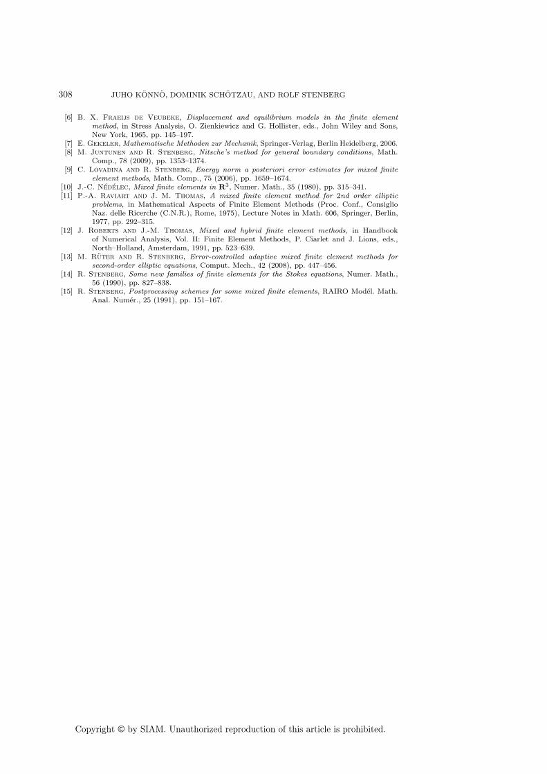
Copyright © by SIAM. Unauthorized reproduction of this article is prohibited.
308 JUHO KONNO, DOMINIK SCHOTZAU, AND ROLF STENBERG
[6] B. X. Fraeijs de Veubeke, Displacement and equilibrium models in the finite elementmethod, in Stress Analysis, O. Zienkiewicz and G. Hollister, eds., John Wiley and Sons,New York, 1965, pp. 145–197.
[7] E. Gekeler, Mathematische Methoden zur Mechanik, Springer-Verlag, Berlin Heidelberg, 2006.[8] M. Juntunen and R. Stenberg, Nitsche’s method for general boundary conditions, Math.
Comp., 78 (2009), pp. 1353–1374.[9] C. Lovadina and R. Stenberg, Energy norm a posteriori error estimates for mixed finite
element methods, Math. Comp., 75 (2006), pp. 1659–1674.[10] J.-C. Nedelec, Mixed finite elements in R3, Numer. Math., 35 (1980), pp. 315–341.[11] P.-A. Raviart and J. M. Thomas, A mixed finite element method for 2nd order elliptic
problems, in Mathematical Aspects of Finite Element Methods (Proc. Conf., ConsiglioNaz. delle Ricerche (C.N.R.), Rome, 1975), Lecture Notes in Math. 606, Springer, Berlin,1977, pp. 292–315.
[12] J. Roberts and J.-M. Thomas, Mixed and hybrid finite element methods, in Handbookof Numerical Analysis, Vol. II: Finite Element Methods, P. Ciarlet and J. Lions, eds.,North–Holland, Amsterdam, 1991, pp. 523–639.
[13] M. Ruter and R. Stenberg, Error-controlled adaptive mixed finite element methods forsecond-order elliptic equations, Comput. Mech., 42 (2008), pp. 447–456.
[14] R. Stenberg, Some new families of finite elements for the Stokes equations, Numer. Math.,56 (1990), pp. 827–838.
[15] R. Stenberg, Postprocessing schemes for some mixed finite elements, RAIRO Model. Math.Anal. Numer., 25 (1991), pp. 151–167.

Publication II
Juho Könnö and Rolf Stenberg. Analysis of H(div)-conforming FiniteElements for the Brinkman Problem. Accepted for publication inMathematical Models and Methods in Applies Sciences, doi:10.1142/S0218202511005726, 2011.
c© 2011 World Scientific Publishing Company.Reprinted with permission.
59


January 27, 2011 9:23 WSPC/INSTRUCTION FILE brink3
H(div)-CONFORMING FINITE ELEMENTS FOR THE
BRINKMAN PROBLEM
JUHO KÖNNÖ
Department of Mathematics and Systems Analysis, Aalto University
PO Box 11100, 00076 Aalto, Finland
ROLF STENBERG
Department of Mathematics and Systems Analysis, Aalto University
PO Box 11100, 00076 Aalto, Finland
rolf.stenberg@tkk.
Received (Day Month Year)Revised (Day Month Year)
Communicated by (xxxxxxxxxx)
The Brinkman equations describe the ow of a viscous uid in a porous matrix. Mathe-matically the Brinkman model is a parameter-dependent combination of both the Darcyand Stokes models. We introduce a dual mixed framework for the problem, and useH(div)-conforming nite elements with the SIPG method to obtain a stable formula-tion. We show the formulation to be stable in a mesh-dependent norm for all values ofthe parameter. We also introduce a postprocessing scheme for the pressure along with aresidual-based a posteriori estimator, which is shown to be ecient and reliable for allparameter values.
Keywords: Brinkman problem, H(div)-conforming, postprocessing, a posteriori error es-timates, SIPG, Nitsche's method, Darcy-Stokes equation
AMS Subject Classication: 65N15,65N30
1. Introduction
In soil mechanics, the Brinkman equation describes the ow of a viscous uid in
a very porous medium. For a derivation of and details on the equations we refer
to Refs. 21, 1, 2, 3, and 25. As opposed to the Darcy model widely used in soil
mechanics, the Brinkman model adds an eective viscosity term into the equations.
Typical applications of the equations lie in oil exploration, groundwater modelling,
and some special applications, such as heat pipes19. The Brinkman model is also
often used as a coupling layer between a free surface ow and a porous Darcy ow12.
Mathematically, the Brinkman equations are a parameter-dependent combination
of the Darcy and Stokes equations.
We study the application of H(div)-conforming nite elements designed for the
Darcy problem to the more complicated Brinkman problem. H(div)-elements have
1
January 27, 2011 9:23 WSPC/INSTRUCTION FILE brink3
2
been considered for the closely related Stokes problem in Refs. 10, 35, 18, and 36.
Stokes-based nite element methods for the Brinkman problem are studied e.g. in
Refs. 16, 6, 11, and 37. In Ref.11 the coupling of Darcy, Stokes, and Brinkman ows
using an interior penalty method is studied with extensive a priori results. Our
model constitutes an approximation with non-conforming basis functions, since in
the discretizations of the H(div)-space only the normal component of the veloc-
ity is continuous on interelement boundaries. To enforce the tangential continuity,
we use a symmetric interior penalty Galerkin (SIPG) method rst introduced for
enforcing boundary conditions by Nitsche,24 which in turn requires the use of a
mesh-dependent bilinear form. Sometimes the method is also referred to as Nitsche's
method. The H(div)-conforming approach has been considered for the Brinkman
ow in Ref. 37 by modifying the standard Darcy elements with additional degrees
of freedom. The interior penalty formulation is considered in Ref. 15, but no error
estimates are given. The method has a strong resemblance to the totally discontinu-
ous Galerkin methods for the Stokes equation, cf. Ref 14. The motivation for using
this non-conforming approximation is the fact, that H(div)-conforming elements
are widely used in industry for solving the Darcy equation, and we want to derive
a way of easily incorporating viscosity to the existing solvers, along with a rigorous
mathematical analysis.
In this paper, we present a comprehensive error analysis with both a priori and a
posteriori estimates in parameter dependent norms valid for all values of the eective
viscosity parameter. As opposed to the analysis in Ref. 37, we use the standard
H(div)-conforming nite element spaces with no additional degrees of freedom. In
Ref. 36 these elements are studied for the Stokes problem with a priori estimates in
H1×L2. Similar ideas are used in Ref. 17 for coupling a Stokes and a Darcy ow with
a Nitsche-type method, and an a priori analysis is presented. Our work combines the
aforementioned results forH(div)-conforming approximations of the Stokes problem
via SIPG techniques with the analysis of the Darcy equation in Ref. 22. A priori
convergence results are given in a mesh-dependent norm, the type of which changes
with the parameter value from the natural norm for the Stokes problem to the
energy-norm equivalent for the Darcy pressure, namely the L2-norm for the velocity
and the broken H1-norm for the pressure. We also present a postprocessing scheme
for the pressure which allows us to obtain optimal-order convergence in the whole
of the parameter range. A residual-based sharp and reliable a posteriori estimator
fully robust in the parameter t is introduced, which to our knowledge has not been
done before for the Brinkman problem. We further emphasize the fact, that all of
the constants in the analysis are independent of the mesh size and the parameter
t, and the method works for all parameter values 0 ≤ t <∞.
The structure of the article is as follows. First, we formulate the Brinkman
problem mathematically and introduce the corresponding variational formulation.
Then we introduce the nite element spaces used for the discretization along with
the mesh-dependent energy norms in which the error is measured. We derive a
priori convergence results for this discretization, which implies the possibility of

January 27, 2011 9:23 WSPC/INSTRUCTION FILE brink3
3
improving the accuracy of the pressure approximation via postprocessing. This is
addressed in a separate chapter, in which we provide optimal a priori convergence
results for the postprocessed solution. Finally, we end the paper with the a posteriori
error analysis. A residual-based a posteriori error estimator is introduced. It is then
shown, that the estimator is both reliable and ecient for all values of the viscosity
parameter.
We use standard notation throughout the paper. We denote by C,C1, C2 etc.
generic constants, that are not always identical in value, but are always independent
of the parameter t and the mesh size.
2. The Brinkman Model
Let Ω ⊂ Rn, with n = 2, 3 be a polygonal or polyhedral domain. We denote by
u the velocity eld of the uid and by p the pore pressure. The equations are
scaled as presented in Ref. 13, with the single parameter t representing the eective
viscosity of the uid, which is assumed constant for simplicity. Given the loadings
f ∈ [L2(Ω)]n and g ∈ L20(Ω), the Brinkman equations are
−t2∆u+ u+∇p = f , in Ω, (2.1) eq:strong
div u = g, in Ω. (2.2)
For t > 0, the equations are formally a Stokes problem. The solution (u, p) is
sought in V ×Q = [H10 (Ω)]n×L2
0(Ω). For the case t = 0 we get the Darcy problem,
and accordingly the solution space is V ×Q = H(div,Ω)×L20(Ω). For simplicity of
the mathematical analysis, we consider homogenous Dirichlet boundary conditions
for the velocity eld. Thus for the case t > 0 the boundary conditions are
u = 0. (2.3) eq:brinkbc
The correct boundary condition for the limiting Darcy case t = 0 is
u·n = 0. (2.4) eq:darcybc
In the following, we denote by (· , · )D the standard L2inner product over a set
D ⊂ Rn. If D = Ω, the subscript is dropped for convenience. Similarly, 〈· , · 〉B is
the L2inner product over a set B ⊂ Rn−1. We dene the following bilinear forms
a(u,v) = t2(∇u,∇v) + (u,v), (2.5)
b(v, p) = −(div v, p), (2.6)
and
B(u, p;v, q) = a(u,v) + b(v, p) + b(u, q). (2.7)
The weak formulation of the Brinkman problem then reads: Find (u, p) ∈ V × Qsuch that
B(u, p;v, q) = (f ,v)− (g, q), ∀(v, q) ∈ V ×Q. (2.8) eq:weakprob
January 27, 2011 9:23 WSPC/INSTRUCTION FILE brink3
4
In order for the SIPG method to be well-dened, we make the following regu-
larity assumption throughout our analysis.
Assumption 2.1 The solution of (2.8) satises tu ∈ [Hr(Ω)]n∩V , with r > 3/2.as:ureg
3. Solution by Mixed Finite Elements
Let Kh be a shape-regular partition of Ω into simplices. As usual, the diameter
of an element K is denoted by hK , and the global mesh size h is dened as h =maxK∈Kh
hK . We denote by Eh the set of all faces of Kh. We write hE for the
diameter of a face E. We refer to the boundaries of an element regardless of the
spatial dimension n colloquially as faces throughout the paper.
We introduce the jump and average of a piecewise smooth scalar function f as
follows. Let E = ∂K ∩ ∂K ′ be an interior face shared by two elements K and K ′.Then the jump of f over E is dened by
[[f ]] = f |K − f |K′ . (3.1) eq:jump
and the average as
f =12
(f |K + f |K′). (3.2) eq:average
For vector valued functions, we dene the jumps and averages analogously.
3.1. The mixed method and the norms
Mixed nite element discretization of the problem is based on nite element spaces
Vh×Qh ⊂ H(div,Ω)×L20(Ω) of piecewise polynomial functions with respect to Kh.
We will focus here on the Raviart-Thomas (RT) and Brezzi-Douglas-Marini (BDM)
families of elements.9 Other common choices of spaces are the BDFM elements8
and in three dimensions the BDDF elements.23 That is, for an approximation of
order k ≥ 1, the velocity space Vh is taken as one of the following two spaces
V RTh = v ∈ H(div,Ω) | v|K ∈ [Pk−1(K)]n ⊕ xPk−1(K) ∀K ∈ Kh, (3.3) def:vspace
V BDMh = v ∈ H(div,Ω) | v|K ∈ [Pk(K)]n ∀K ∈ Kh, (3.4) def:vspace_bdm
in which Pk−1(K) denotes the homogeneous polynomials of degree k− 1. The pres-sure is approximated in the space
Qh = q ∈ L20(Ω) | q|K ∈ Pk−1(K) ∀K ∈ Kh. (3.5) def:qspace
Notice, that V RTh ⊂ V BDM
h and QBDMh = QRTh . The combination of spaces satises
the following equilibrium property:
div Vh ⊂ Qh. (3.6) eq:eqlprop
To ensure the stability of the non-conforming approximation, we use a symme-
teric interior penalty Nitsche-type method36,16,24 with a suitably chosen stabiliza-
tion parameter α. We dene the following mesh-dependent bilinear form
Bh(u, p;v, q) = ah(u,v) + b(v, p) + b(u, q), (3.7) def:hbilinear

January 27, 2011 9:23 WSPC/INSTRUCTION FILE brink3
5
in which
ah(u,v) = (u,v) + t2∑K∈Kh
(∇u,∇v)K (3.8) def:ahbilinear
+ t2∑E∈Eh
αhE〈[[u]], [[v]]〉E − 〈∂u
∂n, [[v]]〉E − 〈∂v
∂n, [[u]]〉E.
Then the discrete problem reads: Find uh ∈ Vh and ph ∈ Qh such that
Bh(uh, ph;v, q) = (f ,v)− (g, q), ∀(v, q) ∈ Vh ×Qh. (3.9) eq:feproblem
We introduce the following mesh-dependent norms for the problem. For the
velocity we use
‖u‖2t,h = ‖u‖2 + t2
( ∑K∈Kh
‖∇u‖20,K +∑E∈Eh
1hE‖[[u· τ ]]‖20,E
), (3.10) def:uhnorm
and for the pressure
|||p|||2t,h =∑K∈Kh
h2K
h2K + t2
‖∇p‖20,K +∑E∈Eh
hEh2E + t2
‖[[p]]‖20,E . (3.11) def:phnorm
Note, that both of the norms are also parameter dependent. In the following, the
standard Sobolev norm of order k is denoted ‖· ‖k.
3.2. Interpolation in H(div)
For interpolation in H(div), a special interpolation operator is required. We use
the classical interpolation operator Rh : H(div,Ω)⋂
[Ls(Ω)]n → Vh with s > 2for dual mixed methods, cf. Refs. 9 and 33. We denote by Ph : L2(Ω) → Qh the
L2-projection. Employing integration by parts and the denition of the interpolant,
the interpolation operator satises the relation
(div (v −Rhv), q) = 0, ∀q ∈ Qh. (3.12) eq:divinter
The interpolant also satises the following properties. The equilibrium prop-
erty (3.6) implies
(div v, q − Phq) = 0, ∀v ∈ Vh. (3.13) eq:intl2prop
Furthermore, we have the commuting diagram property:
div Rh = Phdiv. (3.14) eq:comdiaprop
Remark 3.1. Note, that some additional regularity is required from the velocity
space for the interpolation operator to be well-dened. Due to Assumption 2.1 it
holds by the Sobolev embedding theorem that u ∈ [Ls(Ω)]n for every s ≥ 2 and
thus the interpolant Rh is well-dened.
January 27, 2011 9:23 WSPC/INSTRUCTION FILE brink3
6
3.3. A priori analysis
First we show that the formulation (3.9) gives a consistent method.
Lemma 3.1. Let the regularity of Assumption 2.1 hold. Then the exact solutionth:cons
(u, p) ∈ V ×Q satises
Bh(u, p;v, q) = (f ,v)− (g, q), ∀(v, q) ∈ Vh ×Qh. (3.15)
Proof. For the exact solution (u, p) the jumps on the interelement boundaries
vanish. Thus inserting (u, p) into the modied bilinear form Bh, we have using
Green's formula
Bh(u, p;v, q) = (u,v) + t2
( ∑K∈Kh
(∇u,∇v)K −∑E∈Eh
〈∂u∂n, [[v]]〉E
)− (div v, p)− (div u, q)
= (u,v) + t2∑K∈Kh
(∇u,∇v)K − 〈∂u∂n
,v〉∂K+ (∇p,v)− (g, q)
= (f ,v)− (g, q).
Recall, that the normal derivative can be estimated as31
hE‖∂v∂n‖20,E ≤ CI‖∇v‖20,K , ∀v ∈ Vh. (3.16) eq:normalapp
We then state the stability of ah(· , · ) in the mesh-dependent norm (3.10). The
stability only holds in the discrete space Vh. For a proof of the following lemma, cf.
Ref. 4.
Lemma 3.2. Let α > CI/2, with CI from (3.16). Then the bilinear form ah(· , · )is coercive in the discrete space Vh with a positive constant C such that
ah(v,v) ≥ C‖v‖2t,h, ∀v ∈ Vh. (3.17) res:a-stab
Next, we prove the discrete Brezzi-Babu²ka stability condition for the chosen
discretization of the Brinkman model. Recall, that we only have to prove the con-
dition in the Raviart-Thomas case since V RTh ⊂ V BDM
h . The following lemma is
an extension of the results presented in Ref. 26 for the mesh dependent norms27,28,
and in Refs. 36 and 10 for the Stokes equation with similar norms.
Lemma 3.3. There exists a positive constant C such thatlm:bbcond
supv∈Vh
b(v, q)‖v‖t,h ≥ C|||q|||t,h, ∀q ∈ Qh. (3.18) eq:bbcond
Proof. We recall that the local degrees of freedom for the RT family are
〈v·n, z〉E , ∀z ∈ Pk−1(E), (3.19)
(v, z)K , ∀z ∈ [Pk−2(K)]n. (3.20)
January 27, 2011 9:23 WSPC/INSTRUCTION FILE brink3
7
Thus, for a given q ∈ Qh we dene v to satisfy
〈v·n, z〉E = − hKh2K + t2
〈[[q]], z〉E , ∀z ∈ Pk−1(E), (3.21) def:infsupcond
(v, z)K =h2K
h2K + t2
(∇q, z)K ∀z ∈ [Pk−2(K)]n.
Choosing z = [[q]] ∈ Pk−1(E) and z = ∇q ∈ [Pk−2(K)]n gives
〈v·n, [[q]]〉E = − hKh2K + t2
‖[[q]]‖20,E , (3.22)
(v,∇q)K =h2K
h2K + t2
‖∇q‖20,K . (3.23)
An explicit inspection of the degrees of freedom yields the relation
h2K + t2
h2K
‖v‖20,K ≤hK
h2K + t2
‖[[q]]‖20,E +h2K
h2K + t2
‖∇q‖20,K . (3.24)
Thus we have using scaling arguments
‖v‖2t,h ≤ Ch2K + t2
h2K
∑K∈Kh
‖v‖20,K ≤ C|||q|||2t,h. (3.25) eq:infsupalakerta
Next we use element-by-element partial integration on b(v, q), and apply the de-
nitions (3.21) to get
b(v, q) =∑K∈Kh
(v,∇q)K −∑E∈Eh
〈v·n, q〉E (3.26) eq:infsupylakerta
=∑K∈Kh
h2K
h2K + t2
(∇q,∇q)K +∑E∈Eh
hKh2K + t2
〈[[q]], [[q]]〉E (3.27)
= |||q|||2t,h. (3.28)
Combining (3.25) and (3.26) gives (3.18).
By the above stability results for ah(· , · ) and b(· , · ) the following stability resultholds.9
Lemma 3.4. For some positive constant C it holdslm:fullstab
sup(v,q)∈Vh×Qh
Bh(r, s;v, q)‖v‖t,h + |||q|||t,h ≥ C(‖r‖t,h + |||s|||t,h), ∀(r, s) ∈ Vh ×Qh. (3.29)
Now we are ready to present the main results of the chapter. First, we have the
following quasioptimal a priori result.
Theorem 3.1. Assume that Assumption 2.1 holds. Then there is a positive con-
stant C such that
‖u− uh‖t,h + |||Php− ph|||t,h ≤ C‖u−Rhu‖t,h. (3.30)

January 27, 2011 9:23 WSPC/INSTRUCTION FILE brink3
8
Proof. By Lemma 3.4 there exists functions (v, q) ∈ Vh × Qh such that
‖v‖t,h + |||q|||t,h ≤ C, and
‖uh −Rhu‖t,h + |||ph − Php|||t,h ≤ Bh(uh −Rhu, ph − Php;v, q)= ah(uh −Rhu,v)− (div v, ph − Php)− (div (uh −Rhu), q)
= ah(u−Rhu,v)− (div v, p− Php)− (div (u−Rhu), q), (3.31)
in which the last line follows from the consistency of the method given by
Lemma 3.1. By using the interpolation properties (3.12) and (3.13), we arrive at
‖uh −Rhu‖t,h + |||ph − Php|||t,h ≤ ah(u−Rhu,v) ≤ C‖u−Rhu‖t,h (3.32)
Using the triangle inequality yields the result of the theorem.
We conclude the chapter with the following theorem, which shows that anal-
ogously to the dual mixed formulation of the Poisson problem5,30,22, we have a
superconvergence result for |||ph − Php|||t,h. This implies that the pressure solution
can be improved by local postprocessing.
Theorem 3.2. Assuming u ∈ [Hk+1(Ω)]n or u ∈ [Hk(Ω)]n for BDM and RTth:apriori
elements of order k, respectively, we have
‖u− uh‖t,h + |||Php− ph|||t,h ≤C(hk + thk−1)‖u‖k, for RT,
C(hk+1 + thk)‖u‖k+1, for BDM.(3.33) eq:apriori
4. The Postprocessing Method
In this section we present a postprocessing method for the pressure in the spirit of
Refs. 30, 29, 32, and 22. We seek the postprocessed pressure in an augmented space
Q∗h ⊃ Qh, dened as
Q∗h =
q ∈ L2(Ω) | q|K ∈ Pk(K) ∀K ∈ Kh, for RT,
q ∈ L2(Ω) | q|K ∈ Pk+1(K) ∀K ∈ Kh, for BDM.(4.1)
The postprosessing method is: Find p∗h ∈ Q∗h such that
Php∗h = ph, (4.2)
(∇p∗h,∇q)K = (t2∆uh − uh + f ,∇q)K , ∀q ∈ (I − Ph)Q∗h|K . (4.3)
Remark 4.1. Note, that the new pressure approximation is completely determined
by the solution (uh, ph) on the original nite element spaces Vh × Qh, which sat-
isfy the Brezzi-Babu²ka stability condition intrinsically. By Theorem 3.2 we have
optimal order of convergence for the velocity eld even without postprocessing. Fur-
thermore, since the postprocessed pressure is computed elementwise the method is
computationally inexpensive and easy to implement.
January 27, 2011 9:23 WSPC/INSTRUCTION FILE brink3
9
For the purposes of mathematical analysis the method can be compactly treated
as an integral part of the problem by embedding it into the bilinear form. We
introduce the modied bilinear form
B∗h(u, p∗;v, q∗) = Bh(u, p∗;v, q∗) +∑K∈Kh
h2K
h2K + t2
(∇p∗+u− t2∆u,∇(I −Ph)q∗)K .
(4.4) def:ppbilin
The postprocessed problem is then: Find (uh, p∗h) ∈ Vh × Q∗h such that for every
pair (v, q∗) ∈ Vh ×Q∗h it holds
B∗h(uh, p∗h;v, q∗) = Lh(f , Phg;v, q∗), (4.5) eq:pp-problem
in which
Lh(f , g;v, q∗) = (f ,v)− (g, q∗) +∑K∈Kh
h2K
h2K + t2
(f ,∇(I − Ph)q∗)K . (4.6) def:loadfun
We have the following lemma extending the results of Lemma 2.4 of Ref. 22, which
relates the solution of the postprocessed problem to the original problem.
Lemma 4.1. Let (uh, p∗h) ∈ Vh × Q∗h be the solution of the problem (4.5) and set
ph = Php∗h. Then (uh, ph) ∈ Vh ×Qh is the solution of the original problem (3.9).
Conversely, if (uh, ph) ∈ Vh ×Qh is the solution of the original problem (3.9) and
p∗h is dened as above, then (uh, p∗h) ∈ Vh ×Q∗h is the solution to (4.5).
Proof. Testing with (v, 0) ∈ Vh ×Q∗h and using the equilibrium property yields
B∗h(uh, p∗h;v, 0) = ah(uh,v)− (div v, p∗h)
= ah(uh,v)− (div v, Php∗h)
= ah(uh,v)− (div v, ph) = (f ,v).
On the other hand, testing with (0, Phq∗) ∈ Vh ×Qh ⊂ Vh ×Q∗h gives
B∗h(uh, p∗h; 0, Phq∗) = −(div uh, Phq∗) = −(g, Phq∗).
Combining the above two equations yields the original problem (3.9) and rst part
of the assertion is proved. Next take (uh, ph) to be the solution of (3.9), and p∗hthe postprocessed pressure dened above. Using the denition of the postprocessed
January 27, 2011 9:23 WSPC/INSTRUCTION FILE brink3
10
pressure and the equilibrium property, we have
B∗h(uh, p∗h;v, q∗) = B∗h(uh, p∗h;v, Phq∗) + B∗h(uh, p∗h; 0, (I − Ph)q∗)
= ah(uh,v)− (div v, p∗h)− (div uh, Phq∗)
+∑K∈Kh
h2K
h2K + t2
(−t2∆uh + uh +∇p∗h,∇(I − Ph)Phq∗)K
− (div uh, (I − Ph)q∗) +∑K∈Kh
h2K
h2K + t2
(f ,∇(I − Ph)2q∗)K
+h2K
h2K + t2
(−t2∆uh + uh +∇p∗h − f ,∇(I − Ph)2q∗)K
= ah(uh,v)− (div v, Php∗h)− (div uh, Phq∗)
− (div uh, Ph(I − Ph)q∗) +∑K∈Kh
h2K
h2K + t2
(f ,∇(I − Ph)2q∗)K
= Lh(f , Phg;v, q∗)
for arbritrary (v, q∗) ∈ Vh ×Q∗h. Thus the second part of the assertion is valid.
Next we show that the postprocessed method is stable in the discrete spaces.
For this we need the following lemma.22
Lemma 4.2. There exists positive constants C1, C2 such that for every q∗ ∈ Q∗h it
holds
|||q∗|||t,h ≤ |||Phq∗|||t,h + |||(I − Ph)q∗|||t,h ≤ C2|||q∗|||t,h, (4.7) eq:ppnormeq1
C1|||q∗|||t,h ≤ |||Phq∗|||t,h +
( ∑K∈Kh
‖∇(I − Ph)q∗‖20,K)1/2
≤ C2|||q∗|||t,h. (4.8) eq:ppnormeq2
Since (I − Ph)q∗ is L2-orthogonal to piecewise constant functions, we furthermore
have the following estimate with C3 > 0:
|||(I − Ph)q∗|||t,h ≤ C3
( ∑K∈Kh
‖∇(I − Ph)q∗‖20,K)1/2
. (4.9) eq:ppnormeq3
We are now ready to prove the main stability result.
Lemma 4.3. There exists C > 0 such that for every (u, p∗) ∈ Vh ×Q∗h it holdsth:ppstab
sup(v,q∗)∈Vh×Q∗h
B∗h(u, p∗;v, q∗)‖v‖t,h + |||q∗|||t,h ≥ C(‖u‖t,h + |||p∗|||t,h). (4.10)
Proof. Let (u, p∗) ∈ Vh ×Q∗h be arbitrary. Choosing q∗ = q ∈ Qh we have
B∗h(u, p∗;v, q) = ah(u,v)− (div v, p∗)− (div u, q)
= ah(u,v)− (div v, Php∗)− (div u, q)
= Bh(u, Php∗;v, q).
January 27, 2011 9:23 WSPC/INSTRUCTION FILE brink3
11
Thus Lemma 3.4 guarantees that there exists (v, q) ∈ Vh ×Qh such that ‖v‖t,h +|||q|||t,h ≤ C(‖u‖t,h + |||Php∗|||t,h) and
Bh(u, p∗;v, q) ≥ C(‖u‖t,h + |||Php∗|||t,h). (4.11) apu:partialstab
Next, we choose (v, q∗) = (0, (I − Ph)p∗) ∈ Vh ×Q∗h. This gives
B∗h(u, p∗; 0, (I − Ph)p∗)
= −(div u, (I − Ph)p∗) +∑K∈Kh
h2K
h2K + t2
(∇p∗ + u− t2∆u,∇(I − Ph)p∗)K
≥ −C(‖u‖t,h|||(I − Ph)p∗|||t,h) +∑K∈Kh
h2K
h2K + t2
‖∇(I − Ph)p∗‖20,K
+∑K∈Kh
h2K
h2K + t2
(∇Php∗ + u− t2∆u,∇(I − Ph)p∗)K
≥ −C(‖u‖t,h + |||Php∗|||t,h)|||(I − Ph)p∗|||t,h +∑K∈Kh
h2K
h2K + t2
‖∇(I − Ph)p∗‖20,K
−( ∑K∈Kh
h2K
h2K + t2
‖t2∆u‖20,K)1/2
|||(I − Ph)p∗|||t,h.
We can estimate the term containing the Laplacian using the inverse inequality as
follows:∑K∈Kh
h2K
h2K + t2
‖t2∆u‖20,K ≤∑K∈Kh
t2h2K
h2K + t2
1h2K
‖t∇u‖20,K ≤ t2∑K∈Kh
‖∇u‖20,K .
Using Young's inequality and the norm equivalence (4.9), we have for any ε > 0
B∗h(u, p∗; 0, (I − Ph)p∗) ≥ −C1
2ε(‖u‖t,h + |||Php∗|||t,h)2 − ε
2|||(I − Ph)p∗|||2t,h
+∑K∈Kh
h2K
h2K + t2
‖∇(I − Ph)p∗‖20,K
≥ −C1
2ε(‖u‖t,h + |||Php∗|||t,h)2
+
(1− C2ε
2
) ∑K∈Kh
h2K
h2K + t2
‖∇(I − Ph)p∗‖20,K .
Choosing ε = 1/C1 yields, with C3 = C1C2/2, the estimate
B∗h(u, p∗; 0, (I − Ph)p∗) ≥ −C3(‖u‖t,h + |||Php∗|||t,h)2
+12
∑K∈Kh
h2K
h2K + t2
‖∇(I − Ph)p∗‖20,K . (4.12) apu:partialstab2

January 27, 2011 9:23 WSPC/INSTRUCTION FILE brink3
12
Combining estimates (4.11) and (4.12), the norm equivalence (4.8), and choosing δ
suciently small, we have
B∗h(u, p∗;v, q + δ(I − Ph)p∗) ≥ (1− δC3)(‖u‖t,h + |||Php∗|||t,h)2
δC3
∑K∈Kh
‖∇(I − Ph)p∗‖20,K
≥ C(‖u‖t,h + |||p∗|||t,h)2.
Furthermore,
‖v‖t,h + |||q + δ(I − Ph)p∗|||t,h ≤ ‖v‖t,h + |||q|||t,h + δ|||(I − Ph)p∗|||t,h≤ C(‖u‖t,h + |||Php∗|||t,h) + δ|||(I − Ph)p∗|||t,h≤ C(‖u‖t,h + |||p∗|||t,h),
giving the desired result.
We have the following a priori results, which show that given sucient regularity,
the postprocessed displacement converges with an optimal rate.
Theorem 4.1. Assume Assumption 2.1 holds. Then for the postprocessed solutionth:ppapriori
(uh, p∗h) it holds
‖u− uh‖t,h + |||p− p∗h|||t,h ≤ C infq∗∈Q∗h
‖u−Rhu‖t,h + |||p− q∗|||t,h
+ (∑K∈Kh
h2K
h2K + t2
‖∇q∗ +Rhu− t2∆Rhu− f‖20,K)1/2. (4.13)
Proof. Let q∗ ∈ Q∗h. From Lemma 4.3 it follows that we have a pair (v, r∗) ∈Vh ×Q∗h such that ‖v‖t,h + |||r∗|||t,h ≤ C and
‖uh −Rhu‖t,h + |||p∗h − q∗|||t,h ≤ CB∗h(uh −Rhu, p∗h − q∗;v, r∗).
Combining the denition of the postprocessed problem and the consistency re-
sult 3.1 gives
‖uh −Rhu‖t,h + |||p∗h − q∗|||t,h ≤ CB∗h(u−Rhu, p− q∗;v, r∗) + (g − Phg, r∗)= ah(u−Rhu,v)− (div v, p− q∗)− (div (u−Rhu), r∗) + (g − Phg, r∗)
+∑K∈Kh
h2K
h2K + t2
(∇(p− q∗) + (u−Rhu)− t2∆(u−Rhu),∇(I − Ph)r∗)K .
The last two terms on the second line cancel by the commuting diagram prop-
erty (3.14). Inserting f into the last equation we have
‖uh −Rhu‖t,h + |||p∗h − q∗|||t,h ≤ C‖u−Rhu‖t,h‖v‖t,h + |||p− q∗|||t,h‖v‖t,h+ (
∑K∈Kh
h2K
h2K + t2
‖∇q∗ +Rhu− t2∆Rhu− f‖20,K)1/2|||r∗|||t,h.
January 27, 2011 9:23 WSPC/INSTRUCTION FILE brink3
13
Thus the assertion is proved using the triangle equality and the above result.
Assuming full regularity, we have the following optimal a priori result for the
postprocessed problem.
Theorem 4.2. Let us assume (u, p) ∈ [Hk+1(Ω)]n ×Hk+2(Ω) or u ∈ [Hk(Ω)]n ××Hk+1(Ω) for BDM and RT elements of order k, respectively. Then we have for
the solution (uh, p∗h) of the postprocessed problem (4.5)
‖u−uh‖t,h+|||p−p∗h|||t,h ≤C(h+ t)hk−1‖u‖k + (h+ t)−1hk+1‖p‖k+1, for RT,
C(h+ t)hk‖u‖k+1 + (h+ t)−1hk+2‖p‖k+2, for BDM.
Remark 4.2. Clearly, as t ≤ h we recover the converge rates hk and hk+1 for the
RT and BDM elements, respectively, as expected for the Darcy equation.22 Similarly,
when t h we are in the Stokes regime and recover a convergence rate of hk−1
and hk for the method with RT and BDM elements, in accordance with the results
in Refs. 36, 17 and 10. Note, that in the Stokes regime the regularity assumption
for the pressure is unnecessarily restrictive. For the aforementioned converge rates
to hold for t h, we only have to assume p ∈ Hk−1(Ω) or p ∈ Hk(Ω) for RT and
BDM elements of order k.
5. A Posteriori Estimates
In this section we derive a residual-based a posteriori estimator for the postpro-
cessed solution. It should be noted, that the postprocessing is vital for a properly
functioning estimator. Our derivation of the a posteriori estimator is based on the
following saturation assumption.7,22
Assumption 5.1 Let Kh/2 be a uniformly rened subtriangulation of Kh. Thenas:saturationthere is a constant β < 1 such that
‖u− uh/2‖t,h/2 + |||p− p∗h/2|||t,h/2 ≤ β(‖u− uh‖t,h + |||p− p∗h|||t,h). (5.1)
The triangle inequality gives the following more useful form for the saturation
assumption.
‖u− uh‖t,h + |||p− p∗h|||t,h ≤1
1− β (‖uh/2 − uh‖t,h/2 + |||p∗h/2 − p∗h|||t,h/2). (5.2) eq:saturation_apu
We divide the estimator into two distinct parts, one dened over the elements and
one over the faces of the mesh. The elementwise and facewise estimators are dened
as
η2K =
h2K
h2K + t2
‖ − t2∆uh + uh +∇p∗h − f‖20,K + (t2 + h2K)‖g − Phg‖20,K , (5.3) def:elemind
η2E =
t2
hE‖[[uh]]‖20,E +
hEh2E + t2
‖[[p∗h]]‖20,E +hE
h2E + t2
‖[[t2 ∂uh∂n
]]‖20,E . (5.4)
January 27, 2011 9:23 WSPC/INSTRUCTION FILE brink3
14
The global estimator is dened as the sum
η =
( ∑K∈Kh
η2K +
∑E∈Eh
η2E
)1/2
. (5.5) def:globalin
Remark 5.1. Setting t = 0 gives the estimator for the Darcy problem introduced
in Ref. 22. For the Stokes case t h we have a close resemblance to the estimators
presented in Refs. 14 and 16. The main dierence to both of these estimator is the
absence of the divergence term, since by the equilibrium property (3.6) we have
div uh = Phg. Compared to the estimator presented in Ref. 16 for the Stokes based
approach, we have additionally the jump terms on interelement boundaries, which
are equivalent to the jump terms of the DG estimator of Ref. 14, both in terms of
the dependency on the mesh size and the parameter t.
In the following, we address the reliability and eciency of the estimator, and
show the terms of the estimator to be properly matched to one another.
5.1. Reliability
First we focus on the reliability and prove the following theorem showing that we
can bound the error of the postprocessed solution with the estimator. Note, that
the upper bound holds uniformly for all values of the parameter t with the constant
C independent of t.
Theorem 5.1. Suppose that the saturation assumption holds. Then there exists ath:apostrel
constant C > 0 such that
‖u− uh‖t,h + |||p− p∗h|||t,h ≤ Cη. (5.6)
Proof. Due to (5.2) we only have to prove the result
‖uh/2 − uh‖t,h/2 + |||p∗h/2 − p∗h|||t,h/2 ≤ Cη. (5.7)
By the stability result of Lemma 4.3 we can nd (v, q∗) ∈ Vh/2 × Q∗h/2 such that
‖v‖t,h/2 + |||q∗|||t,h/2 ≤ C for which it holds
‖uh/2 − uh‖t,h/2 + |||p∗h/2 − p∗h|||t,h/2 ≤ B∗h/2(uh/2 − uh, p∗h/2 − p∗h;v, q∗). (5.8)
Next, we add and subtract Rhv ∈ Vh and Phq∗ ∈ Q∗h from the test functions
v and q∗. For the projections Ph/2 and Ph it holds Ph/2Ph = Ph, which implies
(I −Ph/2)(I −Ph) = (I −Ph/2). This property will be important in the analysis to
follow. We introduce the following notation:
B∗h/2(uh/2 − uh, p∗h/2 − p∗h;v, q∗) = I + II, (5.9)
in which
I = B∗h/2(uh/2 − uh, p∗h/2 − p∗h;v −Rhv, q∗ − Phq∗), (5.10) osayks
II = B∗h/2(uh/2 − uh, p∗h/2 − p∗h;Rhv, Phq∗). (5.11) osakaks

January 27, 2011 9:23 WSPC/INSTRUCTION FILE brink3
15
Keeping in mind that (uh/2, p∗h/2) is the solution on the rened mesh, we have
I = Lh/2(f , Ph/2g;v −Rhv, q∗ − Phq∗)− Bh/2(uh, p∗h;v −Rhv, q
∗ − Phq∗)= Ia + Ib + Ic,
in which
Ia = (f ,v −Rhv)− ah/2(uh,v −Rhv) + (div(v −Rhv), p∗h), (5.12)
Ib = −(Ph/2g, q∗ − Phq∗) + (div uh, q∗ − Phq∗), (5.13)
Ic =∑K∈Kh
h2K
h2K + 4t2
(−∇p∗h − uh + t2∆uh + f ,∇(I − Ph/2)q∗). (5.14)
We have the following interpolation estimate for Rhv ∈ Vh:
h2K + t2
h2K
‖v −Rhv‖20,K ≤ C(‖v‖20,K + t2‖∇v‖20,K) ≤ ‖v‖2t,h. (5.15) eq:apu2
We denote the elementwise residual by
RK = (−t2∆uh + uh +∇p∗h − f)|K . (5.16)
To estimate the term Ia we rst integrate by parts in the rst and in the second
term. This gives
Ia =∑K∈Kh
(t2∆uh − uh −∇p∗h + f ,v −Rhv)K − t2
2〈[[∂uh∂n
]],v −Rhv〉∂K
+∑E∈Eh
t2〈∂(v −Rhv)∂n
, [[uh]]〉E − αt2
hK〈[[uh]], [[v −Rhv]]〉E
− 〈(v −Rhv)·n, [[p∗h]]〉E.
Using the inequality (3.16), scaling arguments, and the inequality (5.15) we can
January 27, 2011 9:23 WSPC/INSTRUCTION FILE brink3
16
estimate the term Ia as
Ia ≤∑K∈Kh
(
h2K
h2K + t2
)1/2
‖RK‖0,K(h2K + t2
h2K
)1/2
‖v −Rhv‖0,K
+(
hKh2K + t2
)1/2
‖[[t2 ∂uh∂n
]]‖0,∂K(h2K + t2
hK
)1/2
h−1/2K ‖v −Rhv‖0,K
+ t‖∇(v −Rhv)‖0,K t
h1/2‖[[uh]]‖0,∂K
+∑E∈Eh
t
h1/2K
‖[[uh]]‖0,E t
h1/2K
‖[[v −Rhv]]‖0,E
+(
hKh2K + t2
)1/2
‖[[p∗h]]‖0,E(h2K + t2
hK
)1/2
h−1/2K ‖v −Rhv‖0,K
≤ C( ∑K∈Kh
h2K
h2K + t2
‖RK‖20,K +∑E∈Eh
t2
hK‖[[uh]]‖20,E
+hK
h2K + t2
‖[[t2 ∂uh∂n
]]‖20,E +hK
h2K + t2
‖[[p∗h]]‖20,E)1/2
‖v‖t,h.
Turning to the term Ib, we have by the equilibrium property (3.6) the result
div uh = Phg.
Adding and subtracting the loading g gives
Ib = −(Ph/2g − div uh, q∗ − Phq∗) = −(Ph/2g − g + g − Phg, (I − Ph)q∗)
≤∑K∈Kh
‖Ph/2g − g‖0,K + ‖Phg − g‖0,K‖(I − Ph)q∗‖0,K
≤ C∑K∈Kh
(t2 + h2K)1/2‖Phg − g‖0,K
(h2K
h2K + t2
)1/2
‖∇q∗‖0,K
≤ C( ∑K∈Kh
(t2 + h2K)‖Phg − g‖20,K
)1/2
|||q∗|||t,h.
Finally, for the term Ic we have by straightforward estimation and the inequal-
ity (4.7) the estimate
Ic ≤∑K∈Kh
(h2K
h2K + t2
)1/2
‖RK‖0,K(
h2K
h2K + t2
)1/2
‖∇(I − Ph/2)q∗‖0,K
≤( ∑K∈Kh
h2K
h2K + t2
‖RK‖20,K)1/2
|||(I − Ph/2)q∗|||t,h/2
≤ C( ∑K∈Kh
h2K
h2K + t2
‖RK‖20,K)1/2
|||q∗|||t,h/2.
January 27, 2011 9:23 WSPC/INSTRUCTION FILE brink3
17
Combining the above results gives
I = Ia + Ib + Ic ≤ Cη. (5.17)
Employing the fact that (I − Ph/2)Ph = 0, we have for the second term
II = B∗h/2(uh/2, p∗h/2;Rhv, Phq∗)− B∗h/2(uh, p∗h;Rhv, Phq
∗)
= B∗h(uh, p∗h;Rhv, Phq∗)− B∗h/2(uh, p∗h;Rhv, Phq
∗)
− Lh(Phg,f ;Rhv, Phq∗) + Lh/2(Ph/2g,f ;Rhv, Phq
∗)
= t2∑E∈Eh
α
hK〈[[uh]], [[Rhv]]〉E − t2
∑E∈Eh
2αhK〈[[uh]], [[Rhv]]〉E
+∑K∈Kh
h2K
h2K + t2
(RK ,∇(I − Ph)Phq∗)K
−∑K∈Kh
h2K
h2K + 4t2
(RK ,∇(I − Ph/2)Phq∗)K
− (Phg, Phq∗) + (Ph/2g, Phq∗)
= −t2∑E∈Eh
α
hK〈[[uh]], [[Rhv]]〉E + (g, P 2
hq∗ − Ph/2Phq∗)
≤∑E∈Eh
αt
h1/2K
‖[[uh]]‖0,E t
h1/2K
‖[[Rhv]]‖0,E
≤ C(∑E∈Eh
t2
hK‖[[uh]]‖20,E
)1/2
‖v‖t,h.
Combining the estimates for parts I and II yields the nal estimate
B∗h/2(uh/2 − uh, p∗h/2 − p∗h;v, q∗) ≤ Cη, (5.18)
and thus the theorem holds.
5.2. Eciency
Showing the estimator to be ecient proves to be more tedious than for the case of
the pure Darcy ow treated in Ref. 22. Indeed, we have to resort to the standard
bubble function techniques to obtain the desired result. In the following we denote
by ωE the union of elements sharing a face E. In addition, two cut-o functions
ΨK and ΨE are introduced. ΨK has its support in K and 0 ≤ ΨK ≤ 1, whilstΨE is supported in ωE and 0 ≤ ΨE ≤ 1. Finally, we need an extension operator
χ : L2(E)→ L2(ωE), such that on the face E it coincides with the identity operator.
We have the following lemma.34
Lemma 5.1. For an element K with a face E and polynomials p ∈ P l(K) andlm:cutoff
January 27, 2011 9:23 WSPC/INSTRUCTION FILE brink3
18
σ ∈ Pm(E) of arbitrary degree l,m we have
‖ΨKp‖0,K ≤ ‖p‖0,K ≤ C‖Ψ1/2K p‖0,K ,
‖∇(ΨKp)‖0,K ≤ Ch−1K ‖ΨKp‖0,K ,
‖σ‖0,E ≤ C‖Ψ1/2E p‖0,E ,
Ch1/2E ‖σ‖0,E ≤ ‖ΨEχσ‖0,K ≤ Ch1/2
E ‖σ‖0,E ,‖∇(ΨEχσ)‖0,K ≤ Ch−1
K ‖ΨEχσ‖0,K .Using these cut-o functions allows us to prove the following theorem.
Theorem 5.2. There exists a constant C > 0 such thatth:aposteff
η2 ≤ C ‖u− uh‖2t,h + |||p− p∗h|||2t,h+∑K∈Kh
(h2K
h2K + t2
‖f − fh‖20,K + (t2 + h2K)‖g − Phg‖20,K
). (5.19)
Proof. We treat the terms separately. As before, we denote the rst part of the
residual by RK , and further introduce the notation
RK,red = (−t2∆uh + uh +∇p∗h − fh)|K ,w = ΨKRK,red.
We proceed by integrating by parts. Note, that this gives no boundary terms due to
the cut-o function. Inserting the exact solution and using the results of Lemma 5.1,
we have
‖RK,red‖20,K ≤ C‖Ψ1/2K RK,red‖20,K = C(RK,red,w)K = C(RK + f − fh,w)K
= Ct2(∇(uh − u),∇w)K + (uh − u,w)K+ (∇(p∗h − p),w)K + (f − fh,w)K≤ C‖RK,red‖0,Kt2h−1
K ‖∇(uh − u)‖0,K + ‖uh − u‖0,K+ ‖∇(p− p∗h)‖0,K + ‖f − fh‖0,K.
Keeping in mind that ‖RK‖0,K ≤ ‖RK,red‖0,K + ‖f − fh‖0,K , we haveh2K
h2K + t2
‖ − t2∆uh + uh +∇p∗h − f‖20,K
≤ C‖u− uh‖2t,h + |||p− p∗h|||2t,h +h2K
h2K + t2
‖f − fh‖20,K.
For the second part of the elementwise estimator the result holds trivially, thus
we move on to the facewise estimators. Since for the exact solution [[p]] = 0, and[[u]] = 0 on the interelement boundaries, we have
hKh2K + t2
‖[[p∗h]]‖20,E =hK
h2K + t2
‖[[p− p∗h]]‖20,E ≤ |||p− p∗h|||2t,h,
t2
hK‖[[uh]]‖20,E =
t2
hK‖[[u− uh]]‖20,E ≤ ‖u− uh‖2t,h.

January 27, 2011 9:23 WSPC/INSTRUCTION FILE brink3
19
Finally, we must bound the normal jumps of the ux in the estimator. We use the
cut-o function ΨE to dene w = ΨEχ[[t2 ∂uh
∂n ]]. Lemma 5.1 and integration by parts
yields
‖[[t2 ∂uh∂n
]]‖20,E ≤ C‖Ψ1/2E [[t2
∂uh∂n
]]‖20,E = C〈[[t2 ∂uh∂n
]],w〉E= Ct2(∆uh,w)ωE
+ t2(∇uh,∇ w)ωE
= Ct2(∆uh,w)ωE+ t2(∇u,∇ w)ωE
+ t2(∇(uh − u),∇ w)ωE
= C(RK ,w)ωE+ (u− uh,w)ωE
+ (∇(p− p∗h),w)ωE
+ t2(∇(uh − u),∇ w)ωE
≤ C‖[[t2 ∂uh∂n
]]‖0,Et2h−1/2K ‖∇(uh − u)‖0,ωE
+ h1/2K ‖uh − u‖0,ωE
+ h1/2K ‖∇(p− p∗h)‖0,ωE
+ h1/2K ‖f − fh‖0,ωE
.This gives
hKh2K + t2
‖[[t2 ∂uh∂n
]]‖20,E ≤ C‖u− uh‖2t,h + |||p− p∗h|||2t,h +h2K
h2K + t2
‖f − fh‖20,K.
Combining all of the above estimates proves the claim.
Thus for the displacement uh and the postprocessed pressure p∗h we have by
Theorems 5.1 and 5.2 a reliable and an ecient indicator for all values of the
eective viscosity parameter t.
6. Conclusions
It was shown, that Nitsche's method can be successfully used with H(div)-conforming elements as a non-conforming approximation for the Brinkman problem.
The method is furthermore stable for all values of the viscosity parameter t. By in-
troducing an element-by-element postprocessing method for the pressure, we were
able to retrieve optimal convergence rates for the method.
Furthermore, we introduced a residual-based a posteriori error indicator. The
indicator was shown to be both an upper and a lower bound of the error in the mesh
dependent norm with constants independent of the parameter t. The numerical
performance of the method along with the usefulness of the estimator in adaptive
procedures will be studied in subsequent work by the authors.20
Acknowledgement
This work has been supported by the Finnish Research Programme on Nuclear
Waste Management (KYT) and the Finnish National Graduate School in Engi-
neering Mechanics. In addition, the rst author has been supported by the Finnish
Cultural Foundation.
January 27, 2011 9:23 WSPC/INSTRUCTION FILE brink3
20
Bibliography
allaire-I 1. G. Allaire. Homogenization of the Navier-Stokes equations in open sets perforatedwith tiny holes. I. Abstract framework, a volume distribution of holes. Arch. RationalMech. Anal., 113(3):209259, 1990.
allaire-II 2. G. Allaire. Homogenization of the Navier-Stokes equations in open sets perforatedwith tiny holes. II. Noncritical sizes of the holes for a volume distribution and asurface distribution of holes. Arch. Rational Mech. Anal., 113(3):261298, 1990.
arbogast-etal 3. T. Arbogast and H. L. Lehr. Homogenization of a Darcy-Stokes system modelingvuggy porous media. Comput. Geosci., 10(3):291302, 2006.
Arnold82 4. D. N. Arnold. An interior penalty nite element method with discontinuous elements.SIAM J. Numer. Anal., 19(4):742760, 1982.
ArnoldBrezzi85 5. D. N. Arnold and F. Brezzi. Mixed and nonconforming nite element methods: imple-mentation, postprocessing and error estimates. RAIRO Modél. Math. Anal. Numér.,19(1):732, 1985.
Codina09 6. S. Badia and R. Codina. Unied stabilized nite element formulations for the Stokesand the Darcy problems. SIAM J. Numer. Anal., 47(3):19712000, 2009.
BV96 7. D. Braess and R. Verfürth. A posteriori error estimators for the Raviart-Thomaselement. SIAM J. Numer. Anal., 33(6):24312444, 1996.
bddf87 8. F. Brezzi, J. Douglas, Jr., R. Durán, and M. Fortin. Mixed nite elements for secondorder elliptic problems in three variables. Numer. Math., 51(2):237250, 1987.
BrezziFortin91 9. F. Brezzi and M. Fortin. Mixed and hybrid nite element methods, volume 15 ofSpringer Series in Computational Mathematics. Springer-Verlag, New York, 1991.
Cock07 10. B. Cockburn, G. Kanschat, and D. Schötzau. A note on discontinuous Galerkindivergence-free solutions of the Navier-Stokes equations. J. Sci. Comput., 31(1-2):6173, 2007.
dangelo09 11. C. D'Angelo and P. Zunino. A nite element method based on weighted interior penal-ties for heterogeneous incompressible ows. SIAM Journal on Numerical Analysis,47(5):39904020, 2009.
EFL09 12. M. Ehrhardt, J. Fuhrmann, and A. Linki. A model of an electrochemical ow cell withporous layer. Preprint 1437, Weierstrass Institute for Applied Analysis and Stochas-tics, 2009.
JSc 13. A. Hannukainen, M. Juntunen, and R. Stenberg. Computations with nite elementmethods for the Brinkman problem. Computational Geosciences, 15:155166, 2011.
Dominik-stokes05 14. P. Houston, D. Schötzau, and T. P. Wihler. Energy norm a posteriori error estima-tion for mixed discontinuous Galerkin approximations of the Stokes problem. J. Sci.Comput., 22/23:347370, 2005.
Lazarov10 15. O. Iliev, R. Lazarov, and J. Willems. Discontinuous Galerkin subgrid nite ele-ment method for heterogeneous Brinkman's equations. In I. Lirkov, S. Margenov,and J. Wasniewski, editors, Large-Scale Scientic Computing, volume 5910 of LectureNotes in Computer Science, pages 1425. Springer Berlin / Heidelberg, 2010.
mika-rolf 16. M. Juntunen and R. Stenberg. Analysis of nite element methods for the Brinkmanproblem. Calcolo, 47(3):129147, 2010.
Kanschat10 17. G. Kanschat and B. Rivière. A strongly conservative nite element method for thecoupling of Stokes and Darcy ow. Journal of Computational Physics, 229(17):5933 5943, 2010.
KS08 18. G. Kanschat and D. Schötzau. Energy norm a posteriori error estimation fordivergence-free discontinuous Galerkin approximations of the Navier-Stokes equations.Internat. J. Numer. Methods Fluids, 57(9):10931113, 2008.
Goldak07 19. T. Kaya and J. Goldak. Three-dimensional numerical analysis of heat and mass trans-fer in heat pipes. Heat and Mass Transfer, 43:775785, 2007.

January 27, 2011 9:23 WSPC/INSTRUCTION FILE brink3
21
KonnoSten10-rep 20. J. Könnö and R. Stenberg. Numerical computations with H(div)-nite ele-ments for the Brinkman problem. Helsinki University of Technology Institute
of Mathematics Research Reports A, (595), 2010. Submitted for publication.http://math.tkk./reports/a595.pdf.
loi-I 21. T. Lévy. Loi de Darcy ou loi de Brinkman? C. R. Acad. Sci. Paris Sér. II Méc. Phys.
Chim. Sci. Univers Sci. Terre, 292(12):871874, Erratum (17):1239, 1981.LovadinaStenberg06 22. C. Lovadina and R. Stenberg. Energy norm a posteriori error estimates for mixed
nite element methods. Math. Comp., 75:16591674, 2006.Nedelec86 23. J.-C. Nédélec. A new family of mixed nite elements in R3. Numer. Math., 50(1):57
81, 1986.nitsche-orig 24. J. Nitsche. Über ein Variationsprinzip zur Lösung von Dirichlet-Problemen bei Ver-
wendung von Teilräumen, die keinen Randbedingungen unterworfen sind. Abh. Math.
Sem. Univ. Hamburg, 36:915, 1971. Collection of articles dedicated to Lothar Collatzon his sixtieth birthday.
Rajagopal07 25. K. R. Rajagopal. On a hierarchy of approximate models for ows of incompressibleuids through porous solids. Math. Models Methods Appl. Sci., 17(2):215252, 2007.
Winther96 26. T. Rusten, P. S. Vassilevski, and R. Winther. Interior penalty preconditioners formixed nite element approximations of elliptic problems. Math. Comp., 65(214):447466, 1996.
RS86 27. R. Stenberg. On the construction of optimal mixed nite element methods for thelinear elasticity problem. Numer. Math., 48(4):447462, 1986.
RS88 28. R. Stenberg. A family of mixed nite elements for the elasticity problem. Numer.
Math., 53(5):513538, 1988.RS90 29. R. Stenberg. Some new families of nite elements for the Stokes equations. Numer.
Math., 56(8):827838, 1990.Stenberg91 30. R. Stenberg. Postprocessing schemes for some mixed nite elements. RAIRO Modél.
Math. Anal. Numér., 25(1):151167, 1991.stenberg-95b 31. R. Stenberg. On some techniques for approximating boundary conditions in the nite
element method. J. Comput. Appl. Math., 63(1-3):139148, 1995.RS10 32. R. Stenberg. A nonstandard mixed nite element family. Numer. Math., 115(1):131
139, 2010.thomas-these 33. J. M. Thomas. Sur l'Analyse Numérique des Méthodes d'Eléments Finis Hybrides et
Mixtes. Thèse de doctorat d'Etat, Université Pierre et Marie Curie, 1977.verfurth_book 34. R. Verfürth. A Review of a Posteriori Error Estimation and Adaptive Mesh-
Renement Techniques. Teubner Verlag and J. Wiley, Stuttgart, 1996.Wang09 35. J. Wang, Y. Wang, and X. Ye. A robust numerical method for Stokes equations based
on divergence-free H(div) nite element methods. SIAM J. Sci. Comput., 31(4):27842802, 2009.
Wang07 36. J. Wang and X. Ye. New nite element methods in computational uid dynamics byH(div) elements. SIAM J. Numer. Anal., 45:12691286, May 2007.
Xie08 37. X. Xie, J. Xu, and G. Xue. Uniformly-stable nite element methods for Darcy-Stokes-Brinkman models. J. Comput. Math., 26(3):437455, 2008.


Publication III
Juho Könnö and Rolf Stenberg. Numerical Computations withH(div)-Finite Elements for the Brinkman Problem. Submitted toComputational Geosciences, Preprint: arXiv:1103.5338v1 2011.
83

NUMERICAL COMPUTATIONS WITH H(div)-FINITE ELEMENTSFOR THE BRINKMAN PROBLEM
JUHO KÖNNÖ∗ AND ROLF STENBERG†
Abstract. The H(div)-conforming approach for the Brinkman equation is studied numerically,verifying the theoretical a priori and a posteriori analysis in [22, 23]. Furthermore, the results are ex-tended to cover a non-constant permeability. A hybridization technique for the problem is presented,complete with a convergence analysis and numerical verification. Finally, the numerical convergencestudies are complemented with numerical examples of applications to domain decomposition andadaptive mesh refinement.
1. Introduction. The Brinkman equation describes the flow of a viscous fluidin a highly porous medium. Mathematically the model is a parameter-dependentcombination of the Darcy and Stokes models. For a derivation of and details onthe Brinkman equations we refer to [24, 1, 2, 3, 29]. Typical applications of themodel lie in subsurface flow problems, along with some special applications, such asheat pipes and composite manufacturing [21, 15]. The effects of taking the viscosityinto account are most pronounced in the presence of large crack or vugs, typical ofe.g. real-life oil reservoirs. The advantages of the parameter dependent model inreservoir simulation include the ability to perform computations in cracked domainswithout the exact knowledge of the crack locations, and not having to know the exactboundary condition between the free-flow and porous domains. The Brinkman modelis also used as a coupling layer between a free surface flow and a porous Darcy flow [13].Numerical results for the Brinkman flow have been previously presented for the Hsieh-Clough-Tocher element in [31], for the classical Stokes elements in [16, 11, 17], and forcoupling the Stokes and Darcy flows with an SIPG method in [20]. For the H(div)-conforming approximation, numerical results with a subgrid algorithm can be foundin [18].
The structure of the paper is as follows. In Chapter 2 we briefly recall the mathe-matical formulation of the model, and introduce the necessary function spaces. Chap-ter 3 carries on to introducing the H(div)-conforming finite element discretization forthe problem, along with the Nitsche formulation for assuring conformity and stabilityin the discrete spaces. We also recall the main results of the a priori and a posteriorianalysis carried out in [22], along with the postprocessing procedure necessary forthe optimal convergence results. The results are extended to cover a non-constantpermeability. In Chapter 4 we introduce a hybridization technique for the parameterdependent problem based on previous hybridization techniques for mixed and DGmethods [12, 10, 8]. The practicability of the hybridization and the benefits thereinare discussed briefly.
We end the paper with extensive numerical tests in Chapter 5. We first demon-strate the convergence rates predicted by the theory for both the relative error aswell as the a posteriori indicator. Furthermore, the performance of the method iscompared with that of a MINI finite element discretization. Next, the importance ofthe postprocessing method is clarified and convergence of the hybridized method isstudied. We also apply the hybridization procedure to domain decomposition. Theweak enforcing of the boundary conditions and adaptive refinement techniques arestudied in the framework of the classical Poisseuille flow. The chapter ends with a
∗Department of Mathematics and Systems Analysis, Aalto Univeristy ([email protected])†Department of Mathematics and Systems Analysis, Aalto University
1
arX
iv:1
103.
5338
v1 [
mat
h.N
A]
28
Mar
201
1
practical example of the Brinkman flow with actual material parameters from theSPE10 dataset [9] demonstrating the applicability of the estimator to adaptive meshrefinement.
2. The Brinkman model. Let Ω ⊂ Rn, with n = 2, 3, be a domain with apolygonal or polyhedral boundary. We denote by u the velocity field of the fluid andby p the pore pressure. Let K denote the symmetric permeability tensor and µ and µare the dynamic and effective viscosities of the fluid, respectively. With this notationthe problem reads [29, 28]
−µ∆u + µK−1u +∇p = f , in Ω, (2.1)div u = g, in Ω. (2.2)
To simplify the mathematical analysis we assume the permeability to be of thefollowing diagonal form
K−1(x) = σ(x)2I, x ∈ Ω, (2.3)
in which σ is a strictly positive, piecewise constant function. We furthermore assumeboth the viscosities to be constant over the whole domain Ω. By scaling the equationswith the dynamic viscosity, we arrive at the following scaled problem
−t2∆u + σ2u +∇p = f , in Ω, (2.4)div u = g, in Ω. (2.5)
Here the parameter t represents the effective viscosity of the fluid, whereas σ reflectsthe variations in the magnitude of the permeability field. For simplicity, we con-sider homogenous Dirichlet boundary conditions for the velocity field. For t > 0 theboundary conditions are
u = 0. (2.6)
For the limiting case t = 0 we assume the boundary condition
u·n = 0. (2.7)
For t > 0, the equations are formally a Stokes problem. The solution (u, p) issought in V ×Q = [H1
0 (Ω)]n × L20(Ω). For the case t = 0 we get the Darcy problem,
and accordingly the solution space can be chosen as V × Q = H(div,Ω) × L20(Ω) or
V ×Q = [L2(Ω)]n × [H1(Ω) ∩ L20(Ω)]. Here, we focus on the first choice of spaces.
In the following, we denote by (· , · )D the standard L2-inner product over a setD ⊂ Rn. If D = Ω, the subscript is dropped for convenience. Similarly, 〈· , · 〉B is theL2-inner product over an (n− 1)-dimensional subset B ⊂ Ω. We define the followingbilinear forms
a(u,v) = t2(∇u,∇v) + (σ2u,v), (2.8)b(v, p) = −(div v, p), (2.9)
and
B(u, p; v, q) = a(u,v) + b(v, p) + b(u, q). (2.10)
The weak formulation of the Brinkman problem then reads: Find (u, p) ∈ V ×Qsuch that
B(u, p; v, q) = (f ,v)− (g, q), ∀(v, q) ∈ V ×Q. (2.11)
2
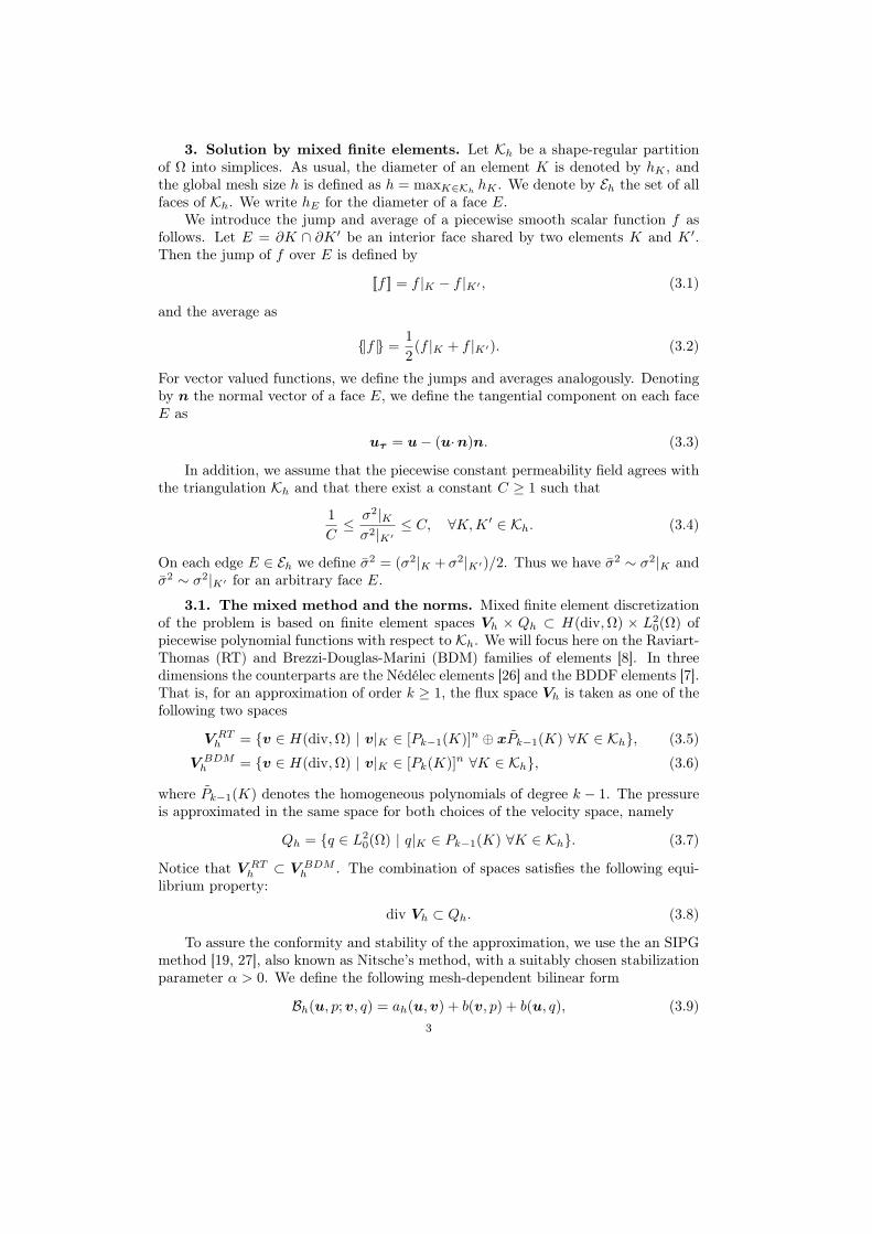
3. Solution by mixed finite elements. Let Kh be a shape-regular partitionof Ω into simplices. As usual, the diameter of an element K is denoted by hK , andthe global mesh size h is defined as h = maxK∈Kh
hK . We denote by Eh the set of allfaces of Kh. We write hE for the diameter of a face E.
We introduce the jump and average of a piecewise smooth scalar function f asfollows. Let E = ∂K ∩ ∂K ′ be an interior face shared by two elements K and K ′.Then the jump of f over E is defined by
[[f ]] = f |K − f |K′ , (3.1)
and the average as
|f | =12
(f |K + f |K′). (3.2)
For vector valued functions, we define the jumps and averages analogously. Denotingby n the normal vector of a face E, we define the tangential component on each faceE as
uτ = u− (u·n)n. (3.3)
In addition, we assume that the piecewise constant permeability field agrees withthe triangulation Kh and that there exist a constant C ≥ 1 such that
1C≤ σ2|Kσ2|K′ ≤ C, ∀K,K ′ ∈ Kh. (3.4)
On each edge E ∈ Eh we define σ2 = (σ2|K + σ2|K′)/2. Thus we have σ2 ∼ σ2|K andσ2 ∼ σ2|K′ for an arbitrary face E.
3.1. The mixed method and the norms. Mixed finite element discretizationof the problem is based on finite element spaces Vh × Qh ⊂ H(div,Ω) × L2
0(Ω) ofpiecewise polynomial functions with respect to Kh. We will focus here on the Raviart-Thomas (RT) and Brezzi-Douglas-Marini (BDM) families of elements [8]. In threedimensions the counterparts are the Nédélec elements [26] and the BDDF elements [7].That is, for an approximation of order k ≥ 1, the flux space Vh is taken as one of thefollowing two spaces
V RTh = v ∈ H(div,Ω) | v|K ∈ [Pk−1(K)]n ⊕ xPk−1(K) ∀K ∈ Kh, (3.5)
V BDMh = v ∈ H(div,Ω) | v|K ∈ [Pk(K)]n ∀K ∈ Kh, (3.6)
where Pk−1(K) denotes the homogeneous polynomials of degree k − 1. The pressureis approximated in the same space for both choices of the velocity space, namely
Qh = q ∈ L20(Ω) | q|K ∈ Pk−1(K) ∀K ∈ Kh. (3.7)
Notice that V RTh ⊂ V BDM
h . The combination of spaces satisfies the following equi-librium property:
div Vh ⊂ Qh. (3.8)
To assure the conformity and stability of the approximation, we use the an SIPGmethod [19, 27], also known as Nitsche’s method, with a suitably chosen stabilizationparameter α > 0. We define the following mesh-dependent bilinear form
Bh(u, p; v, q) = ah(u,v) + b(v, p) + b(u, q), (3.9)3

in which
ah(u,v) = (σ2u,v) + t2
[ ∑K∈Kh
(∇u,∇v)K (3.10)
+∑E∈Eh
αhE〈[[uτ ]], [[vτ ]]〉E − 〈|∂u
∂n|, [[vτ ]]〉E − 〈|∂v
∂n|, [[uτ ]]〉E
].
Then the discrete problem is to find uh ∈ Vh and ph ∈ Qh such that
Bh(uh, ph; v, q) = (f ,v)− (g, q), ∀(v, q) ∈ Vh ×Qh. (3.11)
We introduce the following mesh-dependent norms for the problem. For the ve-locity we use
‖u‖2σ,t,h =∑K∈Kh
σ2‖u‖20,K + t2
[ ∑K∈Kh
‖∇u‖20,K +∑E∈Eh
1hE‖[[uτ ]]‖20,E
], (3.12)
and for the pressure
|||p|||2σ,t,h =∑K∈Kh
h2K
σ2h2K + t2
‖∇p‖20,K +∑E∈Eh
hEσ2h2
E + t2‖[[p]]‖20,E . (3.13)
Note that both of the norms are also parameter dependent. To show continuity, weuse the somewhat stronger norm
‖u‖2σ,t,∗ = ‖u‖2σ,t,h + t2∑E∈Eh
hE‖|∂u
∂n|‖20,E . (3.14)
It is easily shown that the norms (3.12) and (3.14) are equivalent in Vh. We have theresult [30], with CI > 0 .
hE‖∂v
∂n‖20,E ≤ CI‖∇v‖20,K , ∀v ∈ Vh. (3.15)
3.2. A priori analysis. For the proofs of the following results, see [22]. Firstwe note that the method is consistent.
Theorem 3.1. The exact solution (u, p) ∈ V ×Q satisfies
Bh(u, p; v, q) = (f ,v)− (g, q), ∀(v, q) ∈ Vh ×Qh. (3.16)
In addition, the bilinear form ah(· , · ) is coercive in Vh in the mesh-dependentnorm (3.12).
Lemma 3.2. Let CI be the constant from the inequality (3.15). For α > CI/4there exists a positive constant C such that
ah(v,v) ≥ C‖v‖2σ,t,h, ∀v ∈ Vh. (3.17)
With a trivial modification of the proof presented in [22], we have the discreteBrezzi-Babuska stability condition.
4
Lemma 3.3. There exists a positive constant C independent of the parameters tand σ such that
supv∈Vh
b(v, q)‖v‖σ,t,h ≥ C|||q|||σ,t,h, ∀q ∈ Qh. (3.18)
By the above stability results for ah(· , · ) and b(· , · ), the following full stabilityresult holds, see e.g. [8].
Lemma 3.4. There is a positive constant C such that
sup(v,q)∈Vh×Qh
Bh(r, s; v, q)‖v‖σ,t,h + |||q|||σ,t,h ≥ C(‖r‖σ,t,h + |||s|||σ,t,h), ∀(r, s) ∈ Vh ×Qh. (3.19)
In H(div), a special interpolation operator Rh : H(div,Ω)⋂
[Ls(Ω)]n → Vh isrequired, see [8]. We denote by Ph : L2(Ω)→ Qh the L2-projection. The interpolantspossess the following properties:
(div (v −Rhv), q) = 0, ∀q ∈ Qh, (3.20)
(div v, q − Phq) = 0, ∀v ∈ Vh, (3.21)
and
div Rh = Phdiv. (3.22)
By stability and consistency we have the following quasioptimal a priori result shownin [22].
Theorem 3.5. There is a positive constant C such that
‖u− uh‖σ,t,h + |||Php− ph|||σ,t,h ≤ C‖u−Rhu‖σ,t,h. (3.23)
This contains a superconvergence result for |||ph − Php|||σ,t,h, which implies that thepressure solution can be improved by local postprocessing. Given full regularity, weconclude the chapter with the following a priori estimate.
Theorem 3.6. Assuming u ∈ [Hk+1(Ω)]n or u ∈ [Hk(Ω)]n for BDM and RTelements of order k, respectively, we have
‖u− uh‖σ,t,h + |||Php− ph|||σ,t,h ≤C(σh+ t)hk−1‖u‖k, for RT,C(σh+ t)hk‖u‖k+1, for BDM.
(3.24)
3.3. Postprocessing method. We recall the postprocessing method proposedin [22] based on the ideas of [25]. Due to the varying permeability parameter σ, wemodify the method accordingly. We seek the postprocessed pressure in an augmentedspace Q∗h ⊃ Qh, defined as
Q∗h =
q ∈ L2
0(Ω) | q|K ∈ Pk(K) ∀K ∈ Kh, for RT,q ∈ L2
0(Ω) | q|K ∈ Pk+1(K) ∀K ∈ Kh, for BDM.(3.25)
The postprosessing method is: Find p∗h ∈ Q∗h such that
Php∗h = ph (3.26)
(∇p∗h,∇q)K = (t2∆uh − σ2uh + f ,∇q)K , ∀q ∈ (I − Ph)Q∗h|K . (3.27)
5

In [22] the analysis of the postprocessing method is performed by treating it as anintegral part of the problem by embedding it into the bilinear form. Note, that thisis solely for mathematical purposes, in computations the postprocessing is performedafter the solution of the original system elementwise. The modified bilinear form nowreads
B∗h(u, p∗; v, q∗) = Bh(u, p∗; v, q∗)+∑K∈Kh
h2K
σ2h2K + t2
(∇p∗+σ2u−t2∆u,∇(I−Ph)q∗)K .
(3.28)The postprocessed problem is then: Find (uh, p∗h) ∈ Vh×Q∗h such that for every pair(v, q∗) ∈ Vh ×Q∗h it holds
B∗h(uh, p∗h; v, q∗) = Lh(f , Phg; v, q∗), (3.29)
in which
Lh(f , g; v, q∗) = (f ,v)− (g, q∗) +∑K∈Kh
h2K
σ2h2K + t2
(f ,∇(I − Ph)q∗)K . (3.30)
Now using exactly the same arguments as in [22] for the case σ ≡ 1, we can showthat the solutions of the postprocessing procedure and the modified problem (3.29)agree, and we have the following quasioptimal a priori result.
Theorem 3.7. For the postprocessed solution (uh, p∗h) it holds
‖u− uh‖σ,t,h + |||p− p∗h|||σ,t,h ≤ C infq∗∈Q∗h
‖u−Rhu‖σ,t,h + |||p− q∗|||σ,t,h (3.31)
+ (∑K∈Kh
h2K
σ2h2K + t2
‖∇q∗ + σ2Rhu− t2∆Rhu− f‖20,K)1/2.
Assuming full regularity, we have the following optimal a priori result for the post-processed problem.
Theorem 3.8. Let us assume (u, p) ∈ [Hk+1(Ω)]n×Hk+2(Ω) or u ∈ [Hk(Ω)]n××Hk+1(Ω) for BDM and RT elements of order k, respectively. Then we have for thesolution (uh, p∗h) of the postprocessed problem (3.29)
‖u− uh‖σ,t,h + |||p− p∗h|||σ,t,h ≤ C(σh+ t)hk−1‖u‖k +hk+1
σh+ t‖p‖k+1, for RT,
and
‖u− uh‖σ,t,h + |||p− p∗h|||σ,t,h ≤ C(σh+ t)hk‖u‖k+1 +hk+2
σh+ t‖p‖k+2, for BDM.
3.4. A posteriori estimates. In this section we introduce a residual-baseda posteriori estimator for the postprocessed solution. It should be noted that thepostprocessing is vital for a properly functioning estimator. We divide the estimatorinto two distinct parts, one defined over the elements and one over the edges of themesh. The elementwise and edgewise estimators are defined as
η2K =
h2K
σ2h2K + t2
‖ − t2∆uh + σ2uh +∇p∗h − f‖20,K+ (t2 + σ2h2
K)‖g − Phg‖20,K (3.32)
6

η2E =
t2
hE‖[[uh,τ ]]‖20,E +
hEσ2h2
E + t2‖[[t2 ∂uh
∂n]]‖20,E +
hEσ2h2
E + t2‖[[p∗h]]‖20,E . (3.33)
The global estimator is
η =
( ∑K∈Kh
η2K +
∑E∈Eh
η2E
)1/2
. (3.34)
Note that setting t = 0 gives the estimator of [25] for the Darcy problem. In thefollowing, we address the reliability and efficiency of the estimator and show the termsof the estimator to be properly matched to one another. The estimator introducedis both an upper and a lower bound for the actual error as shown by the followingresults, provided that a saturation assumption holds. The arguments presented in [22]hold step-by-step for the estimators (3.32) and (3.33) in conjunction with the scalednorms (3.12) and (3.13).
Theorem 3.9 (Reliability). There exists a constant C > 0 independent of h andthe parameters t and σ such that
‖u− uh‖σ,t,h + |||p− p∗h|||σ,t,h ≤ Cη. (3.35)
Theorem 3.10 (Efficiency). There exists a constant C > 0 independent of h, t,and σ such that
η2 ≤ C‖u− uh‖2σ,t,h + |||p− p∗h|||2σ,t,h (3.36)
+∑K∈Kh
( h2K
σ2h2K + t2
‖f − fh‖20,K + (t2 + σ2h2K)‖g − Phg‖20,K
).
Thus for the displacement uh and the postprocessed pressure p∗h we have byTheorems 3.9 and 3.10 a reliable and efficient indicator for an elementwise constantpermeability parameter σ and all values of the effective viscosity parameter t. Inaddition, we have the localized lower bound
η2K + η2
E ≤ C‖u− uh‖2σ,t,h,ωK
+ |||p− p∗h|||2σ,t,h,ωK(3.37)
+∑K∈ωK
( h2K
σ2h2K + t2
‖f − fh‖20,K + (t2 + σ2h2K)‖g − Phg‖20,K
),
in which ωK ⊂ Ω is the patch of elements surrounding an element K, and the sub-scripted norms above are evaluated only over the elements in ωK . Thus we have astrong indication of the applicability of the estimator to adaptive refinement.
4. Hybridization. A well-known method for dealing with the indefinite systemresulting in from the Darcy equation is the hybridization technique introduced in [5,8]. The idea is to enforce the tangential continuity via Lagrange multipliers chosensuitably and relaxing the continuity requirement on the finite element space. Thus,we drop the normal continuity requirement in the spaces V BDM
h and V RTh and denote
these discontinuous counterparts by Vh. In addition, we introduce the correspondingmultiplier spaces
ΛBDMh = λ ∈ [L2(Eh)]n−1 | λ ∈ Pk(E), E ∈ Eh, λ|E = 0, E ⊂ ∂Ω, (4.1)
ΛRTh = λ ∈ [L2(Eh)]n−1 | λ ∈ Pk−1(E), E ∈ Eh, λ|E = 0, E ⊂ ∂Ω, (4.2)
7
in which Eh denotes the collection of all faces of the mesh. It can be easily shown,that the normal continuity of a discrete flux uh ∈ Vh is equivalent to the requirement∑
K∈Kh
〈uh·n, µ〉∂K = 0, ∀µ ∈ Λh. (4.3)
Accordingly, the original finite element problem (3.11) can be hybridized in the fol-lowing form: Find (uh, ph, λh) ∈ Vh ×Qh × Λh such that
Bh(uh, ph; v, q) +∑K∈Kh
〈v·n, λh〉∂K = (f ,v) + (g, q), (4.4)
∑K∈Kh
〈uh·n, µ〉∂K = 0 (4.5)
for all (v, q, µ) ∈ Vh ×Qh × Λh. Due to (4.3), the solution (uh, ph) of the hybridizedsystem coincides with that of the original system. Thus, we need not modify thepostprocessing procedure even if we drop the continuity requirement from the velocityspace.
4.1. Hybridization of the Nitsche term. However, now the matrix blockcorresponding to the bilinear form Bh(uh, ph; v, q) is a block diagonal system only forthe special case t = 0, and for a non-zero effective viscosity we cannot eliminate thevariables locally. To alleviate this problem we introduce a second hybrid variable forthe Nitsche term of the velocity, see e.g. [10]. Recall, that the velocity-velocity termof the bilinear form Bh(uh, ph; v, q) is
ah(u,v) = (σ2u,v) + t2
[ ∑K∈Kh
(∇u,∇v)K (4.6)
+∑E∈Eh
αhE〈[[uτ ]], [[vτ ]]〉E − 〈|∂u
∂n|, [[vτ ]]〉E − 〈|∂v
∂n|, [[uτ ]]〉E
].
To this end, we follow [12], and formally introduce the mean value of uτ as a newvariable, m = 1
2 (u1,τ + u2,τ ). Thus we can write the tangential jump as
[[uτ ]] = 2(u1,τ −m) = −2(u2,τ −m). (4.7)
Now using the new hybrid variables the bilinear form ah(u,v) can be rewritten as
ah(u,m; v, r) = (σ2u,v) + t2∑K∈Kh
(∇u,∇v)K +2αhE〈uτ −m,vτ − r〉∂K
− 〈∂u
∂n,vτ − r〉∂K − 〈∂v
∂n,uτ −m〉∂K.
Here, the hybrid variable m belongs to a spaceMh ⊂ [L2(Eh)]n, the choice of whichwill be discussed subsequently. In addition, we introduce a slightly modified versionof the norm (3.12) to encompass both the velocity and the hybrid variable:
‖(u,m)‖2σ,t,h =∑K∈Kh
σ2‖u‖20,K + t2
[ ∑K∈Kh
‖∇u‖20,K +∑E∈Eh
1hE‖uτ −m‖20,E
].
(4.8)8

Since for the exact solution the jumps disappear, the bilinear form is consistent.Using exactly the same arguments as those presented in [12] for (3.17), we have
Lemma 4.1. The hybridized bilinear form ah(· , · ; · , · ) is coercive in the discretespaces Vh ×Mh, that is there exists a positive constant C such that
ah(v,m; v,m) ≥ C‖(v,m)‖2σ,t,h, ∀(v,m) ∈ Vh ×Mh. (4.9)
Note, that the stability holds for any choice of the space Mh. For complicatedproblems, this gives great flexibility. Thus, due to consistency and stability, we getoptimal convergence rate as long as the spaceMh is rich enough. Here we choose
Mh = m ∈ [L2(Eh)]n | Q(E)m|E ∈ [Pk(E)]n−1, ∀E ∈ Eh, (4.10)
in which Q(E) is the coordinate transformation matrix from the global n-dimensionalcoordinate system to the local (n− 1)-dimensional coordinate system on the face E.Let Ph : [L2(E)]n−1 → Mh be the L2 projection on the faces. We then get thefollowing interpolation estimate.
Lemma 4.2. Let u be such that u|K ∈ [Hs+1(K)]n for 12 < s ≤ k. Then it holds
‖(u−Rhu,uτ − Phuτ )‖σ,t,h ≤ C(σh+ t)hs‖u‖s+1. (4.11)
Proof. We proceed by direct computation. Scaling and the Bramble-Hilbertlemma [6] yield
‖(u−Rhu,uτ−Phuτ )‖2σ,t,h ≤∑K∈Kh
σ2‖u−Rhu‖20,K+t2[ ∑K∈Kh
‖∇(u−Rhu)‖20,K
+∑E∈Eh
(1hE‖(u−Rhu)τ‖20,E +
1hE‖(uτ − Phuτ )‖20,E
)]
≤ C(σ2h2s+2‖u‖2s+1 + t2
∑K∈Kh
h2sK ‖u‖2s+1,K + h2s
K ‖uτ‖2s+1/2,K).
The result is immediate after taking the square root.Combining the interpolation results with the consistency and ellipticity properties
yields an optimal convergence rate for the velocity.Theorem 4.3. Assuming sufficient regularity, for the finite element solution
(uh,mh) of the hybridized system it holds
‖(u− uh,uτ −mh))‖σ,t,h ≤ C(σh+ t)hs‖u‖s+1. (4.12)
Thus the hybridization preserves the convergence rates of Theorem 3.8.The residual a posteriori estimator of Section 3.4 can be modified to handle the
hybrid variable by changing the edgewise estimator (3.33) to
η2E =
t2
hE‖uh,τ −mh‖20,E +
hEσ2h2
E + t2‖[[t2 ∂uh
∂n]]‖20,E +
hEσ2h2
E + t2‖[[p∗h]]‖20,E . (4.13)
Following the lines of the proof in [22] it is easy to prove that also the modified esti-mator is both sharp and reliable. This will be demonstrated in numerical experimentsin Section 5.
9
4.2. Implementation and local condensation. In practice, it is beneficialto choose the hybrid variable m slightly differently, namely as the weighted averagem = t
2 (u1,τ + u2,τ ). Now the hybridized bilinear form can be written as
ah(u,m; v, r) = (σ2u,v) +∑K∈Kh
2αhE〈m, r〉∂K
+ t∑K∈Kh
〈∂u
∂n, r〉∂K + 〈∂v
∂n,m〉∂K − 2α
hE〈uτ , r〉∂K − 2α
hE〈vτ ,m〉∂K
+ t2∑K∈Kh
(∇u,∇v)K +2αhE〈uτ ,vτ 〉∂K − 〈∂u
∂n,vτ 〉∂K − 〈∂u
∂n,uτ 〉∂K.
Note, that now we get a t-independent part for the hybrid variable and the systemremains solvable even in the limit t→ 0. It is clear that all of the results in Section 4.1hold also for the scaled hybrid variable.
The main motivation for the hybridization procedure is to break all connectionsin the original saddlepoint system to allow for local elimination of the velocity andpressure variables at the element level. After hydridization the matrix system getsthe following form where A is the matrix corresponding to the bilinear form ah(· , · ),B to b(· , · ), whilst C and D represent the connecting blocks for the hybrid variablesfor normal continuity and the Nitsche terms, respectively. M is the mass matrix forthe Nitsche hybrid variable.
A BT CT DT
B 0 0 0C 0 0 0D 0 0 M
. (4.14)
Since A and B are now block diagonal matrices, they can be inverted on theelement level and we get the following symmetric and positive definite system for thehybrid variables. We denote the by H the following matrix that can be computedelementwise.
H := A−1BT (BA−1BT )−1BA−1 −A−1. (4.15)
The matrix H is positive definite and symmetric. Eliminating the velocity and pres-sure from the system matrix (4.14) yields the following system matrix for the hybridvariables (λ,m) corresponding to the normal continuity and tangential jumps, respec-tively. (
CHCT CHDT
DHCT DHDT +M
). (4.16)
Evidently the resulting system is symmetric and positive definite. Note, that whilstthe connecting block D will vanish as t→ 0, the M block does not depend on t, thusthe whole system remains invertible even in the limit.
4.3. Application to domain decomposition. The hybridized formulation iswell-suited to solving large problems with the domain decomposition method. The
10
hybrid variables readily form a discretization for the skeleton of the domain decom-position method for any choice of non-overlapping blocks. The local problems are ofthe Dirichlet type, and the domain decomposition method can be implemented easilyusing local solvers on the subdomains.
Furthermore, only the skeleton of the domain decomposition mesh can be hy-bridized using conventional H(div)-elements for the saddle point system in the sub-domains. We also have great flexibility in the choice of the hybridized variables, thusallowing one to use a lower number of degrees of freedom on the skeleton when com-putational resources are limited or alternatively construct a coarser approximationfor use as a preconditioner. Most importantly, the mass conservation property is re-tained over the subdomain boundaries, thus making the method a viable alternativefor multiphase flow computations.
5. Numerical tests. In this section, we shall numerically demonstrate the per-formance of the method. In all of the convergence tests we are mainly interested inthe effect of the ratio between the Stokes and Darcy terms −t2∆u and σ2u. Thus forthe convergence tests we reduce the problem to a one-parameter family of problemsby choosing σ = 1 on the whole of the domain Ω. This allows us to visualize differ-ent behavior of the numerical method in the Stokes and Darcy regimes for varyingparameter values.
First, we test the optimal convergence properties of the method along with theperformance of the a posteriori estimator in two cases with different regularity prop-erties. The proposed method is also compared with the Stokes-type approach usingthe MINI element. We proceed to demonstrate the effect and the importance of thepostprocessing procedure. Next, the convergence of the hybridized method is studiedin the framework of domain decomposition methods. Our fourth test is the classi-cal Poisseuille flow, demonstrating the performance of Nitsche’s method in assign-ing the boundary conditions and the applicability of the error indicator to adaptivemesh refinement. We end the section with a realistic example employing permeabil-ity data from the SPE10 dataset. In all of the test cases the ratio h/t is the ratio1/(t√N), in which N is the number of degrees of freedom. For a uniform mesh we
have h/t ≈ 1/(t√N). Note, that this holds only in the two-dimensional case consid-
ered in the computations. The data approximation term in the a posteriori estimatoris neglected in the computations.
5.1. Convergence tests. For the purpose of testing the convergence rate, wepick a pressure p such that ∇p is a harmonic function. Thus, u = ∇p is a solution ofthe problem for every t ≥ 0. In polar coordinates (r,Θ) the pressure is chosen as
p(r,Θ) = rβ sin(βΘ) + C. (5.1)
The constant C is chosen such that the pressure will have a zero mean value. Moreover,we have p ∈ H1+β(Ω), and subsequently u ∈ [Hβ(Ω)]n, see [14]. In the following,we have tested the convergence with a wide range of different parameter values, andthe results are plotted with respect to the ratio of the viscosity parameter t to themesh size h. Our aim is to demonstrate numerically, that the change in the natureof the problem indeed occurs at t = h, and that the convergence rates are optimal inboth of the limiting cases. First we choose β = 3.1 to test the convergence rates ina smooth situation. With the first-order BDM element we are expecting h2 convergein the Darcy end of the parameter range and h in the Stokes limit.
As is visible from the results in Figures 1 and 2, the behaviour of the problemchanges numerically when t = h. Thus, even though in practical applications almost
11

always t > 0, numerically the problem behaves like the Darcy problem when t < h.As can be seen from Figure 2, the converge rates follow quite closely those given bythe theory. Furthermore, both the actual error and the a posteriori indicator behavein a similar manner. Notice, that the convergence rate exhibits a slight dip at thepoint in which the nature of the problem changes. This is a result of the dominatingerror component changing from pressure to velocity error as we pass into the Stokesregime.
To show the applicability of the a posteriori indicator to mesh refinement, weconsider the more irregular case β = 1.52. Our refinement strategy consists of refin-ing those elements in which the error exceeds 50 percent of the average value. Thetreshold is halved until at least five percent of the elements have been refined. Theedge estimators are shared evenly between the neighbouring elements. Figure 6 shows,that the converge is considerably faster with adaptive refinement, as opposed to uni-form refinement in Figure 4. Furthermore, adaptive refinement seems to alleviate theproblem of convergence rate drop at the numerical turning point t = h. Clearly theseresults indicate that the a posteriori indicator proposed gives reasonable local boundsand can thus be used in adaptive mesh refinement.
5.2. Comparison with the MINI element. A common choice for solving theStokes problem is the classical MINI element [4]. This element has been applied tothe Brinkman problem and thoroughly analyzed both theoretically and numericallyin [19, 16]. We use the same test case as above with the regularity parameter set toβ = 3.1. Notice, that the mesh-dependent norms (3.12) and (3.13) reduce to the onespresented in [19] when a continuous velocity-pressure pair is inserted. Thus we canuse the same mesh-dependent norm for computing the error for both of the elementsand the results are comparable with one another.
As can be seen from the results in Figure 8, the convergence rate for the MINIelement is as expected of the order h throughout the parameter regime. For the BDM1element, on the other hand, we get h2 convergence in the Darcy regime, and after aslight dip at the turnaround point convergence relative to h. Turning our attention toFigure 7 reveals that the behaviour of the absolute value of the relative error differsvastly for the two elements. Clearly, the BDM element outperforms the MINI elementin the Darcy regime by several decades of magnitude, whereas in the Stokes regimethe performance of the MINI element is superior. This implicates that it is impossibleto clearly tell which element is superior for the Brinkman flow. However, usually real-life reservoirs consist mostly of porous stone with scattered vugs and cracks. Thusthe volume of the Stokes-type regime is often small compared to the Darcy regime,implying that the good performance of the BDM element in its natural operationconditions might offer significant performance increase for the overall simulation. Inproblems with a greater fraction of void space, such as filters with large free-flowareas separated by permeable thin layers, the Stokes-based elements might be a morenatural choice.
5.3. Postprocessing. In this section, we show the necessity of the postprocess-ing by comparing the behaviour of both the exact error and the a posteriori estimatorfor the original and the postprocessed pressure. We shall use the same test case as inthe previous sections. First we choose β = 3.1 for testing the effect of the postpro-cessign on the convergence. On the second run we choose β = 1.52 and use the samemesh refinement strategy as before to show the necessity of the post-processing forthe usefulness of the error estimator.
From the results of Figure 9, it is immediately evident that in the case of a small12
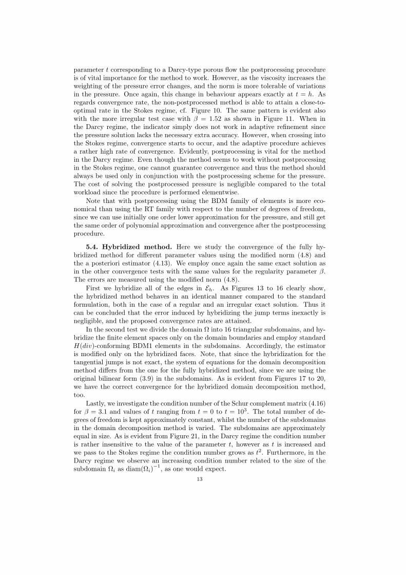
parameter t corresponding to a Darcy-type porous flow the postprocessing procedureis of vital importance for the method to work. However, as the viscosity increases theweighting of the pressure error changes, and the norm is more tolerable of variationsin the pressure. Once again, this change in behaviour appears exactly at t = h. Asregards convergence rate, the non-postprocessed method is able to attain a close-to-optimal rate in the Stokes regime, cf. Figure 10. The same pattern is evident alsowith the more irregular test case with β = 1.52 as shown in Figure 11. When inthe Darcy regime, the indicator simply does not work in adaptive refinement sincethe pressure solution lacks the necessary extra accuracy. However, when crossing intothe Stokes regime, convergence starts to occur, and the adaptive procedure achievesa rather high rate of convergence. Evidently, postprocessing is vital for the methodin the Darcy regime. Even though the method seems to work without postprocessingin the Stokes regime, one cannot guarantee convergence and thus the method shouldalways be used only in conjunction with the postprocessing scheme for the pressure.The cost of solving the postprocessed pressure is negligible compared to the totalworkload since the procedure is performed elementwise.
Note that with postprocessing using the BDM family of elements is more eco-nomical than using the RT family with respect to the number of degrees of freedom,since we can use initially one order lower approximation for the pressure, and still getthe same order of polynomial approximation and convergence after the postprocessingprocedure.
5.4. Hybridized method. Here we study the convergence of the fully hy-bridized method for different parameter values using the modified norm (4.8) andthe a posteriori estimator (4.13). We employ once again the same exact solution asin the other convergence tests with the same values for the regularity parameter β.The errors are measured using the modified norm (4.8).
First we hybridize all of the edges in Eh. As Figures 13 to 16 clearly show,the hybridized method behaves in an identical manner compared to the standardformulation, both in the case of a regular and an irregular exact solution. Thus itcan be concluded that the error induced by hybridizing the jump terms inexactly isnegligible, and the proposed convergence rates are attained.
In the second test we divide the domain Ω into 16 triangular subdomains, and hy-bridize the finite element spaces only on the domain boundaries and employ standardH(div)-conforming BDM1 elements in the subdomains. Accordingly, the estimatoris modified only on the hybridized faces. Note, that since the hybridization for thetangential jumps is not exact, the system of equations for the domain decompositionmethod differs from the one for the fully hybridized method, since we are using theoriginal bilinear form (3.9) in the subdomains. As is evident from Figures 17 to 20,we have the correct convergence for the hybridized domain decomposition method,too.
Lastly, we investigate the condition number of the Schur complement matrix (4.16)for β = 3.1 and values of t ranging from t = 0 to t = 103. The total number of de-grees of freedom is kept approximately constant, whilst the number of the subdomainsin the domain decomposition method is varied. The subdomains are approximatelyequal in size. As is evident from Figure 21, in the Darcy regime the condition numberis rather insensitive to the value of the parameter t, however as t is increased andwe pass to the Stokes regime the condition number grows as t2. Furthermore, in theDarcy regime we observe an increasing condition number related to the size of thesubdomain Ωi as diam(Ωi)
−1, as one would expect.13

5.5. Poisseuille flow. The Poisseuille flow is a classical test case for which theexact solution is known. The setup represents a viscous flow in a long, narrow channel.The flow is driven by a linear pressure drop with no-slip boundary conditions for t > 0.For the Darcy case t = 0, only the normal component of the velocity vanishes on theboundary. We will test the convergence with Nitsche’s method for the tangentialboundary condition with adaptive mesh refinement. Denote by Eh,uτ the collection ofedges residing on the part of the boundary Γuτ ⊂ ∂Ω on which we set the tangentialvelocity. To set the tangential velocity we then add the term
t2∑
E∈Eh,uτ
αhE〈uτ ,vτ 〉E − 〈∂u
∂n,vτ 〉E − 〈∂v
∂n,uτ 〉E (5.2)
to the bilinear form ah(· , · ). The loading is augmented by the term
t2∑
E∈Eh,uτ
αhE〈uD,τ ,vτ 〉E − 〈∂v
∂n,uD,τ 〉E. (5.3)
in which uD denotes the velocity boundary condition. Finally, the error estima-tor (3.33) is modified by adding the corresponding boundary face terms to the esti-mator.
In the unit square we take the pressure to be p = −x + 12 . Then zero boundary
conditions for the velocity give the exact solution u = (u, 0), with the x-directionalvelocity given by
u =
(1 + e1/t − e(1−y)/t − ey/t)/(1 + e1/t), t > 01, t = 0.
(5.4)
As Figures 22 through 26 demonstrate, the adaptive process is able to catchthe boundary layer effectively, leading to nearly identical converge rates for differentparameter values as indicated by Figure 27. Note, that as the mesh is refined on theedges, the problem changes numerically to a Stokes-type problem near the boundarysince the mesh size h drops locally below the parameter t.
5.6. Example with realistic material parameters. In this final section weconsider the Society of Petroleum Engineers test case SPE10 [9] with realistic porosityand permeability data for a heteregeneous oil reservoir. Following [28], we make thecommon choice µ = µ. We consider a single layer flow as a two-dimensional flowproblem. For the outflow quantities to have meaningful units, we assume a thicknessof 2 ft for the layer. The dimensions of the problem are 2200 × 1200 ft, the fluid ischosen as e.g. water with a viscosity of 1 cP. The flow is driven by a pressure onthe left-hand side of the domain. The top and bottom boundaries have a no-flowboundary condition. To demonstrate the effect of the Brinkman term to the flow, wemodify the permeability data by adding a rectangular streak of very high permeabilitywith the dimensions 1100× 20 ft in the middle of the domain. The advantage of theBrinkman model is the ability to model cracks or vugs by simply assigning a veryhigh (or infinite) permeability to these parts of the domain.
In the numerical tests the performance of the a posteriori estimator for adaptiverefinement with extremely heterogenous data with vast differences in magnitude isstudied. We start all of the computations from a coarse triangulation of the domainwith 328 triangles and 1352 total degrees of freedom. This results in an initial element
14
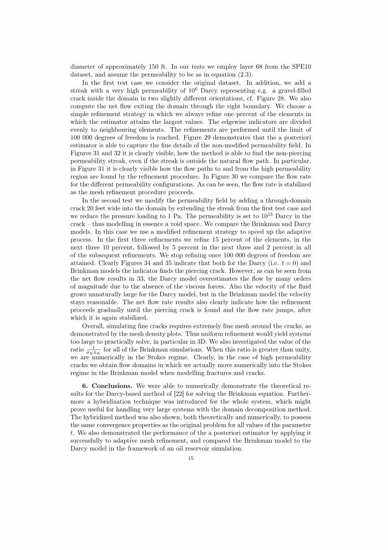
diameter of approximately 150 ft. In our tests we employ layer 68 from the SPE10dataset, and assume the permeability to be as in equation (2.3).
In the first test case we consider the original dataset. In addition, we add astreak with a very high permeability of 106 Darcy representing e.g. a gravel-filledcrack inside the domain in two slightly different orientations, cf. Figure 28. We alsocompute the net flow exiting the domain through the right boundary. We choose asimple refinement strategy in which we always refine one percent of the elements inwhich the estimator attains the largest values. The edgewise indicators are dividedevenly to neighbouring elements. The refinements are performed until the limit of100 000 degrees of freedom is reached. Figure 29 demonstrates that the a posterioriestimator is able to capture the fine details of the non-modified permeability field. InFigures 31 and 32 it is clearly visible, how the method is able to find the non-piercingpermeability streak, even if the streak is outside the natural flow path. In particular,in Figure 31 it is clearly visible how the flow paths to and from the high permeabilityregion are found by the refinement procedure. In Figure 30 we compare the flow ratefor the different permeability configurations. As can be seen, the flow rate is stabilizedas the mesh refinement procedure proceeds.
In the second test we modify the permeability field by adding a through-domaincrack 20 feet wide into the domain by extending the streak from the first test case andwe reduce the pressure loading to 1 Pa. The permeability is set to 1015 Darcy in thecrack – thus modelling in essence a void space. We compare the Brinkman and Darcymodels. In this case we use a modified refinement strategy to speed up the adaptiveprocess. In the first three refinements we refine 15 percent of the elements, in thenext three 10 percent, followed by 5 percent in the next three and 2 percent in allof the subsequent refinements. We stop refining once 100 000 degrees of freedom areattained. Clearly Figures 34 and 35 indicate that both for the Darcy (i.e. t = 0) andBrinkman models the indicator finds the piercing crack. However, as can be seen fromthe net flow results in 33, the Darcy model overestimates the flow by many ordersof magnitude due to the absence of the viscous forces. Also the velocity of the fluidgrows unnaturally large for the Darcy model, but in the Brinkman model the velocitystays reasonable. The net flow rate results also clearly indicate how the refinementproceeds gradually until the piercing crack is found and the flow rate jumps, afterwhich it is again stabilized.
Overall, simulating fine cracks requires extremely fine mesh around the cracks, asdemonstrated by the mesh density plots. Thus uniform refinement would yield systemstoo large to practically solve, in particular in 3D. We also investigated the value of theratio t
σKhKfor all of the Brinkman simulations. When this ratio is greater than unity,
we are numerically in the Stokes regime. Clearly, in the case of high permeabilitycracks we obtain flow domains in which we actually move numerically into the Stokesregime in the Brinkman model when modelling fractures and cracks.
6. Conclusions. We were able to numerically demonstrate the theoretical re-sults for the Darcy-based method of [22] for solving the Brinkman equation. Further-more a hybridization technique was introduced for the whole system, which mightprove useful for handling very large systems with the domain decomposition method.The hybridized method was also shown, both theoretically and numerically, to possessthe same convergence properties as the original problem for all values of the parametert. We also demonstrated the performance of the a posteriori estimator by applying itsuccessfully to adaptive mesh refinement, and compared the Brinkman model to theDarcy model in the framework of an oil reservoir simulation.
15

Acknowledgement. This work has been supported by the Finnish ResearchProgramme on Nuclear Waste Management (KYT) and the Finnish National Gradu-ate School in Engineering Mechanics. In addition, the first author has been supportedby the Finnish Cultural Foundation.
16
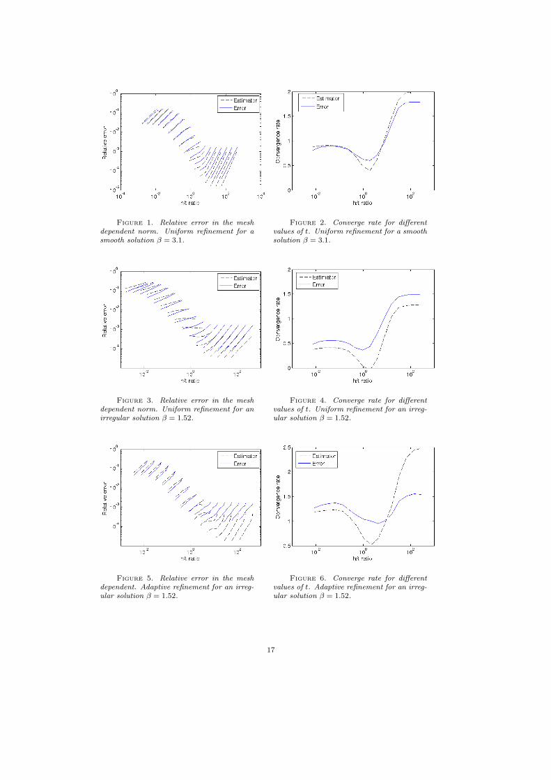
Figure 1. Relative error in the meshdependent norm. Uniform refinement for asmooth solution β = 3.1.
Figure 2. Converge rate for differentvalues of t. Uniform refinement for a smoothsolution β = 3.1.
Figure 3. Relative error in the meshdependent norm. Uniform refinement for anirregular solution β = 1.52.
Figure 4. Converge rate for differentvalues of t. Uniform refinement for an irreg-ular solution β = 1.52.
Figure 5. Relative error in the meshdependent. Adaptive refinement for an irreg-ular solution β = 1.52.
Figure 6. Converge rate for differentvalues of t. Adaptive refinement for an irreg-ular solution β = 1.52.
17
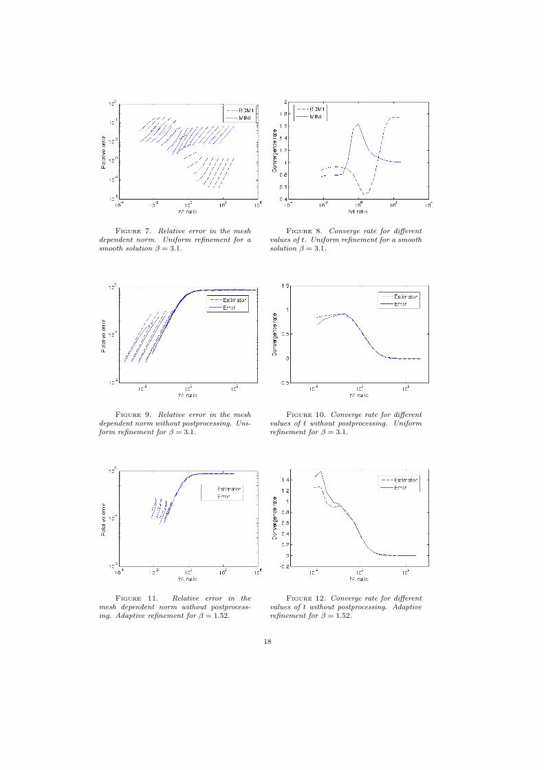
Figure 7. Relative error in the meshdependent norm. Uniform refinement for asmooth solution β = 3.1.
Figure 8. Converge rate for differentvalues of t. Uniform refinement for a smoothsolution β = 3.1.
Figure 9. Relative error in the meshdependent norm without postprocessing. Uni-form refinement for β = 3.1.
Figure 10. Converge rate for differentvalues of t without postprocessing. Uniformrefinement for β = 3.1.
Figure 11. Relative error in themesh dependent norm without postprocess-ing. Adaptive refinement for β = 1.52.
Figure 12. Converge rate for differentvalues of t without postprocessing. Adaptiverefinement for β = 1.52.
18
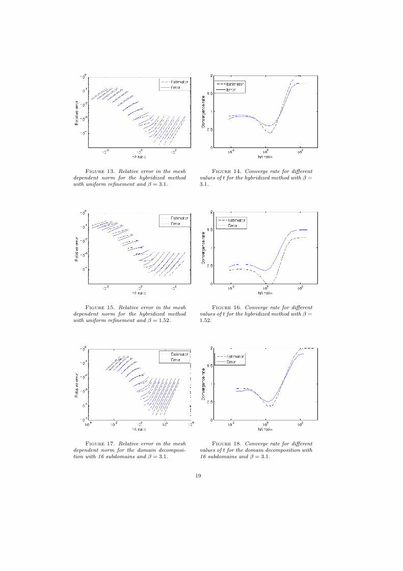
Figure 13. Relative error in the meshdependent norm for the hybridized methodwith uniform refinement and β = 3.1.
Figure 14. Converge rate for differentvalues of t for the hybridized method with β =3.1.
Figure 15. Relative error in the meshdependent norm for the hybridized methodwith uniform refinement and β = 1.52.
Figure 16. Converge rate for differentvalues of t for the hybridized method with β =1.52.
Figure 17. Relative error in the meshdependent norm for the domain decomposi-tion with 16 subdomains and β = 3.1.
Figure 18. Converge rate for differentvalues of t for the domain decomposition with16 subdomains and β = 3.1.
19

Figure 19. Relative error in the meshdependent norm for the domain decomposi-tion with 16 subdomains and β = 1.52.
Figure 20. Converge rate for differentvalues of t for the domain decomposition with16 subdomains and β = 1.52.
Figure 21. Condition number for several subdomain divisions for different values of t.
20

Figure 22. Final mesh after adaptiverefinement, t = 0.5
Figure 23. Final mesh after adaptiverefinement, t = 0.2
Figure 24. Final mesh after adaptiverefinement, t = 0.1
Figure 25. Final mesh after adaptiverefinement, t = 0.05
Figure 26. Final mesh after adaptiverefinement, t = 0.005
Figure 27. Convergence rates of theadaptive solution for different values of t.
21
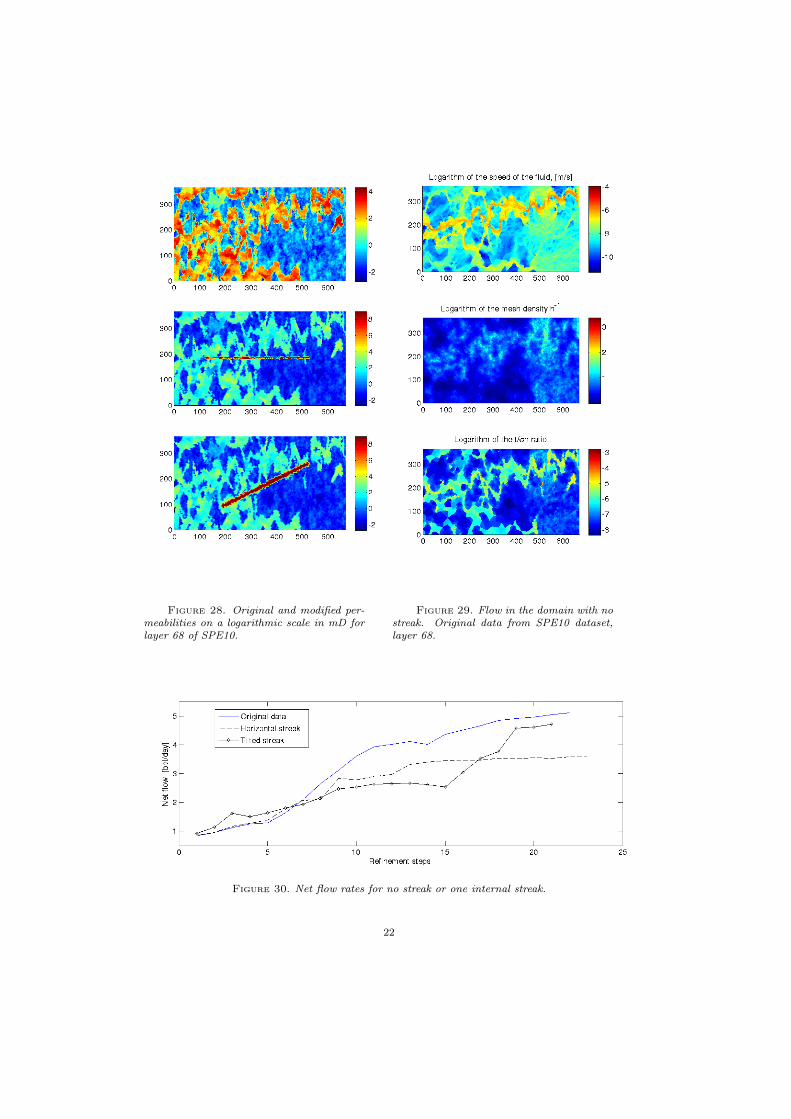
Figure 28. Original and modified per-meabilities on a logarithmic scale in mD forlayer 68 of SPE10.
Figure 29. Flow in the domain with nostreak. Original data from SPE10 dataset,layer 68.
Figure 30. Net flow rates for no streak or one internal streak.
22
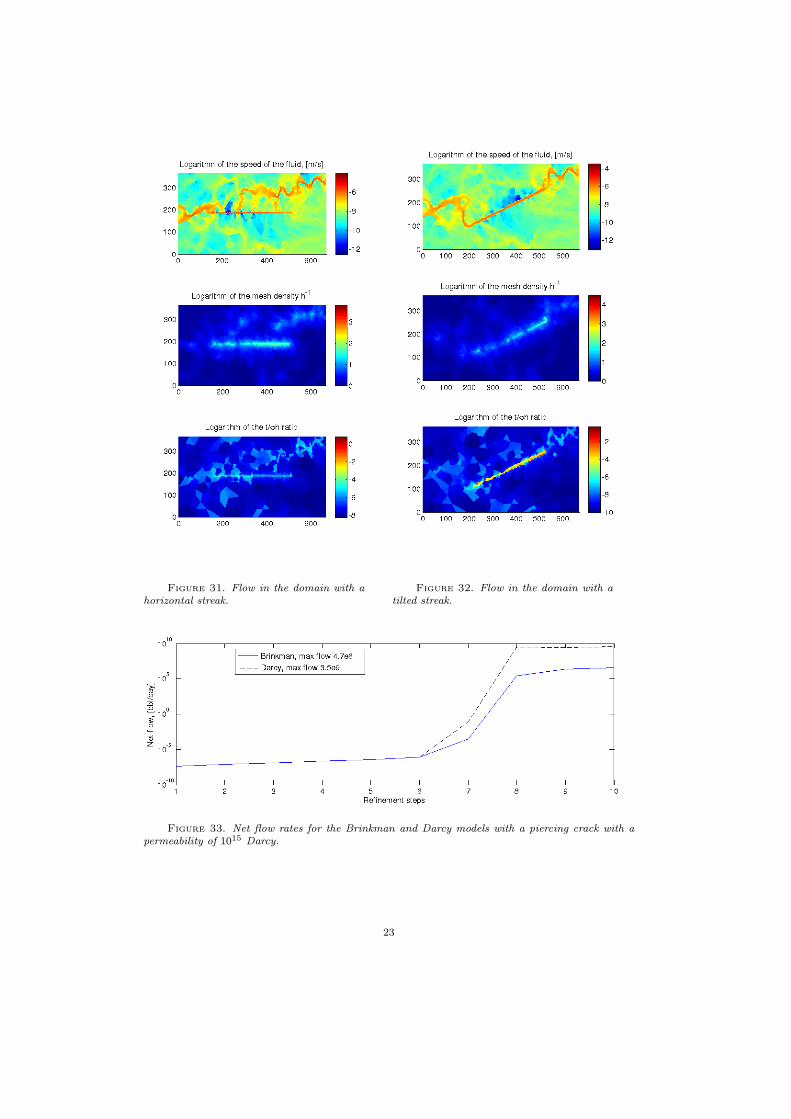
Figure 31. Flow in the domain with ahorizontal streak.
Figure 32. Flow in the domain with atilted streak.
Figure 33. Net flow rates for the Brinkman and Darcy models with a piercing crack with apermeability of 1015 Darcy.
23

Figure 34. Flow in the domain with apiercing crack, Brinkman model.
Figure 35. Flow in the domain with apiercing crack, Darcy model.
24
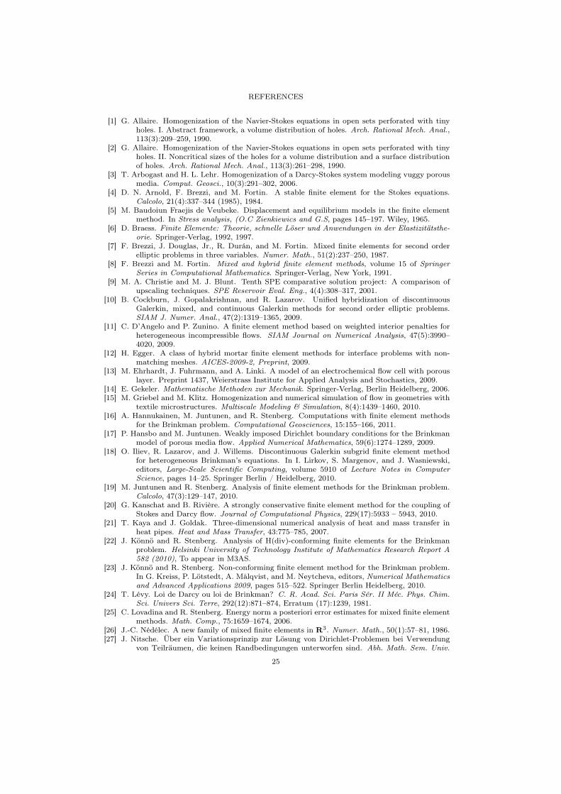
REFERENCES
[1] G. Allaire. Homogenization of the Navier-Stokes equations in open sets perforated with tinyholes. I. Abstract framework, a volume distribution of holes. Arch. Rational Mech. Anal.,113(3):209–259, 1990.
[2] G. Allaire. Homogenization of the Navier-Stokes equations in open sets perforated with tinyholes. II. Noncritical sizes of the holes for a volume distribution and a surface distributionof holes. Arch. Rational Mech. Anal., 113(3):261–298, 1990.
[3] T. Arbogast and H. L. Lehr. Homogenization of a Darcy-Stokes system modeling vuggy porousmedia. Comput. Geosci., 10(3):291–302, 2006.
[4] D. N. Arnold, F. Brezzi, and M. Fortin. A stable finite element for the Stokes equations.Calcolo, 21(4):337–344 (1985), 1984.
[5] M. Baudoiun Fraejis de Veubeke. Displacement and equilibrium models in the finite elementmethod. In Stress analysis, (O.C Zienkiewics and G.S, pages 145–197. Wiley, 1965.
[6] D. Braess. Finite Elemente: Theorie, schnelle Löser und Anwendungen in der Elastizitätsthe-orie. Springer-Verlag, 1992, 1997.
[7] F. Brezzi, J. Douglas, Jr., R. Durán, and M. Fortin. Mixed finite elements for second orderelliptic problems in three variables. Numer. Math., 51(2):237–250, 1987.
[8] F. Brezzi and M. Fortin. Mixed and hybrid finite element methods, volume 15 of SpringerSeries in Computational Mathematics. Springer-Verlag, New York, 1991.
[9] M. A. Christie and M. J. Blunt. Tenth SPE comparative solution project: A comparison ofupscaling techniques. SPE Reservoir Eval. Eng., 4(4):308–317, 2001.
[10] B. Cockburn, J. Gopalakrishnan, and R. Lazarov. Unified hybridization of discontinuousGalerkin, mixed, and continuous Galerkin methods for second order elliptic problems.SIAM J. Numer. Anal., 47(2):1319–1365, 2009.
[11] C. D’Angelo and P. Zunino. A finite element method based on weighted interior penalties forheterogeneous incompressible flows. SIAM Journal on Numerical Analysis, 47(5):3990–4020, 2009.
[12] H. Egger. A class of hybrid mortar finite element methods for interface problems with non-matching meshes. AICES-2009-2, Preprint, 2009.
[13] M. Ehrhardt, J. Fuhrmann, and A. Linki. A model of an electrochemical flow cell with porouslayer. Preprint 1437, Weierstrass Institute for Applied Analysis and Stochastics, 2009.
[14] E. Gekeler. Mathematische Methoden zur Mechanik. Springer-Verlag, Berlin Heidelberg, 2006.[15] M. Griebel and M. Klitz. Homogenization and numerical simulation of flow in geometries with
textile microstructures. Multiscale Modeling & Simulation, 8(4):1439–1460, 2010.[16] A. Hannukainen, M. Juntunen, and R. Stenberg. Computations with finite element methods
for the Brinkman problem. Computational Geosciences, 15:155–166, 2011.[17] P. Hansbo and M. Juntunen. Weakly imposed Dirichlet boundary conditions for the Brinkman
model of porous media flow. Applied Numerical Mathematics, 59(6):1274–1289, 2009.[18] O. Iliev, R. Lazarov, and J. Willems. Discontinuous Galerkin subgrid finite element method
for heterogeneous Brinkman’s equations. In I. Lirkov, S. Margenov, and J. Wasniewski,editors, Large-Scale Scientific Computing, volume 5910 of Lecture Notes in ComputerScience, pages 14–25. Springer Berlin / Heidelberg, 2010.
[19] M. Juntunen and R. Stenberg. Analysis of finite element methods for the Brinkman problem.Calcolo, 47(3):129–147, 2010.
[20] G. Kanschat and B. Rivière. A strongly conservative finite element method for the coupling ofStokes and Darcy flow. Journal of Computational Physics, 229(17):5933 – 5943, 2010.
[21] T. Kaya and J. Goldak. Three-dimensional numerical analysis of heat and mass transfer inheat pipes. Heat and Mass Transfer, 43:775–785, 2007.
[22] J. Könnö and R. Stenberg. Analysis of H(div)-conforming finite elements for the Brinkmanproblem. Helsinki University of Technology Institute of Mathematics Research Report A582 (2010), To appear in M3AS.
[23] J. Könnö and R. Stenberg. Non-conforming finite element method for the Brinkman problem.In G. Kreiss, P. Lötstedt, A. Målqvist, and M. Neytcheva, editors, Numerical Mathematicsand Advanced Applications 2009, pages 515–522. Springer Berlin Heidelberg, 2010.
[24] T. Lévy. Loi de Darcy ou loi de Brinkman? C. R. Acad. Sci. Paris Sér. II Méc. Phys. Chim.Sci. Univers Sci. Terre, 292(12):871–874, Erratum (17):1239, 1981.
[25] C. Lovadina and R. Stenberg. Energy norm a posteriori error estimates for mixed finite elementmethods. Math. Comp., 75:1659–1674, 2006.
[26] J.-C. Nédélec. A new family of mixed finite elements in R3. Numer. Math., 50(1):57–81, 1986.[27] J. Nitsche. Über ein Variationsprinzip zur Lösung von Dirichlet-Problemen bei Verwendung
von Teilräumen, die keinen Randbedingungen unterworfen sind. Abh. Math. Sem. Univ.
25

Hamburg, 36:9–15, 1971. Collection of articles dedicated to Lothar Collatz on his sixtiethbirthday.
[28] P. Popov, Y. Efendiev, and G. Qin. Multiscale modeling and simulations of flows in naturallyfractured Karst reservoirs. Commun. Comput. Phys., 6(1):162–184, 2009.
[29] K. R. Rajagopal. On a hierarchy of approximate models for flows of incompressible fluidsthrough porous solids. Math. Models Methods Appl. Sci., 17(2):215–252, 2007.
[30] R. Stenberg. On some techniques for approximating boundary conditions in the finite elementmethod. J. Comput. Appl. Math., 63(1-3):139–148, 1995.
[31] X. Xu and S. Zhang. A new divergence-free interpolation operator with applications to thedarcy–stokes–brinkman equations. SIAM Journal on Scientific Computing, 32(2):855–874,2010.
26

Publication IV
Claude Gittelson, Juho Könnö, Christoph Schwab and Rolf Stenberg. TheMulti-Level Monte Carlo Finite Element Method for the StochasticBrinkman Problem. Submitted to Numerische Mathematik, Preprint: ETHZürich, Seminar für Angewandte Mathematik, Research Report 2011-31,2011.
111


!!!
!!!
!!!
!!!
!!!
!!!
!!!
!!!
!!!
!!!
!!!
!!!
!!!
!!!
!!!
!!!
!!!
!!!
!!!
!!!
!!!
!!!
!!!
!!!
!!!
!!!
!!!
!!!
!!!
!!!
!!!
!!!
!!!
!!!
!!!
!!!
!!!
!!!
!!!
!!!
!!!
!!!
!!!
!!!
!!!
!!!
!!!
!!!
!!!
!!!
!!!
!!!
!!!
!!!
!!!
!!!
!!!
!!!
!!!
!!!
!!!
!!!
!!!
!!!
!!!
!!!
!!!
!!!
!!!
!!!
!!!
!!!
!!!
!!!
!!!
!!!
!!!
!!!
!!!
!!!
!!!
!!!
!!!
!!!
!!!
!!!
!!!
!!! EidgenossischeTechnische Hochschule
Zurich
Ecole polytechnique federale de ZurichPolitecnico federale di Zurigo
Swiss Federal Institute of Technology Zurich
The multi-level Monte Carlo Finite ElementMethod for a stochastic Brinkman problem
C.J. Gittelson, J. Konno!, Ch. Schwab and R. Stenberg!
Research Report No. 2011-31May 2011
Seminar fur Angewandte MathematikEidgenossische Technische Hochschule
CH-8092 ZurichSwitzerland
!Department of Mathematics and Systems Analysis, Aalto University, Finland

THE MULTI-LEVEL MONTE CARLO FINITE ELEMENTMETHOD FOR A STOCHASTIC BRINKMAN PROBLEM
CLAUDE J. GITTELSON, JUHO KONNO, CHRISTOPH SCHWAB, AND ROLF STENBERG
Abstract. We present the formulation and the numerical analysis of theBrinkman problem derived rigorously in [2, 3] with a random permeability
tensor. The random permeability tensor is assumed to be a lognormal random
field taking values in the symmetric matrices of size d ! d, where d denotesthe spatial dimension of the physical domain D. We prove that the solutions
admit bounded moments of any finite order with respect to the random in-
put’s Gaussian measure. We present a Mixed Finite Element discretization inthe physical domain D which is uniformly stable with respect to the realiza-
tion of the lognormal permeability field. Based on the error analysis of this
Mixed Finite Element Method (MFEM), we develop a Multi-Level Monte Carlo(MLMC) discretization of the stochastic Brinkman problem and prove that the
MLMC-MFEM allows to estimate the statistical mean field with asymptoti-
cally the same accuracy versus work as the MFEM for a single instance of thestochastic Brinkman problem. The robustness of the MFEM implies in partic-
ular that the present analysis also covers the Darcy di!usion limit. Numericalexperiments confirm the theoretical results.
1. Introduction
E!cient numerical simulation of a viscous, incompressible flow in porous media isa key problem in the field of geosciences. It arises in an increasing number of appli-cations related to natural resource management, environmental impact assessmentand the planning and risk assessments of waste disposals. Porous media modellingis characterized by multiple scales of the permeability of the media of interest, andby uncertain geometry and material parameters of these media. The present paperis devoted to a numerical analysis of a Multilevel Monte Carlo Method for a stochas-tic variant of the Brinkman problem. Major applications of the Brinkman modellie in petroleum engineering, in particular in the simulation of fractured reservoirs.Other industrial applications include e.g. the simulation of resin flow in compositemolding and modelling of oil filters.
The Brinkman model was justified as an asymptotic limit ! ! 0 for media withdeterministic, periodic spatial distributions of inhomogeneities of size and periodO(!) in [2]. In [3], it was shown that under slightly di"erent asymptotic scalinghypotheses, either the Stokes problem or the Darcy law is obtained in the limit! ! 0. The rather delicate dependence of the limit problem on the scaling hypoth-esis prompted in [13] the development and the numerical analysis of robust mixedFEM for a parametric class of Brinkman models which comprise, in particular, allthree scaling limits obtained in [2, 3]. The derivation of the Brinkman model in[2] required in particular full knowledge of the microscopic grain geometry of theporous medium in the derivation of the e"ective permeability tensor in the upscaledBrinkman model.
Date: May 19, 2011.Research supported in part by the Swiss National Science Foundation grant No. 200021-
120290/1 and by the European Research Council under grant ERC AdG 247277 to CS.
1
2 C. J. GITTELSON, J. KONNO, CH. SCHWAB, AND R. STENBERG
In subsurface flow models in computational geosciences, however, pore struc-ture and geometry are not explicitly known. Accordingly, statistical hypotheses onspatial correlations of distributions of pore sizes and grain shape are made. Mostwidely used is the so-called log-normal distribution, in particular in connection withthe (postulated valid) Darcy limit for permeability.
We therefore analyze in the present paper the Finite Element discretization ofa parametric, stochastic family of Brinkman models in a bounded domain D " Rd:a scale parameter 0 # t < $ allows a seamless transition between the Darcy andStokes flow, whereas the (possibly anisotropic) stochastic pore-scale geometry isassumed as a family of symmetric random d% d tensors with a log-normal law.
Robustness of the mixed FEM with respect to the scaling parameter t is ensuredby an error analysis in the mesh dependent norms introduced in [13], whereas thelog-normal randomness in the permeability tensors is accounted for by a Multi-LevelMonte Carlo sampling strategy following [4].
We prove optimal convergence rates of the Mixed Finite Element Approximationsof the mean velocity and pressure fields, and establish complexity bounds whichshow that, under realistic assumptions on the spectrum of the covariance operatorfor the log-normal family of permeability tensors, the Multi-Level Monte CarloMixed Finite Element discretization allows approximating the mean velocity andpressure fields with work proportional to, essentially (i.e. up to logarithmic terms),that of a single, deterministic Brinkman solve on the finest spatial grid. In ouranalysis, we also exploit a discretization level dependent truncation order of thelog-normal tensors’ Karhunen–Loeve expansions. We mention that the presentMulti-Level MC approach is a so-called non-intrusive sampling strategy which is tobe contrasted with recent, intrusive e"orts, e.g. in [11] where a polynomial chaostype discretization for the Darcy limit was proposed and analyzed. For a generalsurvey of theoretical properties of polynomial chaos based discretizations, we referto [17].
Throughout the paper, we employ standard notation and terminology. Thetriplet (",A, P) will denote a probability space on which uncertainty is modelled.By E we denote the mathematical expectation with respect to the probability mea-sure P. The symbol D will signify a bounded domain in Rd, d = 2, 3, with aLipschitz boundary #D. For 1 # p # $, we denote by Lp(D) the space of Lebesgue-measureable, real-valued functions in D which are p-integrable with respect to theLebesgue measure. For k & N0 we denote by Hk(D) the usual Sobolev spaces offunctions in L2(D) whose weak derivatives of order k are square integrable over D.
2. The deterministic Brinkman problem
Let D " Rd be a bounded Lipschitz polyhedron. The deterministic Brinkmanproblem on D with parameters t ' 0 and M & L!(D; Sd) is!
(t2Au + Mu +)p = f ,
div u = g ,(1)
where Au = div !(u) for !(u) = ()u + )u")/2 and Sd denotes the space ofsymmetric d % d matrices, endowed with the spectral norm. We assume that Mis uniformly positive definite on D. For t > 0, we assume homogeneous essentialboundary conditions
u = 0 on #D . (2)
In the limit t = 0, we consider the natural boundary conditions
u · n = 0 on #D . (3)
MLMC FOR THE STOCHASTIC BRINKMAN PROBLEM 3
Both cases require the compatibility condition g & L2#(D). Here and in what follows,
L2#(D) = L2(D)/R denotes the space of equivalence classes of functions in L2(D)
which are equal up to a constant. We shall identify L2#(D) in what follows with the
closed subspace of L2(D) of functions with vanishing mean. We impose the samecondition p & L2
#(D) in order to ensure uniqueness of the pressure p in (1). Thesolution space V for the velocity is defined as completion of [C!
0 (D)]d with respectto the norm
t2*!(v)*20 + *v*20 . (4)
By Korn’s inequality, this norm is equivalent (uniformly with respect to t ' 0, withconstants depending only on D) to
*v*2t := t2*)v*20 + *v*20 , (5)
which is the norm we use in the following. Consequently,
V = [H10 (D)]d (6)
if t > 0, and for t = 0, this space is
V = [L2(D)]d . (7)
The space for the pressure p is defined through the norm
|||q|||t := supv$V
+v,)q,*v*t
, (8)
where +·, ·, denotes the duality pairing in V % V #, as
Q :="q & L2
#(D) ; |||q|||t < $# . (9)
Note that for v & V and q & Q,
+v,)q, =
!((div v, q) for t > 0 ,
(v,)q) for t = 0 ,(10)
where (·, ·) denotes the inner product in L2(D)d. For t > 0, the Babuska–Brezziproperty
supv$V
(div v, q)*v*t
' C*q*0 -q & L2#(D) (11)
implies that Q = L2#(D). In the case t = 0, we have |||q|||t = *)q*0, and thus
Q = H1# (D) = H1(D) . L2
#(D).We define the bilinear forms
a(u, v) := t2(!(u), !(v)) + (Mu, v) , (12)
b(v, q) := +v,)q, , (13)
andB(u, p; v, q) := a(u, v) + b(v, p) + b(u, q) . (14)
The weak formulation of (1) with the boundary conditions (2) or (3) is to find(u, p) & V %Q such that
B(u, p; v, q) = L(v, q) -(v, q) & V %Q (15)
for the linear functionalL(v, q) := (f , v)( (g, q) . (16)
By Korn’s inequality, uniform positive definiteness of M , and (8), Brezzi’s coer-civity conditions for saddle point problems are satisfied,
a(v, v) ' $*v*2t -v & V and supv$V
b(v, q)*v*t
' |||q|||t -q & Q . (17)
4 C. J. GITTELSON, J. KONNO, CH. SCHWAB, AND R. STENBERG
Furthermore, the bilinear forms a(·, ·) and b(·, ·) are bounded,
a(w, v) # ca*w*t*v*t -w, v & V , (18)
b(v, q) # *v*t|||q|||t -(v, q) & V %Q . (19)
This implies continuity of the bilinear form B(·; ·) on [V % Q]2, and the stabilitycondition
sup(v,q)$V %Q
B(w, r; v, q)*v*t + |||q|||t ' C(*w*t + |||r|||t) -(w, r) & V %Q , (20)
by which the solution (u, p) & V %Q exists and is unique. Moreover, we have thebounds
*u*t # 1$*f*V ! +
$1 +
ca
$
%*g*Q! , (21)
|||p|||t #$1 +
ca
$
%*f*V ! + ca
$1 +
ca
$
%*g*Q! ; (22)
see for example [6] for details. Note that the constants $ and ca depend on M butnot on t.
3. The stochastic Brinkman problem
We consider the matrix M in the Brinkman problem (1) to be a random field.Let G be an Sd-valued centered Gaussian field on D with bounded paths. Thedistribution of G is a centered Gaussian measure on L!(D; Sd), which we assume tobe a Radon measure or, equivalently, that it is concentrated on a separable subspaceof L!(D; Sd), such as Cb(D; Sd), see e.g. [5]. Then for an M0 & L!(D; Sd) whichis uniformly positive definite, we consider M of the form
M = M0 exp(G) , (23)
where exp(·) denotes the matrix exponential. By construction, M is almost surelyin L!(D; Sd) and uniformly positive definite.
We will denote the underlying set of elementary events by " and the probabilitymeasure by P. The expectation operator E is the integral over " with respect toP.
Lemma 3.1. For all q > 0,
E[exp(q*G*L"(D;Sd))] < $ . (24)
Proof. By Fernique’s theorem [9, 5], there is a % > 0 such that
E[exp(%*G*2L"(D;Sd))] < $ .
Consequently, for any q > 0,
E[exp(q*G*L"(D;Sd))] # exp( q2
4! )E[exp(%*G*2L"(D;Sd))] < $ . !
Let the random variables µmin and µmax denote the minimal and maximal eigen-values of M on the domain D. By the above assumptions, µ&1
min and µmax are a.s.finite. Lemma 3.1 implies the following stronger property.
Proposition 3.2. For any q & (0,$), µ&1min, µmax & Lq(").
Proof. The assertion follows from Lemma 3.1 since
µmax # *M0*L"(D;Sd) exp(*G*L"(D;Sd)) ,
and similarly for µ&1min. !
MLMC FOR THE STOCHASTIC BRINKMAN PROBLEM 5
Together with the stability bounds (21) and (22), Proposition 3.2 leads to inte-grability properties of u and p. We note that ca and $ are of the form
ca = max(ca, µmax) and $ = min($, µmin) , (25)
with ca and $ independent of M . In particular, ca and $&1 are also in Lq(") forany q & (0,$).
Proposition 3.3. For all q & [1,$), u & Lq("; V ) and p & Lq("; Q).
Proof. Measurability of u and p follows as in [12, Lemma 3.4] by truncating theGaussian measure such that M is uniformly bounded, formulating a sequence ofwell-posed saddle point problems on L2("; V ) and L2("; Q), and passing to thelimit. Suitable truncated measures can be constructed by restricting the distribu-tion of G to a sequence of compact subsets of L!(D; Sd), as in [5, Theorem 3.4.1].
By (21) and Holder’s inequality,
*u*Lq(";V ) # *$&1*Lq(")*f*V ! +&1 + *$&1*L2q(")*ca*L2q(")
' *g*Q! ,
and using (22),
*p*Lq(";Q) #&1 + *$&1*L2q(")*ca*L2q(")
' *f*V !
+ *ca*L3q(")
&1 + *$&1*L3q(")*ca*L3q(")
' *g*Q! .
!
Remark 3.4. Proposition 3.3 extends to stochastic f and g. It follows as above thatif f & Lq("; V #) and g & Lq("; Q#), then u & Lq("; V ) and p & Lq("; Q) for allq & [1, q). For simplicity, we consider only deterministic f and g in the following.
4. Approximation by finitely many random variables
4.1. Truncated Gaussian field. We approximate M by expanding the Gaussianfield G in a series, and truncating this series after N terms. We consider theKarhunen–Loeve expansion of G; however, all of the following also holds for moregeneral series representations.
Let SdF denote Sd endowed with the Frobenius norm instead of the spectral norm.
Since L2(D; SdF ) is a separable Hilbert space, the covariance of G can be interpreted
as a symmetric nuclear operator KG on L2(D; SdF ) which is given by
KGA = E()
D
trace(A"G) dx G
*, A & L2(D; Sd
F ) . (26)
Let (&n)!n=1 denote the eigenvalues of KG, and let ("n)!n=1 be corresponding eigen-vectors, normalized in L2(D; Sd
F ). The Karhunen–Loeve expansion of G is
G =!+
n=1
Yn
,&n"n , (27)
where
Yn = &&1/2n
)D
trace(G""n) dx (28)
are i.i.d. standard normal random variables. Let #n :=/
&n"n and
GN :=N+
n=1
Yn#n , N & N . (29)
More generally, (#n)!n=1 may be any orthonormal basis of the Cameron–Martinspace of G. Since the distribution of G is a centered Radon Gaussian measure on
6 C. J. GITTELSON, J. KONNO, CH. SCHWAB, AND R. STENBERG
L!(D; Sd), GN converges to G P-a.s. in L!(D; Sd) by [5, Theorem 3.5.1]. Further-more, convergence in Lq("; L!(D; Sd)) for all q & [1,$) follows from [5, Corol-lary 3.5.8]. We make additional assumptions in order to derive a convergence rate.
We abbreviate 'n := *#n*L"(D;Sd), and assume without loss of generality that$ := ('n)!n=1 is nonincreasing. Furthermore, let (n := '!
n*D#n*L"(D;L(Rd,Sd)) fora % ' 0, and % := ((n)!n=1.
Assumption 4.1. The functions #n are in W 1,!(D; Sd) for all n & N. Thesequence of norms $ is in )# for a * & (0, 2), and % is in )$ for a + & [*,$].
Remark 4.2. Assumption 4.1 implies in particular that G & Cb(D; Sd) almost surely.Since #n & Cb(D; Sd) for all n & N, GN is continuous for all N , and continuity ofG follows since GN converges to G a.s. in L!(D; Sd).
Lemma 4.3. For any q ' * and any N & N,- !+n=N+1
'qn
.1/q
# *$*%! (N + 1)&s , s =1*( 1
q. (30)
Proof. Due to the elementary estimate
*$*#%! =
!+i=1
'#i '
n+i=1
'#i '
n+i=1
'#n = n'#
n ,
we have 'n # n&1/#*$*%! for all n & N. Therefore, using q ( * > 0,
!+n=N+1
'qn #
!+n=N+1
'#n'q&#
N+1 # *$*#%! (N + 1)&(q&#)/#*$*q&#
%! = *$*q%! (N + 1)&sq
for all N & N, with s as in (30). !
Theorem 4.4. For any q & [1,$) and any su!ciently small , > 0, there is aconstant cq,& such that for all N & N,
*G(GN*Lq(";L"(D;Sd)) # cq,&*$*1&(1+!)&%! *%*&
%"(N + 1)&s (31)
with s = 1&(1+!)&# + &
$ ( 12 if + < $ and s = 1&(1+!)&
# ( 12 if + = $.
Proof. Let ) & (Sd)# with *)*(Sd)! = 1, N & N and
g :=!+
N+1
Yn)(#n) . (32)
Following the proof of [7, Proposition 4], we show below that for any q & [1,$)and any su!ciently small , > 0, there is a constant cq,& independent of ) and Nsuch that
*g*Lq(";L"(D)) # cq,&*$*1&(1+!)&%! *%*&
%"(N + 1)&s (33)
with s as above. This shows the claim since Sd is isomorphic to Rk with k =d(d+1)/2 equipped with the )q(Rk) norm, and thus there exist k continuous linearfunctionals )i & (Sd)# with *)i*(Sd)! = 1 such that
*A*Sd # Cq
-k+
i=1
|)i(A)|q.1/q
-A & Sd .
MLMC FOR THE STOCHASTIC BRINKMAN PROBLEM 7
Consequently,
E[*G(GN*qL"(D;Sd)
] # Cqq E
/k+
i=1
*)i(G(GN )*qL"(D)
0
= Cqq
k+i=1
*)i(G(GN )*qLq(";L"(D)) ,
and (31) follows by applying (33) independently to each summand.Using that (Yn)!n=1 are mutually uncorrelated and have unit variance, for any
x, y & D,
E[(g(x)( g(y))2] = E
12- !+n=N+1
Yn)(#n(x)( #n(y))
.234
=!+
n=N+1
()(#n(x)( #n(y)))2 .
Due to *)*(Sd)! = 1 and
*#n(x)( #n(y)*Sd # min&2*#n*L"(D;Sd), *D#n*L"(D;L(Rd,Sd))|x( y|' ,
for any , & [0, 1] and every x, y & D, we have
|)(#n(x)( #n(y)| # 21&&*#n*1&&L"(D;Sd)
*D#n*&L"(D;L(Rd,Sd))|x( y|& .
Consequently,
E[(g(x)( g(y))2] #-
22(1&&)!+
n=N+1
*#n*2(1&&)
L"(D;Sd)*D#n*2&
L"(D;L(Rd,Sd))
.|x( y|2& ,
which is independent of ) & (Sd)#. By definition of 'n and (n, the above sum isequal to
!+n=N+1
'2(1&(1+!)&)n (2&
n #- !+
n=N+1
'2(1&(1+!)&)pn
.1/p- !+n=N+1
($
.2&/$
with p = +/(+( 2,), if , > 0 is su!ciently small. Lemma 4.3 implies- !+n=N+1
'2(1&(1+!)&)pn
.1/p
# *$*2(1&(1+!)&)%! (N + 1)&2s
with s as in the statement of the theorem. This shows the estimate
E[(g(x)( g(y))2] # 22(1&&)*$*2(1&(1+!)&)%! *%*2&
%" (N + 1)&2s|x( y|2&
for almost all x, y & D.For any q & [1,$) there is a constant cq such that for all centered Gaussian
random variables X,
(E[|X|q])1/q # cq
&E[|X|2]'1/2
since for - = (E[|X|2])1/2,
E[|X|q] =1/2.-
) !&!
|x|q exp(&x2
2'2 ) dx =-q
/2.
) !&!
|y|q exp(&y2
2 ) dy = cqq-
q .
Therefore, as g(x)( g(y) is a centered Gaussian random variable,
E[|g(x)( g(y)|q] # 2q(1&&)cqq*$*q(1&(1+!)&)
%! *%*q&%" (N + 1)&qs|x( y|q&

8 C. J. GITTELSON, J. KONNO, CH. SCHWAB, AND R. STENBERG
Let 0 < / < , # 1. Abbreviating 0 := 2q(1&&)cqq*$*q(1&(1+!)&)
%! *%*q&%" (N + 1)&qs,
we have
E[|g|qW #,q(D)] = E()
D
)D
|g(x)( g(y)|q|x( y|d+q(
dy dx
*# 0
)D
)D
|x( y|q(&&()&d dy dx ,
and the latter integral is finite since D is bounded. Similarly, recalling the definition(32) of g, we have for any x & D,
E[g(x)2] =!+
n=N+1
)(#n)2 #!+
n=N+1
'2n # *$*2%! (N + 1)&2s ,
where s := *&1 ( 1/2 > s. Since g(x) is a centered Gaussian random variable,
(E[|g(x)|q])1/q # cq(E[|g(x)|2])1/2 # cq*$*%! (N + 1)&s
for any q & [1,$). Integrating over D, it follows that
E[*g*qLq(D)] # |D|cq
q*$*q%! (N + 1)&qs # C0 .
Finally, we choose q > d//, such that W (,q(D) embeds continuously into Cb(D),see e.g. [1, Thm. 7.3.4]. Then
E[*g*qL"(D)] # C(E[*g*q
Lq(D)] + E[|g|qW #,q(D)]) # C0 ,
which shows (33) for q > d//. For smaller q, (33) follows by Jensen’s inequality. !Remark 4.5. We note that the convergence rate in Theorem 4.4 is independent ofq, and essentially independent of the summability + of % and the parameter % inthe definition of %. For any q & [1,$) and any 0 < s < s := *&1 ( 1/2,
*G(GN*Lq(";L"(D;Sd)) # CN&s , N & N . (34)
4.2. Truncation error in the log-Gaussian field. We define a sequence of ap-proximations to the log-Gaussian field M by
MN := M0 exp(GN ) = M0 exp
-N+
n=1
Yn#n
., N & N . (35)
By continuity of the matrix exponential, MN converges to M a.s. in L!(D; Sd).We show that convergence also holds in Lq("; L!(D; Sd)), with the same rate asin the convergence of GN to G.
Lemma 4.6. For all q & [1,$) there is a constant Bq such that
*exp(*GN*L"(D;Sd))*Lq(") # Bq -N & N , (36)
*exp(*G*L"(D;Sd))*Lq(") # Bq . (37)
Proof. The claim is a consequence of Fernique’s theorem, see [5, Theorem 2.8.5]and [7, Proposition 7]. Since GN converges to G in L2("; L!(D; Sd)), there is aconstant b such that
*G*L2(";L"(D;Sd)) # b , *GN*L2(";L"(D;Sd)) # b -N & N .
By Chebyshev’s inequality, for any 1 > 0 and any N & N,
P(*GN*L"(D;Sd) > 1) # 1&2*GN*L2(";L"(D;Sd)) # 1&2b2 ,
and the same bound holds for G in place of GN . For 1 >/
2b, Fernique’s theoremprovides a constant B0 depending only on 1 and b such that
E[exp(&*GN*2L"(D;Sd))] # B0 -N & N ,
with & = 124) log()2
b2 ( 1), and thus
E[exp(q*GN*L"(D;Sd))] # exp( 14*q2)B0 =: Bq
q -N & N .

MLMC FOR THE STOCHASTIC BRINKMAN PROBLEM 9
As above, the same estimate holds for G in place of GN . !
Proposition 4.7. For any q & [1,$) and any su!ciently small , > 0, there is aconstant Cq,& such that for all N & N,
*M (MN*Lq(";L"(D;Sd)) # Cq,&*$*1&(1+!)&%! *%*&
%"(N + 1)&s (38)
with s = 1&(1+!)&# + &
$ ( 12 if + < $ and s = 1&(1+!)&
# ( 12 if + = $.
Proof. For any A, B & Sd, the matrix exponential satisfies
*exp(A)( exp(A + B)*Sd # *B*Sd exp(*A*Sd) exp(*B*Sd) .
Setting A := G(x) and B := GN (x)(G(x), x & D, and using the triangle inequal-ity, we have
*exp(G(x))(exp(GN (x))*Sd # *G(x)(GN (x)*Sd exp(2*G(x)*Sd) exp(*GN (x)*Sd).
For q&1 = q&1 + 3r&1, Holder’s inequality and Lemma 4.6 imply
*M (MN*Lq(";L"(D;Sd)) # *M0*L"(D;Sd)*exp(G)( exp(GN )*Lq(";L"(D;Sd))
# *G(GN*Lq(";L"(D;Sd))*M0*L"(D;Sd)B3r .
Then the claim follows using Theorem 4.4 for q. !
4.3. Solvability of the truncated stochastic Brinkman problem. Let (u, p)and (uN , pN ) denote the solutions to the stochastic Brinkman problem with log-Gaussian random fields M and MN , respectively, and let
a(u, v) := t2(!(u), !(v)) + (Mu, v) , (39)
aN (u, v) := t2(!(u), !(v)) + (MNu, v) , N & N , (40)
denote the bilinear forms from (12). Then (u, p) and (uN , pN ) satisfy
B(u, p; v, q) = L(v, q) -(v, q) & V %Q (41)
BN (uN , pN ; v, q) = L(v, q) -(v, q) & V %Q (42)
for the bilinear forms B(·; ·) and BN (·; ·) defined by (14) with a(·, ·) and aN (·, ·)from (39) and (40), and with L(·, ·) as in (16).
Lemma 4.8. There are random variables $, ca, $N and ca,N , N & N, such that
a(v, v) ' $*v*2t , aN (v, v) ' $N*v*2t , N & N , (43)
a(w, v) # ca*w*t*v*t , aN (w, v) # ca,N*w*t*v*t , N & N , (44)
for all v, w & V . Furthermore, for any q & [1,$) there is a constant Aq such that
*X*Lq(") # Aq (45)
uniformly for X = $&1, X = ca, X = $&1N and X = ca,N , N & N.
Proof. By Korn’s inequality, there exist constants k and K such that
k*)v*20 # *!(v)*20 # K*)v*20 -v & V .
Let the random variables µmin and µmax denote the minimal and maximal eigen-values of M on the domain D, and let µmin,N , µmax,N denote the analogous valuesof MN , N & N. Then (43) and (44) are satisfied for
$ = min(k, µmin) ca = max(K, µmax)
$N = min(k, µmin,N ) ca,N = max(K, µmax,N ) -N & N .
The estimate (45) follows from Lemma 4.6, using uniform boundedness and uniformpositivity of M0. !
10 C. J. GITTELSON, J. KONNO, CH. SCHWAB, AND R. STENBERG
Using the stability estimates (21) and (22), the convergence from Theorem 4.4and Proposition 4.7 carries over to (uN , pN ).
Theorem 4.9. For any q & [1,$) and any su!ciently small , > 0, there areconstants Cu
q,& and Cpq,& such that for all N & N,
*u( uN*Lq(";V ) # Cuq,&(*f*V ! + *g*Q!)*$*1&(1+!)&
%! *%*&%"(N + 1)&s (46)
*p( pN*Lq(";Q) # Cpq,&(*f*V ! + *g*Q!)*$*1&(1+!)&
%! *%*&%"(N + 1)&s (47)
with s = 1&(1+!)&# + &
$ ( 12 if + < $ and s = 1&(1+!)&
# ( 12 if + = $.
Proof. Subtracting (42) from (41) leads to the error equation
B(u(uN , p( pN ; v, q) = BN (uN , pN ; v, q)(B(uN , pN ; v, q) = ((MN (M)uN , v)
for all (v, q) & V %Q. The last term satisfies
((MN (M)uN , v) # *M (MN*L"(D;Sd)*uN*(L2(D))d*v*(L2(D))d
# C*M (MN*L"(D;Sd)*uN*V *v*V
Furthermore, (21) implies
*uN*t # 1$N
*f*V ! +5
1 +ca,N
$N
6*g*Q! .
Applying (21) and (22) to the error equations gives us
*u( uN*t # C1$
(1
$N*f*V ! +
51 +
ca,N
$N
6*g*Q!
**M (MN*L"(D;Sd) ,
|||p( pN |||t # C$1 +
ca
$
%( 1$N
*f*V ! +5
1 +ca,N
$N
6*g*Q!
**M (MN*L"(D;Sd) .
Then the claim follows by applying Holder’s inequality, using Proposition 4.7 toestimate *M (MN*L"(D;Sd) and Lemma 4.8 to estimate the remaining terms. !
Corollary 4.10. For any q & [1,$)and any 0 < s < s = *&1 ( 1/2,
*u( uN*Lq(";V ) + *p( pN*Lq(";Q) # CN&s(*f*V ! + *g*Q!) , N & N . (48)
5. Mixed finite element methods
We consider a mixed finite element approximation to the deterministic truncatedBrinkman problem (42). The analysis presented in [13] is augmented to cover thecase of a nondiagonal permeability matrix MN . Let Th be a quasiuniform andshape-regular partition of D into simplices. The diameter of an element T & Th isdenoted by hT , and the global meshwidth h is defined as h = maxT$Th
hT .We choose the finite element spaces V h % Qh " V % Q for the mixed finite
element discretization of (42) as
V h = v & V . [C(D)]d | v|T & [Pk(T )]d -T & Th, (49)
Qh = q & L2#(D) . C(D) | q|T & Pk(T ) -T & Th, (50)
in which Pk(T ) are polynomials of degree k. Since the equal order polynomialspaces are not stable for the problem, we employ a mesh-dependent stabilizationprocedure.
The stabilized finite element formulation of (42) reads: Find (uN,h, pN,h) &V h %Qh such that
BN,h(uN,h, pN,h; v, q) = Lh(v, q) -(v, q) & V h %Qh. (51)
MLMC FOR THE STOCHASTIC BRINKMAN PROBLEM 11
The mesh-dependent bilinear form is defined with the stability parameter 2 > 0 as
BN,h(u, p; v, q) = BN (u, p; v, q)
( 2+
T$Th
h2T
t2 + h2T
(t2M&1N Au( u(M&1
N )p), t2M&1N Av ( v (M&1
N )q)K , (52)
and the corresponding load functional is
LN,h(v, q) = L(v, q) + 2+
T$Th
h2T
t2 + h2T
(M&1N f , t2M&1
N Av ( v (M&1N )q)K . (53)
Assuming(t2Au + MNu +)p = f & [L2(D)]d, (54)
we have a consistent method, that is
BN,h(uN ( uN,h, pN ( pN,h; v, q) = 0, -(v, q) & V h %Qh. (55)
5.1. Stability. To show the stability of the method, we follow [13] and define thefollowing mesh-dependent norm for the pressure,
|||q|||2t,h =+
T$Th
h2T
t2 + h2T
*)q*20,T . (56)
We first recall the following inverse estimate:
h2T *Av*20,T # CI*)v*20,T , -v & V h. (57)
Let µmin,N and k be defined as in Lemma 4.8. Then we have
Theorem 5.1. Choose 2 = minµmin,N
4 ,kµ2
min,N
4CI. Then for each N there exists a
constant 1N such that
sup(v,q)$V h%Qh
BN,h(w, r; v, q)*v*t + |||q|||t,h ' 1N (*w*t + |||r|||t,h) -(w, r) & V h %Qh. (58)
Proof. Let (w, r) & V h %Qh be arbitrary. Then we have
BN,h(w, r; w,(r) = t2(!(w), !(w)) + (MNw, w)
( 2+
T$Th
h2T
h2T + t2
&*t2M&1N Aw (w*20,T ( *M&1
N )q*20,T
'. (59)
Estimating the negative terms from above and using the inequality (57), we get
BN,h(w, r; w,(r) ' kt2*)w*20 + µmin,N*w*20 + 2µ&2max,N |||q|||2t,h
( 22+
T$Th
h2T
h2T + t2
$µ&2
min,N*t2Aw*20,T + *w*20,T
%(60)
' (k ( 22CIµ&2min,N )*)w*20 + (µmin,N ( 22)*w*20
+ 2µ&2max,N |||q|||2t,h (61)
' k
2*)w*20 +
µmin,N
2*w*20 + 2µ&2
max,N |||q|||2t,h. (62)
Thus the theorem holds with
1N = mink
2,µmin,N
2,
µmin,N
4µ2max,N
,kµ2
min,N
4CIµ2max,N
. (63)
!

12 C. J. GITTELSON, J. KONNO, CH. SCHWAB, AND R. STENBERG
Remark 5.2. Note that for first order elements Aw = 0 for every w & V h. Thusit su!ces to choose 2 = µmin,N
4 and 1N will not depend on the constant CI of theinequality (57). The smallest eigenvalue can be easily estimated from the stochasticcoe!cients of the Karhunen–Loeve expansion (29) for each sample.
Remark 5.3. It is also possible to choose the stabilization parameter elementwisewith 2T = min 1
4µmin,N,T , k4CI
µmin,N,T2. Then elementwise estimation gives the
sharper lower bound
1N = minT$Th
k
2,µmin,N
2,
µmin,N,T
4µmax,N,T2,
kµmin,N,T2
4CIµmax,N,T2. (64)
Next, we use the result for the mesh-dependent norm to show that the stabilityholds also in the continuous pressure norm. With a small modification of thearguments presented in [10], one has
Lemma 5.4. There exists constants C1 and C2 independent of the meshwidth h,and the parameters t and MN such that
supw$V h
b(w, q)*w*t
' C1|||q|||t ( C2|||q|||t,h. (65)
Now we are ready to prove the stability in the continuous norm.
Theorem 5.5. Suppose the stability of Theorem 5.1 holds. Then for each N thereexists a constant 71N such that
sup(v,q)$V h%Qh
BN,h(w, r; v, q)*v*t + |||q|||t,h ' 71N (*w*t + |||r|||t) -(w, r) & V h %Qh. (66)
Furthermore, the constant 71N has a polynomial dependence on the constant 1N andthe constants $N and ca,N .
Proof. Let w & V h be the function for which the supremum is attained in Lemma 5.4,and assume that w is scaled such that *w*t = |||q|||t,h. Employing the techniquesof the proof in [10, Lemma 3.2] it can be shown that for every (v, q) & V h%Qh wehave
BN,h(v, q;(w, 0) ' (C3*v*2t + (C4|||q|||t ( C5|||q|||t,h)|||q|||t,h, (67)
in which the constants C3,C4, and C5 are polynomial functions of the constants $N
and ca,N . Now, choosing 0 < ( = )N
2(C3+C5)yields
BN,h(v, q; v ( (w,(q) ' (1N ( (C3)*v*2t + (C4|||q|||t|||q|||t,h + (1N ( (C5)|||q|||2t,h' 1N
2*v*2t +
1NC4
2(C3 + C5)|||q|||t|||q|||t,h. (68)
!
5.2. A priori estimates. We approximate the error of the velocity field in the*·*t-norm and the error of the pressure field in both the continuous norm ||| · |||t andin the computable mesh-dependent norm ||| · |||t,h. The following quasi-optimal errorbound holds. Note that a term estimating the residual is included, as is typical forstabilized methods.
Theorem 5.6. Let the stabilization parameter 2 be chosen as in Theorem 5.1.Then the finite element solution (uN,h, pN,h) of (42) is P-measurable. Moreover,it holds for every N & N and a constant C independent of 3, the meshwidth h and
MLMC FOR THE STOCHASTIC BRINKMAN PROBLEM 13
of the parameters t and MN with the random variables X = $, X = ca, X = $&1N
and X = ca,N satisfying (45),
*uN ( uN,h*t + |||pN ( pN,h|||t,h
# C
1N(2 + ca,N +
1 + $N
$2N
) inf(v,q)#
V h$Qh
!|||pN ( q|||t + |||pN ( q|||t,h + *uN ( v*t
+
-+T$Th
t2
h2T
*uN ( v*20,T +h2
T
h2T + t2
*t2Av (MNv ()q + f*20,T
. 128
. (69)
Proof. Using the triangle inequality we have for arbitrary (v, q) & V h %Qh
*uN ( uN,h*t + |||pN ( pN,h|||t,h# *uN ( v*t + |||pN ( q|||t,h + *v ( uN,h*t + |||q ( pN,h|||t,h. (70)
Using Theorem 5.1 we have functions (w, r) & V h %Qh with
*w*t + |||r|||t,h # C, (71)
such that there holds
1N*v ( uN,h*t + |||q ( pN,h|||t,h # BN,h(uN,h ( v, pN,h ( q; w, r)
= BN,h(uN ( v, pN ( q; w, r)
= BN (uN ( v, pN ( q; w, r)( S,
in which by the assumption (54)
S = 2+
T$Th
h2T
h2T + t2
((t2M&1N Av + v + M&1
N )q (M&1N f ,
t2M&1N Aw (w (M&1
N )r)K . (72)
Estimating the first term yields
BN (uN ( v, pN ( q; w, r)
# ca,N*uN ( v*t*w*t ( b(w, pN ( q) + (uN ( v,)r) (73)
# ca,N*uN ( v*t*w*t + |||pN ( q|||t*w*t
+
-+T$Th
h2T
h2T + t2
*uN ( v*20,T
.1/2-+T$Th
h2T
h2T + t2
*)r*20,T
.1/2
(74)
#9:(1 + ca,N )*uN ( v*t + |||pN ( q|||t + t
-+T$Th
h&2T *uN ( v*20,T
.1/2;<
% (*w*t + |||r|||t,h) (75)

14 C. J. GITTELSON, J. KONNO, CH. SCHWAB, AND R. STENBERG
Turning to the stabilizing term, we have using the inverse inequality (57)
S #-+
T$Th
1µ2
min,N
h2T
h2T + t2
*(t2Av + MNv +)q ( f*20,T
. 12
%-+
T$Th
h2T
h2T + t2
*t2M&1N Aw (w (M&1
N )r*20,T
. 12
(76)
# C1 + µmin,N
µ2min,N
-+T$Th
h2T
h2T + t2
*t2Av (MNv ()q + f*20,T
. 12
% (*w*t + |||r|||t,h) (77)
!
With exactly the same arguments as above, and using Lemma 5.5, we can derivea quasioptimal a priori result in the continuous pressure norm with a stabilityconstant 71N instead of 1N .
Theorem 5.7. Let the assumption of Theorem 5.6 hold. Then we have
*uN ( uN,h*t + |||pN ( pN,h|||t
# C71N
(2 + ca,N +1 + $N
$2N
) inf(v,q)#
V h$Qh
!|||pN ( q|||t + *uN ( v*t
+
-+T$Th
t2
h2T
*uN ( v*20,T +h2
T
h2T + t2
*t2Av (MNv ()q + f*20,T
. 128
. (78)
5.3. A priori estimate for a regular solution. Even though in practice thesolution to the equations is seldom smooth, it is often beneficial to write the errorestimate assuming a smooth solution and thus exposing the convergence rates.Assuming uN & [Hk+1(D)]d and pN & Hk+1(D) we have the following convergenceresult for a polynomial approximation of degree k.
Theorem 5.8. There is a constant C independent of the meshwidth h and of theparameters t and MN , such that in the continuous pressure norm with randomvariables X = $, X = ca, X = $&1
N and X = ca,N as in (45) independent of h and0 # t # 1,
*uN ( uN,h*t + |||pN ( pN,h|||t# CR($N , ca,N )
=(t + h)hk*uN*k+1 + (t + h)&1hk+1*pN*k+1
>, (79)
in which R(·, ·) is a rational function of the two arguments. The same result holdsalso for the mesh-dependent pressure norm.
Remark 5.9. In the limit t = 0 the method constitutes a stabilized mixed finiteelement approximation of the Darcy equation. Also the norms (5) and (56) reduceto those used in the dual mixed formulation of the Darcy problem. However, themethod is not optimal since we only get order k convergence in the aforementionednorms, as opposed to the k + 1 convergence provided by the H(div)-conformingelements, cf. [15, 16].
6. The multi-level Monte Carlo method
6.1. Single Level Monte Carlo. We have shown in Proposition 3.3 and in Sec-tion 4 that the solutions U := (u, p) and UN := (uN , pN ) of the stochastic Brinkman
MLMC FOR THE STOCHASTIC BRINKMAN PROBLEM 15
problem with lognormal permeability M from (23) and MN from (35), respectively,admit bounded moments of any finite order q. Choosing q = 2k for k & N, thisimplies that the second moments of the k-point correlation functions of the randomfields U and UN are bounded and can be estimated by Monte Carlo (MC) samplingof the mixed FE approximations of the random solutions.
We give an a priori error analysis of the resulting MC-MFEM. For the sake ofbrevity, we develop the results only for k = 1 but hasten to add that all resultswhich follow admit generalizations to moments of order k > 1; we refer to [4] forstatements and proofs in the case of Darcy equations with random permeability.
Let us first address the Single Level MC method. Here, for a given, fixed trunca-tion order N in (35), and for a given pair Vh%Qh of FE spaces, we draw M ' 1 in-dependent, identically distributed realizations M i(x) := MN (x, 3i), i = 1, . . . , M ,using the N -term truncated Karhunen–Loeve expansion (35). Note that the workto do so grows as O(MN) as N, M !$. For each M i, we solve the FE equations(51). We assume for now that the FE solutions U i
N,h := (uiN,h, pi
N,h) are computedexactly, although in general an approximate solution (obtained, for example, by amultilevel method) will su!ce. We denote by W (h) the computational work forthe numerical solution of the linear system (51).
In the Single Level MC MFEM, we estimate the mathematical expectation E[U ]by the ensemble average of the M MFEM sample solutions, i.e. by
EM [UN,h] :=1M
M+i=1
U iN,h . (80)
The total work for the computation of this estimate is O(MNW (h)). For theconvergence analysis of this MC-FE approximation, we assume as usual (see e.g.[4]) the FE solutions U i
N,h corresponding to the M coe!cient draws M i in (80)to be M i.i.d. copies of the random FE solutions UN,h = (uN,h, pN,h) defined in(51). To estimate the MC-MFEM error, we measure the FE error in mean-squarein probability, i.e.
*E[U ]( EM [UN,h]*L2(",V %Q)
=
-E
/*E[u]( 1
M
M+i=1
uiN,h*2t + |||E[p]( 1
M
M+i=1
piN,h|||2t0.1/2
. (81)
Combining the a priori error bound of Theorem 5.8 with Lemma 4.8 and a standardargument as in Lemma 4.1 of [4], we obtain the following convergence property.
Theorem 6.1. For any q > 1, 0 < s < *&1 ( 1/2 and 0 # t < $, if the solutionto the truncated problem (42) satisfies
uN & Lq("; Hk+1(D)d) and pN & Lq("; Hk+1# (D)) (82)
for all N , then there is a constant C independent of N , h, M and t such that
*E[U ]( EM [UN,h]*L2(",V %Q) # C
5&N&s(*f*V ! + *g*Q!)
+ (t + h)hk*uN*Lq(";Hk+1(D)d) + (t + h)&1hk+1*pN*Lq(";Hk+1(D))
'2+ M&1(*f*V ! + *g*Q!)2
61/2
, (83)
where k is the order of the mixed finite element discretization. The total work forthe computation of EM [UN,h] is O(M(Nh&d + W (h))).

16 C. J. GITTELSON, J. KONNO, CH. SCHWAB, AND R. STENBERG
Proof. Since E[EM [UN,h]] = E[UN,h], we can expand the error as
*E[U ]( EM [UN,h]*2L2(",V %Q)
= *E[U ]( E[UN,h]*2V %Q + *E[UN,h]( EM [UN,h]*2L2(",V %Q) .
By the a priori error bound of Theorem 5.8, the truncation error estimate Corol-lary 4.10 and the bound Lemma 4.8, the first term satisfies
*E[U ]( E[UN,h]*V %Q # *U ( UN,h*L1(";V %Q)
# N&s(*f*V ! + *g*Q!) + (t + h)hk*uN*Lq(";Hk+1(D)d)
+ (t + h)&1hk+1*pN*Lq(";Hk+1(D)) .
For the second term, using that the samples U iN,h are independent and have expec-
tation E[UN,h], we have
*E[UN,h]( EM [UN,h]*2L2(",V %Q) = E(*E[UN,h]( 1
M
M+i=1
U iN,h*2V %Q
*
= E(* 1M
M+i=1
E[UN,h]( U iN,h*2V %Q
*=
1M
E[*UN,h ( E[UN,h]*2V %Q] ,
and using Lemma 4.8, due to the stability of the mixed finite element discretization,
E[*UN,h ( E[UN,h]*2V %Q] # E[*UN,h*2V %Q] # C(*f*V ! + *g*Q!)2 .
The computational cost is O(Nh&d) for the summation of the Karhunen–Loeveseries, and W (h) for the solution of the resulting linear system; both operations areperformed M times, resulting in a total cost of O(M(Nh&d + W (h))). !
We remark that due to the potentially low regularity of the Gaussian fieldM(x, 3), in general the regularity of the solution U is rather low, and we canrealistically expect only 0 < k # 1 in (82) resp. in (83) for U in place of UN . Dueto the truncation of the Gaussian field, the regularity of UN is higher, althoughSobolev norms of uN and pN may not be bounded uniformly in N .
6.2. Multi-level Monte Carlo. A substantial e!ciency increase compared toSLMC-MFEM can be obtained by the Multi-Level Monte Carlo Mixed Finite El-ement Method (MLMC-MFEM), which is based on a hierarchic family of FE dis-cretizations.
Let TlLl=0 be a sequence of meshes with mesh widths hl := maxdiamT ; T &
Tl. For example, Tl could be obtained by l-fold regular subdivision of an initialregular simplicial triangulation T0 of D, in which case hl = 2&lh0. To ease notation,we denote the corresponding FE spaces Vhl
%Qhlby V l %Ql in the following.
We also introduce a sequence (Nl)Ll=0 of truncations of the series expansion (29).
The FE solution of the Brinkman problem (51) on the mesh Tl with lognormalpermeability MNl
is denoted by Ul := (ul, pl), with ul := uNl,hland pl := pNl,hl
.With the convention U&1 := 0, we may write
UL =L+
l=0
Ul ( Ul&1 . (84)
By linearity of the mathematical expectation, it follows that
E[UL] =L+
l=0
E[Ul ( Ul&1] . (85)
MLMC FOR THE STOCHASTIC BRINKMAN PROBLEM 17
We replace each expectation in this telescoping sum by an MC estimate, with alevel-dependent number Ml of samples. This yields the MLMC-MFE estimator
EL[U ] :=L+
l=0
EMl[Ul ( Ul&1] . (86)
We note that, since U&1 = 0, EL[U ] is an unbiased estimator for E[UL],
E[EL[U ]] =L+
l=0
E[EMl[Ul ( Ul&1]] =
L+l=0
E[Ul ( Ul&1] = E[UL] . (87)
Consequently, E[E[UL] ( EL[U ]] = 0, and since E[U ] ( E[UL] is a deterministicquantity,
*E[U ]( EL[U ]*2L2(";V %Q) = *E[U ]( E[UL]*2V %Q + *E[UL]( EL[U ]*2L2(";V %Q) .
(88)By definition and due to Theorem 6.1, the computational cost of EL[U ] is
WL 0L+
l=0
Ml(Nlh&dl + W (hl)) . (89)
The a priori error bound for the MLMC estimator is as follows.
Theorem 6.2. If Ml ' CMl&1 for l = 1, . . . , L then for any q > 2 and 0 < s <*&1 ( 1/2, if the solution to the truncated problem (42) satisfies
uN & Lq("; Hk+1(D)d) and pN & Lq("; Hk+1# (D)) (90)
for all N , there is a constant C independent of (Nl)Ll=0, (hl)L
l=0 and (Ml)Ll=0 such
that
*E[UL]( EL[U ]*L2(";V %Q)
# C
51
M0
&*f*V ! + *g*Q!'2 +
L+l=1
1Ml
&N&s
l (*f*V ! + *g*Q!)
+ (t + hl)hkl *uNl
*Lq(";Hk+1(D)d) + (t + hl)&1hk+1l *pNl
*Lq(";Hk+1! (D))
'261/2
(91)
and
*E[U ]( E[UL]*V %Q # C&N&s
L (*f*V ! + *g*Q!) + (t + hL)hkL*uNL
*Lq(";Hk+1(D)d)
+ (t + hL)&1hk+1L *pNL
*Lq(";Hk+1! (D))
',
(92)where k is the order of the mixed finite element discretization.
Proof. Using independence of the samples in the MC estimators on all levels, wehave
*E[UL]( EL[U ]*2L2(";V %Q) = E
12?????E[UL](L+
l=0
1Ml
Ml+i=1
U il ( U i
l&1
?????2
V %Q
34= E
12?????L+
l=0
1Ml
Ml+i=1
$E[Ul ( Ul&1]( (U i
l ( U il&1)%?????
2
V %Q
34=
L+l=0
1Ml
E[*Ul ( Ul&1 ( E[Ul ( Ul&1]*2V %Q] .
18 C. J. GITTELSON, J. KONNO, CH. SCHWAB, AND R. STENBERG
Since U&1 = 0, the first term in this sum satisfies
E[*U0 ( E[U0]*2V %Q] # E[*U0*2V %Q] # C(*f*V ! + *g*Q!)2 =: C42
for any q > 2 due to Lemma 4.8 and the estimates in Proposition 3.3. For the otherterms in the sum, we estimate
E[*Ul ( Ul&1 ( E[Ul ( Ul&1]*2V %Q] # E[*Ul ( Ul&1*2V %Q]
# E[(*UNl( Ul*V %Q + *UNl
( UNl%1*V %Q + *UNl%1 ( Ul&1*V %Q)2]
# & *UNl( Ul*L2(";V %Q) + *UNl
( UNl%1*L2(";V %Q)
+ *UNl%1 ( Ul&1*L2(";V %Q)
'2.
Due to Lemma 4.8 and Theorem 5.8, using Holder’s inequality, we have
*UNl( Ul*L2(";V %Q)
# C$(t + hl)hk
l *uNl*Lq(";Hk+1(D)d) + (t + hl)&1hk+1
l *pNl*Lq(";Hk+1
! (D))
%for any q > 2. Furthermore, Corollary 4.10 implies
*UNl( UNl%1*L2(";V %Q) # *U ( UNl
*L2(";V %Q) + *U ( UNl%1*L2(";V %Q)
# C(N&sl + N&s
l&1)(*f*V ! + *g*Q!)
for any 0 < s < s = *&1 ( 1/2. We abbreviate
5l := N&sl (*f*V ! + *g*Q!)
+ (t + hl)hkl *uNl
*Lq(";Hk+1(D)d) + (t + hl)&1hk+1l *pNl
*Lq(";Hk+1! (D))
for l = 0, 1, . . . , L. Combining the above estimates, we arrive at
*E[UL]( EL[U ]*L2(";V %Q) # C
-42
M0+
L+l=1
1Ml
(5l + 5l&1)2.1/2
.
By triangle inequality, the right hand side is less than-42
M0+
L+l=1
52l
Ml
.1/2
+
-L&1+l=0
52l
Ml+1
.1/2
.
Since Ml ' CMl&1 by assumption, and noting that we may replace 50 by 4 in theabove estimate, it follows that the latter term is bounded by the former. Therefore,
*E[UL]( EL[U ]*L2(";V %Q) # C
-42
M0+
L+l=1
52l
Ml
.1/2
.
Similarly, we estimate
*E[U ]( E[UL]*V %Q # *U ( UNL*L1(";V %Q) + *UNL
( UL*L1(";V %Q) # C5L .
!
Remark 6.3. We choose Nl and hl such that their contributions to the error boundsin Theorem 6.2 are of the same order. If the norms *uN*Lq(";Hk+1(D)d) and*pN*Lq(";Hk+1
! (D)) are bounded independently of N , this is the case for N&s 0 hk.More generally, we assume that there are constants C and r ' 0 such that
*uN*Lq(";Hk+1(D)d) # CNr and *pN*Lq(";Hk+1! (D)) # CNr . (93)
Then the truncation error and spatial discretization error are equilibrated for Nl 0h&k/(s+r)l .
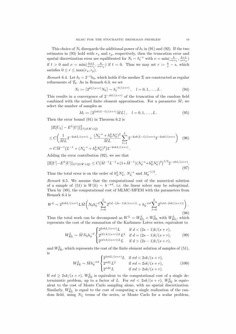
MLMC FOR THE STOCHASTIC BRINKMAN PROBLEM 19
This choice of Nl disregards the additional power of hl in (91) and (92). If the twoestimates in (93) hold with ru and rp, respectively, then the truncation error andspatial discretization error are equilibrated for Nl 0 h&(
l with / = min( ks+ru
, k+1s+rp
)if t > 0 and / = min( k+1
s+ru, k
s+rp) if t = 0. Thus we may set r := k
( ( s, whichsatisfies 0 # r # max(ru, rp).
Remark 6.4. Let hl = 2&lh0, which holds if the meshes Tl are constructed as regularrefinements of T0. As in Remark 6.3, we set
Nl := 12kl/(s+r)N02 0 h&k/(s+r)l , l = 0, 1, . . . , L . (94)
This results in a convergence of 2&skl/(s+r) of the truncation of the random fieldcombined with the mixed finite element approximation. For a parameter M , weselect the number of samples as
Ml := 122sk(L&l)/(s+r)ML2 , l = 0, 1, . . . , L . (95)
Then the error bound (91) in Theorem 6.2 is
*E[UL]( EL[U ]*2L2(";V %Q)
# C
51
ML2&2skL/(s+r) +
(N&s0 + hk
0Nr0 )2
ML
L+l=1
2&2sk(L&l)/(s+r)2&2skl/(s+r)
6= CM&1
&L&1 + (N&s
0 + hk0Nr
0 )2'2&2skL/(s+r) .
(96)
Adding the error contribution (92), we see that
*E[U ](EL[U ]*L2(";V %Q) # C&M&1L&1+(1+M&1)(N&s
0 +hk0Nr
0 )2'1/22&skL/(s+r).
(97)Thus the total error is on the order of hk
LNrL, N&s
L and M&1/20 .
Remark 6.5. We assume that the computational cost of the numerical solutionof a sample of (51) is W (h) 0 h&'d, i.e. the linear solver may be suboptimal.Then by (89), the computational cost of MLMC-MFEM with the parameters fromRemark 6.4 is
WL 0 22skL/(s+r)LM
5N0h
&d0
L+l=0
2l(d&(2s&1)k/(s+r)) + h&'d0
L+l=0
2l('d&2sk/(s+r))
6.
(98)Thus the total work can be decomposed as WL = WL
KL + WLFE with WL
KL, whichrepresents the cost of the summation of the Karhunen–Loeve series, equivalent to
WLKL 0 MN0h
&d0
@ABAC22skL/(s+r)L if d < (2s( 1)k/(s + r),2(d+k/(s+r))LL2 if d = (2s( 1)k/(s + r),2(d+k/(s+r))LL if d > (2s( 1)k/(s + r),
(99)
and WLFE, which represents the cost of the finite element solution of samples of (51),
is
WLFE 0 Mh&'d
0
@ABAC22skL/(s+r)L if -d < 2sk/(s + r),2'dLL2 if -d = 2sk/(s + r),2'dLL if -d > 2sk/(s + r).
(100)
If -d ' 2sk/(s + r), WLFE is equivalent to the computational cost of a single de-
terministic problem, up to a factor of L. For -d < 2sk/(s + r), WLFE is equiv-
alent to the cost of Monte Carlo sampling alone, with no spatial discretization.Similarly, WL
KL is equal to the cost of computing a single realization of the ran-dom field, using NL terms of the series, or Monte Carlo for a scalar problem,
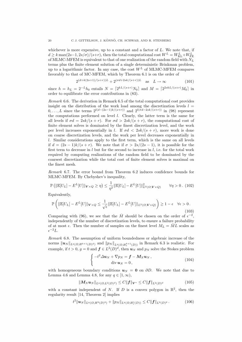
20 C. J. GITTELSON, J. KONNO, CH. SCHWAB, AND R. STENBERG
whichever is more expensive, up to a constant and a factor of L. We note that, ifd ' k max(2s(1, 2s/-)/(s+r), then the total computational cost WL = WL
KL+WLFE
of MLMC-MFEM is equivalent to that of one realization of the random field with NL
terms plus the finite element solution of a single deterministic Brinkman problem,up to a logarithmic factor. In any case, the cost WL of MLMC-MFEM comparesfavorably to that of MC-MFEM, which by Theorem 6.1 is on the order of
2(d+k(2s+1)/(s+r))L + 2('d+2sk/(s+r))L as L !$ (101)
since h = hL = 2&Lh0 entails N = 12kL/(s+r)N02 and M = 122skL/(s+r)M02 inorder to equilibrate the error contributions in (83).
Remark 6.6. The derivation in Remark 6.5 of the total computational cost providesinsight on the distribution of the work load among the discretization levels l =0, . . . , L since the terms 2l(d&(2s&1)k/(s+r)) and 2l('d&2sk/(s+r)) in (98) representthe computations performed on level l. Clearly, the latter term is the same forall levels if -d = 2sk/(s + r). For -d > 2sk/(s + r), the computational cost offinite element solves is dominated by the finest discretization level, and the workper level increases exponentially in l. If -d < 2sk/(s + r), more work is doneon coarse discretization levels, and the work per level decreases exponentially inl. Similar considerations apply to the first term, which is the same on all levelsif d = (2s ( 1)k/(s + r). We note that if - > 2s/(2s ( 1), it is possible for thefirst term to decrease in l but for the second to increase in l, i.e. for the total workrequired by computing realizations of the random field to be dominated by thecoarsest discretization while the total cost of finite element solves is maximal onthe finest mesh.
Remark 6.7. The error bound from Theorem 6.2 induces confidence bounds forMLMC-MFEM. By Chebyshev’s inequality,
P&*E[UL]( EL[U ]*V %Q ' 0
' # 102*E[UL](EL[U ]*2L2(";V %Q) -0 > 0 . (102)
Equivalently,
P5*E[UL]( EL[U ]*V %Q # 1/
6*E[UL]( EL[U ]*L2(";V %Q)
6' 1( 6 -6 > 0 .
(103)Comparing with (96), we see that the M should be chosen on the order of 6&2,independently of the number of discretization levels, to ensure a failure probabilityof at most 6. Then the number of samples on the finest level ML = ML scales as6&2L.
Remark 6.8. The assumption of uniform boundedness or algebraic increase of thenorms *uN*Lq(";Hk+1(D)d) and *pN*Lq(";Hk+1
! (D)) in Remark 6.3 is realistic. Forexample, if t > 0, g = 0 and f & L2(D)d, then uN and pN solve the Stokes problem!
(t27uN +)pN = f (MNuN ,
div uN = 0 ,(104)
with homogeneous boundary conditions uN = 0 on #D. We note that due toLemma 4.6 and Lemma 4.8, for any q & [1,$),
*MNuN*Lq(";L2(D)d) # C*f*V ! # C*f*L2(D)d (105)
with a constant independent of N . If D is a convex polygon in R2, then theregularity result [14, Theorem 2] implies
t2*uN*Lq(";H2(D)2) + *pN*Lq(";H1!(D)) # C*f*L2(D)2 . (106)

MLMC FOR THE STOCHASTIC BRINKMAN PROBLEM 21
Thus ru = 0 for k = 1 in Remark 6.3, and we may set r = 0 provided that rp # s,making use of the additional factor of hl in (91) and (92). Similar regularity resultsfor polyhedral domains in three dimensions are given in [8].
Remark 6.9. For the case t = 0, it is also realistic to expect algebraic growthin (93). For example, for f = 0, uN = (M&1
N )pN , and therefore pN is thesolution of ( div(M&1
N )pN ) = g on D and (M&1N )pN ) ·n = 0 on #D. We assume
for simplicity that each #n is a scalar function multiplied by the identity matrix.Then we have
(7pN = MNg + MN)M&1N ·)pN . (107)
By similar arguments as in the proof of Theorem 4.4, it can be shown that?????N+
n=1
Yn)#n
?????Lq(";L"(D)d)
# C
5 N+n=1
|#n|2(1&&)W 1,"(D)*#n*2&
W 2,"(D)
61/2
(108)
for any q & [1,$) and , & (0, 1). If D is a convex domain, using (22) andLemma 4.8, it follows that
*pN*Lq(";H2!(D)) # C
(1 +5 N+
n=1
|#n|2(1&&)W 1,"(D)*#n*2&
W 2,"(D)
61/2**g*L2(D) . (109)
In many examples, such as the model problem from Section 7 below, the right handside of (109) is either uniformly bounded in N or grows algebraically in N .
7. Numerical computations
In the following we verify the performance of the MLMC-MFEM method withnumerical examples in R2. The physical domain D is chosen as D = [(1, 1]%[(1, 1].We load the problem with boundary conditions only, thus g = 0 and f = 0. Bychoosing Dirichlet boundary data
uD = )(r) sin(18)) (110)
in polar coordinates (r, 8), we have uD & [H)(D)]d and for the boundary traceit holds uD|+D & [H)&1/2(#D)]d. The boundary conditions are enforced usingNitsche’s method, cf. [13]. Thus the norm for the velocity becomes
*v*2t,h := *v*2t + t2+
E$+Eh
1hE*[[v]]*20,E , (111)
in which #Eh denotes the collection of edges residing on the boundary #D. In allof the numerical examples we choose 1 = 3.1 to ensure su!cient regularity of theboundary data.
In the following we assume for simplicity the stochastic permeability matrix Mto be isotropic, lognormal, i.e.
M(x, 3) = exp(m(x, 3))I, (112)
in which m is an R-valued Gaussian field on D and m(x, 3) & L!(D, R). Forpractical applications, such as oil reservoir simulation, the permeability is usuallyof this diagonal form, and thus the test case is also of practical importance.
7.1. Karhunen–Loeve eigenpairs. To compute the eigenpairs of the truncatedKarhunen–Loeve expansion (29) numerically, one could employ e.g. finite elementmethods [18]. For simplicity, we only consider analytically known eigenexpansionsfor the Karhunen–Loeve series. We use the following result in one space dimensionas a basis.
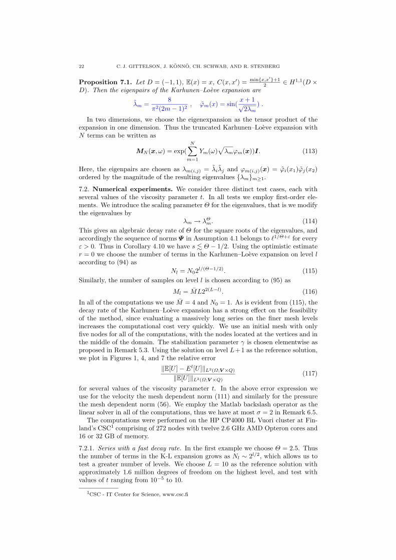
22 C. J. GITTELSON, J. KONNO, CH. SCHWAB, AND R. STENBERG
Proposition 7.1. Let D = ((1, 1), E(x) = x, C(x, x') = minx,x&+12 & H1,1(D %
D). Then the eigenpairs of the Karhunen–Loeve expansion are
&m =8
.2(2m( 1)2, 8m(x) = sin(
x + 1/2&m
) .
In two dimensions, we choose the eigenexpansion as the tensor product of theexpansion in one dimension. Thus the truncated Karhunen–Loeve expansion withN terms can be written as
MN (x, 3) = exp(N+
m=1
Ym(3),
&m8m(x))I. (113)
Here, the eigenpairs are chosen as &m(i,j) = &i&j and 8m(i,j)(x) = 8i(x1)8j(x2)ordered by the magnitude of the resulting eigenvalues &mm(1.
7.2. Numerical experiments. We consider three distinct test cases, each withseveral values of the viscosity parameter t. In all tests we employ first-order ele-ments. We introduce the scaling parameter 5 for the eigenvalues, that is we modifythe eigenvalues by
&m ! &,m. (114)
This gives an algebraic decay rate of 5 for the square roots of the eigenvalues, andaccordingly the sequence of norms # in Assumption 4.1 belongs to )1/,+- for every! > 0. Thus in Corollary 4.10 we have s " 5 ( 1/2. Using the optimistic estimater = 0 we choose the number of terms in the Karhunen–Loeve expansion on level laccording to (94) as
Nl = N02l/(,&1/2). (115)Similarly, the number of samples on level l is chosen according to (95) as
Ml = ML22(L&l). (116)
In all of the computations we use M = 4 and N0 = 1. As is evident from (115), thedecay rate of the Karhunen–Loeve expansion has a strong e"ect on the feasibilityof the method, since evaluating a massively long series on the finer mesh levelsincreases the computational cost very quickly. We use an initial mesh with onlyfive nodes for all of the computations, with the nodes located at the vertices and inthe middle of the domain. The stabilization parameter 2 is chosen elementwise asproposed in Remark 5.3. Using the solution on level L+1 as the reference solution,we plot in Figures 1, 4, and 7 the relative error
*E[U ]( El[U ]*L2(";V %Q)
*E[U ]*L2(";V %Q)(117)
for several values of the viscosity parameter t. In the above error expression weuse for the velocity the mesh dependent norm (111) and similarly for the pressurethe mesh dependent norm (56). We employ the Matlab backslash operator as thelinear solver in all of the computations, thus we have at most - = 2 in Remark 6.5.
The computations were performed on the HP CP4000 BL Vuori cluster at Fin-land’s CSC1 comprising of 272 nodes with twelve 2.6 GHz AMD Opteron cores and16 or 32 GB of memory.
7.2.1. Series with a fast decay rate. In the first example we choose 5 = 2.5. Thusthe number of terms in the K-L expansion grows as Nl 0 2l/2, which allows us totest a greater number of levels. We choose L = 10 as the reference solution withapproximately 1.6 million degrees of freedom on the highest level, and test withvalues of t ranging from 10&5 to 10.
1CSC - IT Center for Science, www.csc.fi
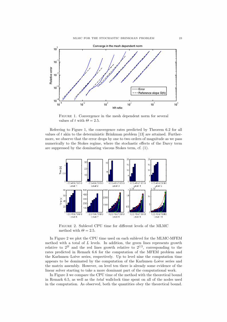
MLMC FOR THE STOCHASTIC BRINKMAN PROBLEM 23
Figure 1. Convergence in the mesh dependent norm for severalvalues of t with 5 = 2.5.
Referring to Figure 1, the convergence rates predicted by Theorem 6.2 for allvalues of t akin to the deterministic Brinkman problem [13] are attained. Further-more, we observe that the error drops by one to two orders of magnitude as we passnumerically to the Stokes regime, where the stochastic e"ects of the Darcy termare suppressed by the dominating viscous Stokes term, cf. (1).
Figure 2. Sublevel CPU time for di"erent levels of the MLMCmethod with 5 = 2.5.
In Figure 2 we plot the CPU time used on each sublevel for the MLMC-MFEMmethod with a total of L levels. In addition, the green lines represents growthrelative to 22l and the red lines growth relative to 2l/2, corresponding to therates predicted in Remark 6.6 for the computation of the MFEM problem andthe Karhunen–Loeve series, respectively. Up to level nine the computation timeappears to be dominated by the computation of the Karhunen–Loeve series andthe matrix assembly. However, on level ten there is already some evidence of thelinear solver starting to take a more dominant part of the computational work.
In Figure 3 we compare the CPU time of the method with the theoretical boundin Remark 6.5, as well as the total wallclock time spent on all of the nodes usedin the computation. As observed, both the quantities obey the theoretical bound.
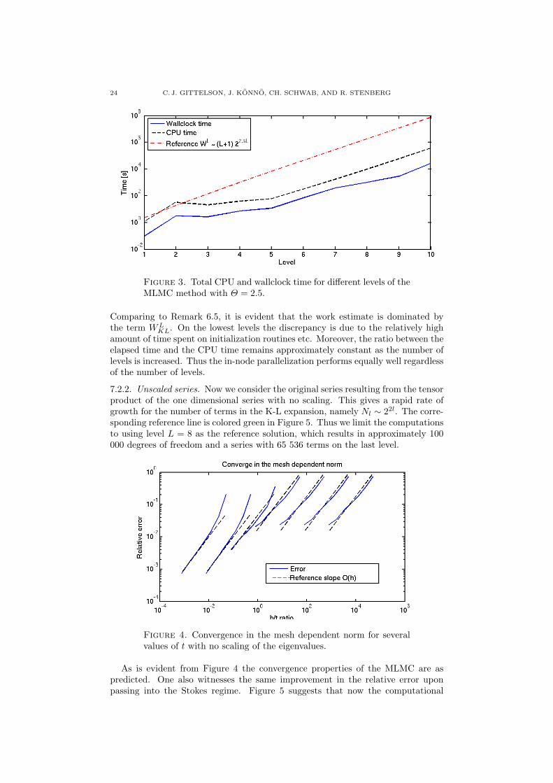
24 C. J. GITTELSON, J. KONNO, CH. SCHWAB, AND R. STENBERG
Figure 3. Total CPU and wallclock time for di"erent levels of theMLMC method with 5 = 2.5.
Comparing to Remark 6.5, it is evident that the work estimate is dominated bythe term WL
KL. On the lowest levels the discrepancy is due to the relatively highamount of time spent on initialization routines etc. Moreover, the ratio between theelapsed time and the CPU time remains approximately constant as the number oflevels is increased. Thus the in-node parallelization performs equally well regardlessof the number of levels.
7.2.2. Unscaled series. Now we consider the original series resulting from the tensorproduct of the one dimensional series with no scaling. This gives a rapid rate ofgrowth for the number of terms in the K-L expansion, namely Nl 0 22l. The corre-sponding reference line is colored green in Figure 5. Thus we limit the computationsto using level L = 8 as the reference solution, which results in approximately 100000 degrees of freedom and a series with 65 536 terms on the last level.
Figure 4. Convergence in the mesh dependent norm for severalvalues of t with no scaling of the eigenvalues.
As is evident from Figure 4 the convergence properties of the MLMC are aspredicted. One also witnesses the same improvement in the relative error uponpassing into the Stokes regime. Figure 5 suggests that now the computational
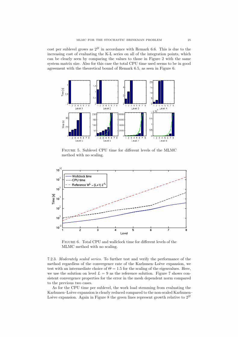
MLMC FOR THE STOCHASTIC BRINKMAN PROBLEM 25
cost per sublevel grows as 22l in accordance with Remark 6.6. This is due to theincreasing cost of evaluating the K-L series on all of the integration points, whichcan be clearly seen by comparing the values to those in Figure 2 with the samesystem matrix size. Also for this case the total CPU time used seems to be in goodagreement with the theoretical bound of Remark 6.5, as seen in Figure 6.
Figure 5. Sublevel CPU time for di"erent levels of the MLMCmethod with no scaling.
Figure 6. Total CPU and wallclock time for di"erent levels of theMLMC method with no scaling.
7.2.3. Moderately scaled series. To further test and verify the performance of themethod regardless of the convergence rate of the Karhunen–Loeve expansion, wetest with an intermediate choice of 5 = 1.5 for the scaling of the eigenvalues. Here,we use the solution on level L = 9 as the reference solution. Figure 7 shows con-sistent convergence properties for the error in the mesh dependent norm comparedto the previous two cases.
As for the CPU time per sublevel, the work load stemming from evaluating theKarhunen–Loeve expansion is clearly reduced compared to the non-scaled Karhunen–Loeve expansion. Again in Figure 8 the green lines represent growth relative to 22l
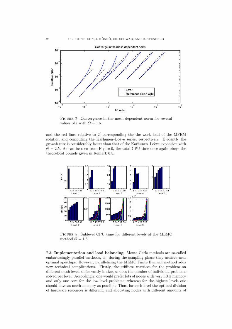
26 C. J. GITTELSON, J. KONNO, CH. SCHWAB, AND R. STENBERG
Figure 7. Convergence in the mesh dependent norm for severalvalues of t with 5 = 1.5.
and the red lines relative to 2l corresponding the the work load of the MFEMsolution and computing the Karhunen–Loeve series, respectively. Evidently thegrowth rate is considerably faster than that of the Karhunen–Loeve expansion with5 = 2.5. As can be seen from Figure 9, the total CPU time once again obeys thetheoretical bounds given in Remark 6.5.
Figure 8. Sublevel CPU time for di"erent levels of the MLMCmethod 5 = 1.5.
7.3. Implementation and load balancing. Monte Carlo methods are so-calledembarassingly parallel methods, ie. during the sampling phase they achieve nearoptimal speedups. However, parallelizing the MLMC Finite Element method addsnew technical complications. Firstly, the sti"ness matrices for the problem ondi"erent mesh levels di"er vastly in size, as does the number of individual problemssolved per level. Accordingly, one would prefer lots of nodes with very little memoryand only one core for the low-level problems, whereas for the highest levels oneshould have as much memory as possible. Thus, for each level the optimal divisionof hardware resources is di"erent, and allocating nodes with di"erent amounts of
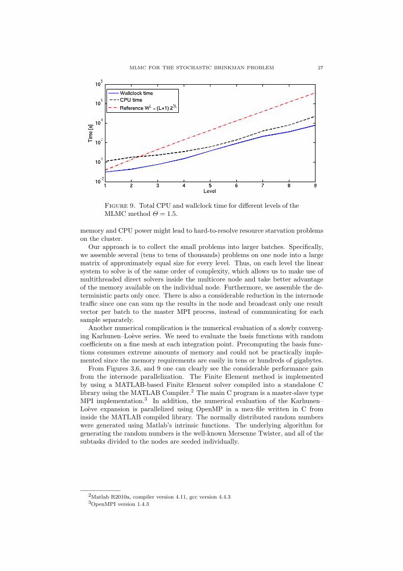
MLMC FOR THE STOCHASTIC BRINKMAN PROBLEM 27
Figure 9. Total CPU and wallclock time for di"erent levels of theMLMC method 5 = 1.5.
memory and CPU power might lead to hard-to-resolve resource starvation problemson the cluster.
Our approach is to collect the small problems into larger batches. Specifically,we assemble several (tens to tens of thousands) problems on one node into a largematrix of approximately equal size for every level. Thus, on each level the linearsystem to solve is of the same order of complexity, which allows us to make use ofmultithreaded direct solvers inside the multicore node and take better advantageof the memory available on the individual node. Furthermore, we assemble the de-terministic parts only once. There is also a considerable reduction in the internodetra!c since one can sum up the results in the node and broadcast only one resultvector per batch to the master MPI process, instead of communicating for eachsample separately.
Another numerical complication is the numerical evaluation of a slowly converg-ing Karhunen–Loeve series. We need to evaluate the basis functions with randomcoe!cients on a fine mesh at each integration point. Precomputing the basis func-tions consumes extreme amounts of memory and could not be practically imple-mented since the memory requirements are easily in tens or hundreds of gigabytes.
From Figures 3,6, and 9 one can clearly see the considerable performance gainfrom the internode parallelization. The Finite Element method is implementedby using a MATLAB-based Finite Element solver compiled into a standalone Clibrary using the MATLAB Compiler.2 The main C program is a master-slave typeMPI implementation.3 In addition, the numerical evaluation of the Karhunen–Loeve expansion is parallelized using OpenMP in a mex-file written in C frominside the MATLAB compiled library. The normally distributed random numberswere generated using Matlab’s intrinsic functions. The underlying algorithm forgenerating the random numbers is the well-known Mersenne Twister, and all of thesubtasks divided to the nodes are seeded individually.
2Matlab R2010a, compiler version 4.11, gcc version 4.4.33OpenMPI version 1.4.3
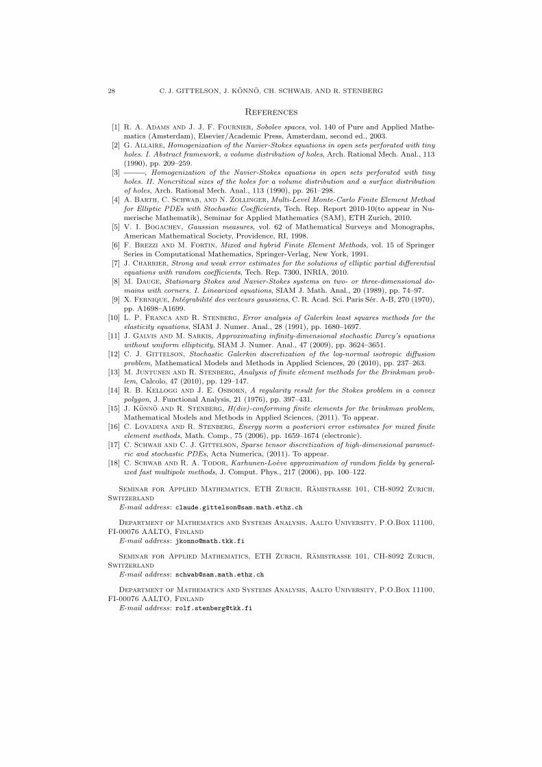
28 C. J. GITTELSON, J. KONNO, CH. SCHWAB, AND R. STENBERG
References
[1] R. A. Adams and J. J. F. Fournier, Sobolev spaces, vol. 140 of Pure and Applied Mathe-
matics (Amsterdam), Elsevier/Academic Press, Amsterdam, second ed., 2003.
[2] G. Allaire, Homogenization of the Navier-Stokes equations in open sets perforated with tinyholes. I. Abstract framework, a volume distribution of holes, Arch. Rational Mech. Anal., 113
(1990), pp. 209–259.
[3] , Homogenization of the Navier-Stokes equations in open sets perforated with tinyholes. II. Noncritical sizes of the holes for a volume distribution and a surface distribution
of holes, Arch. Rational Mech. Anal., 113 (1990), pp. 261–298.
[4] A. Barth, C. Schwab, and N. Zollinger, Multi-Level Monte-Carlo Finite Element Methodfor Elliptic PDEs with Stochastic Coe!cients, Tech. Rep. Report 2010-10(to appear in Nu-
merische Mathematik), Seminar for Applied Mathematics (SAM), ETH Zurich, 2010.
[5] V. I. Bogachev, Gaussian measures, vol. 62 of Mathematical Surveys and Monographs,American Mathematical Society, Providence, RI, 1998.
[6] F. Brezzi and M. Fortin, Mixed and hybrid Finite Element Methods, vol. 15 of SpringerSeries in Computational Mathematics, Springer-Verlag, New York, 1991.
[7] J. Charrier, Strong and weak error estimates for the solutions of elliptic partial di"erential
equations with random coe!cients, Tech. Rep. 7300, INRIA, 2010.[8] M. Dauge, Stationary Stokes and Navier-Stokes systems on two- or three-dimensional do-
mains with corners. I. Linearized equations, SIAM J. Math. Anal., 20 (1989), pp. 74–97.
[9] X. Fernique, Integrabilite des vecteurs gaussiens, C. R. Acad. Sci. Paris Ser. A-B, 270 (1970),pp. A1698–A1699.
[10] L. P. Franca and R. Stenberg, Error analysis of Galerkin least squares methods for the
elasticity equations, SIAM J. Numer. Anal., 28 (1991), pp. 1680–1697.[11] J. Galvis and M. Sarkis, Approximating infinity-dimensional stochastic Darcy’s equations
without uniform ellipticity, SIAM J. Numer. Anal., 47 (2009), pp. 3624–3651.
[12] C. J. Gittelson, Stochastic Galerkin discretization of the log-normal isotropic di"usionproblem, Mathematical Models and Methods in Applied Sciences, 20 (2010), pp. 237–263.
[13] M. Juntunen and R. Stenberg, Analysis of finite element methods for the Brinkman prob-lem, Calcolo, 47 (2010), pp. 129–147.
[14] R. B. Kellogg and J. E. Osborn, A regularity result for the Stokes problem in a convex
polygon, J. Functional Analysis, 21 (1976), pp. 397–431.[15] J. Konno and R. Stenberg, H(div)-conforming finite elements for the brinkman problem,
Mathematical Models and Methods in Applied Sciences, (2011). To appear.
[16] C. Lovadina and R. Stenberg, Energy norm a posteriori error estimates for mixed finiteelement methods, Math. Comp., 75 (2006), pp. 1659–1674 (electronic).
[17] C. Schwab and C. J. Gittelson, Sparse tensor discretization of high-dimensional paramet-
ric and stochastic PDEs, Acta Numerica, (2011). To appear.[18] C. Schwab and R. A. Todor, Karhunen-Loeve approximation of random fields by general-
ized fast multipole methods, J. Comput. Phys., 217 (2006), pp. 100–122.
Seminar for Applied Mathematics, ETH Zurich, Ramistrasse 101, CH-8092 Zurich,Switzerland
E-mail address: [email protected]
Department of Mathematics and Systems Analysis, Aalto University, P.O.Box 11100,FI-00076 AALTO, Finland
E-mail address: [email protected]
Seminar for Applied Mathematics, ETH Zurich, Ramistrasse 101, CH-8092 Zurich,
Switzerland
E-mail address: [email protected]
Department of Mathematics and Systems Analysis, Aalto University, P.O.Box 11100,
FI-00076 AALTO, FinlandE-mail address: [email protected]
Research Reports
No. Authors/Title
11-31 C.J. Gittelson, J. Konno, Ch. Schwab and R. StenbergThe multi-level Monte Carlo Finite Element Method for a stochasticBrinkman problem
11-30 A. Barth, A. Lang and Ch. SchwabMulti-level Monte Carlo Finite Element method for parabolic stochasticpartial di!erential equations
11-29 M. Hansen and Ch. SchwabAnalytic regularity and nonlinear approximation of a class of parametricsemilinear elliptic PDEs
11-28 R. Hiptmair and S. MaoStable multilevel splittings of boundary edge element spaces
11-27 Ph. GrohsShearlets and microlocal analysis
11-26 H. KumarImplicit-explicit Runge-Kutta methods for the two-fluid MHD equations
11-25 H. Papasaika, E. Kokiopoulou, E. Baltsavias, K. Schindler andD. KressnerSparsity-seeking fusion of digital elevation models
11-24 H. Harbrecht and J. LiA fast deterministic method for stochastic elliptic interface problemsbased on low-rank approximation
11-23 P. Corti and S. MishraStable finite di!erence schemes for the magnetic induction equation withHall e!ect
11-22 H. Kumar and S. MishraEntropy stable numerical schemes for two-fluid MHD equations
11-21 H. Heumann, R. Hiptmair, K. Li and J. XuSemi-Lagrangian methods for advection of di!erential forms
11-20 A. MoiolaPlane wave approximation in linear elasticity
11-19 C.J. GittelsonUniformly convergent adaptive methods for parametric operatorequations
11-18 E. Kokiopoulou, D. Kressner, M. Zervos and N. ParagiosOptimal similarity registration of volumetric images