Finite Element Approximations of Burgers' Equation - Virginia Tech

FINITE ELEMENT APPROXIMATIONS OF

BURGERS’ EQUATION WITH ROBIN’S

BOUNDARY CONDITIONS

by

Lyle C. Smith III

Thesis submitted to the faculty of the

Virginia Polytechnic Institute and State University

in partial fulfillment of the requirements for the degree of

MASTER OF SCIENCE

in

Mathematics

APPROVED:

John A. Burns, Chairman

Terry L. Herdman Robert C. Rogers

July, 1997

Blacksburg, Virginia

FINITE ELEMENT APPROXIMATIONS OF BURGERS’

EQUATION WITH ROBIN’S BOUNDARY CONDITIONS

by

Lyle C. Smith III

Committee Chairman: John A. Burns

Mathematics

(ABSTRACT)

This work is a numerical study of Burgers’ equation with Robin’s boundary conditions.

The goal is to determine the behavior of the solutions in the limiting cases of Dirichlet and

Neumann boundary conditions. We develop and test two separate finite element and Galerkin

schemes. The Galerkin/Conservation method is shown to give better results and is then used to

compute the response as the Robin’s Boundary conditions approach both the Dirichlet and

Neumann boundary conditions. Burgers’ equation is treated as a perturbation of the linear heat

equation with the appropriate realistic constants.

The goal is to determine if the use of the Robin’s boundary conditions to approximate

Dirichlet and Neumann boundary conditions affords any advantage over schemes that employ only

“exact” Dirichlet or Neumann boundary conditions. Our finite element results indicate that

solutions using appropriate Robin’s boundary conditions approach the same solutions obtained by

“exact” Dirichlet or Neumann boundary conditions. This allows us to obtain realistic solutions in

some cases where the other schemes had previously failed.

iii

ACKNOWLEDGMENTS

I want to express my gratitude to my friend, advisor, and thesis committee chairman Dr.

John Burns. His encouragement, guidance, and insight have been invaluable both with this thesis

and also with my undergraduate and graduate studies. I would also like to thank Dr. Terry

Herdman and Dr. Robert Rogers for serving on my thesis committee and for their help throughout

my years at Virginia Tech. The enthusiasm and insight of these three men has made my pursuit of

mathematics both fun and rewarding.

I would like to acknowledge the financial support I received from the Air Force Office of

Scientific Research under Grant F49620-96-1-0329 and the Center for Transportation Research.

Many thanks also to my companions Tom Bail and Shana Olds. They have been an

encouragement for over five years as we have persevered together first through undergraduate

school and now finishing our Masters’ degrees. They have served as models of hard work and

dedication. Thanks to Ken Massa as well for his patience and determination as we finished our

theses together this summer.

Finally, I would like to express my deepest gratitude to Jesus Christ, my Creator,

Redeemer, and Friend. I am forever indebted to Him for revealing to me true spiritual wisdom

and mathematical insight. I look forward to spending eternity thanking Him face-to-face.

iv

TABLE OF CONTENTS

1 INTRODUCTION

1.1 Introduction . . . . . . . . . . . . . . . . . . . . . . . . . . . . . . . . . . . . . . . . . . . . . . . . . . . . . . 1

1.2 The Heat Equation . . . . . . . . . . . . . . . . . . . . . . . . . . . . . . . . . . . . . . . . . . . . . . . . . 2

1.3 Robin’s Boundary Conditions . . . . . . . . . . . . . . . . . . . . . . . . . . . . . . . . . . . . . . . . . 7

1.4 The Burgers’ Equation . . . . . . . . . . . . . . . . . . . . . . . . . . . . . . . . . . . . . . . . . . . . . . 9

1.5 Perspective . . . . . . . . . . . . . . . . . . . . . . . . . . . . . . . . . . . . . . . . . . . . . . . . . . . . . . 12

1.6 Goals . . . . . . . . . . . . . . . . . . . . . . . . . . . . . . . . . . . . . . . . . . . . . . . . . . . . . . . . . . 14

2 THE FINITE ELEMENT METHOD

2.1 A Review of the Equations . . . . . . . . . . . . . . . . . . . . . . . . . . . . . . . . . . . . . . . . . . 15

2.2 The Galerkin Method and the Weak Form . . . . . . . . . . . . . . . . . . . . . . . . . . . . . . . 16

2.3 The Finite Element Approximation . . . . . . . . . . . . . . . . . . . . . . . . . . . . . . . . . . . . 16

2.4 The Galerkin/Conservation Method . . . . . . . . . . . . . . . . . . . . . . . . . . . . . . . . . . . . 23

3 NUMERICAL RESULTS

3.1 Setting Up the Problem . . . . . . . . . . . . . . . . . . . . . . . . . . . . . . . . . . . . . . . . . . . . . 26

3.2 A Comparison to Known Solutions . . . . . . . . . . . . . . . . . . . . . . . . . . . . . . . . . . . . 28

3.3 A Comparison to Previous Work . . . . . . . . . . . . . . . . . . . . . . . . . . . . . . . . . . . . . . 53

3.4 Results Approaching Dirichlet Boundary Conditions . . . . . . . . . . . . . . . . . . . . . . . 61

3.5 Results Approaching Neumann Boundary Conditions . . . . . . . . . . . . . . . . . . . . . . 73

4 CONCLUSIONS

4.1 Overview of Results . . . . . . . . . . . . . . . . . . . . . . . . . . . . . . . . . . . . . . . . . . . . . . . .85

4.2 Conclusions . . . . . . . . . . . . . . . . . . . . . . . . . . . . . . . . . . . . . . . . . . . . . . . . . . . . . . 86

4.3 Open Problems . . . . . . . . . . . . . . . . . . . . . . . . . . . . . . . . . . . . . . . . . . . . . . . . . . . .87

A MATLAB CODE . . . . . . . . . . . . . . . . . . . . . . . . . . . . . . . . . . . . . . . . . . . . . . . . . . . . .88

v

LIST OF FIGURES

1.2.1 A heat conducting rod . . . . . . . . . . . . . . . . . . . . . . . . . . . . . . . . . . . . . . . . . . . . . . . . . . . 2

1.3.1 A uniform rod with films and heating elements . . . . . . . . . . . . . . . . . . . . . . . . . . . . . . . . . 7

1.4.1 A typical solution of w(t,x)w (t,x) = gw (t,x) . . . . . . . . . . . . . . . . . . . . . . . . . . . . . . . . 11x xx

3.2.1 Exact Solution for a 1m copper rod with 10cm aluminum films; . . . . . . . . . . . . . . . . . . . 35w(t,x) = e [Ax + Bx + C + sin (.01Bx)].-.3t 2 2

3.2.2 Galerkin method, N=4, 1m copper rod with 10cm aluminum films; . . . . . . . . . . . . . . . . . 36w(t,x) = e [Ax + Bx + C + sin (.01Bx)]; a) Numerical Solution b) Error.-.3t 2 2

3.2.3 Galerkin method, N=8, 1m copper rod with 10cm aluminum films; . . . . . . . . . . . . . . . . . 37w(t,x) = e [Ax + Bx + C + sin (.01Bx)]; a) Numerical Solution b) Error.-.3t 2 2

3.2.4 Galerkin method, N=16, 1m copper rod with 10cm aluminum films; . . . . . . . . . . . . . . . . 38w(t,x) = e [Ax + Bx + C + sin (.01Bx)]; a) Numerical Solution b) Error.-.3t 2 2

3.2.5 Galerkin method, N=32, 1m copper rod with 10cm aluminum films; . . . . . . . . . . . . . . . . 39w(t,x) = e [Ax + Bx + C + sin (.01Bx)]; a) Numerical Solution b) Error.-.3t 2 2

3.2.6 Galerkin/Conservation method, N=4, 1m copper rod with 10cm aluminum films; . . . . . . 40w(t,x) = e [Ax + Bx + C + sin (.01Bx)]; a) Numerical Solution b) Error.-.3t 2 2

3.2.7 Galerkin/Conservation method, N=8, 1m copper rod with 10cm aluminum films; . . . . . . 41w(t,x) = e [Ax + Bx + C + sin (.01Bx)]; a) Numerical Solution b) Error.-.3t 2 2

3.2.8 Galerkin/Conservation method, N=16 , 1m copper rod with 10cm aluminum films;. . . . . 42w(t,x) = e [Ax + Bx + C + sin (.01Bx)]; a) Numerical Solution b) Error.-.3t 2 2

3.2.9 Galerkin/Conservation method, N=32, 1m copper rod with 10cm aluminum films; . . . . . 43w(t,x) = e [Ax + Bx + C + sin (.01Bx)]; a) Numerical Solution b) Error.-.3t 2 2

3.2.10 Exact Solution for a 1m copper rod with 10cm aluminum films; . . . . . . . . . . . . . . . . . . 44w(t,x) = [(100-x)/100] sin(1.5Bt) + (x/100) cos(.5Bt).2 2

3.2.11 Galerkin method, N=4, 1m copper rod with 10cm aluminum films; . . . . . . . . . . . . . . . . 45w(t,x) = [(100-x)/100] sin(1.5Bt) + (x/100) cos(.5Bt); a) Numerical Solution b) Error.2 2

vi

3.2.12 Galerkin method, N=8, 1m copper rod with 10cm aluminum films; . . . . . . . . . . . . . . . . 46w(t,x) = [(100-x)/100] sin(1.5Bt) + (x/100) cos(.5Bt); a) Numerical Solution b) Error.2 2

3.2.13 Galerkin method, N=16, 1m copper rod with 10cm aluminum films; . . . . . . . . . . . . . . . 47w(t,x) = [(100-x)/100] sin(1.5Bt) + (x/100) cos(.5Bt); a) Numerical Solution b) Error.2 2

3.2.14 Galerkin method, N=32, 1m copper rod with 10cm aluminum films; . . . . . . . . . . . . . . . 48w(t,x) = [(100-x)/100] sin(1.5Bt) + (x/100) cos(.5Bt); a) Numerical Solution b) Error.2 2

3.2.15 Galerkin/Conservation method, N=4, 1m copper rod with 10cm aluminum films; . . . . . 49w(t,x) = [(100-x)/100] sin(1.5Bt) + (x/100) cos(.5Bt); a) Numerical Solution b) Error.2 2

3.2.16 Galerkin/Conservation method, N=8, 1m copper rod with 10cm aluminum films; . . . . . 50w(t,x) = [(100-x)/100] sin(1.5Bt) + (x/100) cos(.5Bt); a) Numerical Solution b) Error.2 2

3.2.17 Galerkin/Conservation method, N=16, 1m copper rod with 10cm aluminum films; . . . . 51w(t,x) = [(100-x)/100] sin(1.5Bt) + (x/100) cos(.5Bt); a) Numerical Solution b) Error.2 2

3.2.18 Galerkin/Conservation method, N=32, 1m copper rod with 10cm aluminum films; . . . . 52w(t,x) = [(100-x)/100] sin(1.5Bt) + (x/100) cos(.5Bt); a) Numerical Solution b) Error.2 2

3.3.1 w (x) = (1/16)cos(Bx) R =60: a) Galerkin method, b) Galerkin/Conservation method. . 550 E

3.3.2 w (x) = (1/16)cos(Bx) R =120: a) Galerkin method, b) Galerkin/Conservation method .560 E

3.3.3 w (x) = (1/16)cos(Bx) R =240: a) Galerkin method, b) Galerkin/Conservation method .570 E

3.3.4 w (x) = (½)cos(Bx) R =60: a) Galerkin method, b) Galerkin/Conservation method. . . 580 E

3.3.5 w (x) = (½)cos(Bx) R =120: a) Galerkin method, b) Galerkin/Conservation method. . 590 E

3.3.6 w (x) = (½)cos(Bx) R =240: a) Galerkin method, b) Galerkin/Conservation method. . 600 E

3.4.1 w (x) = (½)cos(.01Bx); 1m iron rod with 10cm copper films; Long term solution . . . . 640

3.4.2 w (x) = (½)cos(.01Bx); 1m iron rod with 10cm copper films. . . . . . . . . . . . . . . . . . . . .650

3.4.3 w (x) = (½)cos(.01Bx); 1m iron rod with 1cm copper films. . . . . . . . . . . . . . . . . . . . . .660

3.4.4 w (x) = (½)cos(.01Bx); 1m iron rod with 0.1cm copper films. . . . . . . . . . . . . . . . . . . . 670

3.4.5 w (x) = (½)cos(.01Bx); 1m iron rod with 0.01cm copper films. . . . . . . . . . . . . . . . . . . 680

vii

3.4.6 w (x) =.3sin(.01Bx); 1m aluminum rod with 10cm silver films; Long term solution . . . . 690

3.4.7 w (x) =.3sin(.01Bx); 1m aluminum rod with 10cm silver films. . . . . . . . . . . . . . . . . . . . .700

3.4.8 w (x) =.3sin(.01Bx); 1m aluminum rod with 1cm silver films. . . . . . . . . . . . . . . . . . . . . .710

3.4.9 w (x) =.3sin(.01Bx); 1m aluminum rod with 0.1cm silver films. . . . . . . . . . . . . . . . . . . . 720

3.5.1 w (x) =.4cos(.01Bx); 1m aluminum rod with Neumann boundaries. . . . . . . . . . . . . . . . . 750

3.5.2 w (x) =.4cos(.01Bx); 1m aluminum rod with 1m iron films. . . . . . . . . . . . . . . . . . . . . . . 760

3.5.3 w (x) =.4cos(.01Bx); 1m aluminum rod with 10m iron films. . . . . . . . . . . . . . . . . . . . . . 770

3.5.4 w (x) =.4cos(.01Bx); 1m aluminum rod with 100m iron films. . . . . . . . . . . . . . . . . . . . . 780

3.5.5 w (x) =.4cos(.01Bx); 1m aluminum rod with 100m iron films; Long term solution . . . . 790

3.5.6 w (x) =.4cos(.01Bx); 1m aluminum rod with 1000m iron films. . . . . . . . . . . . . . . . . . . . 800

3.5.7 w (x) =cos(.01Bx); 1m granite rod with Neumann boundaries. . . . . . . . . . . . . . . . . . . . .810

3.5.8 w (x) =cos(.01Bx); 1m granite rod with 10m iron films. . . . . . . . . . . . . . . . . . . . . . . . . .820

3.5.9 w (x) =cos(.01Bx); 1m granite rod with 100m iron films. . . . . . . . . . . . . . . . . . . . . . . . .830

3.5.10 w (x) =cos(.01Bx); 1m granite rod with 1000m iron films. . . . . . . . . . . . . . . . . . . . . . .840

viii

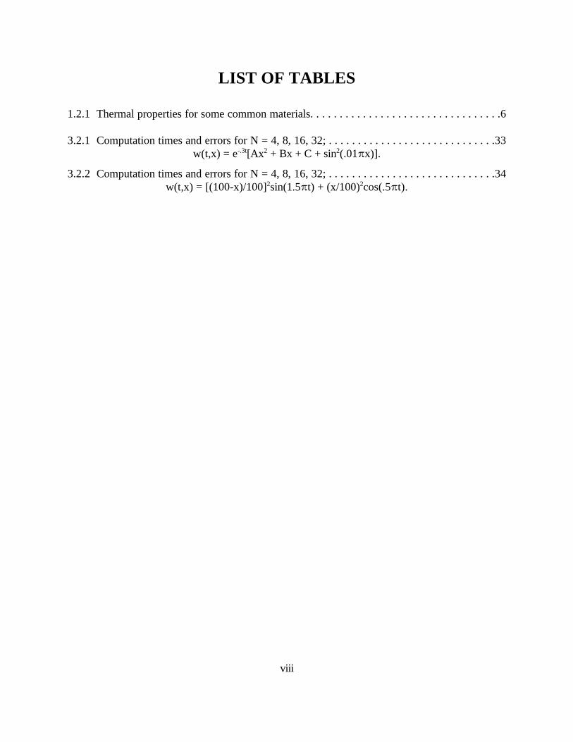
LIST OF TABLES

1.2.1 Thermal properties for some common materials. . . . . . . . . . . . . . . . . . . . . . . . . . . . . . . . .6

3.2.1 Computation times and errors for N = 4, 8, 16, 32; . . . . . . . . . . . . . . . . . . . . . . . . . . . . .33w(t,x) = e [Ax + Bx + C + sin (.01Bx)].-.3t 2 2

3.2.2 Computation times and errors for N = 4, 8, 16, 32; . . . . . . . . . . . . . . . . . . . . . . . . . . . . .34w(t,x) = [(100-x)/100] sin(1.5Bt) + (x/100) cos(.5Bt).2 2

1

Chapter One

INTRODUCTION

1.1 Introduction

In this thesis, we investigate the Burgers’ equation with Robin’s boundary conditions.

The Burgers’ equation is treated as a perturbation of the linear heat equation. We employ several

realistic boundary conditions. We develop two finite element schemes to solve this problem

numerically. Pugh [1] determined that the Galerkin/Conservation method was more accurate and

computed more quickly than the Galerkin method for the Burgers’ equation with Neumann

boundary conditions. We compare these two schemes for Robin’s boundary conditions. The

Galerkin/Conservation method is shown to be preferable and is therefore used to solve the

subsequent problems in this paper.

It is known that all steady state solutions of Burgers’ equation with homogeneous

Neumann boundary conditions are constant [2]. In this thesis, we study the behavior of the

Burgers’ equation with Robin’s boundary conditions. We let the Robin’s boundary conditions

approach homogeneous Neumann boundary conditions and compare the Neumann solution to the

asymptotic solution as Robin’s boundary conditions approach Neumann boundary conditions. We

also investigate asymptotic solutions as the Robin’s boundary conditions approach Dirichlet

boundary conditions.

F(t,x) ' &6 MwMx

(t,x)

2

1.2 The Heat Equation

Many engineering applications today rely on the dynamics of heat intensity and flow within

objects. From bridge I-beams to microprocessors, knowledge of the temperature and its transient

distribution is vital in design and implementation. Therefore we would like to be able to predict

the temperature of an object given a set of initial conditions and boundary conditions.

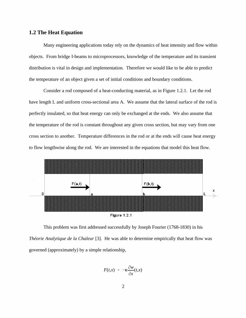
Consider a rod composed of a heat-conducting material, as in Figure 1.2.1. Let the rod

have length L and uniform cross-sectional area A. We assume that the lateral surface of the rod is

perfectly insulated, so that heat energy can only be exchanged at the ends. We also assume that

the temperature of the rod is constant throughout any given cross section, but may vary from one

cross section to another. Temperature differences in the rod or at the ends will cause heat energy

to flow lengthwise along the rod. We are interested in the equations that model this heat flow.

This problem was first addressed successfully by Joseph Fourier (1768-1830) in his

Théorie Analytique de la Chaleur [3]. He was able to determine empirically that heat flow was

governed (approximately) by a simple relationship,

Q(t) ' mb

a

w(t,x)D(x)c(x)Adx.

3

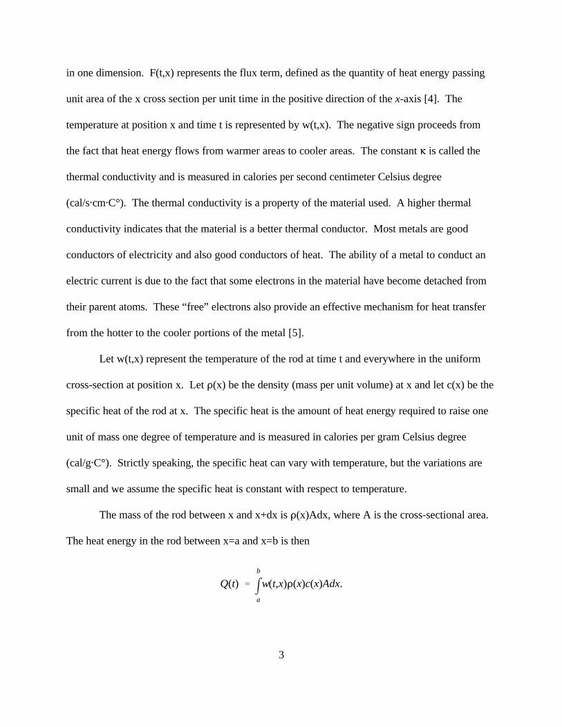
in one dimension. F(t,x) represents the flux term, defined as the quantity of heat energy passing

unit area of the x cross section per unit time in the positive direction of the x-axis [4]. The

temperature at position x and time t is represented by w(t,x). The negative sign proceeds from

the fact that heat energy flows from warmer areas to cooler areas. The constant 6 is called the

thermal conductivity and is measured in calories per second centimeter Celsius degree

(cal/s"cm"C°). The thermal conductivity is a property of the material used. A higher thermal

conductivity indicates that the material is a better thermal conductor. Most metals are good

conductors of electricity and also good conductors of heat. The ability of a metal to conduct an

electric current is due to the fact that some electrons in the material have become detached from

their parent atoms. These “free” electrons also provide an effective mechanism for heat transfer

from the hotter to the cooler portions of the metal [5].

Let w(t,x) represent the temperature of the rod at time t and everywhere in the uniform

cross-section at position x. Let D(x) be the density (mass per unit volume) at x and let c(x) be the

specific heat of the rod at x. The specific heat is the amount of heat energy required to raise one

unit of mass one degree of temperature and is measured in calories per gram Celsius degree

(cal/g"C°). Strictly speaking, the specific heat can vary with temperature, but the variations are

small and we assume the specific heat is constant with respect to temperature.

The mass of the rod between x and x+dx is D(x)Adx, where A is the cross-sectional area.

The heat energy in the rod between x=a and x=b is then

mb

a

f1(t,x) Adx.

flux term ' &A[F(t,b) & F(t,a)] ' A[6(b)MwMx

(t,b) & 6(a)MwMx

(t,a)]

' mb

a

A MMx

(6(x) MwMx

(t,x)) dx.

dQdt

' flux term % source term, or

mb

a

wt(t,x) D(x)c(x) Adx ' mb

a

MMx

(6(x)wx(t,x)) Adx % mb

a

f1(t,x) Adx,

Amb

a

[D(x)c(x)wt(t,x) &MMx

(6(x)wx(t,x)) & f(t,x)] dx ' 0.

4

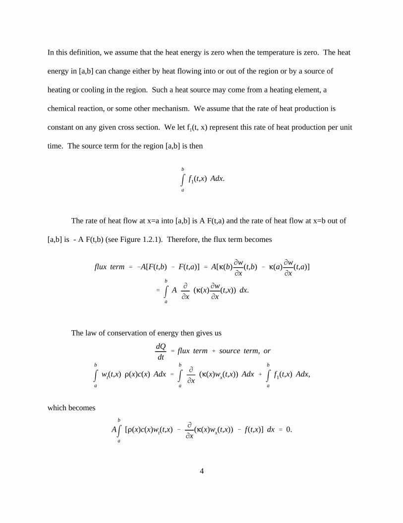
In this definition, we assume that the heat energy is zero when the temperature is zero. The heat

energy in [a,b] can change either by heat flowing into or out of the region or by a source of

heating or cooling in the region. Such a heat source may come from a heating element, a

chemical reaction, or some other mechanism. We assume that the rate of heat production is

constant on any given cross section. We let f (t, x) represent this rate of heat production per unit1

time. The source term for the region [a,b] is then

The rate of heat flow at x=a into [a,b] is A F(t,a) and the rate of heat flow at x=b out of

[a,b] is - A F(t,b) (see Figure 1.2.1). Therefore, the flux term becomes

The law of conservation of energy then gives us

which becomes

D(x)c(x) wt(t,x) 'MMx

(6(x) wx(t,x)) % f1(t,x).

MwMt

(t,x) ' g M2w

Mx 2(t,x) % f(t,x).

w(0,x) ' w0(x)

w(t,0)'u1(t) w(t,L)'u2(t) 0#x#L

5

(1.1.1)

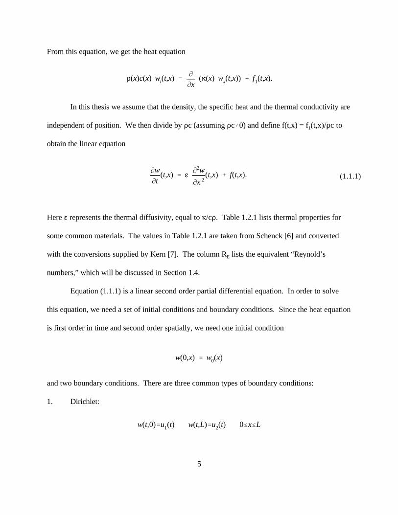
From this equation, we get the heat equation

In this thesis we assume that the density, the specific heat and the thermal conductivity are

independent of position. We then divide by Dc (assuming Dc…0) and define f(t,x) = f (t,x)/Dc to1

obtain the linear equation

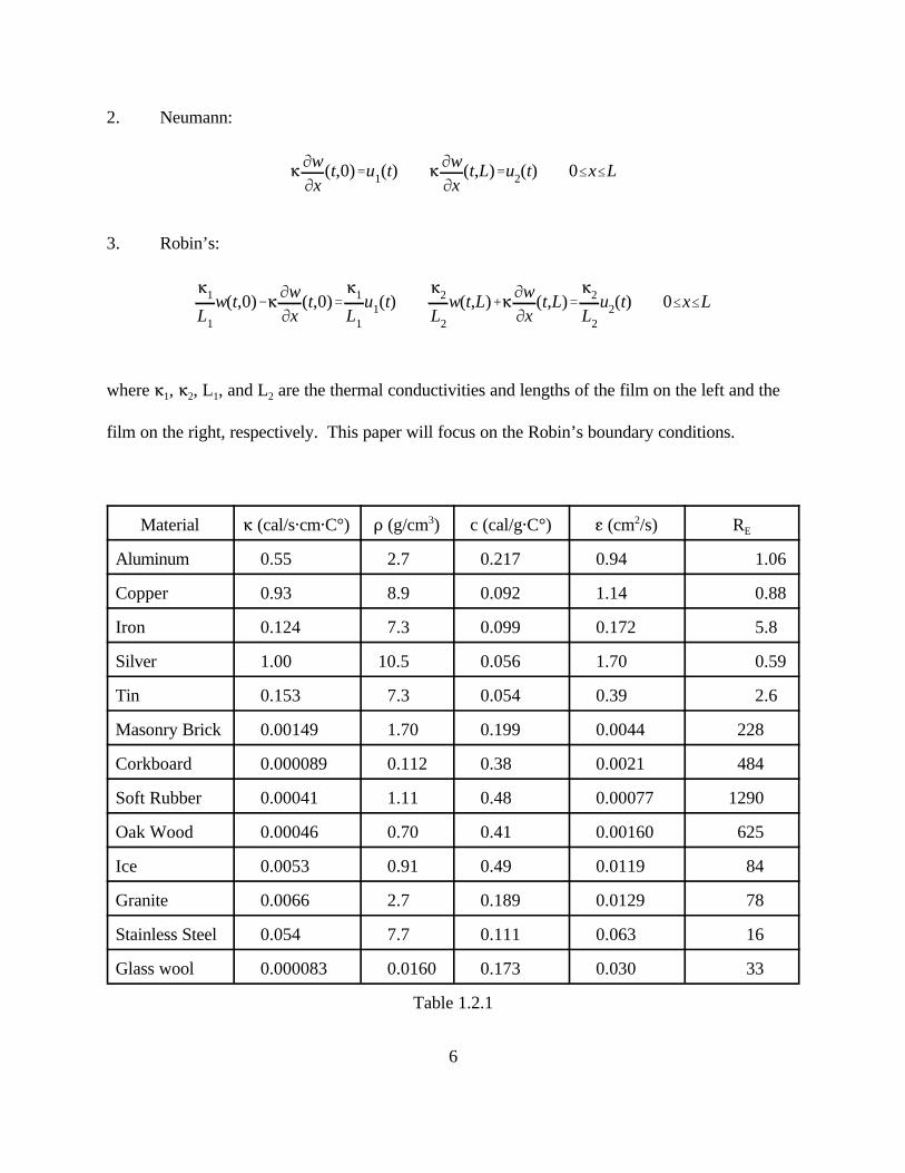
Here g represents the thermal diffusivity, equal to 6/cD. Table 1.2.1 lists thermal properties for

some common materials. The values in Table 1.2.1 are taken from Schenck [6] and converted

with the conversions supplied by Kern [7]. The column R lists the equivalent “Reynold’sE

numbers,” which will be discussed in Section 1.4.

Equation (1.1.1) is a linear second order partial differential equation. In order to solve

this equation, we need a set of initial conditions and boundary conditions. Since the heat equation

is first order in time and second order spatially, we need one initial condition

and two boundary conditions. There are three common types of boundary conditions:

1. Dirichlet:

6 MwMx

(t,0)'u1(t) 6 MwMx

(t,L)'u2(t) 0#x#L

61

L1

w(t,0)&6 MwMx

(t,0)'61

L1

u1(t)62

L2

w(t,L)%6 MwMx

(t,L)'62

L2

u2(t) 0#x#L

6

2. Neumann:

3. Robin’s:

where 6 , 6 , L , and L are the thermal conductivities and lengths of the film on the left and the1 2 1 2

film on the right, respectively. This paper will focus on the Robin’s boundary conditions.

Material 6 (cal/s"cm"C°) D (g/cm ) c (cal/g"C°) g (cm /s) R3 2E

Aluminum 0.55 2.7 0.217 0.94 1.06

Copper 0.93 8.9 0.092 1.14 0.88

Iron 0.124 7.3 0.099 0.172 5.8

Silver 1.00 10.5 0.056 1.70 0.59

Tin 0.153 7.3 0.054 0.39 2.6

Masonry Brick 0.00149 1.70 0.199 0.0044 228

Corkboard 0.000089 0.112 0.38 0.0021 484

Soft Rubber 0.00041 1.11 0.48 0.00077 1290

Oak Wood 0.00046 0.70 0.41 0.00160 625

Ice 0.0053 0.91 0.49 0.0119 84

Granite 0.0066 2.7 0.189 0.0129 78

Stainless Steel 0.054 7.7 0.111 0.063 16

Glass wool 0.000083 0.0160 0.173 0.030 33

Table 1.2.1

w(t,0) ' w1(t,0) 6 MwMx

(t,0) ' 61

Mw1

Mx(t,0).

film 2uniform rodfilm 1

0 L L+L2Figure 1.3.1

7

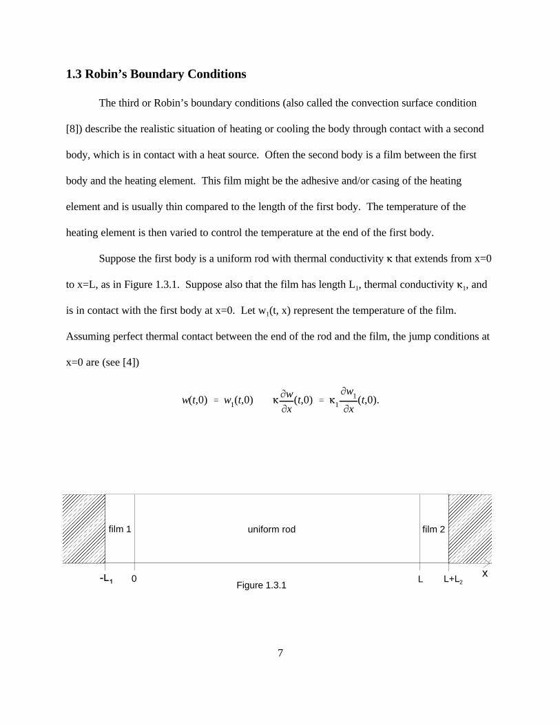
1.3 Robin’s Boundary Conditions

The third or Robin’s boundary conditions (also called the convection surface condition

[8]) describe the realistic situation of heating or cooling the body through contact with a second

body, which is in contact with a heat source. Often the second body is a film between the first

body and the heating element. This film might be the adhesive and/or casing of the heating

element and is usually thin compared to the length of the first body. The temperature of the

heating element is then varied to control the temperature at the end of the first body.

Suppose the first body is a uniform rod with thermal conductivity 6 that extends from x=0

to x=L, as in Figure 1.3.1. Suppose also that the film has length L , thermal conductivity 6 , and1 1

is in contact with the first body at x=0. Let w (t, x) represent the temperature of the film. 1

Assuming perfect thermal contact between the end of the rod and the film, the jump conditions at

x=0 are (see [4])

61

Mw1

Mx(t,0) ' 61

w1(t,&L1)&w1(t,0)

&L1

'61

&L1

(u1(t)&w(t,0)).

6 MwMx

(t,0) '61

&L1

(u1(t)&w(t,0))

61

L1

w(t,0) & 6 MwMx

(t,0) '61

L1

u1(t).

62

L2

w(t,L) % 6 MwMx

(t,L) '62

L2

u2(t).

8

At the other end of the film, the temperature of the film is equal to the temperature of the heat

source, w (t, -L ) = u (t).1 1 1

Newton’s law of “radiation” states that the heat flux is proportional to the temperature

difference between the two bodies [9]. Equivalently, we approximate the derivative Mw /Mx by the1

difference quotient,

The boundary condition at x=0 becomes

or equivalently,

Similarly, the boundary condition at x=L becomes

Again, 6 refers to the thermal conductivity of the rod and 6 and 6 refer to the thermal1 2

conductivities of films one and two respectively. The constants L and L are the thicknesses of1 2

films one and two respectively. A list of thermal conductivities and other thermal properties for

some common materials are given in Table 1.2.1.

MwMt

(t,x) % w(t,x)MwMx

(t,x) ' g M2w

Mx 2(t,x) % f(t,x),

9

(1.4.1)

1.4 The Burger’s Equation

The Burgers’ equation serves as a useful model for many interesting problems in applied

mathematics. It models effectively certain problems of a fluid flow nature, in which either shocks

or viscous dissipation is a significant factor.

The first steady-state solutions of Burgers’ equation were given by Bateman [10] in 1915.

However, the equation gets its name from the extensive research of Burgers [11] beginning in

1939. Burgers focussed on modeling turbulence, but the equation is useful for modeling such

diverse physical phenomena as shock flows, traffic flow, acoustic transmission in fog, etc. In

fact, it can be used as a model for any nonlinear wave propagation problem subject to dissipation

[12]. Depending on the problem being modeled, this dissipation may result from viscosity, heat

conduction, mass diffusion, thermal radiation, chemical reaction, or other source. We shall take

the point of view that Burgers’ equation is a perturbation of the linear heat equation. In

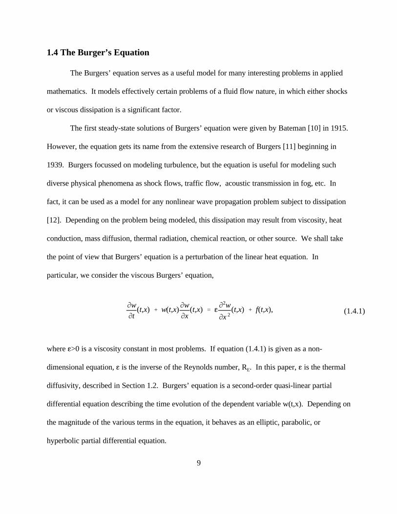
particular, we consider the viscous Burgers’ equation,

where g>0 is a viscosity constant in most problems. If equation (1.4.1) is given as a non-

dimensional equation, g is the inverse of the Reynolds number, R . In this paper, g is the thermalE

diffusivity, described in Section 1.2. Burgers’ equation is a second-order quasi-linear partial

differential equation describing the time evolution of the dependent variable w(t,x). Depending on

the magnitude of the various terms in the equation, it behaves as an elliptic, parabolic, or

hyperbolic partial differential equation.

wt(t,x) % w(t,x)wx(t,x) ' 0,

10

Burgers’ equation has not been solved in closed form, but for many combinations of initial

and boundary conditions, an exact solution can easily be found. Hopf [13] and Cole [14]

discovered a transformation that reduces the Burgers’ equation to the linear heat equation.

However, these solution are restricted, in most cases, to the infinite interval -4<x<4 (see Fletcher

[12]). Many practical applications require a finite interval and therefore cannot make use of this

transformation.

The difficulty in computing solutions to the Burgers’ equation lies in the inability to

effectively balance the nonlinear convective term, ww , and the diffusive term, gw . This can bex xx

readily seen by simplifying equation (1.4.1), as shown in Fletcher [12]. Dropping the convective

term results in the heat equation, which is discussed in Section 1.2. Removal of the diffusive term

gives the inviscous Burgers’ equation:

which is a hyperbolic partial differential equation. Points on the solution curve to this equation

with larger values of w convect faster than points with smaller values of w, resulting in w having

more than one value for some interval at some future time t . In order to maintain a unique1

solution, we need to postulate a shock at which w is discontinuous.

When the time derivative term is dropped from equation (1.4.1), we are left with an

elliptic partial differential equation representing the steady-state balance between the convective

and diffusive terms. In transient solutions of this equation, the points on the solution curve with

larger values of w again convect faster than points with smaller values of w. However, the

diffusive term grows large as the curve steepens, thus preventing multi-valued solutions from

11

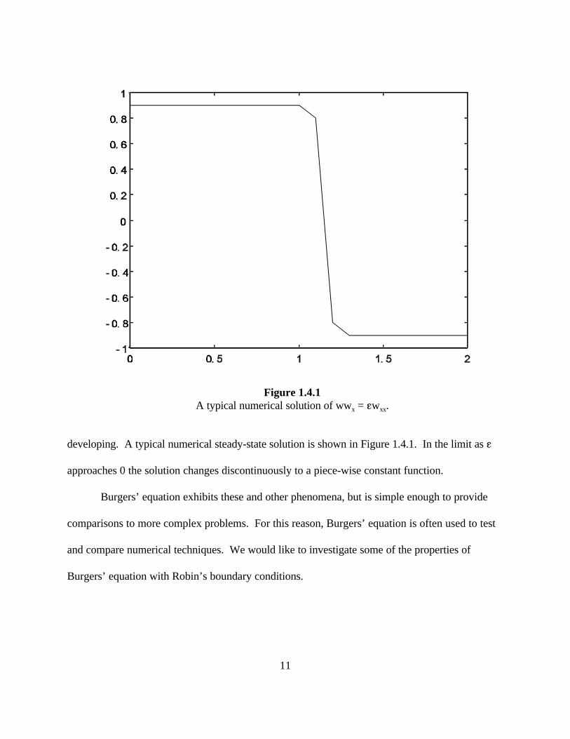
Figure 1.4.1A typical numerical solution of ww = gw .x xx

developing. A typical numerical steady-state solution is shown in Figure 1.4.1. In the limit as g

approaches 0 the solution changes discontinuously to a piece-wise constant function.

Burgers’ equation exhibits these and other phenomena, but is simple enough to provide

comparisons to more complex problems. For this reason, Burgers’ equation is often used to test

and compare numerical techniques. We would like to investigate some of the properties of

Burgers’ equation with Robin’s boundary conditions.

MwMt

(t,x) % w(t,x)MwMx

(t,x) ' g M2w

Mx 2(t,x)

MwMx

(t,0) ' 0;MwMx

(t,1) ' 0

w(0,x) ' w0(x).

MwMt

(t,x) %12MMx

(w 2(t,x)) ' g M2w

Mx 2(t,x).

12

1.5 Perspective

As mentioned in Section 1.4, Burgers’ equation was first studied by Bateman [10] and

then studied extensively by Burgers [11]. Fletcher [12] illustrates some of the dynamics and

difficulties of solving Burgers’ equation.

Pugh [1] compares the Galerkin finite element method and the Galerkin/Conservation

method in solving the homogeneous Burgers’ equation

with homogeneous Neumann boundary conditions on the interval [0,1]

with initial condition

In the conservation method, the homogeneous Burgers’ equation is written as

Pugh determined that N=16 elements provided adequate accuracy for his computations.

In several test cases, these computations gave solutions that converged to the exact solution as N

approaches infinity, as expected. Pugh discovered that the Galerkin/Conservation method

computed more quickly with less error than the Galerkin finite element method. In some

examples, the Galerkin/Conservation method converged to a solution when the Galerkin finite

w(t,0) ' 0; w(t,L) ' v(t).

13

element method diverged.

Byrnes, Gilliam, and Shubov [15] proved that for a sufficiently small initial condition, the

solution of the Burgers’ equation with Neumann boundary conditions must converge to a

constant as time approaches infinity. Burns et.al. [2] later showed that this was true for any initial

condition, provided the steady-state limit exists. Pugh, however, obtained non-constant steady-

state solutions for larger initial conditions and smaller g (R = 120, 240). We now know that thisE

is a purely numerical solution (see [2]).

Burgers’ equation has also provided a test case for research on the problem of active

control of fluid flows. Burns and Kang considered two linear regulator problems with Burgers’

equation. Both problems involved applying boundary conditions to finite spatial intervals. In the

first paper [16], they formulate a finite dimensional approximating system for the Burgers’

equation with homogeneous Dirichlet boundary conditions on the finite interval [0, L]. In the

second paper [17], the model was applied to the inhomogeneous Dirichlet case

In both papers, this nonlinear system of ordinary differential equations was solved using a fourth

order Runge-Kutta method [18].

Marrekchi [19] studied another boundary control problem using the Burgers’ equation

with homogeneous Neumann boundary conditions. The resulting system of N+2 ordinary

differential equations was solved with MATLAB using ODE45, which implements a fourth and

fifth order Runge-Kutta method. He found that on the interval [0,1] with R = 60, the solutionE

converged to a constant steady-state given the initial condition w (x) = -cos(Bx), but diverged for0

14

the initial condition w (x) = cos(Bx). Again, this is now known to be a purely numerical solution0

(see [2]).

Massa [20] is considering the boundary control problem of the Burgers’ equation with

Robin’s boundary conditions, using the same model and MATLAB code as this paper.

1.6 Goals

In order to investigate the Burgers’ equation with Robin’s boundary conditions, we need

to implement a numerical scheme to approximate the solution. We will be using a finite element

scheme employing piece-wise linear polynomial basis functions, which is developed in Chapter

two. We will investigate the accuracy of these schemes and determine which method is best

(Galerkin or Galerkin/Conservation) for Burgers’ equation with Robin’s boundary conditions.

We will also investigate the nature of the numerical solutions to the Burgers’ equation as

the Robin’s boundary conditions approach both the Dirichlet and the Neumann boundary

conditions. In particular, we want to know if solutions for the Robin’s boundary conditions

approach solutions resulting from the homogeneous Neumann boundary conditions as L and L1 2

approach infinity. A similar issue is considered when the Robin’s boundary conditions approach

the Dirichlet boundary conditions, i.e. as L and L approach zero. We would like to determine if1 2

this asymptotic method yields a realistic answer when the methods using only Dirichlet or

Neumann boundary conditions fail to.

MwMt

(t,x) % w(t,x)MwMx

(t,x) ' g M2w

Mx 2(t,x) % f(t,x)

61

L1

w(t,0) & 6 MwMx

(t,0) '61

L1

u1(t)62

L2

w(t,L) % 6 MwMx

(t,L) '62

L2

u2(t)

w(0,x) ' w0(x).

15

(2.1.1)

(2.1.2)

(2.1.3)

Chapter Two

The Finite Element Method

2.1 A Review of the Equations

We now turn our attention to the computations. We wish to numerically solve Burgers’

equation with Robin’s Boundary conditions on the interval [0,L]. In particular, consider Burgers’

equation

with boundary conditions

and initial condition

Again, it is helpful to think of w(t,x) as the temperature of the rod at time t and position x in our

model, described in Section 1.2. In this case, 6 is the thermal conductivity of the rod and g is the

thermal diffusivity of the rod. The constants 6 and 6 are the thermal conductivities of the left1 2

and right films of lengths L and L , respectively.1 2

mL

0

MwMt

(t,x)v(x)dx % mL

0w(t,x)

MwMx

(t,x)v(x)dx ' mL

0g M

2w

Mx 2(t,x)v(x)dx % m

L

0f(t,x)v(x)dx.

mL

0

MwMt

(t,x)v(x)dx'&mL

0w(t,x)

MwMx

(t,x)v(x)dx&mL

0g MwMx

(t,x)v'(x)dx%mL

0f(t,x)v(x)dx%g[

MwMx

(t,x)v(x)]L

0.

mL

0

MwMt

(t,x)v(x)dx ' &mL

0w(t,x)

MwMx

(t,x)v(x)dx & gmL

0

MwMx

(t,x)v'(x)dx % mL

0f(t,x)v(x)dx

%g62

6L2

u2(t)v(L) &g62

6L2

w(t,L)v(L) %g61

6L1

u1(t)v(0) &g61

6L1

w(t,0)v(0).

16

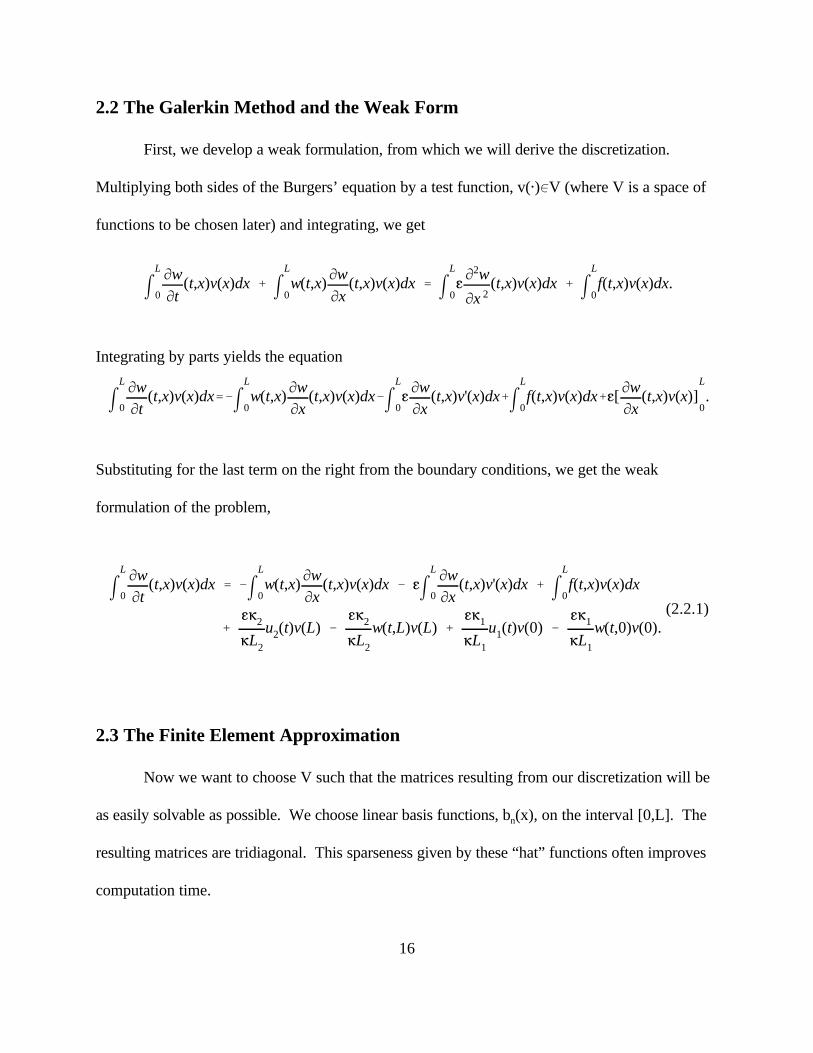
(2.2.1)

2.2 The Galerkin Method and the Weak Form

First, we develop a weak formulation, from which we will derive the discretization.

Multiplying both sides of the Burgers’ equation by a test function, v(")0V (where V is a space of

functions to be chosen later) and integrating, we get

Integrating by parts yields the equation

Substituting for the last term on the right from the boundary conditions, we get the weak

formulation of the problem,

2.3 The Finite Element Approximation

Now we want to choose V such that the matrices resulting from our discretization will be

as easily solvable as possible. We choose linear basis functions, b (x), on the interval [0,L]. Then

resulting matrices are tridiagonal. This sparseness given by these “hat” functions often improves

computation time.

b0(x)'x1&x

hfor x0#x#x1

0 elsewhere

bN%1(x)'x&xN

hfor xN#x#xN%1

0 elsewhere

bi(x)'

x&xi&1

hfor xi&1#x#xi

xi&x

hfor xi#x#xi%1

0 elsewhere

w N(t,x) ' jN%1

i'0di(t)bi(x),

17

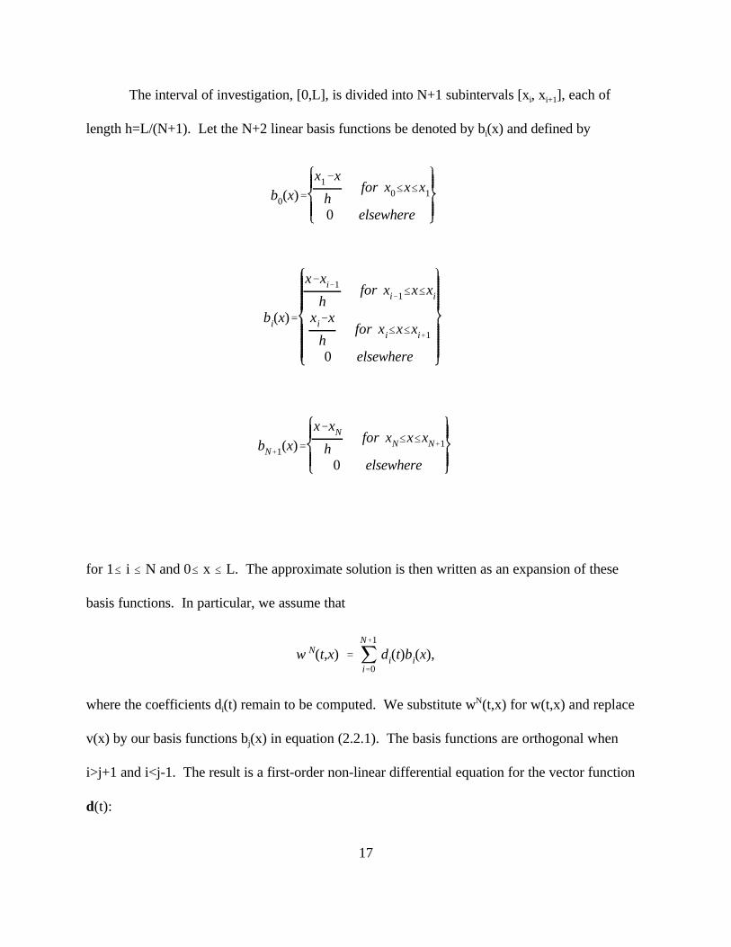
The interval of investigation, [0,L], is divided into N+1 subintervals [x , x ], each ofi i+1

length h=L/(N+1). Let the N+2 linear basis functions be denoted by b (x) and defined by i

for 1# i # N and 0# x # L. The approximate solution is then written as an expansion of these

basis functions. In particular, we assume that

where the coefficients d (t) remain to be computed. We substitute w (t,x) for w(t,x) and replaceiN

v(x) by our basis functions b (x) in equation (2.2.1). The basis functions are orthogonal whenj

i>j+1 and i<j-1. The result is a first-order non-linear differential equation for the vector function

d(t):

mL

0 jN%1

i'0

0di(t)bi(x)bj(x)dx ' &mL

0 jN%1

i'0di(t)bi(x)j

N%1

k'0dk(t)bk'(x)bj(x)dx&gm

L

0 jN%1

i'0di(t)bi'(x)bj'(x)dx

% mL

0f(x,t)bj(x)dx &

g62

6L2jN%1

i'0di(t)bi(L)bj(L)%

g62

6L2

u2(t)bj(L)

%g61

6L1

u1(t)bj(0)&g61

6L1jN%1

i'0di(t)bi(0)bj(0).

00d(t) '

0d0(t)

0d1(t)

!

0dN%1(t) (N%2)×1

mi,j ' mL

0bi(x)bj(x)dx.

18

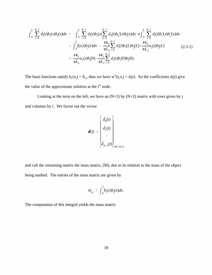
(2.3.1)

The basis functions satisfy b (x ) = * , thus we have w (t,x ) = d (t). So the coefficients d (t) givei j i j i i iN

the value of the approximate solution at the i node.th

Looking at the term on the left, we have an (N+2) by (N+2) matrix with rows given by j

and columns by i. We factor out the vector

and call the remaining matrix the mass matrix, [M], due to its relation to the mass of the object

being studied. The entries of the mass matrix are given by

The computation of this integral yields the mass matrix

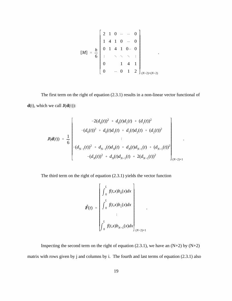
[M] 'h6

2 1 0 þ þ 0

1 4 1 0 þ 0

0 1 4 1 0þ 0

! " " " !

0 1 4 1

0 þ 0 1 2 (N%2)×(N%2)

.

J(d(t)) '16

&2(d0(t))2 % d0(t)d1(t) % (d1(t))

2

&(d0(t))2 % d0(t)d1(t) % d1(t)d2(t) % (d2(t))

2

!

&(dN&1(t))2 % dN&1(t)dN(t) % dN(t)dN%1(t) % (dN%1(t))

2

&(dN(t))2 % dN(t)dN%1(t) % 2(dN%1(t))2

(N%2)×1

.

F̂(t) '

mL

0f(t,x)b0(x)dx

mL

0f(t,x)b1(x)dx

!

mL

0f(t,x)bN%1(x)dx

(N%2)×1

.

19

The first term on the right of equation (2.3.1) results in a non-linear vector functional of

d(t), which we call J(d(t)):

The third term on the right of equation (2.3.1) yields the vector function

Inspecting the second term on the right of equation (2.3.1), we have an (N+2) by (N+2)

matrix with rows given by j and columns by i. The fourth and last terms of equation (2.3.1) also

d(t) '

d0(t)

d1(t)

!

dN%1(t) (N%2)×1

ki,j ' mL

0bi'(x)bj'(x)dx

[K] '1h

&1&h61

6L1

1 0 þ þ 0

1 &2 1 0 þ 0

0 1 &2 1 0þ 0

! " " " !

0 1 &2 1

0 þ 0 1 &1&h62

6L2 (N%2)×(N%2)

.

20

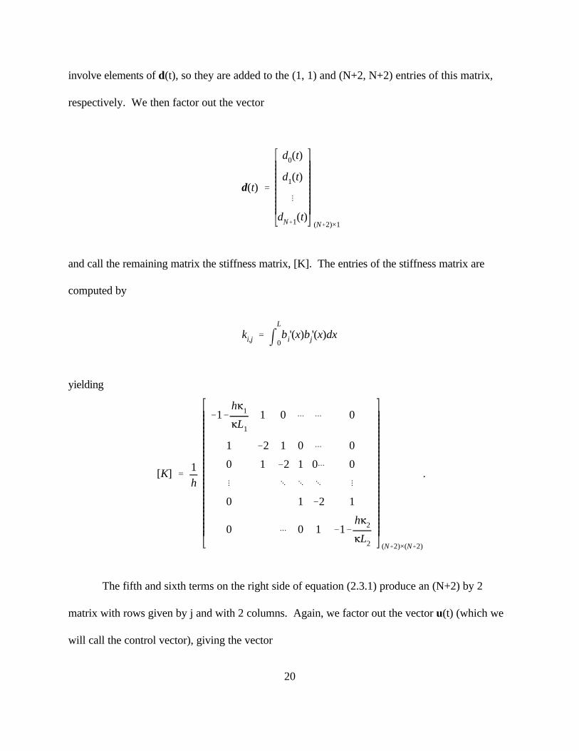
involve elements of d(t), so they are added to the (1, 1) and (N+2, N+2) entries of this matrix,

respectively. We then factor out the vector

and call the remaining matrix the stiffness matrix, [K]. The entries of the stiffness matrix are

computed by

yielding

The fifth and sixth terms on the right side of equation (2.3.1) produce an (N+2) by 2

matrix with rows given by j and with 2 columns. Again, we factor out the vector u(t) (which we

will call the control vector), giving the vector

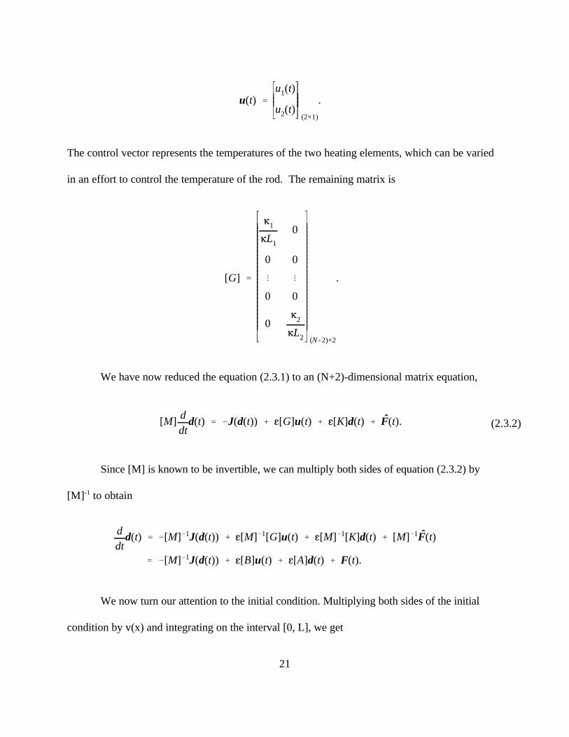
u(t) '

u1(t)

u2(t) (2×1)

.

[G] '

61

6L1

0

0 0

! !

0 0

062

6L2 (N%2)×2

.

[M]ddt

d(t) ' &J(d(t)) % g[G]u(t) % g[K]d(t) % F̂(t).

ddt

d(t) ' &[M]&1J(d(t)) % g[M]&1[G]u(t) % g[M]&1[K]d(t) % [M]&1F̂(t)

' &[M]&1J(d(t)) % g[B]u(t) % g[A]d(t) % F(t).

21

(2.3.2)

The control vector represents the temperatures of the two heating elements, which can be varied

in an effort to control the temperature of the rod. The remaining matrix is

We have now reduced the equation (2.3.1) to an (N+2)-dimensional matrix equation,

Since [M] is known to be invertible, we can multiply both sides of equation (2.3.2) by

[M] to obtain-1

We now turn our attention to the initial condition. Multiplying both sides of the initial

condition by v(x) and integrating on the interval [0, L], we get

mL

0w(0,x)v(x)dx ' m

L

0w0(x)v(x)dx.

mL

0 jN%1

i'0di(0)bi(x)bj(x)dx ' m

L

0w0(x)bj(x)dx,

d(0) '

d0(0)

d1(0)

!

dN%1(0)(N%2)×1

w N0 '

mL

0w0(x)b0(x)dx

mL

0w0(x)b1(x)dx

!

mL

0w0(x)bN%1(x)dx

(N%2)×1

.

22

(2.3.3)

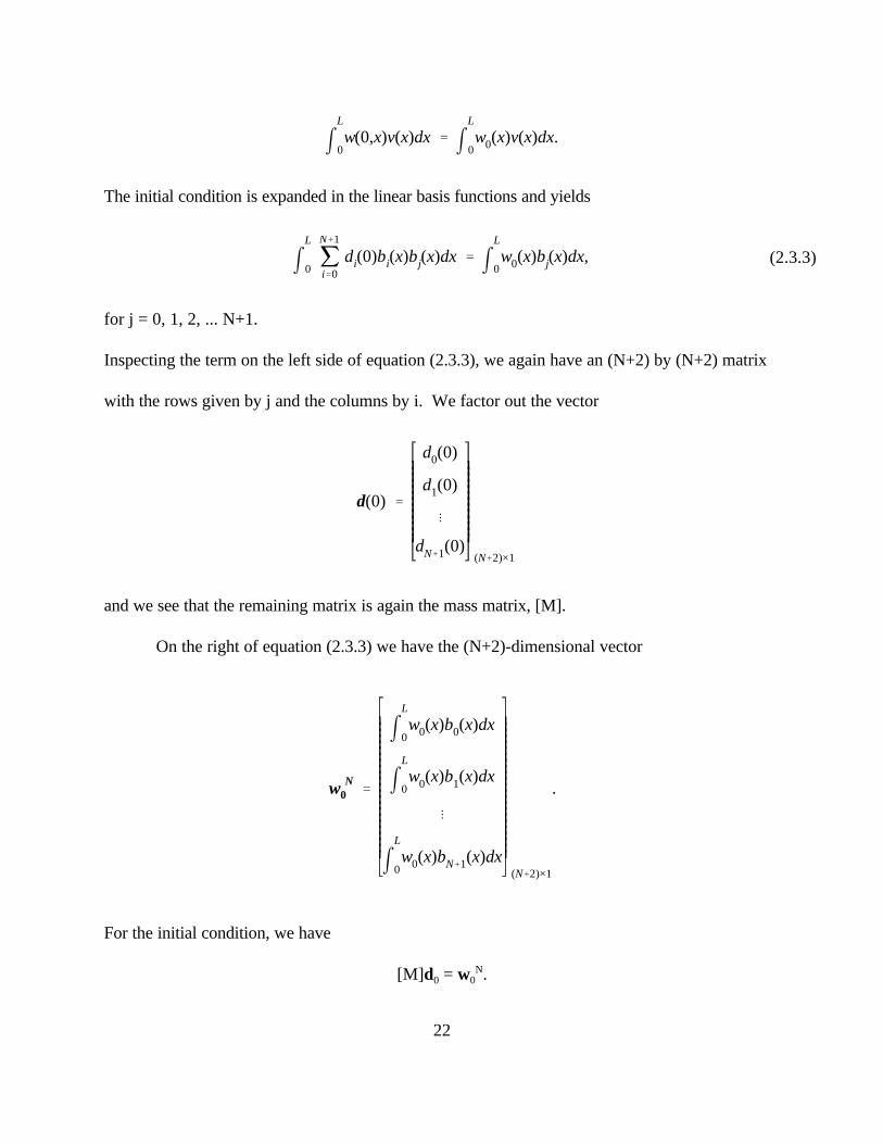
The initial condition is expanded in the linear basis functions and yields

for j = 0, 1, 2, ... N+1.

Inspecting the term on the left side of equation (2.3.3), we again have an (N+2) by (N+2) matrix

with the rows given by j and the columns by i. We factor out the vector

and we see that the remaining matrix is again the mass matrix, [M].

On the right of equation (2.3.3) we have the (N+2)-dimensional vector

For the initial condition, we have

[M]d = w .0 0N

00d(t) ' &[M]&1J(d(t)) % g[A]d(t) % g[B]u(t) % F(t)

d0 ' [M]&1wN0 .

MwMt

(t,x) %12MMx

(w 2(t,x)) ' g M2w

Mx 2(t,x) % f(t,x).

23

(2.3.4)

(2.3.5)

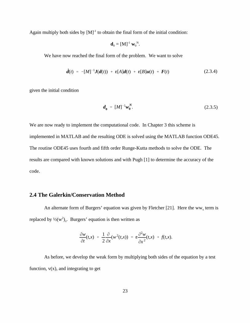
Again multiply both sides by [M] to obtain the final form of the initial condition:-1

d = [M] w .0 0-1 N

We have now reached the final form of the problem. We want to solve

given the initial condition

We are now ready to implement the computational code. In Chapter 3 this scheme is

implemented in MATLAB and the resulting ODE is solved using the MATLAB function ODE45.

The routine ODE45 uses fourth and fifth order Runge-Kutta methods to solve the ODE. The

results are compared with known solutions and with Pugh [1] to determine the accuracy of the

code.

2.4 The Galerkin/Conservation Method

An alternate form of Burgers’ equation was given by Fletcher [21]. Here the ww term isx

replaced by ½(w ) . Burgers’ equation is then written as2x

As before, we develop the weak form by multiplying both sides of the equation by a test

function, v(x), and integrating to get

mL

0

MwMt

(t,x)v(x)dx % mL

0

12MMx

(w 2(t,x))v(x)dx ' mL

0g M

2w

Mx 2(t,x)v(x)dx % m

L

0f(t,x)v(x)dx.

mL

0

MwMt

(t,x)v(x)dx ' &mL

0

12

MMx

[w 2(t,x)]v(x)dx & gmL

0

MwMx

(t,x)v'(x)dx % mL

0f(t,x)v(x)dx

%g62

6L2

u2(t)v(L) &g62

6L2

w(t,L)v(L) %g61

6L1

u1(t)v(0) &g61

6L1

w(t,0)v(0).

[w N(t,x)]2 ' jN%1

i'0

(di(t))2hi(x).

mL

0 jN%1

i'0

0di(t)bi(x)bj(x)dx ' &mL

0

12j

N%1

i'0

(di(t))2b0i'(x)bj(x)dx & gm

L

0 jN%1

i'0

di(t)bi'(x)bj'(x)dx

% mL

0f(x,t)bj(x)dx &

g62

6L2jN%1

i'0

di(t)bi(L)bj(L)%g62

6L2

u2(t)bj(L)

%g61

6L1

u1(t)bj(0)&g61

6L1jN%1

i'0

di(t)bi(0)bj(0).

24

(2.4.1)

We integrate the second order term by parts to get a weak form

Again we choose the space of linear polynomials for our test space, using the basis

functions given in Section 2.3. In addition to the trial solution w (t,x) given in Section 2.3, weN

now need to postulate a trial solution for [w(t,x)] ,2

Letting v(x)=b (x) and substituting into equation (2.4.1) as before, we get a non-linear differentialj

equation for the vector function d(t),

This then reduces to

[M]ddt

d(t) ' &JC(d(t)) % g[G]u(t) % g[K]d(t) % F̂(t)

JC(d(t)) '14

(d1(t))2 & (d0(t))

2

(d2(t))2 & (d0(t))

2

(d3(t))2 & (d1(t))

2

!

(dN%1(t))2 & (dN&1(t))

2

(dN%1(t))2 & (dN(t))2

(N%2)×1

.

00d(t) ' &[M]&1JC(d(t)) % g[A]d(t) % g[B]u(t) % F(t)

d0 ' [M]&1 wN0 .

25

(2.4.2)

(2.4.3)

(2.4.4)

through the process shown in Section 2.3. This equation is equal to equation (2.3.2), except that

J(d(t)) has been replaced by J (d(t)):C

Finally, we multiply both sides of equation (2.4.2) by [M ]. The initial condition is transformed in-1

the same manner as in Section 2.3, giving us the final system to be solved. We want to solve


This system is solved in Chapter 3 using the MATLAB function ODE45. The results are

compared with the results from the Galerkin finite element method of Section 2.3.

MwMt

(t,x) % w(t,x)MwMx

(t,x) ' g M2w

Mx 2(t,x) % f(t,x)

61

L1

w(t,0) % 6 MwMx

(t,0) '61

L1

u1(t);62

L2

w(t,L) % 6 MwMx

(t,L) '62

L2

u2(t)

w(x,0) ' w0(x).

00d(t) % [M]&1J(d(t)) ' g[A]d(t) % g[B]u(t) % F(t)

d0 ' [M]&1wN0 .

26

(3.1.1)

Chapter Three

NUMERICAL RESULTS

3.1 Setting Up the Problem

Consider the Burgers’ equation

with Robin’s boundary conditions

and initial condition w (x)0

We are interested in computing approximate solutions of this problem.

The Galerkin finite element model was described in Chapter 2 and results in a system of

ordinary differential equations:

Here J(d(t)) changes to J (d(t)) when the Galerkin/Conservation method is used, as shown inC

Section 2.4.

Error (t) ' [ mL

0(w N(t,x)&w(t,x))2dx ]1/2.

27

This problem is set up in MATLAB and solved using the ODE45 ordinary differential

equation solver. Most of the examples presented in this paper employ numerical approximation

schemes using N=16 elements. This is the most cost-effective number of elements, as shown in

Section 3.2. This partitions the x-interval, [0,L], into N+1=17 subintervals of uniform length.

The result is N+2=18 nodes, making (3.1.1) a system of 18 ordinary differential equations.

In nearly all of the examples in this paper, we use the Galerkin/Conservation method due

to the increased efficiency afforded by it over the Galerkin method. This choice is supported in

Sections 3.2 and 3.3, as well as by Pugh [1].

In some examples, we have an a priori knowledge of the exact solution. In this case, we

measure the numerical error introduced by the two approximating schemes, by calculating the L2

error at time t given by

This integral is computed using a three-point Guass quadrature scheme. This scheme evaluates

(w (t,x)-w(t,x)) at three points in each subinterval, weighting each point differently. On theN 2

interval [-1,1], these points are x=-0.77459667, 0, 0.77459667 with weights 0.55555556,

0.88888889, and 0.55555556, respectively. These points and weights are chosen so as to

optimize the accuracy of the numerical integration. The three-point Gauss quadrature scheme can

integrate polynomials of order (2n-1)=5 exactly [18]. This is more than enough accuracy for

computing the error of our numerical solutions, which are composed of piece-wise polynomials of

order one.

The error is also shown graphically by computing w (t,x) and w(t,x) at five evenly-spacedN

f(t,x) ' wt(t,x) % w(t,x)wx(t,x) & gwxx(t,x),

u1(t) ' w(t,0) &6L1

61

wx(t,0) and u2(t) ' w(t,L) %6L2

62

wx(t,L).

28

points in each subinterval. The exact solution and the difference w (t,x) - w(t,x) are then plottedN

at these points for comparison.

3.2 A Comparison to Known Solutions

In this section, we compare two methods of computation on two problems.The goal is to

verify that the numerical schemes are returning the correct answer. We also want to determine

which method and how many elements to use. The Galerkin method is compared to the

Galerkin/Conservation method for N=4, 8, 16, and 32 elements. We conclude that the Galerkin/

Conservation method employing N=16 elements is the best choice for our computations.

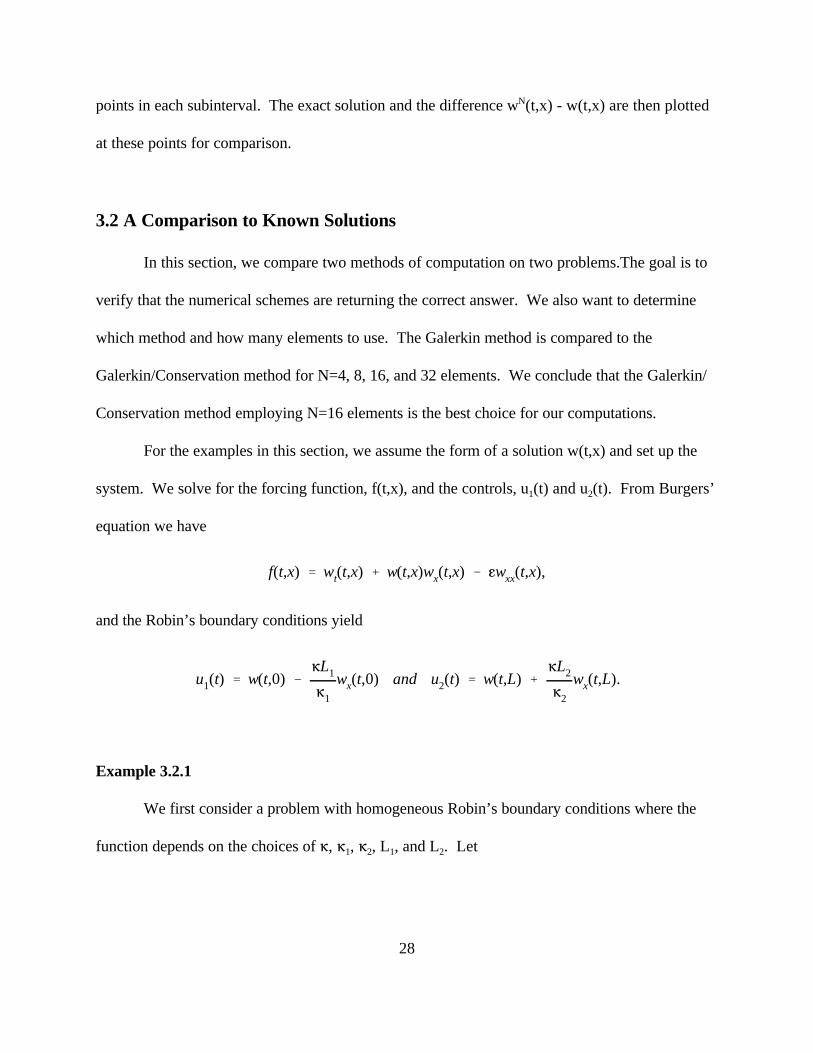
For the examples in this section, we assume the form of a solution w(t,x) and set up the

system. We solve for the forcing function, f(t,x), and the controls, u (t) and u (t). From Burgers’1 2

equation we have

and the Robin’s boundary conditions yield

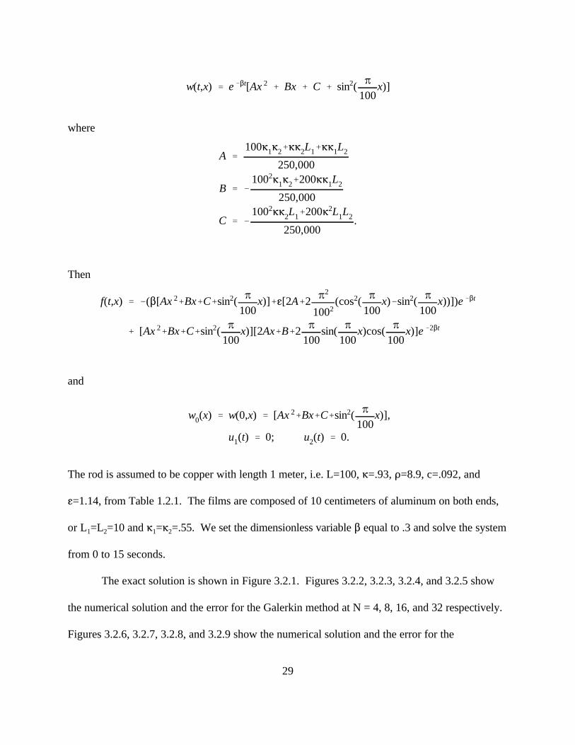
Example 3.2.1

We first consider a problem with homogeneous Robin’s boundary conditions where the

function depends on the choices of 6, 6 , 6 , L , and L . Let 1 2 1 2

w(t,x) ' e &$t[Ax 2 % Bx % C % sin2(B

100x)]

A '1006162%662L1%661L2

250,000

B ' &10026162%200661L2

250,000

C ' &1002662L1%20062L1L2

250,000.

f(t,x) ' &($[Ax 2%Bx%C%sin2(B

100x)]%g[2A%2

B2

1002(cos2(

B100

x)&sin2(B

100x))])e &$t

% [Ax 2%Bx%C%sin2(B

100x)][2Ax%B%2

B100

sin(B

100x)cos(

B100

x)]e &2$t

w0(x) ' w(0,x) ' [Ax 2%Bx%C%sin2( B100

x)],

u1(t) ' 0; u2(t) ' 0.

29

where

Then

and

The rod is assumed to be copper with length 1 meter, i.e. L=100, 6=.93, D=8.9, c=.092, and

g=1.14, from Table 1.2.1. The films are composed of 10 centimeters of aluminum on both ends,

or L =L =10 and 6 =6 =.55. We set the dimensionless variable $ equal to .3 and solve the system1 2 1 2

from 0 to 15 seconds.

The exact solution is shown in Figure 3.2.1. Figures 3.2.2, 3.2.3, 3.2.4, and 3.2.5 show

the numerical solution and the error for the Galerkin method at N = 4, 8, 16, and 32 respectively.

Figures 3.2.6, 3.2.7, 3.2.8, and 3.2.9 show the numerical solution and the error for the

30

Galerkin/Conservation method at N = 4, 8, 16, and 32 respectively.

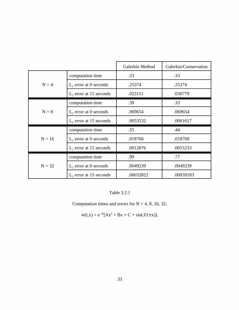
Table 3.2.1 compares the errors and computational time on a Pentium 133 for the

Galerkin and Galerkin/Conservation methods using N= 4, 8, 16, and 32. At the initial time, t =0,i

the errors for the Galerkin and the Galerkin/Conservation methods will always be equal due to the

fact that d = [M ] w , which has no dependence on the nonlinear term. The error at the initial0-1

0N

time is dependent only on the spatial grid size, i.e. N. The error decreases with time because the

solution decreases with time.

Comparing the errors at the final time for N = 4, 8, 16, and 32, we see that our numerical

solutions are converging to the exact solution at better than the expected rate (1/N ) for both the½

Galerkin and the Galerkin/Conservation methods. This is consistent with the finite element theory

found in [21]. The errors for the Galerkin method are slightly smaller than the errors for the

Galerkin/Conservation method. However, the Galerkin/Conservation method is computationally

faster than the Galerkin method, especially as N increases to 16 and 32. Since the

Galerkin/Conservation method is faster with only a small error difference, we will use it for all of

the computations in Sections 3.3 and 3.4.

Comparing the errors at the initial and final time for N = 4, 8, 16, and 32, we see that

sufficient accuracy is achieved at N = 16 elements. This is supported graphically in

Figures 3.2.4 and 3.2.8.

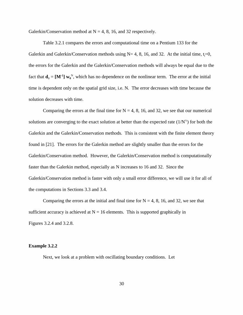
Example 3.2.2

Next, we look at a problem with oscillating boundary conditions. Let

w(t,x) '(100&x)2

1002sin("t) %

x 2

1002cos($t).

f(t,x) ' " (100&x)2

1002cos("t)&$ x 2

1002sin($t)&2

(100&x)3

1004sin2("t)%2

x 3

1004cos2($t)

%2

1004(2x 3&300x 2%1002x)sin("t)cos($t)& 2g

1002(sin("t)%cos($t))

w0(x) ' w(0,x) 'x 2

1002,

u1(t) ' (1%26L1

10061

)sin("t); u2(t) ' (1%26L2

10062

)cos($t).

31

Then

and

One thing we notice about this problem is that at the left end w(t,x)=sin("t) and at the right end

w(t,x)=cos($t). The oscillations of the boundaries can be made as slow or fast as desired by

varying " and $.

Again, we let the rod be composed of one meter of copper and the films be composed of

10 centimeters of aluminum on both ends. We set the dimensionless variables " and $ equal to

1.5B and .5B respectively. We then solve the system from zero to ten seconds.

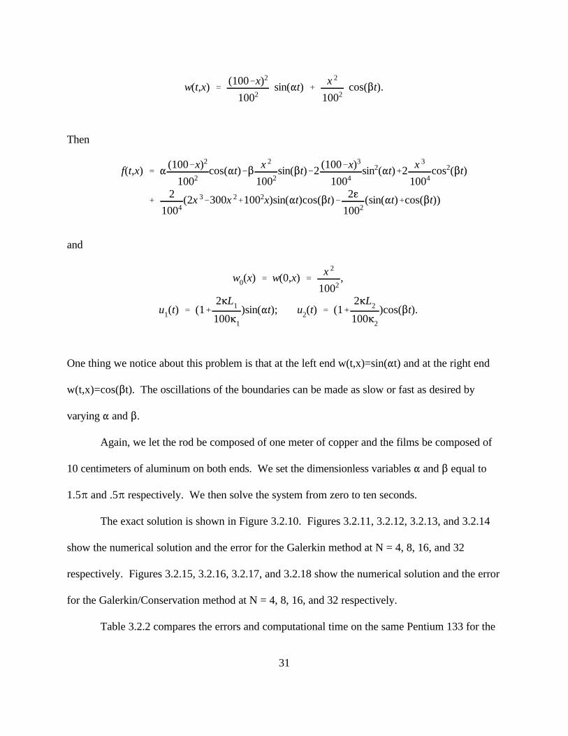
The exact solution is shown in Figure 3.2.10. Figures 3.2.11, 3.2.12, 3.2.13, and 3.2.14

show the numerical solution and the error for the Galerkin method at N = 4, 8, 16, and 32

respectively. Figures 3.2.15, 3.2.16, 3.2.17, and 3.2.18 show the numerical solution and the error

for the Galerkin/Conservation method at N = 4, 8, 16, and 32 respectively.

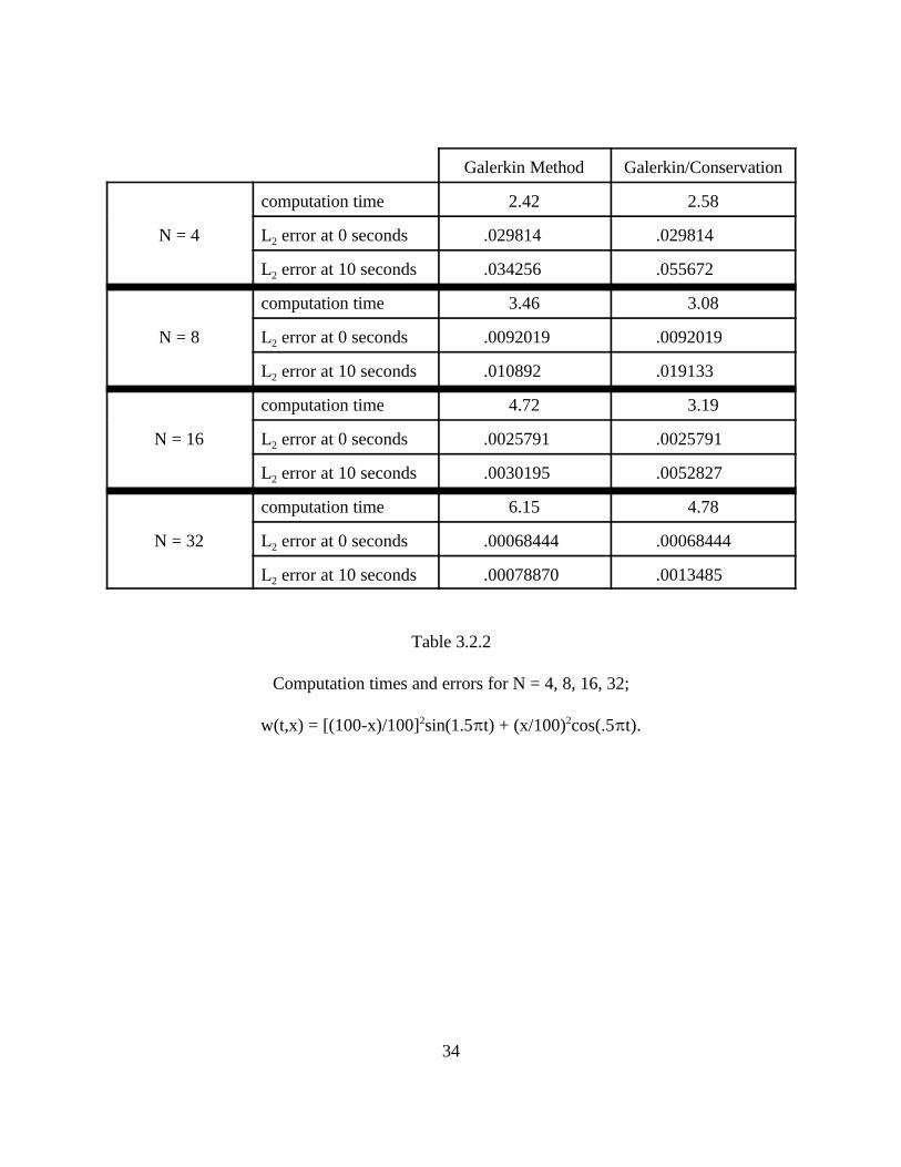
Table 3.2.2 compares the errors and computational time on the same Pentium 133 for the

32

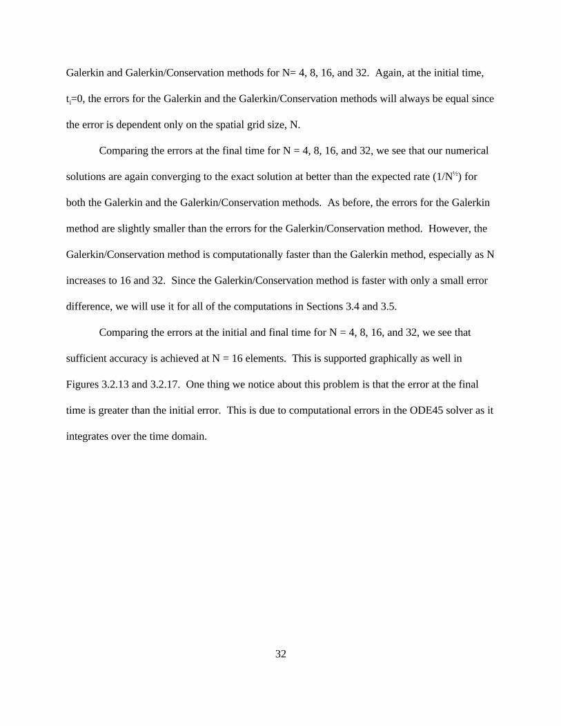
Galerkin and Galerkin/Conservation methods for N= 4, 8, 16, and 32. Again, at the initial time,

t =0, the errors for the Galerkin and the Galerkin/Conservation methods will always be equal sincei

the error is dependent only on the spatial grid size, N.

Comparing the errors at the final time for N = 4, 8, 16, and 32, we see that our numerical

solutions are again converging to the exact solution at better than the expected rate (1/N ) for½

both the Galerkin and the Galerkin/Conservation methods. As before, the errors for the Galerkin

method are slightly smaller than the errors for the Galerkin/Conservation method. However, the

Galerkin/Conservation method is computationally faster than the Galerkin method, especially as N

increases to 16 and 32. Since the Galerkin/Conservation method is faster with only a small error

difference, we will use it for all of the computations in Sections 3.4 and 3.5.

Comparing the errors at the initial and final time for N = 4, 8, 16, and 32, we see that

sufficient accuracy is achieved at N = 16 elements. This is supported graphically as well in

Figures 3.2.13 and 3.2.17. One thing we notice about this problem is that the error at the final

time is greater than the initial error. This is due to computational errors in the ODE45 solver as it

integrates over the time domain.

33

Galerkin Method Galerkin/Conservation

N = 4 L error at 0 seconds .25374 .25374

computation time .33 .33

2

L error at 15 seconds .023151 .0307792



2




2




2


Table 3.2.1

Computation times and errors for N = 4, 8, 16, 32;

w(t,x) = e [Ax + Bx + C + sin(.01Bx)].-.3t 2

34

Galerkin Method Galerkin/Conservation


computation time 2.42 2.58

2

L error at 10 seconds .034256 .055672 2



2




2




2


Table 3.2.2

Computation times and errors for N = 4, 8, 16, 32;

w(t,x) = [(100-x)/100] sin(1.5Bt) + (x/100) cos(.5Bt).2 2

MwMt

(t,x) % w(t,x)MwMx

(t,x) '1

RE

M2w

Mx 2(t,x)

MwMx

(t,0) 'MwMx

(t,L) ' 0

w(0,x) ' w0(x).

53

3.3 A Comparison to Previous Work

In this section, we compare our solutions to the results obtained by Pugh [1] for the

homogeneous Burgers’ equation with homogeneous Neumann boundary conditions. Here f(t,x) is

set equal to zero producing the homogeneous Burgers’ equation. The homogeneous Neumann

boundary conditions are obtained by setting 6 and 6 equal to zero. This is equivalent to using1 2

two films both made of a perfect insulator. The other constants are treated as dimensionless with

6=1 and g=1/R . We want to solveE

subject to the homogeneous Neumann boundary conditions


The interval of interest we pick to be x 0 [0,1], matching Pugh.

Example 3.3.1

In this example we compare our solution to those obtained by Pugh for

w (x)=(1/16)cos(Bx). Figures 3.3.1, 3.3.2 and 3.3.3 show the results for R = 60, 120, and 2400 E

respectively. Comparing with pages 47, 48, and 49 of Pugh [1], we see that our results are in

very good agreement with his results. We also see that the Galerkin and Galerkin/Conservation

54

method give similar results in all three cases. This supports our choice of the

Galerkin/Conservation method for our computations due to its faster computation.

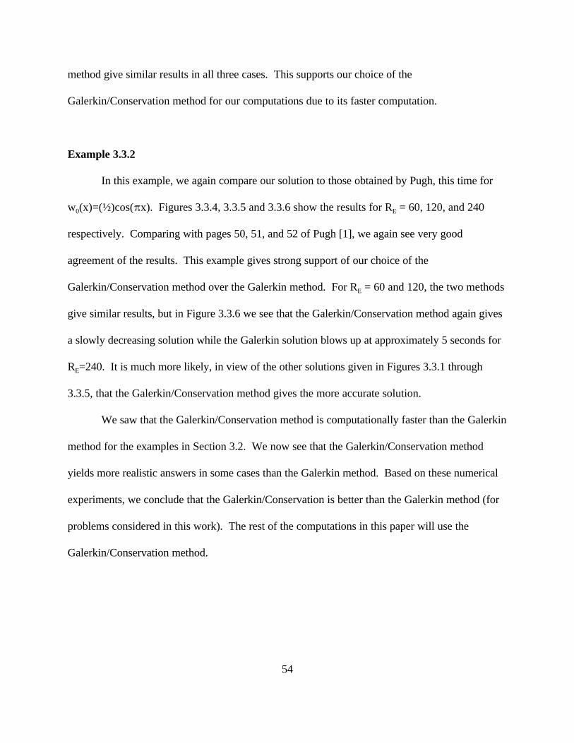
Example 3.3.2

In this example, we again compare our solution to those obtained by Pugh, this time for

w (x)=(½)cos(Bx). Figures 3.3.4, 3.3.5 and 3.3.6 show the results for R = 60, 120, and 2400 E

respectively. Comparing with pages 50, 51, and 52 of Pugh [1], we again see very good

agreement of the results. This example gives strong support of our choice of the

Galerkin/Conservation method over the Galerkin method. For R = 60 and 120, the two methodsE

give similar results, but in Figure 3.3.6 we see that the Galerkin/Conservation method again gives

a slowly decreasing solution while the Galerkin solution blows up at approximately 5 seconds for

R =240. It is much more likely, in view of the other solutions given in Figures 3.3.1 throughE

3.3.5, that the Galerkin/Conservation method gives the more accurate solution.

We saw that the Galerkin/Conservation method is computationally faster than the Galerkin

method for the examples in Section 3.2. We now see that the Galerkin/Conservation method

yields more realistic answers in some cases than the Galerkin method. Based on these numerical

experiments, we conclude that the Galerkin/Conservation is better than the Galerkin method (for

problems considered in this work). The rest of the computations in this paper will use the

Galerkin/Conservation method.

61

L1

w(t,0)&6 MwMx

(t,0)'61

L1

u1(t);62

L2

w(t,L)%6 MwMx

(t,L)'62

L2

u2(t).

w(t,0)'u1(t); w(t,L)'u2(t).

61

3.4 Results Approaching Dirichlet Boundary Conditions

In this section, we examine the behavior of the solutions as the Robin’s boundary

conditions approach the Dirichlet boundary conditions. As noted in Section 1.3, the Robin’s

boundary conditions are

The Dirichlet boundary conditions are given by

It is easily seen that the Robin’s boundary conditions approach the Dirichlet boundary conditions

when 6 approachs zero. This can also be implemented by letting 6 and 6 approach infinity or by1 2

letting L and L approach zero. If we let 6 approach zero, we are assuming an increase in the1 2

insulating properties of the rod. This implies the existence of a perfect insulator in the limit (a

common assumption). If we let 6 and 6 approach infinity, we require a perfect thermal1 2

conductor in the limit. However, letting L and L approach infinity or zero is mathematically1 2

equivalent and easily implemented in the code. Thus, we use L and L as parameters to vary. As1 2

we will see, for a rod one meter long, L and L need only be as small as one millimeter in some1 2

cases to achieve results similar to what is expected for “exact” Dirichlet boundary conditions.

Although the Galerkin and Galerkin/Conservation methods give similar solutions in many

cases, we have concluded that the Galerkin/Conservation method is more likely to capture the

actual evolution of the solution and that this approximation is generally faster to compute. We

therefore use the Galerkin/Conservation method for the rest of the computations in this and the

62

next section.

Example 3.4.1

In this example, we consider a one meter long rod composed of iron with copper films on

both ends, i.e. L=100, 6=.124, D=7.3, c=.099, g=.172, and 6 =6 =.93 from Table 1.2.1. We1 2

choose w (x) = (½)cos(.01Bx) for the initial condition and set the controls to zero, i.e.0

u (t)=u (t)=0. Figure 3.4.1 shows the long term evolution of the solution for L =L = 10. This1 2 1 2

solution is representative of the long term evolution for the problems in this example. The

solution eventually reduces to near zero, as expected. We are interested in the short term

evolution of the solutions, however. True Dirichlet boundary conditions would force the

solutions to zero at the ends almost immediately. Figures 3.4.2, 3.4.3, 3.4.4, and 3.4.5 show the

results for L =L = 10, 1, 0.1, and 0.01 respectively. 1 2

We see that the solutions are approaching what we would expect the solution to look like

for true Dirichlet boundary conditions. When L =L = 0.01, the solution is forced to zero almost1 2

immediately, as expected. We see that, in this case, film lengths of 0.01cm are small enough to

yield qualitatively the Dirichlet results. However, the film lengths are not the only factor. We

also need to be concerned with 6, 6 , and 6 , since it is the ratios of 6 /L and 6 /L to 6 that1 2 1 1 2 2

determines how close we are to the Dirichlet boundary conditions. In this case, (6 /L )/6 =1 1

(6 /L )/6 = 750 is sufficient to produce qualitatively the Dirichlet results. 2 2

Example 3.4.2

In this example, we consider a one meter long rod now composed of aluminum with silver

63

films on both ends, i.e. L=100, 6=.55, D=2.7, c=.217, g=.94, and 6 =6 =1. Now we choose w (x)1 2 0

= .3sin(.01Bx) for the initial condition and again set the controls to zero, i.e. u (t)=u (t)=0. Figure1 2

3.4.6 shows the long term evolution of the solution for L =L = 10. This solution is representative1 2

of the long term evolution for the problems in this example. The solutions eventually reduce to

near zero, as expected. Again we are interested in the short term evolution of the solution,

however. True Dirichlet boundary conditions would force the solution to remain at zero at the

ends for all time. Figures 3.4.7, 3.4.8, and 3.4.9 show the results for L =L = 10, 1, and 0.11 2

respectively.

We see that the solutions are approaching what we would expect the solution to look like

for true Dirichlet boundary conditions. When L =L = 0.1, the solution remains at zero at both1 2

ends, as expected. We see that, in this example, film lengths of 0.1cm are small enough to yield

qualitatively the Dirichlet results. In this case, (6 /L )/6 = (6 /L )/6 is approximately 18.1 1 2 2

61

L1

w(t,0)&6 MwMx

(t,0)'61

L1

u1(t);62

L2

w(t,L)%6 MwMx

(t,L)'62

L2

u2(t)

6 MwMx

(t,0)'0; 6 MwMx

(t,L)'0.

73

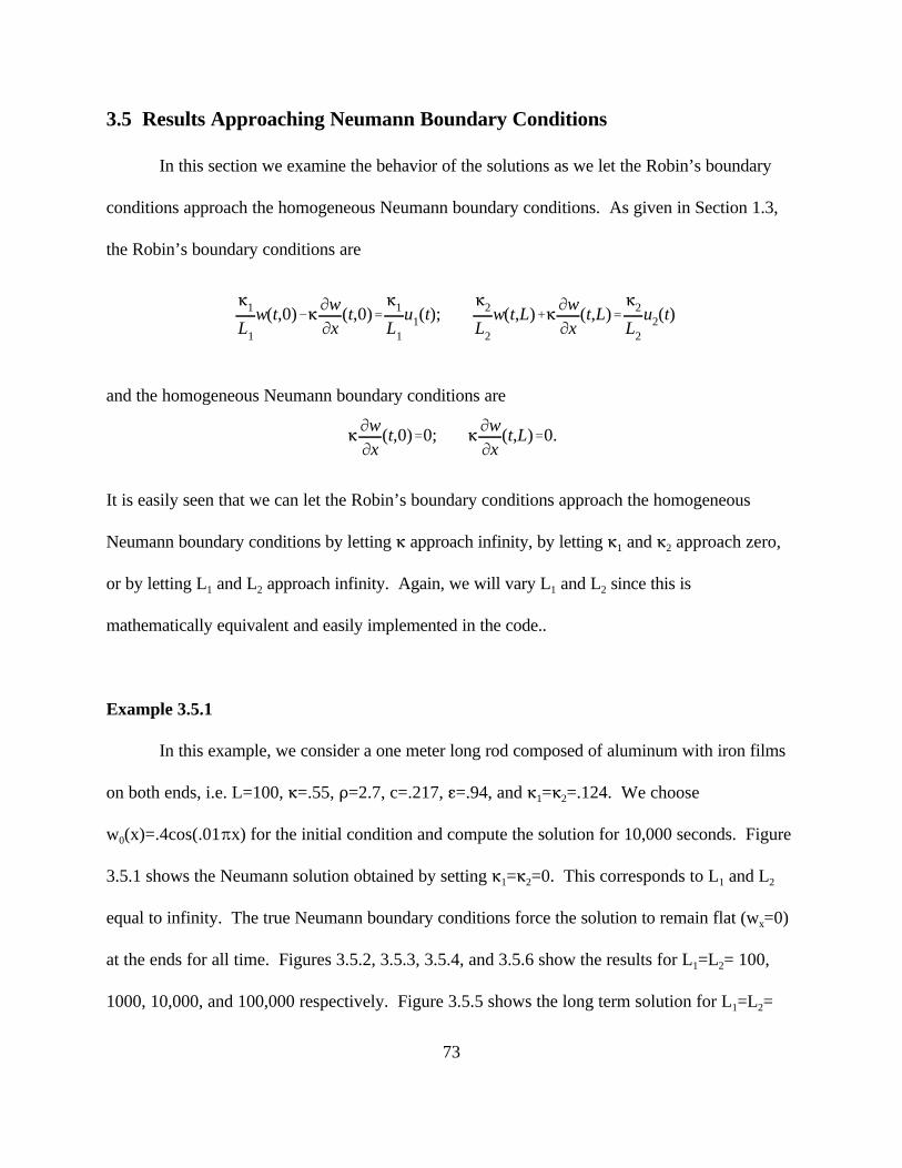
3.5 Results Approaching Neumann Boundary Conditions

In this section we examine the behavior of the solutions as we let the Robin’s boundary

conditions approach the homogeneous Neumann boundary conditions. As given in Section 1.3,

the Robin’s boundary conditions are

and the homogeneous Neumann boundary conditions are

It is easily seen that we can let the Robin’s boundary conditions approach the homogeneous

Neumann boundary conditions by letting 6 approach infinity, by letting 6 and 6 approach zero,1 2

or by letting L and L approach infinity. Again, we will vary L and L since this is1 2 1 2

mathematically equivalent and easily implemented in the code..

Example 3.5.1

In this example, we consider a one meter long rod composed of aluminum with iron films

on both ends, i.e. L=100, 6=.55, D=2.7, c=.217, g=.94, and 6 =6 =.124. We choose1 2

w (x)=.4cos(.01Bx) for the initial condition and compute the solution for 10,000 seconds. Figure0

3.5.1 shows the Neumann solution obtained by setting 6 =6 =0. This corresponds to L and L1 2 1 2

equal to infinity. The true Neumann boundary conditions force the solution to remain flat (w =0)x

at the ends for all time. Figures 3.5.2, 3.5.3, 3.5.4, and 3.5.6 show the results for L =L = 100,1 2

1000, 10,000, and 100,000 respectively. Figure 3.5.5 shows the long term solution for L =L =1 2

74

10,000. It appears that the solution reaches a non-zero constant steady state.after approximately

170,000 seconds.

We see that the solutions are approaching the solution for Neumann boundary conditions

as L and L approach zero. However, it appears that the solutions using the Robin’s boundary1 2

conditions will eventually reach zero, while the Neumann solution appears to remain nonzero

indefinitely. We see that, in this example, L = L = 100,000 is large enough to yield1 2

approximately the Neumann results. In this case, (6 /L )/6 = (6 /L )/6 is approximately1 1 2 2

0.0000023.

Example 3.5.2

In this example, we consider a one meter long rod composed of granite with iron films on

both ends, i.e. L=100, 6=.0066, D=2.7, c=.189, g=.0129, and 6 =6 =.124. We choose w (x) =1 2 0

cos(.01Bx) for the initial condition and compute the solution for 10,000 seconds. Figure 3.5.7

shows the Neumann solution obtained by setting 6 =6 =0. This corresponds to L and L equal to1 2 1 2

infinity or to perfectly insulating films. The true Neumann boundary conditions force the solution

to remain flat (w =0) at the ends for all time. Our solution is similar to what Marrekchi obtainedx

[19, p.76]. He set R =60 while our granite rod corresponds to a Reynolds number of 78. E

Figures 3.5.8, 3.5.9, and 3.5.10 show the results for L =L = 1000, 10,000, and 100,0001 2

respectively. We needed to use N=256 elements to obtain “smooth” results in this example. We

see that the solutions are approaching the Neumann solution as L and L approach infinity. We1 2

see that, in this example, film lengths of 100,000 are large enough to yield approximately the

Neumann results. In this case, (6 /L )/6 = (6 /L )/6 is approximately 0.00019.1 1 2 2

MwMt

(t,x) % w(t,x)MwMx

(t,x) ' g M2w

Mx 2(t,x) % f(t,x) ; w(0,x) ' w0(x)

61

L1

w(t,0) & 6 MwMx

(t,0) '61

L1

u1(t)62

L2

w(t,L) % 6 MwMx

(t,L) '62

L2

u2(t).

85

(4.1.1)

Chapter Four

CONCLUSIONS

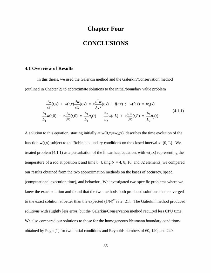
4.1 Overview of Results

In this thesis, we used the Galerkin method and the Galerkin/Conservation method

(outlined in Chapter 2) to approximate solutions to the initial/boundary value problem

A solution to this equation, starting initially at w(0,x)=w (x), describes the time evolution of the0

function w(t,x) subject to the Robin’s boundary conditions on the closed interval x0[0, L]. We

treated problem (4.1.1) as a perturbation of the linear heat equation, with w(t,x) representing the

temperature of a rod at position x and time t. Using N = 4, 8, 16, and 32 elements, we compared

our results obtained from the two approximation methods on the bases of accuracy, speed

(computational execution time), and behavior. We investigated two specific problems where we

knew the exact solution and found that the two methods both produced solutions that converged

to the exact solution at better than the expected (1/N) rate [21]. The Galerkin method produced½

solutions with slightly less error, but the Galerkin/Conservation method required less CPU time.

We also compared our solutions to those for the homogeneous Neumann boundary conditions

obtained by Pugh [1] for two initial conditions and Reynolds numbers of 60, 120, and 240.

86

Again, both methods produced virtually identical results except for one case where the Galerkin

solution grew exponentially in time despite the convergent behavior of the Galerkin/Conservation

solution. These reults are similar to what was obtained by Pugh [1]. Since the

Galerkin/Conservation method is also generally faster with respect to computation time, we

conclude that it is “better” in the sense that it is computationally more efficient.

We also investigated the cases when the Robin’s boundary conditions were allowed to

approach both the Dirichlet and the Neumann boundary conditions. We looked at two examples

for each case. For the Dirichlet case, we let L =L approach zero (or 6 =6 64), representing a1 2 1 2

very thin film (or a very good conductor) on each end of the rod. In both examples, the solutions

seemed to uniformly approach a limiting solution as L =L approached zero. For the Neumann1 2

case, we let L =L approach infinity (or 6 =6 60), representing a very thick film (or a very good1 2 1 2

insulator) on each end of the rod. These thick films act as insulators, allowing us to approach the

Neumann case, which corresponds to films composed of perfect insulators. We produced the

Neumann solution by setting 6 =6 =0, for comparison. In both examples, our solution seemed to1 2

uniformly approach the Neumann solution as L =L approached infinity. However, the solutions1 2

using the Robin’s appeared to reach zero at some large time, where the Neumann solution

seemed to have reached a nonconstant steady state.

4.2 Conclusions

The numerical results contained in this paper are consistent with Burns et.al. [2]. We

seemed to obtain nonconstant steady state solutions for certain initial conditions and Reynolds

numbers using “exact” Neumann boundary conditions. However, when the more realistic Robin’s

87

boundary conditions are employed, our results seem to show that the solutions will reach zero in

the steady state. However, if L =L are large enough, we would expect to see nonconstant steady1 2

state solutions due to computational errors, as described in [2].

Our numerical results suggest that when the Robin’s boundary conditions are allowed to

approach the Dirichlet and the Neumann boundary conditions, the solutions obtained approach

the solutions corresponding to the Dirichlet and Neumann problems respectively. This could be

very useful in cases where the solutions for the “exact” Dirichlet and Neumann problems are not

easily obtainable by direct computation.

4.3 Open Problems

Our numerical results give rise to several interesting questions. It is our hope that we

have provided motivation for research into the following areas:

< Can one prove that the solutions for the Robin’s boundary conditions approach the

Dirichlet and Neumann solutions as the Robin’s boundary conditions are allowed

to approach the Dirichlet and Neumann boundary condition, respectively?

< Can the methods of this paper be successfully applied to other areas of research on

Burgers’ equation, e.g. control theory? This question is being investigated in part

by Massa [20].

< Can one prove that non-constant steady state solutions exist for the Burgers’

equation with Robin’s boundary conditions?

88

Appendix A

MATLAB CODE

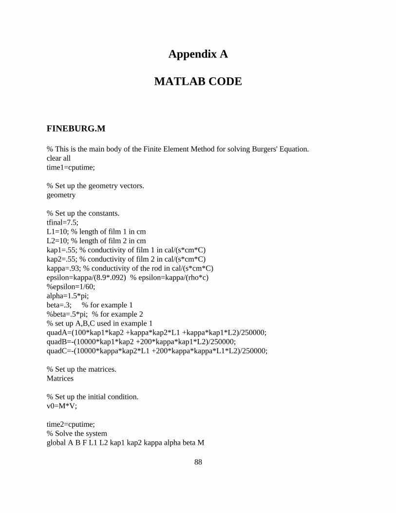
FINEBURG.M

% This is the main body of the Finite Element Method for solving Burgers' Equation. clear alltime1=cputime;

% Set up the geometry vectors.geometry

% Set up the constants.tfinal=7.5;L1=10; % length of film 1 in cmL2=10; % length of film 2 in cmkap1=.55; % conductivity of film 1 in cal/(s*cm*C)kap2=.55; % conductivity of film 2 in cal/(s*cm*C)kappa=.93; % conductivity of the rod in cal/(s*cm*C)epsilon=kappa/(8.9*.092) % epsilon=kappa/(rho*c)%epsilon=1/60;alpha=1.5*pi;beta=.3; % for example 1%beta=.5*pi; % for example 2% set up A,B,C used in example 1quadA=(100*kap1*kap2 +kappa*kap2*L1 +kappa*kap1*L2)/250000;quadB=-(10000*kap1*kap2 +200*kappa*kap1*L2)/250000;quadC=-(10000*kappa*kap2*L1 +200*kappa*kappa*L1*L2)/250000;

% Set up the matrices. Matrices

% Set up the initial condition.v0=M*V;

time2=cputime;% Solve the systemglobal A B F L1 L2 kap1 kap2 kappa alpha beta M

89

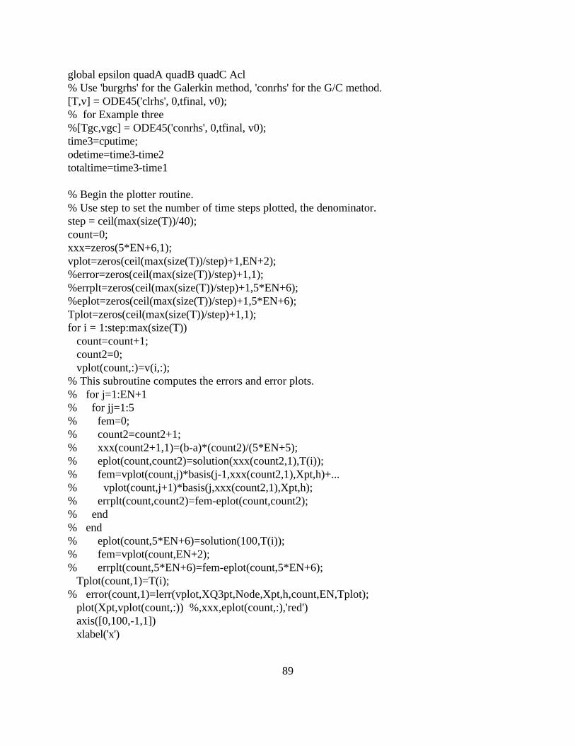
global epsilon quadA quadB quadC Acl% Use 'burgrhs' for the Galerkin method, 'conrhs' for the G/C method.[T,v] = ODE45('clrhs', 0,tfinal, v0);% for Example three%[Tgc,vgc] = ODE45('conrhs', 0,tfinal, v0);time3=cputime;odetime=time3-time2totaltime=time3-time1

% Begin the plotter routine.% Use step to set the number of time steps plotted, the denominator.step = ceil(max(size(T))/40);count=0;xxx=zeros(5*EN+6,1);vplot=zeros(ceil(max(size(T))/step)+1,EN+2);%error=zeros(ceil(max(size(T))/step)+1,1);%errplt=zeros(ceil(max(size(T))/step)+1,5*EN+6);%eplot=zeros(ceil(max(size(T))/step)+1,5*EN+6);Tplot=zeros(ceil(max(size(T))/step)+1,1);for i = 1:step:max(size(T)) count=count+1; count2=0; vplot(count,:)=v(i,:);% This subroutine computes the errors and error plots.% for j=1:EN+1% for jj=1:5% fem=0;% count2=count2+1;% xxx(count2+1,1)=(b-a)*(count2)/(5*EN+5);% eplot(count,count2)=solution(xxx(count2,1),T(i));% fem=vplot(count,j)*basis(j-1,xxx(count2,1),Xpt,h)+...% vplot(count,j+1)*basis(j,xxx(count2,1),Xpt,h);% errplt(count,count2)=fem-eplot(count,count2);% end% end% eplot(count,5*EN+6)=solution(100,T(i));% fem=vplot(count,EN+2);% errplt(count,5*EN+6)=fem-eplot(count,5*EN+6); Tplot(count,1)=T(i);% error(count,1)=lerr(vplot,XQ3pt,Node,Xpt,h,count,EN,Tplot); plot(Xpt,vplot(count,:)) %,xxx,eplot(count,:),'red') axis([0,100,-1,1]) xlabel('x')

90

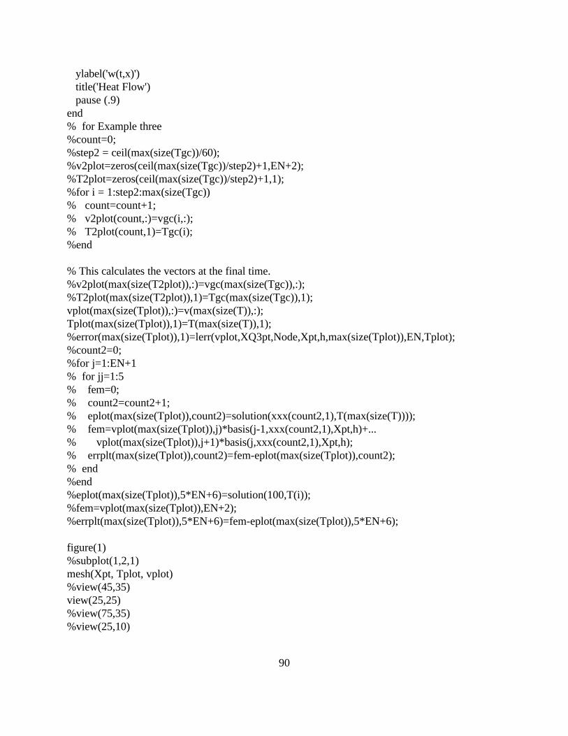
ylabel('w(t,x)') title('Heat Flow') pause (.9)end% for Example three%count=0;%step2 = ceil(max(size(Tgc))/60);%v2plot=zeros(ceil(max(size(Tgc))/step2)+1,EN+2);%T2plot=zeros(ceil(max(size(Tgc))/step2)+1,1);%for i = 1:step2:max(size(Tgc))% count=count+1;% v2plot(count,:)=vgc(i,:);% T2plot(count,1)=Tgc(i);%end

% This calculates the vectors at the final time.%v2plot(max(size(T2plot)),:)=vgc(max(size(Tgc)),:);%T2plot(max(size(T2plot)),1)=Tgc(max(size(Tgc)),1);vplot(max(size(Tplot)),:)=v(max(size(T)),:);Tplot(max(size(Tplot)),1)=T(max(size(T)),1);%error(max(size(Tplot)),1)=lerr(vplot,XQ3pt,Node,Xpt,h,max(size(Tplot)),EN,Tplot);%count2=0;%for j=1:EN+1% for jj=1:5% fem=0;% count2=count2+1;% eplot(max(size(Tplot)),count2)=solution(xxx(count2,1),T(max(size(T))));% fem=vplot(max(size(Tplot)),j)*basis(j-1,xxx(count2,1),Xpt,h)+...% vplot(max(size(Tplot)),j+1)*basis(j,xxx(count2,1),Xpt,h);% errplt(max(size(Tplot)),count2)=fem-eplot(max(size(Tplot)),count2);% end%end%eplot(max(size(Tplot)),5*EN+6)=solution(100,T(i));%fem=vplot(max(size(Tplot)),EN+2);%errplt(max(size(Tplot)),5*EN+6)=fem-eplot(max(size(Tplot)),5*EN+6);

figure(1)%subplot(1,2,1)mesh(Xpt, Tplot, vplot)%view(45,35)view(25,25)%view(75,35) %view(25,10)

91

%COLORMAP([1 1 1])% Example one and six%axis([0,100,0,tfinal,-.4,.4])% Example two and sevenaxis([0,100,0,tfinal,-1,1])% Example three%axis([0,1,0,10,-1.5,1.5])% Example four%axis([0,100,0,tfinal,-.5,.5])% Example five%axis([0,100,0,tfinal,0,.4])grid xlabel('x') ylabel('t') zlabel('w(t,x)') title('Numerical Solution')%figure(2)%subplot(1,2,2)%mesh(Xpt, T2plot, v2plot)%view(75,35)%view(25,10)%COLORMAP([1 1 1])%axis([0,100,0,tfinal,-.4,.4])%grid% xlabel('x')% ylabel('t')% zlabel('w(t,x)')% title('Numerical Solution')% Plot the exact solution.%figure(3)%mesh(xxx, Tplot, eplot)%view(75,35)%grid%COLORMAP([1 1 1])%axis([0,100,0,tfinal,-1,1])% xlabel('x')% ylabel('t')% zlabel('w(t,x)')% title('Exact Solution')% Plot the error.%figure (3)%mesh(xxx, Tplot, errplt)%view(75,35)

92

%grid% Example one%axis([0,100,0,tfinal,-.1,.1])% Example two%axis([0,100,0,tfinal,-.02,.02])% xlabel('x')% ylabel('t')% zlabel('wN(t,x) - w(t,x)')% title('Error')

GEOMETRY.M

%This script sets up the necessary arrays that allow the main program%to compute results for a specific problem. Contained herein is the %correspondence between the actual layout of the problem and the %layout of the functions used in the main program.%===================================================================

% a, b are the endpoints. EN the number of internal nodes.a=0;b=100;EN=16;

% step-size if uniform.unifh=(1/(EN+1))*(b-a)numint=(b-a)/unifh;h=0;for i=1:numint, h(i)=unifh;, end% step-size if not uniform.%h=[.1 .2 .3 .4];

% Total number of nodes.numnode=max(size(h))+1;

% Set up the x-coordinate of each node.Xpt=zeros(numnode,1);Xpt(1) = a;for i=2:numnode, Xpt(i)=Xpt(i-1)+h(i-1);, end

% Set up Index, which describes the number of unknowns at each global unknown.Index=zeros(numnode,1);for i=1:numnode

93

Index(i)=i;end

% Set up the 1-pt. quadrature points in each element.XQpt=0;for i=1:max(size(h)), XQpt(i,1)=Xpt(i)+h(i)/2;, end%nquad=1;

% Set up the 2-pt. quadrature points.XQSpt=0;for i=1:max(size(XQpt)), XQSpt(i,1)=XQpt(i) - .5773502692*h(i)/2; XQSpt(i,2)=XQpt(i) + .5773502692*h(i)/2;end

% Set up the 3-pt. quadrature points.XQ3pt=0;for i=1:max(size(XQpt)), XQ3pt(i,1)=XQpt(i) - .7745966692*h(i)/2; XQ3pt(i,2)=XQpt(i); XQ3pt(i,3)=XQpt(i) + .7745966692*h(i)/2;end

% Set up the relation between the local node for the basis %functions and the global nodes.Node=zeros(max(size(h)),2);for i=1:max(size(h)), Node(i,1)=i;,endfor i=1:max(size(h)), Node(i,2)=i+1;, endnlocal=2;

BASIS.M

function y = basis(z,x,Xpt,h)

% This function gives the value of the basis function at a given node.%z is which basis function it is and x is the value at which to evaluate.

temp1=0;%---------Fix it for z=0-----------if z==0 if temp1==0

if x<Xpt(2)

94

y=(Xpt(2)-x)/(h(1));temp1 =1;end

end if temp1==0

y=0;temp1=1;

endend%---------Fix it for z=max(size(Xpt))--------if z==max(size(Xpt))-1 if temp1==0

if x<Xpt(z)y=0;temp1=1;end

end if temp1==0

y=(x-Xpt(z))/h(z);temp1 =1;

endend%----------------------------------if temp1==0

if x<Xpt(z)y=0;temp1 =1;end

endif temp1==0

if x<Xpt(z+1)y=(x-Xpt(z))/h(z);temp1 =1;end

endif temp1==0

if x<Xpt(z+2)y=(Xpt(z+2)-x)/(h(z+1));temp1 =1;end

endif temp1==0

if x<=1

95

y=0;temp1 =1;end

end

BASISD.M

function y = basisd(z,x,Xpt,h)

% This function gives the value of the derivative of the basis function at a given node.%z is which basis function it is and x is the value at which to evaluate.

temp1=0;%---------Fix it for z=0-----------if z==0 if temp1==0

if x<Xpt(2)y=-1/(h(1));temp1 =1;end

end if temp1==0

y=0;temp1=1;

endend%---------Fix it for z=max(size(Xpt))--------if z==max(size(Xpt))-1 if temp1==0

if x<Xpt(z)y=0;temp1=1;end

end if temp1==0

y=1/h(z);temp1 =1;

endend%----------------------------------if temp1==0

if x<Xpt(z)

96

y=0;temp1 =1;end

endif temp1==0

if x<Xpt(z+1)y=1/h(z);temp1 =1;end

endif temp1==0

if x<Xpt(z+2)y=-1/(h(z+1));temp1 =1;end

endif temp1==0

if x<=1y=0;temp1 =1;end

end

MATRICES.M

% This is the subroutine where the mass(MM) and stiffness(KK) matrices are assembled. % Build F(v), the inhomogeneous term matrix.

numunk=0;for i=1:max(size(Index))

if Index(i)>0,numunk=numunk+1;,endendMM=zeros(numunk,numunk);KK=zeros(numunk,numunk);FF=zeros(numunk,2);%FF=zeros(numunk,6); % for Example 2V=zeros(numunk,1);for nel=1:max(size(h)) for quad=1:2% quad=1; for j=1:nlocal if Index(Node(nel,j))>0

97

%integrate basis functions x=XQSpt(nel,quad); nnn=Index(Node(nel,j)); KK(nnn,nnn)=KK(nnn,nnn)-(basisd(nnn-1,x,Xpt,h)^2)*h(nel)/2; MM(nnn,nnn)=MM(nnn,nnn)+(basis(nnn-1,x,Xpt,h)^2)*h(nel)/2; if nnn<max(size(MM)) KK(nnn,nnn+1)=KK(nnn,nnn+1)-basisd(nnn-1,x,Xpt,h)*basisd(nnn,x,Xpt,h)*h(nel)/2; KK(nnn+1,nnn)=KK(nnn,nnn+1); MM(nnn,nnn+1)=MM(nnn,nnn+1)+basis(nnn-1,x,Xpt,h)*basis(nnn,x,Xpt,h)*h(nel)/2; MM(nnn+1,nnn)=MM(nnn,nnn+1); end %integrate basis functions against f(x)% Example one% FF(nnn,1)=FF(nnn,1)-(beta*(quadA*x*x+quadB*x+quadC+(sin(.01*pi*x))^2)+ ...% epsilon*(2*quadA+.0002*pi*pi*((cos(.01*pi*x))^2 - ...% (sin(.01*pi*x))^2)))*basis(nnn-1,x,Xpt,h)*h(nel)/2;% FF(nnn,2)=FF(nnn,2)+(quadA*x*x+quadB*x+quadC+(sin(.01*pi*x))^2)* ...% (2*quadA*x+quadB+.02*pi*sin(.01*pi*x)*cos(.01*pi*x))* ...% basis(nnn-1,x,Xpt,h)*h(nel)/2;% Example two% FF(nnn,1)=FF(nnn,1)+.0001*alpha*((100-x)^2)*basis(nnn-1,x,Xpt,h)*h(nel)/2;% FF(nnn,2)=FF(nnn,2)-.0001*beta*(x^2)*basis(nnn-1,x,Xpt,h)*h(nel)/2;% FF(nnn,3)=FF(nnn,3)-(2/(10^8))*((100-x)^3)*basis(nnn-1,x,Xpt,h)*h(nel)/2;% FF(nnn,4)=FF(nnn,4)+(2/(10^8))*(x^3)*basis(nnn-1,x,Xpt,h)*h(nel)/2;% FF(nnn,5)=FF(nnn,5)+(4/(10^8))*(x^3-150*x*x+5000*x)*basis(nnn-1,x,Xpt,h)*h(nel)/2;% FF(nnn,6)=FF(nnn,6)-.0002*epsilon*basis(nnn-1,x,Xpt,h)*h(nel)/2;

%integrate basis functions against the initial function% Example one% V(nnn,1)=V(nnn,1)+(quadA*x*x+quadB*x+quadC+(sin(.01*pi*x))^2)* ...% basis(nnn-1,x,Xpt,h)*h(nel)/2;% Example two% V(nnn,1)=V(nnn,1)+.0001*(x^2)*basis(nnn-1,x,Xpt,h)*h(nel)/2;% Example three% V(nnn,1)=V(nnn,1)+.5cos(pi*x)*basis(nnn-1,x,Xpt,h)*h(nel)/2;% Example four% V(nnn,1)=V(nnn,1)+.5*cos(.01*pi*x)*basis(nnn-1,x,Xpt,h)*h(nel)/2;% Example five, six, seven V(nnn,1)=V(nnn,1)+cos(.01*pi*x)*basis(nnn-1,x,Xpt,h)*h(nel)/2; end end endend

98

% Adjust for the Robin's BCs.KK(1,1)=-1/h(1) - kap1/(kappa*L1);KK(numunk,numunk)=-1/h(numunk-1) - kap2/(kappa*L2);G=zeros(numunk,2);G(1,1)=kap1/(kappa*L1);G(numunk,2)=kap2/(kappa*L2);

M=inv(MM);A=M*KK;B=M*G;F=M*FF;

BURGRHS.M

function vdot = burgrhs(t,y)

% This function gives the right hand side for the Galerkin method.global A B F L1 L2 kap1 kap2 kappa alpha beta M global epsilon quadA quadB quadC

u=zeros(2,1);% Example two%u(1,1)=(1+.02*kappa*L1/kap1)*sin(alpha*t);%u(2,1)=(1+.02*kappa*L2/kap2)*cos(beta*t);

%H=zeros(2,1);% Example one%H(1,1)=exp(-beta*t);%H(2,1)=exp(-2*beta*t);

% Example two%H=zeros(6,1);%H(1,1)=cos(alpha*t);%H(2,1)=sin(beta*t);%H(3,1)=(sin(alpha*t))^2;%H(4,1)=(cos(beta*t))^2;%H(5,1)=sin(alpha*t)*cos(beta*t);%H(6,1)=sin(alpha*t) + cos(beta*t);

ll=max(size(y));J=zeros(ll,1);J(1,1)=-2*y(1)^2 +y(1)*y(2) + y(2)^2;

99

for i=2:ll-1 J(i,1)=-y(i-1)^2 -y(i-1)*y(i) + y(i)*y(i+1) + y(i+1)^2;endJ(ll,1)=-y(ll-1)^2 -y(ll-1)*y(ll)+2*y(ll)^2;J=(1/6)*J;

vdot = epsilon*(A*y +B*u) -M*J ; %+F*H;

CONRHS.M

function vdot = conrhs(t,y)

% This function gives the right hand side for the G/C method.global A B F L1 L2 kap1 kap2 kappa alpha beta M global epsilon quadA quadB quadC

u=zeros(2,1);% Example two%u(1,1)=(1+.02*kappa*L1/kap1)*sin(alpha*t);%u(2,1)=(1+.02*kappa*L2/kap2)*cos(beta*t);

%H=zeros(2,1);% Example one%H(1,1)=exp(-beta*t);%H(2,1)=exp(-2*beta*t);

% Example two%H=zeros(6,1);%H(1,1)=cos(alpha*t);%H(2,1)=sin(beta*t);%H(3,1)=(sin(alpha*t))^2;%H(4,1)=(cos(beta*t))^2;%H(5,1)=sin(alpha*t)*cos(beta*t);%H(6,1)=sin(alpha*t) + cos(beta*t);

ll=max(size(y));J=zeros(ll,1);J(1,1)=.25*(y(2)^2 - y(1)^2);for i=2:ll-1 J(i,1)=.25*(y(i+1)^2 - y(i-1)^2);endJ(ll,1)=.25*(y(ll)^2 - y(ll-1)^2);

100

vdot = epsilon*(A*y + B*u) -M*J; % +F*H;

SOLUTION.M

function y = solution(x,t)

% Set up the exact solution function.

global epsilon alpha beta quadA quadB quadC

% Example oney = exp(-beta*t)*(quadA*x*x + quadB*x + quadC + (sin(.01*pi*x))^2);

% Example two%y= .0001*((100-x)^2)*sin(alpha*t) + .0001*(x^2)*cos(beta*t);

%y = .25*cos(t)*cos(pi*x);

%y = .25*exp(-epsilon*t)*cos(pi*x);

%y = .25*exp(-epsilon*t)*(x*x+x-1);

%y = exp(-epsilon*t)*(quadA*x*x + quadB*x + quadC);

LERR.M

function y = lerr(vplot,XQ3pt,Node,Xpt,h,count,EN,Tplot)

% This function computes the L2 error in our finite element approximation.

err=0;for nel=1:EN+1 sol=zeros(3,1); fem=zeros(3,1); for quad=1:3 x=XQ3pt(nel,quad); for j=1:2 %nlocal %integrate the difference w-wh nnn=Node(nel,j); fem(quad,1)=fem(quad,1)+vplot(count,nnn)*basis(nnn-1,x,Xpt,h); end

101

sol(quad,1)=solution(x,Tplot(count)); end err=err+.55555556*((sol(3,1)-fem(3,1))^2+(sol(1,1)-fem(1,1))^2)*h(nel)/2 ... + .88888889*((sol(2,1)-fem(2,1))^2)*h(nel)/2;endy=(err)^.5;

102

1. Pugh, S.M., “Finite Element Approximations of Burgers’ Equation”, Virginia PolytechnicInstitute and State University, (1995).

2. Burns, J.A., Balogh, A., Gilliam, D.S., and Shubov, V.I., “Numerical Stationary Solutions fora Viscous Burgers’ Equation”, Journal of Mathematical Systems, Estimation, and Control, toappear.

3. Fourier, J. Théorie Analytique de la Chaleur. Paris, Didot, 1822.

4. Berg, P.W., and McGregor, J.L., Elementary Partial Differential Equations, Holden-Day,Oakland, California, (1966).

5. Sears, F.W., Zemansky, M.W., and Young, H.D., University Physics, Addison-Wesley,Reading, Massachusetts, (1988).

6. Schenck, Hilbert, Jr., Heat Transfer Engineering, Prentice-Hall, Englewood Cliffs, NJ,(1959).

7. Kern, D.Q., Process Heat Transfer, McGraw-Hill, New York, NY, (1950).

8. Incropera, F.P., and DeWitt, D.P., Fundamentals of Heat Transfer, John Wiley & Sons, NewYork, New York, (1981).

9. Widder, D.V., The Heat Equation, Academic Press, New York, New York, (1975).

10. Bateman, H., “Some Recent researches on the motion of fluids,” Mon. Weather Rev., 43,(1915).

11. Burgers, J.M., “Mathematical Examples Illustrating Relations Occurring in the Theory ofTurbulent Fluid Motion,” Trans. Roy. Neth. Acad. Sci., Amsterdam, 17, (1939), 1-53.

12. Fletcher, C.A.J., “Burgers’ Equation: A Model for All Reasons”, Numerical Solutions ofPartial Differential Equations, J. Noye (Editor), North-Holland Pub. Co. (1982).

13. Hopf, E., “The Partial Differential Equation u + uu = µu .”, Comm. Pure & Applied Math,t x xx

3, (1950), 201-230.

14. Cole, J.D., “On a Quasi-linear Parabolic Equation Occurring in Aerodynamics,” Quart. Appl.Math., 9, (1951), 225-236.

15. Byrnes, C.L., Gilliam, D.S., and Shubov, V.I., “Boundary Control, Feedback Stabilization,and the Existence of Attractors for a Viscous Burgers’ Equation,” (1990).

BIBLIOGRAPHY

103

16. Burns, J.A., and Kang, S., A control problem for Burgers’ equation with boundedinput/output, Institute for Computer Applications for Science and Engineering, ICASE Report90-45, (1990), NASA Langley Research Center, Hampton, VA.

17. Burns, J.A., and Kang, S., A stabilization problem for Burgers’ equation with unboundedcontrol and observation, International Series of Numerical Mathematics, Vol. 100, BirkhauserVerlag Basel, (1991).

18. Burden, R.L., Faires, J.D., Numerical Analysis, PWS Pub. Co., Boston, Massachusetts,(1993).

19. Marrekchi, H., “Dynamic Compensators for A Nonlinear Conservation Law,” Virginia Tech,(1993).

20. Massa, K.L., “Computational Analysis and Control of Burgers’ Equation,” M.S. Thesis,Virginia Tech, (1997).

21. Fletcher, C.A.J., Computational Galerkin Methods, Springer-Verlag, New York, New York,(1984).

Documents

Finite Element Approximations of Burgers' Equation - Virginia Tech