Embed Size (px)
Citation preview
Finite Element Analysis
Prof. Dr.B.N.Rao
Department of Civil Engineering
Indian Institute of Technology, Madras
Lecture - 35
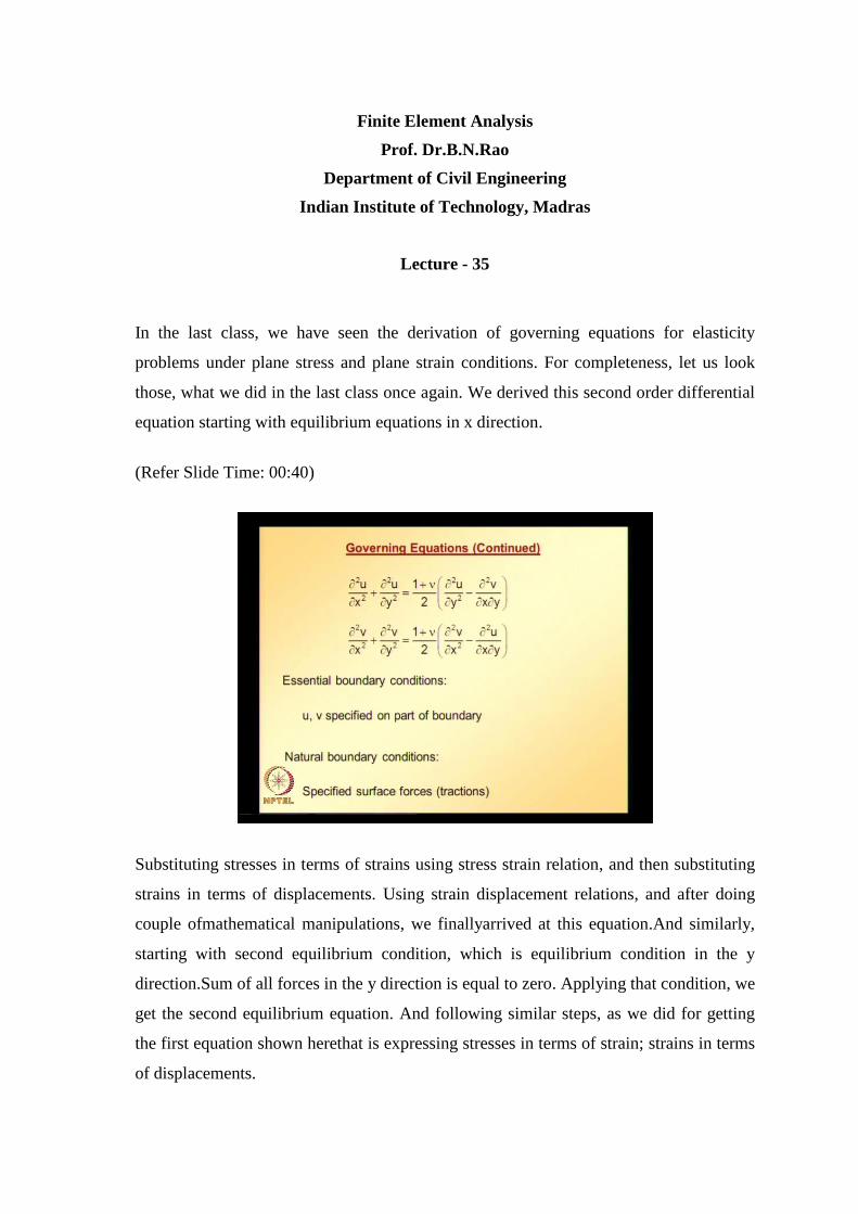
In the last class, we have seen the derivation of governing equations for elasticity
problems under plane stress and plane strain conditions. For completeness, let us look
those, what we did in the last class once again. We derived this second order differential
equation starting with equilibrium equations in x direction.
(Refer Slide Time: 00:40)
Substituting stresses in terms of strains using stress strain relation, and then substituting
strains in terms of displacements. Using strain displacement relations, and after doing
couple ofmathematical manipulations, we finallyarrived at this equation.And similarly,
starting with second equilibrium condition, which is equilibrium condition in the y
direction.Sum of all forces in the y direction is equal to zero. Applying that condition, we
get the second equilibrium equation. And following similar steps, as we did for getting
the first equation shown herethat is expressing stresses in terms of strain; strains in terms
of displacements.
And doing couple of mathematical manipulations finally, we arrive at the second
differential equation, which is also second order differential equations. And so, solution
for a three dimensional elasticity problemis basically solving these two coupled second
order differential equations subjected to boundary conditions.u and v specified on part of
boundary and you can notice here, these two are second order differential equations. So,
those boundary conditions of order 0 are essential boundary conditions and those
boundary conditions of order one are natural boundary conditions.
And natural boundary conditions are specified surface tractions and when I made this
statement that, the specified surface forces are first order equations. That is based on
similar to what we did in last class, that is expressed tractions in terms of stresses and
stresses in terms of displacements via stress strain and strain displacement relations.
Finally, we can see tractions are related to first derivative of displacements, which are
natural boundary conditions.
(Refer Slide Time: 03:23)
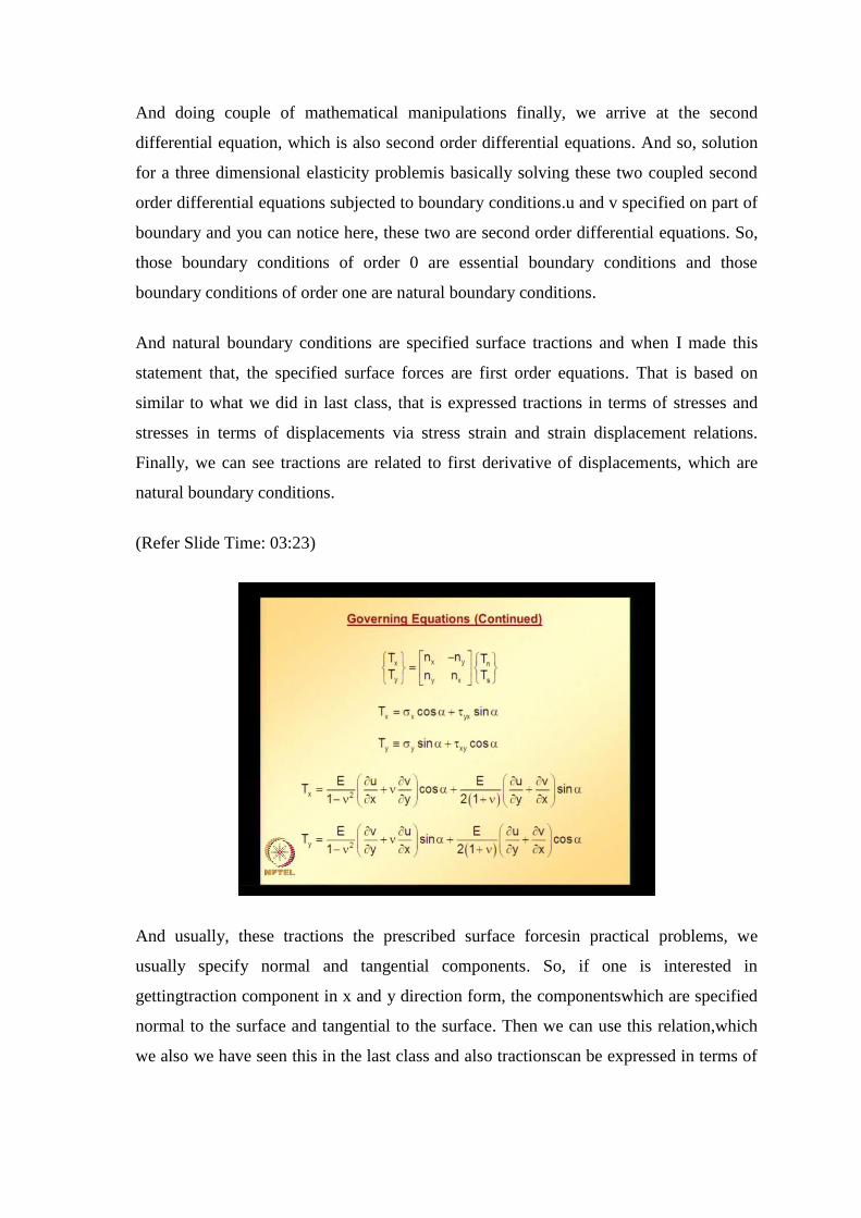
And usually, these tractions the prescribed surface forcesin practical problems, we
usually specify normal and tangential components. So, if one is interested in
gettingtraction component in x and y direction form, the componentswhich are specified
normal to the surface and tangential to the surface. Then we can use this relation,which
we also we have seen this in the last class and also tractionscan be expressed in terms of
internal stresses; writing equilibrium equation for a triangle showing the surface tractions
and internal stress components.In the last class, we have seen how to get this equation.
Similarly, tractions in the y directions can also be expressed in terms of stresses and now,
replacing stresses in terms of strains and strains in terms of displacements. We can see
that, traction in x direction is indeed related to derivative of displacements. Similarly,
traction in the y direction is related to derivative of displacements. So, natural boundary
conditions are indeed first order equations.So, solving an elasticity problem is basically
solving coupled differential second order differential equations that we have seen.In the
previous line subjected to the boundary conditions that u and v are specified on a part of
boundary ortractions are specified on a part of boundary.
(Refer Slide Time: 05:29)
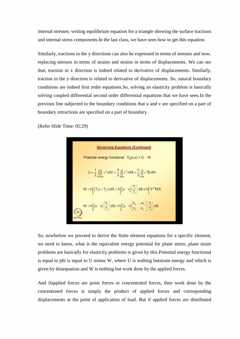
So, nowbefore we proceed to derive the finite element equations for a specific element,
we need to know, what is the equivalent energy potential for plane stress; plane strain
problems are basically for elasticity problems is given by this.Potential energy functional
is equal to phi is equal to U minus W, where U is nothing butstrain energy and which is
given by thisequation and W is nothing but work done by the applied forces.
And ifapplied forces are point forces or concentrated forces, then work done by the
concentrated forces is simply the product of applied forces and corresponding
displacements at the point of application of load. But if applied forces are distributed
forces then, work done due to applied forces can be calculated using this relation.In both
these relations U and W, h thickness is assumed to be constant.So, it is pulled out of the
integral and if it is not constant, then we need to take inside the integral and thendo the
integration.
And if these tractions T x T y basically, if they are given in terms of T n and T s that is
tangential and normal components,in that case work done by thedistributedforces can be
calculated using this relation.So, this is how, we can calculate U and W. Once we get U
and W, we can plug in into phi; phi is equal to U minus W.And apply the condition that
variation of phi is equal to 0 to get the finalelement equations. So, now let us start with
by taking a three node linear triangular element and derive the element equations for that
particular element.
(Refer Slide Time: 07:49)
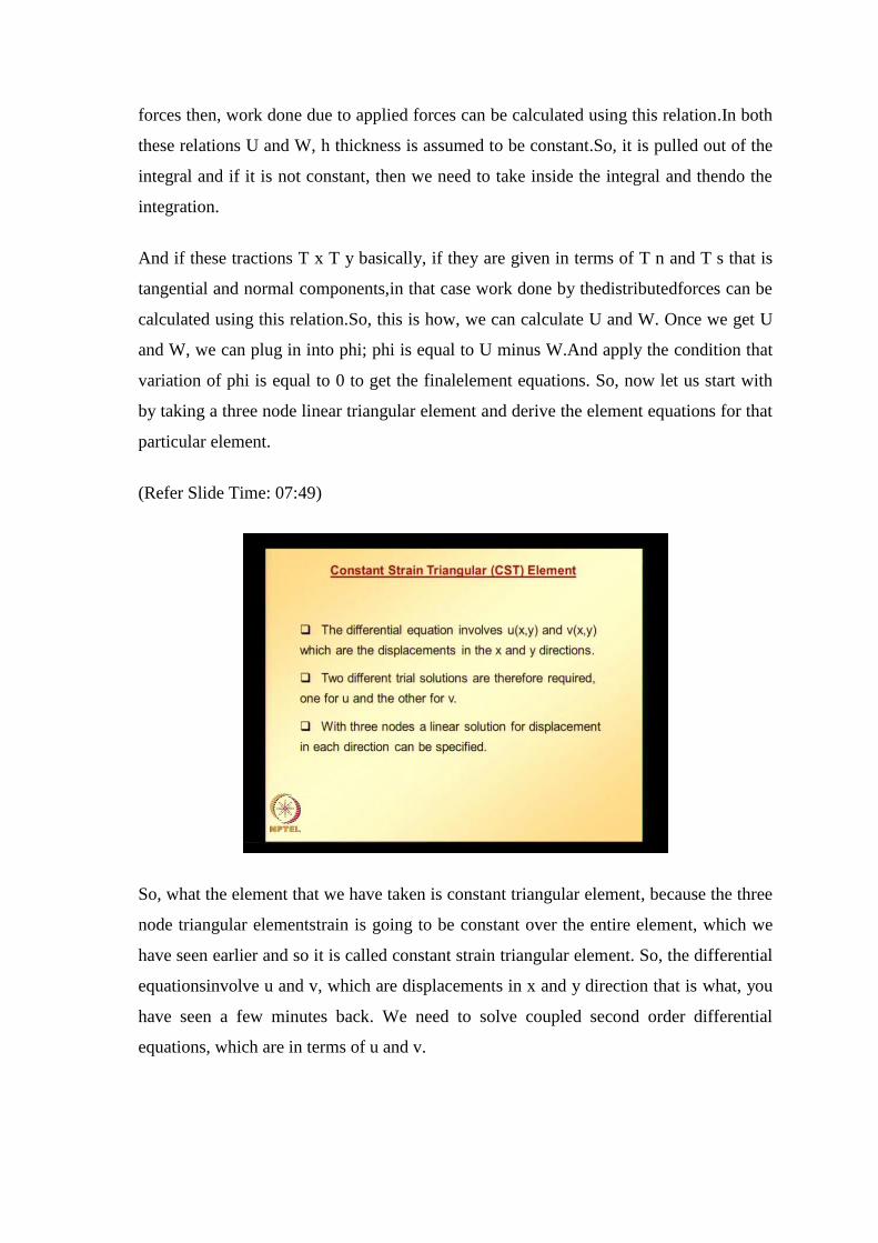
So, what the element that we have taken is constant triangular element, because the three
node triangular elementstrain is going to be constant over the entire element, which we
have seen earlier and so it is called constant strain triangular element. So, the differential
equationsinvolve u and v, which are displacements in x and y direction that is what, you
have seen a few minutes back. We need to solve coupled second order differential
equations, which are in terms of u and v.
u and v are nothing butdisplacements in the x and y directions, which are going to be
functions of x and y. So, we require two different trial solutions; one for displacement in
the x direction;the other for displacement in the y direction.With three nodes a linear
solution for displacements in each direction can be specified. So, now let us consider a
typical three node element and x try to express this displacement at any point in the
element in terms ofnodal values and shape functions.
(Refer Slide Time: 09:28)
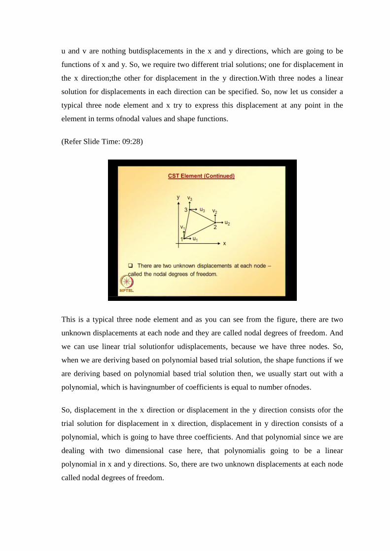
This is a typical three node element and as you can see from the figure, there are two
unknown displacements at each node and they are called nodal degrees of freedom. And
we can use linear trial solutionfor udisplacements, because we have three nodes. So,
when we are deriving based on polynomial based trial solution, the shape functions if we
are deriving based on polynomial based trial solution then, we usually start out with a
polynomial, which is havingnumber of coefficients is equal to number ofnodes.
So, displacement in the x direction or displacement in the y direction consists ofor the
trial solution for displacement in x direction, displacement in y direction consists of a
polynomial, which is going to have three coefficients. And that polynomial since we are
dealing with two dimensional case here, that polynomialis going to be a linear
polynomial in x and y directions. So, there are two unknown displacements at each node
called nodal degrees of freedom.
(Refer Slide Time: 11:06)
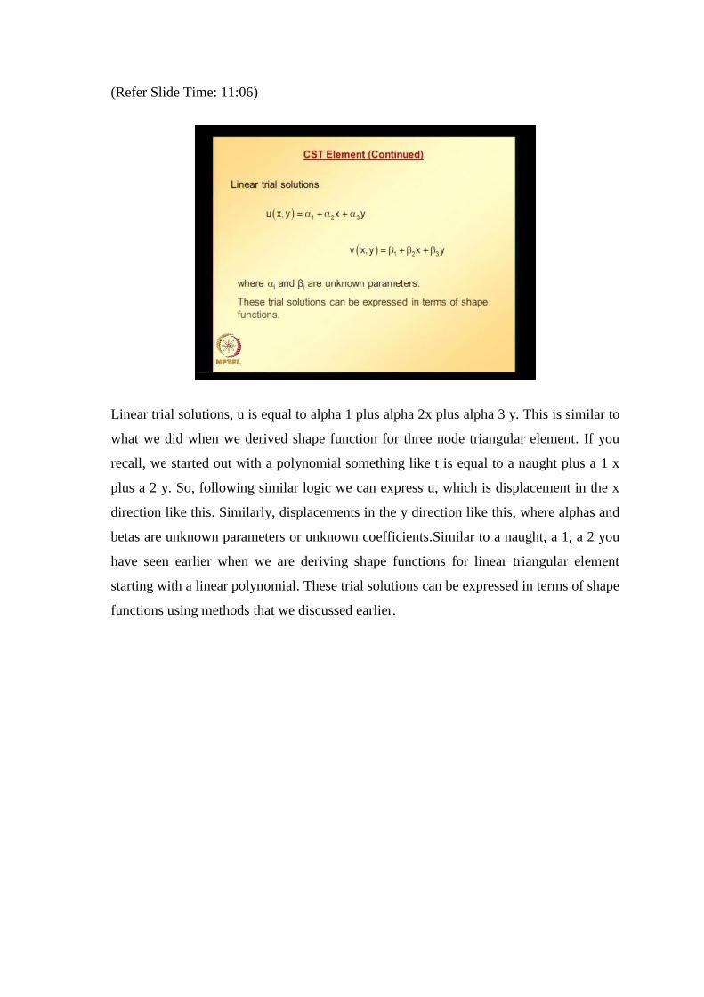
Linear trial solutions, u is equal to alpha 1 plus alpha 2x plus alpha 3 y. This is similar to
what we did when we derived shape function for three node triangular element. If you
recall, we started out with a polynomial something like t is equal to a naught plus a 1 x
plus a 2 y. So, following similar logic we can express u, which is displacement in the x
direction like this. Similarly, displacements in the y direction like this, where alphas and
betas are unknown parameters or unknown coefficients.Similar to a naught, a 1, a 2 you
have seen earlier when we are deriving shape functions for linear triangular element
starting with a linear polynomial. These trial solutions can be expressed in terms of shape
functions using methods that we discussed earlier.
(Refer Slide Time: 12:36)
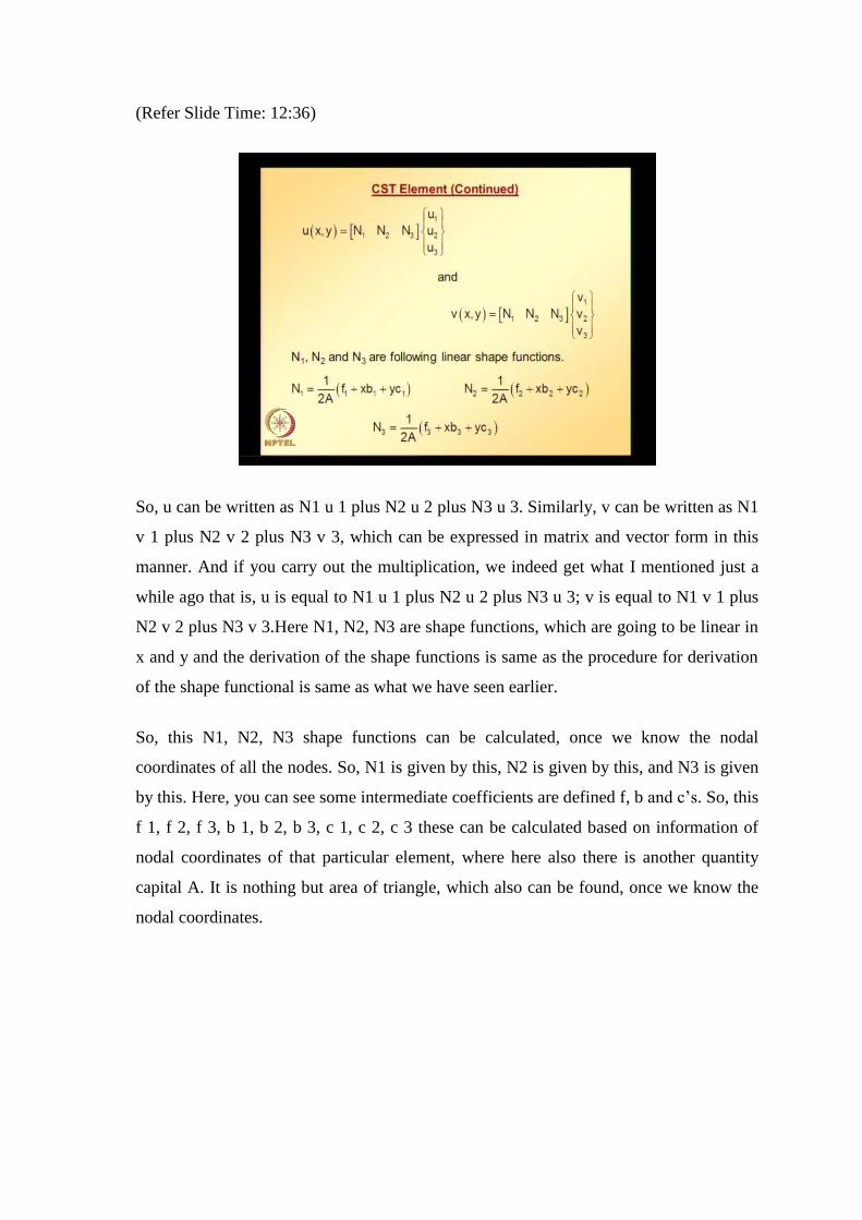
So, u can be written as N1 u 1 plus N2 u 2 plus N3 u 3. Similarly, v can be written as N1
v 1 plus N2 v 2 plus N3 v 3, which can be expressed in matrix and vector form in this
manner. And if you carry out the multiplication, we indeed get what I mentioned just a
while ago that is, u is equal to N1 u 1 plus N2 u 2 plus N3 u 3; v is equal to N1 v 1 plus
N2 v 2 plus N3 v 3.Here N1, N2, N3 are shape functions, which are going to be linear in
x and y and the derivation of the shape functions is same as the procedure for derivation
of the shape functional is same as what we have seen earlier.
So, this N1, N2, N3 shape functions can be calculated, once we know the nodal
coordinates of all the nodes. So, N1 is given by this, N2 is given by this, and N3 is given
by this. Here, you can see some intermediate coefficients are defined f, b and c’s. So, this
f 1, f 2, f 3, b 1, b 2, b 3, c 1, c 2, c 3 these can be calculated based on information of
nodal coordinates of that particular element, where here also there is another quantity
capital A. It is nothing but area of triangle, which also can be found, once we know the
nodal coordinates.
(Refer Slide Time: 14:17)
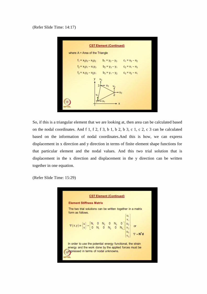
So, if this is a triangular element that we are looking at, then area can be calculated based
on the nodal coordinates. And f 1, f 2, f 3, b 1, b 2, b 3, c 1, c 2, c 3 can be calculated
based on the information of nodal coordinates.And this is how, we can express
displacement in x direction and y direction in terms of finite element shape functions for
that particular element and the nodal values. And this two trial solution that is
displacement in the x direction and displacement in the y direction can be written
together in one equation.
(Refer Slide Time: 15:29)
So, we will be looking at how to derive element stiffness matrix, because we haveseen
how to express displacement in x direction y direction in terms of finite element shape
functions and nodal values. Now, we are ready to derive element stiffness matrix. As I
just mentioned, the trial solution x and y direction can be written together in a matrix
form. Or compactly, it can be written as psi is equal to N transpose d, where n comprises
of all or N is the vector or matrix consisting of all the shape function expressions.
And d is nothing but,vector of nodal parameters or nodal unknowns and here, this is
how, displacement in x direction and y direction can be interpolated using finite element
shape functions and nodal values.Butif you go back and see, the strain energy equation u;
it consists of strains. So, in order to use potential energy functional, the strain energy and
work done by the applied forces must be expressed in terms of displacements or in terms
of nodal unknowns.Strain energy in terms of nodal unknowns can be written as follows.
(Refer Slide Time: 16:54)
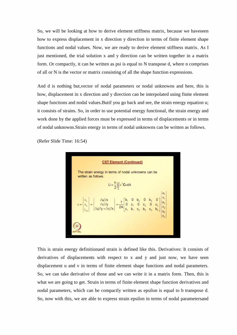
This is strain energy definitionand strain is defined like this. Derivatives: It consists of
derivatives of displacements with respect to x and y and just now, we have seen
displacement u and v in terms of finite element shape functions and nodal parameters.
So, we can take derivative of those and we can write it in a matrix form. Then, this is
what we are going to get. Strain in terms of finite element shape function derivatives and
nodal parameters, which can be compactly written as epsilon is equal to b transpose d.
So, now with this, we are able to express strain epsilon in terms of nodal parametersand
b matrix consists of derivatives of shape functions. So, substituting this epsilon into the
equation for u, we get this one.
(Refer Slide Time: 18:29)
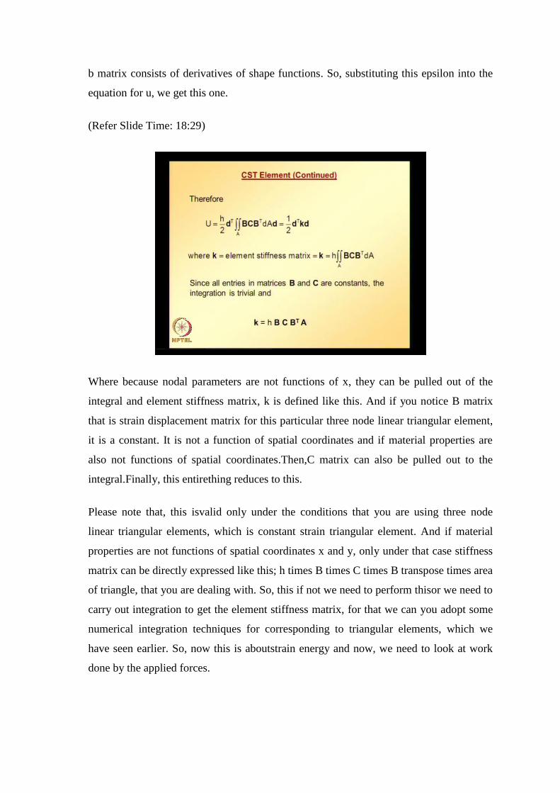
Where because nodal parameters are not functions of x, they can be pulled out of the
integral and element stiffness matrix, k is defined like this. And if you notice B matrix
that is strain displacement matrix for this particular three node linear triangular element,
it is a constant. It is not a function of spatial coordinates and if material properties are
also not functions of spatial coordinates.Then,C matrix can also be pulled out to the
integral.Finally, this entirething reduces to this.
Please note that, this isvalid only under the conditions that you are using three node
linear triangular elements, which is constant strain triangular element. And if material
properties are not functions of spatial coordinates x and y, only under that case stiffness
matrix can be directly expressed like this; h times B times C times B transpose times area
of triangle, that you are dealing with. So, this if not we need to perform thisor we need to
carry out integration to get the element stiffness matrix, for that we can you adopt some
numerical integration techniques for corresponding to triangular elements, which we
have seen earlier. So, now this is aboutstrain energy and now, we need to look at work
done by the applied forces.
(Refer Slide Time: 20:44)
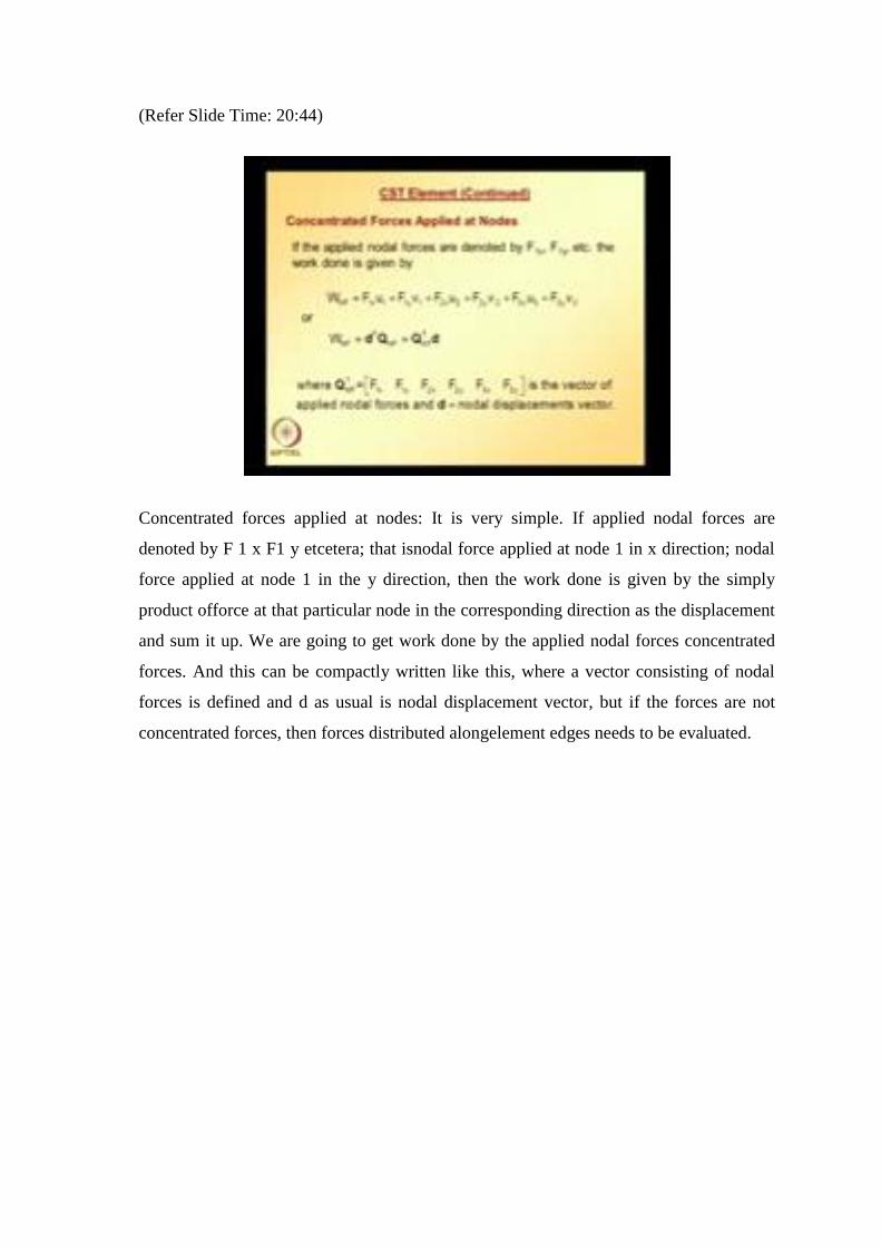
Concentrated forces applied at nodes: It is very simple. If applied nodal forces are
denoted by F 1 x F1 y etcetera; that isnodal force applied at node 1 in x direction; nodal
force applied at node 1 in the y direction, then the work done is given by the simply
product offorce at that particular node in the corresponding direction as the displacement
and sum it up. We are going to get work done by the applied nodal forces concentrated
forces. And this can be compactly written like this, where a vector consisting of nodal
forces is defined and d as usual is nodal displacement vector, but if the forces are not
concentrated forces, then forces distributed alongelement edges needs to be evaluated.
(Refer Slide Time: 21:55)
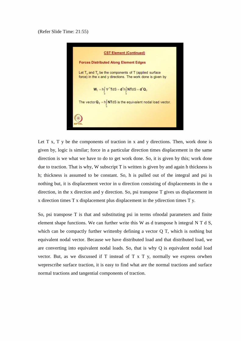
Let T x, T y be the components of traction in x and y directions. Then, work done is
given by, logic is similar; force in a particular direction times displacement in the same
direction is we what we have to do to get work done. So, it is given by this; work done
due to traction. That is why, W subscript T is written is given by and again h thickness is
h; thickness is assumed to be constant. So, h is pulled out of the integral and psi is
nothing but, it is displacement vector in u direction consisting of displacements in the u
direction, in the x direction and y direction. So, psi transpose T gives us displacement in
x direction times T x displacement plus displacement in the ydirection times T y.
So, psi transpose T is that and substituting psi in terms ofnodal parameters and finite
element shape functions. We can further write this W as d transpose h integral N T d S,
which can be compactly further writtenby defining a vector Q T, which is nothing but
equivalent nodal vector. Because we have distributed load and that distributed load, we
are converting into equivalent nodal loads. So, that is why Q is equivalent nodal load
vector. But, as we discussed if T instead of T x T y, normally we express orwhen
weprescribe surface traction, it is easy to find what are the normal tractions and surface
normal tractions and tangential components of traction.
(Refer Slide Time: 24:14)
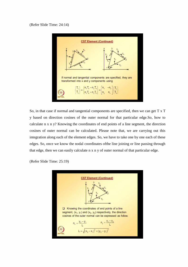
So, in that case if normal and tangential components are specified, then we can get T x T
y based on direction cosines of the outer normal for that particular edge.So, how to
calculate n x n y? Knowing the coordinates of end points of a line segment, the direction
cosines of outer normal can be calculated. Please note that, we are carrying out this
integration along each of the element edges. So, we have to take one by one each of these
edges. So, once we know the nodal coordinates ofthe line joining or line passing through
that edge, then we can easily calculate n x n y of outer normal of that particular edge.
(Refer Slide Time: 25:19)
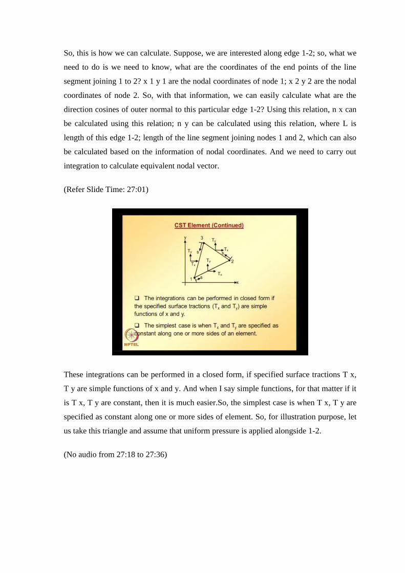
So, this is how we can calculate. Suppose, we are interested along edge 1-2; so, what we
need to do is we need to know, what are the coordinates of the end points of the line
segment joining 1 to 2? x 1 y 1 are the nodal coordinates of node 1; x 2 y 2 are the nodal
coordinates of node 2. So, with that information, we can easily calculate what are the
direction cosines of outer normal to this particular edge 1-2? Using this relation, n x can
be calculated using this relation; n y can be calculated using this relation, where L is
length of this edge 1-2; length of the line segment joining nodes 1 and 2, which can also
be calculated based on the information of nodal coordinates. And we need to carry out
integration to calculate equivalent nodal vector.
(Refer Slide Time: 27:01)
These integrations can be performed in a closed form, if specified surface tractions T x,
T y are simple functions of x and y. And when I say simple functions, for that matter if it
is T x, T y are constant, then it is much easier.So, the simplest case is when T x, T y are
specified as constant along one or more sides of element. So, for illustration purpose, let
us take this triangle and assume that uniform pressure is applied alongside 1-2.
(No audio from 27:18 to 27:36)
(Refer Slide Time: 27:32)
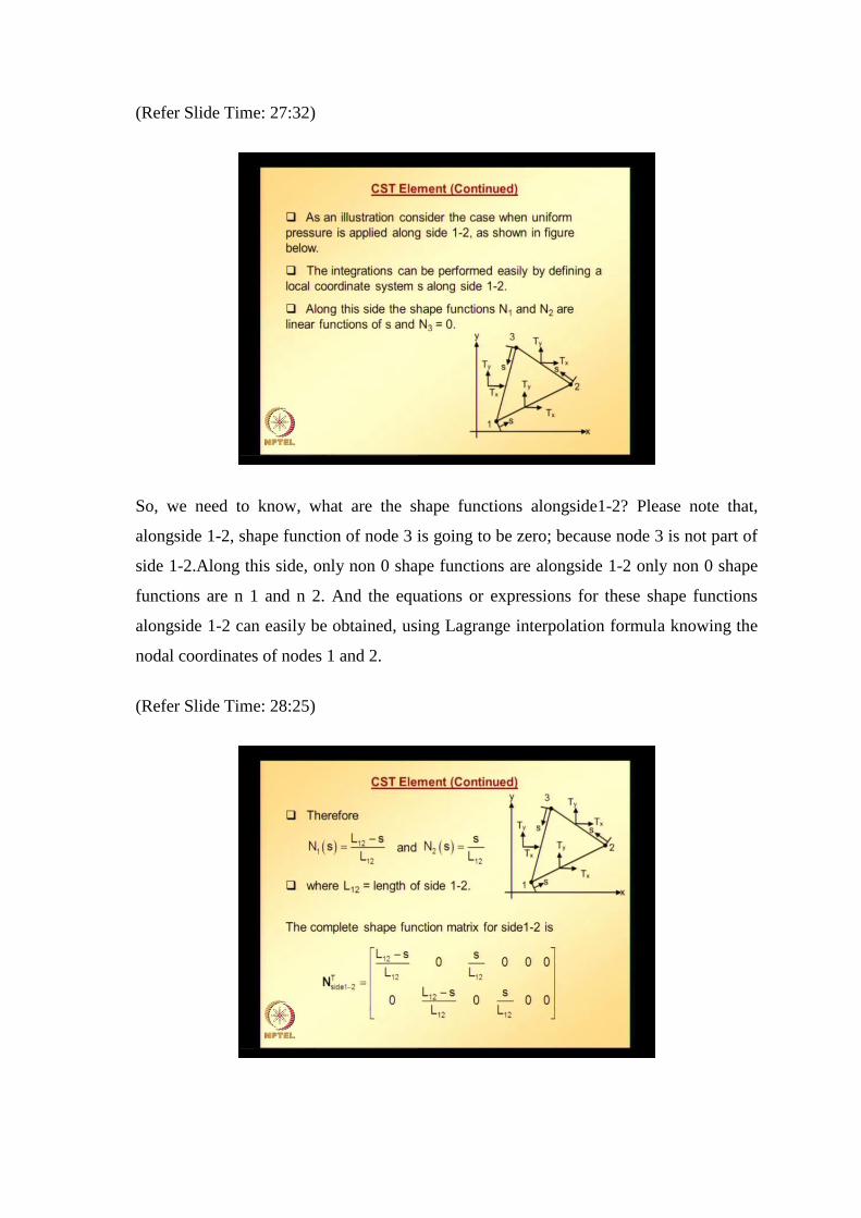
So, we need to know, what are the shape functions alongside1-2? Please note that,
alongside 1-2, shape function of node 3 is going to be zero; because node 3 is not part of
side 1-2.Along this side, only non 0 shape functions are alongside 1-2 only non 0 shape
functions are n 1 and n 2. And the equations or expressions for these shape functions
alongside 1-2 can easily be obtained, using Lagrange interpolation formula knowing the
nodal coordinates of nodes 1 and 2.
(Refer Slide Time: 28:25)
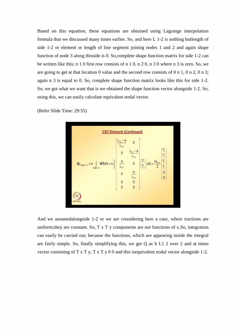
Based on this equation, these equations are obtained using Lagrange interpolation
formula that we discussed many times earlier. So, and here L 1-2 is nothing butlength of
side 1-2 or element or length of line segment joining nodes 1 and 2 and again shape
function of node 3 along thisside is 0. So,complete shape function matrix for side 1-2 can
be written like this; n 1 0 first row consists of n 1 0, n 2 0, n 3 0 where n 3 is zero. So, we
are going to get at that location 0 value and the second row consists of 0 n 1, 0 n 2, 0 n 3;
again n 3 is equal to 0. So, complete shape function matrix looks like this for side 1-2.
So, we got what we want that is we obtained the shape function vector alongside 1-2. So,
using this, we can easily calculate equivalent nodal vector.
(Refer Slide Time: 29:55)
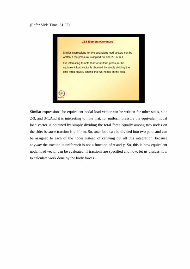
And we assumedalongside 1-2 or we are considering here a case, where tractions are
uniform;they are constant. So, T x T y components are not functions of x.So, integration
can easily be carried out; because the functions, which are appearing inside the integral
are fairly simple. So, finally simplifying this, we get Q as h L1 2 over 2 and at times
vector consisting of T x T y, T x T y 0 0 and this isequivalent nodal vector alongside 1-2.
(Refer Slide Time: 31:02)
Similar expressions for equivalent nodal load vector can be written for other sides, side
2-3, and 3-1.And it is interesting to note that, for uniform pressure the equivalent nodal
load vector is obtained by simply dividing the total force equally among two nodes on
the side; because traction is uniform. So, total load can be divided into two parts and can
be assigned to each of the nodes.Instead of carrying out all this integration, because
anyway the traction is uniform;it is not a function of x and y. So, this is how equivalent
nodal load vector can be evaluated, if tractions are specified and now, let us discuss how
to calculate work done by the body forces.
(Refer Slide Time: 32:21)
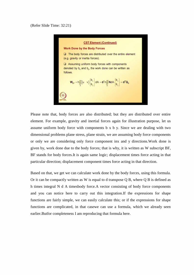
Please note that, body forces are also distributed; but they are distributed over entire
element. For example, gravity and inertial forces again for illustration purpose, let us
assume uniform body force with components b x b y. Since we are dealing with two
dimensional problems plane stress, plane strain, we are assuming body force components
or only we are considering only force component inx and y directions.Work done is
given by, work done due to the body forces; that is why, it is written as W subscript BF,
BF stands for body forces.It is again same logic; displacement times force acting in that
particular direction; displacement component times force acting in that direction.
Based on that, we get we can calculate work done by the body forces, using this formula.
Or it can be compactly written as W is equal to d transpose Q B, where Q B is defined as
h times integral N d A timesbody force.A vector consisting of body force components
and you can notice here to carry out this integration.If the expressions for shape
functions are fairly simple, we can easily calculate this; or if the expressions for shape
functions are complicated, in that casewe can use a formula, which we already seen
earlier.Butfor completeness I am reproducing that formula here.
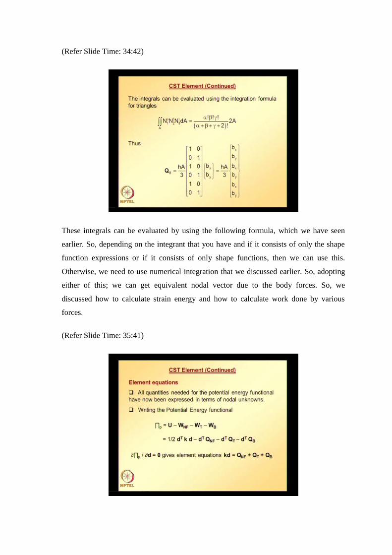
(Refer Slide Time: 34:42)
These integrals can be evaluated by using the following formula, which we have seen
earlier. So, depending on the integrant that you have and if it consists of only the shape
function expressions or if it consists of only shape functions, then we can use this.
Otherwise, we need to use numerical integration that we discussed earlier. So, adopting
either of this; we can get equivalent nodal vector due to the body forces. So, we
discussed how to calculate strain energy and how to calculate work done by various
forces.
(Refer Slide Time: 35:41)
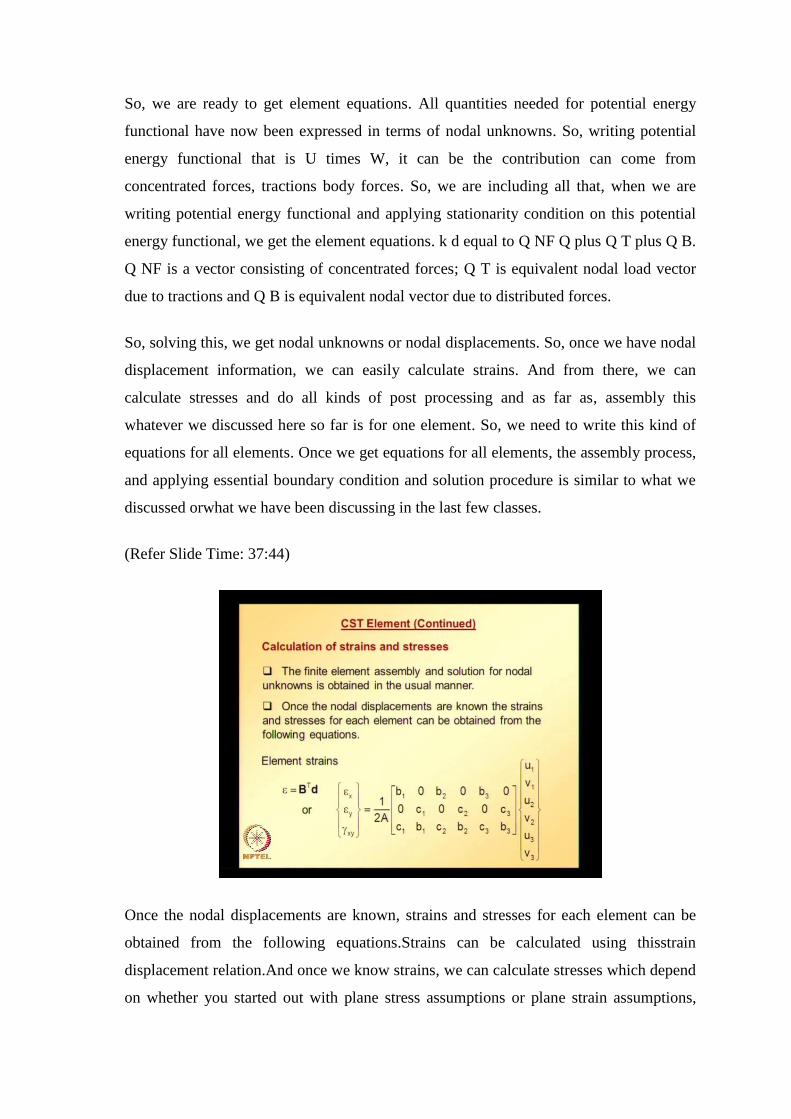
So, we are ready to get element equations. All quantities needed for potential energy
functional have now been expressed in terms of nodal unknowns. So, writing potential
energy functional that is U times W, it can be the contribution can come from
concentrated forces, tractions body forces. So, we are including all that, when we are
writing potential energy functional and applying stationarity condition on this potential
energy functional, we get the element equations. k d equal to Q NF Q plus Q T plus Q B.
Q NF is a vector consisting of concentrated forces; Q T is equivalent nodal load vector
due to tractions and Q B is equivalent nodal vector due to distributed forces.
So, solving this, we get nodal unknowns or nodal displacements. So, once we have nodal
displacement information, we can easily calculate strains. And from there, we can
calculate stresses and do all kinds of post processing and as far as, assembly this
whatever we discussed here so far is for one element. So, we need to write this kind of
equations for all elements. Once we get equations for all elements, the assembly process,
and applying essential boundary condition and solution procedure is similar to what we
discussed orwhat we have been discussing in the last few classes.
(Refer Slide Time: 37:44)
Once the nodal displacements are known, strains and stresses for each element can be
obtained from the following equations.Strains can be calculated using thisstrain
displacement relation.And once we know strains, we can calculate stresses which depend
on whether you started out with plane stress assumptions or plane strain assumptions,
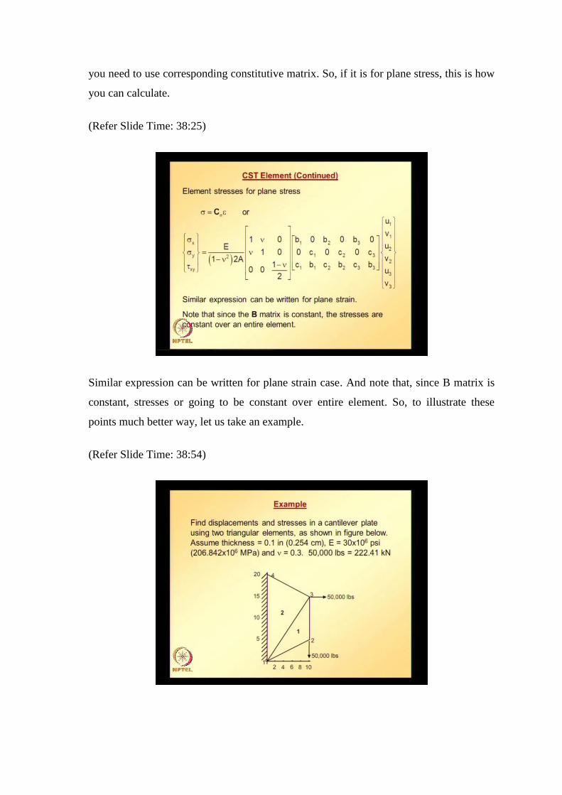
you need to use corresponding constitutive matrix. So, if it is for plane stress, this is how
you can calculate.
(Refer Slide Time: 38:25)
Similar expression can be written for plane strain case. And note that, since B matrix is
constant, stresses or going to be constant over entire element. So, to illustrate these
points much better way, let us take an example.
(Refer Slide Time: 38:54)
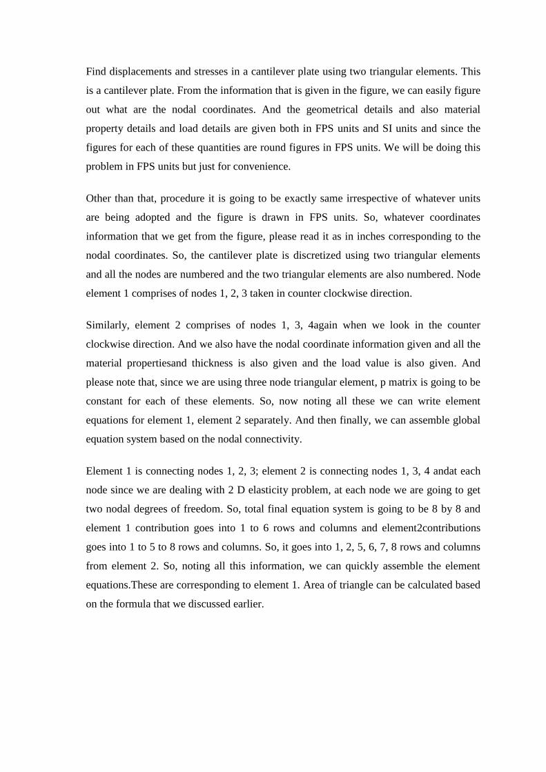
Find displacements and stresses in a cantilever plate using two triangular elements. This
is a cantilever plate. From the information that is given in the figure, we can easily figure
out what are the nodal coordinates. And the geometrical details and also material
property details and load details are given both in FPS units and SI units and since the
figures for each of these quantities are round figures in FPS units. We will be doing this
problem in FPS units but just for convenience.
Other than that, procedure it is going to be exactly same irrespective of whatever units
are being adopted and the figure is drawn in FPS units. So, whatever coordinates
information that we get from the figure, please read it as in inches corresponding to the
nodal coordinates. So, the cantilever plate is discretized using two triangular elements
and all the nodes are numbered and the two triangular elements are also numbered. Node
element 1 comprises of nodes 1, 2, 3 taken in counter clockwise direction.
Similarly, element 2 comprises of nodes 1, 3, 4again when we look in the counter
clockwise direction. And we also have the nodal coordinate information given and all the
material propertiesand thickness is also given and the load value is also given. And
please note that, since we are using three node triangular element, p matrix is going to be
constant for each of these elements. So, now noting all these we can write element
equations for element 1, element 2 separately. And then finally, we can assemble global
equation system based on the nodal connectivity.
Element 1 is connecting nodes 1, 2, 3; element 2 is connecting nodes 1, 3, 4 andat each
node since we are dealing with 2 D elasticity problem, at each node we are going to get
two nodal degrees of freedom. So, total final equation system is going to be 8 by 8 and
element 1 contribution goes into 1 to 6 rows and columns and element2contributions
goes into 1 to 5 to 8 rows and columns. So, it goes into 1, 2, 5, 6, 7, 8 rows and columns
from element 2. So, noting all this information, we can quickly assemble the element
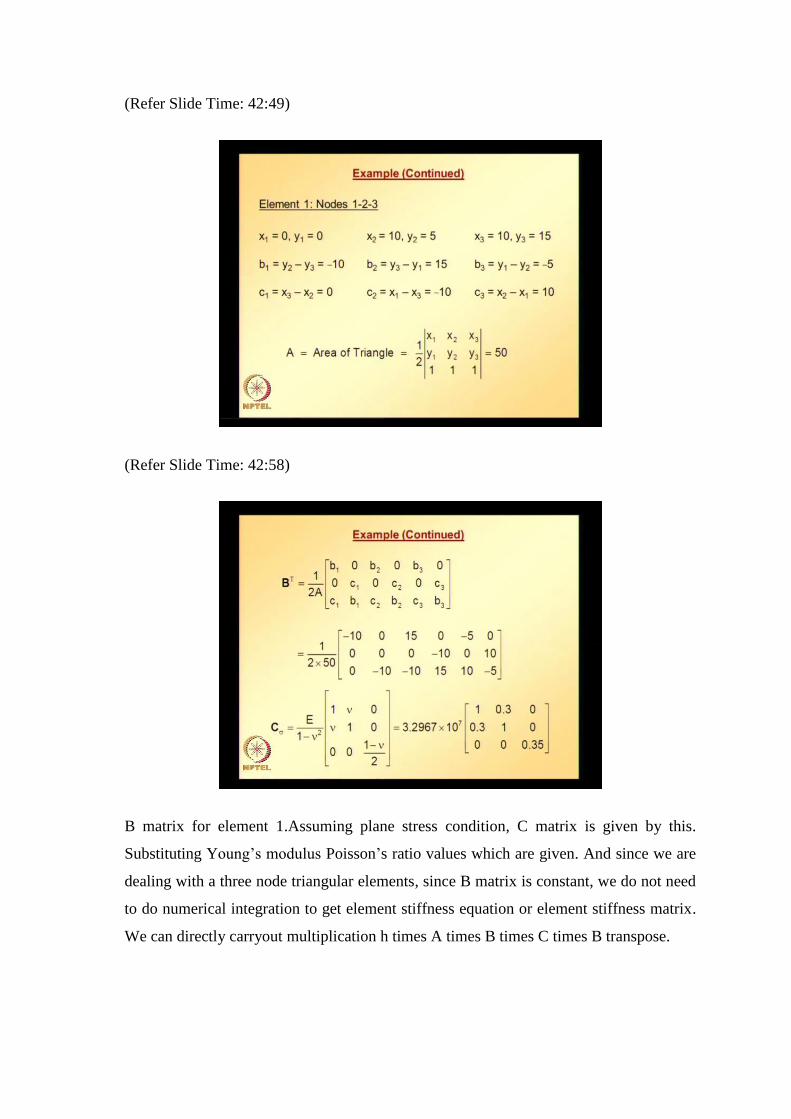
equations.These are corresponding to element 1. Area of triangle can be calculated based
on the formula that we discussed earlier.
(Refer Slide Time: 42:49)
(Refer Slide Time: 42:58)
B matrix for element 1.Assuming plane stress condition, C matrix is given by this.
Substituting Young’s modulus Poisson’s ratio values which are given. And since we are
dealing with a three node triangular elements, since B matrix is constant, we do not need
to do numerical integration to get element stiffness equation or element stiffness matrix.
We can directly carryout multiplication h times A times B times C times B transpose.
(Refer Slide Time: 43:55)
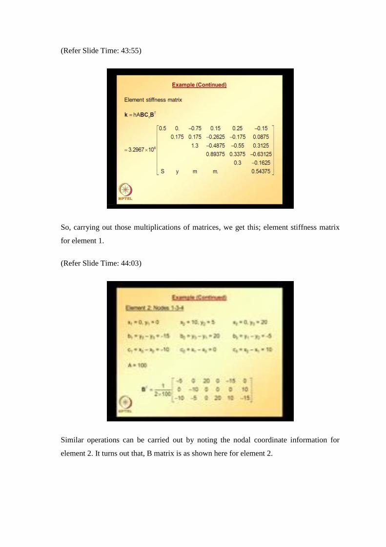
So, carrying out those multiplications of matrices, we get this; element stiffness matrix
for element 1.
(Refer Slide Time: 44:03)
Similar operations can be carried out by noting the nodal coordinate information for
element 2. It turns out that, B matrix is as shown here for element 2.
(Refer Slide Time: 44:22)
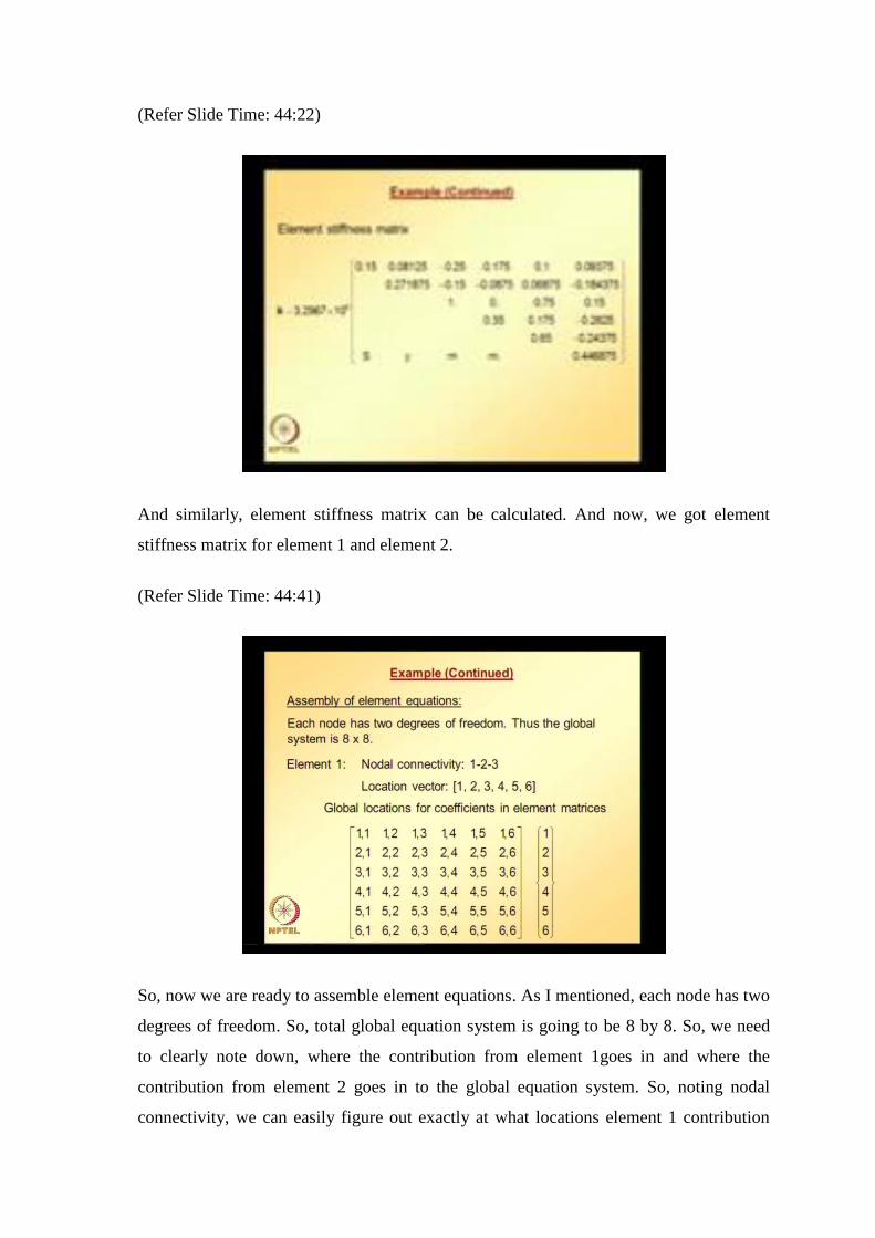
And similarly, element stiffness matrix can be calculated. And now, we got element
stiffness matrix for element 1 and element 2.
(Refer Slide Time: 44:41)
So, now we are ready to assemble element equations. As I mentioned, each node has two
degrees of freedom. So, total global equation system is going to be 8 by 8. So, we need
to clearly note down, where the contribution from element 1goes in and where the
contribution from element 2 goes in to the global equation system. So, noting nodal
connectivity, we can easily figure out exactly at what locations element 1 contribution

goes in, which is shown in location vector. Once we have this information, global
locations for coefficients in element matrices can be written or can be noted down in this
manner. This information helps us to assemble the global equation system. So, this is for
element 1.
(Refer Slide Time: 45:42)
Similarly, for element 2 nodal connectivity, corresponding location, vector global
locations for coefficients in element matrices. So, this matrix gives us global locations
for element 2. So, using this information, we can assemble element equations and noting
essential boundary condition,the global equations are as follows.
(Refer Slide Time: 46:14)
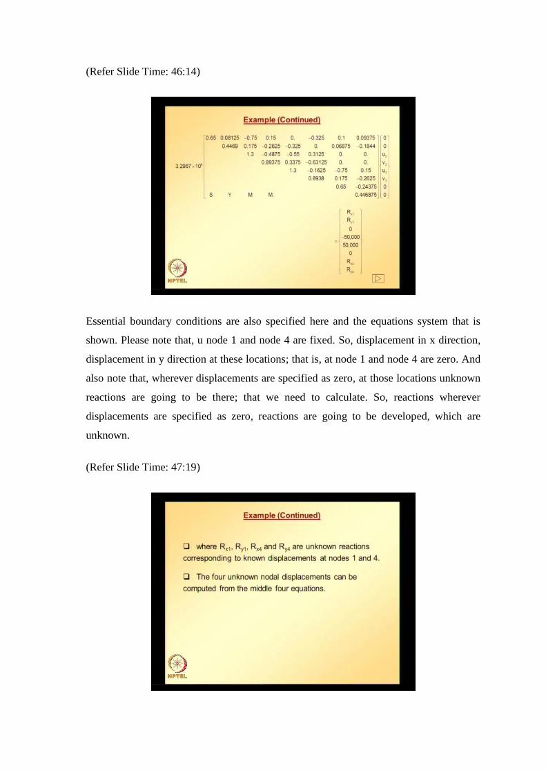
Essential boundary conditions are also specified here and the equations system that is
shown. Please note that, u node 1 and node 4 are fixed. So, displacement in x direction,
displacement in y direction at these locations; that is, at node 1 and node 4 are zero. And
also note that, wherever displacements are specified as zero, at those locations unknown
reactions are going to be there; that we need to calculate. So, reactions wherever
displacements are specified as zero, reactions are going to be developed, which are
unknown.
(Refer Slide Time: 47:19)
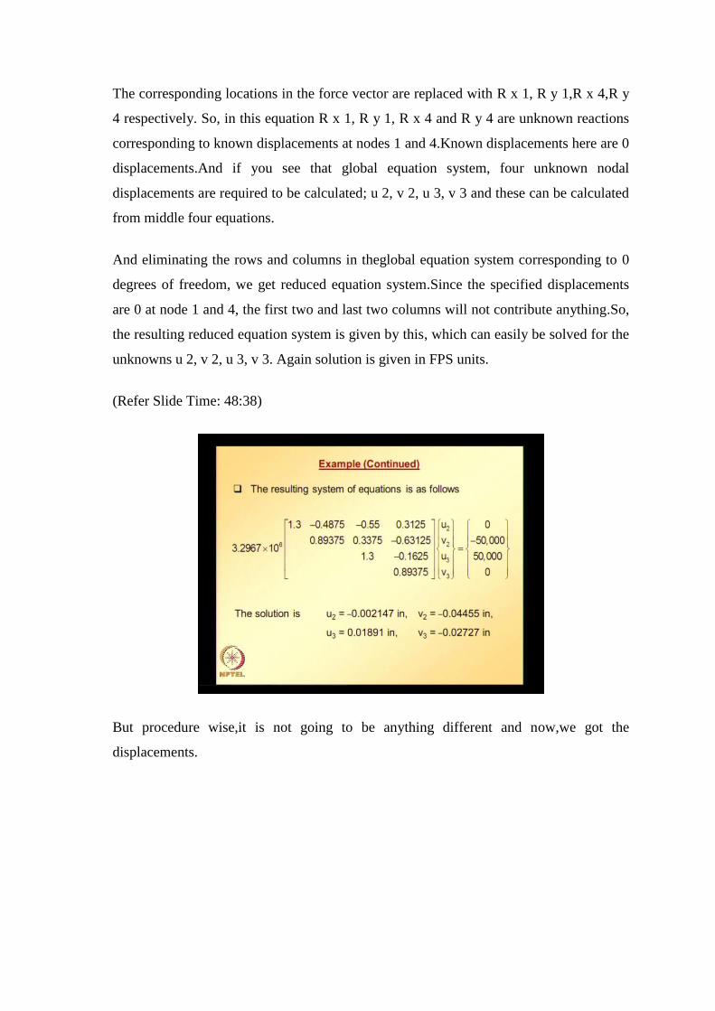
The corresponding locations in the force vector are replaced with R x 1, R y 1,R x 4,R y
4 respectively. So, in this equation R x 1, R y 1, R x 4 and R y 4 are unknown reactions
corresponding to known displacements at nodes 1 and 4.Known displacements here are 0
displacements.And if you see that global equation system, four unknown nodal
displacements are required to be calculated; u 2, v 2, u 3, v 3 and these can be calculated
from middle four equations.
And eliminating the rows and columns in theglobal equation system corresponding to 0
degrees of freedom, we get reduced equation system.Since the specified displacements
are 0 at node 1 and 4, the first two and last two columns will not contribute anything.So,
the resulting reduced equation system is given by this, which can easily be solved for the
unknowns u 2, v 2, u 3, v 3. Again solution is given in FPS units.
(Refer Slide Time: 48:38)
But procedure wise,it is not going to be anything different and now,we got the
displacements.
(Refer Slide Time: 48:48)
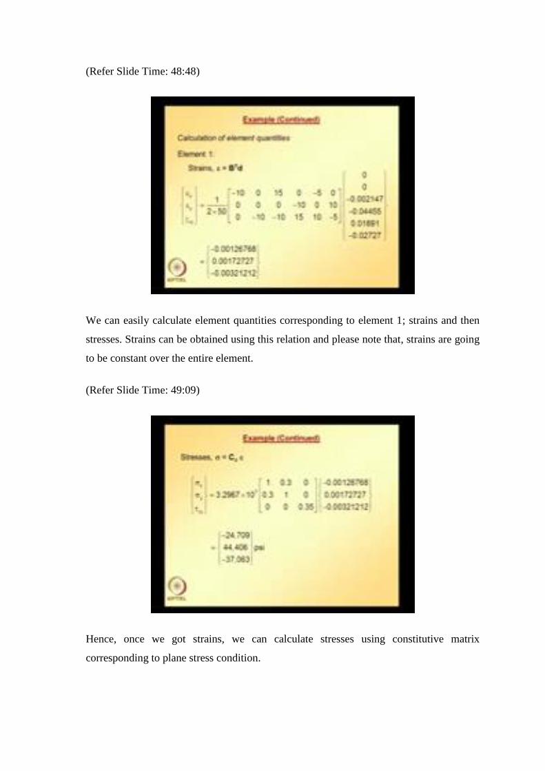
We can easily calculate element quantities corresponding to element 1; strains and then
stresses. Strains can be obtained using this relation and please note that, strains are going
to be constant over the entire element.
(Refer Slide Time: 49:09)
Hence, once we got strains, we can calculate stresses using constitutive matrix
corresponding to plane stress condition.
(Refer Slide Time: 49:25)
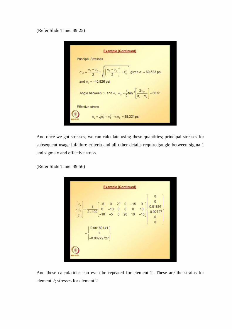
And once we got stresses, we can calculate using these quantities; principal stresses for
subsequent usage infailure criteria and all other details required;angle between sigma 1
and sigma x and effective stress.
(Refer Slide Time: 49:56)
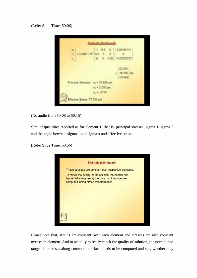
And these calculations can even be repeated for element 2. These are the strains for
element 2; stresses for element 2.
(Refer Slide Time: 50:06)
(No audio from 50:08 to 50:15)
Similar quantities reported as for element 1; that is, principal stresses, sigma 1, sigma 2
and the angle between sigma 1 and sigma x and effective stress.
(Refer Slide Time: 50:56)
Please note that, strains are constant over each element and stresses are also constant
over each element. And to actually to really check the quality of solution, the normal and
tangential stresses along common interface needs to be computed and see, whether they
are matching or not. What I mean by that iswe need to calculate these components using
stress transformation.
(Refer Slide Time: 51:08)
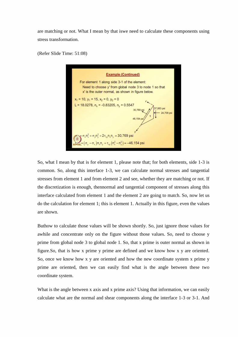
So, what I mean by that is for element 1, please note that; for both elements, side 1-3 is
common. So, along this interface 1-3, we can calculate normal stresses and tangential
stresses from element 1 and from element 2 and see, whether they are matching or not. If
the discretization is enough, thennormal and tangential component of stresses along this
interface calculated from element 1 and the element 2 are going to match. So, now let us
do the calculation for element 1; this is element 1. Actually in this figure, even the values
are shown.
Buthow to calculate those values will be shown shortly. So, just ignore those values for
awhile and concentrate only on the figure without those values. So, need to choose y
prime from global node 3 to global node 1. So, that x prime is outer normal as shown in
figure.So, that is how x prime y prime are defined and we know how x y are oriented.
So, once we know how x y are oriented and how the new coordinate system x prime y
prime are oriented, then we can easily find what is the angle between these two
coordinate system.
What is the angle between x axis and x prime axis? Using that information, we can easily
calculate what are the normal and shear components along the interface 1-3 or 3-1. And
for that, we require to note down what are the coordinates. we need to note down or we
need to know, what is the element length, line segment length connecting nodes 1 and
3.So,for that we required to note down, what are the coordinates of node 3. Node 3
coordinates are denoted with x 1, y 1 and node 1 coordinates are denoted with x 2, y 2.
And here for calculation purpose, node 3 is taken as first node and node 1 is taken as
second node. And from that, we can easily calculate what is the length and also we can
calculate, what are the direction cosines of outer normal alongside 3-1. And once we
have that information, we can easily calculate sigma x prime and tau x prime y prime
using these relations. So, this is what I am emphasizing that, these values of sigma x
prime tau x prime y prime values calculated from element 1 should match with element
2.Let us see, whether they match or not.
(Refer Slide Time: 54:25)
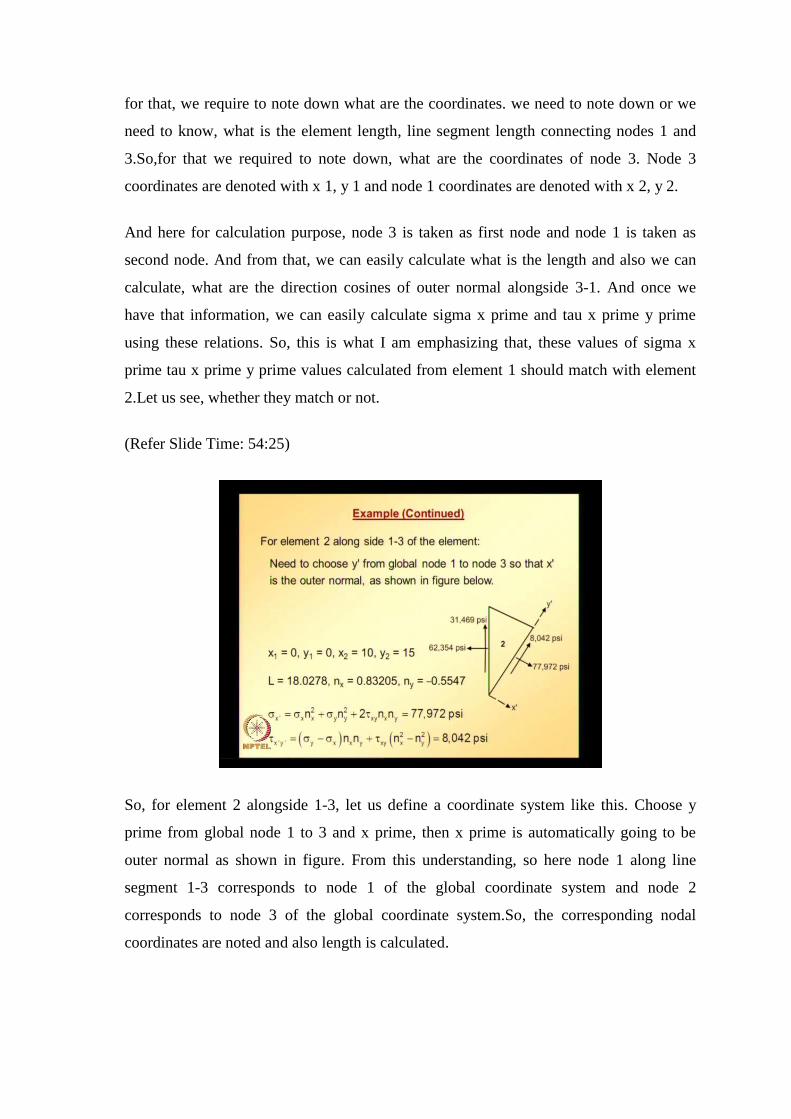
So, for element 2 alongside 1-3, let us define a coordinate system like this. Choose y
prime from global node 1 to 3 and x prime, then x prime is automatically going to be
outer normal as shown in figure. From this understanding, so here node 1 along line
segment 1-3 corresponds to node 1 of the global coordinate system and node 2
corresponds to node 3 of the global coordinate system.So, the corresponding nodal
coordinates are noted and also length is calculated.
Once we have this, we can calculate, what are the outer normal or direction cosines of
outer normal for this particular edge 1-3. Once we have this information, we can easily
calculate sigma x prime tau x prime y prime using these relations. So, we calculated
sigma x prime tau x prime y prime for both elements along the interface 1-3.So, we need
to see whether these values match or not. So, all these values are put side by side to see
whether they are matching or not.
(Refer Slide Time: 55:42)
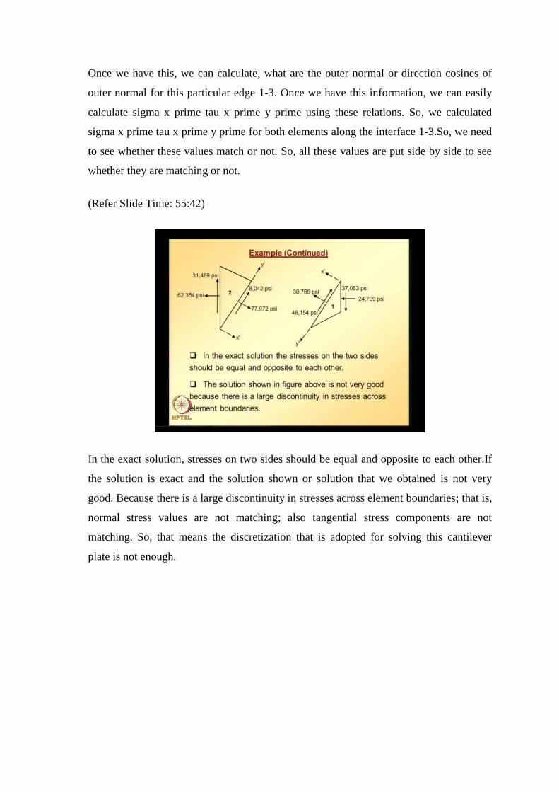
In the exact solution, stresses on two sides should be equal and opposite to each other.If
the solution is exact and the solution shown or solution that we obtained is not very
good. Because there is a large discontinuity in stresses across element boundaries; that is,
normal stress values are not matching; also tangential stress components are not
matching. So, that means the discretization that is adopted for solving this cantilever
plate is not enough.

(Refer Slide Time: 56:24)
With only two elements, mesh is very coarse, and we obviously cannot expect very good
results. As we increase the number of elements, the discontinuity in stresses should
reduce. Soand when if we really want increase the number of elements, then we cannot
do that using hand calculations; we need to automate this. So, this is about a three node
triangular element for solving plane stress, plane strain problems. And in the next class,
we will be looking at four node quadrilateral element.