Embed Size (px)
Citation preview
Finite Element Analysis of Suction BucketFoundations in Sand Subjected to CyclicLoading
Ingerid Elisabeth Rolstad Jahren
Civil and Environmental Engineering
Supervisor: Hans Petter Jostad, IBM
Department of Civil and Environmental Engineering
Submission date: June 2018
Norwegian University of Science and Technology

i
Preface
This is a master thesis written in the spring of 2018 as the final part of my M.Sc. degree in
Civil and Environmental Engineering at the Norwegian University of Science and Technology
(NTNU) in Trondheim. The thesis is a part of the master’s programme in Geotechnical Engi-
neering at the department of Civil and Environmental Engineering. The thesis has been carried
out in a cooperation with the Norwegian Geotechnical Institute (NGI), which also proposed the
thesis.
Trondheim, 2018-06-10
Ingerid Rolstad Jahren


iii
Acknowledgement
I would like to express my gratitude to my academic supervisor Adjunct Prof. Hans Petter Jostad,
NGI, who provided great insight and expertise throughout the thesis work. His interest and
enthusiasm for the topic in addition to great knowledge is truly inspiring.
I also thank members of the staff at the Geotechnical Division at NTNU for kindly sharing their
wisdom during my years as a student at NTNU.
Finally, thank you to all my fellow students for valuable discussions and support.
I.R.J.

v
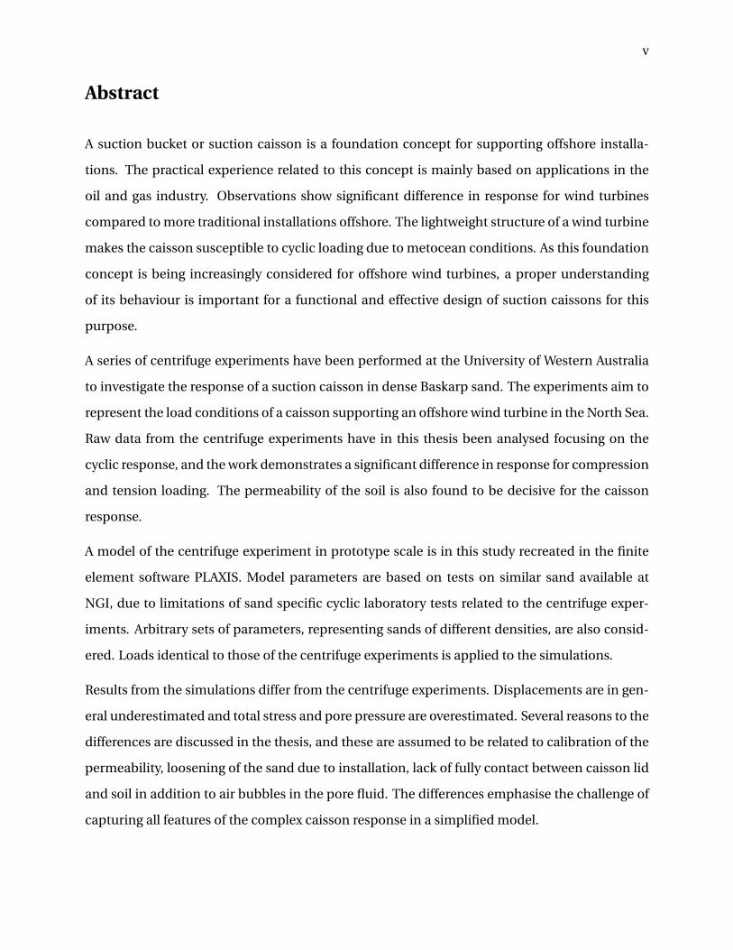
Abstract
A suction bucket or suction caisson is a foundation concept for supporting offshore installa-
tions. The practical experience related to this concept is mainly based on applications in the
oil and gas industry. Observations show significant difference in response for wind turbines
compared to more traditional installations offshore. The lightweight structure of a wind turbine
makes the caisson susceptible to cyclic loading due to metocean conditions. As this foundation
concept is being increasingly considered for offshore wind turbines, a proper understanding
of its behaviour is important for a functional and effective design of suction caissons for this
purpose.
A series of centrifuge experiments have been performed at the University of Western Australia
to investigate the response of a suction caisson in dense Baskarp sand. The experiments aim to
represent the load conditions of a caisson supporting an offshore wind turbine in the North Sea.
Raw data from the centrifuge experiments have in this thesis been analysed focusing on the
cyclic response, and the work demonstrates a significant difference in response for compression
and tension loading. The permeability of the soil is also found to be decisive for the caisson
response.
A model of the centrifuge experiment in prototype scale is in this study recreated in the finite
element software PLAXIS. Model parameters are based on tests on similar sand available at
NGI, due to limitations of sand specific cyclic laboratory tests related to the centrifuge exper-
iments. Arbitrary sets of parameters, representing sands of different densities, are also consid-
ered. Loads identical to those of the centrifuge experiments is applied to the simulations.
Results from the simulations differ from the centrifuge experiments. Displacements are in gen-
eral underestimated and total stress and pore pressure are overestimated. Several reasons to the
differences are discussed in the thesis, and these are assumed to be related to calibration of the
permeability, loosening of the sand due to installation, lack of fully contact between caisson lid
and soil in addition to air bubbles in the pore fluid. The differences emphasise the challenge of
capturing all features of the complex caisson response in a simplified model.

vii
Sammendrag
Bøttefundament eller sugeanker er et fundamenteringskonsept for offshore-installasjoner. Den
praktiske erfaringen tilknyttet dette konseptet er i hovedsak basert på anvendelser i olje- og
gassektoren. Undersøkelser viser en betydelig forskjell i oppførsel for vindturbiner sammen-
lignet med mer tradisjonelle installasjoner offshore. Den lette vindmøllekonstruksjonen gjør
bøttefundamentet sårbart for syklisk last fra vind, bølger og havstrømmer. Dette fundamenter-
ingskonseptet blir i økende grad vurdert for offshore vindmøller, og en god forståelse av dets
oppførsel er viktig for en funksjonell og effektiv utforming av bøttefundament til dette formålet.
En rekke sentrifugeforsøk er utført ved University of Western Australia for å analysere oppførse-
len til et bøttefundamet plassert i tettpakket Baskarp-sand. Forsøkene streber etter å gjenskape
lastforholdene for en offshore vindmølle plassert på toppen av et fundament i Nordsjøen. Rå-
data fra forsøkene er i denne avhandling analysert med fokus på syklisk respons, og arbei-
det viser en betydelig forskjell i respons avhengig av strekk- og trykkbelastning. Resultater fra
forsøkene viser også at permeabiliteten i sanden er avgjørende for oppførselen til bøttefunda-
mentet.
En modell av sentrifugeforsøkene i prototypeskala er i forbindelse med dette studiet laget i
finite element-programmet PLAXIS. Sandparametre er basert på tester av tilsvarende materi-
ale tilgjengelig ved NGI, da slike type tester ikke er gjennomført i forbindelse med sentrifuge-
forsøkene. Et sett av materialer med ulike densitet er også undersøkt. Lasttilfeller identisk til
sentrifugeforsøkene er benyttet i simuleringene.
Resultater fra simuleringene viser avvik fra sentrifugetestene. Forskyvningen er generelt under-
estimert og total- og poretrykk er overestimert. Oppgaven diskuterer mulige årsaker til avviket,
og disse er antatt å være tilknyttet kalibrering av permeabilitet, oppløsning av sand som følge
av installasjon, mangel på full kontakt mellom fundamentlokk og jord samt luftbobler i pore-
vannet. Avviket understreker utfordringen med å fange opp alle egenskapene i den komplekse
fundamentoppførselen i en forenklet modell.

Contents
Preface . . . . . . . . . . . . . . . . . . . . . . . . . . . . . . . . . . . . . . . . . . . . . . . . i
Acknowledgement . . . . . . . . . . . . . . . . . . . . . . . . . . . . . . . . . . . . . . . . . iii
Abstract . . . . . . . . . . . . . . . . . . . . . . . . . . . . . . . . . . . . . . . . . . . . . . . . v
Sammendrag . . . . . . . . . . . . . . . . . . . . . . . . . . . . . . . . . . . . . . . . . . . . vii
List of Symbols xi
1 Introduction 1
1.1 Background . . . . . . . . . . . . . . . . . . . . . . . . . . . . . . . . . . . . . . . . . . 1
1.2 Objectives . . . . . . . . . . . . . . . . . . . . . . . . . . . . . . . . . . . . . . . . . . . 3
1.3 Limitations . . . . . . . . . . . . . . . . . . . . . . . . . . . . . . . . . . . . . . . . . . . 3
1.4 Scientific Approach . . . . . . . . . . . . . . . . . . . . . . . . . . . . . . . . . . . . . . 4
1.5 Outline of the Thesis . . . . . . . . . . . . . . . . . . . . . . . . . . . . . . . . . . . . . 4
2 Behaviour of Suction Caissons for Offshore Wind Turbines 5
2.1 Installation and Applications of Suction Caissons . . . . . . . . . . . . . . . . . . . . 5
2.1.1 Installation . . . . . . . . . . . . . . . . . . . . . . . . . . . . . . . . . . . . . . . 5
2.1.2 Applications . . . . . . . . . . . . . . . . . . . . . . . . . . . . . . . . . . . . . . 6
2.2 Limiting Conditions for Offshore Wind Turbines . . . . . . . . . . . . . . . . . . . . . 7
3 Cyclic Behaviour of Sand and the HCA Model 11
3.1 Cyclic Behaviour of Sand . . . . . . . . . . . . . . . . . . . . . . . . . . . . . . . . . . . 11
3.1.1 Monotonic Loading . . . . . . . . . . . . . . . . . . . . . . . . . . . . . . . . . 12
3.1.2 Cyclic Loading . . . . . . . . . . . . . . . . . . . . . . . . . . . . . . . . . . . . . 13
ix
x CONTENTS
3.2 High-Cycle Accumulation Model . . . . . . . . . . . . . . . . . . . . . . . . . . . . . . 14
3.2.1 Explicit Calculation Strategy . . . . . . . . . . . . . . . . . . . . . . . . . . . . 14
3.2.2 Parameters in the HCA Model . . . . . . . . . . . . . . . . . . . . . . . . . . . 15
4 Centrifuge Experiments of Suction Caissons in Sand 19
4.1 Measurements and Equipment . . . . . . . . . . . . . . . . . . . . . . . . . . . . . . . 19
4.2 Cyclic Loading . . . . . . . . . . . . . . . . . . . . . . . . . . . . . . . . . . . . . . . . . 20
4.3 Material Parameters . . . . . . . . . . . . . . . . . . . . . . . . . . . . . . . . . . . . . 22
4.4 Extraction Resistance . . . . . . . . . . . . . . . . . . . . . . . . . . . . . . . . . . . . . 24
5 Recalculation of Centrifuge Experiments in PLAXIS 25
5.1 Structure of the Model . . . . . . . . . . . . . . . . . . . . . . . . . . . . . . . . . . . . 25
5.1.1 Finite Element Mesh . . . . . . . . . . . . . . . . . . . . . . . . . . . . . . . . . 27
5.1.2 Variations of the Model . . . . . . . . . . . . . . . . . . . . . . . . . . . . . . . 29
5.1.3 Calculation Types and Loading . . . . . . . . . . . . . . . . . . . . . . . . . . . 30
5.2 Adaption of Parameters . . . . . . . . . . . . . . . . . . . . . . . . . . . . . . . . . . . 31
5.2.1 Stiffness Parameters for the Hardening Soil Model . . . . . . . . . . . . . . . 31
5.2.2 The Hardening Soil model with Small-Strain Stiffness . . . . . . . . . . . . . 35
5.2.3 Extraction Resistance . . . . . . . . . . . . . . . . . . . . . . . . . . . . . . . . 36
5.2.4 Consolidation Parameters . . . . . . . . . . . . . . . . . . . . . . . . . . . . . . 36
5.2.5 Overview of Input Parameters and Description of Other Materials . . . . . . 38
6 Results 39
6.1 Centrifuge Experiments . . . . . . . . . . . . . . . . . . . . . . . . . . . . . . . . . . . 39
6.1.1 Displacement . . . . . . . . . . . . . . . . . . . . . . . . . . . . . . . . . . . . . 41
6.1.2 Total Stress and Pore Pressure . . . . . . . . . . . . . . . . . . . . . . . . . . . . 45
6.1.3 Amplitudes of Cyclic Applied Load, Displacement, Total Stress and Pore
Pressure . . . . . . . . . . . . . . . . . . . . . . . . . . . . . . . . . . . . . . . . 45
6.2 Recalculation Using PLAXIS . . . . . . . . . . . . . . . . . . . . . . . . . . . . . . . . . 50
6.3 Miscellaneous Variations for PLAXIS Simulations . . . . . . . . . . . . . . . . . . . . 59
6.3.1 Replaced Soil Tip . . . . . . . . . . . . . . . . . . . . . . . . . . . . . . . . . . . 59
6.3.2 Variation in Permeability . . . . . . . . . . . . . . . . . . . . . . . . . . . . . . 60
CONTENTS xi
6.3.3 Water Pocket Beneath Caisson Lid . . . . . . . . . . . . . . . . . . . . . . . . . 61
7 Discussion 63
7.1 Discussion on Cyclic Peak Amplitudes . . . . . . . . . . . . . . . . . . . . . . . . . . . 63
7.1.1 Centrifuge Experiments . . . . . . . . . . . . . . . . . . . . . . . . . . . . . . . 63
7.1.2 PLAXIS Simulations . . . . . . . . . . . . . . . . . . . . . . . . . . . . . . . . . 67
7.2 Type of Behaviour and Material . . . . . . . . . . . . . . . . . . . . . . . . . . . . . . . 69
7.2.1 Drained and Undrained Behaviour . . . . . . . . . . . . . . . . . . . . . . . . 69
7.2.2 Materials . . . . . . . . . . . . . . . . . . . . . . . . . . . . . . . . . . . . . . . . 70
7.2.3 Time Histories and Phase Changes . . . . . . . . . . . . . . . . . . . . . . . . . 72
7.3 Reasons for Differences in Centrifuge Experiments and PLAXIS Simulations . . . . 73
7.3.1 Loosening of Soil Due to Installation . . . . . . . . . . . . . . . . . . . . . . . 74
7.3.2 Consolidation and Redistribution of Forces . . . . . . . . . . . . . . . . . . . 74
7.3.3 Gap Between Caisson Lid and Soil . . . . . . . . . . . . . . . . . . . . . . . . . 76
7.3.4 Air Bubbles in Pore Fluid . . . . . . . . . . . . . . . . . . . . . . . . . . . . . . 77
7.3.5 Summary of Reasons for Difference in Centrifuge Experiments and PLAXIS
Simulations . . . . . . . . . . . . . . . . . . . . . . . . . . . . . . . . . . . . . . 78
7.4 Relevance of Centrifuge Experiments and Use of Data from External Sources . . . . 78
8 Conclusion and Recommendations for Further Work 81
8.1 Summary and Conclusion . . . . . . . . . . . . . . . . . . . . . . . . . . . . . . . . . . 81
8.2 Recommendations for Further Work . . . . . . . . . . . . . . . . . . . . . . . . . . . . 82
List of Figures 88
List of Tables 90
Bibliography 90

List of Symbols
N drainage path ratio
Y av normalised stress ratio
1 second order identity tensor
ε trend of strain
εacc rate of strain accumulation
εpl plastic strain rate
σ′ trend of effective stress
σ′∗ deviatoric part of effective stress
E elastic stiffness tensor
m direction of strain accumulation
εacc intensity of strain accumulation
εaccq deviatoric strain accumulation rate
εaccv volumetric strain accumulation rate
fN function for cyclic preloading (HCA model)
f AN , f B
N parts A (structural accumulation) and B (basic rate), respectively, of the function for
cyclic preloading (HCA model)
ε strain
xiii
xiv CONTENTS
εampl strain amplitude
εamplr e f reference strain amplitude
εav average strain
εa axial strain
εh , ε′h horizontal stress and horizontal effective stress
εv , ε′v vertical stress and vertical effective stress
η stress ratio
γs shear strain
γsat saturated unit weight
γunsat unsaturated unit weight
ν Poisson’s ratio
νs shear wave velocity
φ′ friction angle
φ′p peak friction angle
φ′cv ultimate value friction angle
ψ dilatancy angle
ρ soil density
σ, σ′ total and effective stress
σ1, σ′1 major in-plane principal total and effective stress
σ3, σ′3 minor in-plane total and effective stress
σa axial stress
σh ,σ′h horizontal total stress and horizontal effective stress
σr radial stress
CONTENTS xv
σv ,σ′v vertical total stress and vertical effective stress
τ shear strength
c cohesion
Cu uniformity coefficient
Cv coefficient of consolidation
Campl HCA model parameter, function fampl
Ce HCA model parameter, function fe
CN 1,CN 2,CN 3 membrane penetration correction factors
Cp HCA model parameter, function fp
CY HCA model parameter, function fY
d10 grain diameter of 10 % passing
d60 grain diameter of 60 % passing
Dr relative density
E stiffness
e void ratio
E50 average stiffness
E r e f50 reference average stiffness
emax ,emi n maximum and minimum pore ratio, respectively
Eoed oedometer modulus
E r e foed reference oedometer modulus
er e f reference void ratio
Eur unloading / reloading stiffness
E r e fur reference unloading / reloading stiffness
xvi CONTENTS
fπ function for polarization changes (HCA model)
fampl amplitude function (HCA model)
fe void ratio function (HCA model)
fp pressure function (HCA model)
fY stress ratio function (HCA model)
G shear stiffness modulus
g A historiotropic variable (HCA-model)
g0 initial shear stiffness modulus
h drainage path
k permeability
K0 initial earth pressure at rest
M inclination of critical state line
p effective mean pressure
pav average effective mean pressure
pr e f reference effective mean pressure
q deviatoric stress
q av average deviatoric stress
Ri nter strength reduction factor
Tv time factor
εampl strain amplitude
→ Euclidean norm
m power for stress-level dependency of stiffness
N number of cycles

CONTENTS xvii
t time
u pore pressure

Chapter 1
Introduction
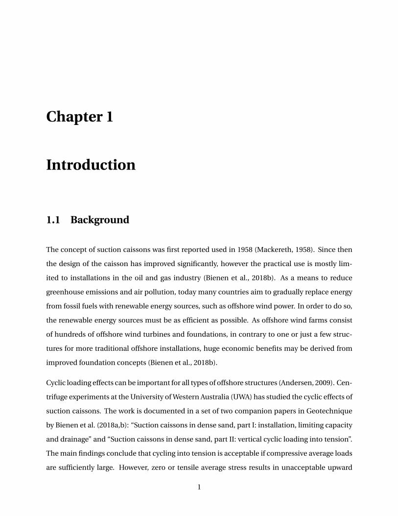
1.1 Background
The concept of suction caissons was first reported used in 1958 (Mackereth, 1958). Since then
the design of the caisson has improved significantly, however the practical use is mostly lim-
ited to installations in the oil and gas industry (Bienen et al., 2018b). As a means to reduce
greenhouse emissions and air pollution, today many countries aim to gradually replace energy
from fossil fuels with renewable energy sources, such as offshore wind power. In order to do so,
the renewable energy sources must be as efficient as possible. As offshore wind farms consist
of hundreds of offshore wind turbines and foundations, in contrary to one or just a few struc-
tures for more traditional offshore installations, huge economic benefits may be derived from
improved foundation concepts (Bienen et al., 2018b).
Cyclic loading effects can be important for all types of offshore structures (Andersen, 2009). Cen-
trifuge experiments at the University of Western Australia (UWA) has studied the cyclic effects of
suction caissons. The work is documented in a set of two companion papers in Geotechnique
by Bienen et al. (2018a,b): “Suction caissons in dense sand, part I: installation, limiting capacity
and drainage” and “Suction caissons in dense sand, part II: vertical cyclic loading into tension”.
The main findings conclude that cycling into tension is acceptable if compressive average loads
are sufficiently large. However, zero or tensile average stress results in unacceptable upward
1
2 CHAPTER 1. INTRODUCTION
displacements. The study also investigates the importance of drainage conditions for the cais-
son response and highlights the complexity of caisson behaviour. These studies have provided
valuable insight into the caisson response. However, further studies should aim to understand
the relationship between applied cyclic loading, displacements and stress response in addition
to drainage and stiffness of the caisson response.
Water saturated sand will during cyclic loading accumulate displacements or pore pressure, or
both. The effect of accumulation is accounted for in a high-cycle accumulation (HCA) model for
sand described by Wichtmann (2005) and Niemunis et al. (2005). Displacements of suction cais-
sons supporting offshore wind turbines cannot be tolerated due to strict in-service rotational
limits (Peire et al., 2009). Additionally, only a small range of frequency is suitable for design as
the eigenfrequencies of a single blade and the rotor should be avoided (Bienen et al., 2018b).
As the accumulation influences the displacement, and thus the rotation of the caisson, in ad-
dition to the soil stiffness, which is decisive for the eigenfrequency of the system, the effects of
accumulation must be properly taken into account in design.
Problem Formulation
The thesis focuses on cyclic behaviour of suction caissons and centrifuge experiments per-
formed at the UWA, which is recalculated using PLAXIS. A deeper understanding of the cyclic
response of suction caissons supporting offshore wind turbines is essential for improved design.
The problem formulations are stated as followed:
1. How is cyclic loading effecting the response of suction caissons supporting offshore wind
turbines?
2. How does the simulations based on the centrifuge experiments from the UWA manage to
capture the features of the suction caisson response?
1.2. OBJECTIVES 3
1.2 Objectives
The aim of the thesis is to investigate the cyclic response of suction caissons in water saturated
dense sand by recalculating a centrifuge experiment at the UWA.
By using theory on the cyclic response of suction caissons supporting offshore wind turbines
and the HCA model, the main objectives of this thesis are:
1. Examination of the results from suction caisson experiments performed in a centrifuge at
the UWA.
2. Recalculation of the experiments using the finite element program PLAXIS.
1.3 Limitations
The thesis concentrates on centrifuge experiments performed at the UWA. The raw data used
to evaluate the experiments contain several different cyclic loading histories. In this thesis, only
one of the loading history events is examined. The difference in pore fluid viscosity for this
loading cycle is still included in this study. However, no information about initial total stresses
or pore pressures are given in the raw data files, which complicates and limits the possibility to
recreate the response of the caisson in the simulations.
Due to the complexity of the caisson behaviour and limitations in time, the examination of the
HCA model is narrowed down to a literature survey. This means that no simulations or calcula-
tions are performed with respect to the HCA model. The recalculation of the centrifuge experi-
ments are therefore exclusively performed with a standard material model, which response may
differ from typical cyclic behaviour.
4 CHAPTER 1. INTRODUCTION
1.4 Scientific Approach
A literature survey has been carried out to develop an understanding of the behaviour of suction
caissons for offshore wind turbines. This includes investigation of cyclic behaviour of sand and
the HCA model.
Results from centrifuge experiments of a suction caisson in dense sand performed at the UWA
have been examined to further understand the behaviour of suction caissons. The examination
of the experiments also provides important data for simulations in PLAXIS.
The centrifuge experiments are recalculated in PLAXIS in order to interpret the cyclic response
of the suction caisson.
1.5 Outline of the Thesis
The remaining chapters of the thesis are structured as follows:
Chapter 2 gives an introduction to suction caissons and its behaviour in connection to offshore
wind turbines.
Chapter 3 describes cyclic behaviour of sand and introduces the high-cycle accumulation model.
Chapter 4 explains how the centrifuge experiments are performed.
Chapter 5 explains the method used for recalculating the centrifuge experiments in PLAXIS.
Chapter 6 presents the results from the centrifuge experiments and PLAXIS simulations.
Chapter 7 gives a discussion on the results from the centrifuge experiments and PLAXIS simu-
lations.
Chapter 8 presents a final conclusion, summary and recommendations for further work.
Chapter 2
Behaviour of Suction Caissons for Offshore
Wind Turbines
A suction caisson is best illustrated as an upturned bucket which is lowered into the seabed.
The installation process is vital for its functionality, but once the bucket is properly installed, it
forms a solid foundation for offshore structures. The interest for the foundation concept seems
still to be rising, also for offshore wind turbines. However, compared to more traditional offshore
structures, other design criteria and limiting conditions apply for offshore wind turbines.
2.1 Installation and Applications of Suction Caissons
2.1.1 Installation
Suction caissons are more frequently being considered for offshore foundations due to their
ease of installation. Shorter installation time, shallower final penetration depth and installation
without pile driving make this foundation concept preferred on several occasions rather than
more traditional foundation alternatives such as offshore pile foundations (Jia, 2018).
The installation process can be divided into two phases; self-weight penetration and suction
installation. The foundation is lowered to the seafloor, and initial penetration of the skirts into
5
6 CHAPTER 2. BEHAVIOUR OF SUCTION CAISSONS FOR OFFSHORE WIND TURBINES
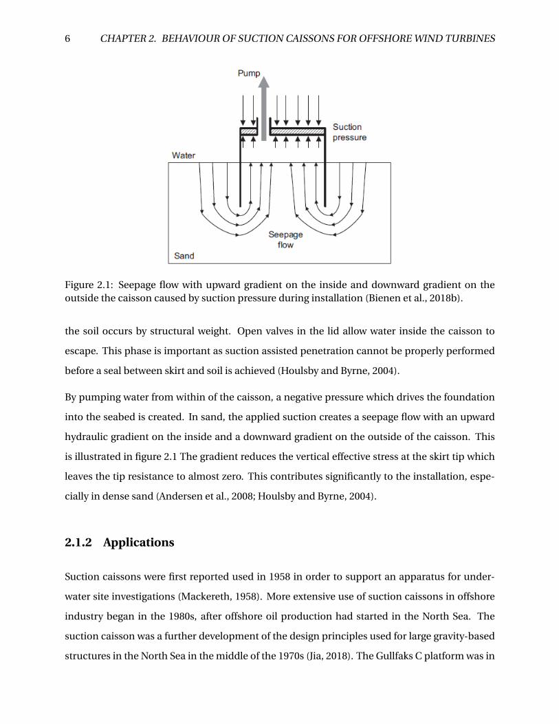
Figure 2.1: Seepage flow with upward gradient on the inside and downward gradient on theoutside the caisson caused by suction pressure during installation (Bienen et al., 2018b).
the soil occurs by structural weight. Open valves in the lid allow water inside the caisson to
escape. This phase is important as suction assisted penetration cannot be properly performed
before a seal between skirt and soil is achieved (Houlsby and Byrne, 2004).
By pumping water from within of the caisson, a negative pressure which drives the foundation
into the seabed is created. In sand, the applied suction creates a seepage flow with an upward
hydraulic gradient on the inside and a downward gradient on the outside of the caisson. This
is illustrated in figure 2.1 The gradient reduces the vertical effective stress at the skirt tip which
leaves the tip resistance to almost zero. This contributes significantly to the installation, espe-
cially in dense sand (Andersen et al., 2008; Houlsby and Byrne, 2004).
2.1.2 Applications
Suction caissons were first reported used in 1958 in order to support an apparatus for under-
water site investigations (Mackereth, 1958). More extensive use of suction caissons in offshore
industry began in the 1980s, after offshore oil production had started in the North Sea. The
suction caisson was a further development of the design principles used for large gravity-based
structures in the North Sea in the middle of the 1970s (Jia, 2018). The Gullfaks C platform was in
2.2. LIMITING CONDITIONS FOR OFFSHORE WIND TURBINES 7
1989 installed with 16-meter-large diameter suction caissons penetrating totally 22 meters into
the seabed (Tjelta et al., 1990). However, in 1999 the record-breaking Diana platform was in-
stalled at 1500 meters depth with a 30-meter-tall suction caisson of diameter 6.5 meters (Bybee
et al., 2001), and in 1994 Draupner E proved that suction caissons were not only applicable in
soft soils as the platform was installed in dense to very dense sand layers (Bye et al., 1995).
In recent years the usage of suction caissons as foundation for offshore wind turbines has been
studied, but the practical experience at full scale is still limited. However, at a test field in Fred-
erikshavn, Denmark, a prototype of a suction caisson supporting an offshore wind turbine was
installed on dense sand in 2002 (Ibsen, 2008). In addition monitored suction caissons have been
used for met masts at Horns Rev 2 and Dogger Bank (Tjelta, 2015), and at Borkum Riffgrund, Ger-
many, an offshore wind turbine is supported by suction caissons and connected to 126 different
sensors from the top of the structure to the suction caisson below seabed (Tjelta, 2015).
It is worth mentioning that structures in the gas and oil industry are typically a one-off installa-
tion where improvements in the installation process will have a limited beneficial effect. Wind
farms, however, can contain hundreds of wind turbines and may gain huge financial benefits
from better foundation design or alternative foundation concepts (Bienen et al., 2018b).
2.2 Limiting Conditions for Offshore Wind Turbines
Compared to the design of traditional structures in the gas and oil industry, offshore wind tur-
bines differ in many important ways. The allowed off-vertical tilt of the offshore wind turbine is
limited to 0.25◦ (Peire et al., 2009), which makes serviceability, rather than capacity, the critical
design factor. As deformation of the foundation is the main contributor to rotation of the off-
shore wind turbine, the effect of cyclic loading on accumulated settlement of the caissons must
be carefully considered (Bienen et al., 2018b).
The design of offshore wind turbines needs to avoid the eigenfrequency of both a single blade
and the rotor, which results in only a small range of target eigenfrequency. As the foundation
stiffness strongly impacts the eigenfrequency of the system, it is important to carefully study its
8 CHAPTER 2. BEHAVIOUR OF SUCTION CAISSONS FOR OFFSHORE WIND TURBINES
behaviour (Bienen et al., 2018b). The stiffness might be affected due to large number of applied
load cycles, and accumulation of stiffness should therefore be an important part of that study.
Changes in the soil stiffness over 25 years of design life for offshore wind turbines makes it very
complicated to choose a single stiffness to represent the foundation response in structural anal-
yses (Bienen et al., 2018a).
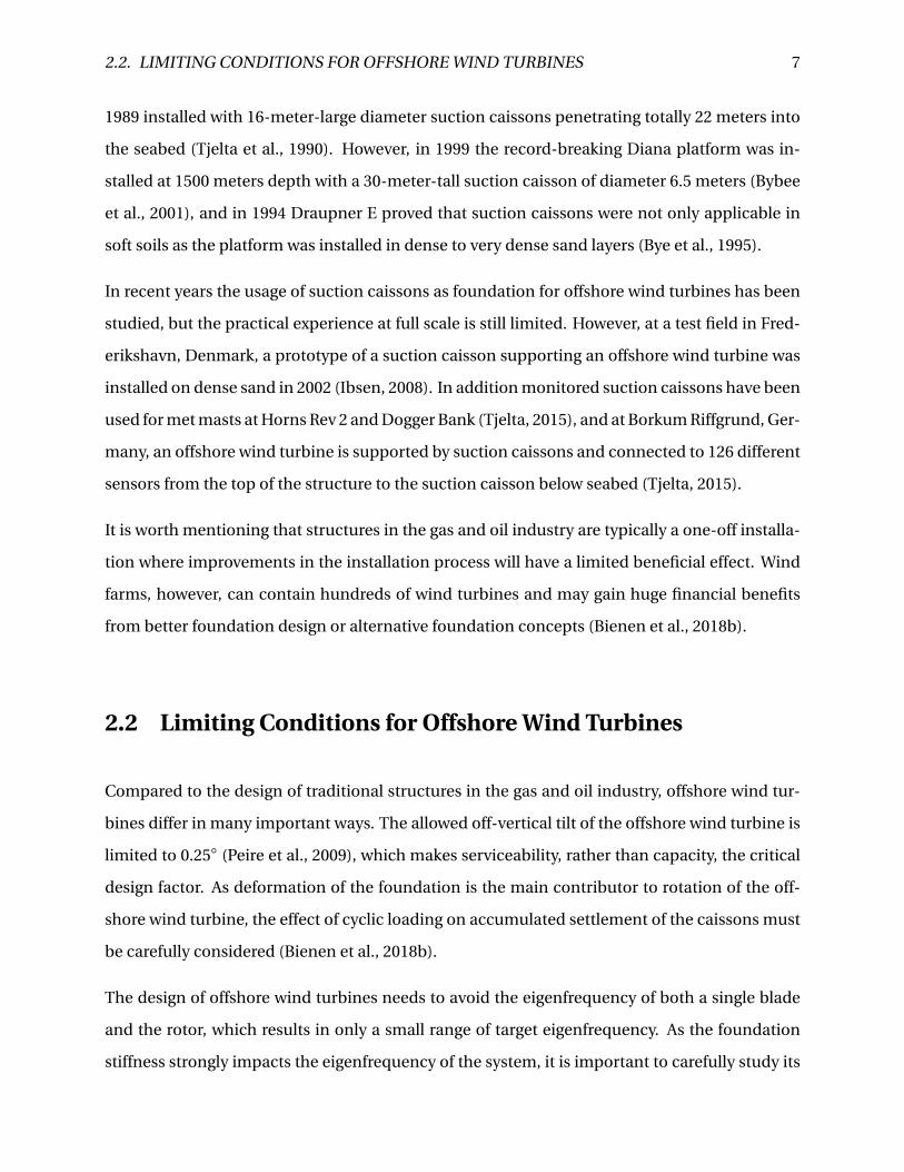
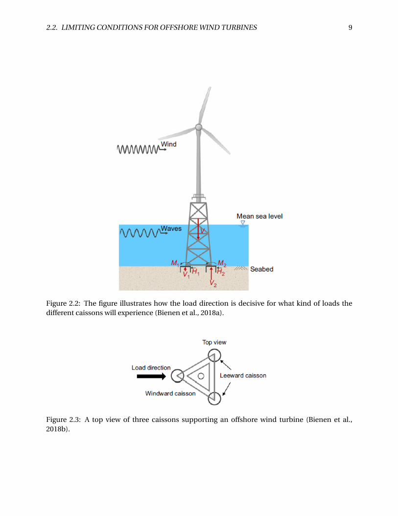
Offshore wind turbines are also much lighter and will experience bigger horizontal and mo-
ment loads compared to traditional offshore structures. The turbine superstructures can be
supported by one single caisson or a group of three or four caissons. For multi-caisson foun-
dation systems, each caisson will experience different loads depending on the metocean condi-
tions and the direction of loading, see figure 2.2 and 2.3. When subjected to wind loads, the lee-
ward caisson is heavily loaded, while the windward caisson is lightly loaded. The lightly loaded
caisson can be exposed to cyclic loading into tension, and might therefore be the limiting design
condition (Bienen et al., 2018b).
It is evident that upward permanent displacement must be avoided. When the caisson is pushed
down, the soil will become stronger and stiffer, and resistance against downward deformations
will become larger. This is not the case for upward displacement. When pulled upward the pen-
etration depth is reduced, the caisson’s lid might lose contact with the soil plug, the resistance
against further displacement becomes smaller and the structure may collapse. To protect struc-
tures against this type of displacement, the tensile loading has in general been limited to the
frictional capacity (Houlsby, 2016).
2.2. LIMITING CONDITIONS FOR OFFSHORE WIND TURBINES 9
Figure 2.2: The figure illustrates how the load direction is decisive for what kind of loads thedifferent caissons will experience (Bienen et al., 2018a).
Figure 2.3: A top view of three caissons supporting an offshore wind turbine (Bienen et al.,2018b).

Chapter 3
Cyclic Behaviour of Sand and the HCA Model
Offshore installations are typically exposed to cyclic loads due to wind and waves. In order to
fully understand the cyclic behaviour of suction caissons, it is important to study soil mechanics
relevant for this foundation concept. This chapter describes both the important soil features of
monotonic and cyclic loading. In addition, the main concept of the high-cycle accumulation
(HCA) model is examined.
3.1 Cyclic Behaviour of Sand
Cyclic loading may cause accumulation of pore pressure and deformation. This occurs not only
due to large strains, but also for large numbers of cycles with small strain-amplitudes. During
drained loading, every load cycle causes a small change in the soil structure which increases the
soil displacement. For undrained cyclic loading the pore pressure build-up reduces effective
stresses, and the soil stiffness and shear strength will therefore decrease. In extreme cases this
can cause soil liquefaction and loss of the overall stability (Niemunis et al., 2005).
Important soil mechanics applicable to suction caissons in sands are presented by Bye et al.
(1995). The essence from Bye’s paper is provided in this section (3.1).
11
12 CHAPTER 3. CYCLIC BEHAVIOUR OF SAND AND THE HCA MODEL
3.1.1 Monotonic Loading
The soil shear strength of saturated soil, τ, is given by the effective stress,σ′, and frictional angle,
φ′:
τ=σ′t anφ′ (3.1)
When a load is applied to the soil, it is carried by solid grains and pore water pressure. The rate
of applied loading determines the size of excess pore water pressure. Considering an idealised
elastic, non-dilatant soil, it will not experience any change in mean effective stress due to an
instantaneous change of load. However, the pore water pressure will change instantaneous,
and a non-isotropic stress increment will result in a change in shear stresses. Despite this, the
soil strength will not be affected.
Dissipation of the induced pore water pressure over time generates changes in effective stresses
and thus changes in the soil strength. With the passage of time, a compression load on bucket
foundation will cause the mean effective stress to increase, and hence the soil strength. Like-
wise, a tension load will lead to decrease in mean effective load and reduction of soil strength
with time. This is the reason why caution is necessary when designing offshore wind turbines
with respect to tensile loads, see section 2.2. Finally, when all induced pore pressure is fully
dissipated, the small contribution from friction on the skirt walls is the only resistance against
tensile loads.
The idealisation of elastic and non-dilatant soil are generally not applicable for real soils. Obser-
vations show that the soil either contract or dilate. Very dense sand, which is further examined,
will in general dilate and loose sand contracts. The phenomenon where neither contractancy
nor dilatancy occur, i.e. no volume change during shearing, is called "critical state" and takes
place for one particular mean stress and void ratio.
When water flow is insufficient, the expansion due to dilatant behaviour of soil is prevented by
the incompressible nature of water due to suction. In addition, the mean effective stress in-
creases and thus the shear strength. The true limiting strength is not reached until soil effective
stresses and density have changed so much that the critical state is achieved. The term “steady
3.1. CYCLIC BEHAVIOUR OF SAND 13
state” strength is used to describe the equivalent phenomenon limited to fully undrained be-
haviour. For this type of behaviour, the cavitation pressure must also limit the strength. This
is the level of vacuum pressure where water vaporises, and can occur due to a rapid change of
pressure.
3.1.2 Cyclic Loading
Bucket foundations are mainly subjected to cyclic loads. This type of loading results in another
very important mechanism; pore pressure accumulation. The soil matrix of all sands, even the
densest, will tend to contract during cyclic undrained loading and hence accumulate pore pres-
sure. This type of sand with very high bulk stiffness can generate huge pore pressures. However,
for dense sand to reach the same level of pore pressure accumulation as initially looser sand,
the amplitude of the load cycles must be larger and more numerous compared to lose sands.
In the extreme case “initial liquefaction” occurs when the pore pressure build-up reduces the
soil mean effective stress to zero, which consequently leads to a huge reduction in shear stiff-
ness. Very dense sands will, when sheared to large enough strains, recover the lost stiffness.
However, the permanent strains may be way larger than tolerated.
Cyclic loading may cause irreversible strains under conditions less extreme than initial liquefac-
tion. Soil particles tend to rearrange during repeated cyclic loading, even when the amplitude
is low. The connections between the soil grains may collapse and the contact area and tension
between the grains change. Even though these changes might be infinitesimal, the effect is no-
ticeable on the deformation after hundreds or thousands load cycles (Zhou and Chen, 2005).
This type of displacement as a result a large number of cycles is accumulated deformation.
14 CHAPTER 3. CYCLIC BEHAVIOUR OF SAND AND THE HCA MODEL
3.2 High-Cycle Accumulation Model
The purpose of high-cycle accumulation (HCA) models is to calculate settlements or stress re-
laxation in soils due to a combination of average loads and large numbers of small-strain cyclic
loads. The HCA model also takes the accumulation of pore pressure during cyclic loading of
water saturated sand under nearly undrained conditions into account (Wichtmann et al., 2010).
The HCA model described in detail by Niemunis et al. (2005) and (Wichtmann, 2005) is based
on the fundamental idea that an oscillating part and a trend part can describe the stress and
strain paths generated by high-cyclic loading. The main focus of the model is the trend part,
which is predicted by accumulation of strain, εacc , while the oscillating part is represented by
the strain amplitude, εampl . The cumulative trend can either consist of small residual strains
(pseudo-creep) or residual stresses (pseudo relaxation), and is related by the following formula:
σ′ = E : (ε− εacc − εpl ) (3.2)
where σ′ is the effective stress rate, E is the elastic stiffness tensor, ε is the rate of stain, εacc is
the accumulated strain rate and εpl is the rate of plastic strain. Compression is here defined as
positive, both for stress and strain. Note that when studying high cycles models the term “rate”
refers to the derivative with respect to number of cycles, N , and not time, t .
To estimate the accumulation due to high cyclic loads a combination of a special explicit calcu-
lation strategy, a HCA model and finite element analysis may be used.
3.2.1 Explicit Calculation Strategy
For low-cycle load problems, pure implicit calculation strategies such as elastoplastic multi-
surface models or endochronic models are normally used. However, these methods give numer-
ical errors when applied to large number of cycles (Niemunis et al., 2005). An explicit strategy
usable for high-cyclic loads calculate only a small number of cycles implicitly. The main part of
the cycles are calculated explicitly by calculating the accumulation of strain directly. A packet of
3.2. HIGH-CYCLE ACCUMULATION MODEL 15
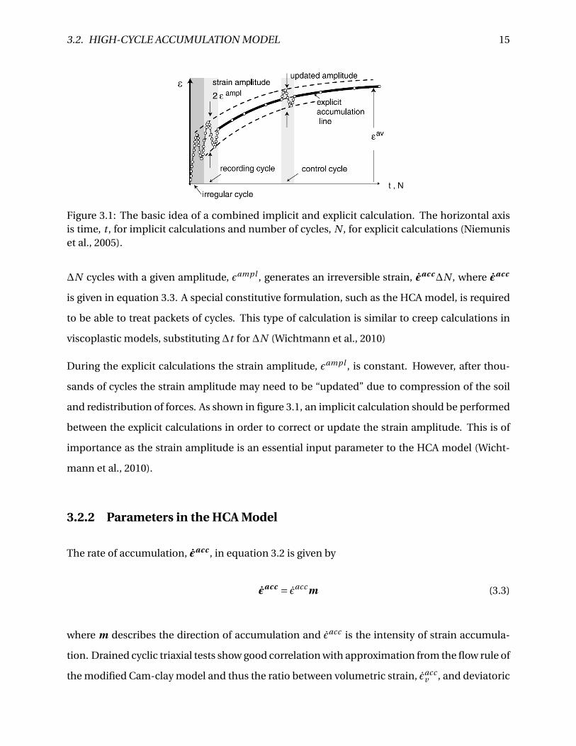
Figure 3.1: The basic idea of a combined implicit and explicit calculation. The horizontal axisis time, t , for implicit calculations and number of cycles, N , for explicit calculations (Niemuniset al., 2005).
∆N cycles with a given amplitude, εampl , generates an irreversible strain, εacc∆N , where εacc
is given in equation 3.3. A special constitutive formulation, such as the HCA model, is required
to be able to treat packets of cycles. This type of calculation is similar to creep calculations in
viscoplastic models, substituting ∆t for ∆N (Wichtmann et al., 2010)
During the explicit calculations the strain amplitude, εampl , is constant. However, after thou-
sands of cycles the strain amplitude may need to be “updated” due to compression of the soil
and redistribution of forces. As shown in figure 3.1, an implicit calculation should be performed
between the explicit calculations in order to correct or update the strain amplitude. This is of
importance as the strain amplitude is an essential input parameter to the HCA model (Wicht-
mann et al., 2010).
3.2.2 Parameters in the HCA Model
The rate of accumulation, εacc , in equation 3.2 is given by
εacc = εacc m (3.3)
where m describes the direction of accumulation and εacc is the intensity of strain accumula-
tion. Drained cyclic triaxial tests show good correlation with approximation from the flow rule of
the modified Cam-clay model and thus the ratio between volumetric strain, εaccv , and deviatoric
16 CHAPTER 3. CYCLIC BEHAVIOUR OF SAND AND THE HCA MODEL
strain, εaccq . As this approximation is used in the HCA-model, m is given as
m =[
1
3(p − q2
M 2p1+ 3
M 2σ′∗
]→(3.4)
where the subscript arrow indicate Euclidean norm, 1 is the second order identity tensor and
σ′∗ denotes the deviatoric part of the effective stresses. The effective mean pressure, p, and
deviatoric stress, q , are for drained triaxial tests given as p = (σ′1 +2σ′
3)/3 and q = σ′1 −σ′
3. The
inclination of the critical state line is M = 6si nφ3±si nφ .
The intensity of strain accumulation, εacc , is given by six independent functions, see equation
3.5, which account for different influencing parameters.
εacc = fampl fN fe fp fY fπ (3.5)
The effect of strain amplitude, εampl , is expressed by fampl , while fπ expresses the effect of polar-
isation. For constant polarisation fπ = 1. Increase of average stress ratio, η= q av
pav , and reduction
of mean pressure, pav , will cause εacc to increase, and this is predicted by the functions fp and
fY . Increasing void ratio, e, described by fe , results in increasing εacc . Cyclic preloading and its
dependency on εacc are captured by the function fN = f AN + f B
N . The preload is dependent on
number of cycles and their amplitude, and the model quantify this by
g A =∫
fampl f AN d N (3.6)
which is included in fN . The accumulation curves, εacc (N ), is proportional to fN = CN 1[ln(1+CN 2N )+CN 3N ] for cycles of constant amplitude.
A summary of functions and constants in addition to example values of constants for N = 105
cycles are given in table 3.1.
The parameters of the HCA model are described in more detail by Niemunis et al. (2005) and
Wichtmann (2005). Due to time limitations in the project period of the master thesis, the study
of the HCA-model is limited to this literature survey.
3.2. HIGH-CYCLE ACCUMULATION MODEL 17
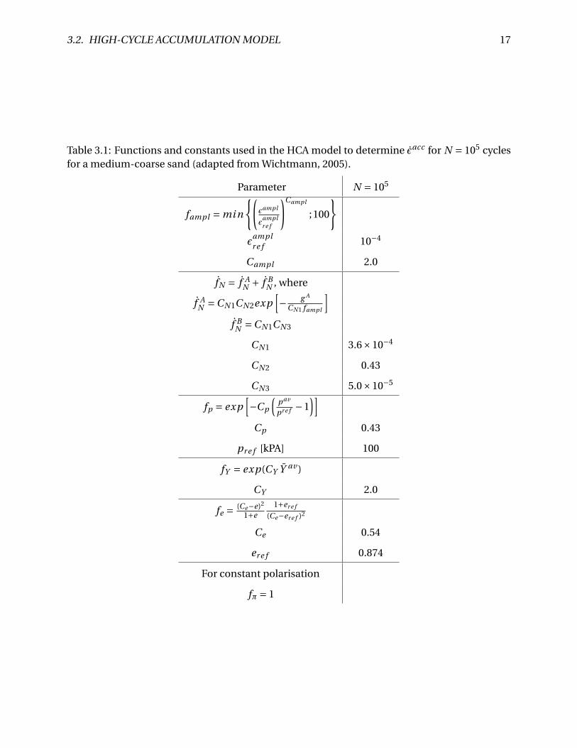
Table 3.1: Functions and constants used in the HCA model to determine εacc for N = 105 cyclesfor a medium-coarse sand (adapted from Wichtmann, 2005).
Parameter N = 105
fampl = mi n
{(εampl
εamplr e f
)Campl
;100
}ε
amplr e f 10−4
Campl 2.0
fN = f AN + f B
N , where
f AN =CN 1CN 2exp
[− g A
CN 1 fampl
]f B
N =CN 1CN 3
CN 1 3.6×10⁻⁴
CN 2 0.43
CN 3 5.0×10⁻⁵
fp = exp[−Cp
(pav
pr e f −1)]
Cp 0.43
pr e f [kPA] 100
fY = exp(CY Y av )
CY 2.0
fe = (Ce−e)2
1+e1+er e f
(Ce−er e f )2
Ce 0.54
er e f 0.874
For constant polarisation
fπ = 1

Chapter 4
Centrifuge Experiments of Suction Caissons
in Sand
To develop better insight into the cyclic behaviour of suction caissons in dense sand, a series
of centrifuge experiments are performed at the University of Western Australia (UWA), and de-
scribed in detail in a set of two companion papers in Geotechnique by Bienen et al. (2018a,b):
“Suction caissons in dense sand, part I: installation, limiting capacity and drainage” and “Suc-
tion caissons in dense sand, part II: vertical cyclic loading into tension”. A model caisson simu-
lates one of the three suction caissons supporting an offshore wind turbine on a jacket support
structure. The main focus of the research is on performance during installation, response to
cyclic loading and caisson extraction behaviour.
To achieve soil stresses similar those of the prototype, all tests are conducted in a beam cen-
trifuge at an acceleration of 100 g. The samples are composed of extremely dense Baskarp sand
and saturated with high viscosity pore fluid of 100 cSt or 660 cSt.
4.1 Measurements and Equipment
The model caisson made of aluminium with 40 mm skirt length, 0.5 mm skirt thickness and a
diameter of 80 mm is equivalent to a prototype caisson with 4 m skirt length, 50 mm skirt thick-
19
20 CHAPTER 4. CENTRIFUGE EXPERIMENTS OF SUCTION CAISSONS IN SAND
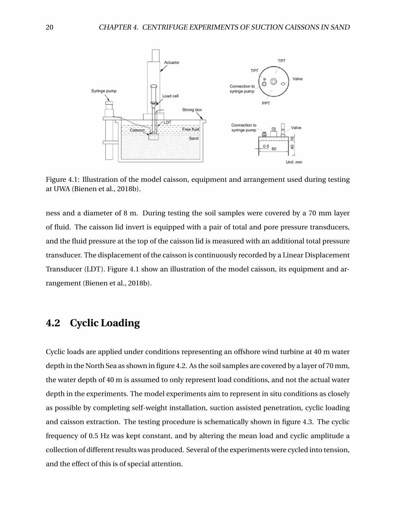
Figure 4.1: Illustration of the model caisson, equipment and arrangement used during testingat UWA (Bienen et al., 2018b).
ness and a diameter of 8 m. During testing the soil samples were covered by a 70 mm layer
of fluid. The caisson lid invert is equipped with a pair of total and pore pressure transducers,
and the fluid pressure at the top of the caisson lid is measured with an additional total pressure
transducer. The displacement of the caisson is continuously recorded by a Linear Displacement
Transducer (LDT). Figure 4.1 show an illustration of the model caisson, its equipment and ar-
rangement (Bienen et al., 2018b).
4.2 Cyclic Loading
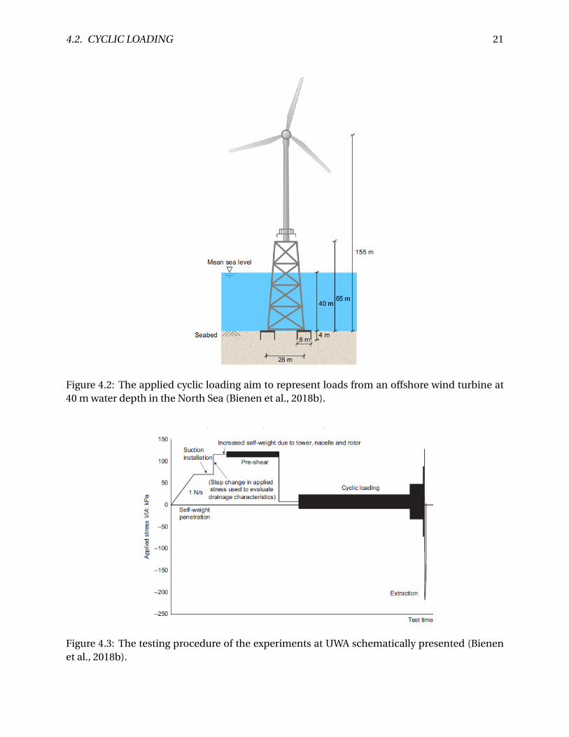
Cyclic loads are applied under conditions representing an offshore wind turbine at 40 m water
depth in the North Sea as shown in figure 4.2. As the soil samples are covered by a layer of 70 mm,
the water depth of 40 m is assumed to only represent load conditions, and not the actual water
depth in the experiments. The model experiments aim to represent in situ conditions as closely
as possible by completing self-weight installation, suction assisted penetration, cyclic loading
and caisson extraction. The testing procedure is schematically shown in figure 4.3. The cyclic
frequency of 0.5 Hz was kept constant, and by altering the mean load and cyclic amplitude a
collection of different results was produced. Several of the experiments were cycled into tension,
and the effect of this is of special attention.
4.2. CYCLIC LOADING 21
Figure 4.2: The applied cyclic loading aim to represent loads from an offshore wind turbine at40 m water depth in the North Sea (Bienen et al., 2018b).
Figure 4.3: The testing procedure of the experiments at UWA schematically presented (Bienenet al., 2018b).
22 CHAPTER 4. CENTRIFUGE EXPERIMENTS OF SUCTION CAISSONS IN SAND
4.3 Material Parameters
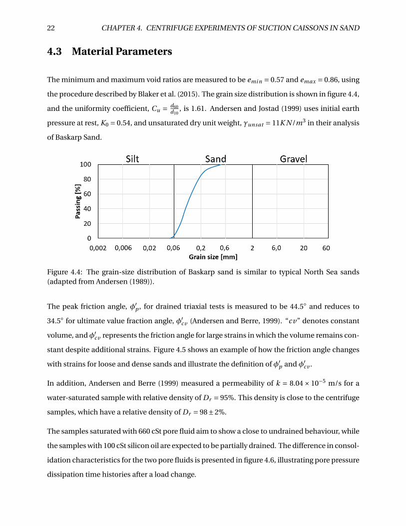
The minimum and maximum void ratios are measured to be emi n = 0.57 and emax = 0.86, using
the procedure described by Blaker et al. (2015). The grain size distribution is shown in figure 4.4,
and the uniformity coefficient, Cu = d60d10
, is 1.61. Andersen and Jostad (1999) uses initial earth
pressure at rest, K0 = 0.54, and unsaturated dry unit weight, γunsat = 11K N /m3 in their analysis
of Baskarp Sand.
Figure 4.4: The grain-size distribution of Baskarp sand is similar to typical North Sea sands(adapted from Andersen (1989)).
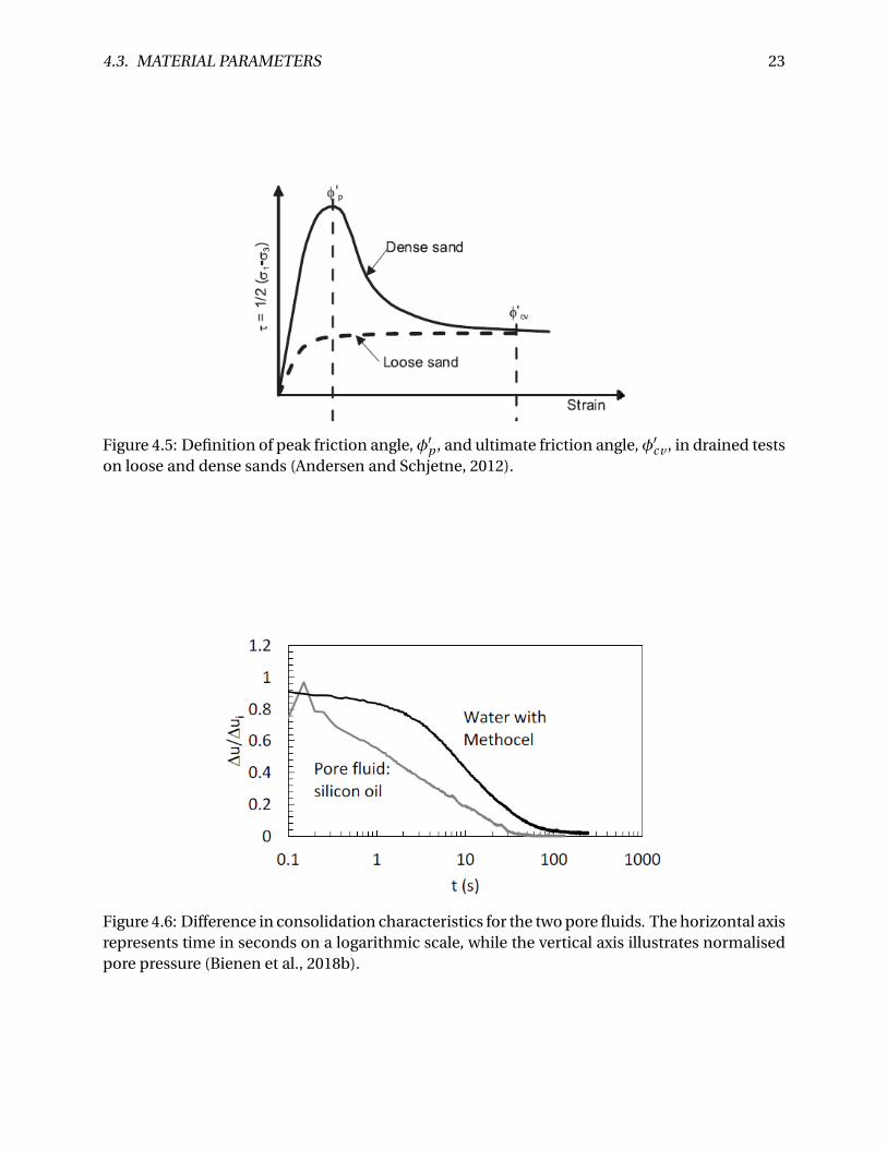
The peak friction angle, φ′p , for drained triaxial tests is measured to be 44.5◦ and reduces to
34.5◦ for ultimate value fraction angle, φ′cv (Andersen and Berre, 1999). “cv” denotes constant
volume, andφ′cv represents the friction angle for large strains in which the volume remains con-
stant despite additional strains. Figure 4.5 shows an example of how the friction angle changes
with strains for loose and dense sands and illustrate the definition of φ′p and φ′
cv .
In addition, Andersen and Berre (1999) measured a permeability of k = 8.04× 10⁻⁵ m/s for a
water-saturated sample with relative density of Dr = 95%. This density is close to the centrifuge
samples, which have a relative density of Dr = 98±2%.
The samples saturated with 660 cSt pore fluid aim to show a close to undrained behaviour, while
the samples with 100 cSt silicon oil are expected to be partially drained. The difference in consol-
idation characteristics for the two pore fluids is presented in figure 4.6, illustrating pore pressure
dissipation time histories after a load change.
4.3. MATERIAL PARAMETERS 23
Figure 4.5: Definition of peak friction angle, φ′p , and ultimate friction angle, φ′
cv , in drained testson loose and dense sands (Andersen and Schjetne, 2012).
Figure 4.6: Difference in consolidation characteristics for the two pore fluids. The horizontal axisrepresents time in seconds on a logarithmic scale, while the vertical axis illustrates normalisedpore pressure (Bienen et al., 2018b).
24 CHAPTER 4. CENTRIFUGE EXPERIMENTS OF SUCTION CAISSONS IN SAND
4.4 Extraction Resistance
To measure the pull-out capacity of the caisson, extraction has been conducted at a rate of
0.001 mm/s and 3 mm/s to determine drained and undrained behaviour, respectively. At full
skirt penetration the drained tensile capacity for test with lower viscosity fluid was measured
to be approximately 15 kPa, while the more undrained behaviour has a tensile resistance of ap-
proximately 150 kPa. The results for higher viscosity fluid are approximately 30 kPa for drained
behaviour and 200 kPa for undrained behaviour. This difference in pull-out capacity for dif-
ferent viscosity fluids indicates that the behaviour is neither fully drained nor fully undrained,
which means that drainage parameters effect the results of tensile capacity.
Chapter 5
Recalculation of Centrifuge Experiments in
PLAXIS
The model experiments performed at UWA are in this study recalculated using the finite element
software, PLAXIS 2D. This chapter explains how the simulations are performed in PLAXIS and
presents the input parameters.
5.1 Structure of the Model
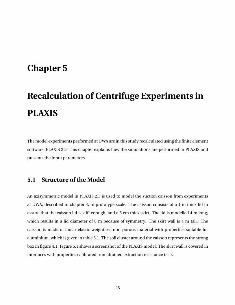
An axisymmetric model in PLAXIS 2D is used to model the suction caisson from experiments
at UWA, described in chapter 4, in prototype scale. The caisson consists of a 1 m thick lid to
assure that the caisson lid is stiff enough, and a 5 cm thick skirt. The lid is modelled 4 m long,
which results in a lid diameter of 8 m because of symmetry. The skirt wall is 4 m tall. The
caisson is made of linear elastic weightless non-porous material with properties suitable for
aluminium, which is given in table 5.1. The soil cluster around the caisson represents the strong
box in figure 4.1. Figure 5.1 shows a screenshot of the PLAXIS model. The skirt wall is covered in
interfaces with properties calibrated from drained extraction resistance tests.
25
26 CHAPTER 5. RECALCULATION OF CENTRIFUGE EXPERIMENTS IN PLAXIS
Table 5.1: Material parameters for caisson made of aluminium.
E [kN /m2] 70×106
ν [−] 0.34G [kN /m2] 26.12×10⁶
Eoed [kN /m2] 107.7×10⁶
Figure 5.1: A screenshot shows the caisson of the PLAXIS model used in the PLAXIS simulations.
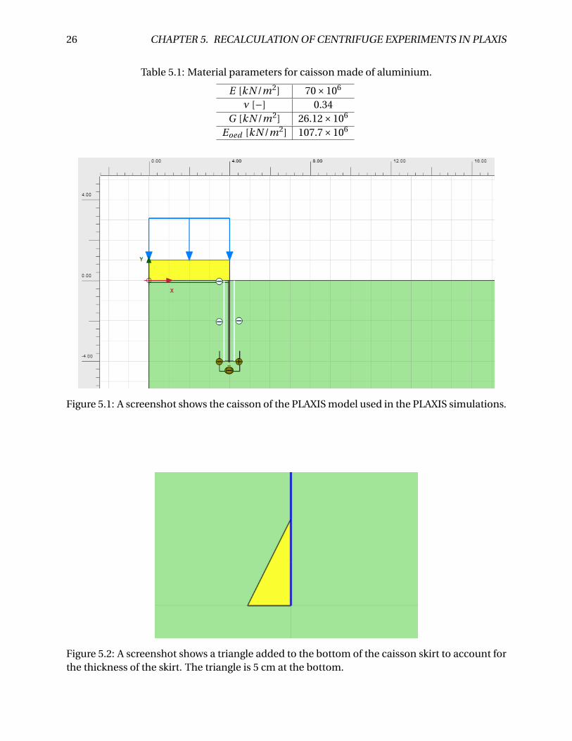
Figure 5.2: A screenshot shows a triangle added to the bottom of the caisson skirt to account forthe thickness of the skirt. The triangle is 5 cm at the bottom.
5.1. STRUCTURE OF THE MODEL 27
A simpler model where the caisson lid and skirt are made of stiff beam elements is also con-
sidered. This model is for instance used to calibrate drained extraction resistance. To include
thickness at the skirt tip, a soil triangle with stiffness similar to the aluminium skirt can be added
at the bottom of the skirt beam as shown in figure 5.2. An advantage using this model is reduc-
tion in required capacity needed to perform the calculation. This is due to the simpler con-
struction of caisson skirt and lid which require a less complicated mesh generation for the finite
element analysis. However, the capacity of most of today’s computers is large enough to han-
dle the extra iterations needed. In addition, the triangle can cause false moment because of its
non-symmetry. The model first introduced is therefore mainly used in the simulations.
5.1.1 Finite Element Mesh
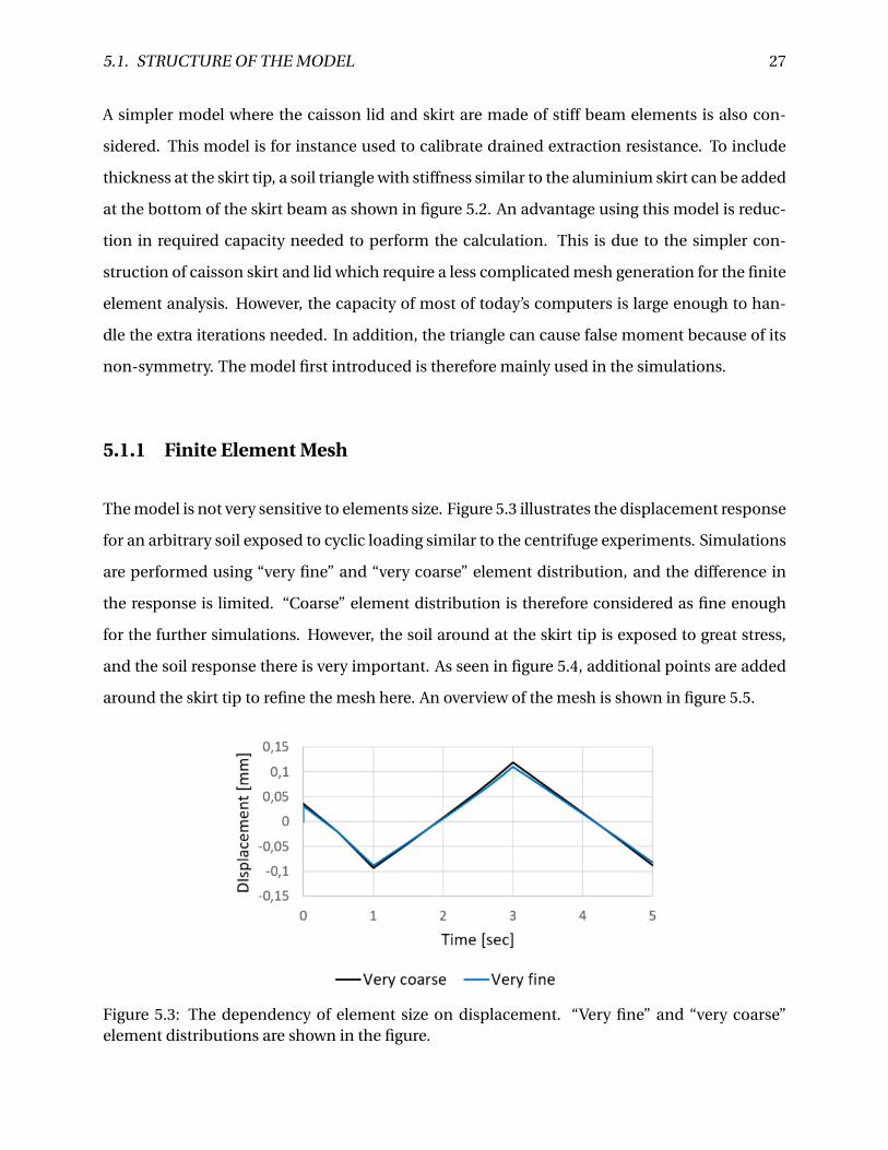
The model is not very sensitive to elements size. Figure 5.3 illustrates the displacement response
for an arbitrary soil exposed to cyclic loading similar to the centrifuge experiments. Simulations
are performed using “very fine” and “very coarse” element distribution, and the difference in
the response is limited. “Coarse” element distribution is therefore considered as fine enough
for the further simulations. However, the soil around at the skirt tip is exposed to great stress,
and the soil response there is very important. As seen in figure 5.4, additional points are added
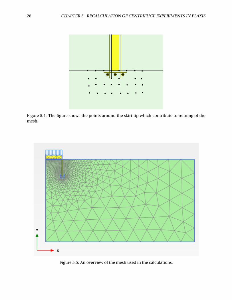
around the skirt tip to refine the mesh here. An overview of the mesh is shown in figure 5.5.
Figure 5.3: The dependency of element size on displacement. “Very fine” and “very coarse”element distributions are shown in the figure.
28 CHAPTER 5. RECALCULATION OF CENTRIFUGE EXPERIMENTS IN PLAXIS
Figure 5.4: The figure shows the points around the skirt tip which contribute to refining of themesh.
Figure 5.5: An overview of the mesh used in the calculations.
5.1. STRUCTURE OF THE MODEL 29
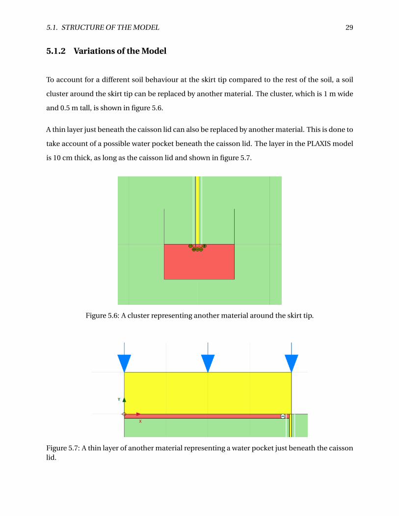
5.1.2 Variations of the Model
To account for a different soil behaviour at the skirt tip compared to the rest of the soil, a soil
cluster around the skirt tip can be replaced by another material. The cluster, which is 1 m wide
and 0.5 m tall, is shown in figure 5.6.
A thin layer just beneath the caisson lid can also be replaced by another material. This is done to
take account of a possible water pocket beneath the caisson lid. The layer in the PLAXIS model
is 10 cm thick, as long as the caisson lid and shown in figure 5.7.
Figure 5.6: A cluster representing another material around the skirt tip.
Figure 5.7: A thin layer of another material representing a water pocket just beneath the caissonlid.
30 CHAPTER 5. RECALCULATION OF CENTRIFUGE EXPERIMENTS IN PLAXIS
5.1.3 Calculation Types and Loading
The simulations in PLAXIS are conducted using different calculation types; plastic or consolida-
tion calculation. The plastic analyses are either fully drained or fully undrained. For all types of
calculations, the load is applied in several phases. Initially the mean stress is applied drained.
Subsequently a distributed load corresponding to the maximum applied compression stress is
applied, which marks the start of the cyclic loading. The soil is thereafter unloaded to its mean
stress, and further to its maximum load in tension. As the aim is to study the behaviour during
unloading and reloading, the soil must have experienced the current applied load earlier. To
satisfy this condition, the soil is once again loaded to its maximum compression load.
The consolidation calculations are supposed to represent the centrifuge experiments most pre-
cisely. The cyclic load is therefore applied with a frequency of 0.5 Hz which is similar to the
centrifuge experiments. This is accomplished by splitting one cyclic into four quarters and as-
sign one phase two each quarter. The time interval of each phase is set to 0.5 seconds. The same
response would have been possible to achieve by splitting the cycle in two. However, the use of
four phases per cycle makes it a lot easier to separate the response in tension and compression.
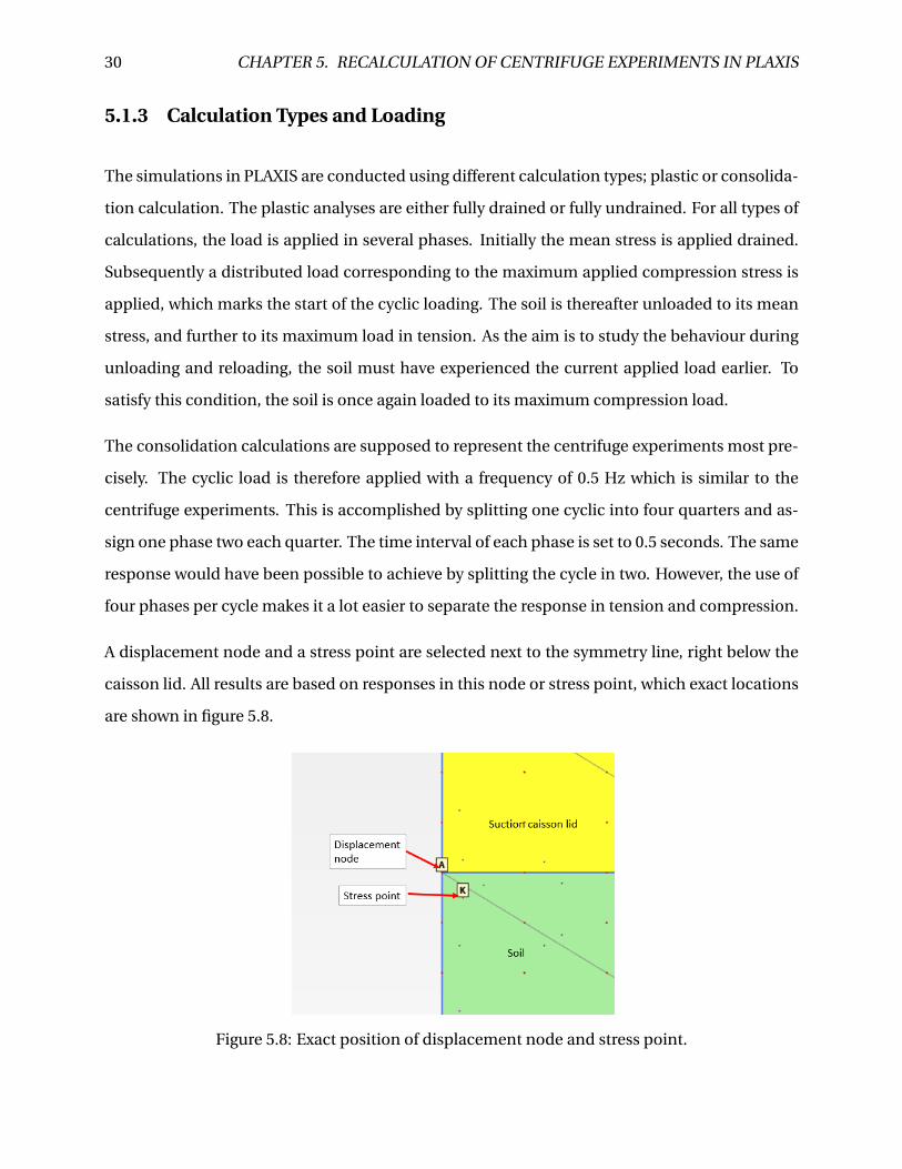
A displacement node and a stress point are selected next to the symmetry line, right below the
caisson lid. All results are based on responses in this node or stress point, which exact locations
are shown in figure 5.8.
Figure 5.8: Exact position of displacement node and stress point.
5.2. ADAPTION OF PARAMETERS 31
5.2 Adaption of Parameters
5.2.1 Stiffness Parameters for the Hardening Soil Model
The stiffness parameters E and m are determined by simulating basic soil lab tests in the Soil-
Test option in PLAXIS. In a report from Norwegian Geotechnical Institute (NGI) by Andersen
and Jostad (1999), a set of oedometer and triaxial tests performed on dense Baskarp sand are
presented. The results from these tests are reproduced as identically as possible by adjusting
stiffness parameters of the hardening soil model.
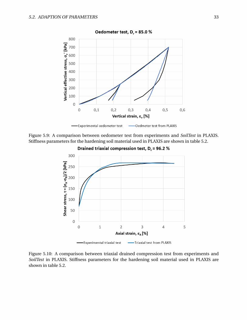
An oedometer test conducted on Baskarp sand with relative density Dr = 85 %, is here assumed
to have OC R = 1. A very good match between the results from the laboratory test and PLAXIS
simulation is achieved for the parameters listed in table 5.2. The estimation is illustrated in
figure 5.9. The result from the oedometer tests from Andersen and Jostad (1999) is here simplify
as the curve in reality has a different path for unloading and reloading. This would have been
visible at the curve from the oedometer test aroundσ′v = 200 kPa. However, the difference in the
unloading and reloading path is not captured by the hardening soil model.
The unloading stress path is dependent on the stress level of the soil prior to the unloading.
Consequently, the two unloading curves for the oedometer experiment in figure 5.9 have differ-
ent slopes. The unloading-reloading stiffness, Eur , is chosen to overestimate the stiffness of the
low-stress unloading path and underestimated the initial part of high-stress unloading path.
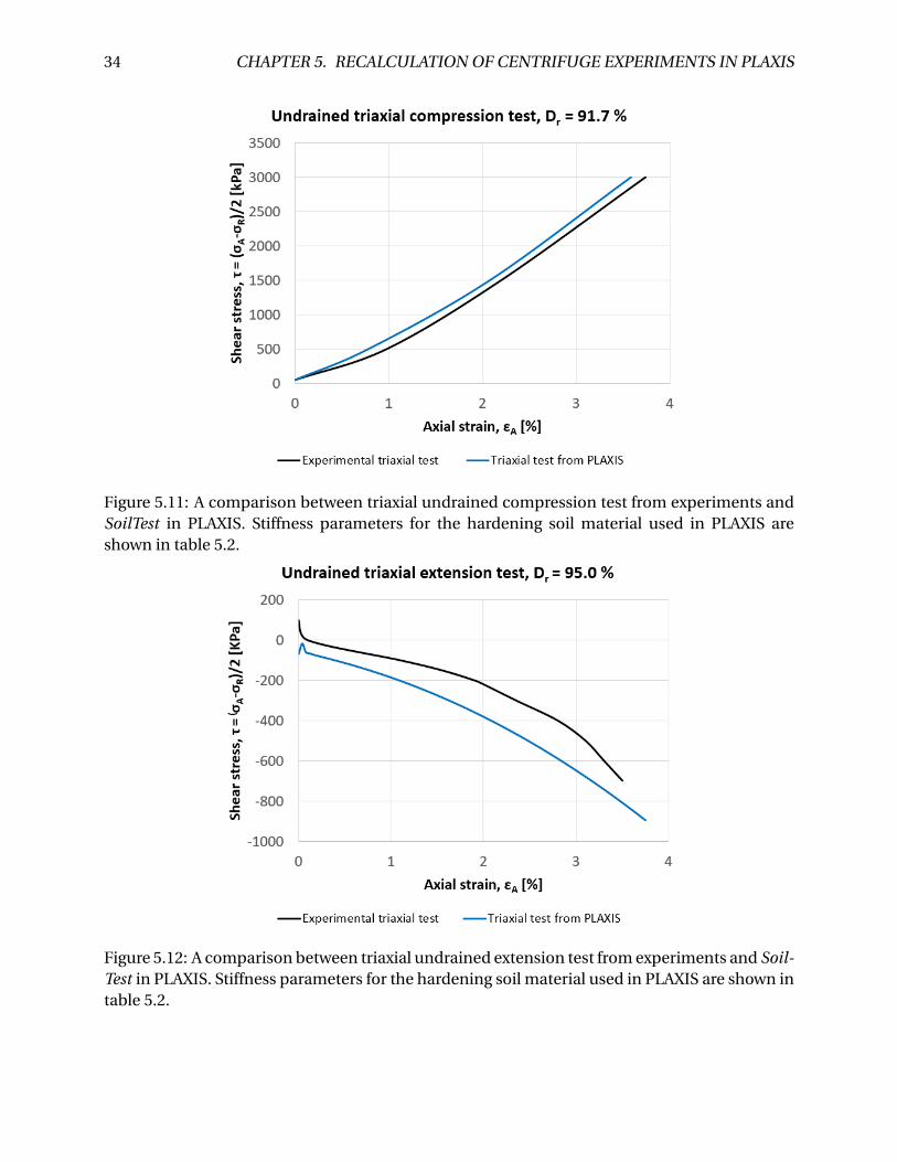
The two triaxial compression tests are anisotropically consolidated with vertical consolidation
stress σv = 250 kPa and horizontal consolidation stress σh = 112.5 kPa. The vertical stress in-
creases while the horizontal stress is kept constant during the tests. The results from the drained
and undrained tests are illustrated in figure 5.10 and 5.11, respectively. The stiffness parameters
are given in table 5.2. The reference stiffness for unloading and reloading, E r e fur , is chosen arbi-
trary as the soil specimens are not exposed to this type of loading.
An undrained triaxial extension test has been conducted by Andersen (1989). The anisotropic
consolidation is identical to the triaxial compression test, i.e. σv = 250kPa and σh = 112.5kPa.
The test is run by keeping the horizontal stress constant while reducing the vertical stress. The
result from the soil test is shown in figure 5.12.
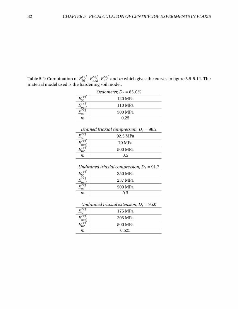
32 CHAPTER 5. RECALCULATION OF CENTRIFUGE EXPERIMENTS IN PLAXIS
Table 5.2: Combination of E r e f50 , E r e f
oed , E r e fur and m which gives the curves in figure 5.9-5.12. The
material model used is the hardening soil model.
Oedometer, Dr = 85,0%
E r e f50 120 MPa
E r e foed 110 MPa
E r e fur 500 MPam 0,25
Drained triaxial compression, Dr = 96.2
E r e f50 92.5 MPa
E r e foed 70 MPa
E r e fur 500 MPam 0.5
Undrained triaxial compression, Dr = 91.7
E r e f50 250 MPa
E r e foed 237 MPa
E r e fur 500 MPam 0.3
Undrained triaxial extension, Dr = 95.0
E r e f50 175 MPa
E r e foed 203 MPa
E r e fur 500 MPam 0.525
5.2. ADAPTION OF PARAMETERS 33
Figure 5.9: A comparison between oedometer test from experiments and SoilTest in PLAXIS.Stiffness parameters for the hardening soil material used in PLAXIS are shown in table 5.2.
Figure 5.10: A comparison between triaxial drained compression test from experiments andSoilTest in PLAXIS. Stiffness parameters for the hardening soil material used in PLAXIS areshown in table 5.2.
34 CHAPTER 5. RECALCULATION OF CENTRIFUGE EXPERIMENTS IN PLAXIS
Figure 5.11: A comparison between triaxial undrained compression test from experiments andSoilTest in PLAXIS. Stiffness parameters for the hardening soil material used in PLAXIS areshown in table 5.2.
Figure 5.12: A comparison between triaxial undrained extension test from experiments and Soil-Test in PLAXIS. Stiffness parameters for the hardening soil material used in PLAXIS are shown intable 5.2.
5.2. ADAPTION OF PARAMETERS 35
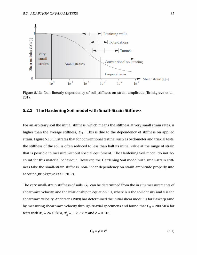
Figure 5.13: Non-linearly dependency of soil stiffness on strain amplitude (Brinkgreve et al.,2017).
5.2.2 The Hardening Soil model with Small-Strain Stiffness
For an arbitrary soil the initial stiffness, which means the stiffness at very small strain rates, is
higher than the average stiffness, E50. This is due to the dependency of stiffness on applied
strain. Figure 5.13 illustrates that for conventional testing, such as oedometer and triaxial tests,
the stiffness of the soil is often reduced to less than half its initial value at the range of strain
that is possible to measure without special equipment. The Hardening Soil model do not ac-
count for this material behaviour. However, the Hardening Soil model with small-strain stiff-
ness take the small-strain stiffness’ non-linear dependency on strain amplitude properly into
account (Brinkgreve et al., 2017).
The very small-strain stiffness of soils, G0, can be determined from the in situ measurements of
shear wave velocity, and the relationship in equation 5.1, where ρ is the soil density and ν is the
shear wave velocity. Andersen (1989) has determined the initial shear modulus for Baskarp sand
by measuring shear wave velocity through triaxial specimens and found that G0 = 200 MPa for
tests with σ′v = 249.9 kPa, σ′
h = 112,7 kPa and e = 0.518.
G0 = ρ×ν2 (5.1)
36 CHAPTER 5. RECALCULATION OF CENTRIFUGE EXPERIMENTS IN PLAXIS
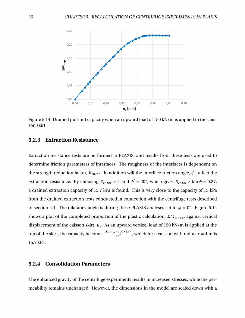
Figure 5.14: Drained pull-out capacity when an upward load of 150 kN/m is applied to the cais-son skirt.
5.2.3 Extraction Resistance
Extraction resistance tests are performed in PLAXIS, and results from these tests are used to
determine friction parameters of interfaces. The roughness of the interfaces is dependent on
the strength reduction factor, Ri nter . In addition will the interface friction angle, φ′, affect the
extraction resistance. By choosing Ri nter = 1 and φ′ = 20◦, which gives Ri nter × tanφ = 0.37,
a drained extraction capacity of 15.7 kPa is found. This is very close to the capacity of 15 kPa
from the drained extraction tests conducted in connection with the centrifuge tests described
in section 4.4. The dilatancy angle is during these PLAXIS analyses set to ψ = 0◦. Figure 5.14
shows a plot of the completed proportion of the plastic calculation, ΣMst ag e , against vertical
displacement of the caisson skirt, uy . As an upward vertical load of 150 kN/m is applied at the
top of the skirt, the capacity becomesMst ag e×150×2πr
πr 2 , which for a caisson with radius r = 4 m is
15.7 kPa.
5.2.4 Consolidation Parameters
The enhanced gravity of the centrifuge experiments results in increased stresses, while the per-
meability remains unchanged. However, the dimensions in the model are scaled down with a
5.2. ADAPTION OF PARAMETERS 37
factor identical to the enhancement of the gravitational acceleration. This means that the time
for consolidation to occur is different in the model and prototype. For both cases equation 5.2
from Terzaghi (1951) explains the relationship between time, soil volume and ability for fluid to
run through the soil pores.
t = Tv × h2
Cv(5.2)
h is the drainage path, Tv is the time factor and t is the time of consolidation. The coefficient
of consolidation, Cv , is identical for the model and prototype when the same soil is used. Tv is
dependent on normalised geometry and rate of drainage, and is consequently the same in the
model and prototype. Hence, the drainage path, h, is the only factor to change in addition to
the time.
The consolidation time for prototype and model is given in equation 5.3 and 5.4, respectively.
tpr otot y pe = Tv,pr otot y pe ×h2
pr otot y pe
Cv,pr otot y pe(5.3)
tmodel = Tv,model ×h2
model
Cv,model(5.4)
As the aim is to achieve the same degree of consolidation, Tv , equation 5.3 and 5.4 are used to
find the relationship between the time in prototype and model given in equation 5.5.
tmodel
tpr otot y pe=
(hmodel
hpr otot y pe
)2
= 1
N 2(5.5)
Considering the suction caisson under investigation, N = 100, which means that the whole
model test must be performed 1002 = 10000 times faster than the prototype. This is in prac-
tice very hard to accomplish. A more viscous fluid is therefore added to the soil sample. For
the samples with 100 cSt and 660 cSt pore fluid viscocity, the time to conduct the model tests
is extended 100 and 660 times, respectively. For modeling purpose, the remaining time differ-
38 CHAPTER 5. RECALCULATION OF CENTRIFUGE EXPERIMENTS IN PLAXIS
ence is accounted for by making the pore fluid dissipate faster as the permeability in the sim-
ulations is increased. The input value for permeability in PLAXIS has therefore changed from
k = 8.04×10⁻⁵m/s in the model experiments to k = 8.04×10⁻³ for test with 100 cSt pore fluid
viscosity and k = 0.53×10⁻³ for tests with 660 cSt pore fluid viscosity.
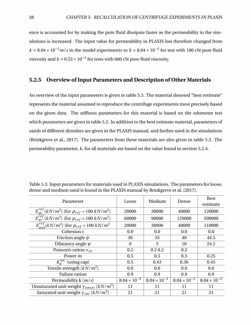
5.2.5 Overview of Input Parameters and Description of Other Materials
An overview of the input parameters is given in table 5.3. The material denoted “best estimate”
represents the material assumed to reproduce the centrifuge experiments most precisely based
on the given data. The stiffness parameters for this material is based on the odometer test
which parameters are given in table 5.2. In addition to the best estimate material, parameters of
sands of different densities are given in the PLAXIS manual, and further used in the simulations
(Brinkgreve et al., 2017). The parameters from these materials are also given in table 5.3. The
permeability parameter, k, for all materials are based on the value found in section 5.2.4.
Table 5.3: Input parameters for materials used in PLAXIS simulations. The parameters for loose,dense and medium sand is found in the PLAXIS manual by Brinkgreve et al. (2017).
Parameter Loose Medium DenseBest
estimate
E r e f50 [kN /m2] (for pr e f = 100 kN /m2) 20000 30000 40000 120000
E r e fur [kN /m2] (for pr e f = 100 kN /m2) 60000 90000 120000 500000
E r e foed [kN /m2] (for pr e f = 100 kN /m2 20000 30000 40000 110000
Cohesion c 0.0 0.0 0.0 0.0Friction angle φ 30 35 40 44.5
Dilatancy angle ψ 0 5 10 24.2Poisson’s ration νur 0.2 0.2 0.2 0.2
Power m 0.5 0.5 0.5 0.25K NC
0 (using cap) 0.5 0.43 0.36 0.45Tensile strength [kN /m2] 0.0 0.0 0.0 0.0
Failure ration 0.9 0.9 0.9 0.9Permeability k [m/s] 8.04×10⁻³ 8.04×10⁻³ 8.04×10⁻³ 8.04×10⁻³
Unsaturated unit weight γunsat [kN /m3] 11 11 11 11Saturated unit weight γsat [kN /m3] 21 21 21 21
Chapter 6
Results
This chapter presents the results from the centrifuge experiments conducted at UWA and recal-
culation of the same experiments using PLAXIS. The results are further discussed in chapter 7.
6.1 Centrifuge Experiments
Chapter 4 describes the procedure and basic principles of the centrifuge experiments conducted
at UWA. The applied loads from a test with different pore fluid viscosity, 100 cSt and 660 cSt
(named test 4-2 and 6-1 in Bienen et al. (2018a)), and approximately similar cyclic loading is
presented in table 6.1 and figure 6.1. The tests consist of four different load packets with con-
stant load amplitude. The target mean stress is 8 kPa for all load packets, but the achieved value
is slightly varying for the different load packets. Compression is defined positive and tension is
negative. The results from these two experiments are further examined.
39
40 CHAPTER 6. RESULTS
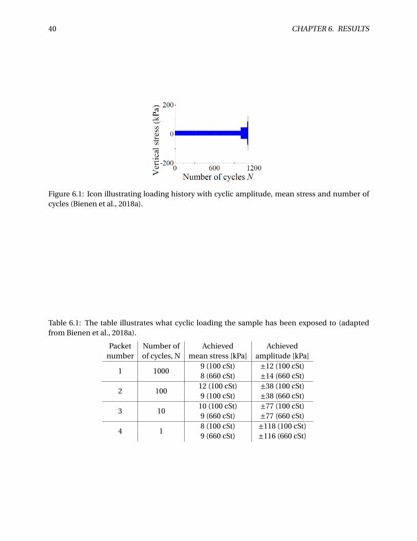
Figure 6.1: Icon illustrating loading history with cyclic amplitude, mean stress and number ofcycles (Bienen et al., 2018a).
Table 6.1: The table illustrates what cyclic loading the sample has been exposed to (adaptedfrom Bienen et al., 2018a).
Packet Number of Achieved Achievednumber of cycles, N mean stress [kPa] amplitude [kPa]
1 10009 (100 cSt) ±12 (100 cSt)8 (660 cSt) ±14 (660 cSt)
2 10012 (100 cSt) ±38 (100 cSt)9 (100 cSt) ±38 (660 cSt)
3 1010 (100 cSt) ±77 (100 cSt)9 (660 cSt) ±77 (660 cSt)
4 18 (100 cSt) ±118 (100 cSt)9 (660 cSt) ±116 (660 cSt)
6.1. CENTRIFUGE EXPERIMENTS 41
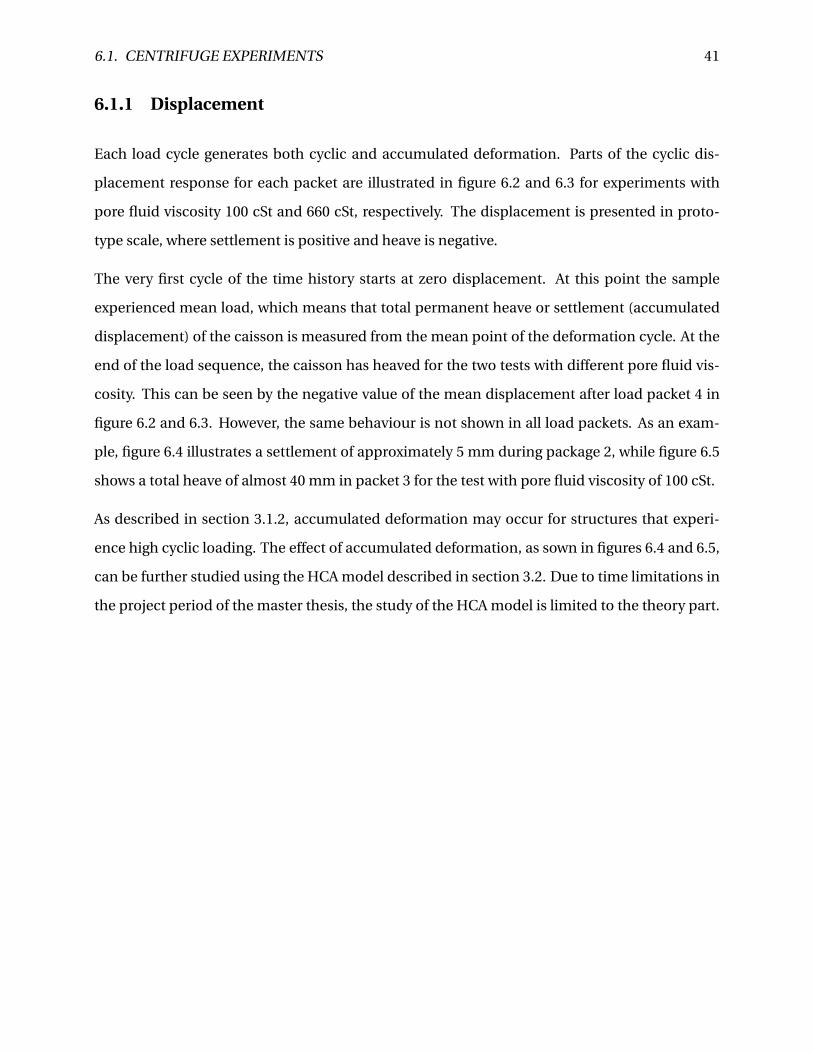
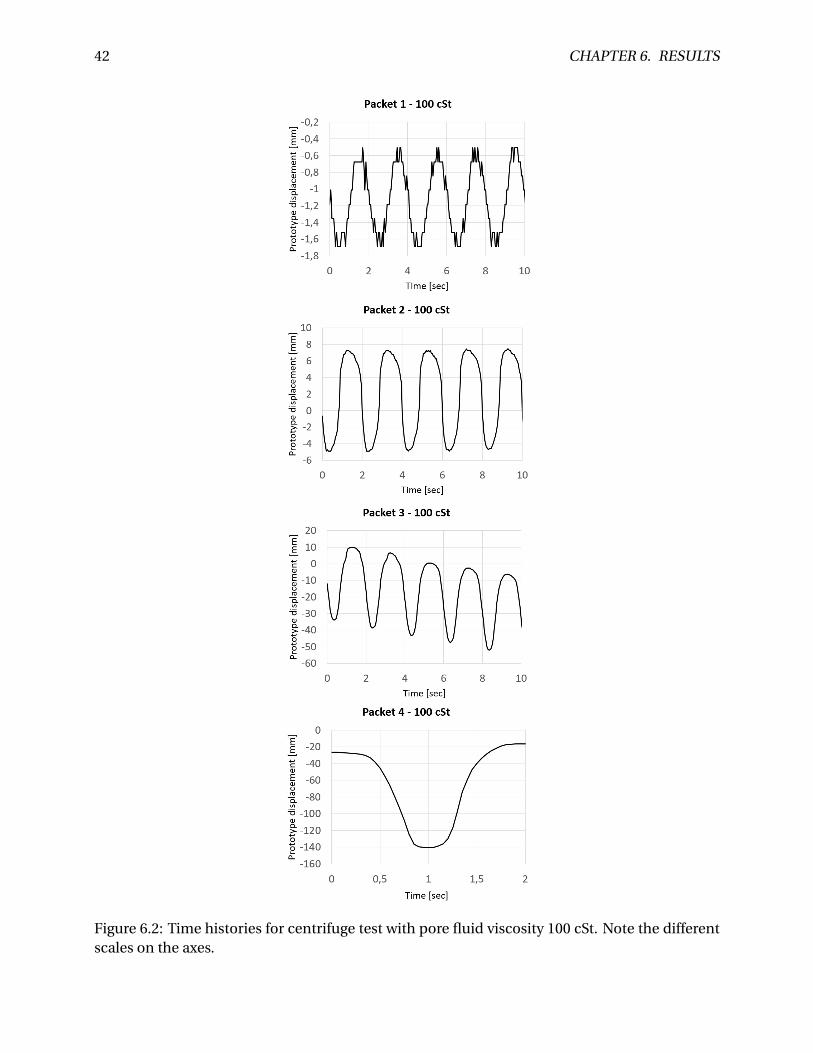
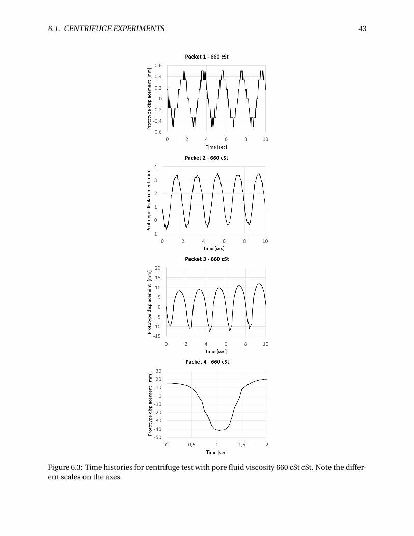
6.1.1 Displacement
Each load cycle generates both cyclic and accumulated deformation. Parts of the cyclic dis-
placement response for each packet are illustrated in figure 6.2 and 6.3 for experiments with
pore fluid viscosity 100 cSt and 660 cSt, respectively. The displacement is presented in proto-
type scale, where settlement is positive and heave is negative.
The very first cycle of the time history starts at zero displacement. At this point the sample
experienced mean load, which means that total permanent heave or settlement (accumulated
displacement) of the caisson is measured from the mean point of the deformation cycle. At the
end of the load sequence, the caisson has heaved for the two tests with different pore fluid vis-
cosity. This can be seen by the negative value of the mean displacement after load packet 4 in
figure 6.2 and 6.3. However, the same behaviour is not shown in all load packets. As an exam-
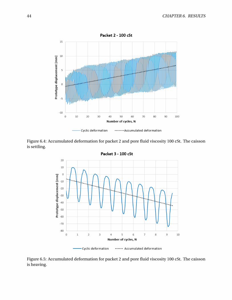
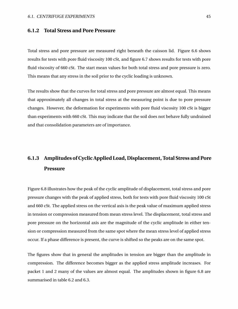
ple, figure 6.4 illustrates a settlement of approximately 5 mm during package 2, while figure 6.5
shows a total heave of almost 40 mm in packet 3 for the test with pore fluid viscosity of 100 cSt.
As described in section 3.1.2, accumulated deformation may occur for structures that experi-
ence high cyclic loading. The effect of accumulated deformation, as sown in figures 6.4 and 6.5,
can be further studied using the HCA model described in section 3.2. Due to time limitations in
the project period of the master thesis, the study of the HCA model is limited to the theory part.
42 CHAPTER 6. RESULTS
Figure 6.2: Time histories for centrifuge test with pore fluid viscosity 100 cSt. Note the differentscales on the axes.
6.1. CENTRIFUGE EXPERIMENTS 43
Figure 6.3: Time histories for centrifuge test with pore fluid viscosity 660 cSt cSt. Note the differ-ent scales on the axes.
44 CHAPTER 6. RESULTS
Figure 6.4: Accumulated deformation for packet 2 and pore fluid viscosity 100 cSt. The caissonis settling.
Figure 6.5: Accumulated deformation for packet 2 and pore fluid viscosity 100 cSt. The caissonis heaving.
6.1. CENTRIFUGE EXPERIMENTS 45
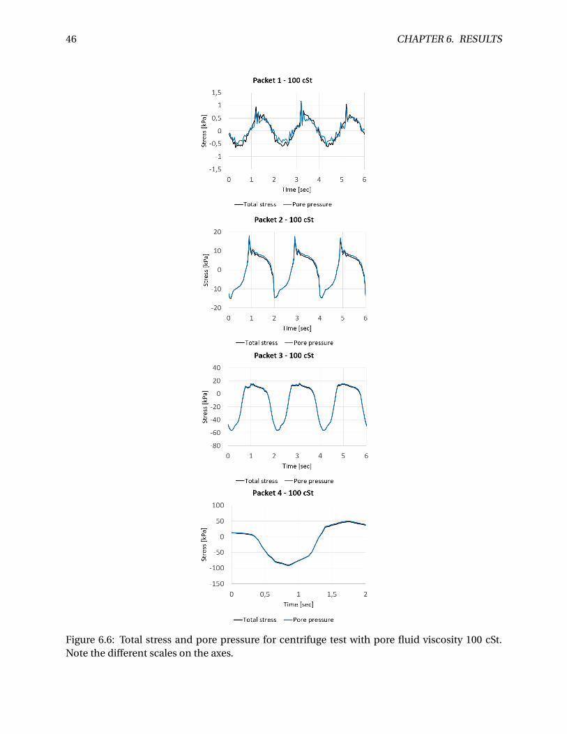
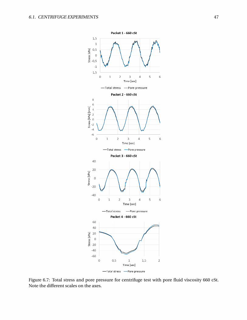
6.1.2 Total Stress and Pore Pressure
Total stress and pore pressure are measured right beneath the caisson lid. Figure 6.6 shows
results for tests with pore fluid viscosity 100 cSt, and figure 6.7 shows results for tests with pore
fluid viscosity of 660 cSt. The start mean values for both total stress and pore pressure is zero.
This means that any stress in the soil prior to the cyclic loading is unknown.
The results show that the curves for total stress and pore pressure are almost equal. This means
that approximately all changes in total stress at the measuring point is due to pore pressure
changes. However, the deformation for experiments with pore fluid viscosity 100 cSt is bigger
than experiments with 660 cSt. This may indicate that the soil does not behave fully undrained
and that consolidation parameters are of importance.
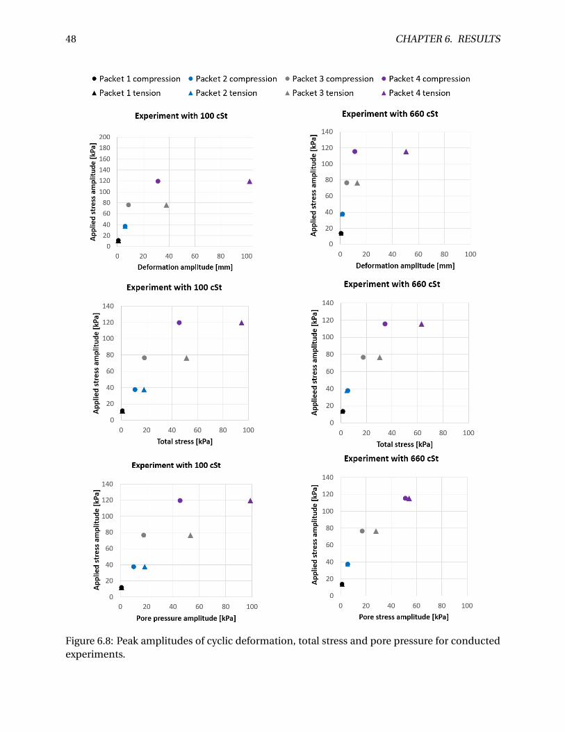
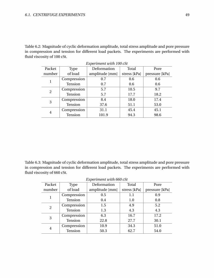
6.1.3 Amplitudes of Cyclic Applied Load, Displacement, Total Stress and Pore
Pressure
Figure 6.8 illustrates how the peak of the cyclic amplitude of displacement, total stress and pore
pressure changes with the peak of applied stress, both for tests with pore fluid viscosity 100 cSt
and 660 cSt. The applied stress on the vertical axis is the peak value of maximum applied stress
in tension or compression measured from mean stress level. The displacement, total stress and
pore pressure on the horizontal axis are the magnitude of the cyclic amplitude in either ten-
sion or compression measured from the same spot where the mean stress level of applied stress
occur. If a phase difference is present, the curve is shifted so the peaks are on the same spot.
The figures show that in general the amplitudes in tension are bigger than the amplitude in
compression. The difference becomes bigger as the applied stress amplitude increases. For
packet 1 and 2 many of the values are almost equal. The amplitudes shown in figure 6.8 are
summarised in table 6.2 and 6.3.
46 CHAPTER 6. RESULTS
Figure 6.6: Total stress and pore pressure for centrifuge test with pore fluid viscosity 100 cSt.Note the different scales on the axes.
6.1. CENTRIFUGE EXPERIMENTS 47
Figure 6.7: Total stress and pore pressure for centrifuge test with pore fluid viscosity 660 cSt.Note the different scales on the axes.
48 CHAPTER 6. RESULTS
Figure 6.8: Peak amplitudes of cyclic deformation, total stress and pore pressure for conductedexperiments.
6.1. CENTRIFUGE EXPERIMENTS 49
Table 6.2: Magnitude of cyclic deformation amplitude, total stress amplitude and pore pressurein compression and tension for different load packets. The experiments are performed withfluid viscosity of 100 cSt.
Experiment with 100 cStPacket Type Deformation Total Pore
number of load amplitude [mm] stress [kPa] pressure [kPa]
1Compression 0.7 0.6 0.6
Tension 0.7 0.6 0.6
2Compression 5.7 10.5 9.7
Tension 5.7 17.7 18.2
3Compression 8.4 18.0 17.4
Tension 37.6 51.1 53.0
4Compression 31.1 45.4 45.1
Tension 101.9 94.3 98.6
Table 6.3: Magnitude of cyclic deformation amplitude, total stress amplitude and pore pressurein compression and tension for different load packets. The experiments are performed withfluid viscosity of 660 cSt.
Experiment with 660 cStPacket Type Deformation Total Pore
number of load amplitude [mm] stress [kPa] pressure [kPa]
1Compression 0.5 1.1 0.9
Tension 0.4 1.0 0.8
2Compression 1.5 4.9 5.2
Tension 1.3 4.3 4.3
3Compression 6.3 16.7 17.2
Tension 22.8 27.7 30.1
4Compression 10.9 34.3 51.0
Tension 50.3 62.7 54.0
50 CHAPTER 6. RESULTS
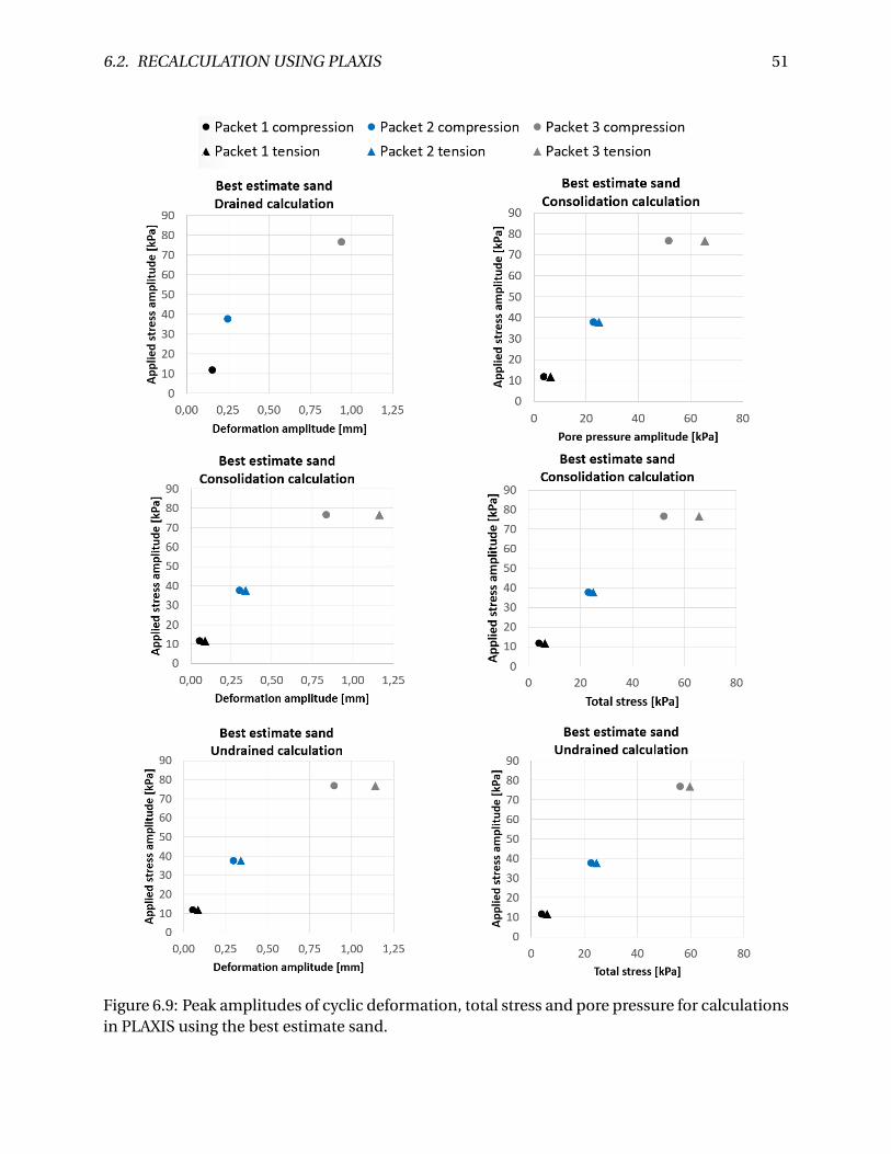
6.2 Recalculation Using PLAXIS
The centrifuge experiment with cyclic loading as in figure 6.1 is recalculated using PLAXIS. Dif-
ferent calculation types are used to understand how the model works. The simulations are pre-
formed as plastic analyses, either fully drained or fully undrained, or as consolidation analyses
where the cyclic load is applied with a frequency of 0.5 Hz, similar to the centrifuge experiments.
The material adapted to the oedometer test, which stiffness parameters are shown in table 5.2,
is considered as a best estimate material. The materials with different densities, presented in
table 5.3, are also used in the simulations.
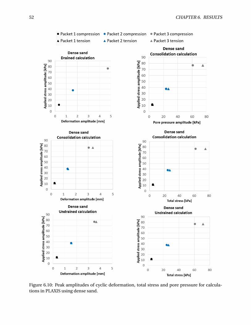
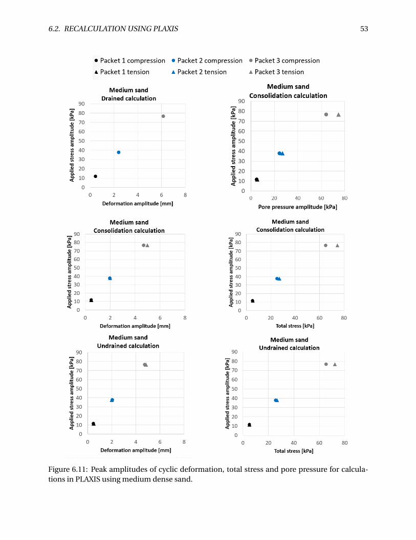
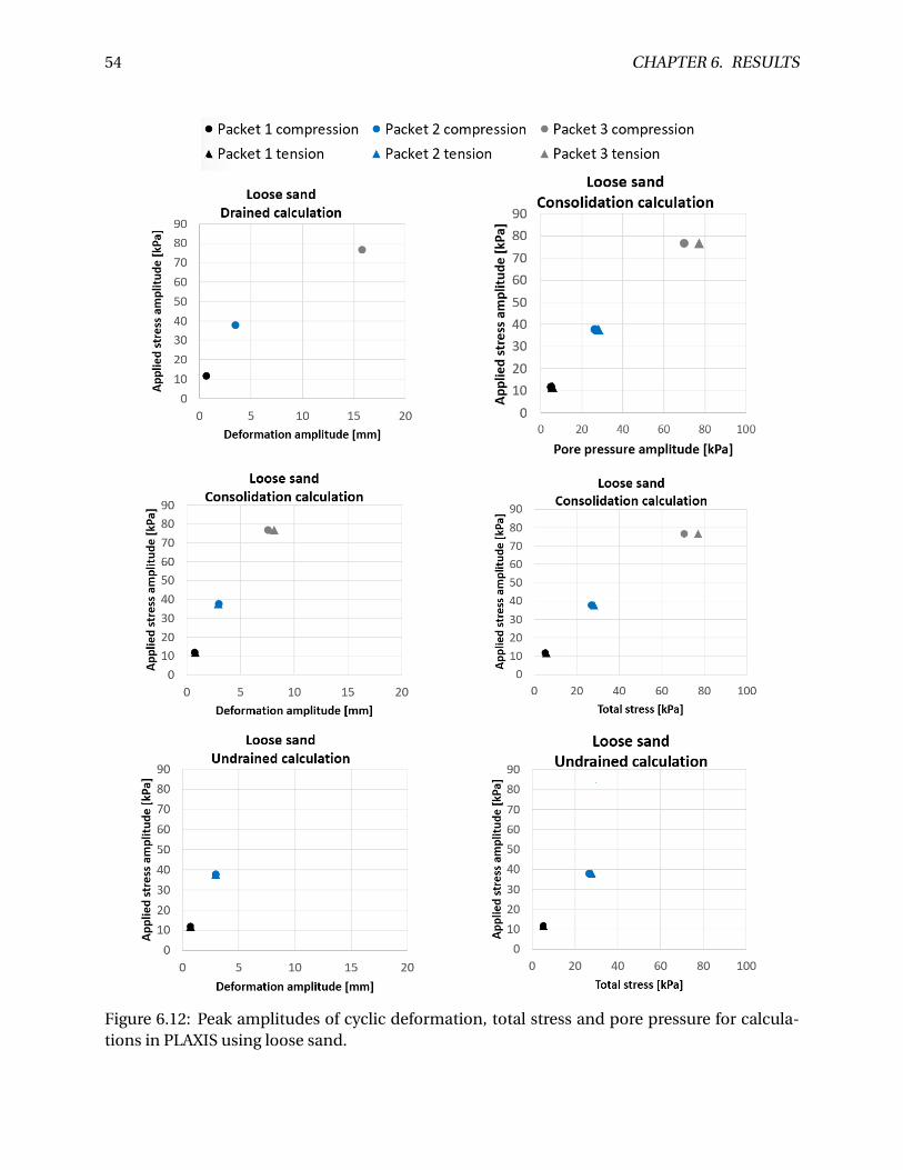
Figures for cyclic peak amplitudes for displacements, total stress and pore pressures in PLAXIS
simulations are presented. This corresponds to the peak amplitudes shown in figure 6.8 for
centrifuge tests. Figure 6.9 presents results from simulations using best estimate sand, figure
6.10 presents results from dense sand, figure 6.11 presents results from medium dense sand and
6.12 presents results from loose sand. Table 6.4 summarises the values in figure 6.9 to 6.12.
The results show the same pattern as can be seen for the centrifuge experiments, with bigger
amplitudes in tension than in compression, and a difference between compression and tension
which becomes larger with the applied stress amplitude.
As the model in PLAXIS goes to failure when loaded to packet 4, no results of PLAXIS simulations
from this packet is presented. This also applies to the fully undrained calculations in packet 3
for loose sand.
A comparison of the results from centrifuge tests and PLAXIS simulations is presented for peak
amplitude displacements in figure 6.13, total stress in figure 6.14 and pore pressure in figure
6.15. In general, the deformation is underestimated and the total stress and pore pressure are
overestimated in the PLAXIS simulations.
6.2. RECALCULATION USING PLAXIS 51
Figure 6.9: Peak amplitudes of cyclic deformation, total stress and pore pressure for calculationsin PLAXIS using the best estimate sand.
52 CHAPTER 6. RESULTS
Figure 6.10: Peak amplitudes of cyclic deformation, total stress and pore pressure for calcula-tions in PLAXIS using dense sand.
6.2. RECALCULATION USING PLAXIS 53
Figure 6.11: Peak amplitudes of cyclic deformation, total stress and pore pressure for calcula-tions in PLAXIS using medium dense sand.
54 CHAPTER 6. RESULTS
Figure 6.12: Peak amplitudes of cyclic deformation, total stress and pore pressure for calcula-tions in PLAXIS using loose sand.
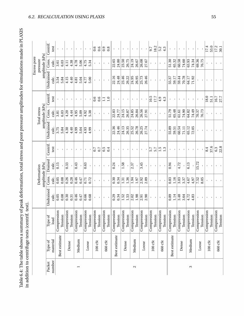
6.2. RECALCULATION USING PLAXIS 55Ta
ble
6.4:
Th
eta
ble
show
sa
sum
mar
yo
fpea
kd
efo
rmat
ion
,to
tals
tres
san
dp
ore
pre
ssu
ream
pli
tud
esfo
rsim
ula
tio
ns
mad
ein
PL
AX
ISin
add
itio
nto
cen
trif
uge
test
s(c
entr
if.t
est)
.
Exc
ess
po
reD
efo
rmat
ion
Tota
lstr
ess
pre
ssu
ream
pli
tud
e[k
Pa]
amp
litu
de
[kPa
]am
pli
tud
e[k
Pa]
Pack
etTy
pe
of
Typ
eo
fU
nd
rain
edC
on
s.D
rain
edC
entr
if.
Un
dra
ined
Co
ns.
Cen
trif
.U
nd
rain
edC
on
s.C
entr
if.
nu
mb
erm
ater
ial
load
calc
.ca
lc.
calc
.te
stca
lc.
calc
.te
stca
lc.
calc
.te
st
1
Bes
test
imat
eC
om
pre
ssio
n0.
050.
050.
15-
3.75
3.81
-3.
543.
61-
Ten
sio
n0.
080.
08-
-5.
846.
03-
5.84
6.03
-
Den
seC
om
pre
ssio
n0.
300.
260.
33-
4.30
4.20
-4.
154.
11-
Ten
sio
n0.
310.
28-
-4.
404.
44-
4.40
4.38
-
Med
ium
Co
mp
ress
ion
0.46
0.46
0.43
-4.
994.
95-
4.81
4.78
-Te
nsi
on
0.47
0.47
--
5.04
5.09
-5.
045.
06-
Loo
seC
om
pre
ssio
n0.
660.
710.
63-
4.93
4.92
-4.
774.
75-
Ten
sio
n0.
680.
72-
-4.
995.
38-
5.00
5.34
-
100
cSt
Co
mp
ress
ion
--
-0.
7-
-0.
6-
-0.
6Te
nsi
on
--
-0.
7-
-0.
6-
-0.
6
660
cSt
Co
mp
ress
ion
--
-0.
5-
-1.
1-
-0.
9Te
nsi
on
--
-0.
4-
-1.
0-
-0.
8
2
Bes
test
imat
eC
om
pre
ssio
n0.
290.
300.
24-
22.3
622
.83
-22
.16
22.6
5-
Ten
sio
n0.
340.
34-
-24
.46
24.7
7-
24.4
824
.80
-
Den
seC
om
pre
ssio
n1.
521.
311.
58-
24.1
324
.15
-23
.46
23.5
0-
Ten
sio
n1.
531.
36-
-26
.35
26.8
7-
26.2
226
.75
-
Med
ium
Co
mp
ress
ion
2.02
1.94
2.37
-25
.52
24.8
5-
24.9
524
.19
-Te
nsi
on
1.98
1.97
--
26.7
826
.84
-26
.95
26.6
7-
Loo
seC
om
pre
ssio
n2.
912.
923.
45-
26.2
526
.56
-25
.73
26.0
8-
Ten
sio
n2.
902.
89-
-27
.74
27.9
1-
26.4
627
.67
-
100
cSt
Co
mp
ress
ion
--
-5.
7-
-10
.5-
-9.
7Te
nsi
on
--
-5.
7-
-17
.7-
-18
.2
660
cSt
Co
mp
ress
ion
--
-1.
5-
-4.
9-
-5.
2Te
nsi
on
--
-1.
3-
-4.
3-
-4.
3
3
Bes
test
imat
eC
om
pre
ssio
n0.
890.
830.
94-
55.8
951
.79
-55
.37
51.3
0-
Ten
sio
n1.
141.
16-
-59
.51
65.4
8-
59.1
765
.32
-
Den
seC
om
pre
ssio
n3.
483.
034.
72-
60.5
461
.61
-59
.44
60.5
8-
Ten
sio
n3.
643.
37-
-71
.11
74.9
0-
70.7
874
.60
-
Med
ium
Co
mp
ress
ion
4.72
4.67
6.13
-65
.12
64.8
2-
64.1
763
.93
-Te
nsi
on
4.83
4,97
--
72.0
574
.49
-71
.92
74.3
4-
Loo
seC
om
pre
ssio
n-
7.52
15.7
2-
-70
.37
--
69.3
6-
Ten
sio
n-
8.05
--
-76
.73
--
76.7
5-
100
cSt
Co
mp
ress
ion
--
-8.
4-
-18
.0-
-17
.4Te
nsi
on
--
-37
.6-
-51
.1-
-53
.0
660
cSt
Co
mp
ress
ion
--
-6.
3-
-16
.7-
-17
.2Te
nsi
on
--
-22
.8-
-27
.7-
-30
.1
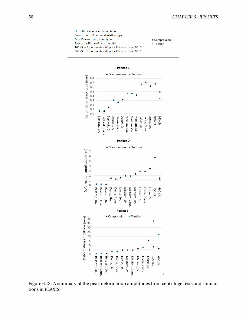
56 CHAPTER 6. RESULTS
’
Figure 6.13: A summary of the peak deformation amplitudes from centrifuge tests and simula-tions in PLAXIS.
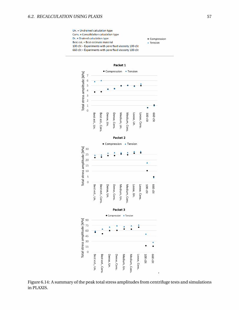
6.2. RECALCULATION USING PLAXIS 57
’
Figure 6.14: A summary of the peak total stress amplitudes from centrifuge tests and simulationsin PLAXIS.
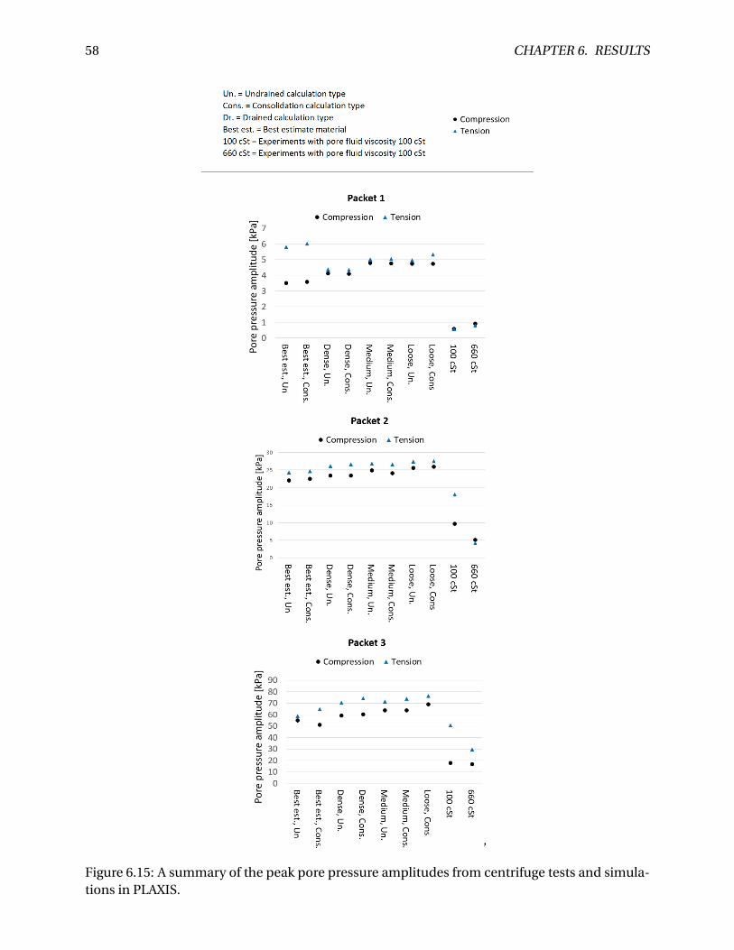
58 CHAPTER 6. RESULTS
’
Figure 6.15: A summary of the peak pore pressure amplitudes from centrifuge tests and simula-tions in PLAXIS.
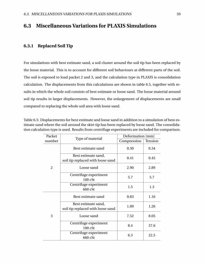
6.3. MISCELLANEOUS VARIATIONS FOR PLAXIS SIMULATIONS 59
6.3 Miscellaneous Variations for PLAXIS Simulations
6.3.1 Replaced Soil Tip
For simulations with best estimate sand, a soil cluster around the soil tip has been replaced by
the loose material. This is to account for different soil behaviours at different parts of the soil.
The soil is exposed to load packet 2 and 3, and the calculation type in PLAXIS is consolidation
calculation. The displacements from this calculations are shown in table 6.5, together with re-
sults in which the whole soil consists of best estimate or loose sand. The loose material around
soil tip results in larger displacements. However, the enlargement of displacements are small
compared to replacing the whole soil area with loose sand.
Table 6.5: Displacements for best estimate and loose sand in addition to a simulation of best es-timate sand where the soil around the skirt tip has been replaced by loose sand. The consolida-tion calculation type is used. Results from centrifuge experiments are included for comparison.
PacketType of material
Deformation [mm]number Compression Tension
2
Best estimate sand 0.30 0.34
Best estimate sand,0.41 0.45
soil tip replaced with loose sand
Loose sand 2.90 2.89
Centrifuge experiment5.7 5.7
100 cStCentrifuge experiment
1.5 1.3660 cSt
3
Best estimate sand 0.83 1.16
Best estimate sand,1.09 1.26
soil tip replaced with loose sand
Loose sand 7.52 8.05
Centrifuge experiment8.4 37.6
100 cStCentrifuge experiment
6.3 22.5660 cSt
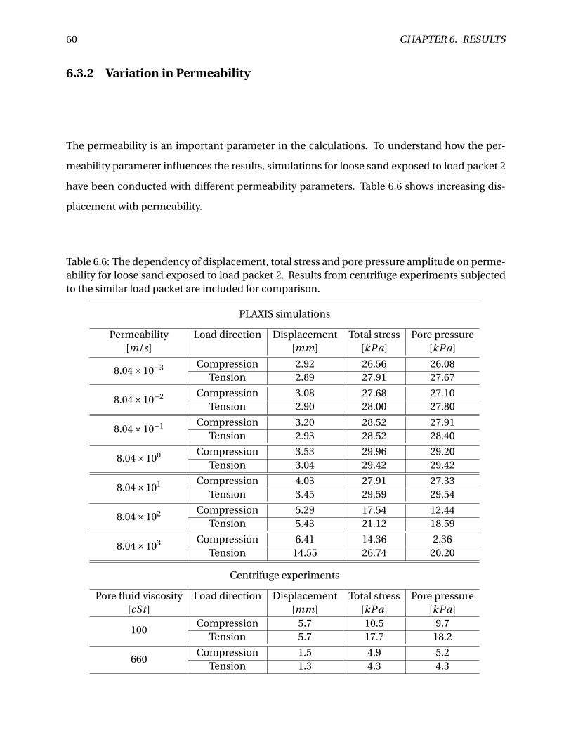
60 CHAPTER 6. RESULTS
6.3.2 Variation in Permeability
The permeability is an important parameter in the calculations. To understand how the per-
meability parameter influences the results, simulations for loose sand exposed to load packet 2
have been conducted with different permeability parameters. Table 6.6 shows increasing dis-
placement with permeability.
Table 6.6: The dependency of displacement, total stress and pore pressure amplitude on perme-ability for loose sand exposed to load packet 2. Results from centrifuge experiments subjectedto the similar load packet are included for comparison.
PLAXIS simulations
Permeability Load direction Displacement Total stress Pore pressure[m/s] [mm] [kPa] [kPa]
8.04×10⁻³ Compression 2.92 26.56 26.08Tension 2.89 27.91 27.67
8.04×10⁻² Compression 3.08 27.68 27.10Tension 2.90 28.00 27.80
8.04×10⁻¹ Compression 3.20 28.52 27.91Tension 2.93 28.52 28.40
8.04×100 Compression 3.53 29.96 29.20Tension 3.04 29.42 29.42
8.04×101 Compression 4.03 27.91 27.33Tension 3.45 29.59 29.54
8.04×10² Compression 5.29 17.54 12.44Tension 5.43 21.12 18.59
8.04×10³ Compression 6.41 14.36 2.36Tension 14.55 26.74 20.20
Centrifuge experiments
Pore fluid viscosity Load direction Displacement Total stress Pore pressure[cSt ] [mm] [kPa] [kPa]
100Compression 5.7 10.5 9.7
Tension 5.7 17.7 18.2
660Compression 1.5 4.9 5.2
Tension 1.3 4.3 4.3
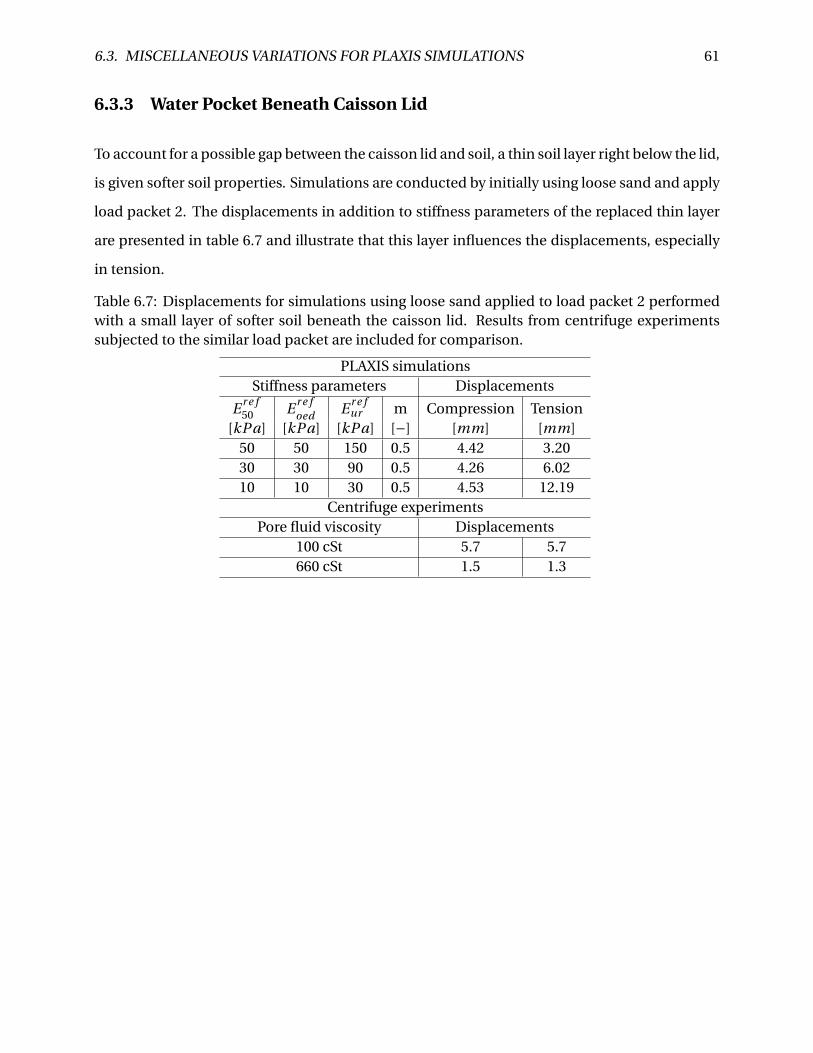
6.3. MISCELLANEOUS VARIATIONS FOR PLAXIS SIMULATIONS 61
6.3.3 Water Pocket Beneath Caisson Lid
To account for a possible gap between the caisson lid and soil, a thin soil layer right below the lid,
is given softer soil properties. Simulations are conducted by initially using loose sand and apply
load packet 2. The displacements in addition to stiffness parameters of the replaced thin layer
are presented in table 6.7 and illustrate that this layer influences the displacements, especially
in tension.
Table 6.7: Displacements for simulations using loose sand applied to load packet 2 performedwith a small layer of softer soil beneath the caisson lid. Results from centrifuge experimentssubjected to the similar load packet are included for comparison.
PLAXIS simulationsStiffness parameters Displacements
E r e f50 E r e f
oed E r e fur m Compression Tension
[kPa] [kPa] [kPa] [−] [mm] [mm]50 50 150 0.5 4.42 3.2030 30 90 0.5 4.26 6.0210 10 30 0.5 4.53 12.19
Centrifuge experimentsPore fluid viscosity Displacements
100 cSt 5.7 5.7660 cSt 1.5 1.3

Chapter 7
Discussion
In the following chapter the results from chapter 6 will be discussed. Firstly, cyclic peak am-
plitudes, including results from centrifuge experiments and simulations will be considered, fol-
lowed by examination of the type of behaviour and choice of material. Finally, the reasons for
difference in response in centrifuge experiments and PLAXIS simulations are discussed, hereun-
der loosening of soil due to installation, consolidation and redistribution of forces, gap between
caisson lid and soil in addition to air bubbles in the pore fluid.
7.1 Discussion on Cyclic Peak Amplitudes
This section presents a discussion on the cyclic peak amplitudes from centrifuge experiments
and PLAXIS simulations.
7.1.1 Centrifuge Experiments
The cyclic peak amplitudes from centrifuge experiments shown in figure 6.8 reveal that the de-
formation amplitudes increase non-linearly with applied stress amplitude. To emphasise the
non-linear behaviour, examples of regression lines are added to the results in figure 7.1. As can
63
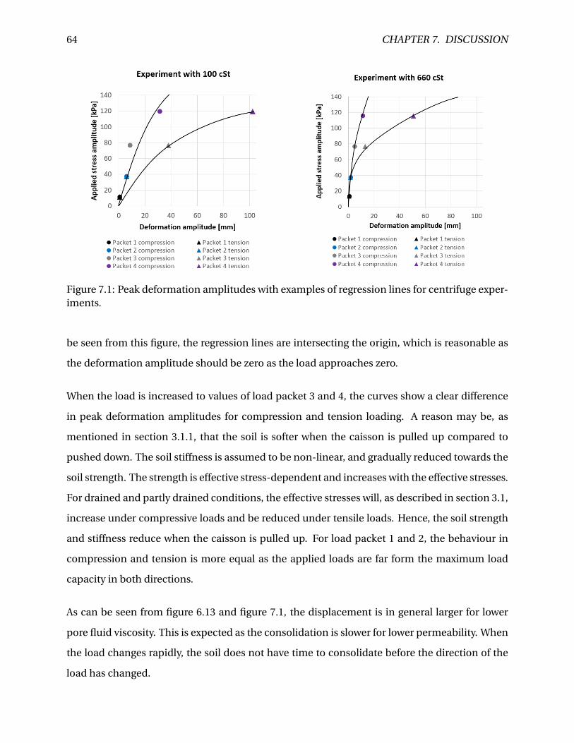
64 CHAPTER 7. DISCUSSION
Figure 7.1: Peak deformation amplitudes with examples of regression lines for centrifuge exper-iments.
be seen from this figure, the regression lines are intersecting the origin, which is reasonable as
the deformation amplitude should be zero as the load approaches zero.
When the load is increased to values of load packet 3 and 4, the curves show a clear difference
in peak deformation amplitudes for compression and tension loading. A reason may be, as
mentioned in section 3.1.1, that the soil is softer when the caisson is pulled up compared to
pushed down. The soil stiffness is assumed to be non-linear, and gradually reduced towards the
soil strength. The strength is effective stress-dependent and increases with the effective stresses.
For drained and partly drained conditions, the effective stresses will, as described in section 3.1,
increase under compressive loads and be reduced under tensile loads. Hence, the soil strength
and stiffness reduce when the caisson is pulled up. For load packet 1 and 2, the behaviour in
compression and tension is more equal as the applied loads are far form the maximum load
capacity in both directions.
As can be seen from figure 6.13 and figure 7.1, the displacement is in general larger for lower
pore fluid viscosity. This is expected as the consolidation is slower for lower permeability. When
the load changes rapidly, the soil does not have time to consolidate before the direction of the
load has changed.
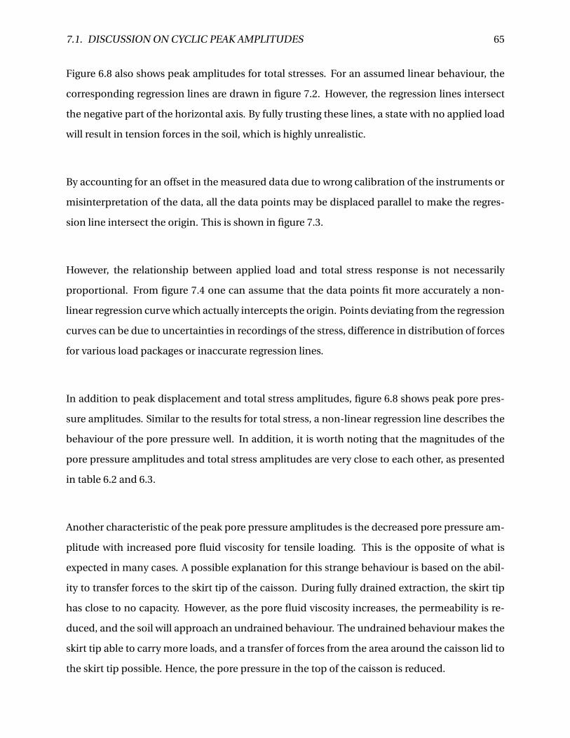
7.1. DISCUSSION ON CYCLIC PEAK AMPLITUDES 65
Figure 6.8 also shows peak amplitudes for total stresses. For an assumed linear behaviour, the
corresponding regression lines are drawn in figure 7.2. However, the regression lines intersect
the negative part of the horizontal axis. By fully trusting these lines, a state with no applied load
will result in tension forces in the soil, which is highly unrealistic.
By accounting for an offset in the measured data due to wrong calibration of the instruments or
misinterpretation of the data, all the data points may be displaced parallel to make the regres-
sion line intersect the origin. This is shown in figure 7.3.
However, the relationship between applied load and total stress response is not necessarily
proportional. From figure 7.4 one can assume that the data points fit more accurately a non-
linear regression curve which actually intercepts the origin. Points deviating from the regression
curves can be due to uncertainties in recordings of the stress, difference in distribution of forces
for various load packages or inaccurate regression lines.
In addition to peak displacement and total stress amplitudes, figure 6.8 shows peak pore pres-
sure amplitudes. Similar to the results for total stress, a non-linear regression line describes the
behaviour of the pore pressure well. In addition, it is worth noting that the magnitudes of the
pore pressure amplitudes and total stress amplitudes are very close to each other, as presented
in table 6.2 and 6.3.
Another characteristic of the peak pore pressure amplitudes is the decreased pore pressure am-
plitude with increased pore fluid viscosity for tensile loading. This is the opposite of what is
expected in many cases. A possible explanation for this strange behaviour is based on the abil-
ity to transfer forces to the skirt tip of the caisson. During fully drained extraction, the skirt tip
has close to no capacity. However, as the pore fluid viscosity increases, the permeability is re-
duced, and the soil will approach an undrained behaviour. The undrained behaviour makes the
skirt tip able to carry more loads, and a transfer of forces from the area around the caisson lid to
the skirt tip possible. Hence, the pore pressure in the top of the caisson is reduced.
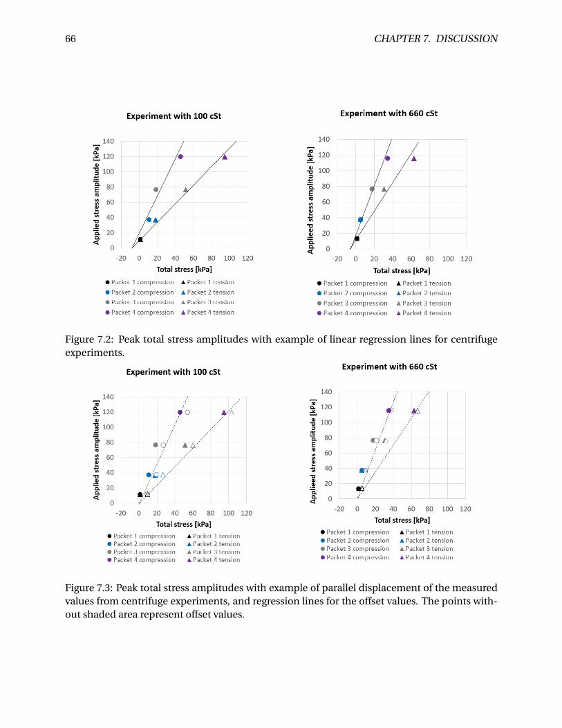
66 CHAPTER 7. DISCUSSION
Figure 7.2: Peak total stress amplitudes with example of linear regression lines for centrifugeexperiments.
Figure 7.3: Peak total stress amplitudes with example of parallel displacement of the measuredvalues from centrifuge experiments, and regression lines for the offset values. The points with-out shaded area represent offset values.
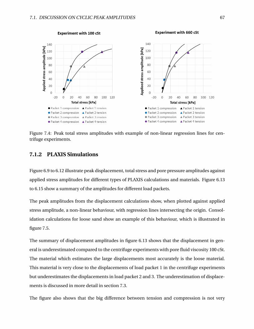
7.1. DISCUSSION ON CYCLIC PEAK AMPLITUDES 67
Figure 7.4: Peak total stress amplitudes with example of non-linear regression lines for cen-trifuge experiments.
7.1.2 PLAXIS Simulations
Figure 6.9 to 6.12 illustrate peak displacement, total stress and pore pressure amplitudes against
applied stress amplitudes for different types of PLAXIS calculations and materials. Figure 6.13
to 6.15 show a summary of the amplitudes for different load packets.
The peak amplitudes from the displacement calculations show, when plotted against applied
stress amplitude, a non-linear behaviour, with regression lines intersecting the origin. Consol-
idation calculations for loose sand show an example of this behaviour, which is illustrated in
figure 7.5.
The summary of displacement amplitudes in figure 6.13 shows that the displacement in gen-
eral is underestimated compared to the centrifuge experiments with pore fluid viscosity 100 cSt.
The material which estimates the large displacements most accurately is the loose material.
This material is very close to the displacements of load packet 1 in the centrifuge experiments
but underestimates the displacements in load packet 2 and 3. The underestimation of displace-
ments is discussed in more detail in section 7.3.
The figure also shows that the big difference between tension and compression is not very
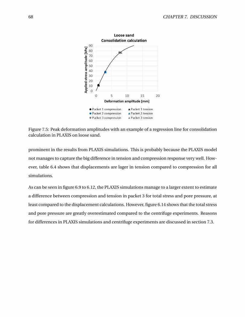
68 CHAPTER 7. DISCUSSION
Figure 7.5: Peak deformation amplitudes with an example of a regression line for consolidationcalculation in PLAXIS on loose sand.
prominent in the results from PLAXIS simulations. This is probably because the PLAXIS model
not manages to capture the big difference in tension and compression response very well. How-
ever, table 6.4 shows that displacements are lager in tension compared to compression for all
simulations.
As can be seen in figure 6.9 to 6.12, the PLAXIS simulations manage to a larger extent to estimate
a difference between compression and tension in packet 3 for total stress and pore pressure, at
least compared to the displacement calculations. However, figure 6.14 shows that the total stress
and pore pressure are greatly overestimated compared to the centrifuge experiments. Reasons
for differences in PLAXIS simulations and centrifuge experiments are discussed in section 7.3.
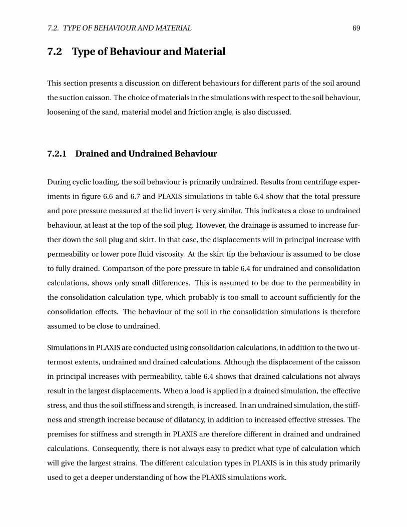
7.2. TYPE OF BEHAVIOUR AND MATERIAL 69
7.2 Type of Behaviour and Material
This section presents a discussion on different behaviours for different parts of the soil around
the suction caisson. The choice of materials in the simulations with respect to the soil behaviour,
loosening of the sand, material model and friction angle, is also discussed.
7.2.1 Drained and Undrained Behaviour
During cyclic loading, the soil behaviour is primarily undrained. Results from centrifuge exper-
iments in figure 6.6 and 6.7 and PLAXIS simulations in table 6.4 show that the total pressure
and pore pressure measured at the lid invert is very similar. This indicates a close to undrained
behaviour, at least at the top of the soil plug. However, the drainage is assumed to increase fur-
ther down the soil plug and skirt. In that case, the displacements will in principal increase with
permeability or lower pore fluid viscosity. At the skirt tip the behaviour is assumed to be close
to fully drained. Comparison of the pore pressure in table 6.4 for undrained and consolidation
calculations, shows only small differences. This is assumed to be due to the permeability in
the consolidation calculation type, which probably is too small to account sufficiently for the
consolidation effects. The behaviour of the soil in the consolidation simulations is therefore
assumed to be close to undrained.
Simulations in PLAXIS are conducted using consolidation calculations, in addition to the two ut-
termost extents, undrained and drained calculations. Although the displacement of the caisson
in principal increases with permeability, table 6.4 shows that drained calculations not always
result in the largest displacements. When a load is applied in a drained simulation, the effective
stress, and thus the soil stiffness and strength, is increased. In an undrained simulation, the stiff-
ness and strength increase because of dilatancy, in addition to increased effective stresses. The
premises for stiffness and strength in PLAXIS are therefore different in drained and undrained
calculations. Consequently, there is not always easy to predict what type of calculation which
will give the largest strains. The different calculation types in PLAXIS is in this study primarily
used to get a deeper understanding of how the PLAXIS simulations work.
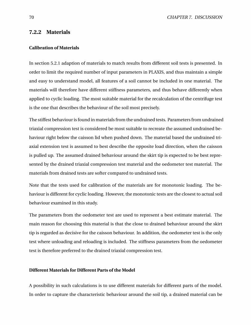
70 CHAPTER 7. DISCUSSION
7.2.2 Materials
Calibration of Materials
In section 5.2.1 adaption of materials to match results from different soil tests is presented. In
order to limit the required number of input parameters in PLAXIS, and thus maintain a simple
and easy to understand model, all features of a soil cannot be included in one material. The
materials will therefore have different stiffness parameters, and thus behave differently when
applied to cyclic loading. The most suitable material for the recalculation of the centrifuge test
is the one that describes the behaviour of the soil most precisely.
The stiffest behaviour is found in materials from the undrained tests. Parameters from undrained
triaxial compression test is considered be most suitable to recreate the assumed undrained be-
haviour right below the caisson lid when pushed down. The material based the undrained tri-
axial extension test is assumed to best describe the opposite load direction, when the caisson
is pulled up. The assumed drained behaviour around the skirt tip is expected to be best repre-
sented by the drained triaxial compression test material and the oedometer test material. The
materials from drained tests are softer compared to undrained tests.
Note that the tests used for calibration of the materials are for monotonic loading. The be-
haviour is different for cyclic loading. However, the monotonic tests are the closest to actual soil
behaviour examined in this study.
The parameters from the oedometer test are used to represent a best estimate material. The
main reason for choosing this material is that the close to drained behaviour around the skirt
tip is regarded as decisive for the caisson behaviour. In addition, the oedometer test is the only
test where unloading and reloading is included. The stiffness parameters from the oedometer
test is therefore preferred to the drained triaxial compression test.
Different Materials for Different Parts of the Model
A possibility in such calculations is to use different materials for different parts of the model.
In order to capture the characteristic behaviour around the soil tip, a drained material can be
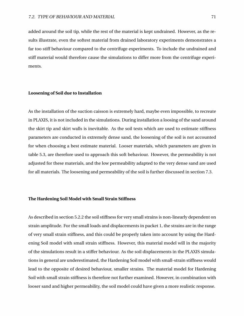
7.2. TYPE OF BEHAVIOUR AND MATERIAL 71
added around the soil tip, while the rest of the material is kept undrained. However, as the re-
sults illustrate, even the softest material from drained laboratory experiments demonstrates a
far too stiff behaviour compared to the centrifuge experiments. To include the undrained and
stiff material would therefore cause the simulations to differ more from the centrifuge experi-
ments.
Loosening of Soil due to Installation
As the installation of the suction caisson is extremely hard, maybe even impossible, to recreate
in PLAXIS, it is not included in the simulations. During installation a loosing of the sand around
the skirt tip and skirt walls is inevitable. As the soil tests which are used to estimate stiffness
parameters are conducted in extremely dense sand, the loosening of the soil is not accounted
for when choosing a best estimate material. Looser materials, which parameters are given in
table 5.3, are therefore used to approach this soft behaviour. However, the permeability is not
adjusted for these materials, and the low permeability adapted to the very dense sand are used
for all materials. The loosening and permeability of the soil is further discussed in section 7.3.
The Hardening Soil Model with Small Strain Stiffness
As described in section 5.2.2 the soil stiffness for very small strains is non-linearly dependent on
strain amplitude. For the small loads and displacements in packet 1, the strains are in the range
of very small strain stiffness, and this could be properly taken into account by using the Hard-
ening Soil model with small strain stiffness. However, this material model will in the majority
of the simulations result in a stiffer behaviour. As the soil displacements in the PLAXIS simula-
tions in general are underestimated, the Hardening Soil model with small-strain stiffness would
lead to the opposite of desired behaviour, smaller strains. The material model for Hardening
Soil with small strain stiffness is therefore not further examined. However, in combination with
looser sand and higher permeability, the soil model could have given a more realistic response.
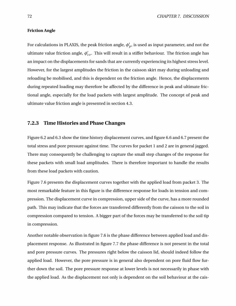
72 CHAPTER 7. DISCUSSION
Friction Angle
For calculations in PLAXIS, the peak friction angle, φ′p , is used as input parameter, and not the
ultimate value friction angle, φ′cv . This will result in a stiffer behaviour. The friction angle has
an impact on the displacements for sands that are currently experiencing its highest stress level.
However, for the largest amplitudes the friction in the caisson skirt may during unloading and
reloading be mobilised, and this is dependent on the friction angle. Hence, the displacements
during repeated loading may therefore be affected by the difference in peak and ultimate fric-
tional angle, especially for the load packets with largest amplitude. The concept of peak and
ultimate value friction angle is presented in section 4.3.
7.2.3 Time Histories and Phase Changes
Figure 6.2 and 6.3 show the time history displacement curves, and figure 6.6 and 6.7 present the
total stress and pore pressure against time. The curves for packet 1 and 2 are in general jagged.
There may consequently be challenging to capture the small step changes of the response for
these packets with small load amplitudes. There is therefore important to handle the results
from these load packets with caution.
Figure 7.6 presents the displacement curves together with the applied load from packet 3. The
most remarkable feature in this figure is the difference response for loads in tension and com-
pression. The displacement curve in compression, upper side of the curve, has a more rounded
path. This may indicate that the forces are transferred differently from the caisson to the soil in
compression compared to tension. A bigger part of the forces may be transferred to the soil tip
in compression.
Another notable observation in figure 7.6 is the phase difference between applied load and dis-
placement response. As illustrated in figure 7.7 the phase difference is not present in the total
and pore pressure curves. The pressures right below the caisson lid, should indeed follow the
applied load. However, the pore pressure is in general also dependent on pore fluid flow fur-
ther down the soil. The pore pressure response at lower levels is not necessarily in phase with
the applied load. As the displacement not only is dependent on the soil behaviour at the cais-
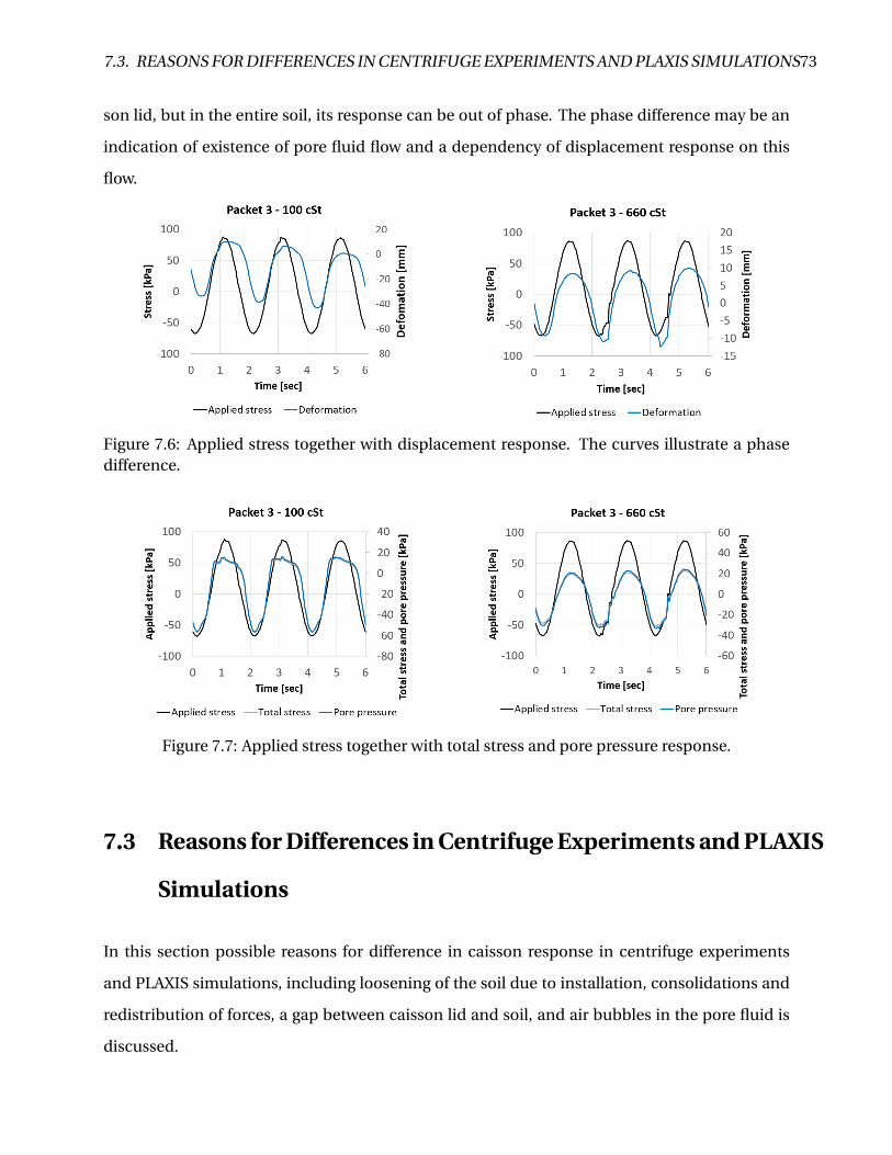
7.3. REASONS FOR DIFFERENCES IN CENTRIFUGE EXPERIMENTS AND PLAXIS SIMULATIONS73
son lid, but in the entire soil, its response can be out of phase. The phase difference may be an
indication of existence of pore fluid flow and a dependency of displacement response on this
flow.
Figure 7.6: Applied stress together with displacement response. The curves illustrate a phasedifference.
Figure 7.7: Applied stress together with total stress and pore pressure response.
7.3 Reasons for Differences in Centrifuge Experiments and PLAXIS
Simulations
In this section possible reasons for difference in caisson response in centrifuge experiments
and PLAXIS simulations, including loosening of the soil due to installation, consolidations and
redistribution of forces, a gap between caisson lid and soil, and air bubbles in the pore fluid is
discussed.
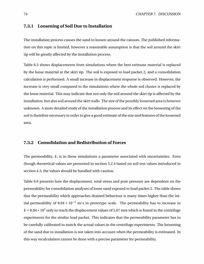
74 CHAPTER 7. DISCUSSION
7.3.1 Loosening of Soil Due to Installation
The installation process causes the sand to loosen around the caisson. The published informa-
tion on this topic is limited, however a reasonable assumption is that the soil around the skirt
tip will be greatly affected by the installation process.
Table 6.5 shows displacements from simulations where the best estimate material is replaced
by the loose material at the skirt tip. The soil is exposed to load packet 2, and a consolidation
calculation is performed. A small increase in displacement response is observed. However, the
increase is very small compared to the simulations where the whole soil cluster is replaced by
the loose material. This may indicate that not only the soil around the skirt tip is affected by the
installation, but also soil around the skirt walls. The size of the possibly loosened area is however
unknown. A more detailed study of the installation process and its effect on the loosening of the
soil is therefore necessary in order to give a good estimate of the size and features of the loosened
area.
7.3.2 Consolidation and Redistribution of Forces
The permeability, k, is in these simulations a parameter associated with uncertainties. Even
though theoretical values are presented in section 5.2.4 based on soil test values introduced in
section 4.3, the values should be handled with caution.
Table 6.6 presents how the displacement, total stress and pore pressure are dependent on the
permeability for consolidation analyses of loose sand exposed to load packet 2. The table shows
that the permeability which approaches drained behaviour is many times higher than the ini-
tial permeability of 8.04 × 10⁻³ m/s in prototype scale. The permeability has to increase to
k = 8.04×10² only to reach the displacement values of 5.07 mm which is found in the centrifuge
experiments for the similar load packet. This indicates that the permeability parameter has to
be carefully calibrated to match the actual values in the centrifuge experiments. The loosening
of the sand due to installation is not taken into account when the permeability is estimated. In
this way recalculation cannot be done with a precise parameter for permeability.
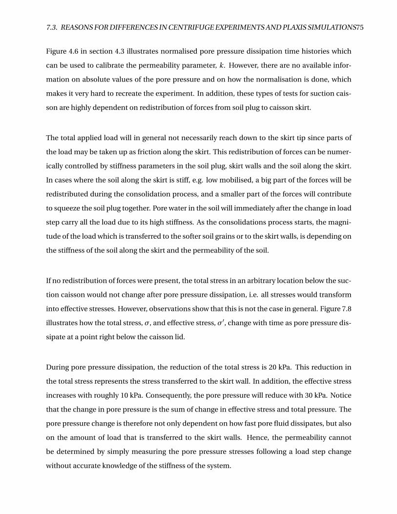
7.3. REASONS FOR DIFFERENCES IN CENTRIFUGE EXPERIMENTS AND PLAXIS SIMULATIONS75
Figure 4.6 in section 4.3 illustrates normalised pore pressure dissipation time histories which
can be used to calibrate the permeability parameter, k. However, there are no available infor-
mation on absolute values of the pore pressure and on how the normalisation is done, which
makes it very hard to recreate the experiment. In addition, these types of tests for suction cais-
son are highly dependent on redistribution of forces from soil plug to caisson skirt.
The total applied load will in general not necessarily reach down to the skirt tip since parts of
the load may be taken up as friction along the skirt. This redistribution of forces can be numer-
ically controlled by stiffness parameters in the soil plug, skirt walls and the soil along the skirt.
In cases where the soil along the skirt is stiff, e.g. low mobilised, a big part of the forces will be
redistributed during the consolidation process, and a smaller part of the forces will contribute
to squeeze the soil plug together. Pore water in the soil will immediately after the change in load
step carry all the load due to its high stiffness. As the consolidations process starts, the magni-
tude of the load which is transferred to the softer soil grains or to the skirt walls, is depending on
the stiffness of the soil along the skirt and the permeability of the soil.
If no redistribution of forces were present, the total stress in an arbitrary location below the suc-
tion caisson would not change after pore pressure dissipation, i.e. all stresses would transform
into effective stresses. However, observations show that this is not the case in general. Figure 7.8
illustrates how the total stress, σ, and effective stress, σ′, change with time as pore pressure dis-
sipate at a point right below the caisson lid.
During pore pressure dissipation, the reduction of the total stress is 20 kPa. This reduction in
the total stress represents the stress transferred to the skirt wall. In addition, the effective stress
increases with roughly 10 kPa. Consequently, the pore pressure will reduce with 30 kPa. Notice
that the change in pore pressure is the sum of change in effective stress and total pressure. The
pore pressure change is therefore not only dependent on how fast pore fluid dissipates, but also
on the amount of load that is transferred to the skirt walls. Hence, the permeability cannot
be determined by simply measuring the pore pressure stresses following a load step change
without accurate knowledge of the stiffness of the system.
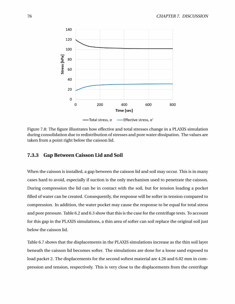
76 CHAPTER 7. DISCUSSION
Figure 7.8: The figure illustrates how effective and total stresses change in a PLAXIS simulationduring consolidation due to redistribution of stresses and pore water dissipation. The values aretaken from a point right below the caisson lid.
7.3.3 Gap Between Caisson Lid and Soil
When the caisson is installed, a gap between the caisson lid and soil may occur. This is in many
cases hard to avoid, especially if suction is the only mechanism used to penetrate the caisson.
During compression the lid can be in contact with the soil, but for tension loading a pocket
filled of water can be created. Consequently, the response will be softer in tension compared to
compression. In addition, the water pocket may cause the response to be equal for total stress
and pore pressure. Table 6.2 and 6.3 show that this is the case for the centrifuge tests. To account
for this gap in the PLAXIS simulations, a thin area of softer can soil replace the original soil just
below the caisson lid.
Table 6.7 shows that the displacements in the PLAXIS simulations increase as the thin soil layer
beneath the caisson lid becomes softer. The simulations are done for a loose sand exposed to
load packet 2. The displacements for the second softest material are 4.26 and 6.02 mm in com-
pression and tension, respectively. This is very close to the displacements from the centrifuge
7.3. REASONS FOR DIFFERENCES IN CENTRIFUGE EXPERIMENTS AND PLAXIS SIMULATIONS77
experiment with pore fluid viscosity 100 cSt which are 5.7 mm in compression and tension. The
softer layer beneath the caisson lid can be studied in a combination with changes in permeabil-
ity. A mix of these two elements may give response closer to the centrifuge experiments.
7.3.4 Air Bubbles in Pore Fluid
Another reason why the response in the simulations differ from the centrifuge experiments may
be that the pore fluid contains air bubbles. The fluid is in general very stiff, however air bubbles
make the fluid more compressible. In undrained triaxial tests a back pressure is applied to the
soil sample to reduce the size of the air bubbles. The stiffness of the soil increases with the back
pressure, but even with a very large pressure, there is hard to completely remove the air in the
fluid. In an experiment like the centrifuge experiment, air bubbles may presumably be present
in the pore fluid.
The air bubbles, and thus the soil, are assumed to be squeezed together when a cyclic com-
pression load is applied. A bigger part of the forces may therefore be taken by the skirt tip, and
consequently, the deformations will be larger compared to experiments with no air in the pore
fluid. In addition, the total stress and pore pressure response may become smaller due the re-
distribution of forces, as more of the loads are taken by the skirt tip and less is transferred to the
soil right beneath the caisson lid. As the simulations do not account for air bubbles in the pore
fluid, the bubbles can explain both the underestimated deformation and the overestimated total
stress and pore pressure response in the simulations.
Table 6.2 and 6.3 and figure 6.14 and 6.15 illustrate that the total stress and pore pressure in-
crease with permeability for centrifuge experiments. This strange behaviour may be explained
by air pockets in the pore fluid. A possibility is that the experiments with higher pore fluid vis-
cosity contain more air than the experiments with lower viscosity.
Air bubbles in the pore water can be accounted for in PLAXIS by reducing the Bulk modulus of
water, which will make the water softer. However, this is not further studied in this thesis. Note
that for the total stress and pore pressure the initial values from the centrifuge experiments are
unknown. This discussion is therefore solely based on cyclic peak amplitudes.
78 CHAPTER 7. DISCUSSION
7.3.5 Summary of Reasons for Difference in Centrifuge Experiments and PLAXIS
Simulations
In this section several reasons for different response in PLAXIS analyses and centrifuge exper-
iments are introduced, in which some of the theories have been tested using PLAXIS simula-
tions. Loosening of the soil material, calibration of permeability, gap between caisson lid and
soil and air bubbles in the pore fluid are mentioned. All of these arguments will presumably re-
sult in larger displacements and behaviour closer to the centrifuge experiments. An assumption
is therefore that a combination of several of the reasons given in this section will give the most
accurate behaviour, and lead to results from PLAXIS analyses more equal to centrifuge experi-
ments. This means that the whole gap between PLAXIS analyses and centrifuge tests does not
need to be covered by one parameter or property only.
7.4 Relevance of Centrifuge Experiments and Use of Data from
External Sources
A lot of elements need to be taken into account for experiments conducted in model scale, when
trying to adapt the results to prototype scale. As for centrifuge experiments, the soil stresses
are similar those of the prototype, which makes the adaption a bit easier. However, the use of
smaller dimensions may be challenging in order to capture all the features of a prototype model
precisely. The use of a 0.5 mm skirt wall thickness in the centrifuge test, may, for instance, intro-
duce a scale effect as it changes the ratio between skirt wall thickness and grain size compared
to prototype conditions.
The soil sample used during the centrifuge experiments are very dense, which is typical for
North Sea sands. However, during installation parts of the soil around the suction caisson may
become looser, and this should be taken into account. Soil parameters measured in very dense
sand may therefore differ from what is actually present in the soil samples after installation.
7.4. RELEVANCE OF CENTRIFUGE EXPERIMENTS AND USE OF DATA FROM EXTERNAL SOURCES79
The centrifuge experiment has used one single suction caisson to represent one of the caissons
in a tripod foundation. Even though several types of loading sequences have been applied to the
caisson, the interaction between the caissons, such as dependency on distance between them,
cannot be estimated from the centrifuge experiments examined in this study.
The data from the centrifuge experiments are collected from sources at the UWA. As the experi-
ments have been conducted by a third party, information about how the experiments have been
carried out is limited to what is written and published. This leads to less knowledge of how suc-
cessful or trustful the experiments and results are. By not having this information the risk of
misinterpreting the results from the experiments increases.

Chapter 8
Conclusion and Recommendations for
Further Work
8.1 Summary and Conclusion
This thesis has examined the response of offshore wind tribunes with respect to cyclic loading.
Offshore installations are in general subject to cyclic loading due to wind, waves and currents.
However, compared to traditional and heavy offshore installations in the oil and gas industry,
offshore wind turbines are more susceptible to cyclic loading. Thus, the cyclic behaviour of
sand is of key importance to this thesis.
The thesis is seen in light of the theory on cyclic response of suction caissons and the HCA
model. During cyclic loading, a combination of average loads and a large number of small-
strain cyclic loads will cause the soil to accumulate pore pressure or deformation, or both. The
HCA model, described in this thesis, accounts for these effects by using an explicit calculation
strategy which calculates the accumulation directly. Implicit calculation is performed in order
to update the strain amplitude after a large number of cycles. The accumulation is given by six
independent functions.
The UWA has conducted several centrifuge experiments on very dense Baskarp sand. The ex-
periments aim to represent one of three suction caissons supporting an offshore wind turbine
81
82 CHAPTER 8. CONCLUSION AND RECOMMENDATIONS FOR FURTHER WORK
in the North Sea. In order to make the experiments as realistic as possible the caisson is installed
using suction. The installation is followed by cyclic loading, and the response of the caisson is
investigated.
When it comes to the first objective of the thesis, the results examined from the centrifuge exper-
iments performed at the UWA demonstrate a significant difference in response for compression
and tension loading. This is in this master thesis discussed to be due to a softer behaviour in
tension. Experiments with different pore fluid viscosity is conducted and the effect of drainage
is investigated in the thesis. As the experiments with lowest pore fluid viscosity result in the
largest displacements, the drainage is assumed to affect the results. An observed phase differ-
ence in the response support this assumption.
Regarding the second objective of the thesis, the recalculation of the centrifuge experiments
illustrates the challenge of simulating the complex caisson behaviour. Even though material pa-
rameters calibrated from oedometer tests are assumed to best estimate the caisson response,
simulations using a looser material are closest to recreate the response from the centrifuge
experiments. However, even with a loose material, the displacements are in the simulations
mainly underestimated, while the total stress and pore pressure are overestimated.
The different response in the centrifuge experiments compared to the simulations are assumed
to be due to loosening of the sand during installation, limitations in calibration of the perme-
ability parameter, redistribution of forces, water pocket beneath the caisson or air bubbles in the
pore fluid. The difference may be caused by one single or a combination of the aforementioned
reasons.
8.2 Recommendations for Further Work
Based on the thesis the following recommendations for further work are proposed.
Input parameters in the PLAXIS simulations are not based on proper sand specified cyclic lab-
oratory tests. A more precise estimation of the parameters is recommended for further studies.
The permeability is of special importance and a better system to calibrate this parameter should
8.2. RECOMMENDATIONS FOR FURTHER WORK 83
be developed. A possibility is to measure the amount of dissipated pore fluid during installation
or perform a steady state seepage analysis after installation.
It would also be advantageous to perform a more idealised test to calibrate interface friction
between the sand and aluminium caisson. A pull-out test of a simple aluminium plate will result
in interface parameters that are not so heavily dependent on initial stresses as the extraction
resistance tests performed in connection with the centrifuge experiments. To calibrate the effect
of loosening of sand due to the installation process, a reference test where the caisson is installed
in loose can be performed. Comparison of results from experiments with dense sand will give
an indication of the extent of the loosened area.
The installation of the caisson in the centrifuge experiments is performed by suction only. Con-
sequently, there is a major risk of existence of a water pocket beneath the caisson lid. Further
experiments should avoid this problem either by covering the pocket with fill dirt, which is often
done in practice, or by pushing the caisson into the seabed instead of just pulling.
For further analyses in PLAXIS or other simulation programs the initial value of the total stress
and pore pressure should be known. This is useful to make sure the response of the simulations
matches the centrifuge experiments. In addition, simulations using a lower Bulk modulus for
water to investigate the hypothesis of air bubbles in the water would be of great interest.
The accumulated effects due to cyclic loads are very important for suction caissons supporting
offshore wind turbines. It will be highly interesting to study these effects in a computer simu-
lation software, such as PLAXIS. At NGI, the HCA model is already implemented into PLAXIS.
Recalculation of the centrifuge experiments by the use of this model will be of great value, espe-
cially as the long-term effects of cyclic loads can be predicted in this model.

List of Figures
2.1 Seepage flow with upward gradient on the inside and downward gradient on the
outside the caisson caused by suction pressure during installation (Bienen et al.,
2018b). . . . . . . . . . . . . . . . . . . . . . . . . . . . . . . . . . . . . . . . . . . . . . 6
2.2 The figure illustrates how the load direction is decisive for what kind of loads the
different caissons will experience (Bienen et al., 2018a). . . . . . . . . . . . . . . . . 9
2.3 A top view of three caissons supporting an offshore wind turbine (Bienen et al.,
2018b). . . . . . . . . . . . . . . . . . . . . . . . . . . . . . . . . . . . . . . . . . . . . . 9
3.1 The basic idea of a combined implicit and explicit calculation. The horizontal axis
is time, t , for implicit calculations and number of cycles, N , for explicit calcula-
tions (Niemunis et al., 2005). . . . . . . . . . . . . . . . . . . . . . . . . . . . . . . . . 15
4.1 Illustration of the model caisson, equipment and arrangement used during testing
at UWA (Bienen et al., 2018b). . . . . . . . . . . . . . . . . . . . . . . . . . . . . . . . . 20
4.2 The applied cyclic loading aim to represent loads from an offshore wind turbine at
40 m water depth in the North Sea (Bienen et al., 2018b). . . . . . . . . . . . . . . . . 21
4.3 The testing procedure of the experiments at UWA schematically presented (Bienen
et al., 2018b). . . . . . . . . . . . . . . . . . . . . . . . . . . . . . . . . . . . . . . . . . . 21
4.4 The grain-size distribution of Baskarp sand is similar to typical North Sea sands
(adapted from Andersen (1989)). . . . . . . . . . . . . . . . . . . . . . . . . . . . . . . 22
4.5 Definition of peak friction angle, φ′p , and ultimate friction angle, φ′
cv , in drained
tests on loose and dense sands (Andersen and Schjetne, 2012). . . . . . . . . . . . . 23
85
86 LIST OF FIGURES
4.6 Difference in consolidation characteristics for the two pore fluids. The horizon-
tal axis represents time in seconds on a logarithmic scale, while the vertical axis
illustrates normalised pore pressure (Bienen et al., 2018b). . . . . . . . . . . . . . . 23
5.1 A screenshot shows the caisson of the PLAXIS model used in the PLAXIS simulations. 26
5.2 A screenshot shows a triangle added to the bottom of the caisson skirt to account
for the thickness of the skirt. The triangle is 5 cm at the bottom. . . . . . . . . . . . 26
5.3 The dependency of element size on displacement. “Very fine” and “very coarse”
element distributions are shown in the figure. . . . . . . . . . . . . . . . . . . . . . . 27
5.4 The figure shows the points around the skirt tip which contribute to refining of the
mesh. . . . . . . . . . . . . . . . . . . . . . . . . . . . . . . . . . . . . . . . . . . . . . . 28
5.5 An overview of the mesh used in the calculations. . . . . . . . . . . . . . . . . . . . . 28
5.6 A cluster representing another material around the skirt tip. . . . . . . . . . . . . . . 29
5.7 A thin layer of another material representing a water pocket just beneath the cais-
son lid. . . . . . . . . . . . . . . . . . . . . . . . . . . . . . . . . . . . . . . . . . . . . . 29
5.8 Exact position of displacement node and stress point. . . . . . . . . . . . . . . . . . 30
5.9 A comparison between oedometer test from experiments and SoilTest in PLAXIS.
Stiffness parameters for the hardening soil material used in PLAXIS are shown in
table 5.2. . . . . . . . . . . . . . . . . . . . . . . . . . . . . . . . . . . . . . . . . . . . . 33
5.10 A comparison between triaxial drained compression test from experiments and
SoilTest in PLAXIS. Stiffness parameters for the hardening soil material used in
PLAXIS are shown in table 5.2. . . . . . . . . . . . . . . . . . . . . . . . . . . . . . . . 33
5.11 A comparison between triaxial undrained compression test from experiments and
SoilTest in PLAXIS. Stiffness parameters for the hardening soil material used in
PLAXIS are shown in table 5.2. . . . . . . . . . . . . . . . . . . . . . . . . . . . . . . . 34
5.12 A comparison between triaxial undrained extension test from experiments and
SoilTest in PLAXIS. Stiffness parameters for the hardening soil material used in
PLAXIS are shown in table 5.2. . . . . . . . . . . . . . . . . . . . . . . . . . . . . . . . 34
5.13 Non-linearly dependency of soil stiffness on strain amplitude (Brinkgreve et al.,
2017). . . . . . . . . . . . . . . . . . . . . . . . . . . . . . . . . . . . . . . . . . . . . . . 35
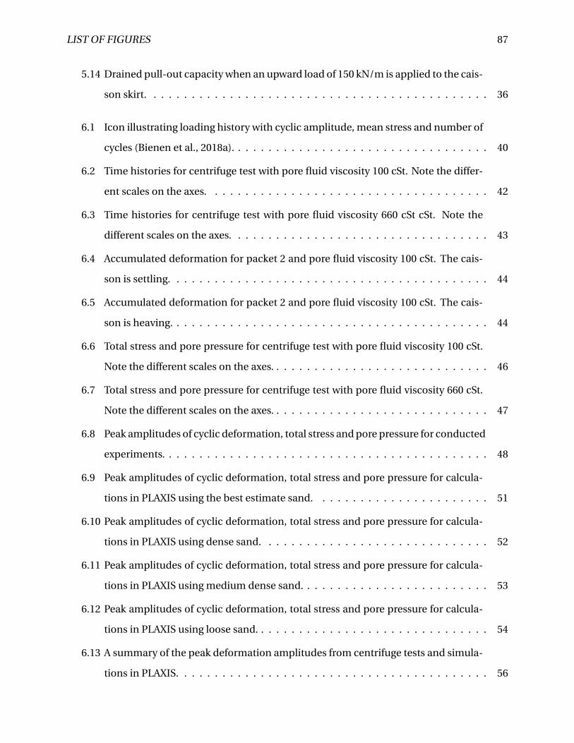
LIST OF FIGURES 87
5.14 Drained pull-out capacity when an upward load of 150 kN/m is applied to the cais-
son skirt. . . . . . . . . . . . . . . . . . . . . . . . . . . . . . . . . . . . . . . . . . . . . 36
6.1 Icon illustrating loading history with cyclic amplitude, mean stress and number of
cycles (Bienen et al., 2018a). . . . . . . . . . . . . . . . . . . . . . . . . . . . . . . . . . 40
6.2 Time histories for centrifuge test with pore fluid viscosity 100 cSt. Note the differ-
ent scales on the axes. . . . . . . . . . . . . . . . . . . . . . . . . . . . . . . . . . . . . 42
6.3 Time histories for centrifuge test with pore fluid viscosity 660 cSt cSt. Note the
different scales on the axes. . . . . . . . . . . . . . . . . . . . . . . . . . . . . . . . . . 43
6.4 Accumulated deformation for packet 2 and pore fluid viscosity 100 cSt. The cais-
son is settling. . . . . . . . . . . . . . . . . . . . . . . . . . . . . . . . . . . . . . . . . . 44
6.5 Accumulated deformation for packet 2 and pore fluid viscosity 100 cSt. The cais-
son is heaving. . . . . . . . . . . . . . . . . . . . . . . . . . . . . . . . . . . . . . . . . . 44
6.6 Total stress and pore pressure for centrifuge test with pore fluid viscosity 100 cSt.
Note the different scales on the axes. . . . . . . . . . . . . . . . . . . . . . . . . . . . . 46
6.7 Total stress and pore pressure for centrifuge test with pore fluid viscosity 660 cSt.
Note the different scales on the axes. . . . . . . . . . . . . . . . . . . . . . . . . . . . . 47
6.8 Peak amplitudes of cyclic deformation, total stress and pore pressure for conducted
experiments. . . . . . . . . . . . . . . . . . . . . . . . . . . . . . . . . . . . . . . . . . . 48
6.9 Peak amplitudes of cyclic deformation, total stress and pore pressure for calcula-
tions in PLAXIS using the best estimate sand. . . . . . . . . . . . . . . . . . . . . . . 51
6.10 Peak amplitudes of cyclic deformation, total stress and pore pressure for calcula-
tions in PLAXIS using dense sand. . . . . . . . . . . . . . . . . . . . . . . . . . . . . . 52
6.11 Peak amplitudes of cyclic deformation, total stress and pore pressure for calcula-
tions in PLAXIS using medium dense sand. . . . . . . . . . . . . . . . . . . . . . . . . 53
6.12 Peak amplitudes of cyclic deformation, total stress and pore pressure for calcula-
tions in PLAXIS using loose sand. . . . . . . . . . . . . . . . . . . . . . . . . . . . . . . 54
6.13 A summary of the peak deformation amplitudes from centrifuge tests and simula-
tions in PLAXIS. . . . . . . . . . . . . . . . . . . . . . . . . . . . . . . . . . . . . . . . . 56
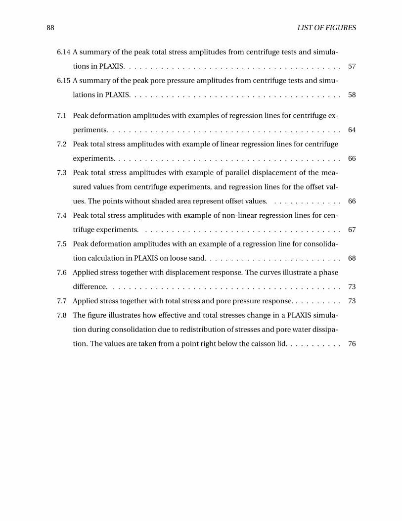
88 LIST OF FIGURES
6.14 A summary of the peak total stress amplitudes from centrifuge tests and simula-
tions in PLAXIS. . . . . . . . . . . . . . . . . . . . . . . . . . . . . . . . . . . . . . . . . 57
6.15 A summary of the peak pore pressure amplitudes from centrifuge tests and simu-
lations in PLAXIS. . . . . . . . . . . . . . . . . . . . . . . . . . . . . . . . . . . . . . . . 58
7.1 Peak deformation amplitudes with examples of regression lines for centrifuge ex-
periments. . . . . . . . . . . . . . . . . . . . . . . . . . . . . . . . . . . . . . . . . . . . 64
7.2 Peak total stress amplitudes with example of linear regression lines for centrifuge
experiments. . . . . . . . . . . . . . . . . . . . . . . . . . . . . . . . . . . . . . . . . . . 66
7.3 Peak total stress amplitudes with example of parallel displacement of the mea-
sured values from centrifuge experiments, and regression lines for the offset val-
ues. The points without shaded area represent offset values. . . . . . . . . . . . . . 66
7.4 Peak total stress amplitudes with example of non-linear regression lines for cen-
trifuge experiments. . . . . . . . . . . . . . . . . . . . . . . . . . . . . . . . . . . . . . 67
7.5 Peak deformation amplitudes with an example of a regression line for consolida-
tion calculation in PLAXIS on loose sand. . . . . . . . . . . . . . . . . . . . . . . . . . 68
7.6 Applied stress together with displacement response. The curves illustrate a phase
difference. . . . . . . . . . . . . . . . . . . . . . . . . . . . . . . . . . . . . . . . . . . . 73
7.7 Applied stress together with total stress and pore pressure response. . . . . . . . . . 73
7.8 The figure illustrates how effective and total stresses change in a PLAXIS simula-
tion during consolidation due to redistribution of stresses and pore water dissipa-
tion. The values are taken from a point right below the caisson lid. . . . . . . . . . . 76
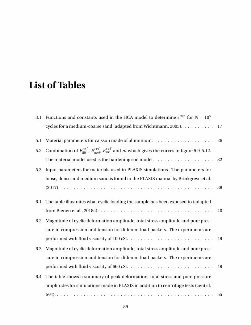
List of Tables
3.1 Functions and constants used in the HCA model to determine εacc for N = 105
cycles for a medium-coarse sand (adapted from Wichtmann, 2005). . . . . . . . . . 17
5.1 Material parameters for caisson made of aluminium. . . . . . . . . . . . . . . . . . . 26
5.2 Combination of E r e f50 , E r e f
oed , E r e fur and m which gives the curves in figure 5.9-5.12.
The material model used is the hardening soil model. . . . . . . . . . . . . . . . . . 32
5.3 Input parameters for materials used in PLAXIS simulations. The parameters for
loose, dense and medium sand is found in the PLAXIS manual by Brinkgreve et al.
(2017). . . . . . . . . . . . . . . . . . . . . . . . . . . . . . . . . . . . . . . . . . . . . . 38
6.1 The table illustrates what cyclic loading the sample has been exposed to (adapted
from Bienen et al., 2018a). . . . . . . . . . . . . . . . . . . . . . . . . . . . . . . . . . . 40
6.2 Magnitude of cyclic deformation amplitude, total stress amplitude and pore pres-
sure in compression and tension for different load packets. The experiments are
performed with fluid viscosity of 100 cSt. . . . . . . . . . . . . . . . . . . . . . . . . . 49
6.3 Magnitude of cyclic deformation amplitude, total stress amplitude and pore pres-
sure in compression and tension for different load packets. The experiments are
performed with fluid viscosity of 660 cSt. . . . . . . . . . . . . . . . . . . . . . . . . . 49
6.4 The table shows a summary of peak deformation, total stress and pore pressure
amplitudes for simulations made in PLAXIS in addition to centrifuge tests (centrif.
test). . . . . . . . . . . . . . . . . . . . . . . . . . . . . . . . . . . . . . . . . . . . . . . . 55
89
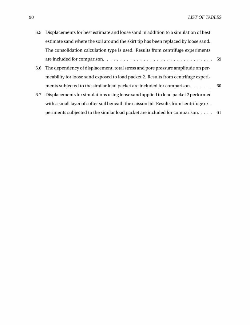
90 LIST OF TABLES
6.5 Displacements for best estimate and loose sand in addition to a simulation of best
estimate sand where the soil around the skirt tip has been replaced by loose sand.
The consolidation calculation type is used. Results from centrifuge experiments
are included for comparison. . . . . . . . . . . . . . . . . . . . . . . . . . . . . . . . . 59
6.6 The dependency of displacement, total stress and pore pressure amplitude on per-
meability for loose sand exposed to load packet 2. Results from centrifuge experi-
ments subjected to the similar load packet are included for comparison. . . . . . . 60
6.7 Displacements for simulations using loose sand applied to load packet 2 performed
with a small layer of softer soil beneath the caisson lid. Results from centrifuge ex-
periments subjected to the similar load packet are included for comparison. . . . . 61
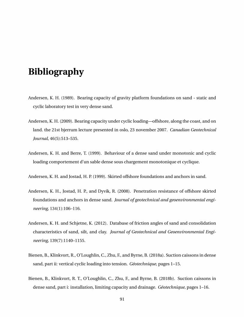
Bibliography
Andersen, K. H. (1989). Bearing capacity of gravity platform foundations on sand - static and
cyclic laboratory test in very dense sand.
Andersen, K. H. (2009). Bearing capacity under cyclic loading—offshore, along the coast, and on
land. the 21st bjerrum lecture presented in oslo, 23 november 2007. Canadian Geotechnical
Journal, 46(5):513–535.
Andersen, K. H. and Berre, T. (1999). Behaviour of a dense sand under monotonic and cyclic
loading comportement d’un sable dense sous chargement monotonique et cyclique.
Andersen, K. H. and Jostad, H. P. (1999). Skirted offshore foundations and anchors in sand.
Andersen, K. H., Jostad, H. P., and Dyvik, R. (2008). Penetration resistance of offshore skirted
foundations and anchors in dense sand. Journal of geotechnical and geoenvironmental engi-
neering, 134(1):106–116.
Andersen, K. H. and Schjetne, K. (2012). Database of friction angles of sand and consolidation
characteristics of sand, silt, and clay. Journal of Geotechnical and Geoenvironmental Engi-
neering, 139(7):1140–1155.
Bienen, B., Klinkvort, R., O’Loughlin, C., Zhu, F., and Byrne, B. (2018a). Suction caissons in dense
sand, part ii: vertical cyclic loading into tension. Géotechnique, pages 1–15.
Bienen, B., Klinkvort, R. T., O’Loughlin, C., Zhu, F., and Byrne, B. (2018b). Suction caissons in
dense sand, part i: installation, limiting capacity and drainage. Géotechnique, pages 1–16.
91
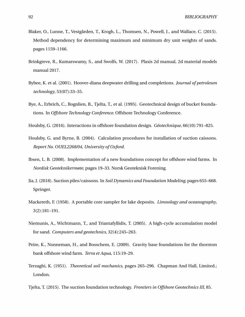
92 BIBLIOGRAPHY
Blaker, O., Lunne, T., Vestgården, T., Krogh, L., Thomsen, N., Powell, J., and Wallace, C. (2015).
Method dependency for determining maximum and minimum dry unit weights of sands.
pages 1159–1166.
Brinkgreve, R., Kumarswamy, S., and Swolfs, W. (2017). Plaxis 2d manual, 2d material models
manual 2017.
Bybee, K. et al. (2001). Hoover-diana deepwater drilling and completions. Journal of petroleum
technology, 53(07):33–35.
Bye, A., Erbrich, C., Rognlien, B., Tjelta, T., et al. (1995). Geotechnical design of bucket founda-
tions. In Offshore Technology Conference. Offshore Technology Conference.
Houlsby, G. (2016). Interactions in offshore foundation design. Géotechnique, 66(10):791–825.
Houlsby, G. and Byrne, B. (2004). Calculation procedures for installation of suction caissons.
Report No. OUEL2268/04, University of Oxford.
Ibsen, L. B. (2008). Implementation of a new foundations concept for offshore wind farms. In
Nordisk Geoteknikermøte, pages 19–33. Norsk Geoteknisk Forening.
Jia, J. (2018). Suction piles/caissons. In Soil Dynamics and Foundation Modeling, pages 655–668.
Springer.
Mackereth, F. (1958). A portable core sampler for lake deposits. Limnology and oceanography,
3(2):181–191.
Niemunis, A., Wichtmann, T., and Triantafyllidis, T. (2005). A high-cycle accumulation model
for sand. Computers and geotechnics, 32(4):245–263.
Peire, K., Nonneman, H., and Bosschem, E. (2009). Gravity base foundations for the thornton
bank offshore wind farm. Terra et Aqua, 115:19–29.
Terzaghi, K. (1951). Theoretical soil mechanics, pages 265–296. Chapman And Hall, Limited.;
London.
Tjelta, T. (2015). The suction foundation technology. Frontiers in Offshore Geotechnics III, 85.
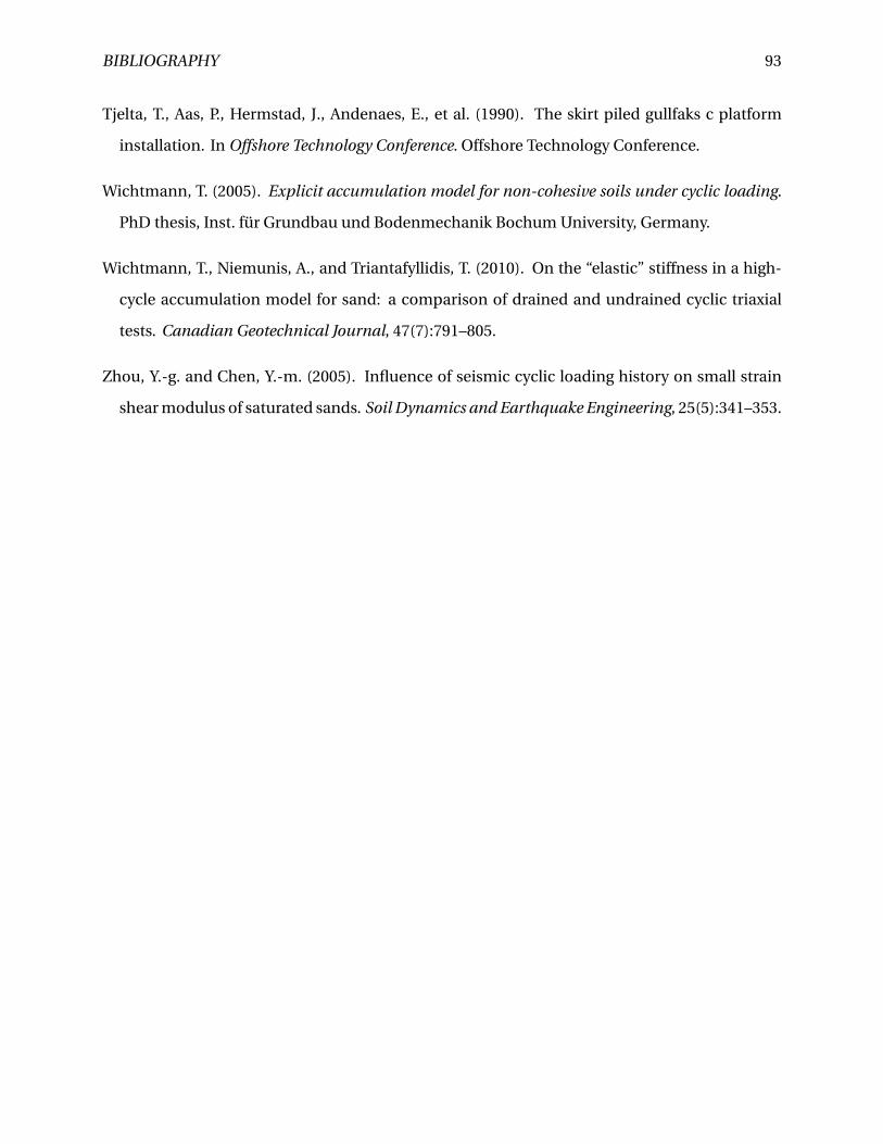
BIBLIOGRAPHY 93
Tjelta, T., Aas, P., Hermstad, J., Andenaes, E., et al. (1990). The skirt piled gullfaks c platform
installation. In Offshore Technology Conference. Offshore Technology Conference.
Wichtmann, T. (2005). Explicit accumulation model for non-cohesive soils under cyclic loading.
PhD thesis, Inst. für Grundbau und Bodenmechanik Bochum University, Germany.
Wichtmann, T., Niemunis, A., and Triantafyllidis, T. (2010). On the “elastic” stiffness in a high-
cycle accumulation model for sand: a comparison of drained and undrained cyclic triaxial
tests. Canadian Geotechnical Journal, 47(7):791–805.
Zhou, Y.-g. and Chen, Y.-m. (2005). Influence of seismic cyclic loading history on small strain
shear modulus of saturated sands. Soil Dynamics and Earthquake Engineering, 25(5):341–353.