1

Finite element analysis of a steel conoid shell P.C.J. Hoogenboom, 23 May 2018 Install SCIA Engineer on your computer. You can download the software for free from http://www.scia-campus.com .

2

Choosing the functionality makes extra menu items visible.

Every finite element program consists of three parts. 1) Drawing the structure (pre-processing) 2) Performing the analysis 3) Displaying the results (post-processing) The project tree (“main” window) shows these steps and extra sub steps. More steps will become visible when an analysis has been performed.

3

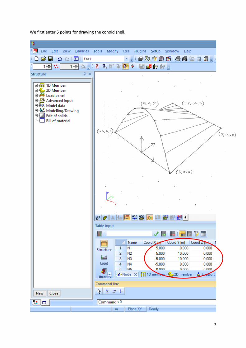
We first enter 5 points for drawing the conoid shell.

4

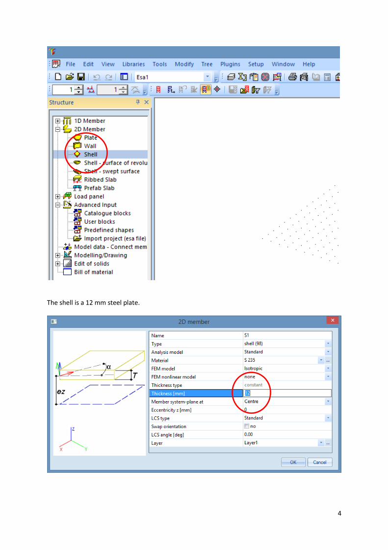
The shell is a 12 mm steel plate.

5

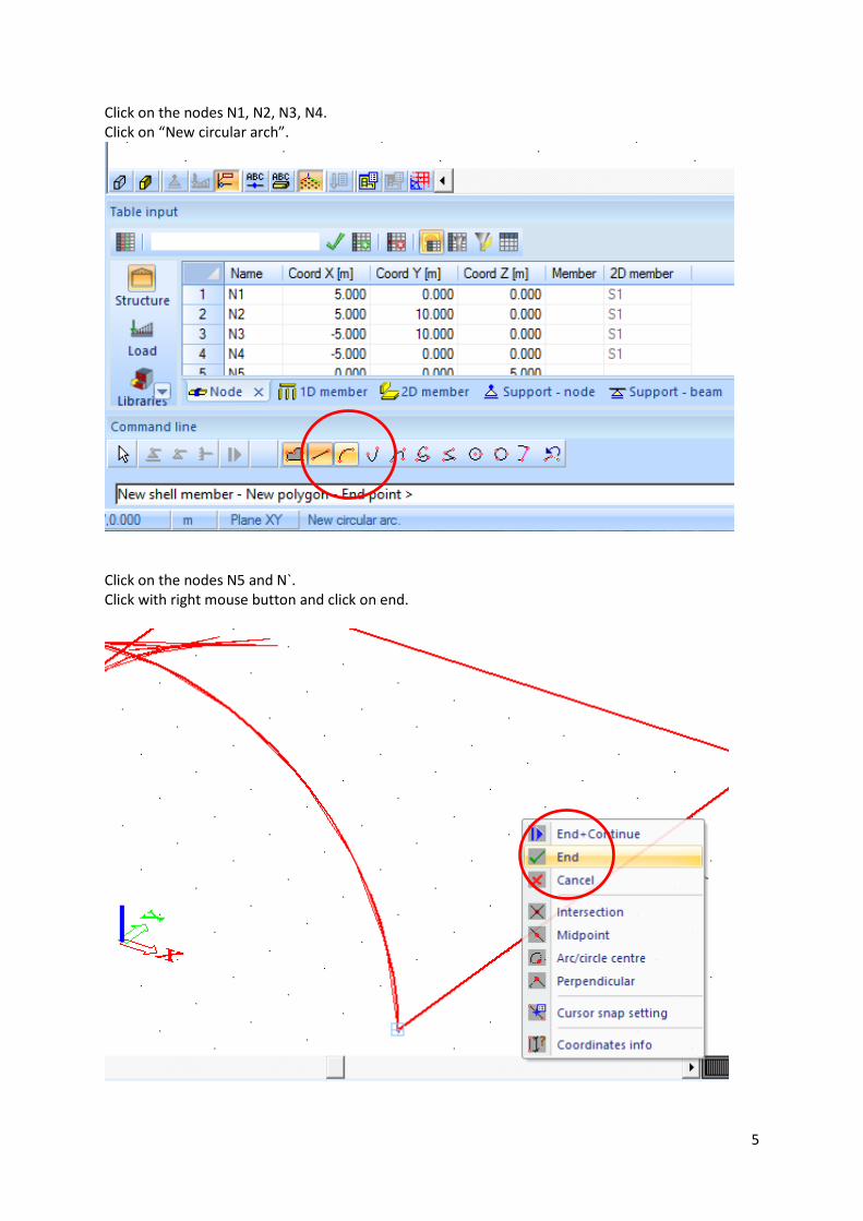
Click on the nodes N1, N2, N3, N4. Click on “New circular arch”.

Click on the nodes N5 and N`. Click with right mouse button and click on end.

6

The shell is supported by fixing the straight edges.

Click on the straight edges.

7

Click with the right mouse button and click end. One load case is already present: Self-weight. We add a load case: Snow.

8

LG1

9

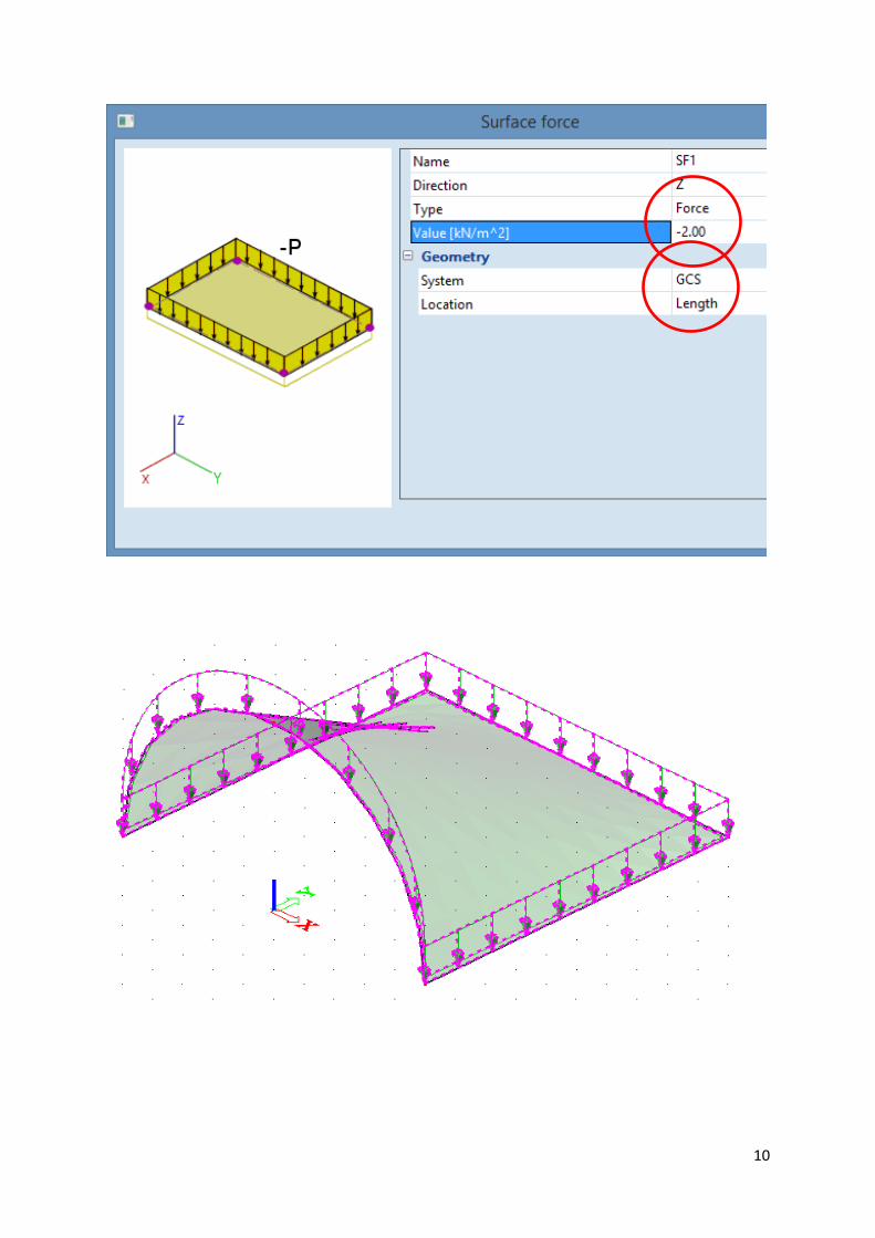
Now we can enter the snow load: 2 kN/m2

10

11

We make a load combinations in which both Self-weight and Snow occur at the same time. (Safety factors are not used.)

12

We first perform a linear elastic analysis.

The influence length is 2.4*sqrt(5*0.012) = 0.6 m. The element size should be 1/6 of this. Let’s set the element size to 0.3 m. This is a bit large but we can always make it smaller later.

13

Note that the software has checked equilibrium of the loads and the support reactions. If this would not be OK the arithmetic accuracy would not be OK. Let’s look at the results.

Deflection due to the load combination.

14

The deflection is largest in the flat part of the shell. Nonetheless it is just 2.2 mm which is surely acceptable. The mesh is shown too. The elements may be too large to describe the red peak accurately. For now we leave the element size as it is because we do not want to increase the computation time. Note that the mesh consists of rectangles and triangles. Triangles are less accurate than rectangles. Why does the program choose triangles?

15

Let’s look at the Von Mises stresses.

In the picture below the mesh is not displayed. This can be selected in “Drawing setup 2D”.

In most of the shell the stress is almost zero. The largest stresses occur at the edges (edge disturbance). A largest stress of 20.5 N/mm2 is not much. But this will increase when the mesh is refined. Nonetheless, perhaps the shell can be designed much thinner. This view is at the inside surface of the shell. If you turn the shell around you can see the stresses at the outside surface of the shell.

16

Let’s reduce the element size to check the accuracy. Element size: 0.300 m 0.150 m Largest Von Mises stress 20.5 N/mm2 20.9 N/mm2 The new linear elastic calculation takes a few minutes. The difference between the two computations is just 0.4 N/mm2. So an estimate of the error that we make with the 0.150 mm mesh is 0.4 N/mm2 or 2% which is sufficiently small for most applications. In the following we will work with 0.300 m elements. Let’s check buckling. Now we need to define stability load combinations.

(The teacher does not understand why the software does not use the normal load combinations for stability analysis too. Perhaps this extra step will be removed in future software versions.)

17

Now we can perform the linear buckling analysis. Let’s compute 6 buckling modes.

18

Let’s look at the results.

First buckling mode:

It buckles in this shape when the load combination is multiplied with a load factor of 8.28. The subsequent buckling load factors are 8.33, 11.43, 11.79, 12.50, 12.99 et cetera. If you want to know more bucking load factors than you can select this just before starting the buckling analysis. The figure shows that this buckling mode moves mostly outwards. However, the exact same mode is sometimes displayed as moving mostly inwards. Does this make sense?

19

Clearly, an edge beam would prevent most buckling modes. With an edge beam the shell could be even thinner. Let’s look at the natural frequencies. First we need to add mass to the load cases. (The program already knows about the mass of the materials but it does not know whether other loads have a mass. For example snow load has a mass and wind load has no mass.) Let’s study the shell without any extra mass. The mass of the materials is in something called MG1.

20

We make a mass combination of just this mass.

Now we can compute the natural frequencies.

21

Let’s look at the results.

The first vibration mode: The natural frequency is 8.68 Hz.

The subsequent natural frequencies are 8.68, 12.61, 12.76, 15.38, 15.83, 16.39, 17.05, 18.22, 20.07 et cetera. Note that there is little space between the natural frequencies. This is typical for shell structures. Frame structures are sometimes designed such that the frequency of the load is no problem because it is in between two natural frequencies. Is this possible for shells too? The program has computed the 10 smallest natural frequencies. If you want to see more you can set this just before starting the computation.

22

This shell is not sensitive to wind loading because wind gusts have a frequency of approximately 1 Hz or smaller. This shell is sensitive to earthquakes. It would not be sensitive to earthquakes if all natural frequencies were larger than 10 Hz. Vibration mode shapes often look like buckling mode shapes. There is a situation in which they are exactly the same. This is when the load is so large that the structure almost buckles. If you give the structure is little push it moves away slowly and comes back slowly. In this situation the natural frequency is almost zero and the vibration mode shape is the same as the buckling mode shape. Why does the program always perform linear analyses before computing natural frequencies? Let’s do a nonlinear analysis. First we need to specify nonlinear combinations. (The teacher thinks that there is no difference between linear and nonlinear load combinations.) Here we can specify a shape imperfection. We choose the first buckling mode as imperfection with an amplitude of 24 mm (2 times the shell thickness).

23

We also apply the imperfection in the other direction. So an amplitude of -24 mm.

The software applies the load in 10 equal steps (increments). After each step it uses the Newton-Raphson method to compute the displacements. This involves a few iterations until sufficient accuracy is obtained. The program would stop prematurely if more than 100 iterations have been performed without finding sufficient accuracy.

24

During the computation the load displacement diagram is shown. The pink curve shows the displacement of node 5. The blue curve shows the rotation of node 55, which apparently is the node with the largest rotation. The curve is not smooth because the results for all iterations are shown and not only the ones that are accurate.

25

The imperfection with an amplitude of -24 mm gives the largest deflection.

Compare the deflection of the linear analysis to that of the nonlinear analysis. What causes the differences? The Von Mises stress is largest for the imperfection with an amplitude of 24 mm. However, it is still very small.

26

Let’s see if the load factor of the linear buckling analysis is correct. We increase the loads with a factor 8.28. This is the buckling load factor computed in the linear buckling analysis.

We apply the load in 80 increments.

27

For the amplitude of 24 mm the Newton-Raphson procedure diverges at load increment 44. The load factor is then 44/80 x 8.28 = 4.55. The deflection is then 125 mm. Often, this is the maximum load. We need to assume that the shell buckles at this load. For the amplitude of -24 mm the Newton-Raphson procedure diverges at load increment 69. The load factor is then 69/80 x 8.28 = 7.14. This shell is sensitive to shape imperfections but not very sensitive. This design can be improved: The thickness can be reduced. If an edge beam is added the thickness can be reduced even further.