Abstract—This article presents the solution of boundary

value problems using finite difference scheme and Laplace

transform method. Some examples are solved to illustrate the

methods; Laplace transforms gives a closed form solution while

in finite difference scheme the extended interval enhances the

convergence of the solution.

Index Terms— Finite difference method, Laplace

transforms, boundary value problems

I. INTRODUCTION

wo-point boundary value problems have received a

considerable attention due to its importance in many

areas of sciences and engineering. These types of differential

equations arise very frequently in fluid mechanics, quantum

mechanics, optimal control, chemical-reactor theory,

aerodynamics, reaction-diffusion process and geophysics.

Various analytical and numerical techniques proposed for

the solution of differential equations are available in

literature; some of these are Differential Transform Method

[1-6], Rung-Kutta 4th

Order Method [7], Bernoulli

Polynomials [8], Cubic Spline Method [9], Sinc Collocation

Method [10], Modified Picard Technique [11], Block

Method [12-14], Adomian Decomposition Method [15-20],

Homotopy Perturbation Method [21-23].

In this work, finite difference method proposed for the

solution of two-point boundary value problems has been

widely applied [24-26]. However, in this article the step

length is extended and it is observed that the approach

enhances the convergence of the result when compared with

the exact from Laplace transforms (which gives a close form

of solution), See Tables 1 and 2.

.

Manuscript received February 13, 2017; revised March 10, 2017. This

work was supported by Centre for Research and Innovation, Covenant

University, Ota, Nigeria.

A. A. Opanuga, E.A. Owoloko, H. I. Okagbue, O.O. Agboola are with the

Department of Mathematics, Covenant University, Nigeria.

(e-mail:abiodun.opanuga@covenantuniversity.edu.ng,

alfred.owoloko@covenantuniversity.edu.ng,

hilary.okagbue@covenantuniversity.edu.ng,

ola.agboola@covenatuniversity.edu.ng).

II. ANALYSIS OF FINITE DIFFERECE SCHEME

Consider the second order boundary value problem below

( ) ( ) ( ), ,p q r (1)

with the boundary conditions

( ) A and ( ) B (2)

The intervals ,a b is subdivided into n equal subintervals.

The subintervals length is referred to as h , given that

hn

(3)

We consider the following points

0 1 0 2 0

0 0

, , 2 , ,

, ,

m

n

h h

mh nh

(4)

The numerical solution at any point m is denoted by

m

and the theoretical solution is written as ( )m

We shall consider the central difference approximation for

the approximation of the differential equation. The

approximation is shown below

1

1 12

1;

2

12

m m m

m m m m

h

h

(5)

using (5) in (1),we obtain

1 1 1 1

( )12

2 2

( )

mm m m m m

m

p

h

q

(6)

simplifying gives

Finite Difference Method and Laplace

Transform for Boundary Value Problems

A. A. Opanuga*, Member, IAENG, E.A. Owoloko, H. I. Okagbue, O.O. Agboola

T

Proceedings of the World Congress on Engineering 2017 Vol I WCE 2017, July 5-7, 2017, London, U.K.

ISBN: 978-988-14047-4-9 ISSN: 2078-0958 (Print); ISSN: 2078-0966 (Online)

WCE 2017

1 1 1 1

2

2 2 ( )

2 ( )

m m m m m m

m

hp

h q

(7)

Equation (7) can be written as

1 1 , 1,2,3,m m m m m m ma b c d m (8)

where

2

2

2 ( ),

4 2 ( ),

2 ( ),

2 ( )

m m

m m

m m

m m

a hp

b h q

c hp

d h r

(9)

The following equations are obtained from (8)

1 0 1 1 1 2 1a b c d (10)

2 0 2 1 2 2 2a b c d ,etc. (11)

The equations above result to a system of equations of the

form A d for the unknowns 1 2 3 1, , , , n

,

where A is the coefficient matrix. Solving the system of

equations above gives the solution of the boundary value

problems

III. NUMERICAL EXAMPLES

Example 1: Consider the two-point boundary value problem

below

( ) ( ) 1, (0) 0, (1) 1e (12)

The theoretical solution of (12) is

( ) 1te (13)

Solution by Laplace Transform

The Laplace transform of equation (12) gives

1L L L (14)

2 1(0) (0)s s

s (15)

Let (0)L m

Equation (15) becomes

2 1(0)s s m

s (16)

and simplifying, we obtain

2 2

1

1 1

m

s s s

(17)

Resolving into partial fraction, we get

1 1 1

1 2 1 2 1

2 1

m

s s s s s

m

s

(18)

The inverse Laplace gives

1 11

2 2 2 2

m me e e e (19)

Using (1) 1y e , we obtain

1 1 1 11 11 1

2 2 2 2

m me e e e e (20)

which gives m = 1, then

1 1 1 1( ) 1

2 2 2 2e e e e (21)

Then

( ) 1e (22)

which is the exact solution

Solution by Finite Difference Method

Equation (12) is written with the following step lengths

1 1 0, 10

110

10

h nh

(23)

From the above we have

(0) 0, (0.1) ?, (0.2) ?,

(0.3), , (1) 1e

(24)

Using the central difference approximations for equation

(12), we have

1 1100 2 1m m m m (25)

For

0 1 21, 1: 201 100 1m (26)

1 2 32: 100 201 100 1m (27)

Proceedings of the World Congress on Engineering 2017 Vol I WCE 2017, July 5-7, 2017, London, U.K.

ISBN: 978-988-14047-4-9 ISSN: 2078-0958 (Print); ISSN: 2078-0966 (Online)

WCE 2017

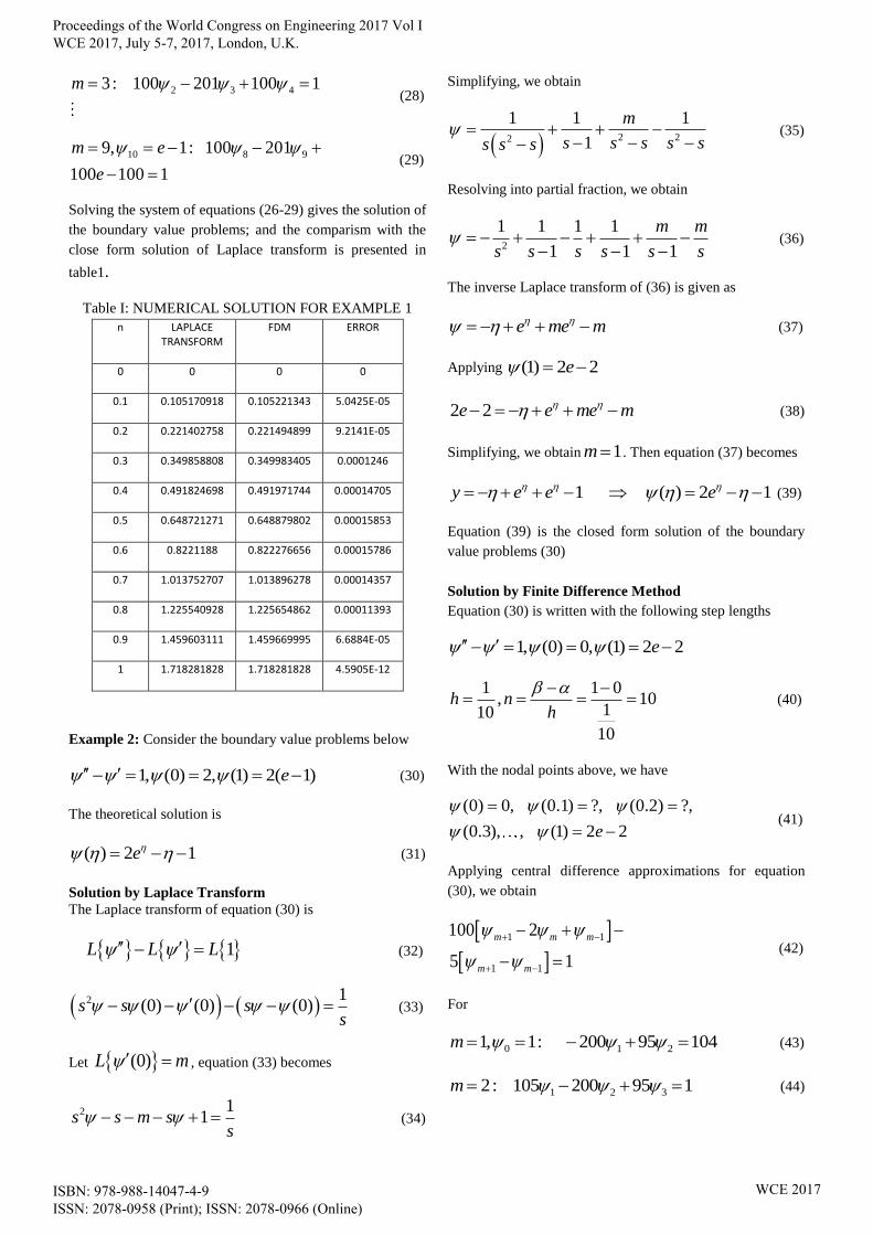
2 3 43: 100 201 100 1m (28)

10 8 99, 1: 100 201

100 100 1

m e

e

(29)

Solving the system of equations (26-29) gives the solution of

the boundary value problems; and the comparism with the

close form solution of Laplace transform is presented in

table1.

Table I: NUMERICAL SOLUTION FOR EXAMPLE 1

n LAPLACE TRANSFORM

FDM ERROR

0 0 0 0

0.1 0.105170918 0.105221343 5.0425E-05

0.2 0.221402758 0.221494899 9.2141E-05

0.3 0.349858808 0.349983405 0.0001246

0.4 0.491824698 0.491971744 0.00014705

0.5 0.648721271 0.648879802 0.00015853

0.6 0.8221188 0.822276656 0.00015786

0.7 1.013752707 1.013896278 0.00014357

0.8 1.225540928 1.225654862 0.00011393

0.9 1.459603111 1.459669995 6.6884E-05

1 1.718281828 1.718281828 4.5905E-12

Example 2: Consider the boundary value problems below

1, (0) 2, (1) 2( 1)e (30)

The theoretical solution is

( ) 2 1e (31)

Solution by Laplace Transform

The Laplace transform of equation (30) is

1L L L (32)

2 1(0) (0) (0)s s s

s (33)

Let (0)L m , equation (33) becomes

2 11s s m s

s (34)

Simplifying, we obtain

2 22

1 1 1

1

m

s s s s ss s s

(35)

Resolving into partial fraction, we obtain

2

1 1 1 1

1 1 1

m m

s s s s s s

(36)

The inverse Laplace transform of (36) is given as

e me m (37)

Applying (1) 2 2e

2 2e e me m (38)

Simplifying, we obtain 1m . Then equation (37) becomes

1 ( ) 2 1y e e e (39)

Equation (39) is the closed form solution of the boundary

value problems (30)

Solution by Finite Difference Method

Equation (30) is written with the following step lengths

1, (0) 0, (1) 2 2e

1 1 0, 10

110

10

h nh

(40)

With the nodal points above, we have

(0) 0, (0.1) ?, (0.2) ?,

(0.3), , (1) 2 2e

(41)

Applying central difference approximations for equation

(30), we obtain

1 1

1 1

100 2

5 1

m m m

m m

(42)

For

0 1 21, 1: 200 95 104m (43)

1 2 32: 105 200 95 1m (44)

Proceedings of the World Congress on Engineering 2017 Vol I WCE 2017, July 5-7, 2017, London, U.K.

ISBN: 978-988-14047-4-9 ISSN: 2078-0958 (Print); ISSN: 2078-0966 (Online)

WCE 2017

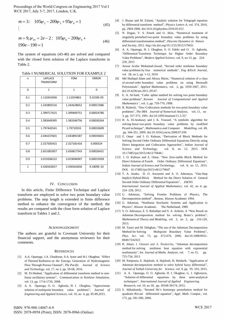
2 3 43: 105 200 95 1m (45)

10 8 99, 2 2 : 105 200

190 190 1

m e

e

(46)

The system of equations (43-46) are solved and compared

with the closed form solution of the Laplace transforms in

Table 2.

Table I NUMERICAL SOLUTION FOR EXAMPLE 2

n LAPLACE TRANSFORM

FDM ERROR

0 1 1 0

0.1 1.110341836 1.11024861 9.3226E-05

0.2 1.242805516 1.242628652 0.00017686

0.3 1.399717615 1.399469751 0.00024786

0.4 1.583649395 1.583346756 0.00030264

0.5 1.797442541 1.79710555 0.00033699

0.6 2.044237601 2.043891587 0.00034601

0.7 2.327505415 2.327181416 0.000324

0.8 2.651081857 2.650817543 0.00026431

0.9 3.019206222 3.019046947 0.00015928

1 3.436563657 3.436563656 9.1809E-10

IV. CONCLUSION

In this article, Finite Difference Technique and Laplace

transform are employed to solve two point boundary value

problems. The step length is extended in finite difference

method to enhance the convergence of the method; the

results are compared with the close form solution of Laplace

transform in Tables 1 and 2.

ACKNOWLEDGMENT

The authors are grateful to Covenant University for their

financial support, and the anonymous reviewers for their

comments.

REFERENCES

[1] A.A. Opanuga, J.A. Gbadeyan, S.A. Iyase and H.I. Okagbue, “Effect

of Thermal Radiation on the Entropy Generation of Hydromagnetic

Flow Through Porous Channel”, The Pacific Journal of Science

and Technology, vol. 17, no 2, pp. 59-68, 2016.

[2] M. El-Shahed, “Application of differential transform method to non-

linear oscillatory systems”, Communication in Nonliear Simulation,

vol. 13, pp. 1714-1720, 2008.

[3] A. A. Opanuga, O. O. Agboola, H. I. Okagbue, “Approximate

solution of multipoint boundary value problems”, Journal of

Engineering and Applied Sciences, vol. 10, no 4, pp. 85-89,2015.

[4] J. Biazar and M. Eslami, “Analytic solution for Telegraph equation

by differential transform method”, Physics Letters A, vol. 374, 2010,

pp. 2904-2906. doi:10.0.16/jphysleta.2010.05.012

[5] N. Dogan, V. S. Erturk and O. Akin, “Numerical treatment of

singularly perturbed two-point boundary value problems by using

differential transformation method”, Discrete Dynamics in Nature

and Society, 2012. http://dx.doi.org/10.1155/2012/579431

[6] A. A. Opanuga, H. I. Okagbue, S. O. Edeki and O. O. Agboola,

“Differential Transform Technique for Higher Order Boundary

Value Problems”, Modern Applied Science, vol. 9, no 13, pp. 224-

230, 2015

[7] Anwar Ja'afar Mohamad-Jawad, “Second order nonlinear boundary

value problems by four numerical methods”, Eng &Tech Journal,

vol. 28, no 2, pp. 1-12, 2010.

[8] Md Shafiqul Islam and Afroza Shirin, “Numerical solution of a class

of second order boundary value problems on using Bernoulli

Polynomials”, Applied Mathematics, vol. 2, pp. 1059-1067, 2011.

doi:10.4236/am.2011.29147.

[9] E. A. Al-Said, “Cubic spline method for solving two point boundary

value problems”, Korean Journal of Computational and Applied

Mathematics”, vol. 5, pp. 759-770, 1998.

[10] B. Bialecki, “Sinc-Collocation methods for two point boundary value

problems”, The IMA Journal of Numerical Analysis, vol. 11, no

3, pp. 357-375, 1991. doi:10.1093/imanum/11.3.357

[11] H. A. El-Arabawy and I. K. Youssef, “A symbolic algorithm for

solving linear two-point boundary value problems by modified

Picard technique”, Mathematica and Computer Modelling, vol. 49,

pp. 344-351, 2009. doi:10.1016/j.mcm.2008.07.030

[12] Z. Omar and J. O. Kuboye, “Derivation of Block Methods for

Solving Second Order Ordinary Differential Equations Directly using

Direct Integration and Collocation Approaches”, Indian Journal of

Science and Technology, vol. 8, no 12, 2015. DOI:

10.17485/ijst/2015/v8i12/70646 |

[13] J. O. Kuboye and Z. Omar, “New Zero-stable Block Method for

Direct Solution of Fourth Order Ordinary Differential Equations”,

Indian Journal of Science and Technology, vol. 8, no 12, 2015.

DOI: 10.17485/ijst/2015/v8i12/70647

[14] T. A. Anake, D. O. Awoyemi and A. O. Adesanya, “One-Step

Implicit Hybrid Block Method for the Direct Solution of General

Second Order Ordinary Differential Equations”, IAENG

International Journal of Applied Mathematics, vol. 42, no 4, pp.

224 -228, 2012.

[15] G. Adomian, “Solving Frontier Problems of Physics, The

Decomposition method” , Boston, Kluwer Academic 1994.

[16] G. Adomian, “Nonlinear Stochastic Systems and Application to

Physics”, Kluwer Academic. The Netherland, 1989.

[17] S. O. Adesanya, E. S. Babadipe and S. A. Arekete, A “New Result on

Adomian Decomposition method for solving Bratu’s problem”,

Mathematical Theory and Modeling, vol. 3, no 2, pp. 116-120,

2013.

[18] M. Tatari and M. Dehghan, “The use of the Adomian Decomposition

Method for Solving Multipoint Boundary Value Problems”,

Phys. Scr. vol. 73, pp. 672-676, 2006. doi:10.1088/0031-

8949/73/6/023

[19] R. Jebari, I. Ghanmi and A. Boukricha, “Adomian decomposition

method for solving nonlinear heat equation with exponential

nonlinearity”, Int. Journal of Maths. Analysis, vol. 7, no 15, pp.

725-734, 2013

[20] M. Paripoura, E. Hajiloub, A. Hajiloub, H. Heidarib, “Application of

Adomian decomposition method to solve hybrid fuzzy differential”,

Journal of Taibah University for Science, vol. 9, pp. 95–103, 2015.

[21] A. A. Opanuga, O. O. Agboola, H. I. Okagbue, G. J. Oghonyon,

“Solution of differential equations by three semi-analytical

techniques”, International Journal of Applied Engineering

Research, vol. 10, no 18, pp. 39168-39174, 2015.

[22] S. Abbasbandy, “Iterated He’s homotopy perturbation method for

quadratic Riccati differential equation”, Appl. Math. Comput., vol.

175, pp. 581-589, 2006.

Proceedings of the World Congress on Engineering 2017 Vol I WCE 2017, July 5-7, 2017, London, U.K.

ISBN: 978-988-14047-4-9 ISSN: 2078-0958 (Print); ISSN: 2078-0966 (Online)

WCE 2017

[23] D. D. Ganji and A. Sadghi, “Application of homotopy-perturbation

and variational iteration methods to nonlinear heat transfer and

porous media equations”, Journal of Computational and Applied

Mathematics, vol. 207, pp. 24-34, 2007.

[24] E.U. Agom and A.M. Badmus, “Correlation of Adomian

decomposition and finite difference methods in solving

nonhomogeneous boundary value problem”, The Pacific Journal

of Science and Technology, vol. 16, no 1, pp. 104-109, 2015

[25] M. L. Dhumal1, S. B. Kiwne, “Finite Difference Method for Laplace

Equation”, International Journal of Statistika and Mathematika, vol.

9, no 1, pp. 11-13, 2014.

[26] S. R. K. Iyengar and R. K. Jain, “Numerical methods”, New Age

International Publishers, 2009, New Delhi, India.

Proceedings of the World Congress on Engineering 2017 Vol I WCE 2017, July 5-7, 2017, London, U.K.

ISBN: 978-988-14047-4-9 ISSN: 2078-0958 (Print); ISSN: 2078-0966 (Online)

WCE 2017