Embed Size (px)
Citation preview
Finite Automata and Algebraicity of Formal Power Series over
Finite Fields
G. Sedanur Albayrak
August 17, 2017
Contents
1 Introduction 2
2 Automatic Sequences 22.1 Repetition in words . . . . . . . . . . . . . . . . . . . . . . . . . . . . . . . . 32.2 Finite Automata . . . . . . . . . . . . . . . . . . . . . . . . . . . . . . . . . 52.3 Automatic Sequences . . . . . . . . . . . . . . . . . . . . . . . . . . . . . . . 62.4 k-automatic Sets . . . . . . . . . . . . . . . . . . . . . . . . . . . . . . . . . 72.5 Multidimensional Automatic Sequences . . . . . . . . . . . . . . . . . . . . 7
3 Cobham’s Theorem 83.1 Morphisms . . . . . . . . . . . . . . . . . . . . . . . . . . . . . . . . . . . . 83.2 Cobham’s Theorem . . . . . . . . . . . . . . . . . . . . . . . . . . . . . . . . 93.3 The k-kernel . . . . . . . . . . . . . . . . . . . . . . . . . . . . . . . . . . . 9
4 Formal Power Series 134.1 Christol’s Theorem . . . . . . . . . . . . . . . . . . . . . . . . . . . . . . . . 134.2 Furstenberg’s Theorem . . . . . . . . . . . . . . . . . . . . . . . . . . . . . . 19
5 Conjecture 265.1 Sparse sets . . . . . . . . . . . . . . . . . . . . . . . . . . . . . . . . . . . . 265.2 Conjecture . . . . . . . . . . . . . . . . . . . . . . . . . . . . . . . . . . . . . 27
Abstract
This project is intended to study the relations of automatic sequences with algebra.To this end, we first look at stringology. We study finite-state automata and then au-tomatic sequences that are produced by finite automata. Then to be able to prove twoimportant results about the relation of automatic sequences and algebraicity of formalpower series over finite fields, we study Cobham’s theorem which is known to be a veryimportant theorem in automata theory. After these two important results, i.e. Chris-tol’s theorem and Furstenberg’s theorem, we present a partial proof of a conjecture ofJason Bell.
The material from sections 2, 3 and 4 of this project comes mostly from [2]. I alsoconsulted [8] and [15] for a specific theorem and a specific example, respectively.
1
1 INTRODUCTION 2
1 Introduction
In this project, we first look at repetition in words in Section 2.1. We introduce the Thue-Morse word which was first given by the Norwegian mathematician Axel Thue in his book[16] in 1912. This sequence is a very interesting sequence since it was rediscovered overthe years by different people including the mathematicians Morse in 1921 [13] and Mahlerin 1927 [10], and by chess master Max Euwe in 1929 (see [7]). The importance of theThue-Morse sequence comes from the fact that it can be used to find an infinite square freeword over a three symbol alphabet. In fact, what Max Euwe showed using the Thue-Morsesequence was that an infinite chess game was possible.
In Section 2.2, we define finite automata which were first studied by Warren S. McCul-loch and Walter H. Pitts in 1943 [11] and finite automata with output which were introducedby George H. Mealy in 1955 [12]. We try to understand the nature of finite automata andhow they work. Then we study sequences that are produced by finite automata. Automaticsequences were first introduced by Alan Cobham in 1972 [6].
In Section 3, we introduce morphisms and then Cobham’s Theorem about uniformmorphisms. We study k-kernels and compute a few examples.
In Section 4, we study Christol’s Theorem which gives an equivalence between an alge-braic property of a formal power series on a finite field and a combinatorial property of thesequence of its coefficients. Christol’s Theorem was first introduced by French mathemati-cian Gilles Christol in 1979 [5]. We also present Christol’s theorem in the multidimensionalsetting which was proved later by Olivier Salon [14]. Then we study Furstenberg’s theorem,which gives an equivalence between algebraic Laurent series over a finite field in n variablesand the diagonal of a rational power series in 2n variables (see [8]).
In Section 5, we try to give a proof of a special case of Jason Bell’s conjecture aboutwhen the Galois group of a Galois extension of Fp(X) adjoined an algebraic series is ap-group.
2 Automatic Sequences
In this section, we will introduce words and specific kind of words. We will look at a specialword called the Thue-Morse word. We will also construct an infinite square free word overa three letter alphabet. Then we will give the definitions of a finite automaton and afinite automaton with output, and we will look at examples of these. We will also give thedefinitions of a k-automatic sequence and k-automatic sets. For the sake of understandingChristol’s Theorem in higher dimensions, we will give the definition of multidimensionalautomatic sequences, too.
To begin with, let Σ denote a nonempty set of symbols. We will call Σ an alphabet.Then a word is a finite or infinite sequence of symbols chosen from Σ. Define Σk :={0, 1, . . . , k − 1}. We will denote the set of all finite words made up of symbols chosenfrom Σ by Σ∗. If n, k ∈ N, then we denote the base-k expansion of n by (n)k. If (n)k =ark
r +ar−1kr−1 + · · ·+a1k+a0, then (n)k = w where w = arar−1 . . . a1a0 for some w ∈ Σ∗.
Similarly, if w is a word such that w = arar−1 . . . a1a0, then we write [w]k = n for somen ∈ N where n = ark
r + ar−1kr−1 + · · ·+ a1k + a0. Also, if w = arar−1 . . . a1a0, we define
wR = a0a1 . . . ar−1ar.

2 AUTOMATIC SEQUENCES 3
2.1 Repetition in words
We begin with the definitions of specific types of words. Then we will prove that thereexists an infinite square free word over a 3-letter alphabet.
Definition 1. A word is said to be square if it is a word of the form xx where x is anyword. A finite or infinite word containing no nonempty square subwords is called squarefree.
Example 1. halhal = (hal)2 is a square, abcabab = abc(ab)2 is not square free.
Definition 2. An overlap is a word of the form cxcxc where x is a (possibly empty) wordand c is a letter. We call a word overlap-free if it contains no overlap.
Example 2. The word soosoos is an overlap with x = oo and c = s.
Here, we introduce an example of a sequence which happens to come out frequently inautomata theory. The Thue-Morse word is given by
tn =
{0 if the number of 1’s in base-2 expansion of n is even,
1 if the number of 1’s in base-2 expansion of n is odd
for n ≥ 1. Then the word t = t0t1t2t3 · · · = 011010011001 . . . is called the Thue-Morseword. Note that we have
t2n = tn (1)
andt2n+1 = 1− tn (2)
for n ≥ 0.
Theorem 1. The Thue-Morse infinite word is overlap-free.
Proof. We follow the proof from Allouche and Shallit [2]. Assume that t contains an overlap.Then t = uaxaxav for some finite words u,x, and an infinite word v. Let m and k denotethe lengths of ax and u, respectively. Then we have
tk+j = tk+j+m for 0 ≤ j ≤ m. (3)
Assume m ≥ 1 is as small as possible. There are two cases:
(i) m is even. Then let m = 2m′ for some integer m′ ≥ 1. There are two cases:
(a) k is even. Then let k = 2k′ for some integer k′ ≥ 1. Then Equation (1) impliesthat tk+2j′ = tk+2j′+m for 0 ≤ j′ ≤ m/2. So, t2k′+2j′ = t2k′+2j′+2m′ for 0 ≤ j′ ≤m′. Since t2n = tn for all n ≥ 0, we get that tk′+j′ = tk′+j′+m′ for 0 ≤ j′ ≤ m′,which contradicts the minimality of m.
(b) k is odd. Then let k = 2k′ + 1 for some integer k′ ≥ 1. Then tk+2j′ = tk+2j′+m
for 0 ≤ j′ ≤ m/2 becomes t2k′+2j′+1 = t2k′+2j′+2m′+1 for 0 ≤ j′ ≤ m′. So,1− tk′+j′ = 1− tk′+j′+m′ , hence, tk′+j′ = tk′+j′+m′ for 0 ≤ j′ ≤ m′. This, again,contradicts the minimality of m.

2 AUTOMATIC SEQUENCES 4
(ii) m is odd. Then we will look at three cases:
(a) m = 1: Then tk = tk+1 = tk+2 by Equation (1). Hence, t2n = t2n+1 forn = dk/2e. This is a contradiction.
(b) m ≥ 5: For n ≥ 1, define bn = (tn + tn+1) mod 2. Now, we have
b4n+2 = (t4n+2 + t4n+1) mod 2 = (t2n+1 + (1− t2n)) mod 2
= ((1− tn) + (1− tn)) mod 2 = (2(1− tn)) mod 2 = 0
and
b2n+1 = (t2n+1 + t2n) mod 2 = ((1− tn) + tn) mod 2
= 1 mod 2 = 1.
Note that we have bk+j = bk+j+m for 1 ≤ j ≤ m. Since m ≥ 5, we can choose1 ≤ j0 ≤ m such that k + j0 ≡ 2 (mod 4). Then k + j0 is of the form 4n + 2.Hence, bk+j0 = 0. On the other hand, since k+j0 is even and m is odd, k+j0+mis odd and bk+j0+m = 1, which is a contradiction.
(c) m = 3: As above, we have bk+j = bk+j+3 for 1 ≤ j ≤ 3. Choose j0 such thatk+j0 ≡ 2 or 3 (mod 4). If k+j0 ≡ 2 (mod 4), then the reasoning in the previouscase applies. If k+ j0 ≡ 3 (mod 4), then k+ j0 is of the form 4n+ 3 = 2(2n) + 1,so bk+j0 = 1. However, bk+j+3 = 0. So, we have a contradiction.
Now, using overlap-freeness of the Thue-Morse word, we construct an infinite squarefree word over a 3-letter alphabet.
Theorem 2. There exists an infinite square free word over the alphabet Σ3 = {0, 1, 2}.
Proof. For n ≥ 1, define cn as the number of 1’s between the nth and (n+ 1)st occurrenceof 0 in the Thue-Morse word t. Set c = c0c1c2 . . . . We will prove that c is square free.
First, observe that c is a word over the alphabet Σ3. If not, then t would contain atleast three consecutive 1’s between two consecutive occurrences of 0, then take a = 1 andx = ε, where ε denotes the empty word, in axaxa which means that t is not overlap-free,which is a contradiction.
Now, assume towards a contradiction that c is not square free. Then it contains asquare, say xx, with x = x1x2 . . . xk, k ≥ 1. But this means t contains a subword of theform
01x101x20 . . . 01xk01x101x20 . . . 01xk0.
Let b = 0, y = 1x101x20 . . . 01xk . Then the Thue-Morse word t contains bybyb which is bydefinition an overlap. This is a contradiction since t is overlap-free.
So there is an infinite square free word over {0, 1, 2} and it is 2102012 . . . (see Example 5).
2 AUTOMATIC SEQUENCES 5
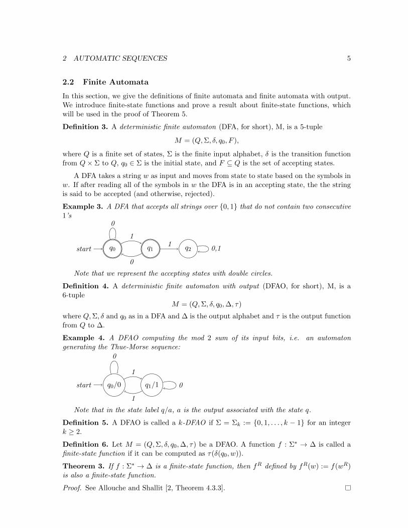
2.2 Finite Automata
In this section, we give the definitions of finite automata and finite automata with output.We introduce finite-state functions and prove a result about finite-state functions, whichwill be used in the proof of Theorem 5.
Definition 3. A deterministic finite automaton (DFA, for short), M, is a 5-tuple
M = (Q,Σ, δ, q0, F ),
where Q is a finite set of states, Σ is the finite input alphabet, δ is the transition functionfrom Q× Σ to Q, q0 ∈ Σ is the initial state, and F ⊆ Q is the set of accepting states.
A DFA takes a string w as input and moves from state to state based on the symbols inw. If after reading all of the symbols in w the DFA is in an accepting state, the the stringis said to be accepted (and otherwise, rejected).
Example 3. A DFA that accepts all strings over {0, 1} that do not contain two consecutive1’s
q0start q1 q2
0
1
0
10,1
Note that we represent the accepting states with double circles.
Definition 4. A deterministic finite automaton with output (DFAO, for short), M, is a6-tuple
M = (Q,Σ, δ, q0,∆, τ)
where Q,Σ, δ and q0 as in a DFA and ∆ is the output alphabet and τ is the output functionfrom Q to ∆.
Example 4. A DFAO computing the mod 2 sum of its input bits, i.e. an automatongenerating the Thue-Morse sequence:
q0/0start q1/1
0
1
0
1
Note that in the state label q/a, a is the output associated with the state q.
Definition 5. A DFAO is called a k-DFAO if Σ = Σk := {0, 1, . . . , k − 1} for an integerk ≥ 2.
Definition 6. Let M = (Q,Σ, δ, q0,∆, τ) be a DFAO. A function f : Σ∗ → ∆ is called afinite-state function if it can be computed as τ(δ(q0, w)).
Theorem 3. If f : Σ∗ → ∆ is a finite-state function, then fR defined by fR(w) := f(wR)is also a finite-state function.
Proof. See Allouche and Shallit [2, Theorem 4.3.3].
2 AUTOMATIC SEQUENCES 6
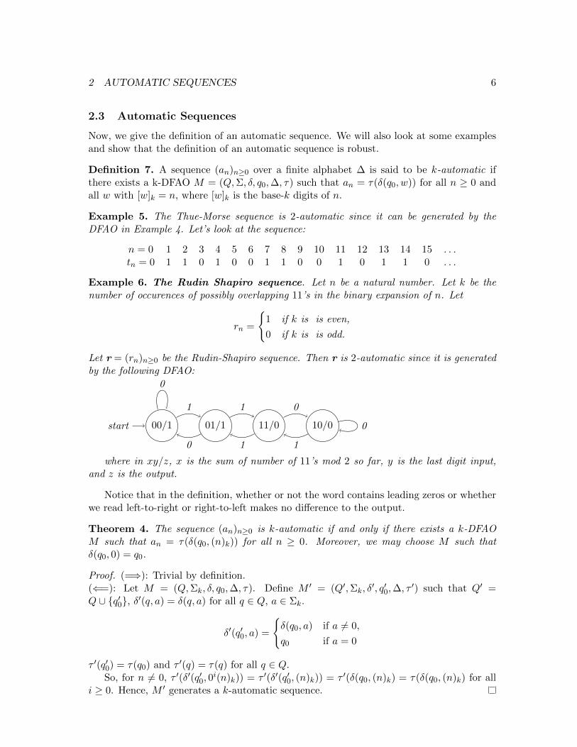
2.3 Automatic Sequences
Now, we give the definition of an automatic sequence. We will also look at some examplesand show that the definition of an automatic sequence is robust.
Definition 7. A sequence (an)n≥0 over a finite alphabet ∆ is said to be k-automatic ifthere exists a k-DFAO M = (Q,Σ, δ, q0,∆, τ) such that an = τ(δ(q0, w)) for all n ≥ 0 andall w with [w]k = n, where [w]k is the base-k digits of n.
Example 5. The Thue-Morse sequence is 2-automatic since it can be generated by theDFAO in Example 4. Let’s look at the sequence:
n = 0 1 2 3 4 5 6 7 8 9 10 11 12 13 14 15 . . .tn = 0 1 1 0 1 0 0 1 1 0 0 1 0 1 1 0 . . .
Example 6. The Rudin Shapiro sequence. Let n be a natural number. Let k be thenumber of occurences of possibly overlapping 11’s in the binary expansion of n. Let
rn =
{1 if k is is even,
0 if k is is odd.
Let r = (rn)n≥0 be the Rudin-Shapiro sequence. Then r is 2-automatic since it is generatedby the following DFAO:
00/1start 01/1 11/0 10/0
0
1 1
0 1
0
1
0
where in xy/z, x is the sum of number of 11’s mod 2 so far, y is the last digit input,and z is the output.
Notice that in the definition, whether or not the word contains leading zeros or whetherwe read left-to-right or right-to-left makes no difference to the output.
Theorem 4. The sequence (an)n≥0 is k-automatic if and only if there exists a k-DFAOM such that an = τ(δ(q0, (n)k)) for all n ≥ 0. Moreover, we may choose M such thatδ(q0, 0) = q0.
Proof. (=⇒): Trivial by definition.(⇐=): Let M = (Q,Σk, δ, q0,∆, τ). Define M ′ = (Q′,Σk, δ
′, q′0,∆, τ′) such that Q′ =
Q ∪ {q′0}, δ′(q, a) = δ(q, a) for all q ∈ Q, a ∈ Σk.
δ′(q′0, a) =
{δ(q0, a) if a 6= 0,
q0 if a = 0
τ ′(q′0) = τ(q0) and τ ′(q) = τ(q) for all q ∈ Q.So, for n 6= 0, τ ′(δ′(q′0, 0
i(n)k)) = τ ′(δ′(q′0, (n)k)) = τ ′(δ(q0, (n)k) = τ(δ(q0, (n)k) for alli ≥ 0. Hence, M ′ generates a k-automatic sequence.

2 AUTOMATIC SEQUENCES 7
Theorem 5. The following are equivalent:
(i) (an)n≥0 is a k-automatic sequence;
(ii) there exists a k-DFAO M = (Q,Σk, δ, q0,∆, τ) such that an = τ(δ(q0, wR)) for all
n ≥ 0 and all w ∈ Σ∗k such that [w]k = n;
(iii) there exists a k-DFAO M ′ = (Q′,Σk, δ′, q′0,∆, τ
′) such that an = τ ′(δ(q0, (n)Rk )) forall n ≥ 0.
Proof. (1) =⇒ (2): Let (an)n≥0 be a k-automatic sequence. By Theorem 3, the functionfR that maps wR to a[w]k is a finite-state function, so there exists a DFAO that computesit.
(2) =⇒ (3): Follows trivially.(3) =⇒ (1): (3) implies that there is a finite-state function g that maps (n)Rk to an.
Hence, by Theorem 3, the function gR is a finite-state function mapping (n)k to an. So, thereexists a DFAO that computes gR. By Theorem 4, we get that (an)n≥0 is k-automatic.
2.4 k-automatic Sets
In this short subsection, we will see the definition of a k-automatic set.
Definition 8. Let S be a subset of nonnegative integers. Then S is called k-automatic ifthe characteristic function of S, i.e.
χS(n) =
{1 if n ∈ S0 if n /∈ S,
defines a k-automatic sequence.
Example 7. Let p be a prime number. S = {1, p, p2, p3, p4, . . . } i.e. powers of p. Then(χS(n))n≥0 is p-automatic.
2.5 Multidimensional Automatic Sequences
We can generalize (n)k and [w]k to pairs of integers and pairs of strings, respectively. Letk,l be integers greater than or equal to 2. Let w be a string over the alphabet Σk × Σl ={0, 1, 2, . . . , k − 1} × {0, 1, 2, . . . , l − 1}. If w = [a1b1][a2b2] . . . [ajbj ], then define [w]k,l =([a1a2 . . . aj ]k, [b1b2 . . . bj ]l). Similarly, if (m)k = a1 . . . ai, (n)l = b1 . . . bj , then (m,n)k,l isdefined as
(m,n)k,l =
{[0, b1] . . . [0, bj−1][a1, bj−i+1] . . . [ai, bj ] if j ≥ i[a1, 0] . . . [ai−j , 0][ai−j+1, b1] . . . [ai, bj ] if i > j.
Definition 9. A two dimensional [k, l]-DFAO is a 6-tuple M = (Q,Σ, δ, q0,∆, τ), where Qis a finite nonempty set of states, Σ = Σk ×Σl, δ : Q×Σ→ Q is the transition function, q0is the initial state, ∆ is the output alphabet and τ : Q → ∆ is the output function. If forall m,n ≥ 0 and for all w ∈ Σ such that [w]k,l = (m,n), we have um,n = τ(δ(q0, w)), thenwe say that M generates the two-dimensional array (ui,j)i,j≥0.

3 COBHAM’S THEOREM 8
Definition 10. A two-dimensional array u is said to be [k, l]-automatic if there exists a[k, l]-DFAO that generates it. If k = l, we will write k-DFAO and k-automatic for brevity’ssake.
Just like k-automatic sequences, we have the following theorem for multidimensionalautomatic sequences.
Theorem 6. The two-dimensional array (ui,j)i,j≥0 is [k, l]-automatic if and only if thereexists a DFAO (Q,Σk × Σl, δ, q0,∆, τ) such that ui,j = τ(δ(q0, (i, j)
Rk,l)) for all i, j ≥ 0.
Proof. The proof is similar to the one dimensional case. See Allouche and Shallit [2, Theo-rem 14.2.1].
We will see the following for 1-dimensional automatic sequences in Section 2.3.
Definition 11. The k-kernel of a two-dimensional array u = (um,n)m,n≥0 is defined asKk,l = {(uka·m+r,la·n+s)m,n≥0 : a ≥ 0, 0 ≤ r < ka, 0 ≤ s < la}.Theorem 7. The two-dimensional array u = (um,n)m,n≥0 is [k, l]-automatic if and only ifthe [k, l]-kernel Kk,l(u) is finite.
Proof. See Allouche and Shallit [2, Theorem 14.2.2].
3 Cobham’s Theorem
In this section, we will study morphisms, uniform morphisms and a theorem about uniformmorphisms due to Cobham. We will also see k-kernels and how a condition on k-kernelsgives automaticity of a sequence.
3.1 Morphisms
We will define morphisms and uniform morphisms, and see a few examples. We will alsoprove a result for uniform morphisms that will be used in the proof of Cobham’s Theorem.Let Σ and ∆ be alphabets.
Definition 12. A morphism is a map h from Σ∗ to ∆∗ satisfying h(xy) = h(x)h(y) for allx, y ∈ Σ∗.
Note that it is sufficient to define h only on Σ since we can extend it to a morphismfrom Σ∗ to ∆∗ uniquely. Note also that the identity h(xy) = h(x)h(y) for all x, y ∈ Σ∗
forces h(ε) = ε.
Example 8. Let Σ = {a, d, y} and ∆ = {a, p}. Set h(d) = ε, h(a) = pa and h(b) = pa.Then h(daddy) = papa.
Definition 13. A morphism h on Σ is called a k-uniform morphism if there exists aconstant k such that |h(a)| = k for all a ∈ Σ. A 1-uniform morphism is called a coding.
Lemma 1. Suppose that w = a0a1a2 . . . is an infinite word with w = φ(w) for somek-uniform morphism φ. Then φ(ai) = akiaki+1aki+2 . . . aki+k−1.
Proof. Since φ is a k-uniform morphism, w = φ(w) implies that φ(a0a1 . . . ai) = a0a1 . . . aki+k−1.Then φ(a0a1 . . . ai−1)φ(ai) = (a0a1 . . . aki−1)(akiaki+1 . . . aki+k−1). Hence,φ(ai) = akiaki+1aki+2 . . . aki+k−1.

3 COBHAM’S THEOREM 9
3.2 Cobham’s Theorem
Now, we can give another description of k-automatic sequences.
Theorem 8 (Cobham [6]). Let k ≥ 2. Then a sequence u = (un)n≥0 is k-automatic if andonly if it is the image, under a coding, of a fixed point of a k-uniform morphism.
Proof. (⇐=): Let τ : ∆ → ∆′ be a coding. Suppose u = τ(w) where w = φ(w) for ak-uniform morphism φ : ∆∗ → ∆∗. Write w = w0w1w2 . . . , wi ∈ ∆ for all i ≥ 0. Letq0 = w0. Define a k-DFAO M = (∆,Σk, δ, q0,∆
′, τ) where δ(q, b) := bth letter of φ(q). Weclaim that wn = δ(q0, (n)k) for all n ≥ 0. We prove it by (strong) induction on n. For n = 0,we have δ(q0, 0) = q0 = w0. Assume wi = δ(q0, (i)k) for all i < n. Let (n)k = n1n2 . . . nt,n = kn′ + nt, 0 ≤ nt < k. Then we have
δ(q0, (n)k) = δ(q0, n1n2 . . . nt)
= δ(δ(q0, n1n2 . . . nt−1), nt)
= δ(δ(q0, (n′)k, nt)
= δ(wn, nt)
= nth letter of φ(wn′)
= wkn′+nt by Lemma 1
= wn.
If u = (un)n≥0, then un = τ(wn) = τ(δ(q0, (n)k). This implies that u is k-automatic byTheorem 4.
(=⇒): Suppose u = (un)n≥0 is k-automatic. Then there exists a k-DFAO (Q,Σk, δ, q,∆, τ)that generates it. By Theorem 4, we can assume that δ(q0, 0) = q0. Define a morphismφ such that φ(q) = δ(q, 0)δ(q, 1) . . . δ(q, k − 1) for all q ∈ Q. Let w = w0w1w2 . . . be thefixed point of φ with w0 = q0. We claim that δ(q0, y) = w[y]k for all y ∈ Σ∗. We provethis by induction on the length of y, |y|. For |y| = 0, we have δ(q0, 0) = q0 = w0. Assumeδ(q0, y) = w[y]k for all y ∈ Σ∗ with |y| < i. Let |y| = i. Write y = xi, where a ∈ Σk,|x| = i− 1. Then we have
δ(q0, y) = δ(q0, xa)
= δ(δ(q0, x), a)
= δ(w[x]k , a) (by the induction hypothesis)
= ath letter in φ(w[x]k) (by definition of φ)
= wk[x]k+a (by Lemma 1)
= w[xa]k
= w[y]k .
So, we get un = τ(δ(q0, (n)k)) = τ(wn). Hence (un)n≥0 is the image (under τ) of the fixedpoint of φ.
3.3 The k-kernel
We define what is a k-kernel of a sequence. Then we give another equivalent description ofautomatic sequences using k-kernels.

3 COBHAM’S THEOREM 10
Definition 14. Let u = (un)n≥0 be an infinite sequence. The k-kernel of u is the set ofsubsequences
Kk(u) = {(uki·n+j)n≥0 : i ≥ 0 and 0 ≤ j < ki}.
Theorem 9. Let k ≥ 2. The infinite sequence u = (un)n≥0 is k-automatic if and only ifKk(u) is finite.
Proof. (=⇒): Assume the sequence u = (un)n≥0 is k-automatic. Then, by Theorem 5,there exists a k-DFAO (Q,Σk, δ, q0,∆, τ) such that un = τ(δ(q0, (n)Rk 0t)) for all t ≥ 0. Letq = δ(q0, w
R), where |w| = i and [w]k = j. For n > 0, we have (ki · n+ j)k = (n)kw. So,
δ(q0, (ki · n+ j)Rk ) = δ(δ(q0, w
R), (n)Rk )
= δ(q, (n)Rk ).
For n = 0, we have (ki · n+ j)k = (j)k and w = 0t(j)k for some t ≥ 0. Then we have
δ(q0, (ki · n+ j)Rk ) = δ(q0, (j)
Rk )
= δ(q0, (j)Rk 0t)
= δ(q0, wR)
= q
= δ(q, (0)Rk )
= δ(q, (n)Rk ).
This shows that the subsequence (uki·n+j)n≥0 is generated by the k-DFAO (Q,Σk, δ, q,∆, τ).Since there are only finitely many choices for q, Kk(u) is finite.
(⇐=): Suppose Kk(u) is finite. Then Σ∗k is partitioned into a finite number of disjointequivalence classes under the equivalence relation
w ≡ x if and only if uk|w|·n+[w]k= uk|x|·n+[x]k
for all n ≥ 0. Now, let [x] denote the equivalence class containing [x] and let Q = {[x] : x ∈Σ∗k}. Define δ([x], a) := [(xa)R] = [ax]. This is well-defined since if [x] = [w] then settingn = km + a gives uk|aw|·m+[aw]k
= uk|ax|·n+[ax]kfor all m ≥ 0. Define τ([w]) = u[w]k . This
is also well-defined because if [x] = [w] then we have u[w]k = u[x]k by choosing n = 0 inuk|w|·n+[w]k
= uk|x|·n+[x]k. Let q0 = [ε]. Then M = (Q,Σk, δ, q0,∆, τ) defines a k-DFAO,
where ∆ = {un : n ≥ 0} is the output alphabet. Observe that
τ(δ(q0, wR)) = τ
([(εwR)R]
)= τ
([(wR)R]
)= τ([w]) = u[w]k
for all w ∈ Σ∗k. Hence u = (un)n≥0 is k-automatic.
Example 9 (2-kernel of the Thue-Morse Sequence). Since we have t2n = tn and t2n+1 =1− tn for the Thue-Morse sequence (tn)n≥0, we get that there are only two subsequences inK2(t). So |K2(t)| = 2. Hence, the 2-kernel of Thue-Morse sequence is finite, as expected.
Example 10 (2-kernel of Rudin-Shapiro Sequence). Let r = (r(n))n≥0 denote the Rudin-Shapiro sequence. We will show that
K2(r) = {(r(n))n≥0, (r(2n+ 1))n≥0, (r(4n+ 3))n≥0, (r(8n+ 3))n≥0}
and hence the Rudin-Shapiro sequence is 2-automatic by Theorem 9.
3 COBHAM’S THEOREM 11
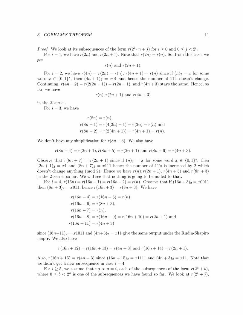
Proof. We look at its subsequences of the form r(2i · n+ j) for i ≥ 0 and 0 ≤ j < 2i.For i = 1, we have r(2n) and r(2n+ 1). Note that r(2n) = r(n). So, from this case, we
getr(n) and r(2n+ 1).
For i = 2, we have r(4n) = r(2n) = r(n), r(4n + 1) = r(n) since if (n)2 = x for someword x ∈ {0, 1}∗, then (4n + 1)2 = x01 and hence the number of 11’s doesn’t change.Continuing, r(4n+ 2) = r(2(2n+ 1)) = r(2n+ 1), and r(4n+ 3) stays the same. Hence, sofar, we have
r(n), r(2n+ 1) and r(4n+ 3)
in the 2-kernel.For i = 3, we have
r(8n) = r(n),
r(8n+ 1) = r(4(2n) + 1) = r(2n) = r(n) and
r(8n+ 2) = r(2(4n+ 1)) = r(4n+ 1) = r(n).
We don’t have any simplification for r(8n+ 3). We also have
r(8n+ 4) = r(2n+ 1), r(8n+ 5) = r(2n+ 1) and r(8n+ 6) = r(4n+ 3).
Observe that r(8n + 7) = r(2n + 1) since if (n)2 = x for some word x ∈ {0, 1}∗, then(2n + 1)2 = x1 and (8n + 7)2 = x111 hence the number of 11’s is increased by 2 whichdoesn’t change anything (mod 2). Hence we have r(n), r(2n+ 1), r(4n+ 3) and r(8n+ 3)in the 2-kernel so far. We will see that nothing is going to be added to that.
For i = 4, r(16n) = r(16n+ 1) = r(16n+ 2) = r(n). Observe that if (16n+ 3)2 = x0011then (8n+ 3)2 = x011, hence r(16n+ 3) = r(8n+ 3). We have
r(16n+ 4) = r(16n+ 5) = r(n),
r(16n+ 6) = r(8n+ 3),
r(16n+ 7) = r(n),
r(16n+ 8) = r(16n+ 9) = r(16n+ 10) = r(2n+ 1) and
r(16n+ 11) = r(4n+ 3)
since (16n+11)2 = x1011 and (4n+3)2 = x11 give the same output under the Rudin-Shapiromap r. We also have
r(16n+ 12) = r(16n+ 13) = r(4n+ 3) and r(16n+ 14) = r(2n+ 1).
Also, r(16n + 15) = r(4n + 3) since (16n + 15)2 = x1111 and (4n + 3)2 = x11. Note thatwe didn’t get a new subsequence in case i = 4.
For i ≥ 5, we assume that up to a = i, each of the subsequences of the form r(2a + b),where 0 ≤ b < 2a is one of the subsequences we have found so far. We look at r(2i + j),
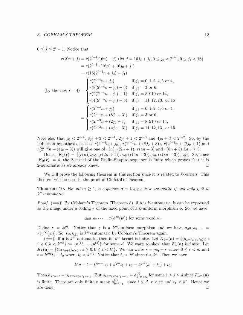
3 COBHAM’S THEOREM 12
0 ≤ j ≤ 2i − 1. Notice that
r(2in+ j) = r(2i−4(16n) + j) (let j = 16j0 + j1, 0 ≤ j0 < 2i−4, 0 ≤ j1 < 16)
= r(2i−4 · (16n) + 16j0 + j1)
= r(16(2i−4n+ j0) + j1)
(by the case i = 4) =
r(2i−4n+ j0) if j1 = 0, 1, 2, 4, 5 or 4,
r(8(2i−4n+ j0) + 3) if j1 = 3 or 6,
r(2(2i−4n+ j0) + 1) if j1 = 8, 910 or 14,
r(4(2i−4n+ j0) + 3) if j1 = 11, 12, 13, or 15
=
r(2i−4n+ j0) if j1 = 0, 1, 2, 4, 5 or 4,
r(2i−1n+ (8j0 + 3)) if j1 = 3 or 6,
r(2i−3n+ (2j0 + 1) if j1 = 8, 910 or 14,
r(2i−2n+ (4j0 + 3)) if j1 = 11, 12, 13, or 15.
Note also that j0 < 2i−4, 8j0 + 3 < 2i−1, 2j0 + 1 < 2i−3 and 4j0 + 3 < 2i−2. So, by theinduction hypothesis, each of r(2i−4n + j0), r(2
i−1n + (8j0 + 3)), r(2i−3n + (2j0 + 1) andr(2i−2n+ (4j0 + 3)) will give one of r(n), r(2n+ 1), r(4n+ 3) and r(8n+ 3) for i ≥ 5.
Hence, K2(r) = {(r(n))n≥0, (r(2n + 1))n≥0, (r(4n + 3))n≥0, (r(8n + 3))n≥0}. So, since|K2(r)| = 4, the 2-kernel of the Rudin-Shapiro sequence is finite which proves that it is2-automatic as we already knew.
We will prove the following theorem in this section since it is related to k-kernels. Thistheorem will be used in the proof of Christol’s Theorem.
Theorem 10. For all m ≥ 1, a sequence a = (ai)i≥0 is k-automatic if and only if it iskm-automatic.
Proof. (=⇒): By Cobham’s Theorem (Theorem 8), if a is k-automatic, it can be expressedas the image under a coding τ of the fixed point of a k-uniform morphism φ. So, we have
a0a1a2 · · · = τ(φ∞(w)) for some word w.
Define γ = φm. Notice that γ is a km-uniform morphism and we have a0a1a2 · · · =τ(γ∞(w)). So, (ai)i≥0 is km-automatic by Cobham’s Theorem again.
(⇐=): If a is km-automatic, then its km-kernel is finite. Let Kkm(a) = {(akmin+b)n≥0 :i ≥ 0, b < kmi} := {a(1), . . . ,a(d)} for some d. We want to show that Kk(a) is finite. LetKk(a) = {(aksn+t)n≥0 : s ≥ 0, 0 ≤ t < ks}. We can write s = mq + r where 0 ≤ r < m andt = kmqt1 + t0 where t0 < kmq. Notice that t1 < kr since t < ks. Then we have
ksn+ t = kqm+rn+ kqmt1 + t0 = kqm(kr + t1) + t0.
Then aksn+t = akqm(kr+t1)+t0 . But akqm(kr+t1)+t0 = a(i)krn+t1
for some 1 ≤ i ≤ d since Kkm(a)
is finite. There are only finitely many a(i)krn+t1
since i ≤ d, r < m and t1 < kr. Hence weare done.

4 FORMAL POWER SERIES 13
4 Formal Power Series
In this section, our goal is to study algebraicity of formal power series when the underlyingfield is finite, and their relations with finite automata.We begin with stating some well-known results.
Remark 1. If a field F is of characteristic p, then (a + b)p = ap + bp for all a, b ∈ F .Let K = GF (q) where q = pn, paprime. Let A(X) ∈ K[[X]]. Then A(Xq) = A(X)q. LetF (X) =
∑n≥n0
anXn ∈ K((X)) be a formal Laurent series. We say that F is algebraic
over K(X), if there exist d ≥ 1 and polynomials A0(X), A1(X), . . . , Ad(X) with coefficientsin K which are not all zero such that
A0 +A1F + · · ·+AdFd = 0.
4.1 Christol’s Theorem
A basic result in the study of the relation between formal power series and finite automatais Christol’s theorem, which gives an equivalence between an algebraic property of a formalpower series on a finite field and a combinatorial property of the sequence of its coefficients.Let us first look at some examples before giving the formal statement of Christol’s Theorem.Then we will introduce necessary tools to be able to prove Christol’s Theorem.
Example 11. Let p be a prime number. Let f(X) ∈ Fp[[X]] such that f(X) = X + Xp +
Xp2 +Xp3 + · · · =∑
i≥0Xpi. We will see that f(X) is algebraic over Fp(X) since
f(Xp) =∑i≥0
Xpi+1= Xp +Xp2 +Xp3 +Xp4 + · · ·
= f(X)−X.
Note that over Fp, we have f(Xp) = f(X)p. So we get f(X)p− f(X) +X = 0 which showsthat f(X) is algebraic over Fp(X).
In fact, this provides a proof to Example 7, assuming Christol’s Theorem.
Example 12. Let T (X) =∑
n≥0 tnXn, where (tn)n≥0 is the Thue-Morse sequence. We
have T (X) is algebraic over F2(X).
Proof.
T (X) =∑
tnXn =
∑t2nX
2n +∑
t2n+1X2n+1
=∑
tnX2n +
∑(1− tn)X2n+1 by Equation (1) and Equation (2)
=∑
tnX2n +
∑(1 + tn)X2n+1 since we are in F2[[X]]
=∑
tnX2n +X ·
∑(1 + tn)X2n
=∑
tn(X2)n +X ·∑
tn(X2)n +X∑
(X2)n
4 FORMAL POWER SERIES 14
= T (X2) +X · T (X2) +X1
1−X2
= T (X)2 +X · T (X)2 +X1
1 +X2since we are in F2[[X]]
= (1 +X) · T (X)2 +X1
(1 +X)2since we are in F2[[X]].
So
T (X) = (1 +X) · T (X)2 +X1
(1 +X)2
(1 +X)2T (X) = (1 +X)3T (X)2 +X.
Hence we get(1 +X)3T (X)2 + (1 +X)2T (X) +X = 0 (4)
which shows that T (X) is algebraic over F2(X).
In fact, we can generalize the previous example for any prime p.
Example 13. Let sp(n) denote the sequence of sum of digits of the base-p expansion of n.Let tp(n) = sp(n)(mod p) and let Tp(X) =
∑n≥0 tp(n)Xn. Note that we can write it as
Tp(X) =∑
0≤a<p
∑n≥0
tp(pn+ a)Xpn+a
=∑
0≤a<p
∑n≥0
(tp(n) + a)Xpn+a
=∑
0≤a<pXa∑n≥0
tp(n)(Xp)n +∑
0≤a<p
∑n≥0
aXpn+a
=∑
0≤a<pXaTp(X
p) +
∑0≤a<p
aXa∑n≥0
(Xn)p
=∑
0≤a<pXaTp(X)p +
∑0≤a<p
aXa
∑n≥0
Xn
p= Tp(X)p
∑0≤a<p
Xa +1
(1−X)p
∑0≤a<p
aXa
= Tp(X)p1−Xp
1−X+
1
(1−X)p
∑0≤a<p
aXa
= Tp(X)p1−Xp
1−X+
1
(1−X)pX(1−Xp)
(1−X)2
= Tp(X)p1−Xp
1−X+
X
(1−X)2.

4 FORMAL POWER SERIES 15
So
(1−X)p+1Tp(X)p − (1−X)2Tp(X) +X = 0.
Hence Tp(X) is algebraic over Fp(X).
We see that these examples are not coincidences and Christol proves a general resultthat explains them.
Theorem 11. Let ∆ be a nonempty finite set, let a = (ai)i≥0 be a sequence that takesvalues in ∆, and let p be a prime number. Then a is p-automatic if and only if there existan integer n ≥ 1 and an injective map β : ∆ → Fq such that
∑i≥1 β(ai)X
i ∈ Fq[[X]] isalgebraic over Fq(X), where q = pn.
Before we prove Christol’s Theorem, we introduce the Cartier operators and look atsome of their properties.
Definition 15. For 0 ≤ r < q, a linear transformation Λr : Fq[[X]]→ Fq[[X]] such that
Λr
∑i≥0
aiXi
=∑i≥0
aqi+rXi
is called the rth-Cartier operator.
Lemma 2. Let A,B ∈ Fq[[X]]. Then the rth-Cartier operator has the following properties:
(i) A(X) =∑
i≥0 aiXi =
∑0≤r<qX
rΛr(A(X))q;
(ii) Λr(AqB) = AΛr(B).
Proof. (i)
A(X) =∑i≥0
aiXi =
∑0≤r<q
∑i≥0
aqi+rXqi+r
=∑
0≤r<qXr∑i≥0
aqi+rXiq
=∑
0≤r<qXr
∑i≥0
aqi+rXi
q
=∑
0≤r<qXr (Λr(A(X)))q .

4 FORMAL POWER SERIES 16
(ii) Let B(X) =∑
k≥0 bkXk, then we have
Λr(AqB) = Λr
∑i≥0
aiXi
q∑k≥0
bkXk
= Λr
∑i≥0
aiXqi
∑k≥0
bkXk
= Λr
∑j≥0
Xj
∑i,k≥0,qi+k=j
aibk
=∑j≥0
Xj
∑i,k≥0,qi+k=qj+r
aibk
=∑j≥0
Xj
∑0≤i≤j
aibq(j−i)+r
=∑i≥0
aiXi
∑j≥i
bq(j−i)+rXj−i
=
∑i≥0
aiXi
∑k≥0
bqk+rXk
= A · Λr(B).
We need two more lemmas to use in the proof of Christol’s Theorem.
Lemma 3. Let A(X) ∈ Fq[[X]], q = pn. Then A is algebraic over Fq(X) if and only ifthere exists polynomials B0(X), B1(X), B2(X), . . . , Bt(X), not all zero, such that
B0A+B1Aq +B2A
q2 + · · ·+BtAqt = 0.
Furthermore, we can assume that B0 6= 0.
Proof. (=⇒): Suppose A(X) is algebraic over Fq(X). Let t be the degree of its minimal
polynomial. Then A,Aq, Aq2, . . . , Aq
tcannot be linearly independent over Fq(X) since there
are t+ 1 of them. Hence there exists a nontrivial linear relation
B0A+B1Aq + · · ·+BtA
qt = 0
where B0, B1, . . . , Bt ∈ Fq[X].(⇐=): Trivial.Now it remains to show that we can in fact assume B0 6= 0. We pick a nontrivial relation
of the formB0A+B1A
q +B2Aq2 + · · ·+BtA
qt = 0
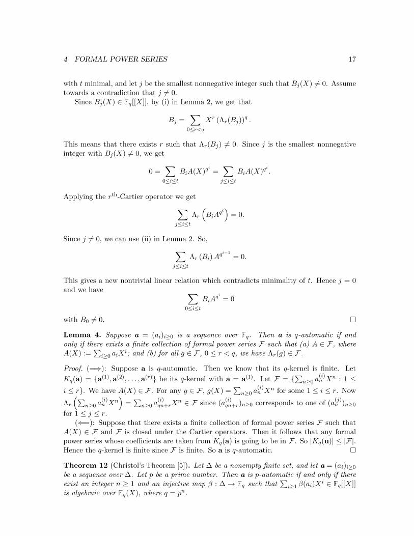
4 FORMAL POWER SERIES 17
with t minimal, and let j be the smallest nonnegative integer such that Bj(X) 6= 0. Assumetowards a contradiction that j 6= 0.
Since Bj(X) ∈ Fq[[X]], by (i) in Lemma 2, we get that
Bj =∑
0≤r<qXr (Λr(Bj))
q .
This means that there exists r such that Λr(Bj) 6= 0. Since j is the smallest nonnegativeinteger with Bj(X) 6= 0, we get
0 =∑0≤i≤t
BiA(X)qi
=∑j≤i≤t
BiA(X)qi.
Applying the rth-Cartier operator we get∑j≤i≤t
Λr
(BiA
qi)
= 0.
Since j 6= 0, we can use (ii) in Lemma 2. So,∑j≤i≤t
Λr (Bi)Aqi−1
= 0.
This gives a new nontrivial linear relation which contradicts minimality of t. Hence j = 0and we have ∑
0≤i≤tBiA
qi = 0
with B0 6= 0.
Lemma 4. Suppose a = (ai)i≥0 is a sequence over Fq. Then a is q-automatic if andonly if there exists a finite collection of formal power series F such that (a) A ∈ F , whereA(X) :=
∑i≥0 aiX
i; and (b) for all g ∈ F , 0 ≤ r < q, we have Λr(g) ∈ F .
Proof. (=⇒): Suppose a is q-automatic. Then we know that its q-kernel is finite. Let
Kq(a) = {a(1),a(2), . . . ,a(r)} be its q-kernel with a = a(1). Let F = {∑
n≥0 a(i)n Xn : 1 ≤
i ≤ r}. We have A(X) ∈ F . For any g ∈ F , g(X) =∑
n≥0 a(i)n Xn for some 1 ≤ i ≤ r. Now
Λr
(∑n≥0 a
(i)n Xn
)=∑
n≥0 a(i)qn+rX
n ∈ F since (a(i)qn+r)n≥0 corresponds to one of (a
(j)n )n≥0
for 1 ≤ j ≤ r.(⇐=): Suppose that there exists a finite collection of formal power series F such that
A(X) ∈ F and F is closed under the Cartier operators. Then it follows that any formalpower series whose coefficients are taken from Kq(a) is going to be in F . So |Kq(u)| ≤ |F|.Hence the q-kernel is finite since F is finite. So a is q-automatic.
Theorem 12 (Christol’s Theorem [5]). Let ∆ be a nonempty finite set, and let a = (ai)i≥0be a sequence over ∆. Let p be a prime number. Then a is p-automatic if and only if thereexist an integer n ≥ 1 and an injective map β : ∆ → Fq such that
∑i≥1 β(ai)X
i ∈ Fq[[X]]is algebraic over Fq(X), where q = pn.
4 FORMAL POWER SERIES 18
Proof of Christol’s Theorem. We can choose n sufficiently large so that |∆| ≤ pn, and aninjective map β : ∆→ Fpn . Hence, we may assume without loss of generality that ∆ ⊆ Fpn .
(=⇒): We will show that∑aiX
i is algebraic over Fpn(X). By Theorem 10, (ai)i≥0 ispn automatic since it is p-automatic. Then its q-kernel, Kq(a), is finite by Theorem 9. So,let Kq(a) = {a(1),a(2), . . . ,a(d)} for some integer d, where a(1) = a. Define
Aj(X) =∑n≥0
a(j)n Xn
for 1 ≤ j ≤ d. Rewriting,
Aj(X) =∑
0≤r≤q−1
∑m≥0
a(j)qm+rX
qm+r =∑
0≤r≤q−1Xr
∑m≥0
a(j)qm+rX
qm.
Since (a(j)qm+r)m≥0 is one of a(i) for 1 ≤ i ≤ d, Aj(X) is an Fq[X]-linear combination of
the power series Ai(Xq). In other words, Aj(X) is in Fq(X)-vector space generated by the
series Ai(Xq). So for all j, 1 ≤ j ≤ d, we have
Aj(X) ∈ 〈A1(Xq), . . . , Ad(X
q)〉.
This implies for all j, 1 ≤ j ≤ d, Aj(Xq) ∈ 〈A1(X
q2), . . . , Ad(Xq2)〉. So,
Aj(X), Aj(Xq) ∈ 〈A1(X
q2), . . . , Ad(Xq2)〉.
Also, Aj(Xq2) ∈ 〈A1(X
q3), . . . , Ad(Xq3)〉 for all j, 1 ≤ j ≤ d. So,
Aj(X), Aj(Xq), Aj(X
q2) ∈ 〈A1(Xq3), . . . , Ad(X
q3)〉.
Continuing in this manner, we get
Aj(X), Aj(Xq), Aj(X
q2), . . . , Aj(Xqd) ∈ 〈A1(X
qd+1), . . . , Ad(X
qd+1)〉.
Notice that the dimension of 〈A1(Xqd+1
), . . . , Ad(Xqd+1
)〉 over Fq(X) as a vector space is
at most the number of generators which is d. So Aj(X), Aj(Xq), Aj(X
q2) . . . , Aj(Xqd) are
linearly dependent over Fpn(X). So, by Lemma 3, Aj(X) is algebraic over Fpn for all1 ≤ j ≤ d. In particular, for j = 1, A1(X) = A(X) =
∑i≥0 aiX
i is algebraic over Fpn(X),which proves our assertion.
(⇐=): Assume that A(X) =∑
i≥0 aiXi is algebraic over Fq(X). Then by Lemma 3
there exist B0(X), B1(X), . . . , Bt(X) such that
B0(X)A(X) +B1A(X)q + · · ·+BtA(X)qt
= 0 (5)
with B0(X) 6= 0. Put G = A(X)B0(X) . Dividing both sides by B0(X)2 in Equation (5), we get
A(X)
B0(X)+
B1(X)
B0(X)2A(X)q + · · ·+ Bt(X)
B0(X)2A(X)q
t= 0.
Now, multiply and divide ith term by B0(X)qi
for 2 ≤ i ≤ t. So, we get
A(X)
B0(X)+
B1(X)B0(X)q
B0(X)2B0(X)qA(X)q + · · ·+ Bt(X)B0(X)q
t
B0(X)2B0(X)qtA(X)q
t= 0.
4 FORMAL POWER SERIES 19
Now, substituting G, we get
G+B1(X)B0(X)q−2Gq + · · ·+Bt(X)B0(X)qt−2Gq
t= 0.
From this, we get G = −∑t
i=1Bi(X)B0(X)qi−2Gq
i. Let Ci = −Bi(X)B0(X)q
i−2 for 1 ≤i ≤ t. Then G =
∑ti=1Ci(X)Gq
i. Now, let N = max (degB0,maxi degCi). Let H = {H ∈
Fq[[X]] : H =∑
0≤i≤tDiGqi , Di ∈ Fq[X], degDi ≤ N}. Observe that H is a finite set since
degDi ≤ N for each i. Also, A = B0G ∈ H since degB0 ≤ N by definition of N . If we canshow that H is mapped into itself under Λr, then we can use Lemma 4 and conclude that(ai)i≥0 is q-automatic. Take any H ∈ H, look at:
Λr(H) = Λr
D0G+∑1≤i≤t
DiGqi
= Λr
∑1≤i≤t
D0CiGqi +
∑1≤i≤t
DiGqi
= Λr
∑1≤i≤t
(D0Ci +Di)Gqi
=∑1≤i≤t
Λr
((D0Ci +Di)G
qi)
(linearity)
=∑1≤i≤t
Λr(D0Ci +Di)Gqi−1 by (ii) in Lemma 2.
Now, observe that degD0 ≤ N and degDi ≤ N for all 1 ≤ i ≤ t by definition of H. Also,degCi ≤ N for all 1 ≤ i ≤ t by definition of N . So, we get deg (D0Ci +Di) ≤ 2N . Hence,
deg (Λr(D0Ci +Di)) ≤2N
q≤ N
since q ≥ 2. Therefore, a is q-automatic. By Theorem 10, a is p-automatic.
We can generalize Christol’s Theorem to the multidimensional case.
Theorem 13 (Christol’s Theorem in higher dimension). Let p be a prime number. Thesequence (um,n)m,n≥0 over ∆ is [p, p]-automatic, or in short p-automatic, if and only if thereexist an integer n ≥ 1 and an injective map b : ∆→ Fpn such that
∑m≥0,n≥0 b(um,n)XmY n
is algebraic over Fpn [X,Y ].
Proof. The proof is a straightforward extension of Theorem 12 to the higher dimensionalsetting.
4.2 Furstenberg’s Theorem
Furstenberg’s Theorem gives us a way to get an algebraic formal power series using rationalpower series in higher dimension.
4 FORMAL POWER SERIES 20
Definition 16. LetF (X,Y ) =
∑m≥m0,n≥n0
am,nXmY n,
where m0, n0 ∈ Z, be a formal Laurent series in two variables. The diagonal DF is theformal Laurent series in one variable defined by
DF (t) = D
∑m≥m0,n≥n0
am,nXmY n
:=∑
k≥max {m0,n0}
ak,ktk.
Example 14. Let F (X,Y ) = 11−X−Y . We have
1
1−X − Y=∑n≥0
(X + Y )n =∑n≥0
n∑k=0
(n
k
)XkY n−k.
Then the diagonal terms occur when k = n− k. So
DF (t) =∑k≥0
(2k
k
)tk = 1 + 2t+ 6t2 + 20t3 + · · · =: f(t).
Observe that
(1− 4t)−1/2 = 1 +
(−1/2
1
)(−4t) +
(−1/2
2
)(−4t)2 +
(−1/2
3
)(−4t)3+
· · ·+(−1/2
n
)(−4t)n + · · ·
= 1 + 2t+ 6t2 + 20t3 + · · ·= f(t) (or see [15, Exercise 4a]).
So f(t) = (1− 4t)−1/2 implies (1− 4t)f(t)2 − 1 = 0. Hence f(t) = DF (X,Y ) is algebraic.
Example 15. Consider the rational function in two variables
R(X,Y ) =2Y
2− Y 2(1−XY )2 − X(1−XY )3
over F3(X,Y ). Note that we have
X
(1−XY )3= X
∑i≥0
(XY )3i
over F3(X,Y ). We will compute the diagonal but we will require a theorem below to finishthe computation.
4 FORMAL POWER SERIES 21
R(X,Y ) =2Y
2− Y 2(1−XY )2 −X∑
i≥0(XY )3i
=Y
1− Y 2
2 (1−XY )2 − X2
∑i≥0(XY )3i
= Y∑j≥0
2−j
Y 2(1−XY )2 +X∑i≥0
(XY )3i
j
=∑
j≥0,k≥02−j(j
k
)Y 2k+1(1−XY )2kXj−k
∑i≥0
(XY )3i
j−k
:=∑m,n≥0
am,nXmY n.
Let us calculate the diagonal DR(t) =∑
n≥0 an,ntn. Notice that the only indices that
can give equal exponents for X and Y is when j − k = 2k + 1. So, substitute j = 3k + 1.Then we have
DR(t) =∑k≥0
2−(3k+1)
(3k + 1
k
)t2k+1(1− t)2k
∑i≥0
t3i
2k+1
=∑k≥0
2−(3k+1)
(3k + 1
k
)t2k+1(1− t)−4k−3.
We can write DR(t) as follows:
DR(t) =∑k≥0
2−(9k+1)
(9k + 1
3k
)t6k+1(1− t)−12k−3
+∑k≥0
2−(9k+4)
(9k + 4
3k + 1
)t6k+3(1− t)−12k−7
+∑k≥0
2−(9k+7)
(9k + 7
3k + 2
)t6k+5(1− t)−12k−11.
(6)
Now, to be able to simplify this equation, we look at the following theorem originallydue to Edouard Lucas (see [9]).
Theorem 14. Let p be a prime number. Let n and j be natural numbers. Without loss ofgenerality, assume j ≤ n. Let (n)p = ad . . . a0 and (j)p = je . . . j0 for some e, d ≥ 1 be thebase-p expansions of n and j, respectively. If e < d, put jd = jd−1 = · · · = je+1 = 0 so that(j)p = jd . . . j0. Then
(nj
)≡(adjd
)· · ·(a0j0
)mod p.
Proof. Notice we have |(n)p| = |(j)p|. We use induction on |(n)p|. If |(n0)| = 1. Thenn = n0, j = j0, 0 ≤ n0, j0 ≤ p − 1, and the result follows trivially. Assume that the
4 FORMAL POWER SERIES 22
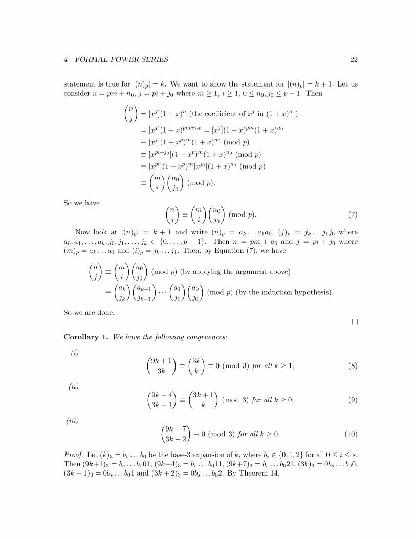
statement is true for |(n)p| = k. We want to show the statement for |(n)p| = k + 1. Let usconsider n = pm+ n0, j = pi+ j0 where m ≥ 1, i ≥ 1, 0 ≤ n0, j0 ≤ p− 1. Then(
n
j
)= [xj ](1 + x)n (the coefficient of xj in (1 + x)n )
= [xj ](1 + x)pm+n0 = [xj ](1 + x)pm(1 + x)n0
≡ [xj ](1 + xp)m(1 + x)n0 (mod p)
≡ [xpi+j0 ](1 + xp)m(1 + x)n0 (mod p)
≡ [xpi](1 + xp)m[xj0 ](1 + x)n0 (mod p)
≡(m
i
)(n0j0
)(mod p).
So we have (n
j
)≡(m
i
)(n0j0
)(mod p). (7)
Now look at |(n)p| = k + 1 and write (n)p = ak . . . a1a0, (j)p = jk . . . j1j0 wherea0, a1, . . . , ak, j0, j1, . . . , jk ∈ {0, . . . , p − 1}. Then n = pm + a0 and j = pi + j0 where(m)p = ak . . . a1 and (i)p = jk . . . j1. Then, by Equation (7), we have(
n
j
)≡(m
i
)(a0j0
)(mod p) (by applying the argument above)
≡(akjk
)(ak−1jk−1
)· · ·(a1j1
)(a0j0
)(mod p) (by the induction hypothesis).
So we are done.
Corollary 1. We have the following congruences:
(i) (9k + 1
3k
)≡(
3k
k
)≡ 0 (mod 3) for all k ≥ 1; (8)
(ii) (9k + 4
3k + 1
)≡(
3k + 1
k
)(mod 3) for all k ≥ 0; (9)
(iii) (9k + 7
3k + 2
)≡ 0 (mod 3) for all k ≥ 0. (10)
Proof. Let (k)3 = bs . . . b0 be the base-3 expansion of k, where bi ∈ {0, 1, 2} for all 0 ≤ i ≤ s.Then (9k+1)3 = bs . . . b001, (9k+4)3 = bs . . . b011, (9k+7)3 = bs . . . b021, (3k)3 = 0bs . . . b00,(3k + 1)3 = 0bs . . . b01 and (3k + 2)3 = 0bs . . . b02. By Theorem 14,

4 FORMAL POWER SERIES 23
(i) (9k + 1
3k
)≡(bs . . . b00
0bs . . . b0
)(1
0
)(mod 3) ≡
(3k
k
)(mod 3).
Since k ≥ 1, there exists i with bi 6= 0. Let i0 be the smallest index such thatbi0 ∈ {1, 2}. Then bi0−1 = · · · = b0 = 0. Then we have(
3k
k
)≡(bs0
)· · ·(bi0−1bi0
)· · ·(
0
b0
)(mod 3)
≡(bs0
)· · ·(
0
bi0
)· · ·(
0
b0
)(mod 3)
≡ 0 (mod 3) since both
(0
1
)and
(0
2
)are 0.
(ii) (9k + 4
3k + 1
)≡(bs . . . b01
0bs . . . b0
)(1
1
)(mod 3) ≡
(3k + 1
k
)(mod 3).
(iii) (9k + 7
3k + 2
)≡(bs . . . b02
0bs . . . b0
)(1
2
)(mod 3) ≡ 0 (mod 3).
Returning to Example 15, over F3(X,Y ), Equation (6) becomes
DR(t) =∑k≥0
2−(9k+1)
(9k + 1
3k
)t6k+1(1− t)−12k−3
+∑k≥0
2−(9k+4)
(9k + 4
3k + 1
)t6k+3(1− t)−12k−7
+∑k≥0
2−(9k+7)
(9k + 7
3k + 2
)t6k+5(1− t)−12k−11,
which by Corollary 1 simplifies to
1
2t(1− t)−3 +
∑k≥0
1
2
(2−(3k+1)
)3(3k + 1
k
)(t2k+1)3
((1− t)−4k−3
)3(1− t)2
=t
2(1− t)−3 +
(1− t)2
2(DR)3(t).
So, multiplying both sides by 2(1− t)3, we get
(1− t)5(DR)3(t) + (1− t)3(DR)(t) + t = 0 (11)
Thus (DR)(t) is algebraic over F3(t).
4 FORMAL POWER SERIES 24
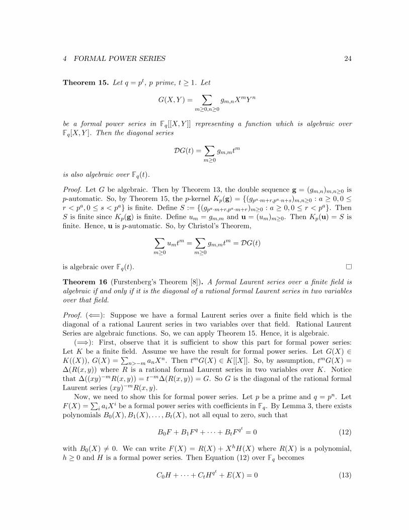
Theorem 15. Let q = pt, p prime, t ≥ 1. Let
G(X,Y ) =∑
m≥0,n≥0gm,nX
mY n
be a formal power series in Fq[[X,Y ]] representing a function which is algebraic overFq[X,Y ]. Then the diagonal series
DG(t) =∑m≥0
gm,mtm
is also algebraic over Fq(t).
Proof. Let G be algebraic. Then by Theorem 13, the double sequence g = (gm,n)m,n≥0 isp-automatic. So, by Theorem 15, the p-kernel Kp(g) = {(gpa·m+r,pa·n+s)m,n≥0 : a ≥ 0, 0 ≤r < pa, 0 ≤ s < pa} is finite. Define S := {(gpa·m+r,pa·m+r)m≥0 : a ≥ 0, 0 ≤ r < pa}. ThenS is finite since Kp(g) is finite. Define um = gm,m and u = (um)m≥0. Then Kp(u) = S isfinite. Hence, u is p-automatic. So, by Christol’s Theorem,∑
m≥0umt
m =∑m≥0
gm,mtm = DG(t)
is algebraic over Fq(t).
Theorem 16 (Furstenberg’s Theorem [8]). A formal Laurent series over a finite field isalgebraic if and only if it is the diagonal of a rational formal Laurent series in two variablesover that field.
Proof. (⇐=): Suppose we have a formal Laurent series over a finite field which is thediagonal of a rational Laurent series in two variables over that field. Rational LaurentSeries are algebraic functions. So, we can apply Theorem 15. Hence, it is algebraic.
(=⇒): First, observe that it is sufficient to show this part for formal power series:Let K be a finite field. Assume we have the result for formal power series. Let G(X) ∈K((X)), G(X) =
∑n>−m anX
n. Then tmG(X) ∈ K[[X]]. So, by assumption, tmG(X) =∆(R(x, y)) where R is a rational formal Laurent series in two variables over K. Noticethat ∆((xy)−mR(x, y)) = t−m∆(R(x, y)) = G. So G is the diagonal of the rational formalLaurent series (xy)−mR(x, y).
Now, we need to show this for formal power series. Let p be a prime and q = pn. LetF (X) =
∑i aiX
i be a formal power series with coefficients in Fq. By Lemma 3, there existspolynomials B0(X), B1(X), . . . , Bt(X), not all equal to zero, such that
B0F +B1Fq + · · ·+BtF
qt = 0 (12)
with B0(X) 6= 0. We can write F (X) = R(X) + XhH(X) where R(X) is a polynomial,h ≥ 0 and H is a formal power series. Then Equation (12) over Fq becomes
C0H + · · ·+ CtHqt + E(X) = 0 (13)

4 FORMAL POWER SERIES 25
where Ci = BiXqih and E(X) = B0R+ · · ·+BtRq
t. Now, we show that in Equation (13) we
can assume H(0) = 0 and C0(0) 6= 0. First, if H(0) 6= 0, then put H(X) = H(X)−H(0).Then H(0) = 0 and Equation (13) becomes
C0H + C1Hq + · · ·+ CtH
qt + E(X) = 0
where E(X) = C0H(0) + C1H(0)q + · · · + CtH(0)qt
+ E(X) and we can write F (X) =(R(X) +H(0)Xh
)+XhH where R(X)+H(0)Xh is a polynomial. So we are done. Suppose
towards a contradiction that C0(0) = 0. Then since Ci are polynomials there exists at leastone integer, say j, such that Xj divides C0(X) and Xj+1 does not divide C0(X). Let rbe the smallest integer among all such j’s. Let H(X) =
∑i≥0 λiX
i = λ0 +XK(X) whereK(X) is a power series. Then Equation (13) becomes
C0XK + C1XqKq + · · ·+ CtX
qtKqt + E = 0 (14)
where E = E + λ0C0 + · · ·+ λqt
0 Ct and F (X) = R(X) + λ0Xh +Xh+1K.
Let s = min (r + 1, q). Observe that Xs divides CiXqiKqi for all 0 ≤ i ≤ t. Hence, by
Equation (14), Xs divides E. If we divide Equation (14) by Xs, the type of the equationdoesn’t change and we get that Xr−s+1 divides the first coefficient whereas Xr−s+2 doesnot. Suppose r 6= 0. Then 0 ≤ r− s+ 1 < r. So, we get a contradiction. Hence r = 0 whichmeans X does not divide C0. Hence C0(0) 6= 0.
Now define the following polynomial
P (X,Y ) = C0(X)Y + C1(X)Y q + · · ·+ Ct(X)Y qt + E(X). (15)
Observe that P (X,H(X)) = 0. We can consider P as a polynomial in Fq((X))[Y ]. Wecan then write P (X,Y ) = (Y −H(X))Q(X,Y ) where Q(X,Y ) is a polynomial in Y withcoefficients in Fq((X)). Notice that ∂P
∂Y (0, 0) = C0(0) and by what we have shown abovethat is nonzero. If we take the partial derivative of both sides in Equation (15), we get∂P∂Y (0, 0) = Q(0, 0) − H(0)∂Q∂Y (0, 0) = Q(0, 0). So, Q(0, 0) 6= 0. Now, taking logarithms ofboth sides in Equation (15) and then taking partial derivatives, we get
1
P
∂P
∂Y(X,Y ) =
1
Y −H(X)+
1
Q
∂Q
∂Y(X,Y ). (16)
Since Q(0, 0) 6= 0, 1Q∂Q∂Y (X,Y ) can be expanded as a formal Laurent series in two vari-
ables. Now, multiplying both sides in Equation (16) by Y 2, replacing X by XY and takingdiagonals, we have
D(
Y 2
P (XY, Y )
∂P
∂Y(XY, Y )
)= D
(Y 2
Y −H(XY )
)+D
(Y 2
Q(XY, Y )
∂Q
∂Y(XY, Y )
). (17)
Notice that the second term on the left-hand side of Equation (17) is the diagonal of a

5 CONJECTURE 26
series in XY and Y multiplied by Y 2, so it is 0. Also,
D(
Y 2
Y −H(XY )
)= D
(Y
1−H(XY )/Y
)
= D
Y ∑i≥0
(H(XY )/Y )i
= D
∑i≥0
Y 1−iH(XY )i
= H(X).
So we get
D(
Y 2
P (XY, Y )
∂P
∂Y(XY, Y )
)= H(X).
Since Y 2
P (XY,Y )∂P∂Y (XY, Y ) is a rational function, we have shown that H(X) is the diagonal
of a rational function, and we are done.
5 Conjecture
In this section, we formulate a conjecture and make partial progress towards a solution.
5.1 Sparse sets
First, we will see a few equivalent definitions of a sparse set and try to understand sparseness.
Definition 17 (Big O notation). We write f = O(g) if there exist c > 0, n0 ≥ 0 such that|f(n)| ≤ c|g(n)| for all n ≥ n0.
Definition 18. Let S ⊆ N. We define the counting function of S as
πS(x) = |{n ∈ S : n ≤ x}|.
Theorem 17. Let S ⊆ N be a k-automatic set. Then there are two cases:
(i) either there exists d ≥ 1 such that πS(x) = O((log x)d) as x→∞,
(ii) or there exists α > 0 such that πS(x) > xα for infinitely many x.
Proof. Cf. Corollary 2.7 in [3].
Definition 19. Let S and πS(x) be as above. We call the set S sparse if we are in the case(i) in the previous theorem.
Example 16. Let S = {1, 2, 4, 8, 16, . . . }. Then πS(2n) = n + 1 ≤ 2n = 2log 2 log 2n for all
n ≥ 1. So S is sparse.
To understand sparseness, we look at some equivalent definitions. Firstly, we have thefollowing fact from [4].
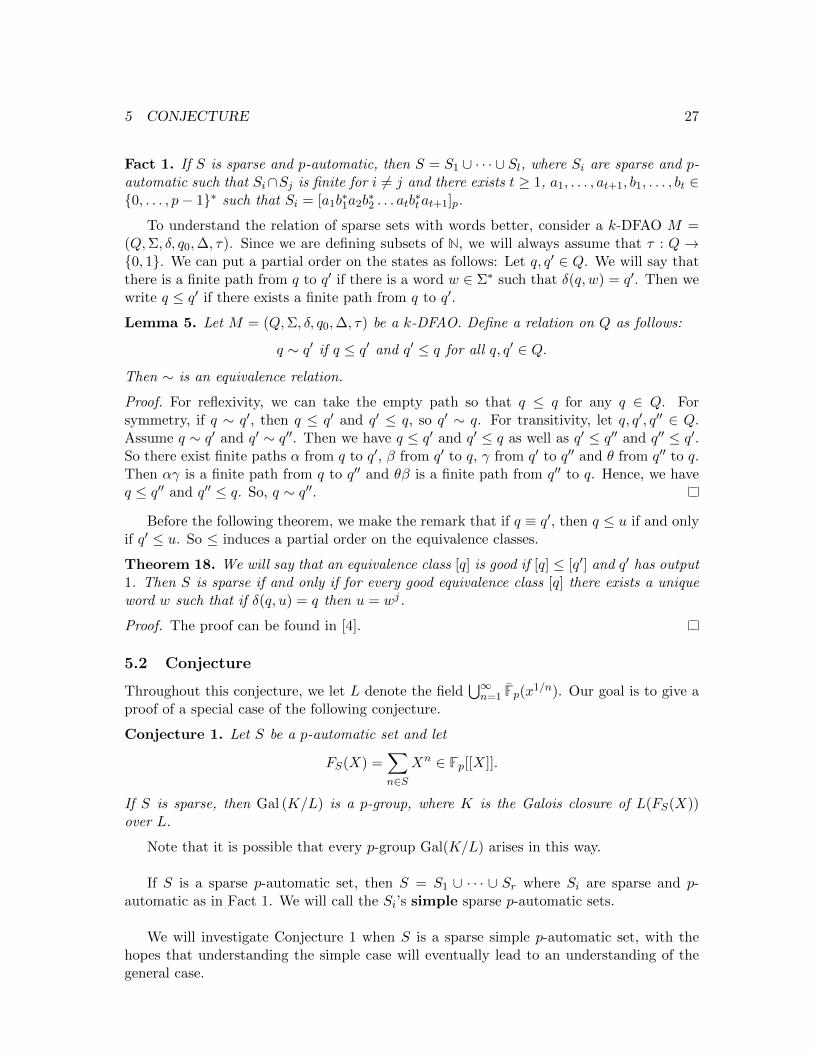
5 CONJECTURE 27
Fact 1. If S is sparse and p-automatic, then S = S1 ∪ · · · ∪ Sl, where Si are sparse and p-automatic such that Si∩Sj is finite for i 6= j and there exists t ≥ 1, a1, . . . , at+1, b1, . . . , bt ∈{0, . . . , p− 1}∗ such that Si = [a1b
∗1a2b
∗2 . . . atb
∗tat+1]p.
To understand the relation of sparse sets with words better, consider a k-DFAO M =(Q,Σ, δ, q0,∆, τ). Since we are defining subsets of N, we will always assume that τ : Q →{0, 1}. We can put a partial order on the states as follows: Let q, q′ ∈ Q. We will say thatthere is a finite path from q to q′ if there is a word w ∈ Σ∗ such that δ(q, w) = q′. Then wewrite q ≤ q′ if there exists a finite path from q to q′.
Lemma 5. Let M = (Q,Σ, δ, q0,∆, τ) be a k-DFAO. Define a relation on Q as follows:
q ∼ q′ if q ≤ q′ and q′ ≤ q for all q, q′ ∈ Q.
Then ∼ is an equivalence relation.
Proof. For reflexivity, we can take the empty path so that q ≤ q for any q ∈ Q. Forsymmetry, if q ∼ q′, then q ≤ q′ and q′ ≤ q, so q′ ∼ q. For transitivity, let q, q′, q′′ ∈ Q.Assume q ∼ q′ and q′ ∼ q′′. Then we have q ≤ q′ and q′ ≤ q as well as q′ ≤ q′′ and q′′ ≤ q′.So there exist finite paths α from q to q′, β from q′ to q, γ from q′ to q′′ and θ from q′′ to q.Then αγ is a finite path from q to q′′ and θβ is a finite path from q′′ to q. Hence, we haveq ≤ q′′ and q′′ ≤ q. So, q ∼ q′′.
Before the following theorem, we make the remark that if q ≡ q′, then q ≤ u if and onlyif q′ ≤ u. So ≤ induces a partial order on the equivalence classes.
Theorem 18. We will say that an equivalence class [q] is good if [q] ≤ [q′] and q′ has output1. Then S is sparse if and only if for every good equivalence class [q] there exists a uniqueword w such that if δ(q, u) = q then u = wj.
Proof. The proof can be found in [4].
5.2 Conjecture
Throughout this conjecture, we let L denote the field⋃∞n=1 Fp(x1/n). Our goal is to give a
proof of a special case of the following conjecture.
Conjecture 1. Let S be a p-automatic set and let
FS(X) =∑n∈S
Xn ∈ Fp[[X]].
If S is sparse, then Gal (K/L) is a p-group, where K is the Galois closure of L(FS(X))over L.
Note that it is possible that every p-group Gal(K/L) arises in this way.
If S is a sparse p-automatic set, then S = S1 ∪ · · · ∪ Sr where Si are sparse and p-automatic as in Fact 1. We will call the Si’s simple sparse p-automatic sets.
We will investigate Conjecture 1 when S is a sparse simple p-automatic set, with thehopes that understanding the simple case will eventually lead to an understanding of thegeneral case.
5 CONJECTURE 28
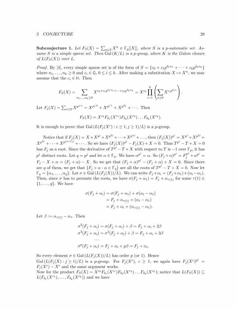
Subconjecture 1. Let FS(X) =∑
n∈S Xn ∈ Fp[[X]], where S is a p-automatic set. As-
sume S is a simple sparse set. Then Gal (K/L) is a p-group, where K is the Galois closureof L(FS(X)) over L.
Proof. By [4], every simple sparse set is of the form of S = {c0 + c1pδ1n1 + · · · + ckp
δknk}where n1, . . . , nk ≥ 0 and ci ∈ Q, 0 ≤ i ≤ k. After making a substitution X 7→ Xn, we mayassume that the ci ∈ N. Then
FS(X) =∑
n1,...,nk≥0Xc0+c1pδ1n1+···+ckpδknk = Xc0
k∏i=1
∑n≥0
Xcipδin
.
Let Fj(X) =∑
n≥0Xpj·n = Xpj·0 +Xpj·1 +Xp2j + · · · . Then
FS(X) = Xc0Fδ1(Xc1)Fδ2(Xc2) . . . Fδk(Xck).
It is enough to prove that Gal (L(Fj(Xc) : c ≥ 1, j ≥ 1)/L) is a p-group.
Notice that if Fj(X) = X+Xpj +Xp2j + · · ·+Xpnj + . . . , then (Fj(X))pj
= Xpj +Xp2j +
Xp3j + · · ·+Xp(n+1)j+ · · · . So we have (Fj(X))p
j −Fj(X) +X = 0. Thus T pj −T +X = 0
has Fj as a root. Since the derivative of T pj −T +X with respect to T is −1 over Fp, it has
pj distinct roots. Let q = pj and let α ∈ Fq. We have αpj
= α. So (Fj +α)pj
= F pj
j +αpj
=
Fj −X + α = (Fj + α) −X. So we get that (Fj + α)pj − (Fj + α) + X = 0. Since there
are q of them, we get that {Fj + α : α ∈ Fq} are all the roots of T pj − T +X = 0. Now let
Fq = {α1, . . . , αq}. Let σ ∈ Gal (L(Fj(X))/L). We can write Fj+αi = (Fj+α1)+(αi−α1).Then, since σ has to permute the roots, we have σ(Fj + α1) = Fj + ατ(1) for some τ(1) ∈{1, . . . , q}. We have
σ(Fj + αi) = σ(Fj + α1) + σ(αi − α1)
= Fj + ατ(1) + (αi − α1)
= Fj + αi + (ατ(1) − α1).
Let β := ατ(1) − α1. Then
σ2(Fj + αi) = σ(Fj + αi) + β = Fj + αi + 2β
σ3(Fj + αi) = σ2(Fj + αi) + β = Fj + αi + 3β
· · ·σp(Fj + αi) = Fj + αi + pβ = Fj + αi.
So every element σ ∈ Gal (L(Fj(X))/L) has order p (or 1). Hence
Gal (L(Fj(X) : j ≥ 1)/L) is a p-group. For Fj(Xc), c ≥ 1, we again have Fj(X
c)pj
=Fj(X
c)−Xc and the same argument works.Now for the product FS(X) = Xc0Fδ1(Xc1)Fδ2(Xc2) . . . Fδk(Xck); notice that L(FS(X)) ⊆L(Fδ1(Xc1), . . . , Fδk(Xck)) and we have
5 CONJECTURE 29
L,
K
F := L(Fδ1(Xc1), . . . , Fδk(Xck))
where K is the Galois closure of L(FS(X)) over L.In each Gal (L(Fδi(X
ci))/L) for 1 ≤ i ≤ k, every non-trivial element has order p. Henceevery element in Gal (L(Fδ1(Xc1), . . . , Fδk(Xck))/L) has order 1 or p. By the fundamentaltheorem of Galois theory, we have
Gal (F/L)/Gal (F/K) = Gal (K/L) .
We have just shown that Gal (F/L) is a p-group. A quotient of a p-group is also a p-groupand we are done.
Example 17. Let p = 2. Let S = {1, 2, 4, 8, 16, . . . } and F (X) =∑
n∈S Xn. Define
K := F2(X)(F (X)). We want to look at Gal(K/F2(X)
)= {σ : K → K : σ |F2(X)= id}.
Notice that F (X) is a root for the polynomial Y 2 − Y + X = 0 over F2(X). We look atF (X) + 1:
(F (X) + 1)2 − (F (X) + 1) +X = F (X)2 + 1− F (X)− 1 +X = F (X)2 − F (X) +X = 0.
So |Gal(K/F2(X)| = [K : F2(X)] = 2. Hence Gal(K/F2(X)
) ∼= Z/2Z. Hence the Galoisgroup is a 2-group.
Example 18. Let an =∑n
k=0 32k. So, we have a0 = 1, a1 = 1+32 = 10, a2 = 1+32+34 =91, . . . . Define S = {k ∈ N : k = an for some n}. Observe that S is sparse 3-automatic byFact 1. Then FS(X) = X + X10 + X91 + X820 · · · = X
(1 +X9 +X90 +X819 + · · ·
). Let
F (X) = 1 +X9 +X90 +X819 + · · · . Note that
(F (X))32
= X9 +X90 +X819 + · · ·= F (X)− 1.
So, F (X) is a root for the polynomial T 9 − T + 1. Let q = 32. Let α ∈ Fq. Then overF3(X),
(F (X) + α)32
− (F (X) + α) + 1 = (F (X))32
− F (X) + 1 + α− α = 0.
So, G := Gal(F3(X)(F (X))
/F3(X)
)is a p-group with |G| = 32. Denote E := F3(X)(F (X)),
K Galois closure of F3(X)(FS(X)) over F3(X) and F := F3(X). Then since we have
Gal(E/F )/Gal(E/K) = Gal(K/F ),
we get that Gal(K/
F3(X))
is a 3-group.
REFERENCES 30
References
[1] Boris Adamczewski, Jason P. Bell. Diagonalization and Rationalization of AlgebraicLaurent Series. Ann. Sci. Ec. Norm. Super. (4) 46, no. 6, 963–1004, 2013.
[2] Jean-Paul Allouche and Jeffrey Shallit. Automatic Sequences Theory, Applications, Gen-eralizations. Cambridge University Press, 2003.
[3] Jason P. Bell. A Gap Result for the Norms of Semigroups of Matrices. Linear Algebraand its Applications 402, 101–110, 2005.
[4] Jason P. Bell, Rahim Moosa. F -sets, Automaticity and Normality, in preparation.
[5] Gilles Christol. Ensembles presque periodiques k-reconnaissable. Theoret. Comput. Sci.9, no. 1, 141–145, 1979.
[6] Alan Cobham. Uniform Tag Sequences Math. Systems Theory 6, 164–192, 1972.
[7] Max Euwe. Mengentheoretische Betrachtungen uber das Schachspiel. Proc. Konin. Akad.Wetenschappen. 32 (5), Amsterdam., 633–642, 1929.
[8] Harry Furstenberg. Algebraic functions over finite fields. Journal of Algebra 7, 271–277,1967.
[9] Edouard Lucas. Theorie des Fonctions Numeriques Simplement Periodiques. AmericanJournal of Mathematics. 1 (2), 184–196,1878.
[10] Kurt Mahler. On the translation properties of a simple class of arithmetical functions.J. Math. and Physics 6, 158–163, 1927.
[11] Warren S. McCulloch, Walter H. Pitts. A logical calculus of the ideas immanent innervous activity. Bulletin of Mathematical Biophysics, Vol. 5, 115-133, 1943.
[12] George H. Mealy. A method for synthesizing sequential circuits. Bell System Tech. J.34, 1045–1079, 1955.
[13] Marston Morse. Recurrent geodesics on a surface of negative curvature. Transactionsof the American Mathematical Society , 22, 84–100, 1921.
[14] Olivier Salon. Suites automatiques a multi-indices et algebricite. C. R. Acad. Sci. ParisSr. I Math. 305, no. 12, 501–504, 1987.
[15] Richard P. Stanley. Enumerative Combinatorics 1. Cambridge Studies in AdvancedMathematics 49, 1997.
[16] Axel Thue. Uber die gegenseitige Lage gleicher Teile gewisser Zeichenreihen. SelectedMath. Papers of Axel Thue, Universiteitsforlaget, 67 pp, 1977.


![A Guide to Chess Endings [Max Euwe & David Hoper, 1959]](https://img.pdfslide.us/doc/110x75/55cf9919550346d0339b8b73/a-guide-to-chess-endings-max-euwe-david-hoper-1959.jpg)
![[M. M Botvinnik] Alekhine vs. Euwe Return Match 19(BookFi.org)](https://img.pdfslide.us/doc/110x75/577cd2de1a28ab9e78963257/m-m-botvinnik-alekhine-vs-euwe-return-match-19bookfiorg.jpg)