Embed Size (px)
DESCRIPTION
Fingleton Slides Peebles2009
Citation preview
7/21/2019 Fingleton Slides Peebles2009
http://slidepdf.com/reader/full/fingleton-slides-peebles2009 1/41
Spatial econometrics in about
40 minutesBernard Fingleton
University of Strathclyde

7/21/2019 Fingleton Slides Peebles2009
http://slidepdf.com/reader/full/fingleton-slides-peebles2009 2/41
Spatial econometrics in about 40minutes
• Why spatial econometrics?
• Spatial economics now widely recognised in theeconomics mainstream
• rugman!s "obel pri#e for wor$ on economic geography
• %mportance of networ$ economics &eg 'oyal (conomicSociety (aster )00* School + on ,-uctions and"etwor$s!.
• /S( (S' entre for Spatial (conomics
• %ncreasing policy relevance 1 World Ban$ &)002.+ WorldDevelopment Report 2009, World Ban$+ Washington3
• he standard time series econometric tools are notrelevant for spatial series
7/21/2019 Fingleton Slides Peebles2009
http://slidepdf.com/reader/full/fingleton-slides-peebles2009 3/41
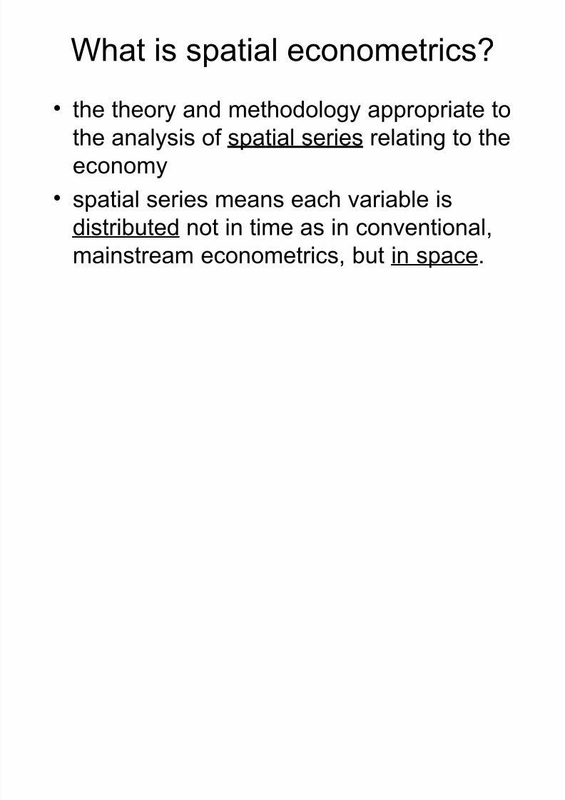
What is spatial econometrics?
• the theory and methodology appropriate tothe analysis of spatial series relating to theeconomy
• spatial series means each variable isdistributed not in time as in conventional+mainstream econometrics+ but in space3
7/21/2019 Fingleton Slides Peebles2009
http://slidepdf.com/reader/full/fingleton-slides-peebles2009 4/41
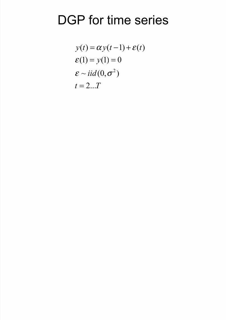
567 for time series
2
( ) ( 1) ( )
(1) (1) 0
~ (0, )2...
y t y t t
y
iid t T
α ε
ε
ε σ
= − +
= =
=
7/21/2019 Fingleton Slides Peebles2009
http://slidepdf.com/reader/full/fingleton-slides-peebles2009 5/41
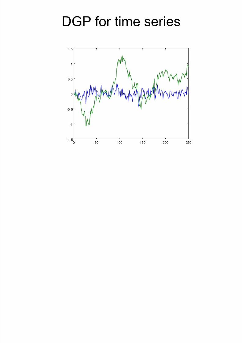
567 for time series
0 50 100 150 200 250-1.5
-1
-0.5
0
0.5
1
1.5
7/21/2019 Fingleton Slides Peebles2009
http://slidepdf.com/reader/full/fingleton-slides-peebles2009 6/41
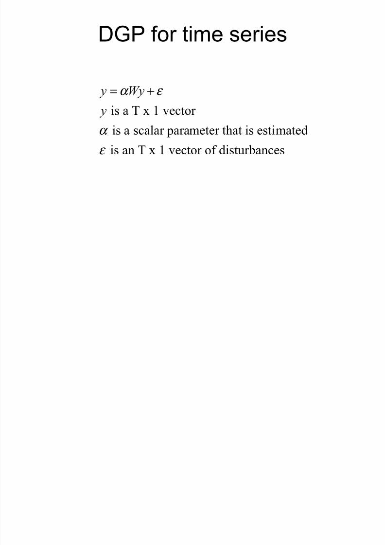
567 for time series
is a T x 1 vector
is a scalar parameter that is estimated
is an T x 1 vector of disturbances
y Wy
y
α ε
α
ε
= +
7/21/2019 Fingleton Slides Peebles2009
http://slidepdf.com/reader/full/fingleton-slides-peebles2009 7/41
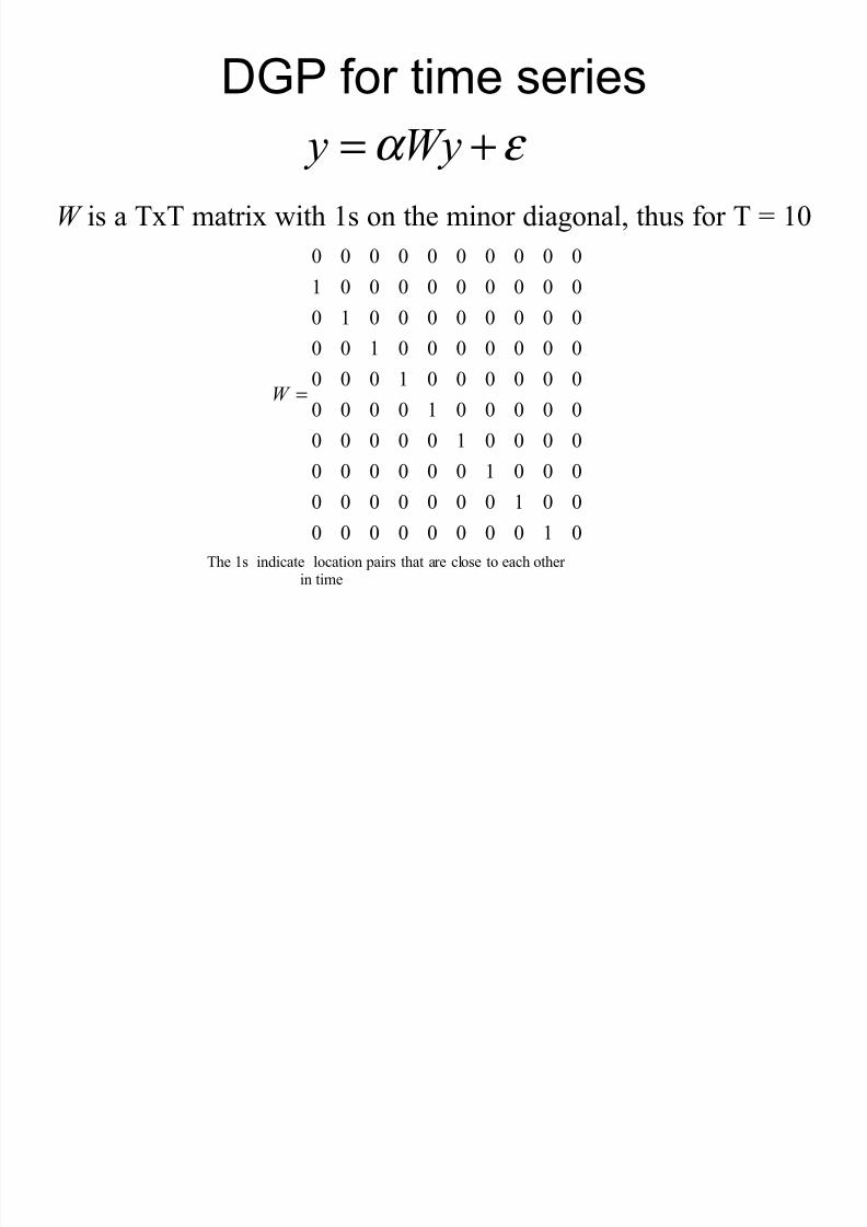
567 for time series
y Wyα ε = +
0 0 0 0 0 0 0 0 0 0
1 0 0 0 0 0 0 0 0 0
0 1 0 0 0 0 0 0 0 0
0 0 1 0 0 0 0 0 0 0
0 0 0 1 0 0 0 0 0 0
0 0 0 0 1 0 0 0 0 0
0 0 0 0 0 1 0 0 0 0
0 0 0 0 0 0 1 0 0 0
0 0 0 0 0 0 0 1 0 0
0 0 0 0 0 0 0 0 1 0
W =
W is a TxT matrix with 1s on the minor diagonal, thus for T 10
The 1s indicate location pairs that are close to each otherin time

7/21/2019 Fingleton Slides Peebles2009
http://slidepdf.com/reader/full/fingleton-slides-peebles2009 8/41
567 for time series
y Wyα ε = +
!rovided Wy and ε are contemporaneousl" independentwe can estimateα b" #$% and get consistent estimates,
although there is small sample bias.
7/21/2019 Fingleton Slides Peebles2009
http://slidepdf.com/reader/full/fingleton-slides-peebles2009 9/41
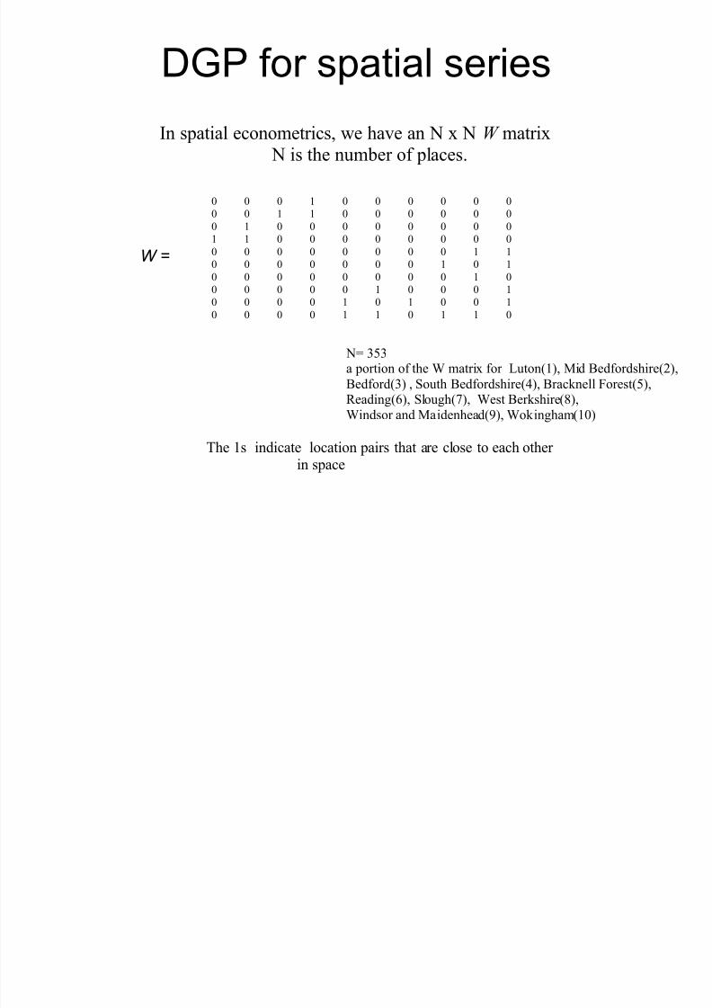
567 for spatial series
&n spatial econometrics, we have an ' x ' W matrix ' is the number of places.
The 1s indicate location pairs that are close to each other
in space
' a portion of the * matrix for $uton(1), +id edfordshire(2),
edford() , %outh edfordshire(-), racnell /orest(),eading(), %lough(), *est ershire(3),*indsor and +aidenhead(4), *oingham(10)
0 0 0 1 0 0 0 0 0 00 0 1 1 0 0 0 0 0 0
0 1 0 0 0 0 0 0 0 01 1 0 0 0 0 0 0 0 0
0 0 0 0 0 0 0 0 1 10 0 0 0 0 0 0 1 0 1
0 0 0 0 0 0 0 0 1 00 0 0 0 0 1 0 0 0 10 0 0 0 1 0 1 0 0 1
0 0 0 0 1 1 0 1 1 0
W 8
7/21/2019 Fingleton Slides Peebles2009
http://slidepdf.com/reader/full/fingleton-slides-peebles2009 10/41
567 for spatial series5istrict3shp
4090: ; 2*0<:
2*0<: ; <)**==
<)**== ; <9=:4*
<9=:4* ; )94:*>
)94:*> ; =:*04*
'esidential property prices in (ngland+ )00<
'

7/21/2019 Fingleton Slides Peebles2009
http://slidepdf.com/reader/full/fingleton-slides-peebles2009 11/41
567 for spatial series
is an ' x 1 vector
is a scalar parameter that is estimated
is an ' x 1 vector of disturbances
y Wy
y
ρ ε
ρ
ε
= +

7/21/2019 Fingleton Slides Peebles2009
http://slidepdf.com/reader/full/fingleton-slides-peebles2009 12/41
567 for spatial series
y Wy ρ ε = +
• This is an almost identical set5up to the time series case6nd one might thin that it can also be consistentl" estimated b" #$%
• ut now there is one big difference
• we cannot estimate the spatial autoregression b" #$%
and obtain consistent estimates of ρ .
• eason 5 Wy and ε are not independent.
• Wy determines y but is also determined b" y.
7/21/2019 Fingleton Slides Peebles2009
http://slidepdf.com/reader/full/fingleton-slides-peebles2009 13/41
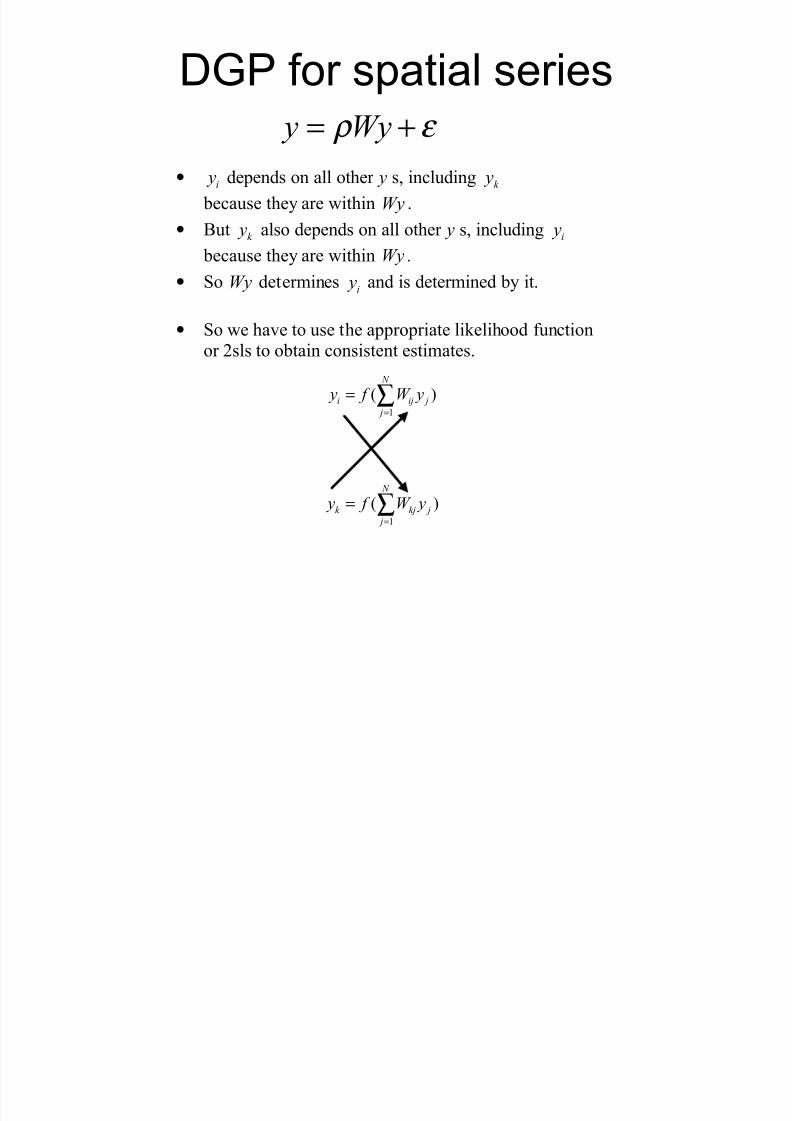
567 for spatial series
• i y depends on all other y s, including k y
because the" are within Wy .
• ut k y also depends on all other y s, including i y
because the" are within Wy .• %o Wy determines
i y and is determined b" it.
• %o we have to use the appropriate lielihood functionor 2sls to obtain consistent estimates.
y Wy ρ ε = +
1
( ) N
i ij j
j
y f W y=
= ∑
1
( ) N
k kj j
j
y f W y=
= ∑
7/21/2019 Fingleton Slides Peebles2009
http://slidepdf.com/reader/full/fingleton-slides-peebles2009 14/41
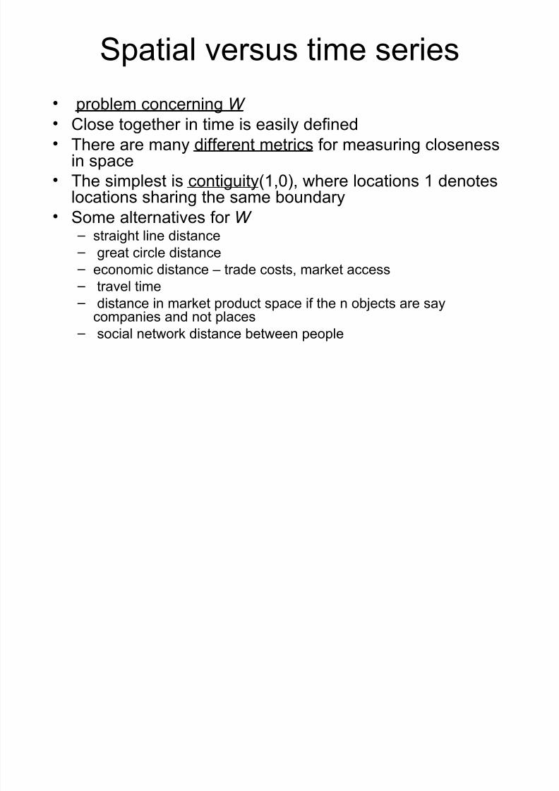
Spatial versus time series
• problem concerning W • lose together in time is easily defined• here are many different metrics for measuring closeness
in space
• he simplest is contiguity&<+0.+ where locations < denoteslocations sharing the same boundary• Some alternatives for W
straight line distance great circle distance
economic distance trade costs+ mar$et access travel time distance in mar$et product space if the n ob@ects are say
companies and not places social networ$ distance between people

7/21/2019 Fingleton Slides Peebles2009
http://slidepdf.com/reader/full/fingleton-slides-peebles2009 15/41
Some typical models
7/21/2019 Fingleton Slides Peebles2009
http://slidepdf.com/reader/full/fingleton-slides-peebles2009 16/41
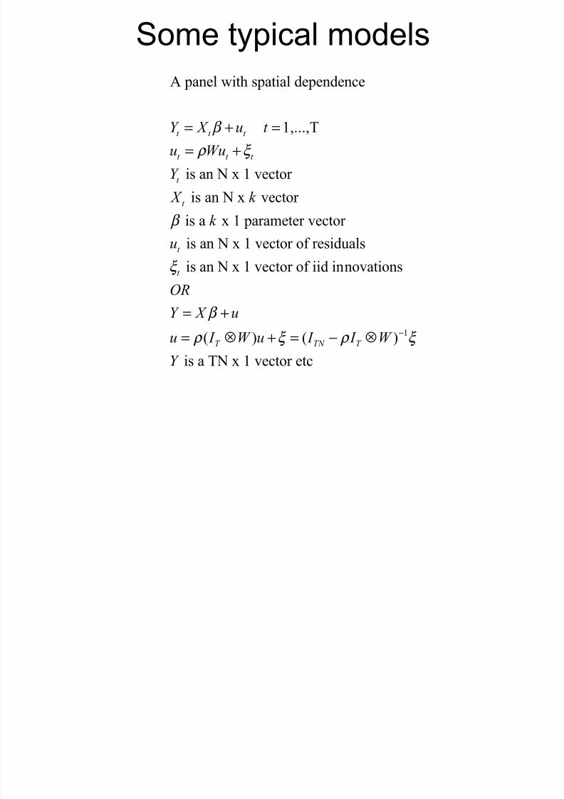
Some typical models
6 panel with spatial dependence
1,...,T
is an ' x 1 vector
is an ' x vector
is a x 1 parameter vector
is an ' x 1 vector of residuals
is an ' x 1 vector of iid in
t t t
t t t
t
t
t
t
Y X u t
u Wu
Y
X k
k
u
β
ρ ξ
β
ξ
= + =
= +
1
novations
( ) ( )
is a T' x 1 vector etc
T TN T
OR
Y X u
u I W u I I W
Y
β
ρ ξ ρ ξ −
= +
= ⊗ + = − ⊗

7/21/2019 Fingleton Slides Peebles2009
http://slidepdf.com/reader/full/fingleton-slides-peebles2009 17/41
(stimation
• A/ typically used but problems33
"o large sample theory
Fails to handle other endogenous variableson rhs+ i3e3 eCcluding spatial lag &Wy .
-ssumes normality+ or some other specificdistribution+ )S/SD6A robust
A/ reEuires eigenvalues of W matriC+ if "large this may be problematic

7/21/2019 Fingleton Slides Peebles2009
http://slidepdf.com/reader/full/fingleton-slides-peebles2009 18/41
Some typical models

7/21/2019 Fingleton Slides Peebles2009
http://slidepdf.com/reader/full/fingleton-slides-peebles2009 19/41
(stimationT"picall" these models are estimated b" +$.
7owever another ver" useful method to estimate these models is /8%2%$%
or feasible generalised spatial 2 stage least s9uares.
The method involves stages.
• %tage 1 the model is estimated b" 2%$% to obtain :β .• %tage 2 the resulting 2%$% residuals give :λ and 2:σ using a 8+ procedure.
• %tage :λ is used to perform a ;ochrane5#rcutt5t"pe transformation
to account for the spatial dependence in the residuals,
to obtain
::β .
This is the most sensible single e9uation estimation method with
endogenous right hand side regressors (in addition to WY ) included within X .

7/21/2019 Fingleton Slides Peebles2009
http://slidepdf.com/reader/full/fingleton-slides-peebles2009 20/41
Some applications
/ingleton (200b) <The new economic geograph" versus urban economics = anevaluation using local wage rates in 8reat ritain>, Oxford Economic Papers 3 015
0

7/21/2019 Fingleton Slides Peebles2009
http://slidepdf.com/reader/full/fingleton-slides-peebles2009 21/41
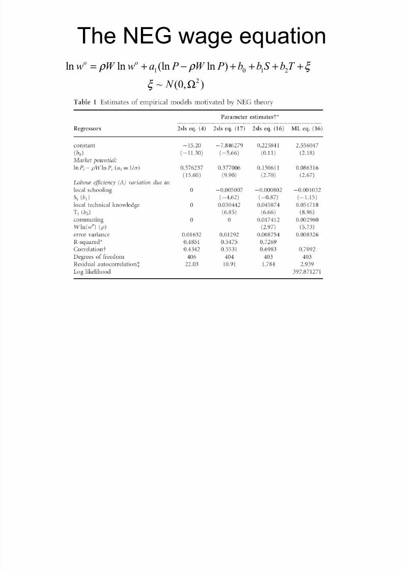
he "(6 wage eEuation
5istrict3shp
03=4> ; 032=>
032=> ; 03**)
03**) ; <3<2)
<3<2) ; <3>0=
<3>0= ; )349<
'elative wage rates5istrict3shp
034<= ; 0392)
0392) ; 03*=
03*= ; <3<:>
<3<:> ; <3:9:
<3:9: ; <322:
'elative mar$et potential

7/21/2019 Fingleton Slides Peebles2009
http://slidepdf.com/reader/full/fingleton-slides-peebles2009 22/41
he "(6 wage eEuation
1 0 1 2
2
ln ln (ln ln )
~ (0, )
o ow W w a P W P ! T
N
ρ ρ ξ
ξ
= + − + + + +
Ω
7/21/2019 Fingleton Slides Peebles2009
http://slidepdf.com/reader/full/fingleton-slides-peebles2009 23/41
he "(6 wage eEuation
1 0 1 2
2
ln ln (ln ln )
~ (0, )
o o
w W w a P W P ! T
N ρ ρ ξ
ξ = + − + + + +
Ω
7/21/2019 Fingleton Slides Peebles2009
http://slidepdf.com/reader/full/fingleton-slides-peebles2009 24/41
Some applications
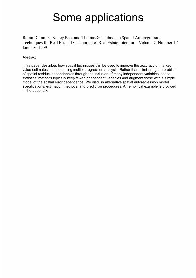
obin ?ubin, . @elle" !ace and Thomas 8. Thibodeau %patial 6utoregressionTechni9ues for eal Astate ?ata Bournal of eal Astate $iterature Colume , 'umber 1 D
Banuar", 1444
-bstract
his paper describes how spatial techniEues can be used to improve the accuracy of mar$etvalue estimates obtained using multiple regression analysis3 'ather than eliminating the problemof spatial residual dependencies through the inclusion of many independent variables+ spatialstatistical methods typically $eep fewer independent variables and augment these with a simplemodel of the spatial error dependence3 We discuss alternative spatial autoregression modelspecifications+ estimation methods+ and prediction procedures3 -n empirical eCample is providedin the appendiC3

7/21/2019 Fingleton Slides Peebles2009
http://slidepdf.com/reader/full/fingleton-slides-peebles2009 25/41
Some applications
eron @ et al (200-) 7edonic price functions and spatial dependence = implications forthe demand for urban air 9ualit", ;hapter 12 in 6dvances in %patial Aconometrics (Ads
6nslin, $ /lorax and e" %) %pringer.
in <*=9 'onald 'id$er and ohn Genning conducted the first study that lin$ed air pollution to
property prices3 33there seems to be a preponderance of evidence that air pollution is negativelyrelated to house prices3 his is important because it reveals information about the willingness topay for air Euality a non;mar$et commodity3 much of the analysis focuses on the hedonicregressions+ wherein some measure of house price is the dependent variable and measures ofthe characteristics of housing H eg living area+ eCistence of a pool+ neighbourhood Euality+ schooldistrict as well as measures of pollution are the independent variables33we are worried that thepotential for misspecifying the role of neighbourhood Euality as a determinant of house prices ishigh3 For us this is relevant to the eCtent that it may significantly alter the estimate of the airpollution effect33to analyse these issues we use the tools of spatial econometrics3

7/21/2019 Fingleton Slides Peebles2009
http://slidepdf.com/reader/full/fingleton-slides-peebles2009 26/41
Some applications
@im ; *, !hipps, T, 6nselin, $ (200) +easuring the benefits of air 9ualit"improvement= a spatial hedonic approach, "ourna# of En$ironmenta# Economics and
%ana&ement , - 2-54
Abstract: he primary ob@ective of this paper is to improve the methodology for estimating hedonic price
functions when the data are inherently spatial3 - spatial;econometric hedonic housing pricemodel is developed and estimated for the Seoul metropolitan area to measure the marginal valueof improvements in SI) and "IJ concentrations3 5iagnostic testing favored the spatial lagmodel over the spatial error model3 'esults showed that SI) pollution levels had a significantimpact on housing prices while "IJ pollution did not3 he authors attribute this differential impactto the relatively higher levels of SI) pollution when compared with pollution standards and therelative recency of "IJ pollution3 Aarginal W7 for a 4K improvement in mean SI)concentrations is about L)+::: or <34K of mean housing price3

7/21/2019 Fingleton Slides Peebles2009
http://slidepdf.com/reader/full/fingleton-slides-peebles2009 27/41
Some applications
Bernard Fingleton and Julie Le Gallo
"Estimating spatial models with endogenous variables, a spatial
lag and spatially dependent disturbances: Finite sampleproperties“
apers in !egional cience, #olume $%, &umber ', (ugust )**$+
!esults can be replicated in tata

7/21/2019 Fingleton Slides Peebles2009
http://slidepdf.com/reader/full/fingleton-slides-peebles2009 28/41
Some applications
http:www+sml+hw+ac+u-ecomespeebles
.ontains tata data /ile
tata do /ile
tata log /ile

7/21/2019 Fingleton Slides Peebles2009
http://slidepdf.com/reader/full/fingleton-slides-peebles2009 29/41
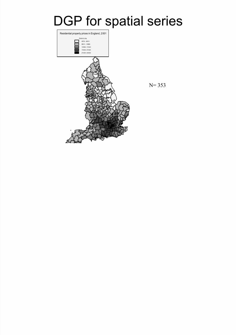
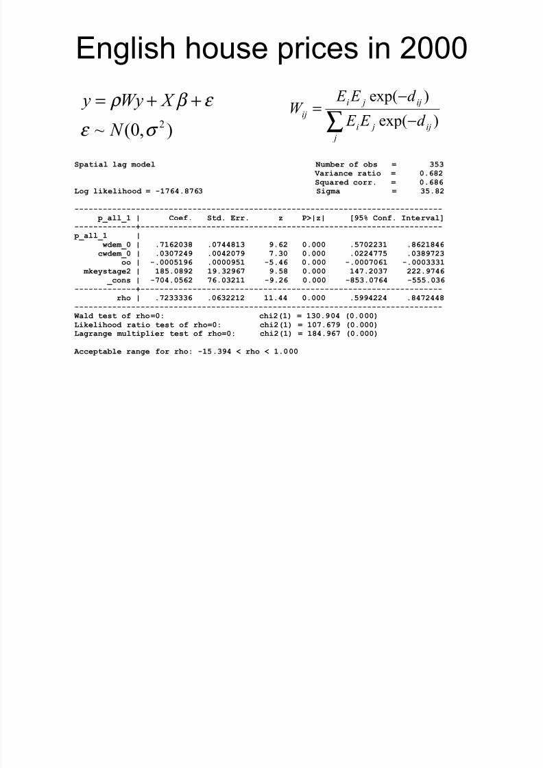
(nglish house prices in )0005istrict3shp
4090: ; 2*0<:
2*0<: ; <)**==
<)**== ; <9=:4*
<9=:4* ; )94:*>
)94:*> ; =:*04*
'esidential property prices in (ngland+ )00<
'
7/21/2019 Fingleton Slides Peebles2009
http://slidepdf.com/reader/full/fingleton-slides-peebles2009 30/41
(nglish house prices in )000
2~ (0, )
y Wy X
N
ρ β ε
ε σ
= + +
Spatial lag model Number of obs = 353 Variance ratio = 0.682Squared corr. = 0.686
Log lieli!ood = "#$6%.8$63 Sigma = 35.82
"""""""""""""""""""""""""""""""""""""""""""""""""""""""""""""""""""""""""""""" p&all&# ' (oef. Std. )rr. * +,'*' -5/ (onf. nter1al
""""""""""""""""""""""""""""""""""""""""""""""""""""""""""""""""""""""""""""" p&all&# '
4dem&0 ' .$#62038 .0$%%8#3 .62 0.000 .5$0223# .862#8%6c4dem&0 ' .030$2% .00%20$ $.30 0.000 .022%$$5 .038$23
oo ' ".0005#6 .00005# "5.%6 0.000 ".000$06# ".000333# mestage2 ' #85.082 #.326$ .58 0.000 #%$.203$ 222.$%6
&cons ' "$0%.0562 $6.032## ".26 0.000 "853.0$6% "555.036"""""""""""""""""""""""""""""""""""""""""""""""""""""""""""""""""""""""""""""
r!o ' .$233336 .06322#2 ##.%% 0.000 .5%22% .8%$2%%8"""""""""""""""""""""""""""""""""""""""""""""""""""""""""""""""""""""""""""""" ald test of r!o=07 c!i2#9 = #30.0% 0.0009Lieli!ood ratio test of r!o=07 c!i2#9 = #0$.6$ 0.0009Lagrange multiplier test of r!o=07 c!i2#9 = #8%.6$ 0.0009
:cceptable range for r!o7 "#5.3% ; r!o ; #.000
exp( )
exp( )
i j ij
ij
i j ij
j
E E d W
E E d
−=
−∑
7/21/2019 Fingleton Slides Peebles2009
http://slidepdf.com/reader/full/fingleton-slides-peebles2009 31/41
567 for spatial series
The 1s indicate location pairs that are close to each other
in space
' a portion of the * matrix for $uton(1), +id edfordshire(2),
edford() , %outh edfordshire(-), racnell /orest(),eading(), %lough(), *est ershire(3),*indsor and +aidenhead(4), *oingham(10)
0 0 0 1 0 0 0 0 0 00 0 1 1 0 0 0 0 0 0
0 1 0 0 0 0 0 0 0 0
1 1 0 0 0 0 0 0 0 00 0 0 0 0 0 0 0 1 10 0 0 0 0 0 0 1 0 1
0 0 0 0 0 0 0 0 1 00 0 0 0 0 1 0 0 0 10 0 0 0 1 0 1 0 0 1
0 0 0 0 1 1 0 1 1 0
W* 8
7/21/2019 Fingleton Slides Peebles2009
http://slidepdf.com/reader/full/fingleton-slides-peebles2009 32/41
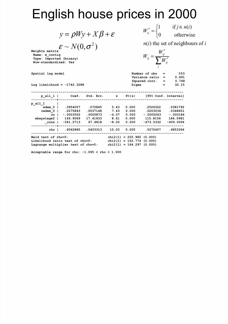
(nglish house prices in )000
2~ (0, )
y Wy X
N
ρ β ε
ε σ
= + +
eig!ts matri< Name7 4&contigpe7 mported binar9>o4"standardi*ed7 ?es
Spatial lag model Number of obs = 353 Variance ratio = 0.6#Squared corr. = 0.$%8
Log lieli!ood = "#$%2.3288 Sigma = 32.#5
"""""""""""""""""""""""""""""""""""""""""""""""""""""""""""""""""""""""""""""" p&all&# ' (oef. Std. )rr. * +,'*' -5/ (onf. nter1al
""""""""""""""""""""""""""""""""""""""""""""""""""""""""""""""""""""""""""""" p&all&# '
4dem&0 ' .35%05$ .0$28%5 5.%3 0.000 .2526322 .538#$2c4dem&0 ' .02$58%3 .003$#%8 $.%3 0.000 .020303% .03%865#
oo ' ".0003552 .00008$3 "%.0$ 0.000 ".0005263 ".000#8% mestage2 ' #%.56 #$.%#33 8.6# 0.000 ##5.8#56 #8%.08#
&cons ' "5%#.2$#3 6$.%8#8 "8.02 0.000 "6$3.5332 "%0.00%"""""""""""""""""""""""""""""""""""""""""""""""""""""""""""""""""""""""""""""
r!o ' .6062885 .0%033#3 #5.03 0.000 .52$2%0$ .685336%""""""""""""""""""""""""""""""""""""""""""""""""""""""""""""""""""""""""""""""
ald test of r!o=07 c!i2#9 = 225.82 0.0009Lieli!ood ratio test of r!o=07 c!i2#9 = #52.$$% 0.0009Lagrange multiplier test of r!o=07 c!i2#9 = #6%.2$ 0.0009
:cceptable range for r!o7 "#.05 ; r!o ; #.000
E
E
E
1 if ( )
0 otherwise
( ) the set of neighbours of
ij
ij
ij
ij
j
j n iW
n i i
W W
W
∈=
=∑

7/21/2019 Fingleton Slides Peebles2009
http://slidepdf.com/reader/full/fingleton-slides-peebles2009 33/41
(nglish house prices in )000
. @@@@@@@@@@@@@@@@@@@@@@@@@@@@@ >)A)>)N()7 BLS @@@@@@@@@@@@@@@@@@@@@@@@@@@@@@@.. @ :s abo1eC but estimating using BLS... regress p&all&# 4dem&0 c4dem&0 oo mestage2
Source ' SS df DS Number of obs = 353""""""""""""""""""""""""""""""""""""""""""" A %C 3%89 = ##6.2$
Dodel ' 82%8#2.#68 % 206203.0%2 +rob , A = 0.0000>esidual ' 6#$#88.856 3%8 #$$3.53## >"squared = 0.5$20
""""""""""""""""""""""""""""""""""""""""""" :dE >"squared = 0.56$#otal ' #%%200#.02 352 %06.5382 >oot DS) = %2.##3
"""""""""""""""""""""""""""""""""""""""""""""""""""""""""""""""""""""""""""""" p&all&# ' (oef. Std. )rr. t +,'t' -5/ (onf. nter1al
""""""""""""""""""""""""""""""""""""""""""""""""""""""""""""""""""""""""""""" 4dem&0 ' .86%005 .0862%6$ #0.02 0.000 .6%3$55 #.033636c4dem&0 ' .05$$055 .00%0$$ #%.08 0.000 .0%6%6# .065$6%
oo ' ".000$##2 .000##0# "6.%6 0.000 ".0002$8 ".000%%$ mestage2 ' #$5.802 22.$0$% $.$% 0.000 #3#.#%#$ 220.%6%#
&cons ' "5$#.8$%5 88.353% "6.%$ 0.000 "$%5.660# "38.08""""""""""""""""""""""""""""""""""""""""""""""""""""""""""""""""""""""""""""""
Y X β ε = +
7/21/2019 Fingleton Slides Peebles2009
http://slidepdf.com/reader/full/fingleton-slides-peebles2009 34/41
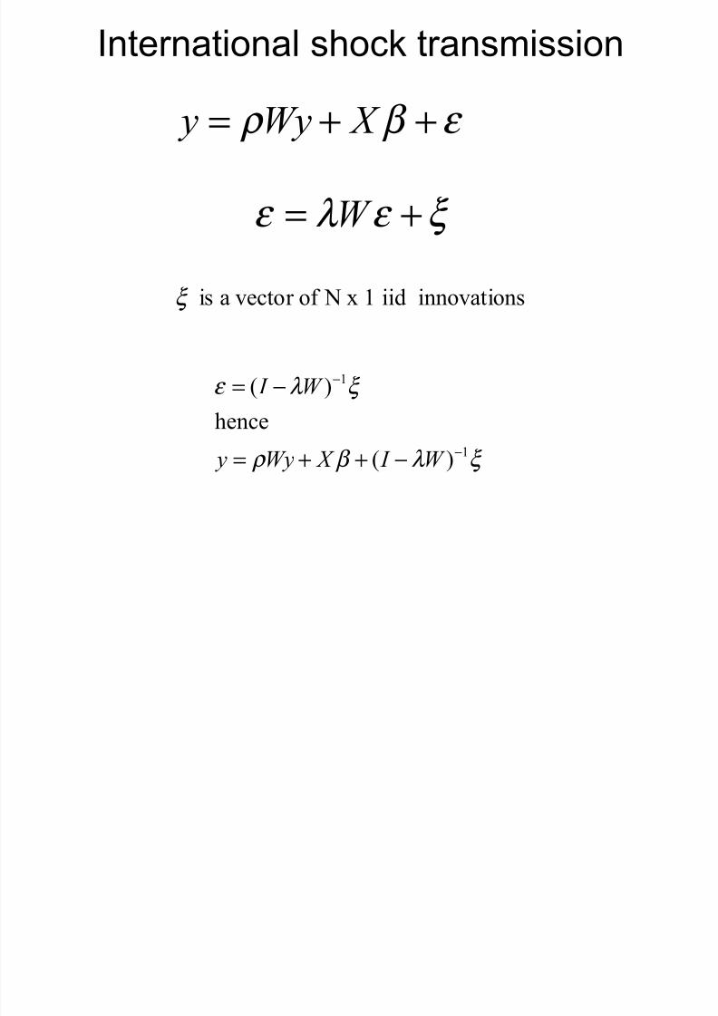
%nternational shoc$ transmission
ξ is a vector of ' x 1 iid innovations
1
1
( )
hence
( )
I W
y Wy X I W
ε λ ξ
ρ β λ ξ
−
−
= −
= + + −
y Wy X ρ β ε = + +
W ε λ ε ξ = +

7/21/2019 Fingleton Slides Peebles2009
http://slidepdf.com/reader/full/fingleton-slides-peebles2009 35/41
%nternational shoc$ transmission
ξ is a vector of ' x 1 iid innovations
1
1
( )
hence
( )
I W
y Wy X I W
ε λ ξ
ρ β λ ξ
−
−
= −
= + + −
6nd for λ F1
1 2 2
0
( ) ( ) ...i i
i
I W W W W W λ ξ λ ξ ξ λ ξ λ ξ λ ξ ∞
−
=
− = = + + + +∑
0W I = , 2W is the matrix product of W and W , and W i is the matrix product of W i51 and W .
*hich means a shoc at G goes to all other locations.

7/21/2019 Fingleton Slides Peebles2009
http://slidepdf.com/reader/full/fingleton-slides-peebles2009 36/41
%nternational shoc$ transmission6lternativel", we might invoe a moving average error process
( ) I W ε λ ξ = −
+6 errors impl" shocs that are onl" transmitted locall". This difference is highlighted b" this diagram
%hoc effects with 6 errors %hoc effects with +6 errors
7/21/2019 Fingleton Slides Peebles2009
http://slidepdf.com/reader/full/fingleton-slides-peebles2009 37/41
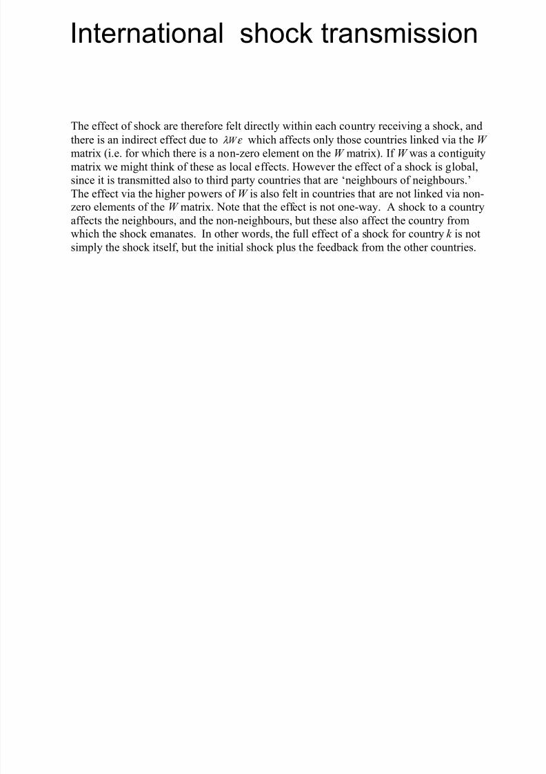
%nternational shoc$ transmission
The effect of shoc are therefore felt directl" within each countr" receiving a shoc, and
there is an indirect effect due to W λ ε which affects onl" those countries lined via the W
matrix (i.e. for which there is a non5Hero element on the W matrix). &f W was a contiguit"
matrix we might thin of these as local effects. 7owever the effect of a shoc is global,
since it is transmitted also to third part" countries that are <neighbours of neighbours.>The effect via the higher powers of W is also felt in countries that are not lined via non5Hero elements of the W matrix. 'ote that the effect is not one5wa". 6 shoc to a countr"
affects the neighbours, and the non5neighbours, but these also affect the countr" fromwhich the shoc emanates. &n other words, the full effect of a shoc for countr" k is not
simpl" the shoc itself, but the initial shoc plus the feedbac from the other countries.
7/21/2019 Fingleton Slides Peebles2009
http://slidepdf.com/reader/full/fingleton-slides-peebles2009 38/41
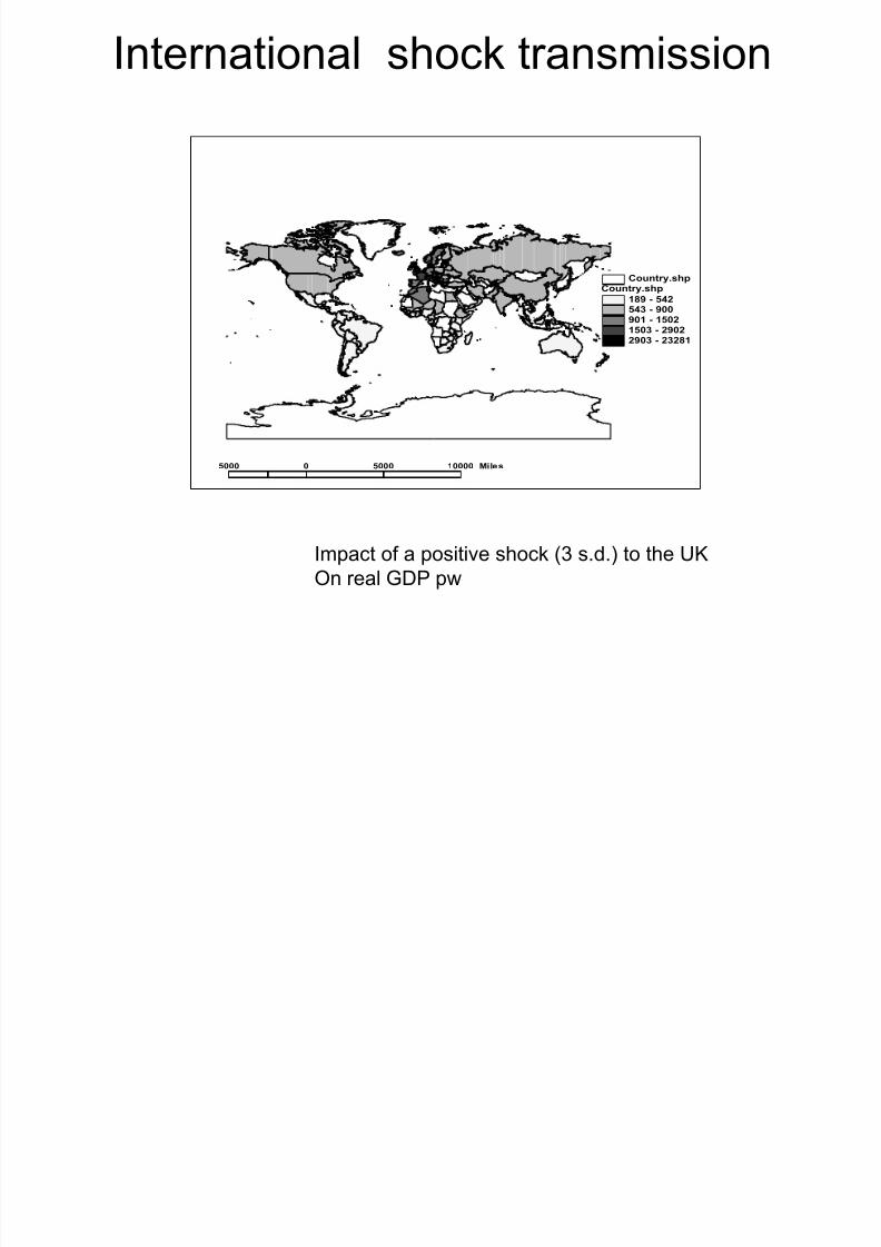
%nternational shoc$ transmission
%mpact of a positive shoc$ &: s3d3. to the U
In real 657 pw
.ountry+shp0$1 2 34)34' 2 1**1*0 2 03*)03*' 2 )1*))1*' 2 )')$0
.ountry+shp
3*** * 3*** 0**** 5iles
7/21/2019 Fingleton Slides Peebles2009
http://slidepdf.com/reader/full/fingleton-slides-peebles2009 39/41
spatial econometrics software
• A-/-B Aany routines available on ames /eSage!s
webpages
-dvanced spatial econometrics using A-/-B+available from
• http1DDwww3spatial;econometrics3comD
• Stata
Some routines forthcoming and available 5avid 5ru$$erMs pac$age3 When available+ hepac$age is described here1http1DDrepec3orgDsnasug02Ddru$$erNspatial3pdf 3

7/21/2019 Fingleton Slides Peebles2009
http://slidepdf.com/reader/full/fingleton-slides-peebles2009 40/41
ourse
• Second OSpatial (conometrics -dvanced %nstituteOthat will be held again in 'ome in -my;une )00*3he deadline for applications is the end of anuary3
-ll the details may be found at the website
Www3Spatialeconometricsadvancedinstitute3org

7/21/2019 Fingleton Slides Peebles2009
http://slidepdf.com/reader/full/fingleton-slides-peebles2009 41/41
boo$s
• -nselin / &<*22. Spatial Econometrics: Methodsand Models3 5ordrecht 1 luwer3
• -nselin / &)00<. Spatial (conometrics+ in B3 Baltagi&ed. A ompanion to !heoretical Econometrics+Blac$well1 ICford+ :<0;::0
• -nselin / &)00=. MSpatial econometricsM in Aillsand 7atterson &eds. "al#rave $andboo% o&Econometrics : vol ' Econometric theory 7algrave1Aacmillan )00= *0<;*=*

![Cytotechnology Volume 12 issue 1-3 1993 [doi 10.1007%2Fbf00744674] Susan McDonnell; Barbara Fingleton -- Role of matrix metalloproteinases in invasion, and metastasis- biology, diagnosis](https://img.pdfslide.us/doc/110x75/577cc1851a28aba711933fb9/cytotechnology-volume-12-issue-1-3-1993-doi-1010072fbf00744674-susan-mcdonnell.jpg)