Embed Size (px)
Citation preview

Introduction & motivation Results Math meets computers meet... Conclusion
Finding the optimal strategy in a tally gameCODY2010, November 2010
Neil Dobbs, Tomasz Nowicki, Maxim Sviridenko, GrzegorzSwirszcz
IBM – Watson Research Center
November 2010

Introduction & motivation Results Math meets computers meet... Conclusion
Tally Game
• ?• ‘a cruel, yet funny game played by employees in smaller
stores. to play, simply count the number of ugly, weird orgross people who come into the store with tally marks onreceipt paper. accompany your mark by quickly shouting"tally" or saying it loud enough to let your fellowworker-bees know an awful being had just graced yourestablishment with it’s yucky presence. the employee withthe most tally’sat the end of the day is the winner. and should be rewarded.’http://www.urbandictionary.com/define.php?term=tally20game
• ‘The score, or the stick with notches in it to keep a track ofthe score or count.’ Merriam Webster
• Gra w Karbowego Tomasz Nowicki

Introduction & motivation Results Math meets computers meet... Conclusion
Generalized Tally Game
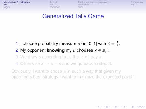
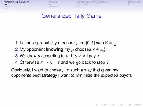
1 I choose probability measure µ on [0,1] with E = 12 .
2 My opponent knowing my µ chooses x ∈ R+0 .
3 We draw s according to µ. If s ≥ x I pay x .4 Otherwise x → x − s and we go back to step 3.
Obviously, I want to chose µ in such a way that given myopponents best strategy I want to minimize the expected payoff.
Introduction & motivation Results Math meets computers meet... Conclusion
Generalized Tally Game
1 I choose probability measure µ on [0,1] with E = 12 .
2 My opponent knowing my µ chooses x ∈ R+0 .
3 We draw s according to µ. If s ≥ x I pay x .4 Otherwise x → x − s and we go back to step 3.
Obviously, I want to chose µ in such a way that given myopponents best strategy I want to minimize the expected payoff.

Introduction & motivation Results Math meets computers meet... Conclusion
Joint Replenishment Problem with Time WindowsThis is one of the fundamental problems in Inventory andSupply Chain Management.• We are given a warehouse and the set of retailers{1, . . . ,n}.
• We are given the discrete time horizon {1, . . . ,T}.• We are given a set of demands D consisting of triples
(i , r , t) for retailer of type i that arrives at time t and mustbe satisfied by an order placed in the time interval [r , t ].
• To satisfy arbitrary many demands in some time period τ aretailer i places an order at warehouse at time τ and incursthe retailer ordering cost Ki , at the same time thewarehouse places an order and incurs the warehouseordering cost of K0. The goal is define the set set ofwarehouse and retailer orders to satisfy all the demand.

Introduction & motivation Results Math meets computers meet... Conclusion
IP Formulation & LP Relaxation•
minT∑τ=1
K0xτ0 +n∑
i=1
T∑τ=1
Kixτ i , (1.1)
t∑τ=r
xτ i ≥ 1, ∀(i , r , t) ∈ D, (1.2)
xτ i ≤ xτ0 ∀i , τ, (1.3)xτ0, xτ i ∈ {0,1}, ∀τ, i . (1.4)
• We relax the integrality condition (1.4) with the conditionxτ0, xτ i ∈ [0,1] for all τ, i and solve the resulting linearprogramming relaxation using any efficient algorithm(interior points, ellipsoid method). Let x∗ be an optimalsolution for the linear relaxation.

Introduction & motivation Results Math meets computers meet... Conclusion
Rounding Algorithm
Consider the following rounding algorithm that finds an integralsolution for our optimization problem:
1. Define intervals It = (∑t−1
τ=1 x∗τ0,∑t
τ=1 x∗τ0] for time t andintervals Iti = (
∑t−1τ=1 x∗τ i ,
∑tτ=1 x∗τ i ] for time t and retailer i .
2. Consecutively draw random variable di from the randomdistribution f (x). Define D0 = 0 and Di = Di−1 + di .
3. Let Λ be the set of times t such that there is an index i suchthat Di ∈ It . Open warehouse orders at all times from Λ.
4. For each retailer independently apply the followingprocess. Initialize y = 0. Open retailer i order at the latesttime t ′′ from Λ such that t ′′ ≤ t ′ where y + 1 ∈ It ′i . Sety =
∑tτ=1 x∗τ i and repeat the process until
y + 1 >∑T
τ=1 x∗τ i .

Introduction & motivation Results Math meets computers meet... Conclusion
Sketch of the Analysis
It is not hard to show that this algorithm finds a feasiblesolution. The expected cost of this solution is upper bounded by
W1
1− ρ(f )+
W2
α
where W1 =∑n
i=1∑T
τ=1 Kix∗τ i and W2 =∑T
τ=1 K0x∗τ i , i.e.W1 + W2 is the optimal cost of linear programming relaxation.

Introduction & motivation Results Math meets computers meet... Conclusion
Generalized Tally Game - revisited
1 I choose probability measure µ on [0,1] with E = 12 .
2 My opponent knowing my µ chooses x ∈ R+0 .
3 We draw s according to µ. If s ≥ x I pay x .4 Otherwise x → x − s and we go back to step 3.
Obviously, I want to chose µ in such a way that given myopponents best strategy I want to minimize the expected payoff.
Introduction & motivation Results Math meets computers meet... Conclusion
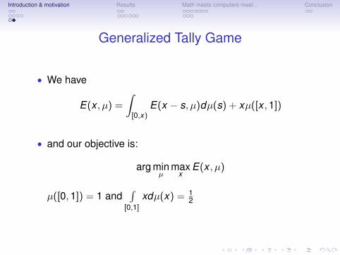
Generalized Tally Game
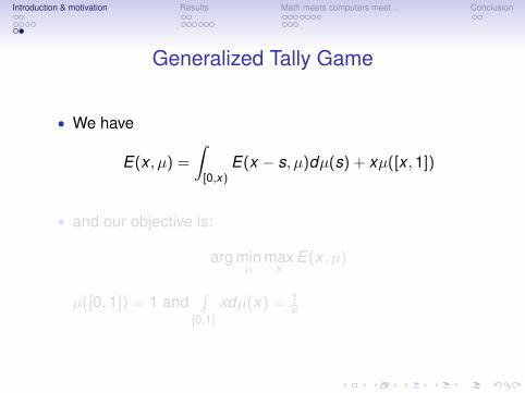
• We have
E(x , µ) =
∫[0,x)
E(x − s, µ)dµ(s) + xµ([x ,1])
• and our objective is:
arg minµ
maxx
E(x , µ)
µ([0,1]) = 1 and∫
[0,1]xdµ(x) = 1
2
Introduction & motivation Results Math meets computers meet... Conclusion
Generalized Tally Game
• We have
E(x , µ) =
∫[0,x)
E(x − s, µ)dµ(s) + xµ([x ,1])
• and our objective is:
arg minµ
maxx
E(x , µ)
µ([0,1]) = 1 and∫
[0,1]xdµ(x) = 1
2

Introduction & motivation Results Math meets computers meet... Conclusion
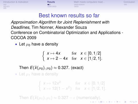
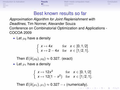
Best known results so farApproximation Algorithm for Joint Replenishment withDeadlines, Tim Nonner, Alexander SouzaConference on Combinatorial Optimization and Applications -COCOA 2009• Let µ0 have a density{
x 7→ 4x for x ∈ [0,1/2]x 7→ 2− 4x for x ∈ [1/2,1].
Then E(x(µ0), µ0) ≈ 0.327. (exact)• Let µ1 have a density{
x 7→ 12x2 for x ∈ [0,1/2]x 7→ 12(1− x2) for x ∈ [1/2,1].
Then E(x(µ1), µ1) ≈ 0.327− ε (numerically).
Introduction & motivation Results Math meets computers meet... Conclusion
Best known results so farApproximation Algorithm for Joint Replenishment withDeadlines, Tim Nonner, Alexander SouzaConference on Combinatorial Optimization and Applications -COCOA 2009• Let µ0 have a density{
x 7→ 4x for x ∈ [0,1/2]x 7→ 2− 4x for x ∈ [1/2,1].
Then E(x(µ0), µ0) ≈ 0.327. (exact)• Let µ1 have a density{
x 7→ 12x2 for x ∈ [0,1/2]x 7→ 12(1− x2) for x ∈ [1/2,1].
Then E(x(µ1), µ1) ≈ 0.327− ε (numerically).
Introduction & motivation Results Math meets computers meet... Conclusion
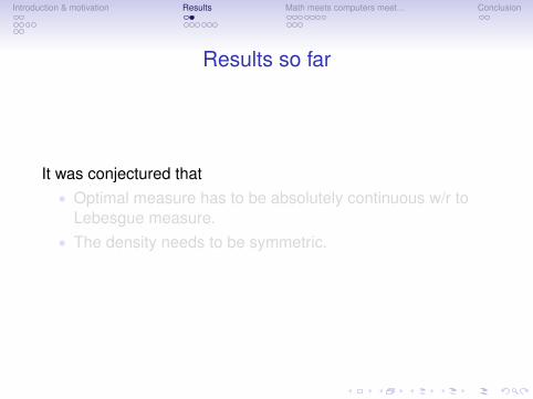
Results so far
It was conjectured that• Optimal measure has to be absolutely continuous w/r to
Lebesgue measure.• The density needs to be symmetric.

Introduction & motivation Results Math meets computers meet... Conclusion
Results so far
It was conjectured that• Optimal measure has to be absolutely continuous w/r to
Lebesgue measure.• The density needs to be symmetric.
Introduction & motivation Results Math meets computers meet... Conclusion
Results so far
It was conjectured that• Optimal measure has to be absolutely continuous w/r to
Lebesgue measure.• The density needs to be symmetric.

Introduction & motivation Results Math meets computers meet... Conclusion
Growth of x 7→ E(x , µ) bounded by 1
The analytic approach:
LemmaLet µ ∈M and h(x) be a positive, measurable function, soh(x) ≥ 0. Define H : [0,∞)→ R by H(x) := h(x) + H ∗ µ(x);Then H is a positive function.
• write G(x) = x − E(x) = xµ([0, x))− E ∗ µ(x);• then G(x) =
∫[0,x) ydµ(y) + G ∗ µ(x), so G ≥ 0.
• Now put Hy (x) = G(x + y)−G(x) = y + E(x)− E(x + y).• Then Hy (x) =
∫[x ,x+y)(G(x + y − s) + s)dµ(s) + Hy ∗ µ(x);
• Conclusion: E(x + y) ≤ E(x) + y .

Introduction & motivation Results Math meets computers meet... Conclusion
Existence and left-continuity of x 7→ E(x , µ)The series of convolutions approach:
given g, write g ∗ µ(x) =∫[0,x) g(x − z)dµ(z);
E(x , µ) = f (x) + E ∗ µ(x)
= f (x) + f ∗ µ(x) + (E ∗ µ) ∗ µ(x)
= f (x) + f ∗ µ(x) + (f ∗ µ) ∗ µ(x) + · · ·
= f (x) +∞∑
j=1
f (∗µ)j(x)
LemmaIf g is left-continuous then g ∗ µ is left-continuous.
• f is left-cs, so f ∗ µ, f (∗µ)2, f (∗µ)3 . . . are all left-cs;• just need to show that the higher terms are small:• f (∗µ)k (x) =
∫0≤
∑zi<x f (x − (z1 + · · ·+ zk ))dµk (z1, . . . , zk );
• µk (∑
zi < x) is exponentially small, by large deviations.

Introduction & motivation Results Math meets computers meet... Conclusion
We know now that E(x + y) ≤ E(x) + y and E isleft-continuous.
LemmaThe maximum of x 7→ E(x , µ) is realised.
Suppose µn → µ. How does fn(x) := xµn([x ,1]) behave?.• lim supε→0 limµn→µ fn(x − ε) = f (x , µ).• OR, for all ε > 0, there exists δ0 < y , and if 0 < δ < δ0,
there is N, breathe deeply, if n ≥ N, for all α ∈ [δ, δ0]
|f (y)− fn(y − α)| ≤ ε.
• “left-convergence”

Introduction & motivation Results Math meets computers meet... Conclusion
LemmaIf gn left-converges to g and µn → µ then gn ∗ µn left-convergesto g ∗ µ.
TheoremIf µn converges to µ then E(·, µn) left-converges to E(·, µ).
By Lemma, left-convergence of fn(∗µn)j → f (∗µ)j holds for all j .
TheoremIf µn converges to µ then E(·, µn) left-converges to E(·, µ).

Introduction & motivation Results Math meets computers meet... Conclusion
Theoremµ 7→ maxx E(x , µ) is continuous, for probability measures µsupported on [0,1].
• By left-convergence, given ε > 0, for large n there is apoint xn such that |E(xn, µn)− E(x , µ)| < ε;
• so lim maxy E(y , µn) ≥ maxy E(y , µ);• Let xn maximise E(·, µn) and xn → x (subsequence).
E(xn − ε, µn) ≥ E(xn, µn)− ε. Take limε→0 limn→∞:• Get E(x , µ) ≥ lim E(xn, µn), as required.
Corollary (Optimal measure exists)
There exists a measure µ0 minimising maxx E(x , µ) over allprobability measures with support on [0,1] and expected value1/2.

Introduction & motivation Results Math meets computers meet... Conclusion
Local search
We consider discrete measures supported on points kn ,
k = 1, . . . ,n.We start with a measure µ with µ([0,1]) = 1 and E(µ) = 1
2 .1 We chose 0 < k1 < k2 < k3 ≤ n at random.2 We construct a unique measure ν supported on {k1
n ,k2n ,
k3n }
with ν([0,1]) = 0 and E(ν) = 0.3 We try to find t such that µ+ t · ν is a measure (no negative
values allowed!) and that supx
E(x , µ+ t · ν) < supx
E(x , µ).
4 If we succeed: we replace µ with µ+ t · ν.Rinse & repeat

Introduction & motivation Results Math meets computers meet... Conclusion
Local Search in action
0.33162
0.0 0.2 0.4 0.6 0.8 1.00.0
0.2
0.4
0.6
0.8
1.0
0.0 0.2 0.4 0.6 0.8 1.0
.01
.02
.03
Figure: Starting measure - "two parabolas"

Introduction & motivation Results Math meets computers meet... Conclusion
Local Search in action
0.329389
0.0 0.2 0.4 0.6 0.8 1.00.0
0.2
0.4
0.6
0.8
1.0
0.0 0.2 0.4 0.6 0.8 1.0
.01
.02
.03
Figure: After 5 steps of optimization

Introduction & motivation Results Math meets computers meet... Conclusion
Local Search in action
0.305838
0.0 0.2 0.4 0.6 0.8 1.00.0
0.2
0.4
0.6
0.8
1.0
0.0 0.2 0.4 0.6 0.8 1.0
.01
.02
.03
Figure: After 15 steps of optimization

Introduction & motivation Results Math meets computers meet... Conclusion
Local Search in action
0.297408
0.0 0.2 0.4 0.6 0.8 1.00.0
0.2
0.4
0.6
0.8
1.0
0.0 0.2 0.4 0.6 0.8 1.0
.01
.02
.03
Figure: After ∼ 100 steps of optimization

Introduction & motivation Results Math meets computers meet... Conclusion
Local Search in action
0.290546
0.0 0.2 0.4 0.6 0.8 1.00.0
0.2
0.4
0.6
0.8
1.0
0.0 0.2 0.4 0.6 0.8 1.0
.01
.02
.03
Figure: After ∼ 200 steps of optimization

Introduction & motivation Results Math meets computers meet... Conclusion
Local Search in action
0.288311
0.0 0.2 0.4 0.6 0.8 1.00.0
0.2
0.4
0.6
0.8
1.0
0.0 0.2 0.4 0.6 0.8 1.0
.01
.02
.03
Figure: After� 1000 steps of optimization
Introduction & motivation Results Math meets computers meet... Conclusion
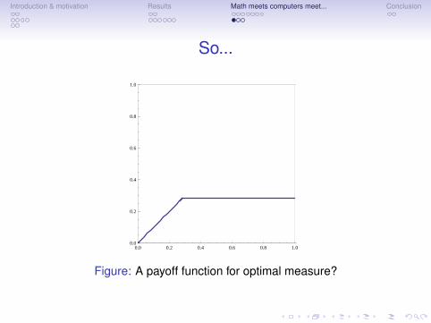
So...
0.0 0.2 0.4 0.6 0.8 1.00.0
0.2
0.4
0.6
0.8
1.0
Figure: A payoff function for optimal measure?

Introduction & motivation Results Math meets computers meet... Conclusion
Indeed
A measure with density function
g(x) =
0 for x ∈ [0,h)1x for x ∈ [h,2h)1x
(1− ln
( xh − 1
))for x ∈ [2h,3h)
Li2(2− xh )+ln( x
h−2) ln( xh−1)−ln( x
h−1)+π212 +1
x for x ∈ [3h,4h). . .
has expected payoff function
min(x ,h).

Introduction & motivation Results Math meets computers meet... Conclusion
Some calculations
• Recall:
min(x ,h) =
∫[0,x)
min(x − s,h)dµ(s) + xµ((x ,+∞))
So µ|(0,h) = 0 and
h =
∫(x−h,x)
(x − s)dµ(s) + hµ([0, x − h) + xµ((x ,+∞)).
• Differentiating by x we get
xg(x) = µ([x − h,+∞))
which we recursively solve.

Introduction & motivation Results Math meets computers meet... Conclusion
Conjecture
The functionmin(x ,h0),
where h0 = 0.28166214011768503‘ is the optimal payofffunction in Generalized Tally Game.
0.28166214011768503‘� 0.327− ε

Introduction & motivation Results Math meets computers meet... Conclusion
What next?
Algorithms & applications
we are doneHsort of L
Mathematicsoptimality
properties
how and why?


![[Slides] Crowdsourcing Pareto-Optimal Object Finding By Pairwise Comparisons](https://img.pdfslide.us/doc/110x75/58f373131a28ab6b518b4621/slides-crowdsourcing-pareto-optimal-object-finding-by-pairwise-comparisons.jpg)