Finding the k Shortest Paths

David Eppstein∗

March 31, 1997

Abstract

We give algorithms for finding the k shortest paths (not required to be simple) connecting apair of vertices in a digraph. Our algorithms output an implicit representation of these paths in adigraph with n vertices and m edges, in time O(m+ n log n+ k). We can also find the k shortestpaths from a given source s to each vertex in the graph, in total time O(m+n log n+ kn). We de-scribe applications to dynamic programming problems including the knapsack problem, sequencealignment, maximum inscribed polygons, and genealogical relationship discovery.

1 Introduction

We consider a long-studied generalization of the shortest path problem, in which not one but severalshort paths must be produced. The k shortest paths problem is to list the k paths connecting a givensource-destination pair in the digraph with minimum total length. Our techniques also apply to theproblem of listing all paths shorter than some given threshhold length. In the version of these problemsstudied here, cycles of repeated vertices are allowed. We first present a basic version of our algorithm,which is simple enough to be suitable for practical implementation while losing only a logarithmicfactor in time complexity. We then show how to achieve optimal time (constant time per path once ashortest path tree has been computed) by applying Frederickson’s [26] algorithm for finding the min-imum k elements in a heap-ordered tree.

1.1 Applications

The applications of shortest path computations are too numerous to cite in detail. They include situa-tions in which an actual path is the desired output, such as robot motion planning, highway and powerline engineering, and network connection routing. They include problems of scheduling such as criti-cal path computation in PERT charts. Many optimization problems solved by dynamic programmingor more complicated matrix searching techniques, such as the knapsack problem, sequence alignmentin molecular biology, construction of optimal inscribed polygons, and length-limited Huffman coding,can be expressed as shortest path problems.

∗Department of Information and Computer Science, University of California, Irvine, CA 92697-3425, eppstein@ics.uci.edu, http://www.ics.uci.edu/∼eppstein/. Supported in part by NSF grant CCR-9258355 and by matching funds from XeroxCorp.

1

Methods for finding k shortest paths have been applied to many of these applications, for severalreasons.

• Additional constraints. One may wish to find a path that satisfies certain constraints beyondhaving a small length, but those other constraints may be ill-defined or hard to optimize. Forinstance, in power transmission route selection [18], a power line should connect its endpointsreasonably directly, but there may be more or less community support for one option or another.A typical solution is to compute several short paths and then choose among them by consideringthe other criteria. We recently implemented a similar technique as a heuristic for the NP-hardproblem of, given a graph with colored edges, finding a shortest path using each color at mostonce [20]. This type of application is the main motivation cited by Dreyfus [17] and Lawler [39]for k shortest path computations.

• Model evaluation. Paths may be used to model problems that have known solutions, indepen-dent of the path formulation; for instance, in a k-shortest-path model of automatic translationbetween natural languages [30], a correct translation can be found by a human expert. By listingpaths until this known solution appears, one can determine how well the model fits the problem,in terms of the number of incorrect paths seen before the correct path. This information can beused to tune the model as well as to determine the number of paths that need to be generatedwhen applying additional constraints to search for the correct solution.

• Sensitivity analysis. By computing more than one shortest path, one can determine how sen-sitive the optimal solution is to variation of the problem’s parameters. In biological sequencealignment, for example, one typically wishes to see several “good” alignments rather than oneoptimal alignment; by comparing these several alignments, biologists can determine which por-tions of an alignment are most essential [8,64]. This problem can be reduced to finding severalshortest paths in a grid graph.

• Generation of alternatives. It may be useful to examine not just the optimal solution to a prob-lem, but a larger class of solutions, to gain a better understanding of the problem. For example,the states of a complex system might be represented as a finite state machine, essentially justa graph, with different probabilities on each state transition edge. In such a model, one wouldlikely want to know not just the chain of events most likely to lead to a failure state, but rather allchains having a failure probability over some threshhold. Taking the logarithms of the transitionprobabilities transforms this problem into one of finding all paths shorter than a given length.

We later discuss in more detail some of the dynamic programming applications listed above, andshow how to find the k best solutions to these problems by using our shortest path algorithms. Aswell as improving previous solutions to the general k shortest paths problem, our results improve morespecialized algorithms for finding length-bounded paths in the grid graphs arising in sequence align-ment [8] and for finding the k best solutions to the knapsack problem [15].

2

1.2 New Results

We prove the following results. In all cases we assume we are given a digraph in which each edge hasa non-negative length. We allow the digraph to contain self-loops and multiple edges. In each casethe paths are output in an implicit representation from which simple properties such as the length areavailable in constant time per path. We may explicitly list the edges in any path in time proportionalto the number of edges.

• We find the k shortest paths (allowing cycles) connecting a given pair of vertices in a digraph,in time O(m+ n log n+ k).

• We find the k shortest paths from a given source in a digraph to each other vertex, in time O(m+n log n+ kn).

We can also solve the similar problem of finding all paths shorter than a given length, with the sametime bounds. The same techniques apply to digraphs with negative edge lengths but no negative cycles,but the time bounds above should be modified to include the time to compute a single source shortestpath tree in such networks, O(mn) [6,23] or O(mn1/2 log N)where all edge lengths are integers and Nis the absolute value of the most negative edge length [29]. For a directed acyclic graph (DAG), with orwithout negative edge lengths, shortest path trees can be constructed in linear time and the O(n log n)term above can be omitted. The related problem of finding the k longest paths in a DAG [4] can betransformed to a shortest path problem simply by negating all edge lengths; we can therefore also solveit in the same time bounds.

1.3 Related Work

Many papers study algorithms for k shortest paths [3,5,7,9,13,14,17,24,31,32,34,35,37–41,43–45,47, 50, 51, 56–60, 63, 65–69]. Dreyfus [17] and Yen [69] cite several additional papers on the subjectgoing back as far as 1957.

One must distinguish several common variations of the problem. In many of the papers cited above,the paths are restricted to be simple, i.e. no vertex can be repeated. This has advantages in some appli-cations, but as our results show this restriction seems to make the problem significantly harder. Severalpapers [3, 13, 17, 24, 41, 42, 58, 59] consider the version of the k shortest paths problem in which re-peated vertices are allowed, and it is this version that we also study. Of course, for the DAGs that arisein many of the applications described above including scheduling and dynamic programming, no pathcan have a repeated vertex and the two versions of the problem become equivalent. Note also that inthe application described earlier of listing the most likely failure paths of a system modelled by a finitestate machine, it is the version studied here rather than the more common simple path version that onewants to solve.

One can also make a restriction that the paths found be edge disjoint or vertex disjoint [61], orinclude capacities on the edges [10–12, 49], however such changes turn the problem into one moreclosely related to network flow.

Fox [24] gives a method for the k shortest path problem based on Dijkstra’s algorithm which withmore recent improvements in priority queue data structures [27] takes time O(m+kn log n); this seems

3

to be the best previously known k-shortest-paths algorithm. Dreyfus [17] mentions the version of theproblem in which we must find paths from one source to each other vertex in the graph, and describesa simple O(kn2) time dynamic programming solution to this problem. For the k shortest simple pathsproblem, the best known bound is O(k(m+n log n)) in undirected graphs [35] or O(kn(m+n log n))in directed graphs [39, again including more recent improvements in Dijkstra’s algorithm]. Thus allprevious algorithms took time O(n log n) or more per path. We improve this to constant time per path.

A similar problem to the one studied here is that of finding the k minimum weight spanning treesin a graph. Recent algorithms for this problem [21, 22, 25] reduce it to finding the k minimum weightnodes in a heap-ordered tree, defined using the best swap in a sequence of graphs. Heap-ordered treeselection has also been used to find the smallest interpoint distances or the nearest neighbors in geomet-ric point sets [16]. We apply a similar tree selection technique to the k shortest path problem, howeverthe reduction of k shortest paths to heap ordered trees is very different from the constructions in theseother problems.

2 The Basic Algorithm

Finding the k shortest paths between two terminals s and t has been a difficult enough problem to war-rant much research. In contrast, the similar problem of finding paths with only one terminal s, endinganywhere in the graph, is much easier: one can simply use breadth first search. Maintain a priorityqueue of paths, initially containing the single zero-edge path from s to itself; then repeatedly removethe shortest path from the priority queue, add it to the list of output paths, and add all one-edge exten-sions of that path to the priority queue. If the graph has bounded degree d, a breadth first search froms until k paths are found takes time O(dk+ k log k); note that this bound does not depend in any wayon the overall size of the graph. If the paths need not be output in order by length, Frederickson’s heapselection algorithm [26] can be used to speed this up to O(dk).

The main idea of our k shortest paths algorithm, then, is to translate the problem from one with twoterminals, sand t , to a problem with only one terminal. One can find paths from s to t simply by findingpaths from s to any other vertex and concatenating a shortest path from that vertex to t . However wecannot simply apply this idea directly, for several reasons: (1) There is no obvious relation between theordering of the paths from s to other vertices, and of the corresponding paths from s to t . (2) Each pathfrom s to t may be represented in many ways as a path from s to some vertex followed by a shortestpath from that vertex to t . (3) Our input graph may not have bounded degree.

In outline, we deal with problem (1) by using a potential function to modify the edge lengths in thegraph so that the length of any shortest path to t is zero; therefore concatenating such paths to pathsfrom s will preserve the ordering of the path lengths. We deal with problem (2) by only consideringpaths from s in which the last edge is not in a fixed shortest path tree to t ; this leads to the implicitrepresentation we use to represent each path in constant space. (Similar ideas to these appear alsoin [46].) However this solution gives rise to a fourth problem: (4) We do not wish to spend much timesearching edges of the shortest path tree, as this time can not be charged against newly found s-t paths.

The heart of our algorithm is the solution to problems (3) and (4). Our idea is to construct a bi-nary heap for each vertex, listing the edges that are not part of the shortest path tree and that can bereached from that vertex by shortest-path-tree edges. In order to save time and space, we use persis-

4

tence techniques to allow these heaps to share common structures with each other. In the basic versionof the algorithm, this collection of heaps forms a bounded-degree graph having O(m+ n log n) ver-tices. Later we show how to improve the time and space bounds of this part of the algorithm using treedecomposition techniques of Frederickson [25].

2.1 Preliminaries

We assume throughout that our input graph G has n vertices and m edges. We allow self-loops andmultiple edges so m may be larger than

(n2

). The length of an edge e is denoted `(e). By extension

we can define the length `(p) for any path in G to be the sum of its edge lengths. The distance d(s, t)for a given pair of vertices is the length of the shortest path starting at s and ending at t ; with the as-sumption of no negative cycles this is well defined. Note that d(s, t) may be unequal to d(t, s). Thetwo endpoints of a directed edge e are denoted tail(e) and head(e); the edge is directed from tail(e) tohead(e).

For our purposes, a heap is a binary tree in which vertices have weights, satisfying the restrictionthat the weight of any vertex is less than or equal to the minimum weight of its children. We will notalways care whether the tree is balanced (and in some circumstances we will allow trees with infinitedepth). More generally, a D-heap is a degree-D tree with the same weight-ordering property; thus theusual heaps above are 2-heaps. As is well known (e.g. see [62]), any set of values can be placed intoa balanced heap by the heapify operation in linear time. In a balanced heap, any new element can beinserted in logarithmic time. We can list the elements of a heap in order by weight, taking logarithmictime to generate each element, simply by using breadth first search.

2.2 Implicit Representation of Paths

As discussed earlier, our algorithm does not output each path it finds explicitly as a sequence of edges;instead it uses an implicit representation, described in this section.

The i th shortest path in a digraph may haveÄ(ni) edges, so the best time we could hope for in anexplicit listing of shortest paths would be O(k2n). Our time bounds are faster than this, so we mustuse an implicit representation for the paths. However our representation is not a serious obstacle touse of our algorithm: we can list the edges of any path we output in time proportional to the number ofedges, and simple properties (such as the length) are available in constant time. Similar implicit rep-resentations have previously been used for related problems such as the k minimum weight spanningtrees [21, 22, 25]. Further, previous papers on the k shortest path problem give time bounds omittingthe O(k2n) term above, and so these papers must tacitly or not be using an implicit representation.

Our representation is similar in spirit to those used for the k minimum weight spanning trees prob-lem: for that problem, each successive tree differs from a previously listed tree by a swap, the insertionof one edge and removal of another edge. The implicit representation consists of a pointer to the pre-vious tree, and a description of the swap. For the shortest path problem, each successive path will turnout to differ from a previously listed path by the inclusion of a single edge not part of a shortest pathtree, and appropriate adjustments in the portion of the path that involves shortest path tree edges. Ourimplicit representation consists of a pointer to the previous path, and a description of the newly addededge.

5

s

t11

12

109

13

818

7

15

14202

27

15 20

14

25

0111937

7233342

22365655

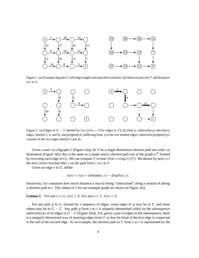
Figure 1. (a) Example digraph G with edge lengths and specified terminals; (b) Shortest path tree T and distancesto t in G.

s

t

3

4

10 6

1

9

s

t

3

4

9

Figure 2. (a) Edges in G − T labeled by δ(e) (δ(e) = 0 for edges in T); (b) Path p, sidetracks(p) (the heavyedges, labeled 3, 4, and 9), and prefpath(p) (differing from p in the two dashed edges; sidetracks(prefpath(p))consists of the two edges labeled 3 and 4).

Given s and t in a digraph G (Figure 1(a)), let T be a single-destination shortest path tree with t asdestination (Figure 1(b); this is the same as a single source shortest path tree in the graph GR formedby reversing each edge of G). We can compute T in time O(m+n log n) [27]. We denote by nextT (v)the next vertex reached after v on the path from v to t in T .

Given an edge e in G, define

δ(e) = `(e)+ d(head(e), t)− d(tail(e), t).

Intuitively, δ(e) measures how much distance is lost by being “sidetracked” along e instead of takinga shortest path to t . The values of δ for our example graph are shown in Figure 2(a).

Lemma 1. For any e∈ G, δ(e) ≥ 0. For any e∈ T , δ(e) = 0.

For any path p in G, formed by a sequence of edges, some edges of p may be in T , and someothers may be in G − T . Any path p from s to t is uniquely determined solely by the subsequencesidetracks(p) of its edges in G− T (Figure 2(b)). For, given a pair of edges in the subsequence, thereis a uniquely determined way of inserting edges from T so that the head of the first edge is connectedto the tail of the second edge. As an example, the shortest path in T from s to t is represented by the

6

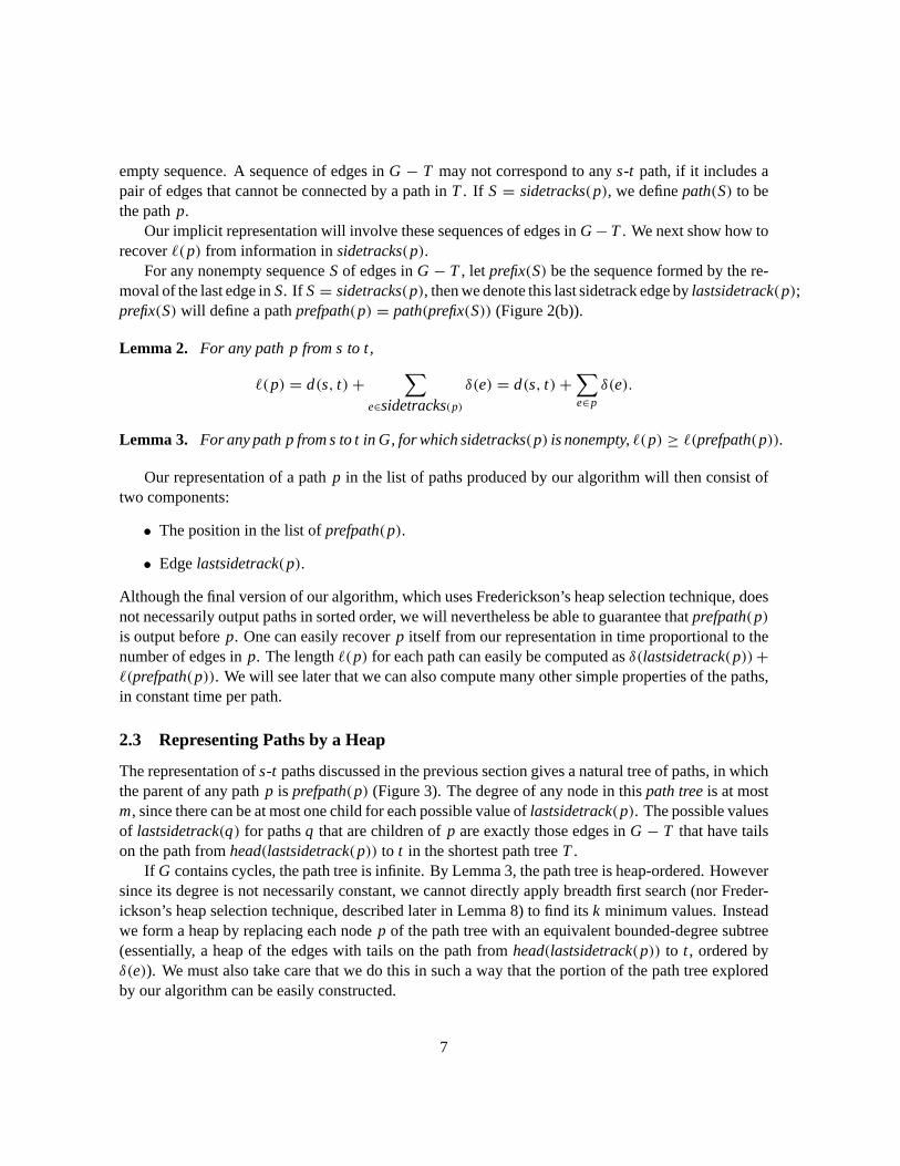
empty sequence. A sequence of edges in G − T may not correspond to any s-t path, if it includes apair of edges that cannot be connected by a path in T . If S= sidetracks(p), we define path(S) to bethe path p.

Our implicit representation will involve these sequences of edges in G−T . We next show how torecover `(p) from information in sidetracks(p).

For any nonempty sequence Sof edges in G− T , let prefix(S) be the sequence formed by the re-moval of the last edge in S. If S= sidetracks(p), then we denote this last sidetrack edge by lastsidetrack(p);prefix(S) will define a path prefpath(p) = path(prefix(S)) (Figure 2(b)).

Lemma 2. For any path p from s to t ,

`(p) = d(s, t)+∑

e∈sidetracks(p)δ(e) = d(s, t)+

∑e∈p

δ(e).

Lemma 3. For any path p from s to t in G, for which sidetracks(p) is nonempty, `(p) ≥ `(prefpath(p)).

Our representation of a path p in the list of paths produced by our algorithm will then consist oftwo components:

• The position in the list of prefpath(p).

• Edge lastsidetrack(p).

Although the final version of our algorithm, which uses Frederickson’s heap selection technique, doesnot necessarily output paths in sorted order, we will nevertheless be able to guarantee that prefpath(p)is output before p. One can easily recover p itself from our representation in time proportional to thenumber of edges in p. The length `(p) for each path can easily be computed as δ(lastsidetrack(p))+`(prefpath(p)). We will see later that we can also compute many other simple properties of the paths,in constant time per path.

2.3 Representing Paths by a Heap

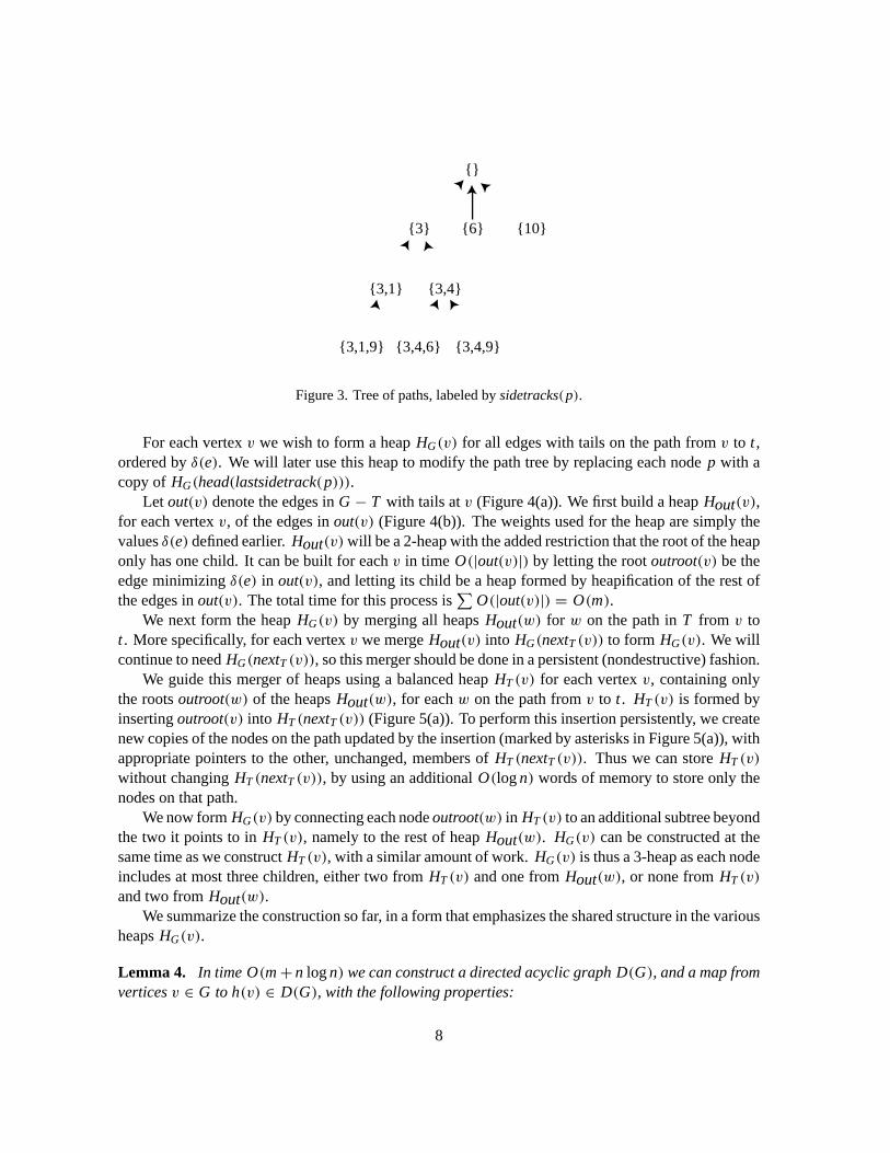
The representation of s-t paths discussed in the previous section gives a natural tree of paths, in whichthe parent of any path p is prefpath(p) (Figure 3). The degree of any node in this path tree is at mostm, since there can be at most one child for each possible value of lastsidetrack(p). The possible valuesof lastsidetrack(q) for paths q that are children of p are exactly those edges in G − T that have tailson the path from head(lastsidetrack(p)) to t in the shortest path tree T .

If G contains cycles, the path tree is infinite. By Lemma 3, the path tree is heap-ordered. Howeversince its degree is not necessarily constant, we cannot directly apply breadth first search (nor Freder-ickson’s heap selection technique, described later in Lemma 8) to find its k minimum values. Insteadwe form a heap by replacing each node p of the path tree with an equivalent bounded-degree subtree(essentially, a heap of the edges with tails on the path from head(lastsidetrack(p)) to t , ordered byδ(e)). We must also take care that we do this in such a way that the portion of the path tree exploredby our algorithm can be easily constructed.

7

{}

{3}

{3,1} {3,4}

{3,4,6} {3,4,9}

{6} {10}

{3,1,9}

Figure 3. Tree of paths, labeled by sidetracks(p).

For each vertex v we wish to form a heap HG(v) for all edges with tails on the path from v to t ,ordered by δ(e). We will later use this heap to modify the path tree by replacing each node p with acopy of HG(head(lastsidetrack(p))).

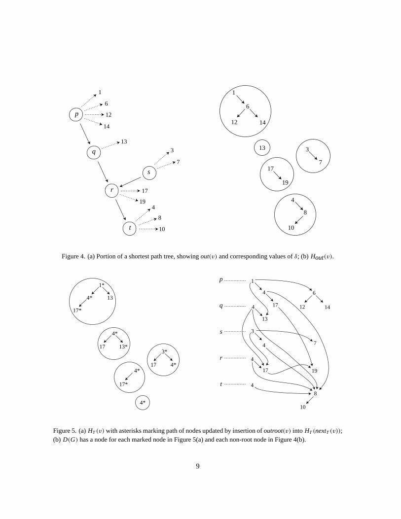
Let out(v) denote the edges in G− T with tails at v (Figure 4(a)). We first build a heap Hout(v),for each vertex v, of the edges in out(v) (Figure 4(b)). The weights used for the heap are simply thevalues δ(e) defined earlier. Hout(v)will be a 2-heap with the added restriction that the root of the heaponly has one child. It can be built for each v in time O(|out(v)|) by letting the root outroot(v) be theedge minimizing δ(e) in out(v), and letting its child be a heap formed by heapification of the rest ofthe edges in out(v). The total time for this process is

∑O(|out(v)|) = O(m).

We next form the heap HG(v) by merging all heaps Hout(w) for w on the path in T from v tot . More specifically, for each vertex v we merge Hout(v) into HG(nextT (v)) to form HG(v). We willcontinue to need HG(nextT (v)), so this merger should be done in a persistent (nondestructive) fashion.

We guide this merger of heaps using a balanced heap HT (v) for each vertex v, containing onlythe roots outroot(w) of the heaps Hout(w), for each w on the path from v to t . HT (v) is formed byinserting outroot(v) into HT (nextT (v)) (Figure 5(a)). To perform this insertion persistently, we createnew copies of the nodes on the path updated by the insertion (marked by asterisks in Figure 5(a)), withappropriate pointers to the other, unchanged, members of HT (nextT (v)). Thus we can store HT (v)

without changing HT (nextT (v)), by using an additional O(log n) words of memory to store only thenodes on that path.

We now form HG(v) by connecting each node outroot(w) in HT (v) to an additional subtree beyondthe two it points to in HT (v), namely to the rest of heap Hout(w). HG(v) can be constructed at thesame time as we construct HT (v), with a similar amount of work. HG(v) is thus a 3-heap as each nodeincludes at most three children, either two from HT (v) and one from Hout(w), or none from HT (v)

and two from Hout(w).We summarize the construction so far, in a form that emphasizes the shared structure in the various

heaps HG(v).

Lemma 4. In time O(m+n log n) we can construct a directed acyclic graph D(G), and a map fromvertices v ∈ G to h(v) ∈ D(G), with the following properties:

8

1

6

12

14

13

3

7

17

194

8

10

p

q

r

s

t

1

6

12 14

13 3

717

19

4

8

10

Figure 4. (a) Portion of a shortest path tree, showing out(v) and corresponding values of δ; (b) Hout(v).

4*

4*

17*

4*

13*17

17*

1*

134*

3*

4*17

p

q

r

s

t 4

4

17

17

3

4

4

13

1

4 6

12 14

7

19

8

10

Figure 5. (a) HT (v) with asterisks marking path of nodes updated by insertion of outroot(v) into HT (nextT (v));(b) D(G) has a node for each marked node in Figure 5(a) and each non-root node in Figure 4(b).

9

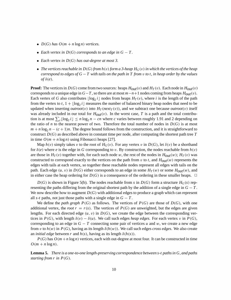
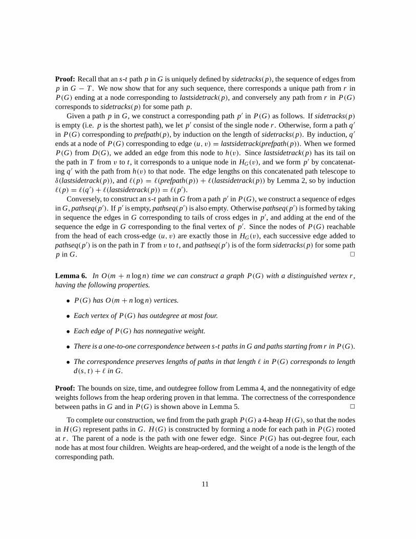
• D(G) has O(m+ n log n) vertices.

• Each vertex in D(G) corresponds to an edge in G− T .

• Each vertex in D(G) has out-degree at most 3.

• The vertices reachable in D(G) from h(v) form a 3-heap HG(v) in which the vertices of the heapcorrespond to edges of G−T with tails on the path in T from v to t , in heap order by the valuesof δ(e).

Proof: The vertices in D(G) come from two sources: heaps Hout(v) and HT (v). Each node in Hout(v)corresponds to a unique edge in G−T , so there are at most m−n+1 nodes coming from heaps Hout(v).Each vertex of G also contributes blog2 i c nodes from heaps HT (v), where i is the length of the pathfrom the vertex to t , 1+ blog2 i c measures the number of balanced binary heap nodes that need to beupdated when inserting outroot(v) into HT (nextT (v)), and we subtract one because outroot(v) itselfwas already included in our total for Hout(v). In the worst case, T is a path and the total contribu-tion is at most

∑i blog2 i c ≤ n log2 n− cn where c varies between roughly 1.91 and 2 depending on

the ratio of n to the nearest power of two. Therefore the total number of nodes in D(G) is at mostm+ n log2 n− (c+ 1)n. The degree bound follows from the construction, and it is straightforward toconstruct D(G) as described above in constant time per node, after computing the shortest path tree Tin time O(m+ n log n) using Fibonacci heaps [27].

Map h(v) simply takes v to the root of HG(v). For any vertex v in D(G), let δ(v) be a shorthandfor δ(e) where e is the edge in G corresponding to v. By construction, the nodes reachable from h(v)are those in HT (v) together with, for each such node w, the rest of the nodes in Hout(w); HT (v) wasconstructed to correspond exactly to the vertices on the path from v to t , and Hout(w) represents theedges with tails at each vertex, so together these reachable nodes represent all edges with tails on thepath. Each edge (u, v) in D(G) either corresponds to an edge in some HT (w) or some Hout(w), andin either case the heap ordering for D(G) is a consequence of the ordering in these smaller heaps. 2

D(G) is shown in Figure 5(b). The nodes reachable from s in D(G) form a structure HG(s) rep-resenting the paths differing from the original shortest path by the addition of a single edge in G− T .We now describe how to augment D(G)with additional edges to produce a graph which can representall s-t paths, not just those paths with a single edge in G− T .

We define the path graph P(G) as follows. The vertices of P(G) are those of D(G), with oneadditional vertex, the root r = r (s). The vertices of P(G) are unweighted, but the edges are givenlengths. For each directed edge (u, v) in D(G), we create the edge between the corresponding ver-tices in P(G), with length δ(v) − δ(u). We call such edges heap edges. For each vertex v in P(G),corresponding to an edge in G − T connecting some pair of vertices u and w, we create a new edgefrom v to h(w) in P(G), having as its length δ(h(w)). We call such edges cross edges. We also createan initial edge between r and h(s), having as its length δ(h(s)).

P(G) has O(m+n log n) vertices, each with out-degree at most four. It can be constructed in timeO(m+ n log n).

Lemma 5. There is a one-to-one length-preserving correspondence between s-t paths in G, and pathsstarting from r in P(G).

10

Proof: Recall that an s-t path p in G is uniquely defined by sidetracks(p), the sequence of edges fromp in G − T . We now show that for any such sequence, there corresponds a unique path from r inP(G) ending at a node corresponding to lastsidetrack(p), and conversely any path from r in P(G)corresponds to sidetracks(p) for some path p.

Given a path p in G, we construct a corresponding path p′ in P(G) as follows. If sidetracks(p)is empty (i.e. p is the shortest path), we let p′ consist of the single node r . Otherwise, form a path q′

in P(G) corresponding to prefpath(p), by induction on the length of sidetracks(p). By induction, q′

ends at a node of P(G) corresponding to edge (u, v) = lastsidetrack(prefpath(p)). When we formedP(G) from D(G), we added an edge from this node to h(v). Since lastsidetrack(p) has its tail onthe path in T from v to t , it corresponds to a unique node in HG(v), and we form p′ by concatenat-ing q′ with the path from h(v) to that node. The edge lengths on this concatenated path telescope toδ(lastsidetrack(p)), and `(p) = `(prefpath(p)) + `(lastsidetrack(p)) by Lemma 2, so by induction`(p) = `(q′)+ `(lastsidetrack(p)) = `(p′).

Conversely, to construct an s-t path in G from a path p′ in P(G), we construct a sequence of edgesin G, pathseq(p′). If p′ is empty, pathseq(p′) is also empty. Otherwise pathseq(p′) is formed by takingin sequence the edges in G corresponding to tails of cross edges in p′, and adding at the end of thesequence the edge in G corresponding to the final vertex of p′. Since the nodes of P(G) reachablefrom the head of each cross-edge (u, v) are exactly those in HG(v), each successive edge added topathseq(p′) is on the path in T from v to t , and pathseq(p′) is of the form sidetracks(p) for some pathp in G. 2

Lemma 6. In O(m + n log n) time we can construct a graph P(G) with a distinguished vertex r ,having the following properties.

• P(G) has O(m+ n log n) vertices.

• Each vertex of P(G) has outdegree at most four.

• Each edge of P(G) has nonnegative weight.

• There is a one-to-one correspondence between s-t paths in G and paths starting from r in P(G).

• The correspondence preserves lengths of paths in that length ` in P(G) corresponds to lengthd(s, t)+ ` in G.

Proof: The bounds on size, time, and outdegree follow from Lemma 4, and the nonnegativity of edgeweights follows from the heap ordering proven in that lemma. The correctness of the correspondencebetween paths in G and in P(G) is shown above in Lemma 5. 2

To complete our construction, we find from the path graph P(G) a 4-heap H(G), so that the nodesin H(G) represent paths in G. H(G) is constructed by forming a node for each path in P(G) rootedat r . The parent of a node is the path with one fewer edge. Since P(G) has out-degree four, eachnode has at most four children. Weights are heap-ordered, and the weight of a node is the length of thecorresponding path.

11

Lemma 7. H(G) is a 4-heap in which there is a one-to-one correspondence between nodes and s-tpaths in G, and in which the length of a path in G is d(s, t) plus the weight of the corresponding nodein H(G).

We note that, if an algorithm explores a connected region of O(k) nodes in H(G), it can representthe nodes in constant space each by assigning them numbers and indicating for each node its parentand the additional edge in the corresponding path of P(G). The children of a node are easy to findsimply by following appropriate out-edges in P(G), and the weight of a node is easy to compute fromthe weight of its parent. It is also easy to maintain along with this representation the correspondingimplicit representation of s-t paths in G.

2.4 Finding the k Shortest Paths

Theorem 1. In time O(m+ n log n) we can construct a data structure that will output the shortestpaths from s to t in a graph in order by weight, taking time O(log i ) to output the i th path.

Proof: We apply breadth first search to P(G), as described at the start of the section, and translate thesearch results to paths using the correspondence described above. 2

We next describe how to compute paths from s to all n vertices of the graph. In fact our constructionsolves more easily the reverse problem, of finding paths from each vertex to the destination t . Theconstruction of P(G) is as above, except that instead of adding a single root r (s) connected to h(s),we add a root r (v) for each vertex v ∈ G. The modification to P(G) takes O(n) time. Using themodified P(G), we can compute a heap Hv(G) of paths from each v to t , and compute the k smallestsuch paths in time O(k).

Theorem 2. Given a source vertex s in a digraph G, we can find in time O(m+ n log n+ kn log k)an implicit representation of the k shortest paths from s to each other vertex in G.

Proof: We apply the construction above to GR, with s as destination. We form the modified path graphP(GR), find for each vertex v a heap Hv(GR) of paths in GR from v to s, and apply breadth first searchto this heap. Each resulting path corresponds to a path from s to v in G. 2

3 Improved Space and Time

The basic algorithm described above takes time O(m+ n log n+ k log k), even if a shortest path treehas been given. If the graph is sparse, the n log n term makes this bound nonlinear. This term comesfrom two parts of our method, Dijkstra’s shortest path algorithm and the construction of P(G) from thetree of shortest paths. But for certain graphs, or with certain assumptions about edge lengths, shortestpaths can be computed more quickly than O(m+ n log n) [2,28,33,36], and in these cases we wouldlike to speed up our construction of P(G) to match these improvements. In other cases, k may be largeand the k log k term may dominate the time bound; again we would like to improve this nonlinear term.In this section we show how to reduce the time for our algorithm to O(m+n+k), assuming a shortestpath tree is given in the input. As a consequence we can also improve the space used by our algorithm.

12

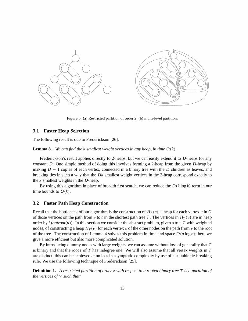
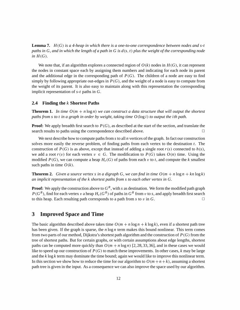
Figure 6. (a) Restricted partition of order 2; (b) multi-level partition.

3.1 Faster Heap Selection

The following result is due to Frederickson [26].

Lemma 8. We can find the k smallest weight vertices in any heap, in time O(k).

Frederickson’s result applies directly to 2-heaps, but we can easily extend it to D-heaps for anyconstant D. One simple method of doing this involves forming a 2-heap from the given D-heap bymaking D − 1 copies of each vertex, connected in a binary tree with the D children as leaves, andbreaking ties in such a way that the Dk smallest weight vertices in the 2-heap correspond exactly tothe k smallest weights in the D-heap.

By using this algorithm in place of breadth first search, we can reduce the O(k log k) term in ourtime bounds to O(k).

3.2 Faster Path Heap Construction

Recall that the bottleneck of our algorithm is the construction of HT (v), a heap for each vertex v in Gof those vertices on the path from v to t in the shortest path tree T . The vertices in HT (v) are in heaporder by δ(outroot(u)). In this section we consider the abstract problem, given a tree T with weightednodes, of constructing a heap HT (v) for each vertex v of the other nodes on the path from v to the rootof the tree. The construction of Lemma 4 solves this problem in time and space O(n log n); here wegive a more efficient but also more complicated solution.

By introducing dummy nodes with large weights, we can assume without loss of generality that Tis binary and that the root t of T has indegree one. We will also assume that all vertex weights in Tare distinct; this can be achieved at no loss in asymptotic complexity by use of a suitable tie-breakingrule. We use the following technique of Frederickson [25].

Definition 1. A restricted partition of order z with respect to a rooted binary tree T is a partition ofthe vertices of V such that:

13

1. Each set in the partition contains at most z vertices.

2. Each set in the partition induces a connected subtree of T .

3. For each set S in the partition, if S contains more than one vertex, then there are at most twotree edges having one endpoint in S.

4. No two sets can be combined and still satisfy the other conditions.

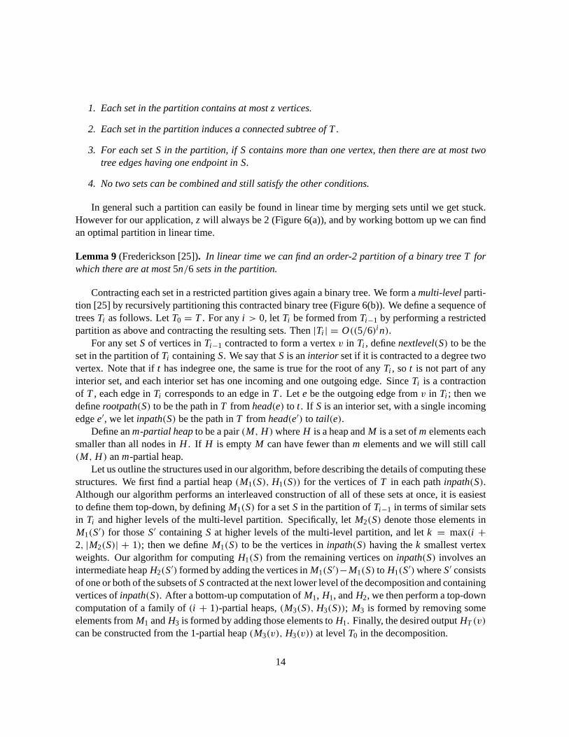
In general such a partition can easily be found in linear time by merging sets until we get stuck.However for our application, z will always be 2 (Figure 6(a)), and by working bottom up we can findan optimal partition in linear time.

Lemma 9 (Frederickson [25]). In linear time we can find an order-2 partition of a binary tree T forwhich there are at most 5n/6 sets in the partition.

Contracting each set in a restricted partition gives again a binary tree. We form a multi-level parti-tion [25] by recursively partitioning this contracted binary tree (Figure 6(b)). We define a sequence oftrees Ti as follows. Let T0 = T . For any i > 0, let Ti be formed from Ti−1 by performing a restrictedpartition as above and contracting the resulting sets. Then |Ti | = O((5/6)i n).

For any set S of vertices in Ti−1 contracted to form a vertex v in Ti , define nextlevel(S) to be theset in the partition of Ti containing S. We say that S is an interior set if it is contracted to a degree twovertex. Note that if t has indegree one, the same is true for the root of any Ti , so t is not part of anyinterior set, and each interior set has one incoming and one outgoing edge. Since Ti is a contractionof T , each edge in Ti corresponds to an edge in T . Let e be the outgoing edge from v in Ti ; then wedefine rootpath(S) to be the path in T from head(e) to t . If S is an interior set, with a single incomingedge e′, we let inpath(S) be the path in T from head(e′) to tail(e).

Define an m-partial heap to be a pair (M, H)where H is a heap and M is a set of m elements eachsmaller than all nodes in H . If H is empty M can have fewer than m elements and we will still call(M, H) an m-partial heap.

Let us outline the structures used in our algorithm, before describing the details of computing thesestructures. We first find a partial heap (M1(S), H1(S)) for the vertices of T in each path inpath(S).Although our algorithm performs an interleaved construction of all of these sets at once, it is easiestto define them top-down, by defining M1(S) for a set S in the partition of Ti−1 in terms of similar setsin Ti and higher levels of the multi-level partition. Specifically, let M2(S) denote those elements inM1(S′) for those S′ containing S at higher levels of the multi-level partition, and let k = max(i +2, |M2(S)| + 1); then we define M1(S) to be the vertices in inpath(S) having the k smallest vertexweights. Our algorithm for computing H1(S) from the remaining vertices on inpath(S) involves anintermediate heap H2(S′) formed by adding the vertices in M1(S′)−M1(S) to H1(S′)where S′ consistsof one or both of the subsets of Scontracted at the next lower level of the decomposition and containingvertices of inpath(S). After a bottom-up computation of M1, H1, and H2, we then perform a top-downcomputation of a family of (i + 1)-partial heaps, (M3(S), H3(S)); M3 is formed by removing someelements from M1 and H3 is formed by adding those elements to H1. Finally, the desired output HT (v)

can be constructed from the 1-partial heap (M3(v), H3(v)) at level T0 in the decomposition.

14

Before describing our algorithms, let us bound a quantity useful in their analysis. Let mi denotethe sum of |M1(S)| over sets Scontracted in Ti .

Lemma 10. For each i , mi = O(i |Ti |).

Proof: By the definition of M1(S) above,

mi =∑

S

max(i + 2, |M2(S)| + 1) ≤∑

S

|M2(S)| + i + 2 ≤ (i + 2)|Ti | +∑

S

|M2(S)|.

All sets M2(S) appearing in this sum are disjoint, and all are included in mi+1, so we can simplify thisformula to

mi ≤ (i + 2)|Ti | +mi+1 ≤∑j≥i

( j + 2)|Tj | ≤∑j≥i

( j + 2)(5

6

) j−i |Ti | = O(i |Ti |).

2

We use the following data structure to compute the sets M1(S) (which, recall, are sets of low-weightvertices on inpath(S)) . For each interior set S, we form a priority queue Q(S), from which we canretrieve the smallest weight vertex on inpath(S) not yet in M1(S). This data structure is very simple:if only one of the two subsets forming Scontains vertices on inpath(S), we simply copy the minimum-weight vertex on that subset’s priority queue, and otherwise we compare the minimum-weight verticesin each subset’s priority queue and select the smaller of the two weights. If one of the two subsets’priority queue values change, this structure can be updated simply by repeating this comparison.

We start by setting all the sets M1(S) to be empty, then progress top-down through the multi-leveldecomposition, testing for each set Sin each tree Ti (in decreasing order of i ) whether we have alreadyadded enough members to M1(S). If not, we add elements one at a time, until there are enough to satisfythe definition above of |M1(S)|. Whenever we add an element to M1(S) we add the same element toM1(S′) for each lower level subset S′ to which it also belongs. An element is added by removing itfrom Q(S) and from the priority queues of the sets at each lower level. We then update the queuesbottom up, recomputing the head of each queue and inserting it in the queue at the next level.

Lemma 11. The amount of time to compute M1(S) for all sets S in the multi-level partition, as de-scribed above, is O(n).

Proof: By Lemma 10, the number of operations in priority queues for subsets of Ti is O(i |Ti |). So thetotal time is

∑O(i |Ti |) = O(n

∑i (5/6)i ) = O(n). 2

We next describe how to compute the heaps H1(S) for the vertices on inpath(S) that have not beenchosen as part of M1(S). For this stage we work bottom up. Recall that Scorresponds to one or two ver-tices of Ti ; each vertex corresponds to a set S′ contracted at a previous level of the multi-level partition.For each such S′ along the path in Swe will have already formed the partial heap (M1(S′), H1(S′)). Welet H2(S′) be a heap formed by adding the vertices in M1(S′)−M1(S) to H1(S′). Since M1(S′)−M1(S)consists of at least one vertex (because of the requirement that |M1(S′)| ≥ |M1(S)| + 1), we can formH2(S′) as a 2-heap in which the root has degree one.

15

If Sconsists of a single vertex we then let H1(S) = H2(S′); otherwise we form H1(S) by combin-ing the two heaps H2(S′) for its two children. The time is constant per set Sor linear overall.

We next compute another collection of partial heaps (M3(S), H3(S)) of vertices in rootpath(S)for each set S contracted at some level of the tree. If S is a set contracted to a vertex in Ti , we let(M3(S), H3(S)) be an i + 1-partial heap. In this phase of the algorithm, we work top down. For eachset S, consisting of a collection of vertices in Ti−1, we use (M3(S), H3(S)) to compute for each vertexS′ the partial heap (M3(S′), H3(S′)).

If Sconsists of a single set S′, or if S′ is the parent of the two vertices in S, we let M3(S′) be formedby removing the minimum weight element from M3(S) and we let H3(S′) be formed by adding thatminimum weight element as a new root to H3(S).

In the remaining case, if S′ and parent(S′) are both in S, we form M3(S′) by taking the i + 1minimum values in M1(parent(S′)) ∪ M3(parent(S′)). The remaining values in M1(parent(S′)) ∪M3(parent(S′))−M3(S′)must include at least one value v greater than everything in H1(parent(S′)).We form H3(S′) by sorting those remaining values into a chain, together with the root of heap H3(parent(S′),and connecting v to H1(parent(S′)).

To complete the process, we compute the heaps HT (v) for each vertex v. Each such vertex is inT0, so the construction above has already produced a 1-partial heap (M3(v), H3(v)). We must add thevalue for v itself and produce a true heap, both of which are easy.

Lemma 12. Given a tree T with weighted nodes, we can construct for each vertex v a 2-heap HT (v)

of all nodes on the path from v to the root of the tree, in total time and space O(n).

Proof: The time for constructing (M1, H1) has already been analyzed. The only remaining part of thealgorithm that does not take constant time per set is the time for sorting remaining values into a chain,in time O(i log i ) for a set at level i of the construction. The total time at level i is thus O(|Ti |i log i )which, summed over all i , gives O(n). 2

Applying this technique in place of Lemma 4 gives the following result.

Theorem 3. Given a digraph G and a shortest path tree from a vertex s, we can find an implicit rep-resentation of the k shortest s-t paths in G, in time and space O(m+ n+ k).

4 Maintaining Path Properties

Our algorithm can maintain along with the other information in H(G) various forms of simple infor-mation about the corresponding s-t paths in G.

We have already seen that H(G) allows us to recover the lengths of paths. However lengths arenot as difficult as some other information might be to maintain, since they form an additive group. Weused this group property in defining δ(e) to be a difference of path lengths, and in defining edges ofP(G) to have weights that were differences of quantities δ(e).

We now show that we can in fact keep track of any quantity formed by combining information fromthe edges of the path using any monoid. We assume that there is some given function taking each edgee to an element value(e) of a monoid, and that given two edges eand f we can compute the composite

16

value value(e) · value( f ) in constant time. By associativity of monoids, the value value(p) of a pathp is well defined. Examples of such values include the path length and number of edges in a path (forwhich composition is real or integer addition) and the longest or shortest edge in a path (for whichcomposition is minimization or maximization).

Recall that for each vertex we compute a heap HG(v) representing the sidetracks reachable alongthe shortest path from v to t . For each node x in HG(v)we maintain two values: pathstart(x) pointingto a vertex on the path from v to t , and value(x) representing the value of the path from pathstart(x)to the head of the sidetrack edge represented by x. We require that pathstart of the root of the treeis v itself, that pathstart(x) be a vertex between v and the head of the sidetrack edge representing x,and that all descendents of x have pathstart values on the path from pathstart(x) to t . For each edgein HG(v) connecting nodes x and y we store a further value, representing the value of the path frompathstart(x) to pathstart(y). We also store for each vertex in G the value of the shortest path from v

to t .Then as we compute paths from the root in the heap H(G), representing s-t paths in G, we can

keep track of the value of each path merely by composing the stored values of appropriate paths andnodes in the path in H(G). Specifically, when we follow an edge in a heap HG(v)we include the valuestored at that edge, and when we take a sidetrack edge e from a node x in HG(v) we include value(x)and value(e). Finally we include the value of the shortest path to t from the tail of the last sidetrackedge to t . The portion of the value except for the final shortest path can be updated in constant timefrom the same information for a shorter path in H(G), and the remaining shortest path value can beincluded again in constant time, so this computation takes O(1) time per path found.

The remaining difficulty is computing the values value(x), pathstart(x), and also the values ofedges in HG(v).

In the construction of Lemma 4, we need only compute these values for the O(log n) nodes bywhich HG(v) differs from HG(parent(v)), and we can compute each such value as we update the heapin constant time per value. Thus the construction here goes through with unchanged complexity.

In the construction of Lemma 12, each partial heap at each level of the construction corresponds toall sidetracks with heads taken from some path in the shortest path tree. As each partial heap is formedthe corresponding path is formed by concatenating two shorter paths. We let pathstart(x) for each rootof a heap be equal to the endpoint of this path farthest from t . We also store for each partial heap thenear endpoint of the path, and the value of the path. Then these values can all be updated in constanttime when we merge heaps.

Theorem 4. Given a digraph G and a shortest path tree from a vertex s, and given a monoid withvalues value(e) for each edge e ∈ G, we can compute value(p) for each of the k shortest s-t paths inG, in time and space O(m+ n+ k).

5 Dynamic Programming Applications

Many optimization problems solved by dynamic programming or more complicated matrix searchingtechniques can be expressed as shortest path problems. Since the graphs arising from dynamic pro-grams are typically acyclic, we can use our algorithm to find longest as well as shortest paths. We

17

demonstrate this approach by a few selected examples.

5.1 The Knapsack Problem

The optimization 0-1 knapsack problem (or knapsack problem for short) consists of placing “objects”into a “knapsack” that only has room for a subset of the objects, and maximizing the total value of theincluded objects. Formally, one is given integers L , ci , and wi (0 ≤ i < n) and one must find xi ∈{0, 1} satisfying

∑xi ci ≤ L and maximizing

∑xiwi . Dynamic programming solves the problem in

time O(nL); Dai et al. [15] show how to find the k best solutions in time O(knL). We now show howto improve this to O(nL + k) using longest paths in a DAG.

Let directed acyclic graph G have nL+ L + 2 vertices: two terminals s and t , and (n+ 1)L othervertices with labels (i, j ), 0 ≤ i ≤ n and 0 ≤ j ≤ L . Draw an edge from s to each (0, j ) and fromeach (n, j ) to t , each having length 0. From each (i, j ) with i < n, draw two edges: one to (i + 1, j )with length 0, and one to (i + 1, j + ci ) with length wi (omit this last edge if j + ci > L).

There is a simple one-to-one correspondence between s-t paths and solutions to the knapsack prob-lem: given a path, define xi to be 1 if the path includes an edge from (i, j ) to (i + 1, j + ci ); insteadlet xi be 0 if the path includes an edge from (i, j ) to (i + 1, j ). The length of the path is equal to thecorresponding value of

∑xiwi , so we can find the k best solutions simply by finding the k longest

paths in the graph.

Theorem 5. We can find the k best solutions to the knapsack problem as defined above, in time O(nL+k).

5.2 Sequence Alignment

The sequence alignment or edit distance problem is that of matching the characters in one sequenceagainst those of another, obtaining a matching of minimum cost where the cost combines terms formismatched and unmatched characters. This problem and many of its variations can be solved in timeO(xy) (where x and y denote the lengths of the two sequences) by a dynamic programming algorithmthat takes the form of a shortest path computation in a grid graph.

Byers and Waterman [8, 64] describe a problem of finding all near-optimal solutions to sequencealignment and similar dynamic programming problems. Essentially their problem is that of finding alls-t paths with length less than a given bound L . They describe a simple depth first search algorithm forthis problem, which is especially suited for grid graphs although it will work in any graph and althoughthe authors discuss it in terms of general DAGs. In a general digraph their algorithm would use timeO(k2m) and space O(km). In the acyclic case discussed in the paper, these bounds can be reduced toO(km) and O(m). In grid graphs its performance is even better: time O(xy+ k(x + y)) and spaceO(xy). Naor and Brutlag [46] discuss improvements to this technique that among other results includea similar time bound for k shortest paths in grid graphs.

We now discuss the performance of our algorithm for the same length-limited path problem. Ingeneral one could apply any k shortest paths algorithm together with a doubling search to find the valueof k corresponding to the length limit, but in our case the problem can be solved more simply: simplyreplace the breadth first search in H(G) with a length-limited depth first search.

18

Theorem 6. We can find the k s-t paths in a graph G that are shorter than a given length limit L , intime O(m+ n+ k) once a shortest path tree in G is computed.

Even for the grid graphs arising in sequence analysis, our O(xy+ k) bound improves by a factorof O(x + y) the times of the algorithms of Byers and Waterman [8] and Naor and Brutlag [46].

5.3 Inscribed Polygons

We next discuss the problem of, given an n-vertex convex polygon, finding the “best” approximation toit by an r -vertex polygon, r < n. This arises e.g. in computer graphics, in which significant speedupsare possible by simplifying the shapes of faraway objects. To our knowledge the “k best solution” ver-sion of the problem has not been studied before. We include it as an example in which the best knownalgorithms for the single solution case do not appear to be of the form needed by our techniques; how-ever one can transform an inefficient algorithm for the original problem into a shortest path problemthat with our techniques gives an efficient solution for large enough k.

We formalize the problem as that of finding the maximum area or perimeter convex r -gon inscribedin a convex n-gon. The best known solution takes time O(n log n + n

√r log n) [1]. However this

algorithm does not appear to be in the form of a shortest path problem, as needed by our techniques.Instead we describe a less efficient technique for solving the problem by using shortest paths. Num-

ber the n-gon vertices v1, v2, etc. Suppose we know that vi is the lowest numbered vertex to be part ofthe optimal r -gon. We then form a DAG Gi with O(rn) vertices and O(rn2) edges, in r levels. In eachlevel we place a copy of each vertex v j , connected to all vertices with lower numbers in the previouslevel. Each path from the copy of vi in the first level of the graph to a vertex in the last level of thegraph has r vertices with numbers in ascending order from vi , and thus corresponds to an inscribed r -gon. We connect one such graph for each initial vertex vi into one large graph, by adding two verticess and t , edges from s to each copy of a vertex vi at the first level of Gi , and edges from each vertexon level r of each Gi to t . Paths in the overall graph G thus correspond to inscribed r -gons with anystarting vertex.

It remains to describe the edge lengths in this graph. Edges from s to each vi will have length zerofor either definition of the problem. Edges from a copy of vi at one level to a copy of v j at the nextlevel will have length equal to the Euclidean distance from vi to v j , for the maximum perimeter versionof the problem, and edges connecting a copy of v j at the last level to t will have length equal to thedistance between v j and the initial vertex vi . Thus the length of a path becomes exactly the perimeterof the corresponding polygon, and we can find the k best r -gons by finding the k longest paths.

For the maximum area problem, we instead let the distance from vi to v j be measured by the areaof the n-gon cut off by a line segment from vi to v j . Thus the total length of a path is equal to the totalarea outside the corresponding r -gon. Since we want to maximize the area inside the r -gon, we canfind the k best r -gons by finding the k shortest paths.

Theorem 7. We can find the k maximum area or perimeter r -gons inscribed in an n-gon, in timeO(rn3 + k).

19

Victoria

VI

IIWindsor

Elizabeth

Windsor

George

von

Windsor

MountbattenPhilip

MountbattenJulieElizabeth

AliceVictoria

BrabantMarieElizabethAlbertaVictoria

WettinMary

Alice

Maud

Marie

Irene

von

Paul

II

Olga

Karl

V

WindsorElizabeth

WindsorGeorge

WürttembergAgnesClaudine

PaulineAugustaVictoria

WürttembergAlexander

LudwigFranz

WürttembergConstantin

LudwigAlexander

Henriette

VI

von

LouisaMary

von

Paul

von

=

Olga

Luise

Ludwig

MountbattenPhilip

OldenburgAndrew

Romanov

vonElisabethMarianne

HenrietteFriederikeAlexandra

WürttembergPhilippine

WilhelmineAmalie

WürttembergAlexander

von

Wettin

Pauline

von

Therese

vonFriedrich

II

WindsorElizabeth

WindsorGeorge

WindsorGeorge

OldenburgJuliaLouisa

CharlotteCaroline

Alexandra

vonAuguste

CarolineFriederike

WilhelmineLouise

von

VI

V

Mary

Brabant =Julie

MountbattenPhilip

OldenburgAndrew

OldenburgGeorge

OldenburgIX

Christian

I

von

von

von

of

II

Olga

Mary

WindsorElizabeth

WindsorGeorge

WürttembergAgnesClaudine

PaulineAugustaVictoria

vonElizabeth

WilhelminaAdelaide

BrabantLouisaWilhelmina

Augusta

UsingenNassau-

PolyxeneCaroline

VI

von

Mary

Welf

von

=

Louisa

von

Friedrich

MountbattenPhilip

OldenburgAndrew

OldenburgGeorge

BrabantAuguste

CarolineFriederike

WilhelmineLouise

BrabantWilhelm

Brabantvon

I

(2)

von

von

Julie

(2)von

George

WettinVII

Edward

= Wettin vonEmanuelAugustusCharlesFrancisAlbert

Welf I

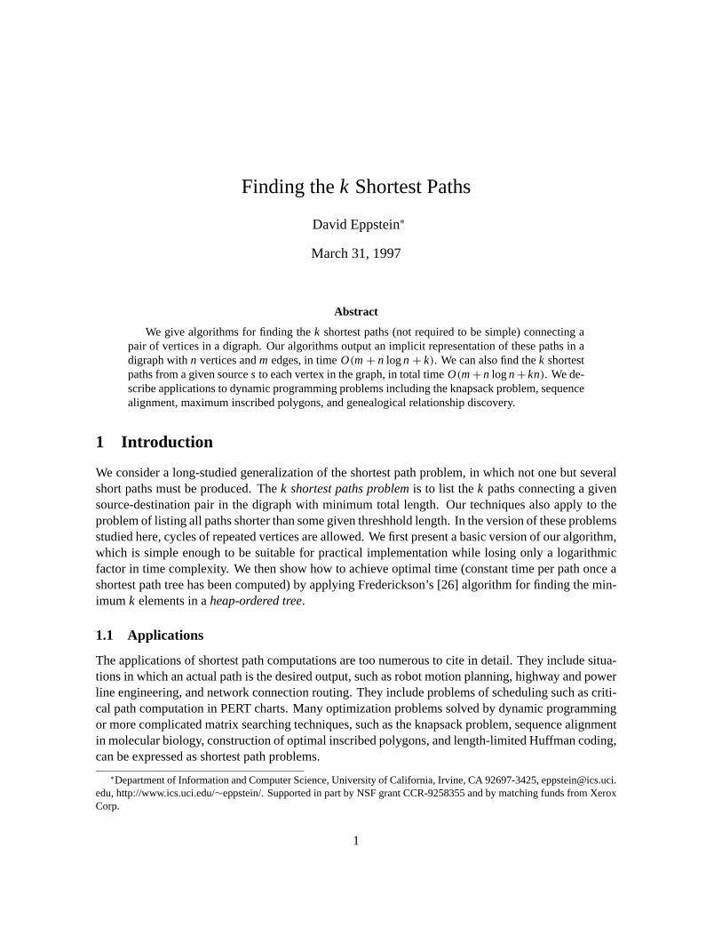
Figure 7. Some short relations in a complicated genealogical database.

5.4 Genealogical Relations

If one has a database of family relations, one may often wish to determine how some two individu-als in the database are related to each other. Formalizing this, one may draw a DAG in which nodesrepresent people, and an arc connects a parent to each of his or her children. Then each different typeof relationship (such as that of being a half-brother, great-aunt, or third cousin twice removed) can berepresented as a pair of disjoint paths from a common ancestor (or couple forming a pair of commonancestors) to the two related individuals, with the specific type of relationship being a function of thenumbers of edges in each path, and of whether the paths begin at a couple or at a single common an-cestor. In most families, the DAG one forms in this way has a tree-like structure, and relationshipsare easy to find. However in more complicated families with large amounts of intermarriage, one canbe quickly overwhelmed with many different relationships. For instance, in the British royal family,Queen Elizabeth and her husband Prince Philip are related in many ways, the closest few being sec-ond cousins once removed through King Christian IX of Denmark and his wife Louise, third cousins

20

through Queen Victoria of England and her husband Albert, and fourth cousins through Duke LudwigFriedrich Alexander of Wurttemberg and his wife Henriette (Figure 7). The single shortest relationshipcan be found as a shortest path in a graph formed by combining the DAG with its reversal, but longerpaths in this graph do not necessarily correspond to disjoint pairs of paths. A program I and my wifeDiana wrote, Gene (http://www.ics.uci.edu/∼eppstein/gene/), is capable of finding small numbers ofrelationships quickly using a backtracking search with heuristic pruning, but Gene starts to slow downwhen asked to produce larger numbers of relationships.

We now describe a technique for applying our k-shortest-path algorithm to this problem, based on amethod of Perl and Shiloach [48] for finding shortest pairs of disjoint paths in DAGs. Given a DAG D,we construct a larger DAG D1 as follows. We first find some topological ordering of D, and let f (x)represent the position of vertex x in this ordering. We then construct one vertex of D1 for each orderedpair of vertices (x, y) (not necessarily distinct) in D. We also add one additional vertex s in D1. Weconnect (x, y) to (x, z) in D1 if (y, z) is an arc of D and f (z) > max( f (x), f (y)). Symmetrically,we connect (x, y) to (z, y) if (x, z) is an arc of D and f (z) > max( f (x), f (y)). We connect s to allvertices in D1 of the form (v, v).

Lemma 13. Let vertices u and v be given. Then the pairs of disjoint paths in D from a common an-cestor a to u and v are in one-for-one correspondence with the paths in D1 from s through (a,a) to(u, v).

As a consequence, we can find shortest relationships between two vertices u and v by finding short-est paths in D1 from s to (u, v).

Theorem 8. Given a DAG with n nodes and medges, we can construct in O(mn) time a data structuresuch that, given any two nodes u and v in a DAG, we can list (an implicit representation of) the kshortest pairs of vertex-disjoint paths from a common ancestor to u and v, in time O(k). The samebound holds for listing all pairs with length less than a given bound (where k is the number of suchpaths). Alternately, the pairs of paths can be output in order by total length, in time O(log i ) to list thei th pair. As before, our representation allows constant-time computation of some simple functions ofeach path, and allows each path to be explicitly generated in time proportional to its length.

For a proof of Lemma 13 and more details of this application, see [19].

6 Conclusions

We have described algorithms for the k shortest paths problem, improving by an order of magnitudepreviously known bounds. The asymptotic performance of the algorithm makes it an especially promis-ing choice in situations when large numbers of paths are to be generated, and we there already exist atleast two implementations: one by Shibuya, Imai, et al. [52–55] and one by Martins (http://www.mat.uc.pt/∼eqvm/eqvm.html).

We list the following as open problems.

21

• The linear time construction when the shortest path tree is known is rather complicated. Is therea simpler method for achieving the same result? How quickly can we maintain heaps HT (v) ifnew leaves are added to the tree? (Lemma 4 solves this in O(log n) time per vertex but it seemsthat at least O(log log n) should be possible.)

• As described above, we can find the k best inscribed r -gons in an n-gon, in time O(rn3 + k).However the best single-optimum solution has the much faster time bound O(n log n+n

√r log n)

[1]. Our algorithms for the k best r -gons are efficient (in the sense that we use constant time perr -gon) only when k = Ä(rn3). The same phenomenon of overly large preprocessing times alsooccurs in our application to genealogical relationship finding: the shortest relationship can befound in linear time but our k-shortest-relationship method takes time O(mn+ k). Can we im-prove these bounds?

• Are there properties of paths not described by monoids which we can nevertheless compute ef-ficiently from our representation? In particular how quickly can we test whether each path gen-erated is simple?

Acknowledgements

This work was supported in part by NSF grant CCR-9258355. I thank Greg Frederickson, Sandy Iraniand George Lueker for helpful comments on drafts of this paper.

References

[1] A. Aggarwal, B. Schieber, and T. Tokuyama. Finding a minimum weight K -link path in graphswith Monge property and applications. Proc. 9th Symp. Computational Geometry, pp. 189–197.Assoc. for Computing Machinery, 1993.

[2] R. K. Ahuja, K. Mehlhorn, J. B. Orlin, and R. E. Tarjan. Faster algorithms for the shortest pathproblem. J. Assoc. Comput. Mach. 37:213–223. Assoc. for Computing Machinery, 1990.

[3] J. A. Azevedo, M. E. O. Santos Costa, J. J. E. R. Silvestre Madeira, and E. Q. V. Martins. Analgorithm for the ranking of shortest paths. Eur. J. Operational Research 69:97–106, 1993.

[4] A. Bako. All paths in an activity network. Mathematische Operationsforschung und Statistik7:851–858, 1976.

[5] A. Bako and P. Kas. Determining the k-th shortest path by matrix method. Szigma 10:61–66,1977. In Hungarian.

[6] R. E. Bellman. On a routing problem. Quart. Appl. Math. 16:87–90, 1958.

[7] A. W. Brander and M. C. Sinclair. A comparative study of k-shortest path algorithms. Proc. 11thUK Performance Engineering Worksh. for Computer and Telecommunications Systems, Septem-ber 1995.

22

[8] T. H. Byers and M. S. Waterman. Determining all optimal and near-optimal solutions when solv-ing shortest path problems by dynamic programming. Operations Research 32:1381–1384, 1984.

[9] P. Carraresi and C. Sodini. A binary enumeration tree to find K shortest paths. Proc. 7thSymp. Operations Research, pp. 177–188. Athenaum/Hain/Hanstein, Methods of Operations Re-search 45, 1983.

[10] G.-H. Chen and Y.-C. Hung. Algorithms for the constrained quickest path problem and the enu-meration of quickest paths. Computers and Operations Research 21:113–118, 1994.

[11] Y. L. Chen. An algorithm for finding the k quickest paths in a network. Computers and OperationsResearch 20:59–65, 1993.

[12] Y. L. Chen. Finding the k quickest simple paths in a network. Information Processing Letters50:89–92, 1994.

[13] E. I. Chong, S. R. Maddila, and S. T. Morley. On finding single-source single-destination k short-est paths. Proc. 7th Int. Conf. Computing and Information, July 1995. http://phoenix.trentu.ca/jci/papers/icci95/A206/P001.html.

[14] A. Consiglio and A. Pecorella. Using simulated annealing to solve the K -shortest path problem.Proc. Conf. Italian Assoc. Operations Research, September 1995.

[15] Y. Dai, H. Imai, K. Iwano, and N. Katoh. How to treat delete requests in semi-online problems.Proc. 4th Int. Symp. Algorithms and Computation, pp. 48–57. Springer Verlag, Lecture Notes inComputer Science 762, 1993.

[16] M. T. Dickerson and D. Eppstein. Algorithms for proximity problems in higher dimensions. Com-putational Geometry Theory and Applications 5:277–291, 1996.

[17] S. E. Dreyfus. An appraisal of some shortest path algorithms. Operations Research 17:395–412,1969.

[18] El-Amin and Al-Ghamdi. An expert system for transmission line route selection. Int. PowerEngineering Conf, vol. 2, pp. 697–702. Nanyang Technol. Univ, Singapore, 1993.

[19] D. Eppstein. Finding common ancestors and disjoint paths in DAGs. Tech. Rep. 95-52, Univ. ofCalifornia, Irvine, Dept. Information and Computer Science, 1995.

[20] D. Eppstein. Ten algorithms for Egyptian fractions. Mathematica in Education and Research4(2):5–15, 1995. http://www.ics.uci.edu/∼eppstein/numth/egypt/.

[21] D. Eppstein, Z. Galil, and G. F. Italiano. Improved sparsification. Tech. Rep. 93-20, Univ. ofCalifornia, Irvine, Dept. Information and Computer Science, 1993. http://www.ics.uci.edu:80/TR/UCI:ICS-TR-93-20.

[22] D. Eppstein, Z. Galil, G. F. Italiano, and A. Nissenzweig. Sparsification – A technique for speed-ing up dynamic graph algorithms. Proc. 33rd Symp. Foundations of Computer Science, pp. 60–69. IEEE, 1992.

[23] L. R. Ford, Jr. and D. R. Fulkerson. Flows in Networks. Princeton Univ. Press, Princeton, NJ,1962.

23

[24] B. L. Fox. k-th shortest paths and applications to the probabilistic networks. ORSA/TIMS JointNational Mtg., vol. 23, p. B263, 1975.

[25] G. N. Frederickson. Ambivalent data structures for dynamic 2-edge-connectivity and k smallestspanning trees. Proc. 32nd Symp. Foundations of Computer Science, pp. 632–641. IEEE, 1991.

[26] G. N. Frederickson. An optimal algorithm for selection in a min-heap. Information and Compu-tation 104:197–214, 1993.

[27] M. L. Fredman and R. E. Tarjan. Fibonacci heaps and their uses in improved network optimiza-tion algorithms. J. Assoc. Comput. Mach. 34:596–615. Assoc. for Computing Machinery, 1987.

[28] M. L. Fredman and D. E. Willard. Trans-dichotomous algorithms for minimum spanning treesand shortest paths. Proc. 31st Symp. Foundations of Computer Science, pp. 719–725. IEEE, 1990.

[29] A. V. Goldberg. Scaling algorithms for the shortest paths problem. SIAM J. Computing24(3):494–504. Soc. Industrial and Applied Math., June 1995.

[30] V. Hatzivassiloglou and K. Knight. Unification-based glossing. Proc. 14th Int. Joint Conf.Artificial Intelligence, pp. 1382–1389. Morgan-Kaufmann, August 1995. http://www.isi.edu/natural-language/mt/ijcai95-glosser.ps.

[31] G. J. Horne. Finding the K least cost paths in an acyclic activity network. J. Operational ResearchSoc. 31:443–448, 1980.

[32] L.-M. Jin and S.-P. Chan. An electrical method for finding suboptimal routes. Int. Symp. Circuitsand Systems, vol. 2, pp. 935–938. IEEE, 1989.

[33] D. B. Johnson. A priority queue in which initialization and queue operations take O(log log D)time. Mathematical Systems Theory 15:295–309, 1982.

[34] N. Katoh, T. Ibaraki, and H. Mine. An O(Kn2) algorithm for K shortest simple paths in an undi-rected graph with nonnegative arc length. Trans. Inst. Electronics and Communication Engineersof Japan E61:971–972, 1978.

[35] N. Katoh, T. Ibaraki, and H. Mine. An efficient algorithm for K shortest simple paths. Networks12(4):411–427, 1982.

[36] P. N. Klein, S. Rao, M. H. Rauch, and S. Subramanian. Faster shortest-path algorithms for planargraphs. Proc. 26th Symp. Theory of Computing, pp. 27–37. Assoc. for Computing Machinery,1994.

[37] N. Kumar and R. K. Ghosh. Parallel algorithm for finding first K shortest paths. ComputerScience and Informatics 24(3):21–28, September 1994.

[38] A. G. Law and A. Rezazadeh. Computing the K -shortest paths, under nonnegative weighting.Proc. 22nd Manitoba Conf. Numerical Mathematics and Computing, pp. 277–280, Congr. Nu-mer. 92, 1993.

[39] E. L. Lawler. A procedure for computing the K best solutions to discrete optimization problemsand its application to the shortest path problem. Management Science 18:401–405, 1972.

24

[40] E. L. Lawler. Comment on computing the k shortest paths in a graph. Commun. Assoc. Comput.Mach. 20:603–604. Assoc. for Computing Machinery, 1977.

[41] E. Q. V. Martins. An algorithm for ranking paths that may contain cycles. Eur. J. OperationalResearch 18(1):123–130, 1984.

[42] S.-P. Miaou and S.-M. Chin. Computing k-shortest path for nuclear spent fuel highway trans-portation. Eur. J. Operational Research 53:64–80, 1991.

[43] E. Minieka. On computing sets of shortest paths in a graph. Commun. Assoc. Comput. Mach.17:351–353. Assoc. for Computing Machinery, 1974.

[44] E. Minieka. The K -th shortest path problem. ORSA/TIMS Joint National Mtg., vol. 23, p. B/116,1975.

[45] E. Minieka and D. R. Shier. A note on an algebra for the k best routes in a network. J. Inst.Mathematics and Its Applications 11:145–149, 1973.

[46] D. Naor and D. Brutlag. On near-optimal alignments of biological sequences. J. ComputationalBiology 1(4):349–366, 1994. http://cmgm.stanford.edu/∼brutlag/Publications/naor94.html.

[47] A. Perko. Implementation of algorithms for K shortest loopless paths. Networks 16:149–160,1986.

[48] Y. Perl and Y. Shiloach. Finding two disjoint paths between two pairs of vertices in a graph. J.Assoc. Comput. Mach. 25:1–9. Assoc. for Computing Machinery, 1978.

[49] J. B. Rosen, S.-Z. Sun, and G.-L. Xue. Algorithms for the quickest path problem and the enu-meration of quickest paths. Computers and Operations Research 18:579–584, 1991.

[50] E. Ruppert. Finding the k shortest paths in parallel. Proc. 14th Symp. Theoretical Aspects ofComputer Science, February 1997.

[51] T. Shibuya. Finding the k shortest paths by AI search techniques. Cooperative Research Reportsin Modeling and Algorithms 7(77):212–222. Inst. of Statical Mathematics, March 1995.

[52] T. Shibuya, T. Ikeda, H. Imai, S. Nishimura, H. Shimoura, and K. Tenmoku. Finding a realisticdetour by AI search techniques. Proc. 2nd Intelligent Transportation Systems, vol. 4, pp. 2037–2044, November 1995. http://naomi.is.s.u-tokyo.ac.jp/papers/navigation/suboptimal-routes/ITS%95/its.ps.gz.

[53] T. Shibuya and H. Imai. Enumerating suboptimal alignments of multiple biological sequencesefficiently. Proc. 2nd Pacific Symp. Biocomputing, pp. 409–420, January 1997. http://www-smi.stanford.edu/people/altman/psb97/shibuya.pdf.

[54] T. Shibuya and H. Imai. New flexible approaches for multiple sequence alignment. Proc. 1stInt. Conf. Computational Molecular Biology, pp. 267–276. Assoc. for Computing Machinery,January 1997. http://naomi.is.s.u-tokyo.ac.jp/papers/genome/recomb97.ps.gz.

[55] T. Shibuya, H. Imai, S. Nishimura, H. Shimoura, and K. Tenmoku. Detour queries in geo-graphical databases for navigation and related algorithm animations. Proc. Int. Symp. Cooper-ative Database Systems for Advanced Applications, vol. 2, pp. 333–340, December 1996. http://naomi.is.s.u-tokyo.ac.jp/papers/databases/codas96.ps.gz.

25

[56] D. R. Shier. Algorithms for finding the k shortest paths in a network. ORSA/TIMS Joint NationalMtg., p. 115, 1976.

[57] D. R. Shier. Iterative methods for determining the k shortest paths in a network. Networks6(3):205–229, 1976.

[58] D. R. Shier. On algorithms for finding the k shortest paths in a network. Networks 9(3):195–214,1979.

[59] C. C. Skicism and B. L. Golden. Solving k-shortest and constrained shortest path problems ef-ficiently. Network Optimization and Applications, pp. 249–282. Baltzer Science Publishers, An-nals of Operations Research 20, 1989.

[60] K. Sugimoto and N. Katoh. An algorithm for finding k shortest loopless paths in a directed net-work. Trans. Information Processing Soc. Japan 26:356–364, 1985. In Japanese.

[61] J. W. Suurballe. Disjoint paths in a network. Networks 4:125–145, 1974.

[62] R. E. Tarjan. Data Structures and Network Algorithms. CBMS-NSF Regional Conference Seriesin Applied Mathematics 44. Soc. Industrial and Applied Math., 1983.

[63] R. Thumer. A method for selecting the shortest path of a network. Zeitschrift fur OperationsResearch, Serie B (Praxis) 19:B149–153, 1975. In German.

[64] M. S. Waterman. Sequence alignments in the neighborhood of the optimum. Proc. Natl. Acad.Sci. USA 80:3123–3124, 1983.

[65] M. M. Weigand. A new algorithm for the solution of the k-th best route problem. Computing16:139–151, 1976.

[66] A. Wongseelashote. An algebra for determining all path-values in a network with application tok-shortest-paths problems. Networks 6:307–334, 1976.

[67] A. Wongseelashote. Semirings and path spaces. Discrete Mathematics 26:55–78, 1979.

[68] J. Y. Yen. Finding the K shortest loopless paths in a network. Management Science 17:712–716,1971.

[69] J. Y. Yen. Another algorithm for finding the K shortest-loopless network paths. Proc. 41st Mtg.Operations Research Society of America, vol. 20, p. B/185, 1972.

26