Finding Scientifically Interesting Places on Mars UsingRegion Discovery Algorithms

Wei Ding, Christoph F. Eick Tomasz F. StepinskiDan Jiang, Rachsuda Jiamthapthaksin Lunar and Planetary Institute

Jiyeon Choo, Rachana Parmar, Chun-Sheng Chen Houston, TX 77058, USA∗

Computer Science DepartmentUniversity of Houston, TX 77004, USA†

ABSTRACTMars is at the center of the solar system exploration efforts.Measurements collected by spacecrafts orbiting around theplanet has been processed and organized into raster or point-based datasets describing different aspects of Martian sur-face. Impressive knowledge about Mars was obtained bystudying individual datasets, but additional information canbe gained by data mining the fusion of disparate datasets.In this paper, we present a computational framework forregion discovery geared toward finding scientifically inter-esting sites on Mars using multiple datasets. A novel familyof density-based, representative-based, grid-based, and ag-glomerative clustering algorithms is proposed to find suchsites. These algorithms search for contiguous regions maxi-mizing a domain-expert-defined measure of interestingness.The proposed framework is used and evaluated in a casestudy in which we try to find sites in which extreme val-ues of rampart impact craters co-locate with subsurface ice.Studying geological context of such sites provides a domainexpert with an insight on a history of water on Mars. Thecase study features a mixture of raster and discrete datasets.Two approaches are explored to cope with this discrepancy.In the first approach, the raster is discretized and then re-gional co-location mining is applied. In the second approach,the point-based dataset is smoothed and transformed into adensity function and then collocation regions are found fromhotspots of the product of z-scores of the two densities. Thepaper also evaluates the potential of proposed frameworkfor addressing scientific enquires in planetary sciences andother branches of geoscience.

Categories and Subject DescriptorsI.5.3 [Clustering]: Algorithms, J.2 [Physical Sciences andEngineering]: Astronomy

General Terms∗tom@lpi.ursra.edu†{wding,ceick,djiang, rachsuda}@uh.edu

Figure 1: A Sample Example for Co-location Pat-terns.

Algorithms, Experimentation.

KeywordsSpatial Data Mining, Data Mining for Planetary Science,Co-location Mining, Clustering, Region Discovery

1. INTRODUCTIONThe goal of spatial data mining [10] is to automate the ex-traction of interesting and useful patterns that are not ex-plicitly represented in spatial datasets. Of particular inter-est to scientists are the techniques capable of finding sci-entifically meaningful regions in spatial data sets as theyhave many immediate applications in geoscience, medicalscience, social science etc. Applications of region discoveryinclude detection of hotspots with respect to a single classor a continuous variable, and co-location mining aimed atdetection of regions with elevated densities of 2 more con-tinuous or discrete variables. For example, figure 1 spatialdataset containing instances belonging to different classes,and identifies four regions in which the density of differentpairs of classes is elevated. Other applications of region dis-covery includes sequence and graph mining, association rulemining and scoping, and sampling.

The ultimate goal of region discovery research is to providesearch-engine-style capabilities to scientists in order to assistthem in utilizing region discovery techniques in a highly au-tomated fashion. This goal faces several challenges. First, a

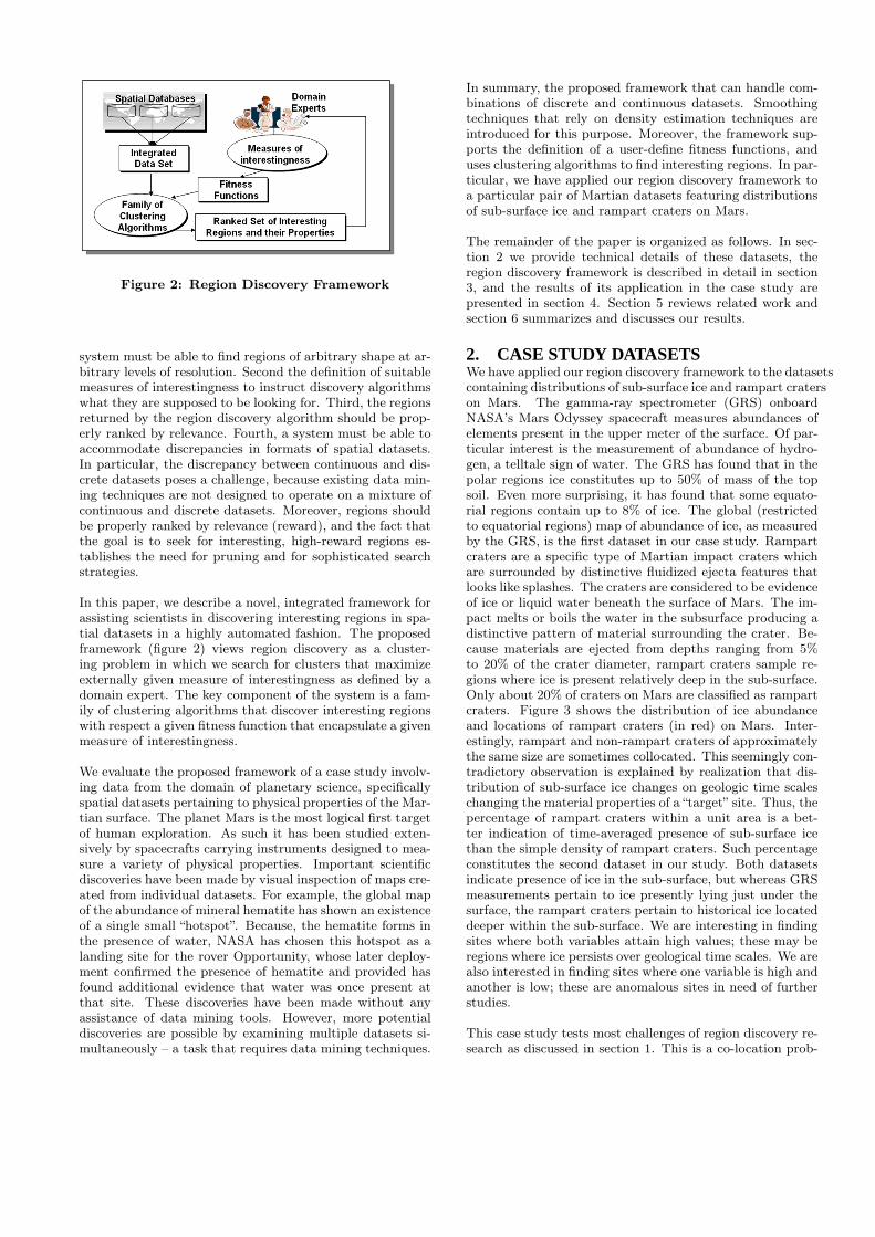
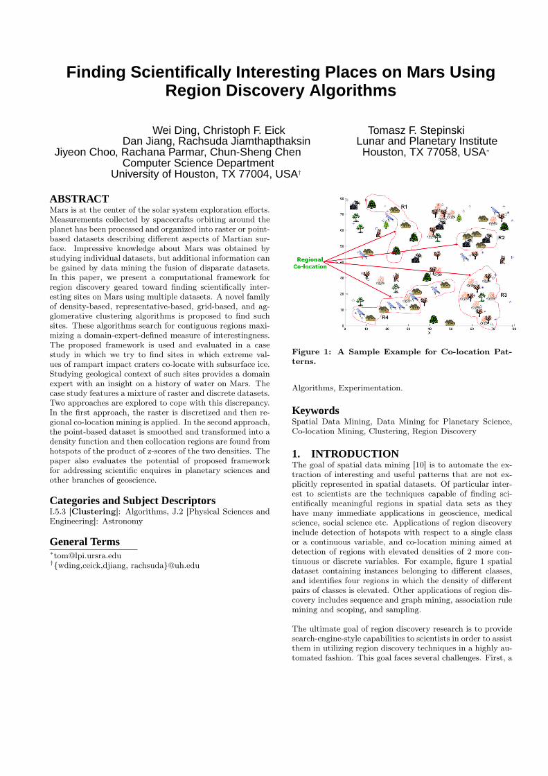
Figure 2: Region Discovery Framework

system must be able to find regions of arbitrary shape at ar-bitrary levels of resolution. Second the definition of suitablemeasures of interestingness to instruct discovery algorithmswhat they are supposed to be looking for. Third, the regionsreturned by the region discovery algorithm should be prop-erly ranked by relevance. Fourth, a system must be able toaccommodate discrepancies in formats of spatial datasets.In particular, the discrepancy between continuous and dis-crete datasets poses a challenge, because existing data min-ing techniques are not designed to operate on a mixture ofcontinuous and discrete datasets. Moreover, regions shouldbe properly ranked by relevance (reward), and the fact thatthe goal is to seek for interesting, high-reward regions es-tablishes the need for pruning and for sophisticated searchstrategies.

In this paper, we describe a novel, integrated framework forassisting scientists in discovering interesting regions in spa-tial datasets in a highly automated fashion. The proposedframework (figure 2) views region discovery as a cluster-ing problem in which we search for clusters that maximizeexternally given measure of interestingness as defined by adomain expert. The key component of the system is a fam-ily of clustering algorithms that discover interesting regionswith respect a given fitness function that encapsulate a givenmeasure of interestingness.

We evaluate the proposed framework of a case study involv-ing data from the domain of planetary science, specificallyspatial datasets pertaining to physical properties of the Mar-tian surface. The planet Mars is the most logical first targetof human exploration. As such it has been studied exten-sively by spacecrafts carrying instruments designed to mea-sure a variety of physical properties. Important scientificdiscoveries have been made by visual inspection of maps cre-ated from individual datasets. For example, the global mapof the abundance of mineral hematite has shown an existenceof a single small “hotspot”. Because, the hematite forms inthe presence of water, NASA has chosen this hotspot as alanding site for the rover Opportunity, whose later deploy-ment confirmed the presence of hematite and provided hasfound additional evidence that water was once present atthat site. These discoveries have been made without anyassistance of data mining tools. However, more potentialdiscoveries are possible by examining multiple datasets si-multaneously – a task that requires data mining techniques.

In summary, the proposed framework that can handle com-binations of discrete and continuous datasets. Smoothingtechniques that rely on density estimation techniques areintroduced for this purpose. Moreover, the framework sup-ports the definition of a user-define fitness functions, anduses clustering algorithms to find interesting regions. In par-ticular, we have applied our region discovery framework toa particular pair of Martian datasets featuring distributionsof sub-surface ice and rampart craters on Mars.

The remainder of the paper is organized as follows. In sec-tion 2 we provide technical details of these datasets, theregion discovery framework is described in detail in section3, and the results of its application in the case study arepresented in section 4. Section 5 reviews related work andsection 6 summarizes and discusses our results.

2. CASE STUDY DATASETSWe have applied our region discovery framework to the datasetscontaining distributions of sub-surface ice and rampart craterson Mars. The gamma-ray spectrometer (GRS) onboardNASA’s Mars Odyssey spacecraft measures abundances ofelements present in the upper meter of the surface. Of par-ticular interest is the measurement of abundance of hydro-gen, a telltale sign of water. The GRS has found that in thepolar regions ice constitutes up to 50% of mass of the topsoil. Even more surprising, it has found that some equato-rial regions contain up to 8% of ice. The global (restrictedto equatorial regions) map of abundance of ice, as measuredby the GRS, is the first dataset in our case study. Rampartcraters are a specific type of Martian impact craters whichare surrounded by distinctive fluidized ejecta features thatlooks like splashes. The craters are considered to be evidenceof ice or liquid water beneath the surface of Mars. The im-pact melts or boils the water in the subsurface producing adistinctive pattern of material surrounding the crater. Be-cause materials are ejected from depths ranging from 5%to 20% of the crater diameter, rampart craters sample re-gions where ice is present relatively deep in the sub-surface.Only about 20% of craters on Mars are classified as rampartcraters. Figure 3 shows the distribution of ice abundanceand locations of rampart craters (in red) on Mars. Inter-estingly, rampart and non-rampart craters of approximatelythe same size are sometimes collocated. This seemingly con-tradictory observation is explained by realization that dis-tribution of sub-surface ice changes on geologic time scaleschanging the material properties of a “target” site. Thus, thepercentage of rampart craters within a unit area is a bet-ter indication of time-averaged presence of sub-surface icethan the simple density of rampart craters. Such percentageconstitutes the second dataset in our study. Both datasetsindicate presence of ice in the sub-surface, but whereas GRSmeasurements pertain to ice presently lying just under thesurface, the rampart craters pertain to historical ice locateddeeper within the sub-surface. We are interesting in findingsites where both variables attain high values; these may beregions where ice persists over geological time scales. We arealso interested in finding sites where one variable is high andanother is low; these are anomalous sites in need of furtherstudies.

This case study tests most challenges of region discovery re-search as discussed in section 1. This is a co-location prob-

(a) (b)

Figure 3: (a) Distribution of Ice Abundance on Mars; (b) Locations of Rampart Craters on Mars(red: rampartcraters, green: non-rampart craters).

lem with mixed types of datasets where regions of interestmay occur on large and small scale.The standard way ofhandling data type discrepancy is to discretize the continu-ous dataset and then to apply co-location mining techniques,such as those proposed by Shekhar et. al. [11], to the dis-cretized data. In this paper, we also investigate the oppositeapproach that smooths the discrete dataset, using densityestimation techniques and z-score normalization, and thenperforms co-location mining on the product of two z-scoresin the continuous domain.

3. APPROACH EMPLOYEDWe first define the problem of regional discovery, and thenwe present our region discovery framework.

Let O = {o1, ..., on} be a set of spatial objects in the dataset.An object oi is defined as a vector of (x, y; <non-spatial at-tributes>), where x and y are spatial coordinates; for exam-ple, longitude and latitude. Spatial attributes are used tocompute spatial distances between clusters, while the non-spatial attributes are used by the fitness function for clus-tering evaluation. X = {c1, ..., ck} denotes a clustering solu-tion consisting of clusters c1 to ck where each cluster ci ⊆ O.Clusters occurring in the (x, y)-space identify interesting re-gions in the spatial space with respect to a given fitnessfunction. A region, in our approach, is defined as a set ofspatial objects belonging to a particular cluster ci. In thispaper we interchange the use of region and cluster.

The region discovery problem is defined as follows: Giventhe dataset O, a fitness function q(x) that evaluate clus-tering, we search for regions c1, ..., ck (a.k.a. clusters) suchthat:

1. The regions are disjoint: ci ∩ cj = Ø, i 6= j.

2. Each region are contiguous (each pair of objects be-longing to ci has to be Delaunay-connected with re-spect to ci).

3. X = {c1, ..., ck} maximizes q(X).

4. The generated regions are not required to be a totalpartition of the dataset O, that is, c1 ∪ ... ∪ ck ⊆ O.

5. c1, ..., ck are ranked based on the reward value. Re-gions that receive low rewards or no-rewards are fre-quently discarded.

3.1 Region Discovery FrameworkWe assume that the number of regions is not known in ad-vance, and therefore finding the best number of regions isone of the objectives of the clustering process. Therefore,our evaluation scheme has to be capable of comparing clus-tering schemes that contain different number of clusters.

Our region discovery algorithm employs a reward-based eval-uation scheme that evaluates the quality of the generated re-gions. Given regions X = {c1, ..., ck}, the fitness function isdefined as the sum of the rewards obtained from each regionri (i = 1..m) (Equation 1).

q(X) =∑c∈X

reward(c)

=∑c∈X

(ι(c)× |c|β), (1)

where ι is the interestingness function with respect to a mea-sure interestingness. |c|β(β > 1) in q(X) increases the valueof the fitness nonlinearly with respect to the region size |c|.Consequently, the evaluation scheme encourages merging re-gions with similar distribution if the overall rewards do notdecrease, because mathematically (aβ + bβ) < (a + b)β ifβ > 1.

Our framework views region discovery as a clustering prob-lem in which we search for clusters that maximize an exter-nally given measure of interestingness that captures whatdomain experts or interested in. The key feature is that theframework is designed to be able employ a family of clus-tering algorithms with respect to a set of measure of inter-estingness (function ι). It is a two-step procedure: We startwith a definition of measure of interestingness, and then wedetermine a threshold from which clusters are rewarded. Inthe following section, we will discuss how we employ clus-tering algorithms into our region discovery framework. wewill report the results of experiments in which the regiondiscovery algorithms, that were described in section 3.4, areused discovery such regions.

3.2 Measures of Interestingness and Their Cor-responding Fitness Functions

Two measures of interestingness have been designed to dealwith co-location mining for continuous and discrete datasets.Let Z = (< spatial attributes >; z) be the continuousdataset; in the remainder of this paper, we assume Z =(< x, y; z) where (x, y) represent longitude and latitudeand z is a continuous variable that is assumed to have amean of 0. We will discuss how to obtain attribute z insection 3.3. Let D = (< spatial attributes >; CL1, CL2)be the discrete dataset; in the rest of paper, we assumeD = (< x, y; CL1, CL2) where (x, y) represent longitudeand latitude and CL1, CL2 are class attributes for 3 classes,“low”, “normal”, and “high”.

Measure of interestingness for continuous co-locationmining.Given a continuous dataset Z, the interestingness functionιZ(c) with respect to cluster c is defined as

ιZ(c) =

{(|Σo.z

|c| | − zth)η if |Σo.z|c| | > zth

0 otherwise.(2)

where η > 1, zth > 0, o ∈cluster c and o.z is the value forattribute z of object o; |c| is the size of the cluster c; |Σo.z

|c| |is the absolute value for the mean value of z attribute incluster c; and zth is the reward threshold defined by user:only regions whose mean value for z is above zth receivepositive reward. In summary, this fitness function assignshigh rewards to regions that are hotspots and to regionsthat are cool spots with respect to variable z.

Measure of interestingness for binary co-location min-ing.Given a discrete dataset D, the goal is to assign high rewardsto regions in which the density of two classes CL1 and CL2

significantly deviates from the density of CL1 and CL2 inthe whole dataset. We define a multiplier λCL = p(CL,c)

prior(CL),

where P (CL, c) is the probability of objects in cluster c be-longing to class CL, and prior(CL) is the probability ofobjects in datasets D belonging to the CL. In general, mul-tiplier λCLi are computed for every cluster c, indicating howmuch the density of instances of class CL is elevated in clus-ter c compared to CL′s density in the whole space, andthe interestingness of a region with respect to two classesCL1 and CL2 is assessed proportional to the product of(|log2λc1 | − thc1) and (|log2λc2 | − thc2):

ιco−location(c) =if |log2λc1 | > thc1 and |log2λc2 | > thc2

(√

(|log2λc1 | − thc1)× (|log2λc2 | − thc2))η

otherwise,0

(3)

where th > 0, η > 1. For example, given a dataset with twoclasses, each class attribute contains “low”, “normal”, and“high”, 3 classes. The measure of interestingness ιco−location(c)is applied to 4 pairs of comparison: low/high, high/low,

low/low, and high/high. For the first pair of comparison,we compute the multiplier λCL for the “low” of the firstclass, and the “high” for the second class. For the other paircomparison, we compute the multiplier accordingly. Andthen we measure the interestingess of a cluster c using eachcorrespondent multiplier.

3.3 How to Address the Continuous DiscreteCo-location Problem

Our case study features a mixture of raster and discretedatasets. In particular, ice data are continuous, whereascrater data are discrete. The standard way of dealing withsuch a discrepancy is to discretize the continuous datasetand then to apply co-location mining techniques, such asthose proposed by Shekhar et. al. [11], to the discretizeddata. In this paper, we also investigate the opposite ap-proach that smoothes the discrete dataset, using z-scorenormalization, and then performs co-location mining on theproduct of two z-scores in the continuous domain. The re-mainder of this section discusses the two approaches in moredetail.

The first approach, for each crater o in the dataset we wrap afixed size window around o, and compute the number of ram-part craters, denoted number-ramp and the ratio of rampartcraters to all craters, denoted by ratio-ramp, in that window.Moreover, we look up the ice-density of all craters in thewindow, and take their mean-value and associate this mean-value with z using a variable called ice-density, denoted asρice. Next we take the so obtained datasets and apply z-score normalization to the number-ramp, ratio-ramp, andρice that replace a value v of attribute a by a new value:v−mean(a)variance(a)

, where mean(a) is the mean-value of attributea, and variance(a) is the variance of attribute a obtain-ing a dataset (x, y, z, zs-ratio-ramp, zs-number-ramp, zs-ice); finally we create two datasets Ice-Ratio-Ramp (x, y, z1)and Ice-Number-Ramp(x, y, z2) with z1 =zs-ratio-ramp×zs-ice and z1 =zs-number-ramp×zs-ice. Figure 6 gives depictsthe density function psi for σ = 1.5 for the Ice-Ratio-Rampdataset. It should be noted that hotspots (maxima witha high positive density values) correspond to regions witha high co-location of ice-density and crater-ratio and thatcool spots (minima with a high negative density values) cor-respond to regions for which high ice density is co-locatedwith low crater-ration or vice versa. In section 4, we will re-port the results of experiments in which the region discoveryalgorithms, that will be described in section 3.4, are used todiscover such regions.

The second approach, which is the typical approach of pastco-location research, discretizes the ice density into threeclasses: Ice-High, Ice-Normal, and Ice-Low, and looks forco-location patterns between those instances and instancesthat belong to the discretized classes Rampart-Ratio-High,Rampart-Ratio-Normal, and Rampart-Ratio-Low, basicallyfollowing the approach that was summarized in our intro-ductory discussions of figure 1.

3.4 Clustering AlgorithmsThe proposed region discovery framework provides a familyof representative-based, grid-based, density-based and ag-glomerative clustering algorithms. The goal of this section

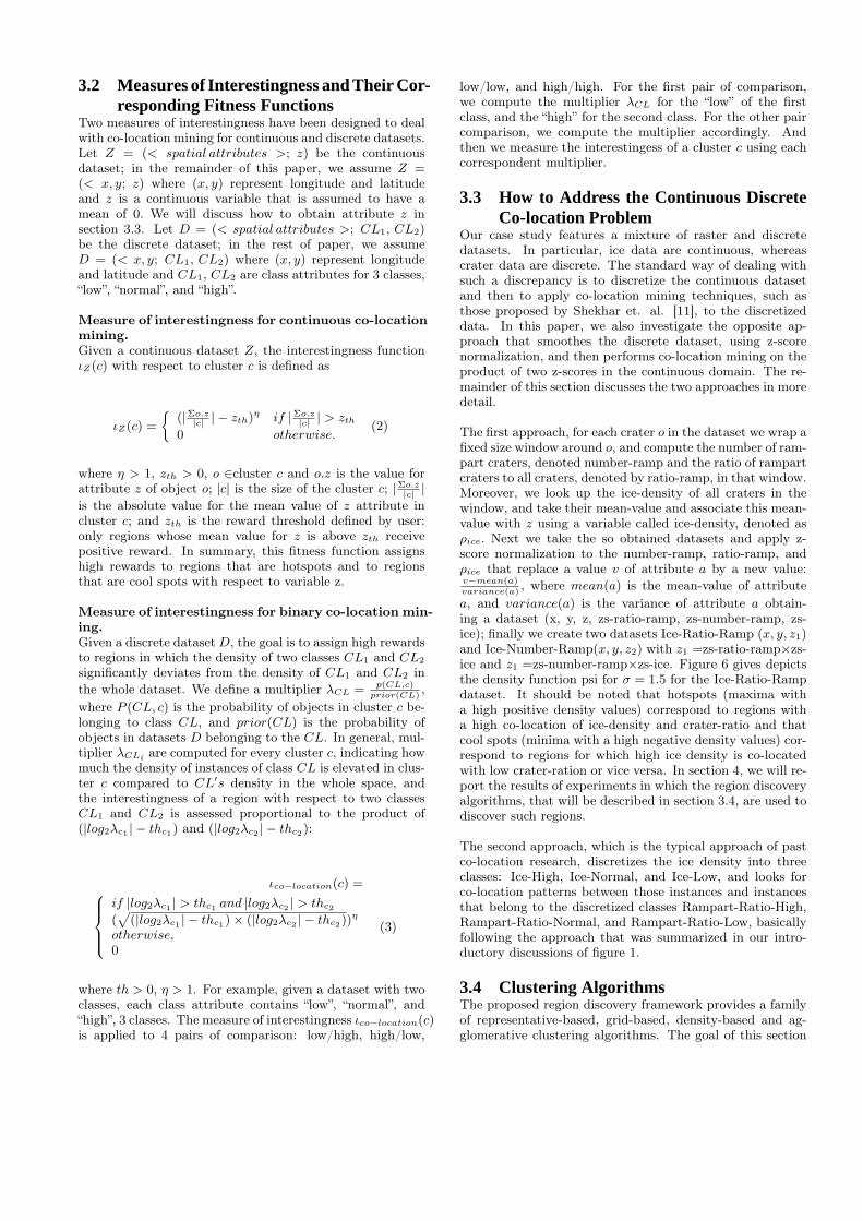
(a) (b)

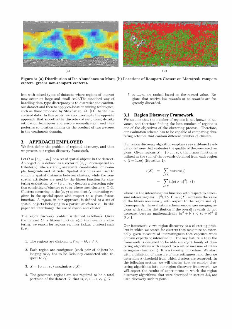
Figure 4: A Data set Contains 9 Complex Objects.(a) Input: 95 clusters generated by SPAM; (b) Out-put: 9 clusters identified by MOSAIC.

is to survey those algorithms that will later be used in a realworld case study that evaluates the region discovery frame-work.

Representative-based Clustering Algorithms.Representative-based clustering algorithms, sometime calledprototype based clustering algorithms in the literature, con-struct clusters by seeking for a set of representative; clus-ters are then created by assigning objects in the datasetto the closest representative. Popular representative-basedclustering algorithms are K-Medoids/PAM [6] and K-means[8]. Currently, we use a representative-based clustering al-gorithm, SPAM, for region discovery. SPAM (SupervisedPAM) is a variation of PAM. SPAM uses the fitness func-tion q(X) – and not the mean square error of the distanceof cluster objects to the cluster representative as PAM does– as its fitness function. SPAM starts its search with arandomly created set of representatives, and then greedilyreplace representatives with non-representatives as long asq(X) improves.

Agglomerative Algorithms.Due to the fact that representative-based algorithms con-struct clusters using nearest neighbor queries, the clustershapes that can be discovered are limited to convex polygons(Voronoi cells). However, in region discovery, frequently, in-teresting regions do not have convex shapes. MOSAIC [1]is an agglomerative clustering algorithm that approximatesarbitrary shape regions through the union of small convexpolygons, as depicted in Figure 4. MOSAIC uses a set of“small” clusters as its input (the name MOSAIC comes fromhere) – that have been obtained by running a representative-based region discovery algorithm, for example, SPAM witha large value for k – and greedily merges neighboring clus-ters as long as q(X) improves. Proximity graphs, namelyGabriel graphs1, are used to determine which clusters areneighboring. Algorithm 1 gives the pseudo code of the MO-SAIC algorithm.

Grid-based Algorithms.SCMRG (Supervised Clustering using Multi-Resolution Grids)[2, 13] is a hierarchical, grid-based method that utilizes a di-visive, top down search: The spatial space of the dataset is

1Gabriel graph is used to determine which clusters are neigh-boring. Two representative are said to be Gabriel neighborsif their diametric sphere does not contain any other repre-sentatives. For details, see [1], a master thesis done by oneof the co-authors.

Algorithm 1 Pseudo Code of MOSAIC.Input:

• A fitness function q(X).

Output:

• A set of optimal clusters X = {c1, ..., ck}.

1. Run a representative-based clustering algorithm, forexample, SCEC or SPAM, to create a large number ofclusters.

2. Obtain the representatives for clusters.

3. Construct a list of merge candidates using the repre-sentatives with a proximity graph.

4. Merge the pair of merge-candidates (ci, cj), that im-prove the fitness q(X) the most, go to Step 3; if nomore merge-candidates can improve the fitness, go toStep 5.

5. Return the best clustering X found.

partitioned into grid cells. Each grid cell at a higher level ispartitioned further into a number of smaller cells at the lowerlevel, and this process continues if the sum of the rewards ofthe lower level cells is greater than the rewards at the higherlevel cells. The regions returned by SCMRG usually havedifferent sizes, because they were obtained at different levelof resolution. Moreover, the algorithm captures clusteringinformation associated with spatial cells without recourseto the individual objects. In addition, a cell is only drilleddown if it is promising (if its fitness improves at a lower levelof resolution).

Density-Based Algorithms.In region discovery we are frequently confronted with theproblem to find regions with unexpected low or high valuesof a continuous variable z in a spatial dataset Z = (x, y; z)where (x, y) represent longitude and latitude and z is a con-tinuous variable that is assumed to have a mean of 0. Thedeviations of variable z from its mean can be upward de-viations, expressed by positive values of z, or downwarddeviations, expressed by negative values of z. SCDE (Su-pervised Clustering Using Density Estimation) is a density-based clustering algorithm that operates on density func-tions that have been constructed using Gaussian kernel den-sity estimation techniques for such datasets Z. The waySCDE constructs clusters is more or less identical with theway the popular, density-based clustering DENCLUE [4]computes clusters. However, it is important to stress thatthere are major differences between the density function Ψ,SCDE operates on, and the one DENCLUE employs. Inour approach, the density, Ψ(p) at point p is computed asfollows:

Ψ(p) =∑o∈Z

fGauss(p, o), (4)

The influence function, fGauss(p, o), uses the product of aGaussian kernel with the value of z of object o:

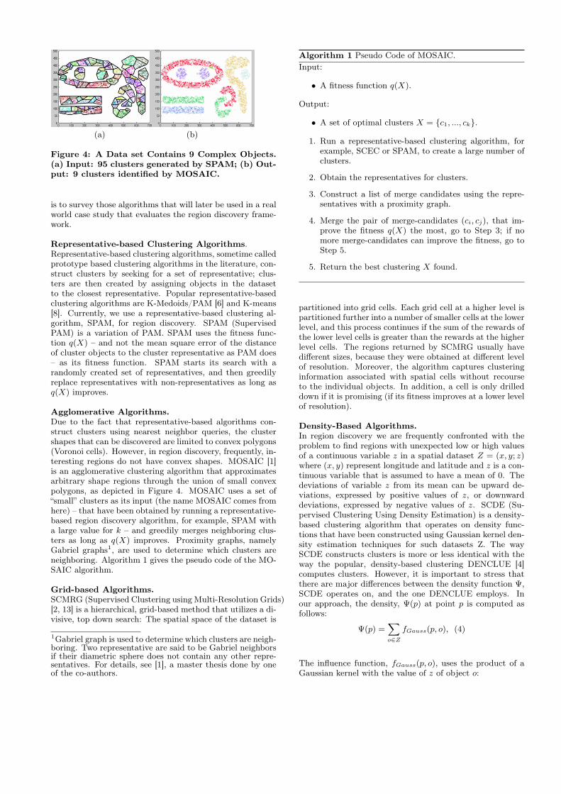
(a) (b)

Figure 5: Density Map for Co-location Patterns Be-tween Ratio of Rampart Craters and Ice Density.

fGauss(p, o) = o.z × e− d(p,o)2

2σ2 (5)

where d(p, o) is the distance between o and p. The parameterσ determines how quickly the influence of point o ∈ Z onthe density in point p decreases, as the distance between pand o increases.

SCDE created clusters using a hill climbing algorithm thatcomputes density attractors that are local maxima and min-ima of Ψ, and forms clusters by associating objects in thedataset with density attractors, whereas DENCLUE onlyconsiders local maxima. Moreover, we claim that if ∀o ∈ O :o.z = 1 holds, SCDE degenerate to DENCLUE. Finally, ifz is a class variable that takes values +1 and −1, SCDEbecomes a supervised clustering algorithm that computesregions that have a high percentage of examples of class +1,and regions that have high percentage of examples of class−1; in this case, points p = (x, y) for which Ψ(p) = 0 formdecision boundaries between the two classes in which thereis a complete balance between instances of the two classes.

Figure 5 gives the density function for the dataset Ice −Ratio− Ramp(x, y, z1) discussed in section 3.3. In the dis-play red hills depict locations in which high/low density oframpart craters co-locate with high/low density of ice, andblue upside down hills indicate locations in which high/lowdensity of rampart craters co-locates with low/high densitiesof ice.

In summary, the employed density estimation approach useskernels that can take negative values. To the best of ourknowledge, there are no publications in the data miningand machine learning literature that employs this approach.However, in a well-known book on density estimation [12]Silverman observes “there are some arguments in favor of us-ing kernels that take negative as well as positive values...thesearguments have first put forward by Parzen in 1962 andBartlett in 1963 ”.

4. EXPERIMENTAL EVALUATION4.1 Experiments ConductedWe use and evaluate our region discovery framework to findco-location patterns between rampart craters and ice abun-dance, using an ice raster density and a crater point datasets.We used four different clustering algorithms in the experi-ment: density-based (SCDE), representative-based (SPAM),grid-based (SCMRG), and agglomerative (MOSAIC) clus-tering algorithms. The inputs for MOSAIC is generated byrunning SPAM with k set to 400. As described in section

3.3, we have investigated two different co-location miningapproaches: (1) smooth the discrete dataset, using densityestimation techniques and z-score normalization, and thenperform co-location mining on the product of two z-scoresin the continuous domain; (2) discretize both datasets intoLow, Normal, and High, and then seek for regions where thedensity of 4 pair of classes is elevated (low/low, high/low,low/high, high/high). In the remainder of this section, wewill present experimental results for both approaches.

We have implemented our clustering algorithm using JavaJDK 1.5. All the clustering algorithms are part of ourCougar^2 Java library [9], which is an open source projectsupported by the UH-DMML Research group at the Univer-sity of Houston. All the experiments are conducted using 56dual processor nodes with 900 MHz processors, 2 nodes with1.3 GHz processors, and 2 nodes with 1.5 GHz Itanium2 pro-cessors.

4.2 Data Set PreprocessingThe ice raster density dataset is a 72× 36 matrix. Ice den-sities, ρice, are described in the scale of a cell size of 5 × 5degree2, where 1 degree corresponds to 59274.69752 meters.The crater dataset is a point-based dataset that contains35,927 craters. The location of each crater on Mars is de-scribed as a spatial point (x, y), using the longitude andlatitude.

For every crater (x, y), we determine the ice density at (x, y)by mapping the point (x, y) to the ice raster data set. Asdiscussed in section 3.3, we use 7 fixed window sizes togenerate 7 datasets for Ice-Ratio-Ramp (x, y, z1) and Ice-Number_Ramp (x, y, z2) respectively. Due to the fact thatice density is in the scale of 5×5 degree2, we chose 3 windowsizes above and below it with 2 by 2, 3 by 3, 4 by 4, 5 by 5,6 by 6, 7 by 7 and 8 by 8 degree2.

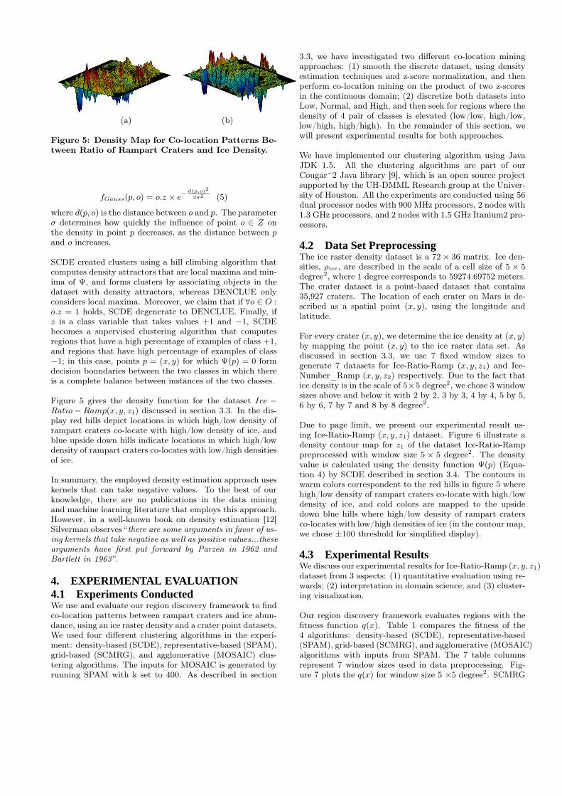
Due to page limit, we present our experimental result us-ing Ice-Ratio-Ramp (x, y, z1) dataset. Figure 6 illustrate adensity contour map for z1 of the dataset Ice-Ratio-Ramppreprocessed with window size 5 × 5 degree2. The densityvalue is calculated using the density function Ψ(p) (Equa-tion 4) by SCDE described in section 3.4. The contours inwarm colors correspondent to the red hills in figure 5 wherehigh/low density of rampart craters co-locate with high/lowdensity of ice, and cold colors are mapped to the upsidedown blue hills where high/low density of rampart cratersco-locates with low/high densities of ice (in the contour map,we chose ±100 threshold for simplified display).

4.3 Experimental ResultsWe discuss our experimental results for Ice-Ratio-Ramp (x, y, z1)dataset from 3 aspects: (1) quantitative evaluation using re-wards; (2) interpretation in domain science; and (3) cluster-ing visualization.

Our region discovery framework evaluates regions with thefitness function q(x). Table 1 compares the fitness of the4 algorithms: density-based (SCDE), representative-based(SPAM), grid-based (SCMRG), and agglomerative (MOSAIC)algorithms with inputs from SPAM. The 7 table columnsrepresent 7 window sizes used in data preprocessing. Fig-ure 7 plots the q(x) for window size 5 ×5 degree2. SCMRG

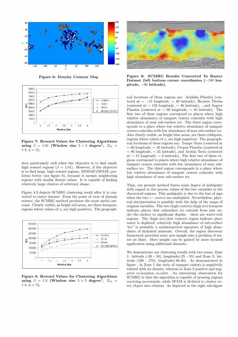
Figure 6: Density Contour Map

Figure 7: Reward Values for Clustering Algorithmsusing β = 1.01 (Window size 5 × 5 degree2, Zth =1.4, η = 1).

does particularly well when the objective is to find small,high reward regions (β = 1.01). However, if the objectiveis to find large, high reward regions, MOSAIC(SPAM) per-forms better (see figure 8), because it merges neighboringregions with similar fitness values. It is capable of findingrelatively large clusters of arbitrary shape.

Figure 4.3 depicts SCMRG clustering result after it is con-verted to raster dataset. From the point of view of domainscience, the SCMRG method produces the most useful out-come. Clearly visible, as bright red areas, are three hotspots,regions where values of z1 are high positives. The geograph-

Figure 8: Reward Values for Clustering Algorithmsusing β = 1.2 (Window size 5 × 5 degree2, Zth =1.4, η = 1).

Figure 9: SCMRG Results Converted To RasterDataset (left bottom corner coordinates (−180 lon-gitude, −90 latitude).

ical locations of these regions are: Acidalia Planitia (cen-tered at ∼ −15 longitude, ∼ 40 latitude), Hecates Tholus(centered at ∼ 150 longitude, ∼ 40 latitude), , and ArgyrePlanitia (centered at ∼ 60 longitude, ∼ 45 latitude). Thefirst two of these regions correspond to places where highrelative abundance of rampart craters coincides with highabundance of near sub-surface ice. The third region corre-sponds to a place where low relative abundance of rampartcraters coincides with low abundance of near sub-surface ice.Also clearly visible, as bright blue areas, are three coldspots,regions where values of z1 are high negatives. The geograph-ical locations of these regions are: Tempe Terra (centered at∼ 60 longitude, ∼ 45 latitude), Utopia Planitia (centered at∼ 90 longitude, ∼ 45 latitude), and Arabia Terra (centeredat ∼ 15 longitude, ∼ 0 latitude). The first two of these re-gions correspond to places where high relative abundance oframpart craters coincides with low abundance of near sub-surface ice. The third region corresponds to a place wherelow relative abundance of rampart craters coincides withhigh abundance of near sub-surface ice.

Thus, our present method leaves some degree of ambiguitywith regard to the precise values of the two variables in thediscovered regions. This ambiguity is due to the loss of signwhen the two z− scores are multiplied. Nevertheless, phys-ical interpretation is possible with the help of the maps oforiginal variables. The two (high craters)-(high ice) hotspotsindicate places that subsurface ice extends from just un-der the surface to significant depths – these are water-richregions. The (high ice)-(low craters) region indicate placewater is depleted; relatively high abundance of sub-surface“ice” is probably a misinterpreted signature of high abun-dance of hydrated minerals. Overall, the region discoveryframework provided some new insight into a problem of wa-ter on Mars. More insight can be gained by more focusedapplication using additional datasets.

We demonstrate our clustering results with two zones, Zone1: latitude (-30 - 58), longitude(-25 - 55) and Zone 2: lat-itude (100 - 170), longitude(-40-40). As demonstrated infigure , in Zone 1 the ratio of rampart craters is negativelyrelated with ice density, whereas in Zone 2 positive and neg-ative co-location co-exist. An interesting observation forSCMRG is that the algorithm is capable of pruning regionsreceiving no-rewards, while SPAM is ill-fated to cluster ev-ery object into clusters. As depicted in the right sub-figure

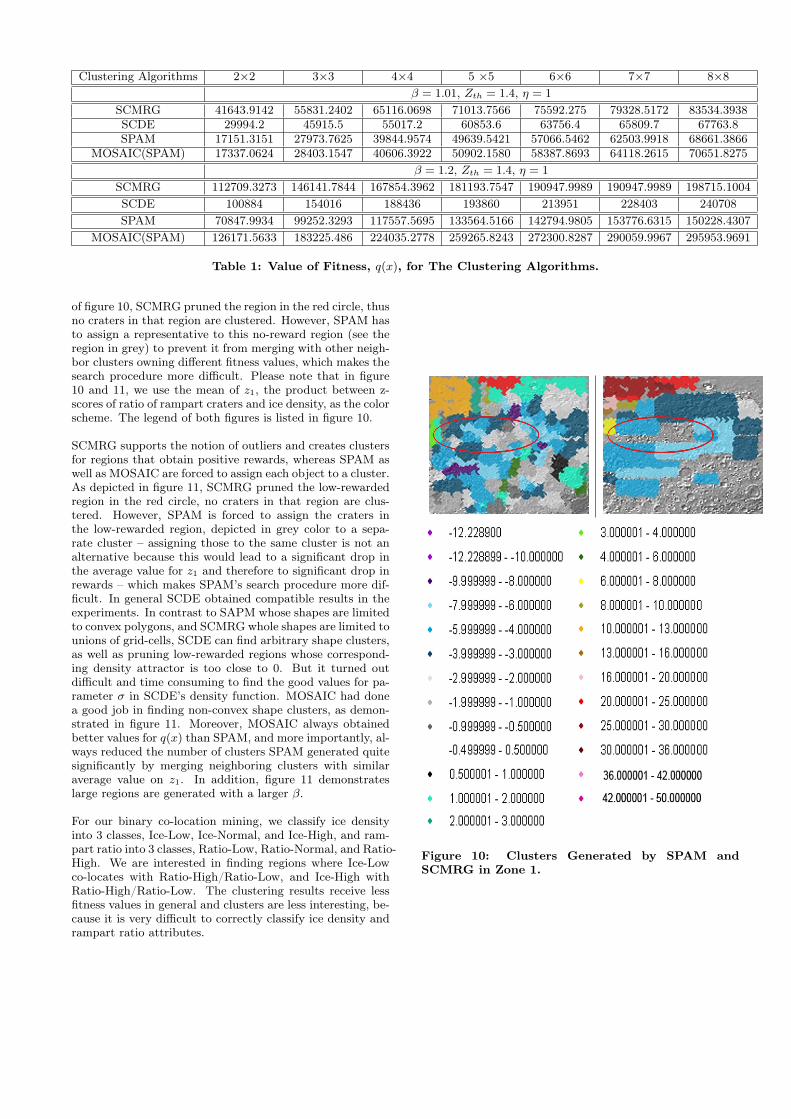
Clustering Algorithms 2×2 3×3 4×4 5 ×5 6×6 7×7 8×8β = 1.01, Zth = 1.4, η = 1

SCMRG 41643.9142 55831.2402 65116.0698 71013.7566 75592.275 79328.5172 83534.3938SCDE 29994.2 45915.5 55017.2 60853.6 63756.4 65809.7 67763.8SPAM 17151.3151 27973.7625 39844.9574 49639.5421 57066.5462 62503.9918 68661.3866

MOSAIC(SPAM) 17337.0624 28403.1547 40606.3922 50902.1580 58387.8693 64118.2615 70651.8275β = 1.2, Zth = 1.4, η = 1

SCMRG 112709.3273 146141.7844 167854.3962 181193.7547 190947.9989 190947.9989 198715.1004SCDE 100884 154016 188436 193860 213951 228403 240708SPAM 70847.9934 99252.3293 117557.5695 133564.5166 142794.9805 153776.6315 150228.4307

MOSAIC(SPAM) 126171.5633 183225.486 224035.2778 259265.8243 272300.8287 290059.9967 295953.9691

Table 1: Value of Fitness, q(x), for The Clustering Algorithms.

of figure 10, SCMRG pruned the region in the red circle, thusno craters in that region are clustered. However, SPAM hasto assign a representative to this no-reward region (see theregion in grey) to prevent it from merging with other neigh-bor clusters owning different fitness values, which makes thesearch procedure more difficult. Please note that in figure10 and 11, we use the mean of z1, the product between z-scores of ratio of rampart craters and ice density, as the colorscheme. The legend of both figures is listed in figure 10.

SCMRG supports the notion of outliers and creates clustersfor regions that obtain positive rewards, whereas SPAM aswell as MOSAIC are forced to assign each object to a cluster.As depicted in figure 11, SCMRG pruned the low-rewardedregion in the red circle, no craters in that region are clus-tered. However, SPAM is forced to assign the craters inthe low-rewarded region, depicted in grey color to a sepa-rate cluster – assigning those to the same cluster is not analternative because this would lead to a significant drop inthe average value for z1 and therefore to significant drop inrewards – which makes SPAM’s search procedure more dif-ficult. In general SCDE obtained compatible results in theexperiments. In contrast to SAPM whose shapes are limitedto convex polygons, and SCMRG whole shapes are limited tounions of grid-cells, SCDE can find arbitrary shape clusters,as well as pruning low-rewarded regions whose correspond-ing density attractor is too close to 0. But it turned outdifficult and time consuming to find the good values for pa-rameter σ in SCDE’s density function. MOSAIC had donea good job in finding non-convex shape clusters, as demon-strated in figure 11. Moreover, MOSAIC always obtainedbetter values for q(x) than SPAM, and more importantly, al-ways reduced the number of clusters SPAM generated quitesignificantly by merging neighboring clusters with similaraverage value on z1. In addition, figure 11 demonstrateslarge regions are generated with a larger β.

For our binary co-location mining, we classify ice densityinto 3 classes, Ice-Low, Ice-Normal, and Ice-High, and ram-part ratio into 3 classes, Ratio-Low, Ratio-Normal, and Ratio-High. We are interested in finding regions where Ice-Lowco-locates with Ratio-High/Ratio-Low, and Ice-High withRatio-High/Ratio-Low. The clustering results receive lessfitness values in general and clusters are less interesting, be-cause it is very difficult to correctly classify ice density andrampart ratio attributes.

Figure 10: Clusters Generated by SPAM andSCMRG in Zone 1.

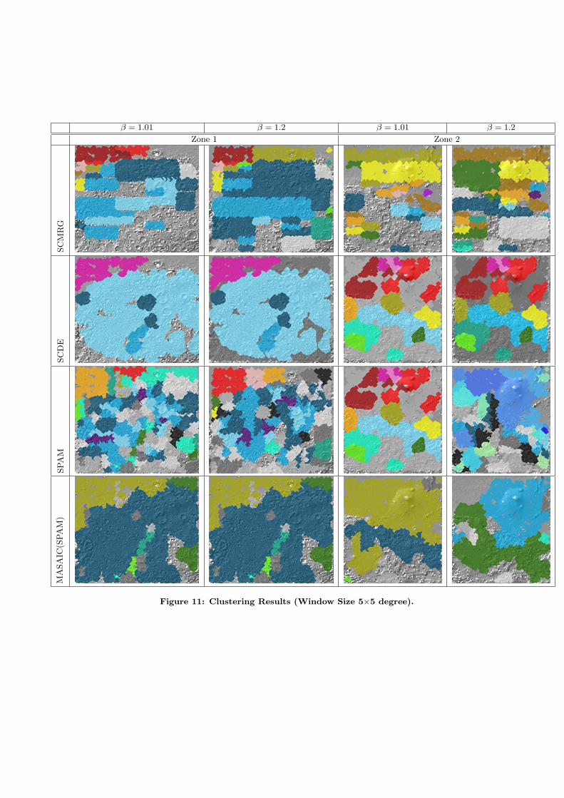
β = 1.01 β = 1.2 β = 1.01 β = 1.2

Zone 1 Zone 2

SCM

RG

SCD

ESP

AM

MA

SAIC

(SPA

M)

Figure 11: Clustering Results (Window Size 5×5 degree).

5. RELATED WORKPrevious work on rampart craters and sub-surface ice isabundant but not relevant to the topic of this paper. To ourbest knowledge, there have been no research work that em-ployed data mining techniques to the discovery of co-locationpatterns on Mars. The data mining areas most relevant toour work are: co-location mining, supervised clustering, andlocalized spatial statistics.

Shekhar et al. [11] discuss several interesting approachesto mine co-location pattern with respect to a given spatialevent. Yan Huang et al. [5] approach centers on co-locationmining of rare events and introduces a novel measure ofinterestingness for this purpose. Both approaches are re-stricted to discretized datasets, while our work aims to findco-location patterns in continuous datasets. Klösgen and M.May [7] propose a multi-relational framework for subgroupdiscovery within a spatial database system.

Localized spatial statistics [3] passes a moving window acrossthe spatial data, and examine dependence within the cho-sen region. Then they apply statistical analysis in the se-lected region. The major disadvantage is that the algorithmscannot analyze large datasets and their approach relies onextensive human interactions. Our framework aims to auto-mate the whole process and examine large spatial datasetsefficiently.

Supervised clustering [2] focuses on partitioning classifiedexamples, looking for hot spots that maximize cluster puritywhile keeping the number of clusters low. A framework forsupervised hotspot discovery has been introduced in [2]. Theframework introduced in this paper, on the other hand, isapplicable to both continuous and discrete datasets, allowsfor arbitrary fitness functions, and is applicable to a widevariety of region discovery problems, including co-locationmining, regional association rule mining and scoping, se-quence mining, variance analysis, and sampling.

6. CONCLUSIONRegion discovery in spatial datasets is a key technology forhigh impact scientific research, such as studying global cli-mate change and its effect to regional ecosystems; environ-mental risk assessment, modeling, and association analysisin planetary sciences. The paper introduces a novel, inte-grated framework that assists scientists in discovering in-teresting regions in spatial datasets in a highly automatedfashion. The framework treats region discovery as a cluster-ing problem in which we search for clusters that maximizean externally given measure of interestingness that captureswhat domain experts are interested in.

The framework was evaluated and tested in a case studythat center to find co-location patterns for a pair of Mar-tian datasets featuring distributions of sub-surface ice andrampart craters. A novel, regional co-location mining ap-proach was presented that searches for co-location patternsin the continuous domain, and measures the degree of co-location of two continuous variables as the product of their z-scores. Moreover, smoothing approaches for discrete datasetwere introduced that rely on density estimation techniques.In the approach was compared with the “traditional” co-location approach that discretizes continuous data sets and

performs co-location mining on discrete data sets. In thecase study, our z-score approach found a larger number ofinteresting regions than the traditional approach. Moreover,the z-score approach facilitates the automatic generation ofco-location maps that can be visually analyzed by domainexperts.

Finally, as a by-product, the paper introduces a novel den-sity estimation technique that relies on kernels that takenegative and positive values, and an agglomerative cluster-ing technique that merges neighboring regions greedily.

7. REFERENCES[1] Choo, J. Y. A hybrid clustering technique that

combines representative-based and agglomerativeclustering. Master’s thesis, December 2006. Advisor,Christoph F. Eick.

[2] Eick, C., Vaezian, B., Jiang, D., and Wang, J.Discovering of interesting regions in spatial data setsusing supervised cluster. In 10th European Conferenceon Principles and Practice of Knowledge Discovery inDatabases (PKDD’06) (2006).

[3] Getis, A., and Ord, J. K. Local spatial statistics:an overview. Spatial analysis: modeling in a GISenvironment (1996), 261–277.

[4] Hinneburg, A., and Keim, D. A. An efficientapproach to clustering in large multimedia databaseswith noise. In The 4th International Conference onKnowledge Discovery and Data Mining (KDD’98)(New York City, August 1998), pp. 58–65.

[5] Huang, Y., Pei, J., and Xiong, H. Miningco-location patterns with rare events from spatial datasets. Geoinformatica 10, 3 (2006), 239–260.

[6] Kaufman, L., and Rousseeuw, P. J. FindingGroups in Data: An Introduction to Cluster Analysis.John Wiley & Sons, 1990.

[7] Klösgen, W., and May, M. Spatial subgroupmining integrated in an object-relational spatialdatabase. In Principles of Data Mining and KnowledgeDiscovery Conference (PKDD) (2002), pp. 275–286.

[8] Lloyd, S. P. Least squares quantization in PCM.IEEE Trans. Information Theory 28 (1982), 128–137.(original version: Technical Report, Bell Labs), 1957.

[9] Mining, D., and Machine Learning Group, U.o. H. https://cougarsquared.dev.java.net/, 2007.

[10] Shekhar, S., and Chawla, S. Spatial Databases: ATour. Prentice Hall, 2003 (ISBN 013-017480-7), 2003.

[11] Shekhar, S., and Huang, Y. Discovering spatialco-location patterns: A summary of results. LectureNotes in Computer Science 2121 (2001).

[12] Silverman, B. Density Estimation for Statistics andData Analysis. Chapman & Hall, 1986.

[13] Wang, J. Region discovery using hierarchicalsupervised clustering. Master’s thesis, ComputerScience Department, Univeristy of Houston, 2006.