School of Innovation, Design and Engineering

Finding Optimum Batch Sizes for a High Mix, Low

Volume Surface Mount Technology Line

Master thesis work

30 credits, Advanced level

Product and process development Production and Logistics

Houtan Afshari

Report code: KPP231 Commissioned by: Westermo Teleindustri AB Tutor (company): Kari Parkkila, Christer Andersson Tutor (university): Antti Salonen Examiner: Sabah Audo

i

Abstract

Production of Printed Circuit Boards (PCBs) requires high-tech pick and place machines that

can produce significant number of boards in short time. However, increase in the variety of

boards causes interruptions in the production process. Frequent setups can lead to small lots

and low inventories. In contrast, bigger batch sizes save production time by having fewer

setups but they increase inventory value. Finding optimum batch sizes is a problem faced by

many manufacturers in a High mix, Low volume production environment.

In this thesis, the problem of finding optimum batch sizes is investigated using optimization

techniques in Operations Research. Furthermore, inspired by Single Minute Exchange of Die

theory, some improvements are suggested for the setup process. The conclusions from the

empirical part show that reducing setup times can help producing smaller batch sizes. It also

increases production capacity and system’s flexibility. Operations Research methods also

showed to be very effective tools that can lead to significant savings in terms of money and

capital.

Keywords: High mix-Low volume Production, Single Minute Exchange of Die (SMED),

Surface Mount Technology (SMT), Optimal Lot Sizing

ii

Acknowledgment

I would like to express my very great appreciation to Antti Salonen, my supervisor at MDH,

for his help and advice throughout this project. Special thanks to Sabah Audo, my professor in

Operations Research for his help during this thesis. I am particularly grateful to Christer

Andersson and Kari Parkkila, my supervisors in Westermo Teleindustri AB. Without their

valuable and constructive suggestions and their warm support, this report could not have been

realized.

At the end, I would also like to thank Heidi Panni-Pauninen for her friendship and kindness,

and the staff of Westermo for their patience and assistance in collection of my data.

iii

Table of Contents

List of Figures: ....................................................................................................................................... iv

List of Tables: .......................................................................................................................................... v

1. Introduction ..................................................................................................................................... 1

1.1 Background ............................................................................................................................. 1

1.2 Problem formulation ................................................................................................................ 2

1.3 Aim and research questions ..................................................................................................... 2

1.4 Project limitations .................................................................................................................... 2

2. Research method ............................................................................................................................. 4

2.1 Quantitative vs. Qualitative method ........................................................................................ 4

2.2 Case study................................................................................................................................ 5

2.3 Case company .......................................................................................................................... 6

2.4 Research method, data collection and analysis ....................................................................... 6

3. Theoretic framework ....................................................................................................................... 8

3.1 Description of an SMT line ..................................................................................................... 8

3.2 Economic Order Quantity...................................................................................................... 12

3.3 Discussion about setup cost ................................................................................................... 15

3.4 Single Minute Exchange of Die ............................................................................................ 16

3.4.1 Fundamentals of SMED ................................................................................................ 18

3.4.2 Discussion over SMED ................................................................................................. 19

3.5 Linear optimization, nonlinear optimization ......................................................................... 21

3.6 Exact methods, Heuristics ..................................................................................................... 21

3.6.1 Genetic Algorithm ......................................................................................................... 22

4. Results (Empirics) ......................................................................................................................... 24

4.1 Calculating EOQs .................................................................................................................. 24

4.2 Discussion over setup cost..................................................................................................... 28

4.3 Writing an optimization model .............................................................................................. 34

4.4 Solving the optimization model............................................................................................. 43

4.5 Setup improvement ................................................................................................................ 55

5. Analysis ......................................................................................................................................... 59

6. Conclusions and Recommendations .............................................................................................. 66

7. References ..................................................................................................................................... 68

8. Appendices .................................................................................................................................... 71

A. The GA code for MATLAB .................................................................................................. 71

B. Tables 12 to 14 ...................................................................................................................... 72

iv

List of Figures:

Figure 1: A printed circuit board (O-digital.com, 2014) ......................................................................... 8

Figure 2: A solder paste printing machine .............................................................................................. 9

Figure 3: A pick and place machine for small components .................................................................... 9

Figure 4: A pick and place machine for large components ................................................................... 10

Figure 5: A horizontal turret head rotating around z axis...................................................................... 10

Figure 6: A movable feeder carrier ....................................................................................................... 11

Figure 7: An inline reflow oven ............................................................................................................ 11

Figure 8: The cycle inventory (Krajewski, Ritzman and Malhotra, 2007) ............................................ 12

Figure 9: Annual holding cost (Krajewski, Ritzman and Malhotra, 2007) ........................................... 13

Figure 10: Annual setup cost (Krajewski, Ritzman and Malhotra, 2007) ............................................. 14

Figure 11: Annual total cost (Krajewski, Ritzman and Malhotra, 2007) .............................................. 14

Figure 12: Conceptual stages for setup improvement (Shingo, 1985) .................................................. 18

Figure 13: Limits and costs of changeover improvement strategies (Ferradás and Salonitis, 2013) .... 20

Figure 14: a) Elite child. b) Crossover child. c) Mutation child (Mathworks.se, 2014) ........................ 23

Figure 15: Annual total cost (Krajewski, Ritzman and Malhotra, 2007) .............................................. 33

Figure 16: Setup cost based on number of setups ................................................................................. 34

Figure 17: Annual demand for a board .................................................................................................. 35

Figure 18: Annual demand for a board .................................................................................................. 36

Figure 19: Annual demand for a board .................................................................................................. 36

Figure 20: Annual demand for a board .................................................................................................. 37

Figure 21: Simplified demand ............................................................................................................... 38

Figure 22: Changes in inventory level................................................................................................... 38

Figure 23: Customer demand for a board produced by customer order ................................................ 44

Figure 24: Demand for a prototype board ............................................................................................. 44

Figure 25: A panel with 25 PCBs (Pcbfabrication.com, 2014) ............................................................. 45

Figure 26: Lingo’s error message .......................................................................................................... 46

Figure 27: Lingo’s solver status ............................................................................................................ 47

Figure 28: Lingo’s interface .................................................................................................................. 47

Figure 29: MATLAB’s optimization toolbox ....................................................................................... 48

Figure 30: MATLAB’s optimization decision table.............................................................................. 48

Figure 31: Constraint function with only two variables ........................................................................ 49

Figure 32: Global Optimization Toolbox in MATLAB ........................................................................ 50

Figure 33: Table for Choosing a Solver ................................................................................................ 50

Figure 34: Optimization tool in MATLAB ........................................................................................... 51

Figure 35: Sorting feeders on the rack .................................................................................................. 57

Figure 36: Reduction in Inventory Value .............................................................................................. 59

Figure 37: Available time for production in a week .............................................................................. 63

Figure 38: Capacity reduction with setup time = 22 minutes ................................................................ 64

Figure 39: Capacity reduction with setup time = 15 minutes ................................................................ 64

Figure 40: Setup time reduction when capacity is fixed at two shifts ................................................... 65

v

List of Tables:

Table 1: Relationship between setup time and lot size (Shingo, 1985) ................................................. 16

Table 2: Relationship between setup time and lot size for a longer setup time (Shingo, 1985) ............ 17

Table 3: Relationship between setup time and lot size for a short setup time (Shingo, 1985) .............. 18

Table 4: The Economic Order Quantities calculated for boards ........................................................... 25

Table 5: The Economic Order Quantities calculated for boards ........................................................... 29

Table 6: Average inventory for a board ................................................................................................ 39

Table 7: Average inventory for a board ................................................................................................ 39

Table 8: Average inventory for a board ................................................................................................ 40

Table 9: Average inventory for a board ................................................................................................ 41

Table 10: Optimum batch sizes ............................................................................................................. 52

Table 11: Effect of setup time reduction on batch sizes ........................................................................ 60

Table 12: Reduction in work time requirements by steps of 3% when setup time is 22 minutes ......... 72

Table 13: Reduction in work time requirements by steps of 3% when setup time is 15 minutes ......... 75

Table 14: Reduction in setup time by steps of 1 minute when working time is fixed at 2 shifts .......... 79

vi

Abbreviations

DES Discrete Event Simulation

DIN Deutsches Institut für Normung

EOQ Economic Order Quantity

ERP Enterprise Resource Planning

GA Genetic Algorithm

HMC Hybrid Microcircuit

IDT Akademin för Innovation, Design och Teknik IED Inside Exchange of Die

IFS Industrial and Financial Systems

LP Linear Programming

MAPE Mean Absolute Percentage Error

MDH Mälardalens Högskola

MRP Materials Requirement Planning

NLP Nonlinear Programming

OED Outside Exchange of Die

OEE Overall Equipment Effectiveness

OR Operations Research

PCB Printed Circuit Board

R&D Research and Development

RS Recommended Standard

SAP Systems Applications Products

SMED Single-Minute Exchange of Die

SMT Surface Mount Technology

1

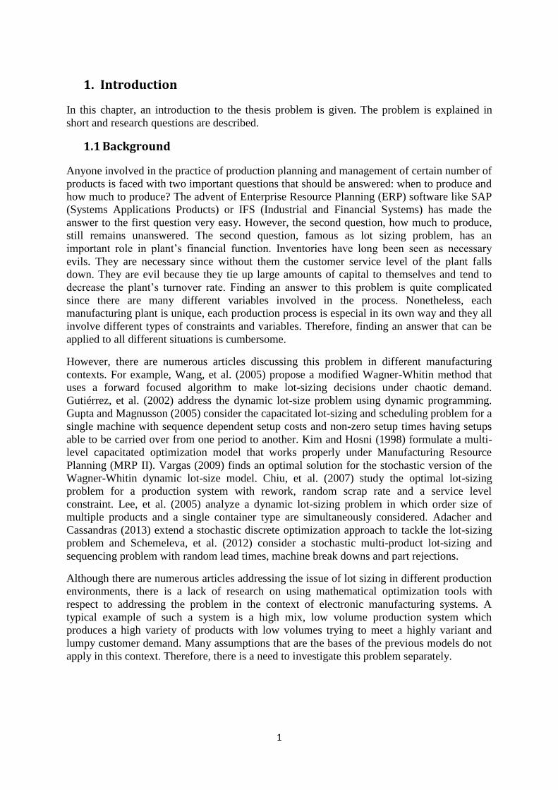
1. Introduction

In this chapter, an introduction to the thesis problem is given. The problem is explained in

short and research questions are described.

1.1 Background

Anyone involved in the practice of production planning and management of certain number of

products is faced with two important questions that should be answered: when to produce and

how much to produce? The advent of Enterprise Resource Planning (ERP) software like SAP

(Systems Applications Products) or IFS (Industrial and Financial Systems) has made the

answer to the first question very easy. However, the second question, how much to produce,

still remains unanswered. The second question, famous as lot sizing problem, has an

important role in plant’s financial function. Inventories have long been seen as necessary

evils. They are necessary since without them the customer service level of the plant falls

down. They are evil because they tie up large amounts of capital to themselves and tend to

decrease the plant’s turnover rate. Finding an answer to this problem is quite complicated

since there are many different variables involved in the process. Nonetheless, each

manufacturing plant is unique, each production process is especial in its own way and they all

involve different types of constraints and variables. Therefore, finding an answer that can be

applied to all different situations is cumbersome.

However, there are numerous articles discussing this problem in different manufacturing

contexts. For example, Wang, et al. (2005) propose a modified Wagner-Whitin method that

uses a forward focused algorithm to make lot-sizing decisions under chaotic demand. Gutiérrez, et al. (2002) address the dynamic lot-size problem using dynamic programming.

Gupta and Magnusson (2005) consider the capacitated lot-sizing and scheduling problem for a

single machine with sequence dependent setup costs and non-zero setup times having setups

able to be carried over from one period to another. Kim and Hosni (1998) formulate a multi-

level capacitated optimization model that works properly under Manufacturing Resource

Planning (MRP II). Vargas (2009) finds an optimal solution for the stochastic version of the

Wagner-Whitin dynamic lot-size model. Chiu, et al. (2007) study the optimal lot-sizing

problem for a production system with rework, random scrap rate and a service level

constraint. Lee, et al. (2005) analyze a dynamic lot-sizing problem in which order size of

multiple products and a single container type are simultaneously considered. Adacher and

Cassandras (2013) extend a stochastic discrete optimization approach to tackle the lot-sizing

problem and Schemeleva, et al. (2012) consider a stochastic multi-product lot-sizing and

sequencing problem with random lead times, machine break downs and part rejections.

Although there are numerous articles addressing the issue of lot sizing in different production

environments, there is a lack of research on using mathematical optimization tools with

respect to addressing the problem in the context of electronic manufacturing systems. A

typical example of such a system is a high mix, low volume production system which

produces a high variety of products with low volumes trying to meet a highly variant and

lumpy customer demand. Many assumptions that are the bases of the previous models do not

apply in this context. Therefore, there is a need to investigate this problem separately.

2

1.2 Problem formulation

Today there is a lack of knowledge and competence in companies regarding the use of

mathematical optimization for finding optimum batch sizes. The smaller batch sizes will

reduce the inventory and help the company toward production according to customer orders

which is one of the aims of Lean manufacturing. However, increased number of long setups

may decrease the available production time and expose the production line with the danger of

unmet customer demand. Bigger batch sizes will reduce the number of setups and increase the

available production time but they will also increase the inventory value. More products will

be in stock for a longer period of time and they are exposed to deterioration. There will also

be a need for a larger storage for keeping the items in stock. In addition, bigger batches are an

obstacle for producing a high mix of products. Due to longer production time of bigger

previous batches; each job should wait for a longer time until it can enter the line. The focus

of this thesis project is to answer this question: What are the optimum batch sizes for a High

mix, Low volume production line? In order to answer this question, two methods are used.

Economic Order Quantities (EOQ) is the first method that is tested. Followed by that, the use

of Operations Research (OR) techniques are investigated on lot sizing problem.

1.3 Aim and research questions

The aim of this project is to explore the potential of utilizing mathematical optimization tools

on a real case and to find a proper method to calculate the optimum batch sizes and to present

the results. There will also be an analysis of the capacity to investigate the effect that changes

in capacity can have on the system in terms of batch sizes, inventory value and ability to meet

customer demand. The capacity analysis part is performed due to the management request.

The research questions can be described as shown below:

What are the optimum batch sizes?

What is the relationship between setup times and batch sizes?

What is the relationship between setup times and inventory value?

What is the relationship between capacity with batch sizes and inventory value?

Is it possible to reduce the work time requirements and reduce the batch sizes at the

same time?

1.4 Project limitations

The main limitation for this project was time. More time could lead to more precise

evaluations of the current state and could give way to examine different methods to solve the

problem. Limited project time leads to early conclusions and less detailed work, with a variety

of methods untested.

During building the optimization model and preparing the input data, it was decided that some

of the boards should be excluded and not take part in the model. A series of these boards were

prototypes. Prototypes are occasionally produced and present boards that will be a part of

production flora in the future. However, they are not a part of companies products now and

they are not produced regularly. Therefore, it is not reasonable to involve them in the

optimization process since they can negatively influence the optimization result for other

boards.

There were two other groups of boards that went under the same decision. A set of boards

used to be produced regularly in the past but now their production has been discontinued. The

information related to these boards was combined with other boards and therefore it had to be

3

filtered out. Another group of boards are produced based on customer orders. The batch sizes

for these boards depend on the order size from customers. Therefore, it is not reasonable to

include them in the model.

The cycle times that are used in the model have been obtained from the companies data base.

The accuracy of these cycle times are not clear. However, it was not possible to measure the

cycle times personally due to the large number of different boards produced and due to the

shortage of time. Therefore, it was decided to trust these data and use them as an input for the

model.

In order to obtain the optimum batch sizes, the annual data for the year 2013 for each board

was used. Previous years were excluded and current year (2014) was not used either, since the

data for the remaining months of this year is not available yet. However, for the capacity

analysis part, the data for year 2014 was used (January to April). This was due to the

management request.

The part in the impirical section which gives suggestions regarding reducing setup times is

short despite the fact that the work on this section was thourough and numerous suggestions

were given. Reducing setup times influences batch sizes and is closely related to capacity

analysis, but since it is not the focus of this report, it was mentioned shortly. However, a

thourough description of the methods are given in the theoretical framework.

4

2. Research method

It is a matter of importance during any research process to let the research problem decide the

choice of approach and it is equally important to take its consequences into consideration.

Accordingly, research problem will determine the perspective and the perspective will decide

the choice of method (Johansson, 1995).

2.1 Quantitative vs. Qualitative method

Qualitative and quantitative research methods have long been two main research

methodologies among academia. Qualitative research is a method to explore and understand

the meaning individuals or groups give to a social or human problem. The research includes

the process of emerging questions and procedures, collection of data typically in the

participant’s settings, inductive analysis of data moving from particulars to general themes

and making interpretation of the data by the researcher (Creswell, 2009).

Quantitative research at the other hand, is a tool for testing objective theories through

examining the relationship among variables. These variables, in turn, can be measured and

turned into numbered data that can be analyzed using statistical procedures. The final report

of this research method should have a structure consisting introduction, literature and theory,

methods, results and discussion. Those involve in this type of research are interested in

deductive analysis and testing of theories, evaluating alternative explanations and being able

to generalize and replicate the findings (Creswell, 2009).

There are a set of differences between these two traditions. The most important difference

between them is the way in which each tradition treats data (Brannen, 1992). In quantitative

approach, the researcher tries to test a theory by specifying and narrowing down a hypotheses

and by collecting data to support or refute the hypotheses (Creswell, 2009). In theory, if not in

practice, the researcher defines and isolates variables and variable categories. The variables

then, are linked together to frame hypotheses often before the data is collected, and are then

tested upon the data (Brannen, 1992). The qualitative researcher at the other hand, begins with

defining very general concepts which will change in their definitions as the research

progresses. For the former, the variables are the tools and means of the analysis while for the

latter, they are the product or outcome of the research (Brannen, 1992). As an example, in

qualitative method, the researcher tries to establish the meaning of a phenomenon from the

views of participants. This requires to identify a culture-sharing group and to study how it

develops shared patterns of behavior over time (Creswell, 2009). The qualitative researcher is

said to look through a wide lens, looking for patterns of inter-relationship between a set of

concepts that are usually unspecified while the quantitative researcher looks through a narrow

lens at a set of specified variables (Brannen, 1992).

The second important difference between the two methods is the way they collect data. In the

qualitative tradition, the researcher must use himself as the instrument, attending to his own

cultural assumptions as well as to the data. In order to gain insights to the participants’ social

worlds the researcher is expected to be flexible and reflexive and yet manufacture some

distance (Brannen, 1992). Qualitative approach includes three main kinds of data collection

methods: in depth, open-ended interviews; direct observation; and written documents

(Johansson, 1995).

In quantitative tradition, the instrument is a finely tuned tool which allows for much less

flexibility, imaginative input and reflexivity, for example a questionnaire. By contrast, when

the research issue is less clear and questions to participants may result in complex answers,

5

qualitative methods like in-depth interviewing may be called for (Brannen, 1992). Compared

to qualitative method, the main quantitative research techniques include the use of

questionnaires, structured interviews, measurement, standardized tests, statistics and

experiments (Johansson, 1995).

Qualitative approach studies selected issues in depth and detail. This is due to the ability to

approach the fieldwork with openness and without being constrained by predetermined

categories of analysis. On the other hand, quantitative methods require the usage of

standardized methods so that the wide variety of perspectives and experiences of people can

be fitted into a small number of predetermined response categories. The most advanced

method in quantitative research is experiment where fieldwork is replaced by laboratory

(Johansson, 1995).

In quantitative approach, the researcher often tries to minimize the effects of intervening

factors on the research phenomenon. In qualitative approach, the researcher tries to find out

and describe what the intervening factors are and how they influence the research

phenomenon under study (Johansson, 1995).

In quantitative research, the researcher works with statistics and uses the average, the

frequency, the causality and the prediction as a base for the report. In qualitative research, the

researcher believes that if something has happened once, it can happen again even if you

cannot calculate where and when (Johansson, 1995).

2.2 Case study

As a research strategy, case study has been used in many different situations to contribute to

our understanding and knowledge about individual, group, organizational, social, political,

and related phenomena. Case study is even used in economics, where the structure of a given

industry or the economy of a given region or city is investigated by case study techniques. In

all of these cases, the need for a case study arises out of the desire to understand complex

phenomena. In brief, the case study allows the researcher to retain the holistic and meaningful

characteristics of real-life events (Yin, 2003).

Case study is defined as:

“An empirical inquiry that investigates a contemporary phenomenon within its real-

life context, especially when the boundaries between phenomenon and context are

not clearly evident. The case study inquiry copes with the technically distinctive

situation in which there will be many more variables of interest than data points, and

as one result relies on multiple sources of evidence, with data needing to converge in

a triangulating fashion, and as another result benefits from the prior development of

theoretical propositions to guide data collection and analysis” (Yin, 2003, p.13).

In other words, you use case study method because you deliberately want to cover contextual

conditions believing that they are highly important to your phenomenon of study. Second,

because phenomenon of study and its context are not always distinguishable in real-life

situations, a whole new set of technical characteristics like data collection and data analysis

strategies is required (Yin, 2003).

A case study research can include both single-case and multiple-case studies. Although some

fields have tried to distinguish sharply between these two approaches, they are in reality two

variants of case study designs. A case study can also include or even be limited to quantitative

6

evidence and as a related but important note, the case study strategy should not be confused

with qualitative research (Yin, 2003).

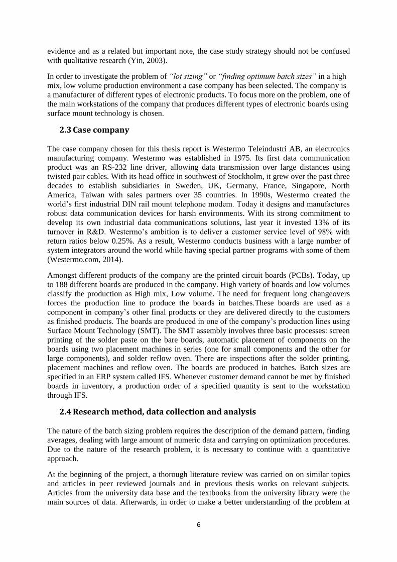
In order to investigate the problem of “lot sizing” or “finding optimum batch sizes” in a high

mix, low volume production environment a case company has been selected. The company is

a manufacturer of different types of electronic products. To focus more on the problem, one of

the main workstations of the company that produces different types of electronic boards using

surface mount technology is chosen.

2.3 Case company

The case company chosen for this thesis report is Westermo Teleindustri AB, an electronics

manufacturing company. Westermo was established in 1975. Its first data communication

product was an RS-232 line driver, allowing data transmission over large distances using

twisted pair cables. With its head office in southwest of Stockholm, it grew over the past three

decades to establish subsidiaries in Sweden, UK, Germany, France, Singapore, North

America, Taiwan with sales partners over 35 countries. In 1990s, Westermo created the

world’s first industrial DIN rail mount telephone modem. Today it designs and manufactures

robust data communication devices for harsh environments. With its strong commitment to

develop its own industrial data communications solutions, last year it invested 13% of its

turnover in R&D. Westermo’s ambition is to deliver a customer service level of 98% with

return ratios below 0.25%. As a result, Westermo conducts business with a large number of

system integrators around the world while having special partner programs with some of them

(Westermo.com, 2014).

Amongst different products of the company are the printed circuit boards (PCBs). Today, up

to 188 different boards are produced in the company. High variety of boards and low volumes

classify the production as High mix, Low volume. The need for frequent long changeovers

forces the production line to produce the boards in batches.These boards are used as a

component in company’s other final products or they are delivered directly to the customers

as finished products. The boards are produced in one of the company’s production lines using

Surface Mount Technology (SMT). The SMT assembly involves three basic processes: screen

printing of the solder paste on the bare boards, automatic placement of components on the

boards using two placement machines in series (one for small components and the other for

large components), and solder reflow oven. There are inspections after the solder printing,

placement machines and reflow oven. The boards are produced in batches. Batch sizes are

specified in an ERP system called IFS. Whenever customer demand cannot be met by finished

boards in inventory, a production order of a specified quantity is sent to the workstation

through IFS.

2.4 Research method, data collection and analysis

The nature of the batch sizing problem requires the description of the demand pattern, finding

averages, dealing with large amount of numeric data and carrying on optimization procedures.

Due to the nature of the research problem, it is necessary to continue with a quantitative

approach.

At the beginning of the project, a thorough literature review was carried on on similar topics

and articles in peer reviewed journals and in previous thesis works on relevant subjects.

Articles from the university data base and the textbooks from the university library were the

main sources of data. Afterwards, in order to make a better understanding of the problem at

7

hand in detail levels, an investigation of the production process was performed through daily

visits of the SMT line, making close observations, asking questions from operators and the

production manager and searching relevant data through company’s data base.

The data required to solve the research problem was collected from company’s ERP system.

This data includes information related to demand patterns for each board, prices, production

quantities, cycle times, capacity and etc. The data from ERP system was in raw form and had

to be processed before turning into meaningful information, therefore a great deal of time was

spent on processing and manipulation of raw data using Excel. To continue, an optimization

model was created which enabled this data to be used. The model was used not only for

calculating the optimum batch sizes, but also to perform capacity analysis and investigating

the effect of setup time reduction on both batch sizes and capacity.

8

3. Theoretic framework

In this chapter, the theoretic framework of this report is explained. Relevant theories are

described and later used in the empirical part.

3.1 Description of an SMT line

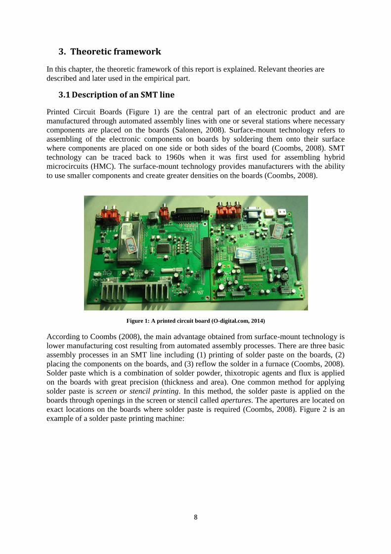
Printed Circuit Boards (Figure 1) are the central part of an electronic product and are

manufactured through automated assembly lines with one or several stations where necessary

components are placed on the boards (Salonen, 2008). Surface-mount technology refers to

assembling of the electronic components on boards by soldering them onto their surface

where components are placed on one side or both sides of the board (Coombs, 2008). SMT

technology can be traced back to 1960s when it was first used for assembling hybrid

microcircuits (HMC). The surface-mount technology provides manufacturers with the ability

to use smaller components and create greater densities on the boards (Coombs, 2008).

Figure 1: A printed circuit board (O-digital.com, 2014)

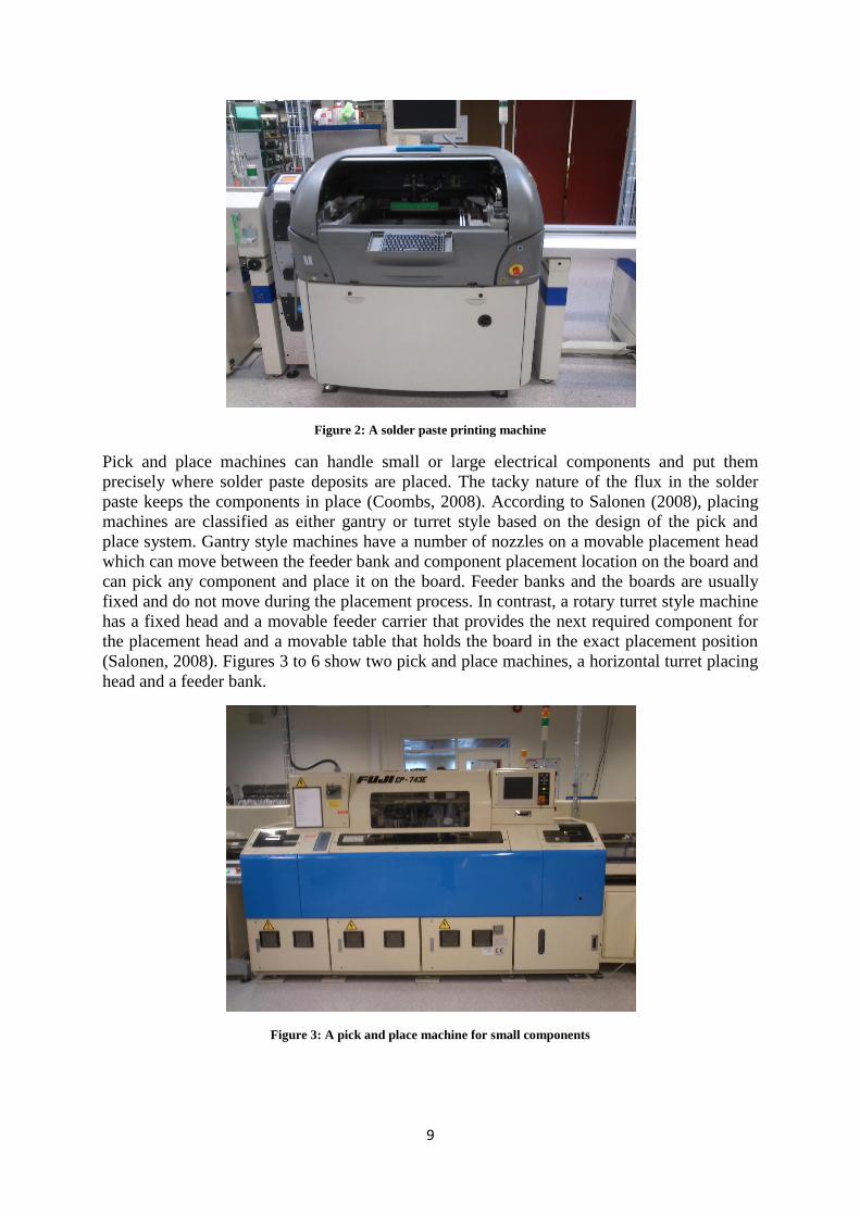
According to Coombs (2008), the main advantage obtained from surface-mount technology is

lower manufacturing cost resulting from automated assembly processes. There are three basic

assembly processes in an SMT line including (1) printing of solder paste on the boards, (2)

placing the components on the boards, and (3) reflow the solder in a furnace (Coombs, 2008).

Solder paste which is a combination of solder powder, thixotropic agents and flux is applied

on the boards with great precision (thickness and area). One common method for applying

solder paste is screen or stencil printing. In this method, the solder paste is applied on the

boards through openings in the screen or stencil called apertures. The apertures are located on

exact locations on the boards where solder paste is required (Coombs, 2008). Figure 2 is an

example of a solder paste printing machine:

9

Figure 2: A solder paste printing machine

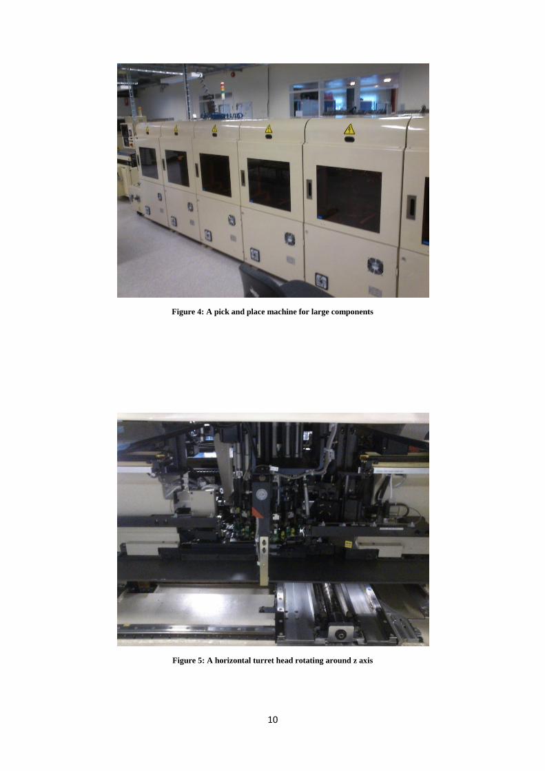
Pick and place machines can handle small or large electrical components and put them

precisely where solder paste deposits are placed. The tacky nature of the flux in the solder

paste keeps the components in place (Coombs, 2008). According to Salonen (2008), placing

machines are classified as either gantry or turret style based on the design of the pick and

place system. Gantry style machines have a number of nozzles on a movable placement head

which can move between the feeder bank and component placement location on the board and

can pick any component and place it on the board. Feeder banks and the boards are usually

fixed and do not move during the placement process. In contrast, a rotary turret style machine

has a fixed head and a movable feeder carrier that provides the next required component for

the placement head and a movable table that holds the board in the exact placement position

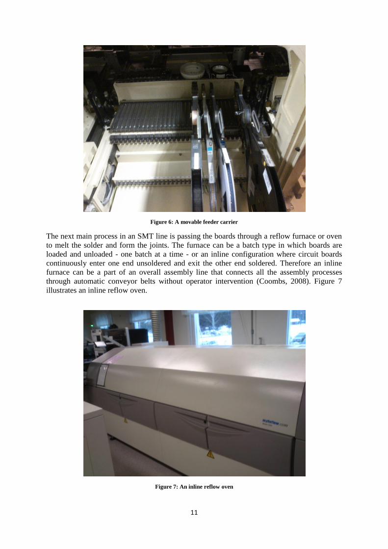
(Salonen, 2008). Figures 3 to 6 show two pick and place machines, a horizontal turret placing

head and a feeder bank.

Figure 3: A pick and place machine for small components

10

Figure 4: A pick and place machine for large components

Figure 5: A horizontal turret head rotating around z axis

11

Figure 6: A movable feeder carrier

The next main process in an SMT line is passing the boards through a reflow furnace or oven

to melt the solder and form the joints. The furnace can be a batch type in which boards are

loaded and unloaded - one batch at a time - or an inline configuration where circuit boards

continuously enter one end unsoldered and exit the other end soldered. Therefore an inline

furnace can be a part of an overall assembly line that connects all the assembly processes

through automatic conveyor belts without operator intervention (Coombs, 2008). Figure 7

illustrates an inline reflow oven.

Figure 7: An inline reflow oven

12

3.2 Economic Order Quantity

Manufacturing companies face conflicting pressures to keep inventory level low enough to

reduce inventory holding costs but at the same time high enough to avoid excess ordering or

setup costs. A good starting point to balance out these two conflicting costs and to determine

the best inventory level or production lot size is to find the economic order quantity (EOQ),

which is a lot size that minimizes the sum of total annual inventory holding costs and setup

costs (Krajewski, Ritzman and Malhotra, 2007). According to Krajewski, Ritzman and

Malhotra (2007) there are a set of assumptions that should be considered before calculating

the EOQ:

1. The demand rate is constant and is known for certain.

2. No constraint is set for lot sizes (such as material handling limitations).

3. Inventory holding cost and setup cost are the only two relevant costs.

4. Decision for each item can be made independently from other items.

5. The lead time is constant and the ordered amount arrives at once rather gradually.

The EOQ is optimal when all the assumptions above are satisfied. However, there are few

examples in reality where the situation is that simple. Nonetheless, the EOQ is still a

reasonable approximation of the optimum lot size even when several of the assumptions

above are not met (Krajewski, Ritzman and Malhotra, 2007).

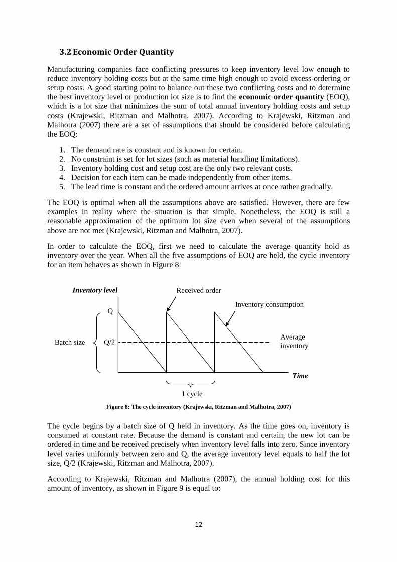
In order to calculate the EOQ, first we need to calculate the average quantity hold as

inventory over the year. When all the five assumptions of EOQ are held, the cycle inventory

for an item behaves as shown in Figure 8:

The cycle begins by a batch size of Q held in inventory. As the time goes on, inventory is

consumed at constant rate. Because the demand is constant and certain, the new lot can be

ordered in time and be received precisely when inventory level falls into zero. Since inventory

level varies uniformly between zero and Q, the average inventory level equals to half the lot

size, Q/2 (Krajewski, Ritzman and Malhotra, 2007).

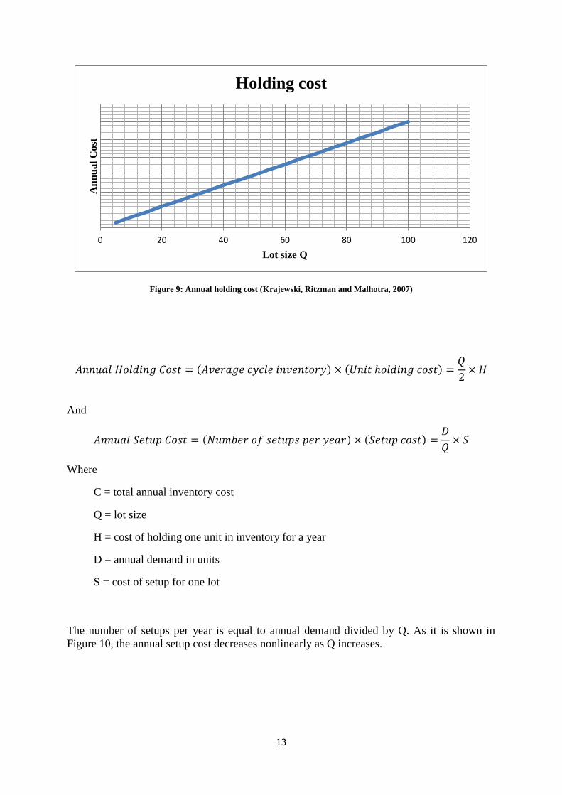
According to Krajewski, Ritzman and Malhotra (2007), the annual holding cost for this

amount of inventory, as shown in Figure 9 is equal to:

Average

inventory

1 cycle

Q

Q/2

Received order

Inventory consumption

Batch size

Inventory level

Time

Figure 8: The cycle inventory (Krajewski, Ritzman and Malhotra, 2007)

13

Figure 9: Annual holding cost (Krajewski, Ritzman and Malhotra, 2007)

( ) ( )

And

( ) ( )

Where

C = total annual inventory cost

Q = lot size

H = cost of holding one unit in inventory for a year

D = annual demand in units

S = cost of setup for one lot

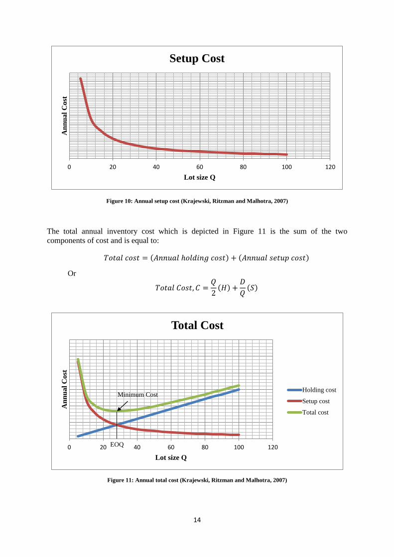
The number of setups per year is equal to annual demand divided by Q. As it is shown in

Figure 10, the annual setup cost decreases nonlinearly as Q increases.

0 20 40 60 80 100 120

An

nu

al

Co

st

Lot size Q

Holding cost

14

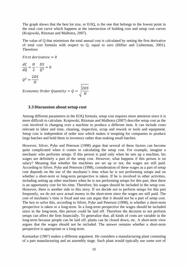
Figure 10: Annual setup cost (Krajewski, Ritzman and Malhotra, 2007)

The total annual inventory cost which is depicted in Figure 11 is the sum of the two

components of cost and is equal to:

( ) ( )

Or

( )

( )

Figure 11: Annual total cost (Krajewski, Ritzman and Malhotra, 2007)

0 20 40 60 80 100 120

An

nu

al

Co

st

Lot size Q

Setup Cost

0 20 40 60 80 100 120

An

nu

al

Cost

Lot size Q

Total Cost

Holding cost

Setup cost

Total cost

Minimum Cost

EOQ

15

The graph shows that the best lot size, or EOQ, is the one that belongs to the lowest point in

the total cost curve which happens at the intersection of holding cost and setup cost curves

(Krajewski, Ritzman and Malhotra, 2007).

The value of Q that minimizes the total annual cost is calculated by setting the first derivative

of total cost formula with respect to Q, equal to zero (Hillier and Lieberman, 2001).

Therefore:

√

3.3 Discussion about setup cost

Among different parameters in the EOQ formula, setup cost requires more attention since it is

more difficult to calculate. Krajewski, Ritzman and Malhotra (2007) describe setup cost as the

cost involved in changing over a machine to produce a different item. It can include costs

relevant to labor and time, cleaning, inspection, scrap and rework or tools and equipment.

Setup cost is independent of order size which makes it tempting for companies to produce

large batches and hold them in inventory rather than making small batches.

However, Silver, Pyke and Peterson (1998) argue that several of these factors can become

quite complicated when it comes to calculating the setup cost. For example, imagine a

mechanic who performs setups. If this person is paid only when he sets up a machine, his

wages are definitely a part of the setup cost. However, what happens if this person is on

salary? Meaning that whether the machines are set up or not, the wages are still paid.

According to Silver, Pyke and Peterson (1998), consideration of these wages as a part of setup

cost depends on the use of the mechanic’s time when he is not performing setups and on

whether a short-term or long-term perspective is taken. If he is involved in other activities,

including setting up other machines when he is not performing setups for this part, then there

is an opportunity cost for his time. Therefore, his wages should be included in the setup cost.

However, there is another side to this story. If we decide not to perform setups for this part

frequently, we do not save actual money in the short-term since the wages are still paid. The

cost of mechanic’s time is fixed and one can argue that it should not be a part of setup cost.

The key to solve this, according to Silver, Pyke and Peterson (1998), is whether a short-term

perspective is taken or a long-term. In a long-term perspective the wages should be included

since in the long-term, this person could be laid off. Therefore the decision to not perform

setups can affect the firm financially. To generalize that, all kinds of costs are variable in the

long-term because people can be laid off, plants can be closed down, etc. A short-term view

argues that the wages should not be included. The answer remains whether a short-term

perspective is appropriate or a long-term.

Karmarkar (1987) makes a different argument. He considers a manufacturing plant consisting

of a part manufacturing and an assembly stage. Such plant would typically use some sort of

16

MRP system to determine parts’ demands (which is usually lumpy), bill-of-materials,

production times, lead times, waiting times and batch sizes. There is a sizable literature on

this area that studies lot-sizing under these dynamic conditions and develops models that

consider capacity constraints, multiple items or multiple stages. All these models try to make

a tradeoff between productivity losses from making too many small batches and opportunity

costs of tying up too much capital in inventory as large batches. These costs are represented

by fixed setup costs and variable inventory holding costs respectively. This representation of

cost, although common, fails to capture the nature of the batching problem. In reality, there is

often no real setup cost with respect to cash flows being affected. Setup costs are rather a

surrogate for violation of capacity constraints. Therefore, the idea of a fixed setup cost,

independent of the solution, is quite misleading since it is rather a consequence of the

solution. There are real setup costs in terms of material consumption but they should be

distinguished from opportunity costs caused by lost production capacity (Karmarkar, 1987).

Finally, one can spend months to nail the exact value of the setup cost precisely, but it is more

useful to change the condition of the processes that determine the value of the setup cost, in

order to actually reduce it (Silver, Pyke and Peterson, 1998). Single Minute Exchange of Die

(SMED) is a renowned theory in lean manufacturing that deals with this issue.

3.4 Single Minute Exchange of Die

Many manufacturing companies consider High mix, Low volume production as their single

greatest challenge. However, at any rate, problem facing companies is not High mix, Low

volume production but production involving frequent setups and small lot sizes. SMED

system, also known as Single-minute setup, refers to theory and techniques for performing

setup operations under ten minutes, i.e., a number of minutes that can be expressed in a single

digit. Although not every setup operation can be performed in single-digit minutes, this is the

goal of the system and can be met in surprisingly high percentage of cases. Even when it

cannot, drastic reductions in setup times are usually possible. SMED was later adopted by all

Toyota plants and became one of the core elements of Toyota Production System (Shingo,

1985).

According to Shingo (1985), setup operations have traditionally demanded a great amount of

time and have caused a great deal of inefficiencies in manufacturing companies. Increasing lot

sizes was a solution found to this problem. If lot sizes are increased, the ratio of setup time

over the number of operations is greatly reduced (Table 1):

Table 1: Relationship between setup time and lot size (Shingo, 1985)

Setup

Time

Lot

Size

Principal

Operation Time

Per Item

Operation Time Ratio

(%)

Ratio

(%)

4 hrs. 100 1 min.

100

4 hrs. 1000 1 min.

36 100

4 hrs. 10000 1 min.

30 83

17

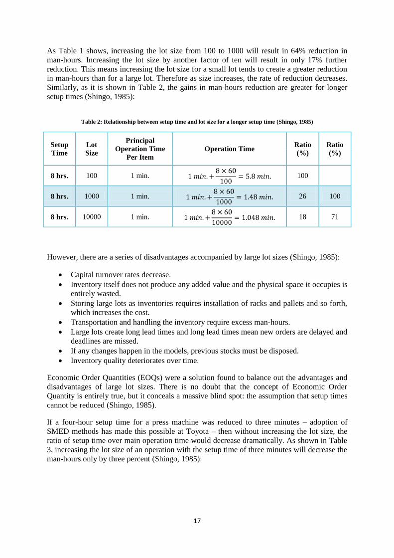
As Table 1 shows, increasing the lot size from 100 to 1000 will result in 64% reduction in

man-hours. Increasing the lot size by another factor of ten will result in only 17% further

reduction. This means increasing the lot size for a small lot tends to create a greater reduction

in man-hours than for a large lot. Therefore as size increases, the rate of reduction decreases.

Similarly, as it is shown in Table 2, the gains in man-hours reduction are greater for longer

setup times (Shingo, 1985):

Table 2: Relationship between setup time and lot size for a longer setup time (Shingo, 1985)

Setup

Time

Lot

Size

Principal

Operation Time

Per Item

Operation Time Ratio

(%)

Ratio

(%)

8 hrs. 100 1 min.

100

8 hrs. 1000 1 min.

26 100

8 hrs. 10000 1 min.

18 71

However, there are a series of disadvantages accompanied by large lot sizes (Shingo, 1985):

Capital turnover rates decrease.

Inventory itself does not produce any added value and the physical space it occupies is

entirely wasted.

Storing large lots as inventories requires installation of racks and pallets and so forth,

which increases the cost.

Transportation and handling the inventory require excess man-hours.

Large lots create long lead times and long lead times mean new orders are delayed and

deadlines are missed.

If any changes happen in the models, previous stocks must be disposed.

Inventory quality deteriorates over time.

Economic Order Quantities (EOQs) were a solution found to balance out the advantages and

disadvantages of large lot sizes. There is no doubt that the concept of Economic Order

Quantity is entirely true, but it conceals a massive blind spot: the assumption that setup times

cannot be reduced (Shingo, 1985).

If a four-hour setup time for a press machine was reduced to three minutes – adoption of

SMED methods has made this possible at Toyota – then without increasing the lot size, the

ratio of setup time over main operation time would decrease dramatically. As shown in Table

3, increasing the lot size of an operation with the setup time of three minutes will decrease the

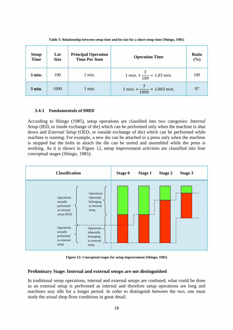
man-hours only by three percent (Shingo, 1985):

18

Table 3: Relationship between setup time and lot size for a short setup time (Shingo, 1985)

Setup

Time

Lot

Size

Principal Operation

Time Per Item Operation Time

Ratio

(%)

3 min. 100 1 min.

100

3 min. 1000 1 min.

97

3.4.1 Fundamentals of SMED

According to Shingo (1985), setup operations are classified into two categories: Internal

Setup (IED, or inside exchange of die) which can be performed only when the machine is shut

down and External Setup (OED, or outside exchange of die) which can be performed while

machine is running. For example, a new die can be attached to a press only when the machine

is stopped but the bolts to attach the die can be sorted and assembled while the press is

working. As it is shown in Figure 12, setup improvement activities are classified into four

conceptual stages (Shingo, 1985):

Classification Stage 0 Stage 1 Stage 2 Stage 3

Figure 12: Conceptual stages for setup improvement (Shingo, 1985)

Preliminary Stage: Internal and external setups are not distinguished

In traditional setup operations, internal and external setups are confused; what could be done

as an external setup is performed as internal and therefore setup operations are long and

machines stay idle for a longer period. In order to distinguish between the two, one must

study the actual shop floor conditions in great detail.

Operations

inherently

belonging

to internal

setup

Operations

inherently

belonging

to external

setup

Operations

actually

performed

as internal

setup (IED)

Operations

actually

performed

as external

setup

(OED)

19

Stage 1: Separating internal and external setup

The most important step in implementing SMED is distinguishing between these two.

Mastering this distinction is the passport towards SMED goal.

Stage 2: Converting internal setup to external

Distinguishing between internal and external setup activities alone can result in significant

setup time reduction in some cases. However, this is still insufficient to achieve SMED

objective. The second stage involves two important notions:

Re-examining the operations to see if any step is wrongly assumed to be internal

Finding ways to convert these steps to external setup activity

An example could be preheating some elements that have previously been heated only when

setup starts or converting centering to an external operation by doing it before the production

begins.

Stage 3: Streamlining all aspects of setup operation

Although the single-minute goal can be achieved by converting to external setup in many

occasions, this is not true in majority of cases. Therefore one must make a strong effort in

streamlining all elements of internal and external setup. Therefore, stage 3 requires detailed

analysis of each element of setup operations. Parallel operations involving more than one

operator can be very helpful in speeding up this kind of work. For example, an internal

operation that takes 12 minutes by one operator can be performed in less than 6 minutes in

many cases by involving two operators, thanks to the economies of movements.

3.4.2 Discussion over SMED

Despite the many arguments for setup time reductions in the existing literature, the issue of

justifying investments on setup reductions and optimally allocating finite resources has to a

large extent been glossed over (Nye, Jewkes and Dilts, 2001). For example, one of the main

objectives of SMED system is to reduce setup times to less than 10 minutes (Shingo, 1985),

without offering any reason for this particular target, nor mentioning what target is

appropriate in many cases where setup times cannot be reduced to less than 10 minutes (Nye,

Jewkes and Dilts, 2001). The philosophy that companies should strive for zero setup times is

laudable, but it may not be a realistic objective. For example, a manufacturer of N different

products can achieve zero setup time by allocating N parallel production systems. Clearly, N

does not need to be very large before the cost of investments to reach zero setups far exceeds

any potential economic advantages (Nye, Jewkes and Dilts, 2001).

However, it is clear that flexibility is strongly linked with small lot sizes. The smaller the lot

sizes are, the easier it is for a manufacturing company to react to changes in the market

demand (Sherali, Goubergen and Landeghem, 2008). Goubergen and Landeghem (2002)

describe three reasons why short setups are appropriate for any company:

Companies need to be flexible. Flexibility requires small lot sizes and small lot sizes

need short setups.

Setups need to be reduced to maximize the capacity and reduce the bottlenecks.

Short setups increase machine performance and OEE and therefore decrease

production cost.

20

Ferradás and Salonitis (2013) argue that although SMED is known for about twenty five

years and has been implemented successfully in many companies, a number of plants have

failed to implement it. One reason is that some companies put too much attention on

transferring internal activities to external activities, missing the importance of streamlining

both activities by design improvements (Ferradás and Salonitis, 2013). Gest, et al. (1995) say

that the main reason some companies fail in SMED implementation is that they lack structure

and focus. It is not uncommon for a SMED project to lose momentum and wither away after a

while. In many cases, the SMED improvements have been through shop floor kaizen-based

initiatives and early gains have reverted back to previous levels once the management focus

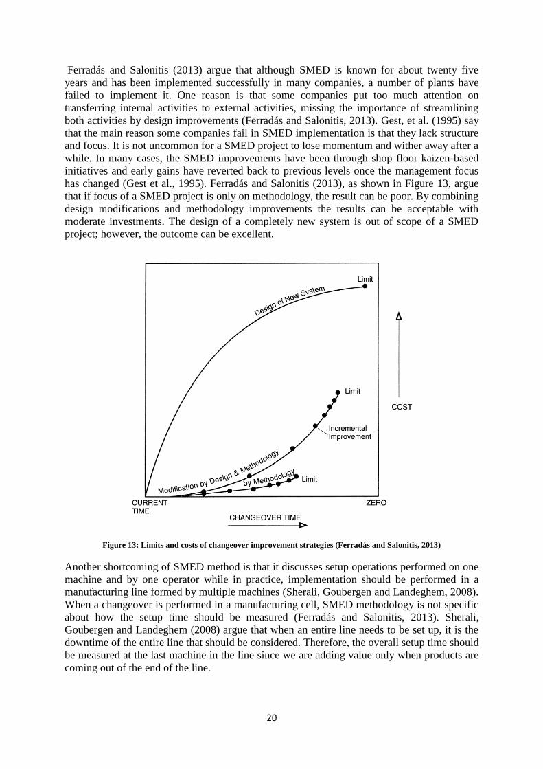
has changed (Gest et al., 1995). Ferradás and Salonitis (2013), as shown in Figure 13, argue

that if focus of a SMED project is only on methodology, the result can be poor. By combining

design modifications and methodology improvements the results can be acceptable with

moderate investments. The design of a completely new system is out of scope of a SMED

project; however, the outcome can be excellent.

Figure 13: Limits and costs of changeover improvement strategies (Ferradás and Salonitis, 2013)

Another shortcoming of SMED method is that it discusses setup operations performed on one

machine and by one operator while in practice, implementation should be performed in a

manufacturing line formed by multiple machines (Sherali, Goubergen and Landeghem, 2008).

When a changeover is performed in a manufacturing cell, SMED methodology is not specific

about how the setup time should be measured (Ferradás and Salonitis, 2013). Sherali,

Goubergen and Landeghem (2008) argue that when an entire line needs to be set up, it is the

downtime of the entire line that should be considered. Therefore, the overall setup time should

be measured at the last machine in the line since we are adding value only when products are

coming out of the end of the line.

21

3.5 Linear optimization, nonlinear optimization

Another technique that can be used to find optimum batch sizes is Operations Research (OR).

OR is a field that uses mathematical programming to find optimum values of an optimization

problem. Linear programming (LP) is the most basic mathematical programming. LP refers to

an optimization problem where both objective function and constraints are linear (Pinedo,

2005). According to Pinedo (2005), an LP can be expressed as follows:

Subject to

The vector is referred to as cost vector. The objective of the LP is to minimize the

cost by determining the optimum value of variables . The Column vector

is called activity vector. The value of the variable refers to the level at which

the activity i is performed. The vector is called the resource vector and

determines the resource limitations (Pinedo, 2005).

The main assumption of LP is that all of its functions - objective function or constraint

functions - are linear. Although for many cases and examples this assumption applies, there

are numerous cases where linearity assumption does not hold. For example, economists agree

that some degree of nonlinearity is a rule not an exception in their economic planning

problems (Hillier and Lieberman, 2001). A nonlinear programming (NLP) is a generalization

of linear programming which allows the objective function or the constraints to be nonlinear

(Pinedo, 2005).

3.6 Exact methods, Heuristics

In order to solve an OR problem one needs to implement a proper optimization algorithm. In

general there are two classes of optimization algorithms: exact methods and heuristic

methods. Exact methods try to find a global optimal solution to the problem no matter how

long it takes. Heuristics try to find a near optimal answer in a short time. Exact methods use

mathematical methods to guarantee that their solutions are optimal. They can be efficient for

problems with small or medium size but they require large amount of time for problems with

larger size. Heuristics, however, are algorithms based on rules of thumb or common sense, or

refinements of exact methods (Rader, 2010).

Exact methods may have to examine every feasible solution before confirming optimality.

Therefore, for many problems concerning the real world, exact methods can be very time

consuming. Besides, those who are interested in solving the real world problems often do not

have the time for guaranteed optimality when a reasonable solution will suffice. In these

.

.

.

22

cases, heuristic methods are often used (Rader, 2010). For instance, from 2003 to 2004 a

group of researchers tried to find the optimal tour through 24978 cities, towns and villages in

Sweden. This is an example of famous traveling salesperson problem that has been studied for

years by operations researchers. The optimal tour was obtained using heuristic methods within

a few hours of CPU time and it was later confirmed to be optimal after 84.4 CPU years –

exact algorithm was run in parallel in a series of workstations – (Rader, 2010).

3.6.1 Genetic Algorithm

Genetic Algorithm (GA) is one of the most famous and widely used heuristic algorithms. GA

is a heuristic method that solves large constrained and unconstrained optimization problems

by using a process that mimics natural selection in biological evolution. The algorithm works

by repeatedly modifying a population of candidate solutions. At each iteration, the algorithm

selects individuals from the current population and uses them as parents to create the next

generation. Over successive generations, the population evolves towards a better optimal

solution (Mathworks.se, 2014). Genetic algorithm is highly suited for optimization problems

where standard algorithms cannot be applied easily. This includes problems where objective

function or constraints are discontinuous, non-differentiable, stochastic or highly nonlinear

(Mathworks.se, 2014).

Genetic algorithm is different from other classical heuristics in two main ways

(Mathworks.se, 2014):

1) The classical algorithms create a single point at each iteration and the sequence of

single points moves towards an optimal solution while GA produces a population of

points at each iteration and the best point in the population approaches the optimal

solution.

2) Classical algorithms create each successive point using deterministic computation

while GA computes successive generations using random number generators.

The following procedure describes how genetic algorithm works (Mathworks.se, 2014):

1) The algorithm begins by creating an initial population using random numbers.

2) The algorithm starts to generate a sequence of populations. In order to create the next

generation, the algorithm uses the individuals in the current population by performing

the following steps:

a) Rates each member of the current population by evaluating its fitness

value

b) Scales the scored values to turn them into more usable set of values

c) Selects individuals, called parents, based on their fitness value

d) Some of the individuals with the best fitness value are chosen as elites.

These elites pass to the next generation.

e) From the parents, children are produced. Children are produced either

by crossover or by mutation.

f) Children replace the current population and form the next generation

3) The algorithm stops, when one of the stopping criteria is met.

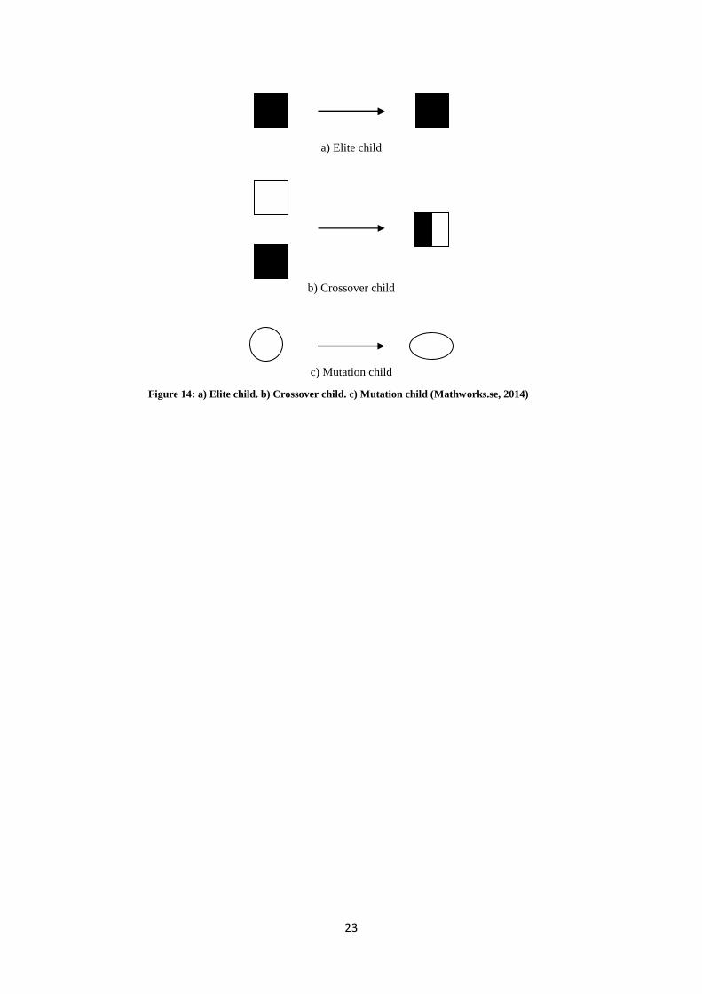
The process of mutation and crossover are depicted in Figure 14:

23

a) Elite child

b) Crossover child

c) Mutation child

Figure 14: a) Elite child. b) Crossover child. c) Mutation child (Mathworks.se, 2014)

24

4. Results (Empirics)

In this chapter, empirical results are presented. The EOQs are calculated for the boards

followed by a discussion over setup cost. Then, an optimization model is presented for

solving the problem and results are illustrated with tables and figures.

4.1 Calculating EOQs

Through IFS system, one can find the current batch sizes used for different boards. In order to

find the optimum batches for each board, the first idea was to calculate the EOQs for every

board and compare them with the current batch sizes to get a general idea of the current

situation. According to EOQ formula√

, there are three parameters that need to be

identified for each board to calculate the economic order quantity: D, representing the annual

demand for each board; S, representing the setup cost for each board and H, representing the

annual inventory holding cost for each board. The annual demands for boards are obtainable

through IFS. Every demand or production order is recorded in the system by the date of order

and is transferable to an excel file. Through the excel file, the total demand for each board can

be calculated. The time span for the orders was chosen as first day of January to last day of

December 2013. This way, there is no need to rely on this year forecasts and recent historical

data can be used. After calculating annual demands, inventory holding costs should be

defined. Based on information from the financial department, the annual inventory cost is 10

percent of the inventory value of the boards. The price of each board is accessible through

IFS. By multiplying this price with 0.1 – the inventory holding rate – the annual holding cost

can be obtained. The last parameter to define is the setup cost. According to the company’s

financial department, setup costs are consisted of three parts. The employee’s salary, the

overhead cost for the whole factory and the overhead cost for the SMT workstation with

values 1190 SEK, 716 SEK and 414 SEK per hour respectively and the total cost of 2320

SEK. The logic behind it is that this is the cost that company has to bear. When setups are

performed, no value added activity is performed to cover these costs and therefore they are

considered as setup cost. The average setup time is about 22 minutes or 0.36 hr based on IFS

data. Although this number is not accurate and setup durations differ for each board, but it is a

good approximation of the average time spent for changing over the machines from one board

to another. The setup cost therefore will be this time presented in hour, multiplied by the

hourly setup cost. The results of these calculations are presented in Table 4.

The boards are represented by Xi in the table below. Minimum lot sizes are the current batch

sizes used for production. They refer to the amount that should be produced if the demand

cannot be met by the existing boards in inventory. For example, for a minimum lot size of 30,

if the inventory level for that particular board is 15 units and the demand is 20, a production

order of 30 will be issued to meet the demand. The new inventory level will be 15 + 30 – 20 =

25. However if the demand is even more, for example 55, a lot size of 30 cannot satisfy the

demand. In order to meet this large demand, a production order of 55 – 15 = 40 will be issued.

Some of the boards – which usually have low demand and high price – are produced only

based on customer order quantity, meaning that if the customer wants a batch of 25, a batch of

25 will be produced and delivered. Some other boards are prototypes and are not produced

regularly. These boards, all together, have a minimum lot size of zero, indicating that there are

produced only when there is a demand for them.

25

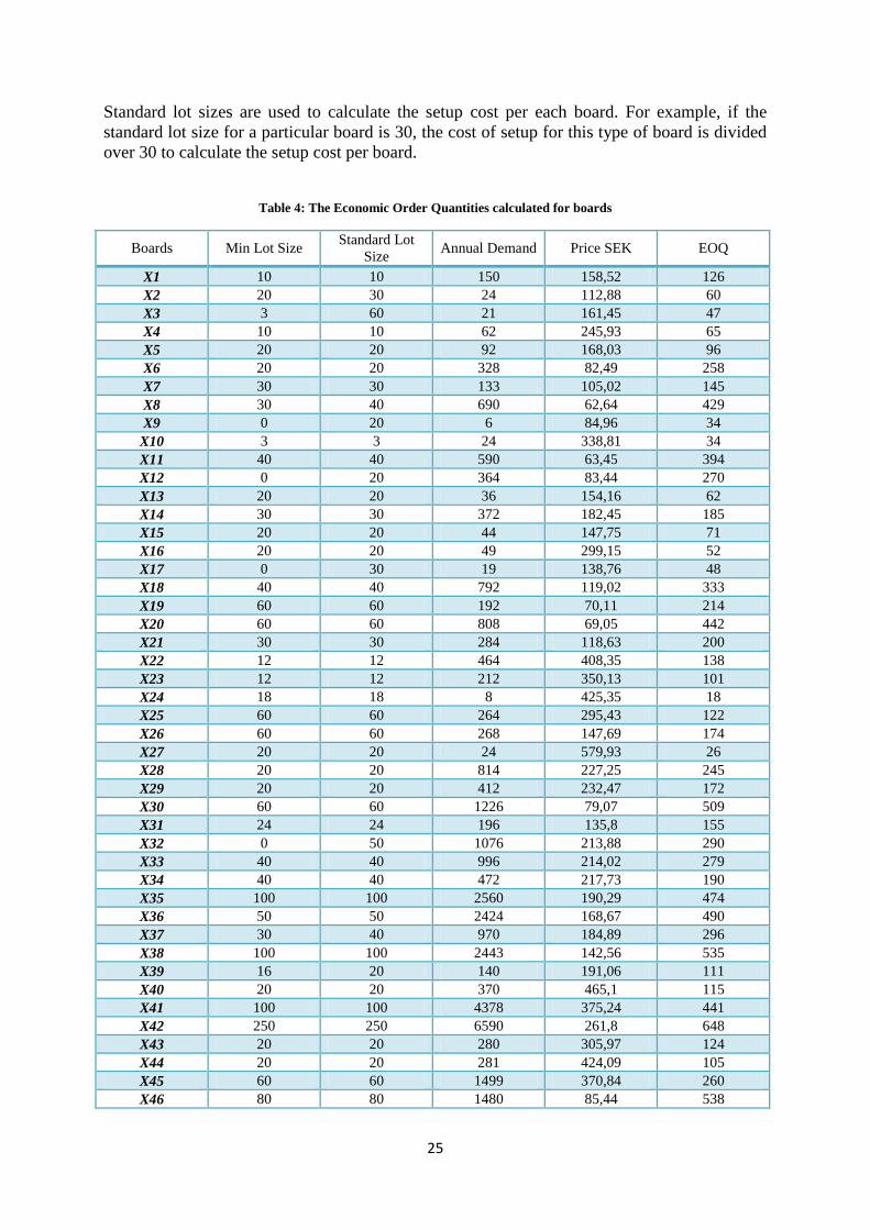
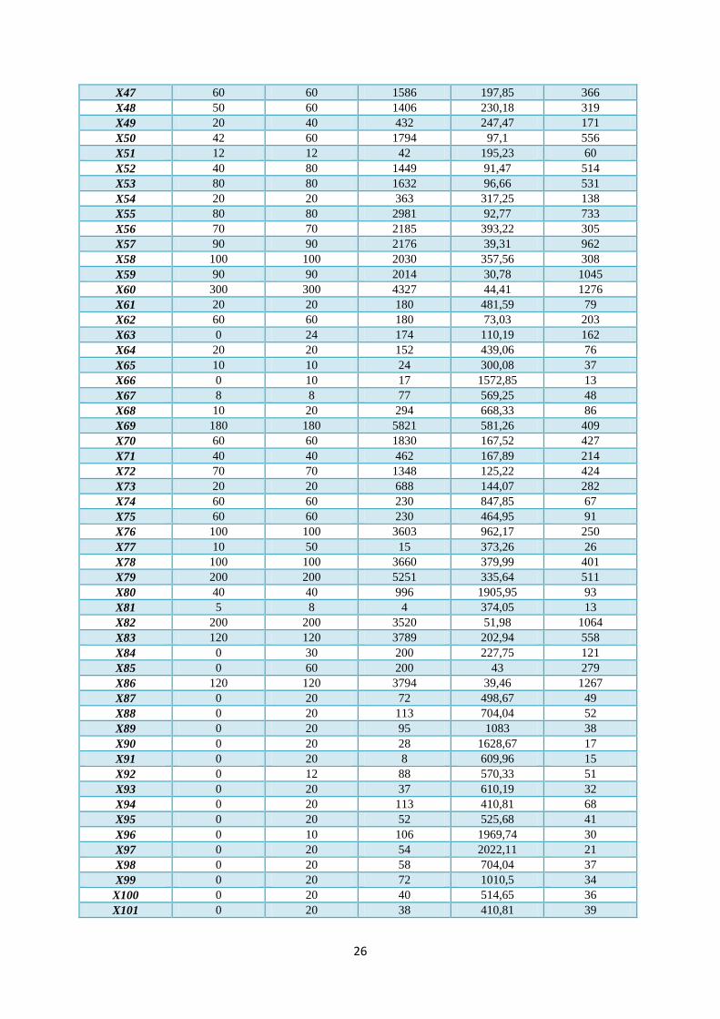
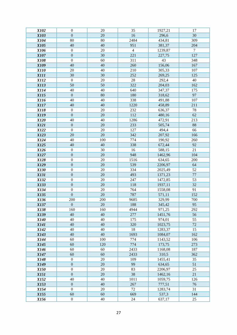
Standard lot sizes are used to calculate the setup cost per each board. For example, if the

standard lot size for a particular board is 30, the cost of setup for this type of board is divided

over 30 to calculate the setup cost per board.

Table 4: The Economic Order Quantities calculated for boards

Boards Min Lot Size Standard Lot

Size Annual Demand Price SEK EOQ

X1 10 10 150 158,52 126

X2 20 30 24 112,88 60

X3 3 60 21 161,45 47

X4 10 10 62 245,93 65

X5 20 20 92 168,03 96

X6 20 20 328 82,49 258

X7 30 30 133 105,02 145

X8 30 40 690 62,64 429

X9 0 20 6 84,96 34

X10 3 3 24 338,81 34

X11 40 40 590 63,45 394

X12 0 20 364 83,44 270

X13 20 20 36 154,16 62

X14 30 30 372 182,45 185

X15 20 20 44 147,75 71

X16 20 20 49 299,15 52

X17 0 30 19 138,76 48

X18 40 40 792 119,02 333

X19 60 60 192 70,11 214

X20 60 60 808 69,05 442

X21 30 30 284 118,63 200

X22 12 12 464 408,35 138

X23 12 12 212 350,13 101

X24 18 18 8 425,35 18

X25 60 60 264 295,43 122

X26 60 60 268 147,69 174

X27 20 20 24 579,93 26

X28 20 20 814 227,25 245

X29 20 20 412 232,47 172

X30 60 60 1226 79,07 509

X31 24 24 196 135,8 155

X32 0 50 1076 213,88 290

X33 40 40 996 214,02 279

X34 40 40 472 217,73 190

X35 100 100 2560 190,29 474

X36 50 50 2424 168,67 490

X37 30 40 970 184,89 296

X38 100 100 2443 142,56 535

X39 16 20 140 191,06 111

X40 20 20 370 465,1 115

X41 100 100 4378 375,24 441

X42 250 250 6590 261,8 648

X43 20 20 280 305,97 124

X44 20 20 281 424,09 105

X45 60 60 1499 370,84 260

X46 80 80 1480 85,44 538

26

X47 60 60 1586 197,85 366

X48 50 60 1406 230,18 319

X49 20 40 432 247,47 171

X50 42 60 1794 97,1 556

X51 12 12 42 195,23 60

X52 40 80 1449 91,47 514

X53 80 80 1632 96,66 531

X54 20 20 363 317,25 138

X55 80 80 2981 92,77 733

X56 70 70 2185 393,22 305

X57 90 90 2176 39,31 962

X58 100 100 2030 357,56 308

X59 90 90 2014 30,78 1045

X60 300 300 4327 44,41 1276

X61 20 20 180 481,59 79

X62 60 60 180 73,03 203

X63 0 24 174 110,19 162

X64 20 20 152 439,06 76

X65 10 10 24 300,08 37

X66 0 10 17 1572,85 13

X67 8 8 77 569,25 48

X68 10 20 294 668,33 86

X69 180 180 5821 581,26 409

X70 60 60 1830 167,52 427

X71 40 40 462 167,89 214

X72 70 70 1348 125,22 424

X73 20 20 688 144,07 282

X74 60 60 230 847,85 67

X75 60 60 230 464,95 91

X76 100 100 3603 962,17 250

X77 10 50 15 373,26 26

X78 100 100 3660 379,99 401

X79 200 200 5251 335,64 511

X80 40 40 996 1905,95 93

X81 5 8 4 374,05 13

X82 200 200 3520 51,98 1064

X83 120 120 3789 202,94 558

X84 0 30 200 227,75 121

X85 0 60 200 43 279

X86 120 120 3794 39,46 1267

X87 0 20 72 498,67 49

X88 0 20 113 704,04 52

X89 0 20 95 1083 38

X90 0 20 28 1628,67 17

X91 0 20 8 609,96 15

X92 0 12 88 570,33 51

X93 0 20 37 610,19 32

X94 0 20 113 410,81 68

X95 0 20 52 525,68 41

X96 0 10 106 1969,74 30

X97 0 20 54 2022,11 21

X98 0 20 58 704,04 37

X99 0 20 72 1010,5 34

X100 0 20 40 514,65 36

X101 0 20 38 410,81 39

27

X102 0 20 35 1927,21 17

X103 0 20 16 296,6 30

X104 80 80 2484 434,81 309

X105 40 40 951 381,37 204

X106 0 20 4 1239,87 7

X107 0 30 221 227,75 127

X108 0 60 311 43 348

X109 40 40 260 156,06 167

X110 20 40 210 305,33 107

X111 30 30 252 269,25 125

X112 0 20 28 292,4 40

X113 50 50 322 204,03 162

X114 40 40 640 347,37 175

X115 0 80 180 318,62 97

X116 40 40 338 491,88 107

X117 40 40 1220 458,89 211

X118 0 20 232 636,37 78

X119 0 20 112 480,16 62

X120 40 40 1286 472,91 213

X121 0 20 233 505,74 88

X122 0 20 127 494,4 66

X123 20 20 342 207,92 166

X124 40 100 774 190,92 260

X125 40 40 338 672,44 92

X126 0 30 16 588,15 21

X127 0 20 948 1462,96 104

X128 0 20 1516 634,65 200

X129 0 20 539 2206,97 64

X130 0 20 334 2025,49 52

X131 0 20 493 1371,23 77

X132 0 20 247 1472,85 53

X133 0 20 118 1937,11 32

X134 0 20 764 1558,08 91

X135 0 20 787 571,11 152

X136 200 200 9685 329,99 700

X137 0 20 188 345,42 95

X138 160 160 4944 971,25 292

X139 40 40 277 1451,76 56

X140 40 40 175 974,01 55

X141 40 40 320 1023,75 72

X142 40 40 18 1283,37 15

X143 40 40 1693 1084,07 162

X144 60 100 774 1143,52 106

X145 60 120 774 173,75 273

X146 60 60 2433 1168,08 187

X147 60 60 2433 310,5 362

X148 0 20 109 1455,41 35

X149 0 20 99 634,65 51

X150 0 20 83 2206,97 25

X151 0 20 38 1462,16 21

X152 40 40 1011 1059,75 126

X153 0 40 267 777,51 76

X154 0 20 72 1283,74 31

X155 60 60 669 537,3 144

X156 0 40 24 637,17 25

28

X157 0 20 69 565,14 45

X158 80 80 2519 472,03 299

X159 40 40 378 271,92 152

X160 0 20 23 650,64 24

X161 0 20 76 534,67 49

X162 20 20 641 891,38 110

X163 20 40 138 811 53

X164 0 20 76 891,38 38

X165 0 20 4 832,26 9

X166 20 20 641 781,26 117

X167 0 20 73 781,26 40

X168 60 60 1648 57,27 693

X169 40 40 372 509,43 110

X170 60 60 1316 477,9 214

X171 20 20 128 864,07 50

X172 20 20 267 711,74 79

X173 20 20 354 1196,4 70

X174 40 40 950 1139,62 118

X175 60 60 623 217,67 219

X176 40 60 676 55,32 452

X177 0 20 68 143,45 89

X178 0 20 75 272,07 68

X179 20 20 382 1087,27 77

X180 0 20 56 1308,66 27

X181 0 20 42 69,5 100

X182 0 20 16 69,5 62

X183 0 80 37 547,55 34

X184 0 40 45 483,92 39

X185 0 20 27 2022,11 15

X186 0 20 44 143,45 72

X187 0 80 59 466,78 46

X188 0 40 12 618,69 18

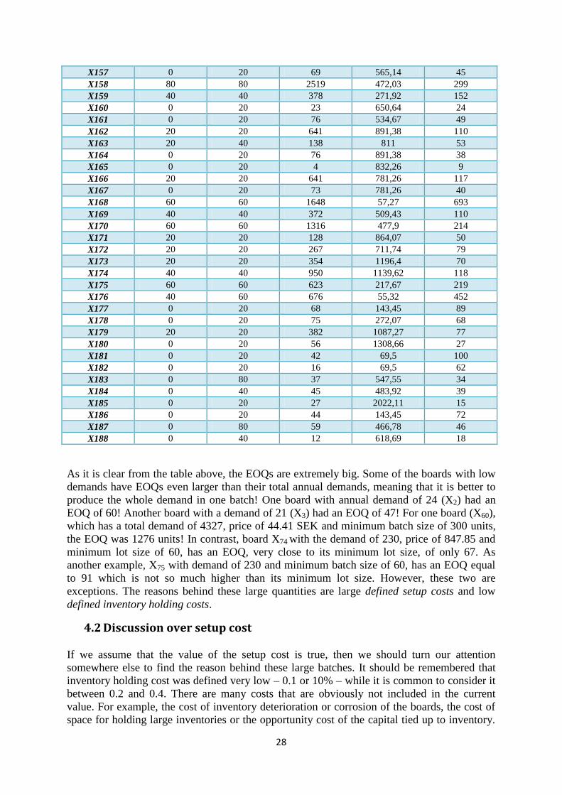
As it is clear from the table above, the EOQs are extremely big. Some of the boards with low

demands have EOQs even larger than their total annual demands, meaning that it is better to

produce the whole demand in one batch! One board with annual demand of 24 (X2) had an

EOQ of 60! Another board with a demand of 21 (X3) had an EOQ of 47! For one board (X60),

which has a total demand of 4327, price of 44.41 SEK and minimum batch size of 300 units,

the EOQ was 1276 units! In contrast, board X74 with the demand of 230, price of 847.85 and

minimum lot size of 60, has an EOQ, very close to its minimum lot size, of only 67. As

another example, X75 with demand of 230 and minimum batch size of 60, has an EOQ equal

to 91 which is not so much higher than its minimum lot size. However, these two are

exceptions. The reasons behind these large quantities are large defined setup costs and low

defined inventory holding costs.

4.2 Discussion over setup cost

If we assume that the value of the setup cost is true, then we should turn our attention

somewhere else to find the reason behind these large batches. It should be remembered that

inventory holding cost was defined very low – 0.1 or 10% – while it is common to consider it

between 0.2 and 0.4. There are many costs that are obviously not included in the current

value. For example, the cost of inventory deterioration or corrosion of the boards, the cost of

space for holding large inventories or the opportunity cost of the capital tied up to inventory.

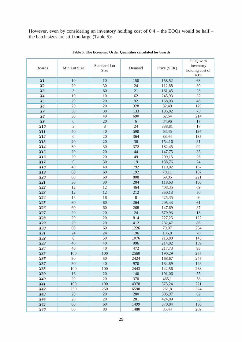
29

However, even by considering an inventory holding cost of 0.4 – the EOQs would be half –

the batch sizes are still too large (Table 5):

Table 5: The Economic Order Quantities calculated for boards

Boards Min Lot Size Standard Lot

Size Demand Price (SEK)

EOQ with

inventory

holding cost of

40%

X1 10 10 150 158,52 63

X2 20 30 24 112,88 30

X3 3 60 21 161,45 23

X4 10 10 62 245,93 32

X5 20 20 92 168,03 48

X6 20 20 328 82,49 129

X7 30 30 133 105,02 73

X8 30 40 690 62,64 214

X9 0 20 6 84,96 17

X10 3 3 24 338,81 17

X11 40 40 590 63,45 197

X12 0 20 364 83,44 135

X13 20 20 36 154,16 31

X14 30 30 372 182,45 92

X15 20 20 44 147,75 35

X16 20 20 49 299,15 26

X17 0 30 19 138,76 24

X18 40 40 792 119,02 167

X19 60 60 192 70,11 107

X20 60 60 808 69,05 221

X21 30 30 284 118,63 100

X22 12 12 464 408,35 69

X23 12 12 212 350,13 50

X24 18 18 8 425,35 9

X25 60 60 264 295,43 61

X26 60 60 268 147,69 87

X27 20 20 24 579,93 13

X28 20 20 814 227,25 122

X29 20 20 412 232,47 86

X30 60 60 1226 79,07 254

X31 24 24 196 135,8 78

X32 0 50 1076 213,88 145

X33 40 40 996 214,02 139

X34 40 40 472 217,73 95

X35 100 100 2560 190,29 237

X36 50 50 2424 168,67 245

X37 30 40 970 184,89 148

X38 100 100 2443 142,56 268

X39 16 20 140 191,06 55

X40 20 20 370 465,1 58

X41 100 100 4378 375,24 221

X42 250 250 6590 261,8 324

X43 20 20 280 305,97 62

X44 20 20 281 424,09 53

X45 60 60 1499 370,84 130

X46 80 80 1480 85,44 269

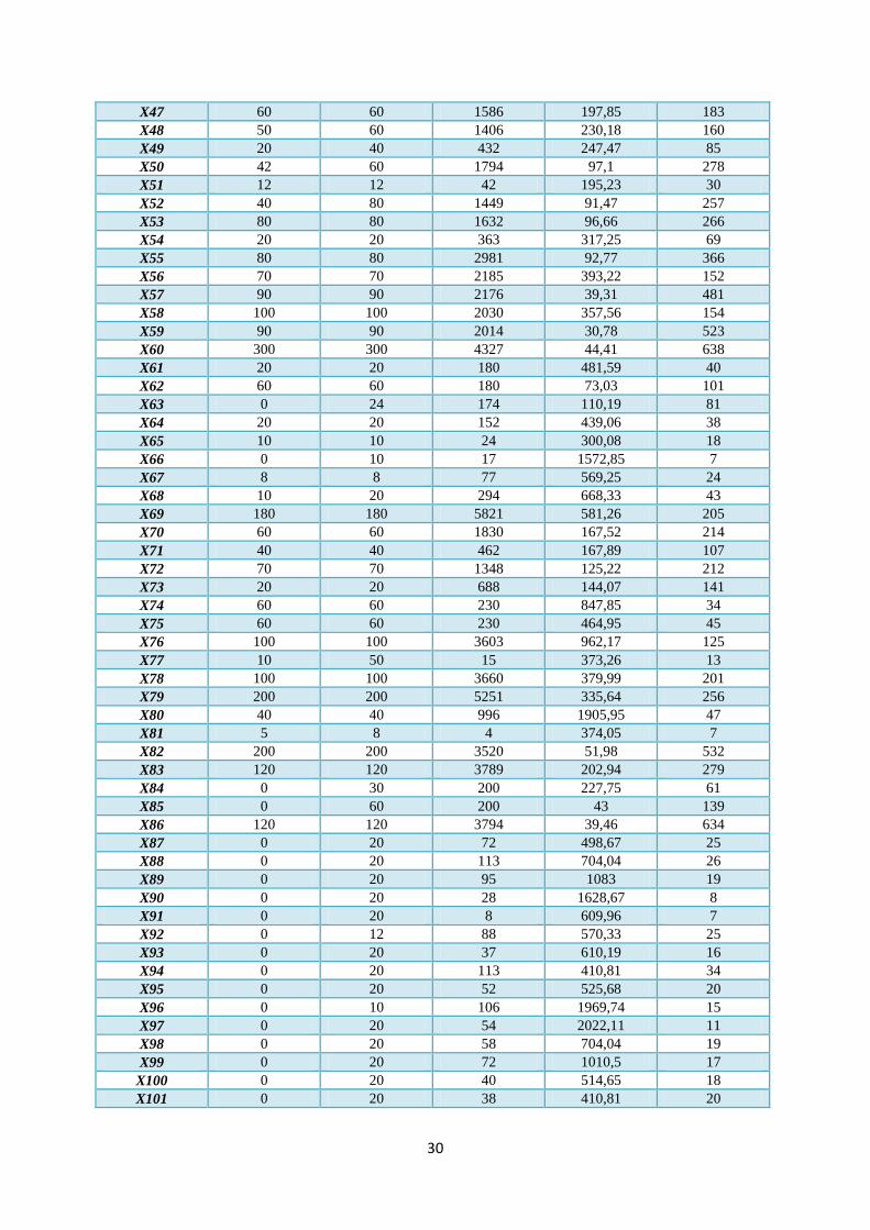
30

X47 60 60 1586 197,85 183

X48 50 60 1406 230,18 160

X49 20 40 432 247,47 85

X50 42 60 1794 97,1 278

X51 12 12 42 195,23 30

X52 40 80 1449 91,47 257

X53 80 80 1632 96,66 266

X54 20 20 363 317,25 69

X55 80 80 2981 92,77 366

X56 70 70 2185 393,22 152

X57 90 90 2176 39,31 481

X58 100 100 2030 357,56 154

X59 90 90 2014 30,78 523

X60 300 300 4327 44,41 638

X61 20 20 180 481,59 40

X62 60 60 180 73,03 101

X63 0 24 174 110,19 81

X64 20 20 152 439,06 38

X65 10 10 24 300,08 18

X66 0 10 17 1572,85 7

X67 8 8 77 569,25 24

X68 10 20 294 668,33 43

X69 180 180 5821 581,26 205

X70 60 60 1830 167,52 214

X71 40 40 462 167,89 107

X72 70 70 1348 125,22 212

X73 20 20 688 144,07 141

X74 60 60 230 847,85 34

X75 60 60 230 464,95 45

X76 100 100 3603 962,17 125

X77 10 50 15 373,26 13

X78 100 100 3660 379,99 201

X79 200 200 5251 335,64 256

X80 40 40 996 1905,95 47

X81 5 8 4 374,05 7

X82 200 200 3520 51,98 532

X83 120 120 3789 202,94 279

X84 0 30 200 227,75 61

X85 0 60 200 43 139

X86 120 120 3794 39,46 634

X87 0 20 72 498,67 25

X88 0 20 113 704,04 26

X89 0 20 95 1083 19

X90 0 20 28 1628,67 8

X91 0 20 8 609,96 7

X92 0 12 88 570,33 25

X93 0 20 37 610,19 16

X94 0 20 113 410,81 34

X95 0 20 52 525,68 20

X96 0 10 106 1969,74 15

X97 0 20 54 2022,11 11

X98 0 20 58 704,04 19

X99 0 20 72 1010,5 17

X100 0 20 40 514,65 18

X101 0 20 38 410,81 20

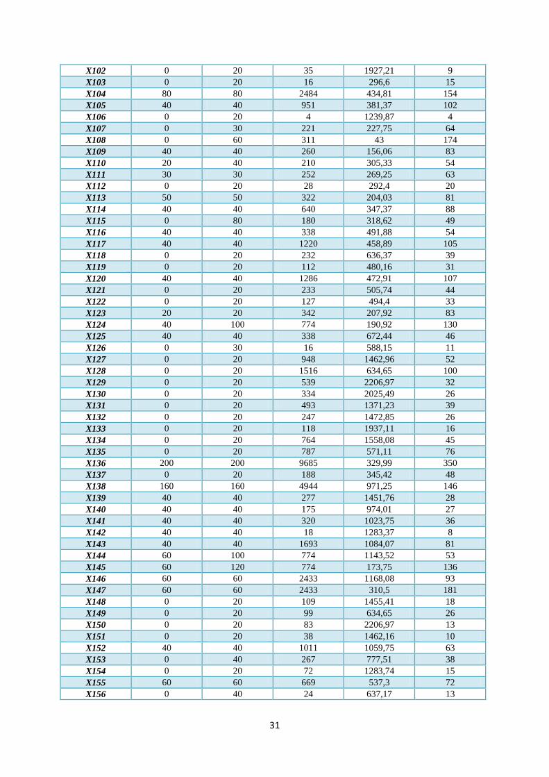
31

X102 0 20 35 1927,21 9

X103 0 20 16 296,6 15

X104 80 80 2484 434,81 154

X105 40 40 951 381,37 102

X106 0 20 4 1239,87 4

X107 0 30 221 227,75 64

X108 0 60 311 43 174

X109 40 40 260 156,06 83

X110 20 40 210 305,33 54

X111 30 30 252 269,25 63

X112 0 20 28 292,4 20

X113 50 50 322 204,03 81

X114 40 40 640 347,37 88

X115 0 80 180 318,62 49

X116 40 40 338 491,88 54

X117 40 40 1220 458,89 105

X118 0 20 232 636,37 39

X119 0 20 112 480,16 31

X120 40 40 1286 472,91 107

X121 0 20 233 505,74 44

X122 0 20 127 494,4 33

X123 20 20 342 207,92 83

X124 40 100 774 190,92 130

X125 40 40 338 672,44 46

X126 0 30 16 588,15 11

X127 0 20 948 1462,96 52

X128 0 20 1516 634,65 100

X129 0 20 539 2206,97 32

X130 0 20 334 2025,49 26

X131 0 20 493 1371,23 39

X132 0 20 247 1472,85 26

X133 0 20 118 1937,11 16

X134 0 20 764 1558,08 45

X135 0 20 787 571,11 76

X136 200 200 9685 329,99 350

X137 0 20 188 345,42 48

X138 160 160 4944 971,25 146

X139 40 40 277 1451,76 28

X140 40 40 175 974,01 27

X141 40 40 320 1023,75 36

X142 40 40 18 1283,37 8

X143 40 40 1693 1084,07 81

X144 60 100 774 1143,52 53

X145 60 120 774 173,75 136

X146 60 60 2433 1168,08 93

X147 60 60 2433 310,5 181

X148 0 20 109 1455,41 18

X149 0 20 99 634,65 26

X150 0 20 83 2206,97 13

X151 0 20 38 1462,16 10

X152 40 40 1011 1059,75 63

X153 0 40 267 777,51 38

X154 0 20 72 1283,74 15

X155 60 60 669 537,3 72

X156 0 40 24 637,17 13

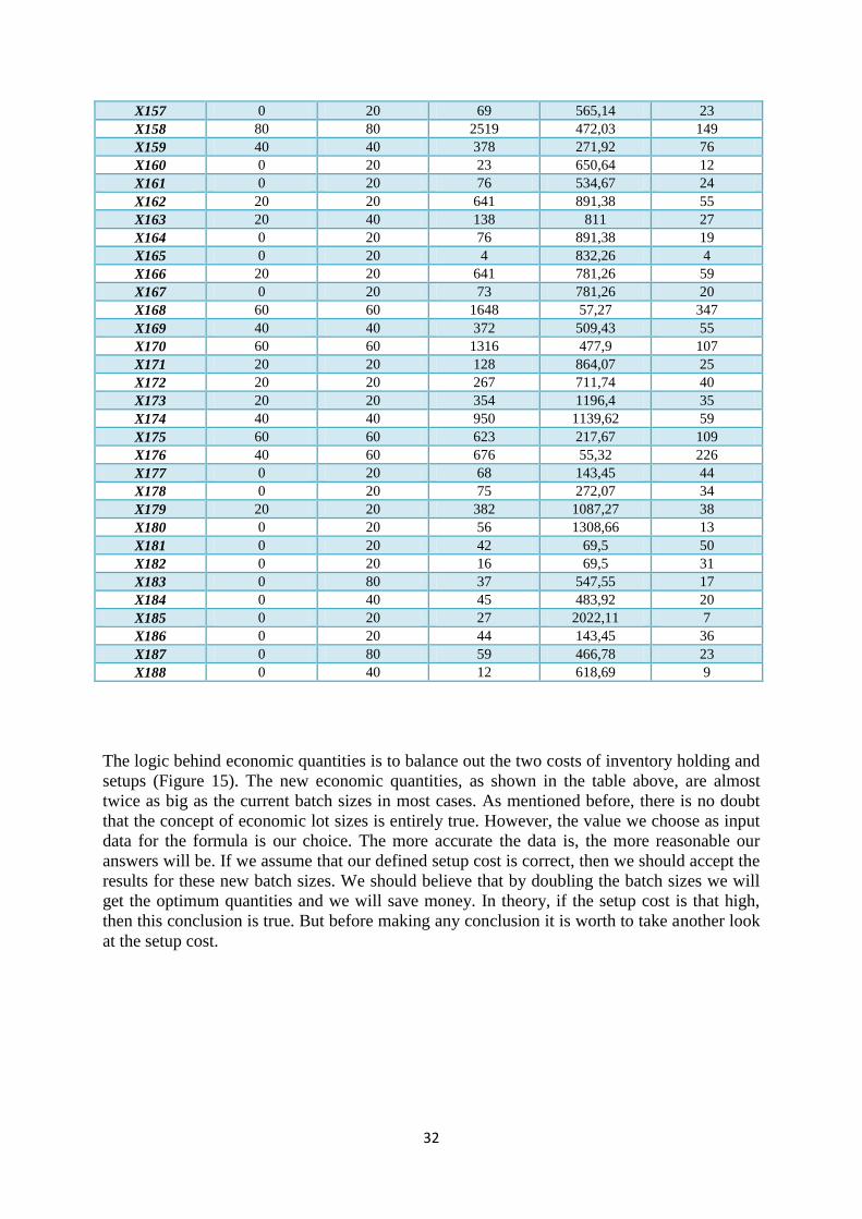
32

X157 0 20 69 565,14 23

X158 80 80 2519 472,03 149

X159 40 40 378 271,92 76

X160 0 20 23 650,64 12

X161 0 20 76 534,67 24

X162 20 20 641 891,38 55

X163 20 40 138 811 27

X164 0 20 76 891,38 19

X165 0 20 4 832,26 4

X166 20 20 641 781,26 59

X167 0 20 73 781,26 20

X168 60 60 1648 57,27 347

X169 40 40 372 509,43 55

X170 60 60 1316 477,9 107

X171 20 20 128 864,07 25

X172 20 20 267 711,74 40

X173 20 20 354 1196,4 35

X174 40 40 950 1139,62 59

X175 60 60 623 217,67 109

X176 40 60 676 55,32 226

X177 0 20 68 143,45 44

X178 0 20 75 272,07 34

X179 20 20 382 1087,27 38

X180 0 20 56 1308,66 13

X181 0 20 42 69,5 50

X182 0 20 16 69,5 31

X183 0 80 37 547,55 17

X184 0 40 45 483,92 20

X185 0 20 27 2022,11 7

X186 0 20 44 143,45 36

X187 0 80 59 466,78 23

X188 0 40 12 618,69 9

The logic behind economic quantities is to balance out the two costs of inventory holding and

setups (Figure 15). The new economic quantities, as shown in the table above, are almost

twice as big as the current batch sizes in most cases. As mentioned before, there is no doubt

that the concept of economic lot sizes is entirely true. However, the value we choose as input

data for the formula is our choice. The more accurate the data is, the more reasonable our

answers will be. If we assume that our defined setup cost is correct, then we should accept the

results for these new batch sizes. We should believe that by doubling the batch sizes we will

get the optimum quantities and we will save money. In theory, if the setup cost is that high,

then this conclusion is true. But before making any conclusion it is worth to take another look

at the setup cost.

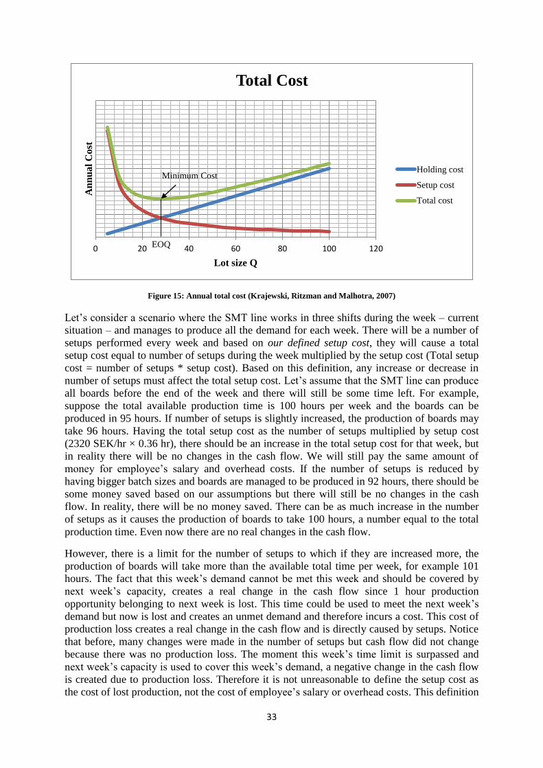
33

Figure 15: Annual total cost (Krajewski, Ritzman and Malhotra, 2007)

Let’s consider a scenario where the SMT line works in three shifts during the week – current

situation – and manages to produce all the demand for each week. There will be a number of

setups performed every week and based on our defined setup cost, they will cause a total

setup cost equal to number of setups during the week multiplied by the setup cost (Total setup

cost = number of setups * setup cost). Based on this definition, any increase or decrease in

number of setups must affect the total setup cost. Let’s assume that the SMT line can produce

all boards before the end of the week and there will still be some time left. For example,

suppose the total available production time is 100 hours per week and the boards can be

produced in 95 hours. If number of setups is slightly increased, the production of boards may

take 96 hours. Having the total setup cost as the number of setups multiplied by setup cost

(2320 SEK/hr × 0.36 hr), there should be an increase in the total setup cost for that week, but

in reality there will be no changes in the cash flow. We will still pay the same amount of

money for employee’s salary and overhead costs. If the number of setups is reduced by

having bigger batch sizes and boards are managed to be produced in 92 hours, there should be

some money saved based on our assumptions but there will still be no changes in the cash

flow. In reality, there will be no money saved. There can be as much increase in the number

of setups as it causes the production of boards to take 100 hours, a number equal to the total

production time. Even now there are no real changes in the cash flow.

However, there is a limit for the number of setups to which if they are increased more, the

production of boards will take more than the available total time per week, for example 101

hours. The fact that this week’s demand cannot be met this week and should be covered by

next week’s capacity, creates a real change in the cash flow since 1 hour production

opportunity belonging to next week is lost. This time could be used to meet the next week’s

demand but now is lost and creates an unmet demand and therefore incurs a cost. This cost of

production loss creates a real change in the cash flow and is directly caused by setups. Notice

that before, many changes were made in the number of setups but cash flow did not change

because there was no production loss. The moment this week’s time limit is surpassed and

next week’s capacity is used to cover this week’s demand, a negative change in the cash flow

is created due to production loss. Therefore it is not unreasonable to define the setup cost as

the cost of lost production, not the cost of employee’s salary or overhead costs. This definition

0 20 40 60 80 100 120

An

nu

al

Co

st

Lot size Q

Total Cost

Holding cost

Setup cost

Total cost

Minimum Cost

EOQ

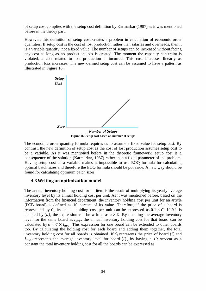
34

of setup cost complies with the setup cost definition by Karmarkar (1987) as it was mentioned

before in the theory part.

However, this definition of setup cost creates a problem in calculation of economic order

quantities. If setup cost is the cost of lost production rather than salaries and overheads, then it

is a variable quantity, not a fixed value. The number of setups can be increased without facing

any cost as long as no production loss is created. The moment the capacity constraint is

violated, a cost related to lost production is incurred. This cost increases linearly as

production loss increases. The new defined setup cost can be assumed to have a pattern as

illustrated in Figure 16:

Figure 16: Setup cost based on number of setups

The economic order quantity formula requires us to assume a fixed value for setup cost. By

contrast, the new definition of setup cost as the cost of lost production assumes setup cost to

be a variable. As it was mentioned before in the theoretic framework, setup cost is a

consequence of the solution (Karmarkar, 1987) rather than a fixed parameter of the problem.

Having setup cost as a variable makes it impossible to use EOQ formula for calculating

optimal batch sizes and therefore the EOQ formula should be put aside. A new way should be

found for calculating optimum batch sizes.

4.3 Writing an optimization model

The annual inventory holding cost for an item is the result of multiplying its yearly average

inventory level by its annual holding cost per unit. As it was mentioned before, based on the

information from the financial department, the inventory holding cost per unit for an article

(PCB board) is defined as 10 percent of its value. Therefore, if the price of a board is

represented by , its annual holding cost per unit can be expressed as . If 0.1 is

denoted by ( ), the expression can be written as . By denoting the average inventory

level for the same board as , the annual inventory holding cost for that board can be

calculated by . This expression for one board can be extended to other boards

too. By calculating the holding cost for each board and adding them together, the total

inventory holding cost for all boards is obtained. If represents the price of board ( ) and

represents the average inventory level for board ( ) , by having a 10 percent as a

constant the total inventory holding cost for all the boards can be expressed as:

Setup

Cost

Number of Setups

Zero

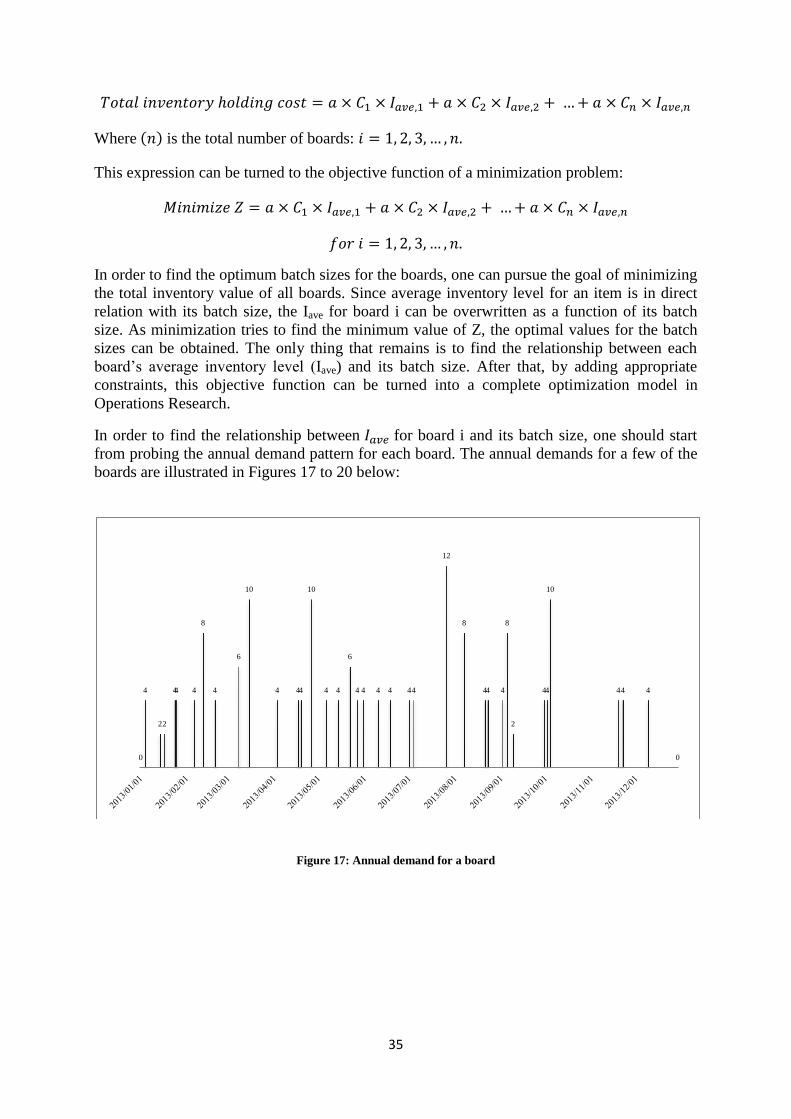
35

Where ( ) is the total number of boards:

This expression can be turned to the objective function of a minimization problem:

In order to find the optimum batch sizes for the boards, one can pursue the goal of minimizing

the total inventory value of all boards. Since average inventory level for an item is in direct

relation with its batch size, the Iave for board i can be overwritten as a function of its batch

size. As minimization tries to find the minimum value of Z, the optimal values for the batch

sizes can be obtained. The only thing that remains is to find the relationship between each

board’s average inventory level (Iave) and its batch size. After that, by adding appropriate

constraints, this objective function can be turned into a complete optimization model in

Operations Research.

In order to find the relationship between for board i and its batch size, one should start

from probing the annual demand pattern for each board. The annual demands for a few of the

boards are illustrated in Figures 17 to 20 below:

Figure 17: Annual demand for a board

0

4

2 2

4 4 4

8

4

6

10

4 4 4

10

4 4

6

4 4 4 4 4 4

12

8

4 4 4

8

2

4 4

10

4 4 4

0

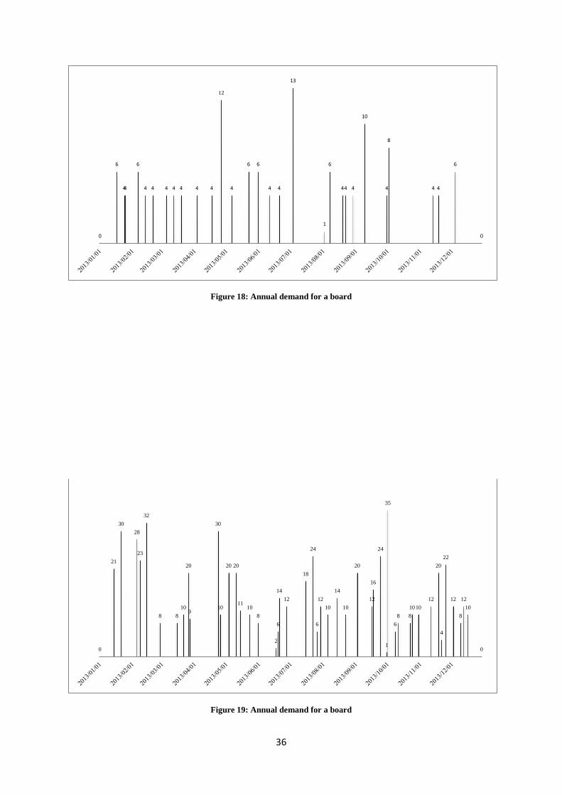
36

Figure 18: Annual demand for a board

Figure 19: Annual demand for a board

0

6

4 4

6

4 4 4 4 4 4 4

12

4

6 6

4 4

13

1

6

4 4 4

10

4

8

4 4

6

0

0

21

30

28

23

32

8 8

10

20

9

30

10

20 20

11 10

8

2

6

14

12

18

24

6

12

10

14

10

20

12

16

24

1

35

6

8 8

10 10

12

20

4

22

12

8

12

10

0

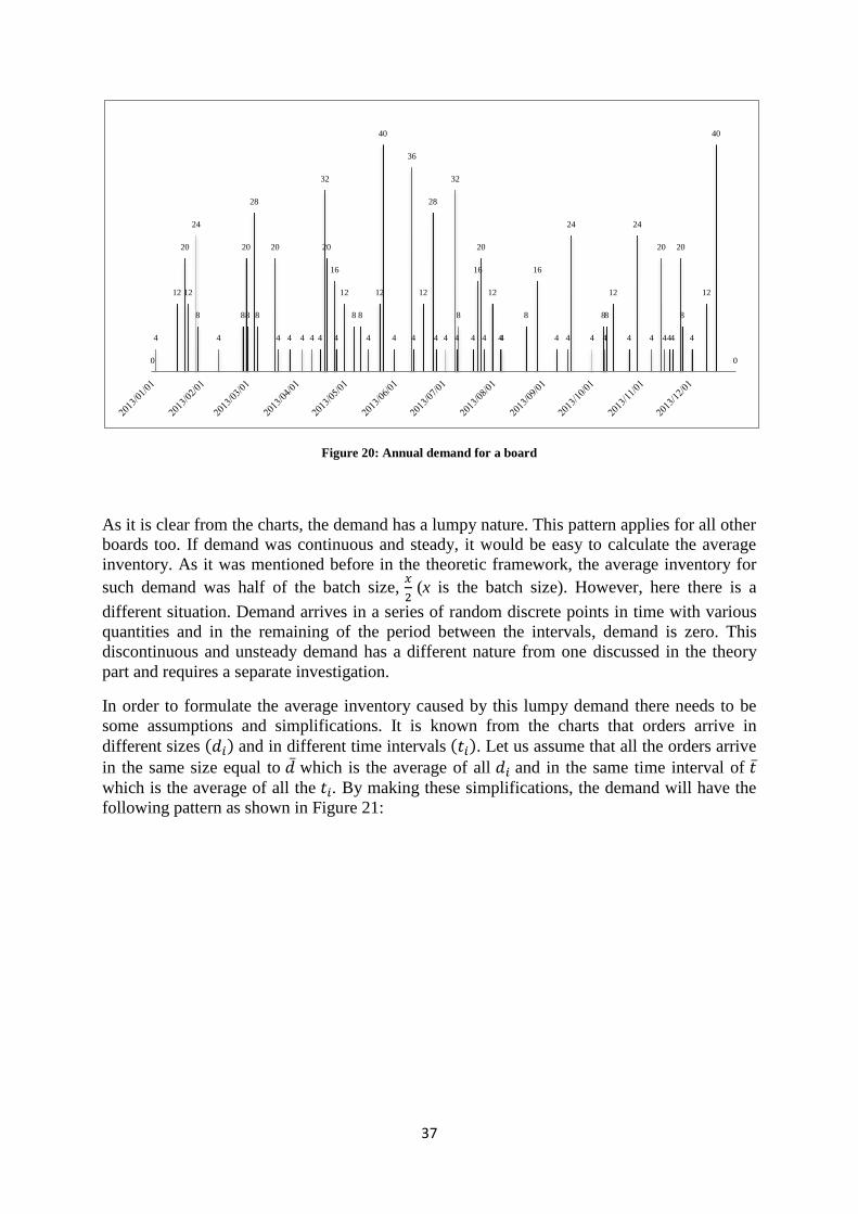
37

Figure 20: Annual demand for a board

As it is clear from the charts, the demand has a lumpy nature. This pattern applies for all other

boards too. If demand was continuous and steady, it would be easy to calculate the average

inventory. As it was mentioned before in the theoretic framework, the average inventory for

such demand was half of the batch size,

(x is the batch size). However, here there is a

different situation. Demand arrives in a series of random discrete points in time with various

quantities and in the remaining of the period between the intervals, demand is zero. This

discontinuous and unsteady demand has a different nature from one discussed in the theory

part and requires a separate investigation.

In order to formulate the average inventory caused by this lumpy demand there needs to be

some assumptions and simplifications. It is known from the charts that orders arrive in

different sizes ( ) and in different time intervals ( ). Let us assume that all the orders arrive

in the same size equal to which is the average of all and in the same time interval of which is the average of all the . By making these simplifications, the demand will have the

following pattern as shown in Figure 21:

0

4

12

20

12

24

8

4

8

20

8

28

8

20

4 4 4 4 4

32

20

16

4

12

8 8

4

12

40

4

36

4

12

28

4 4

32

4

8

4

16

20

4

12

4 4

8

16

4 4

24

4

8

4

8

12

4

24

4

20

4 4 4

20

8

4

12

40

0

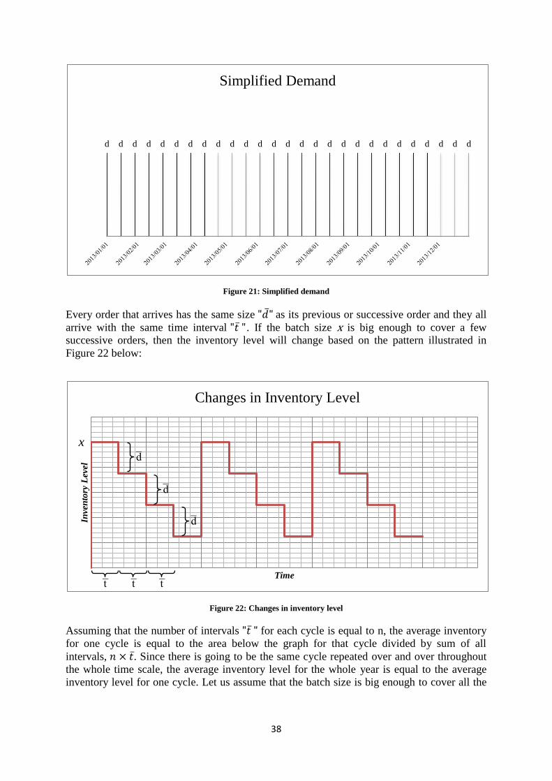
38

Figure 21: Simplified demand

Every order that arrives has the same size as its previous or successive order and they all

arrive with the same time interval . If the batch size x is big enough to cover a few

successive orders, then the inventory level will change based on the pattern illustrated in

Figure 22 below:

Figure 22: Changes in inventory level

Assuming that the number of intervals for each cycle is equal to n, the average inventory

for one cycle is equal to the area below the graph for that cycle divided by sum of all

intervals, . Since there is going to be the same cycle repeated over and over throughout

the whole time scale, the average inventory level for the whole year is equal to the average

inventory level for one cycle. Let us assume that the batch size is big enough to cover all the

d d d d d d d d d d d d d d d d d d d d d d d d d d d

Simplified Demand In

ven

tory

Lev

el

Time

Changes in Inventory Level

x d

d

d

t t t

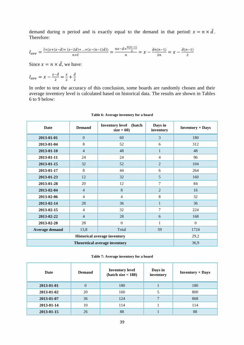
39

demand during n period and is exactly equal to the demand in that period: .

Therefore:

( ( ) ( ) ( ( ) ))

( )

( )

( )

Since , we have:

In order to test the accuracy of this conclusion, some boards are randomly chosen and their

average inventory level is calculated based on historical data. The results are shown in Tables

6 to 9 below:

Table 6: Average inventory for a board

Date Demand Inventory level (batch

size = 60)

Days in

inventory Inventory × Days

2013-01-01 0 60 3 180

2013-01-04 8 52 6 312

2013-01-10 4 48 1 48

2013-01-11 24 24 4 96

2013-01-15 32 52 2 104

2013-01-17 8 44 6 264

2013-01-23 12 32 5 160

2013-01-28 20 12 7 84

2013-02-04 4 8 2 16

2013-02-06 4 4 8 32

2013-02-14 28 36 1 36

2013-02-15 4 32 7 224

2013-02-22 4 28 6 168

2013-02-28 28 0 1 0

Average demand 13,8 Total 59 1724

Historical average inventory 29,2

Theoretical average inventory 36,9

Table 7: Average inventory for a board

Date Demand Inventory level

(batch size = 180)

Days in

inventory Inventory × Days

2013-01-01 0 180 1 180

2013-01-02 20 160 5 800

2013-01-07 36 124 7 868

2013-01-14 10 114 1 114

2013-01-15 26 88 1 88

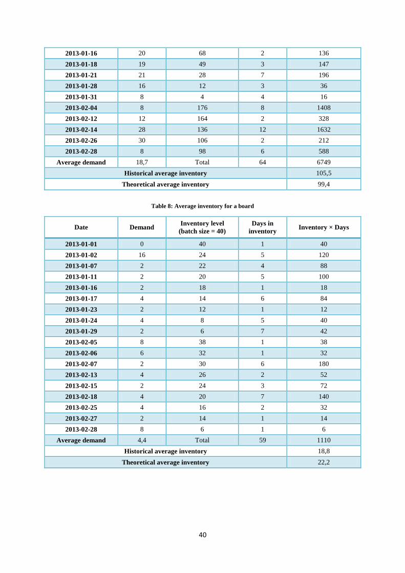
40

2013-01-16 20 68 2 136

2013-01-18 19 49 3 147

2013-01-21 21 28 7 196

2013-01-28 16 12 3 36

2013-01-31 8 4 4 16

2013-02-04 8 176 8 1408

2013-02-12 12 164 2 328

2013-02-14 28 136 12 1632

2013-02-26 30 106 2 212

2013-02-28 8 98 6 588

Average demand 18,7 Total 64 6749

Historical average inventory 105,5

Theoretical average inventory 99,4

Table 8: Average inventory for a board

Date Demand Inventory level

(batch size = 40)

Days in

inventory Inventory × Days

2013-01-01 0 40 1 40

2013-01-02 16 24 5 120

2013-01-07 2 22 4 88

2013-01-11 2 20 5 100

2013-01-16 2 18 1 18

2013-01-17 4 14 6 84

2013-01-23 2 12 1 12

2013-01-24 4 8 5 40

2013-01-29 2 6 7 42

2013-02-05 8 38 1 38

2013-02-06 6 32 1 32

2013-02-07 2 30 6 180

2013-02-13 4 26 2 52

2013-02-15 2 24 3 72

2013-02-18 4 20 7 140

2013-02-25 4 16 2 32

2013-02-27 2 14 1 14

2013-02-28 8 6 1 6

Average demand 4,4 Total 59 1110

Historical average inventory 18,8

Theoretical average inventory 22,2

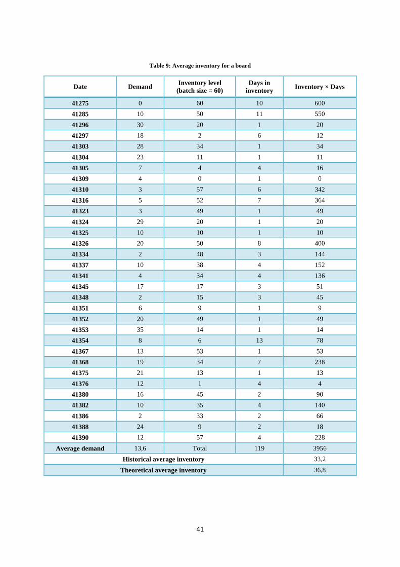
41

Table 9: Average inventory for a board

Date Demand Inventory level

(batch size = 60)

Days in

inventory Inventory × Days

41275 0 60 10 600

41285 10 50 11 550

41296 30 20 1 20

41297 18 2 6 12

41303 28 34 1 34

41304 23 11 1 11

41305 7 4 4 16

41309 4 0 1 0

41310 3 57 6 342

41316 5 52 7 364

41323 3 49 1 49

41324 29 20 1 20

41325 10 10 1 10

41326 20 50 8 400

41334 2 48 3 144

41337 10 38 4 152

41341 4 34 4 136

41345 17 17 3 51

41348 2 15 3 45

41351 6 9 1 9

41352 20 49 1 49

41353 35 14 1 14

41354 8 6 13 78

41367 13 53 1 53

41368 19 34 7 238

41375 21 13 1 13

41376 12 1 4 4

41380 16 45 2 90

41382 10 35 4 140

41386 2 33 2 66

41388 24 9 2 18

41390 12 57 4 228

Average demand 13,6 Total 119 3956

Historical average inventory 33,2

Theoretical average inventory 36,8

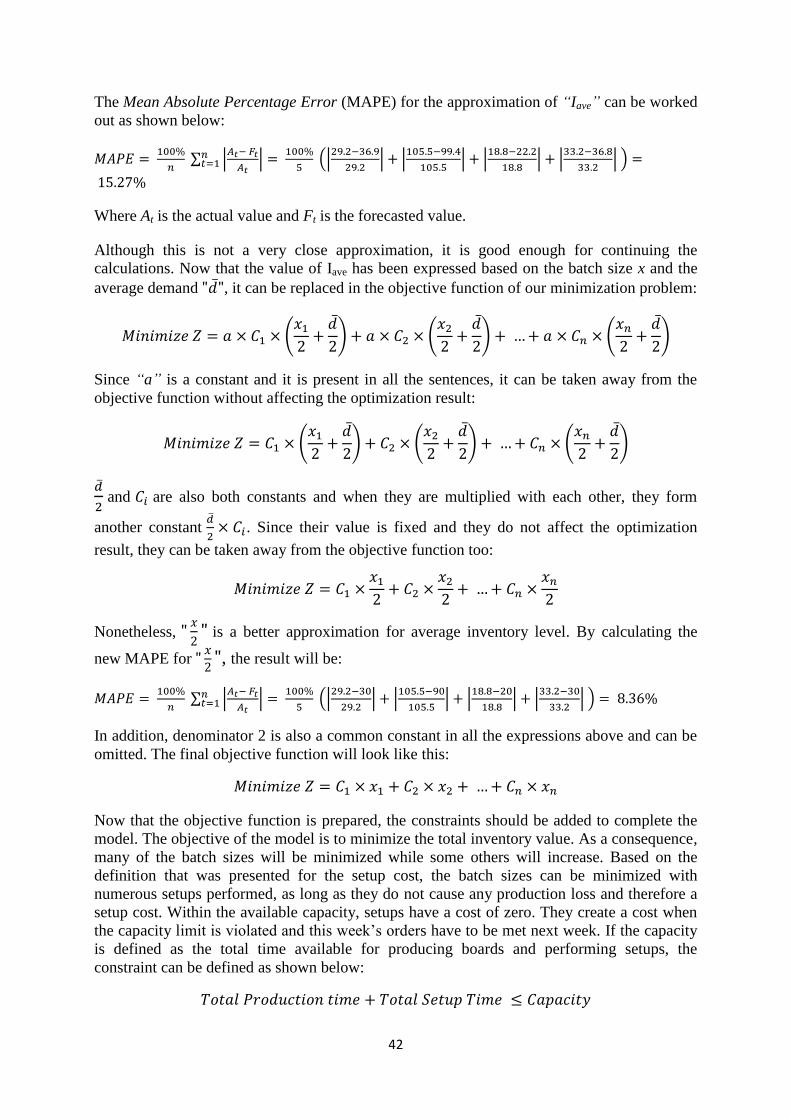
42

The Mean Absolute Percentage Error (MAPE) for the approximation of “Iave” can be worked

out as shown below:

∑ |

|

(|

| |

| |

| |

| )

Where At is the actual value and Ft is the forecasted value.

Although this is not a very close approximation, it is good enough for continuing the

calculations. Now that the value of Iave has been expressed based on the batch size x and the

average demand , it can be replaced in the objective function of our minimization problem:

(

) (

) (

)

Since “a” is a constant and it is present in all the sentences, it can be taken away from the

objective function without affecting the optimization result:

(

) (

) (

)

and are also both constants and when they are multiplied with each other, they form

another constant

. Since their value is fixed and they do not affect the optimization

result, they can be taken away from the objective function too:

Nonetheless,

is a better approximation for average inventory level. By calculating the

new MAPE for

, the result will be:

∑ |

|

(|

| |

| |

| |

| )

In addition, denominator 2 is also a common constant in all the expressions above and can be

omitted. The final objective function will look like this:

Now that the objective function is prepared, the constraints should be added to complete the

model. The objective of the model is to minimize the total inventory value. As a consequence,

many of the batch sizes will be minimized while some others will increase. Based on the

definition that was presented for the setup cost, the batch sizes can be minimized with

numerous setups performed, as long as they do not cause any production loss and therefore a

setup cost. Within the available capacity, setups have a cost of zero. They create a cost when

the capacity limit is violated and this week’s orders have to be met next week. If the capacity

is defined as the total time available for producing boards and performing setups, the

constraint can be defined as shown below:

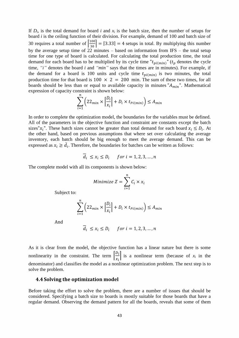
43

If Di, is the total demand for board i and xi is the batch size, then the number of setups for

board i is the ceiling function of their division. For example, demand of 100 and batch size of

30 requires a total number of ⌈

⌉ ⌈ ⌉ setups in total. By multiplying this number

by the average setup time of 22 minutes – based on information from IFS – the total setup

time for one type of board is calculated. For calculating the total production time, the total

demand for each board has to be multiplied by its cycle time ( ) ( denotes the cycle

time, “i” denotes the board i and “min” says that the times are in minutes). For example, if

the demand for a board is 100 units and cycle time ( ) is two minutes, the total

production time for that board is 100 × 2 = 200 min. The sum of these two times, for all

boards should be less than or equal to available capacity in minutes . Mathematical

expression of capacity constraint is shown below:

∑( ⌈ ⌉ ( ))

In order to complete the optimization model, the boundaries for the variables must be defined.

All of the parameters in the objective function and constraint are constants except the batch

sizes . These batch sizes cannot be greater than total demand for each board . At

the other hand, based on previous assumptions that where set over calculating the average

inventory, each batch should be big enough to meet the average demand. This can be

expressed as . Therefore, the boundaries for batches can be written as follows:

The complete model with all its components is shown below:

∑

Subject to:

∑( ⌈ ⌉ ( ))

And

As it is clear from the model, the objective function has a linear nature but there is some

nonlinearity in the constraint. The term ⌈

⌉ is a nonlinear term (because of xi in the

denominator) and classifies the model as a nonlinear optimization problem. The next step is to

solve the problem.

4.4 Solving the optimization model

Before taking the effort to solve the problem, there are a number of issues that should be

considered. Specifying a batch size to boards is mostly suitable for those boards that have a

regular demand. Observing the demand pattern for all the boards, reveals that some of them

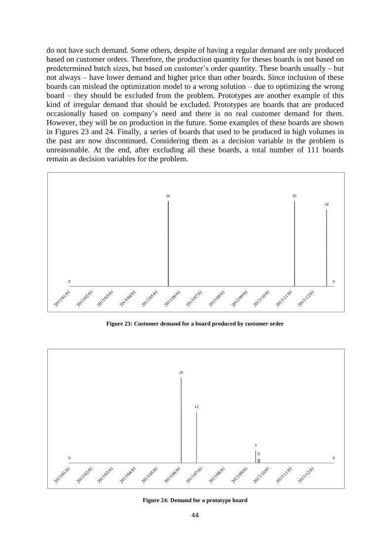
44

do not have such demand. Some others, despite of having a regular demand are only produced

based on customer orders. Therefore, the production quantity for theses boards is not based on

predetermined batch sizes, but based on customer’s order quantity. These boards usually – but

not always – have lower demand and higher price than other boards. Since inclusion of these

boards can mislead the optimization model to a wrong solution – due to optimizing the wrong

board – they should be excluded from the problem. Prototypes are another example of this

kind of irregular demand that should be excluded. Prototypes are boards that are produced

occasionally based on company’s need and there is no real customer demand for them.

However, they will be on production in the future. Some examples of these boards are shown

in Figures 23 and 24. Finally, a series of boards that used to be produced in high volumes in

the past are now discontinued. Considering them as a decision variable in the problem is

unreasonable. At the end, after excluding all these boards, a total number of 111 boards

remain as decision variables for the problem.

Figure 23: Customer demand for a board produced by customer order

Figure 24: Demand for a prototype board

0

20 20

18

0

0

20

12

3

1 1 0

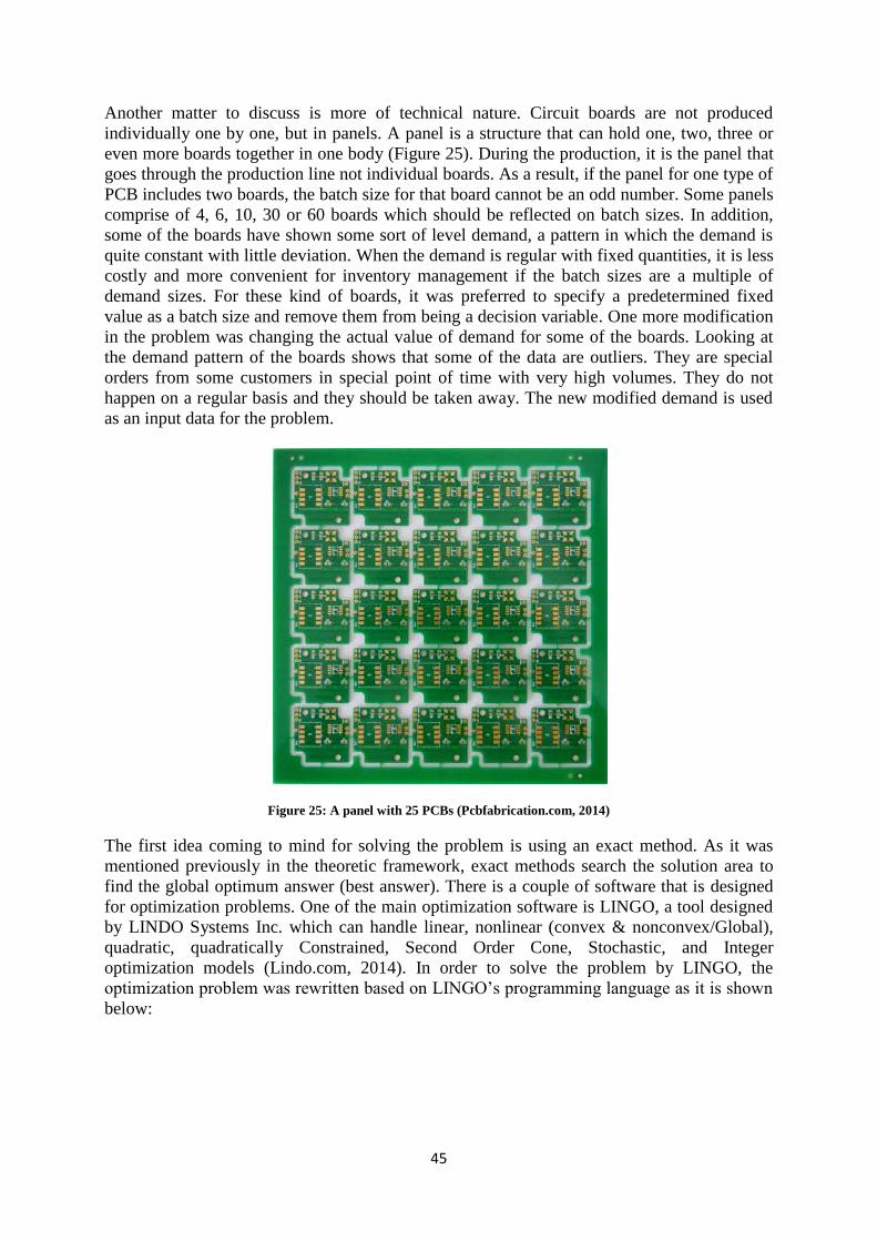
45

Another matter to discuss is more of technical nature. Circuit boards are not produced

individually one by one, but in panels. A panel is a structure that can hold one, two, three or

even more boards together in one body (Figure 25). During the production, it is the panel that

goes through the production line not individual boards. As a result, if the panel for one type of

PCB includes two boards, the batch size for that board cannot be an odd number. Some panels

comprise of 4, 6, 10, 30 or 60 boards which should be reflected on batch sizes. In addition,

some of the boards have shown some sort of level demand, a pattern in which the demand is

quite constant with little deviation. When the demand is regular with fixed quantities, it is less

costly and more convenient for inventory management if the batch sizes are a multiple of

demand sizes. For these kind of boards, it was preferred to specify a predetermined fixed

value as a batch size and remove them from being a decision variable. One more modification

in the problem was changing the actual value of demand for some of the boards. Looking at

the demand pattern of the boards shows that some of the data are outliers. They are special

orders from some customers in special point of time with very high volumes. They do not

happen on a regular basis and they should be taken away. The new modified demand is used

as an input data for the problem.

Figure 25: A panel with 25 PCBs (Pcbfabrication.com, 2014)

The first idea coming to mind for solving the problem is using an exact method. As it was

mentioned previously in the theoretic framework, exact methods search the solution area to

find the global optimum answer (best answer). There is a couple of software that is designed

for optimization problems. One of the main optimization software is LINGO, a tool designed

by LINDO Systems Inc. which can handle linear, nonlinear (convex & nonconvex/Global),

quadratic, quadratically Constrained, Second Order Cone, Stochastic, and Integer

optimization models (Lindo.com, 2014). In order to solve the problem by LINGO, the

optimization problem was rewritten based on LINGO’s programming language as it is shown

below:

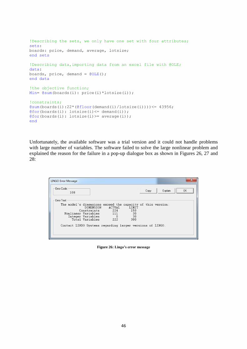
46

!Describing the sets, we only have one set with four attributes;

sets:

boards: price, demand, average, lotsize;

end sets

!Describing data,importing data from an excel file with @OLE;

data:

boards, price, demand = @OLE();

end data

!the objective function;

Min= @sum(boards(i): price(i)*lotsize(i));

!constraints;

@sum(boards(i):22*(@floor(demand(i)/lotsize(i))))<= 43956;

@for(boards(i): lotsize(i)<= demand(i));

@for(boards(i): lotsize(i)>= average(i));

end

Unfortunately, the available software was a trial version and it could not handle problems

with large number of variables. The software failed to solve the large nonlinear problem and

explained the reason for the failure in a pop-up dialogue box as shown in Figures 26, 27 and

28:

Figure 26: Lingo’s error message

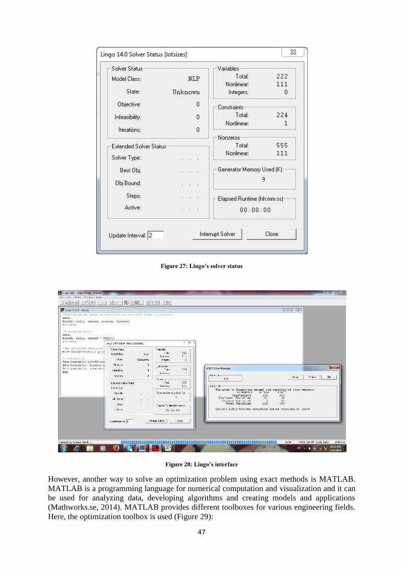
47

Figure 27: Lingo’s solver status

Figure 28: Lingo’s interface

However, another way to solve an optimization problem using exact methods is MATLAB.

MATLAB is a programming language for numerical computation and visualization and it can

be used for analyzing data, developing algorithms and creating models and applications

(Mathworks.se, 2014). MATLAB provides different toolboxes for various engineering fields.

Here, the optimization toolbox is used (Figure 29):

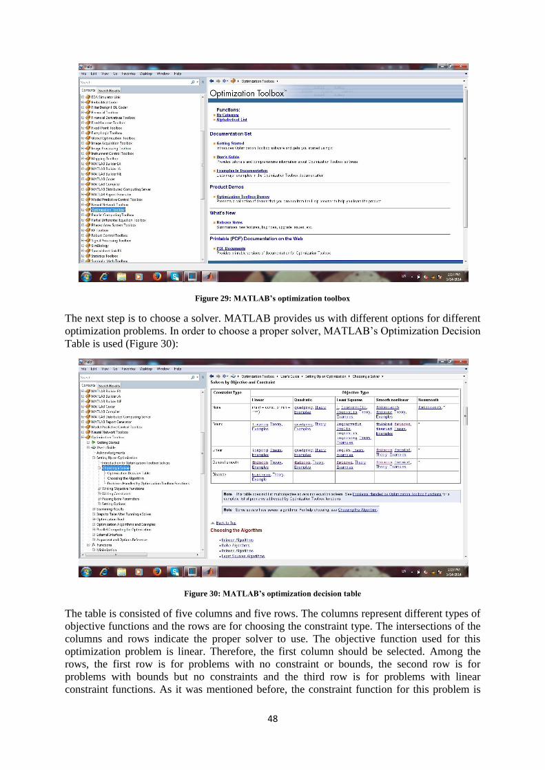
48

Figure 29: MATLAB’s optimization toolbox

The next step is to choose a solver. MATLAB provides us with different options for different

optimization problems. In order to choose a proper solver, MATLAB’s Optimization Decision

Table is used (Figure 30):

Figure 30: MATLAB’s optimization decision table

The table is consisted of five columns and five rows. The columns represent different types of

objective functions and the rows are for choosing the constraint type. The intersections of the

columns and rows indicate the proper solver to use. The objective function used for this

optimization problem is linear. Therefore, the first column should be selected. Among the

rows, the first row is for problems with no constraint or bounds, the second row is for

problems with bounds but no constraints and the third row is for problems with linear

constraint functions. As it was mentioned before, the constraint function for this problem is

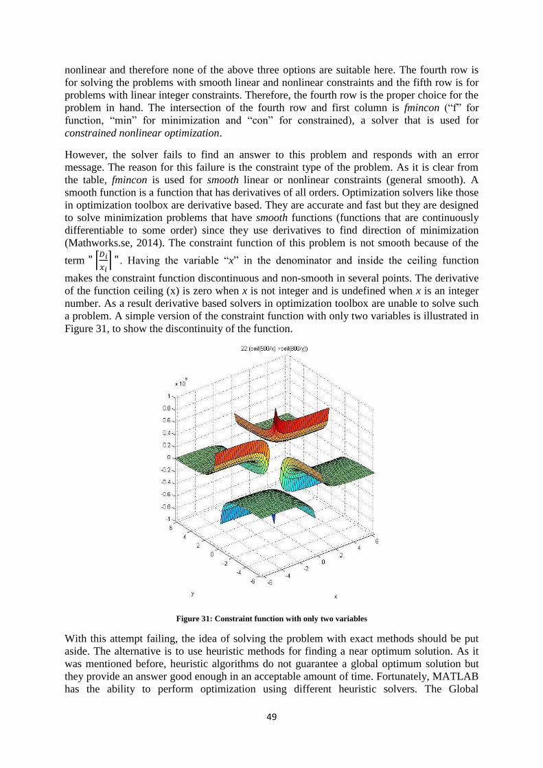
49

nonlinear and therefore none of the above three options are suitable here. The fourth row is

for solving the problems with smooth linear and nonlinear constraints and the fifth row is for

problems with linear integer constraints. Therefore, the fourth row is the proper choice for the

problem in hand. The intersection of the fourth row and first column is fmincon (“f” for

function, “min” for minimization and “con” for constrained), a solver that is used for

constrained nonlinear optimization.

However, the solver fails to find an answer to this problem and responds with an error

message. The reason for this failure is the constraint type of the problem. As it is clear from

the table, fmincon is used for smooth linear or nonlinear constraints (general smooth). A

smooth function is a function that has derivatives of all orders. Optimization solvers like those

in optimization toolbox are derivative based. They are accurate and fast but they are designed

to solve minimization problems that have smooth functions (functions that are continuously

differentiable to some order) since they use derivatives to find direction of minimization

(Mathworks.se, 2014). The constraint function of this problem is not smooth because of the

term ⌈

⌉ . Having the variable “x” in the denominator and inside the ceiling function

makes the constraint function discontinuous and non-smooth in several points. The derivative

of the function ceiling (x) is zero when x is not integer and is undefined when x is an integer

number. As a result derivative based solvers in optimization toolbox are unable to solve such

a problem. A simple version of the constraint function with only two variables is illustrated in

Figure 31, to show the discontinuity of the function.

Figure 31: Constraint function with only two variables

With this attempt failing, the idea of solving the problem with exact methods should be put

aside. The alternative is to use heuristic methods for finding a near optimum solution. As it

was mentioned before, heuristic algorithms do not guarantee a global optimum solution but

they provide an answer good enough in an acceptable amount of time. Fortunately, MATLAB

has the ability to perform optimization using different heuristic solvers. The Global

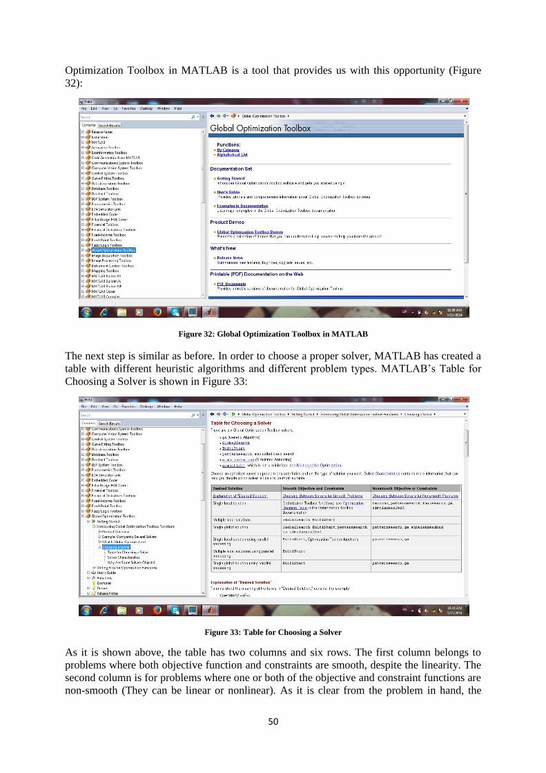
50

Optimization Toolbox in MATLAB is a tool that provides us with this opportunity (Figure

32):

Figure 32: Global Optimization Toolbox in MATLAB

The next step is similar as before. In order to choose a proper solver, MATLAB has created a

table with different heuristic algorithms and different problem types. MATLAB’s Table for

Choosing a Solver is shown in Figure 33:

Figure 33: Table for Choosing a Solver

As it is shown above, the table has two columns and six rows. The first column belongs to

problems where both objective function and constraints are smooth, despite the linearity. The

second column is for problems where one or both of the objective and constraint functions are

non-smooth (They can be linear or nonlinear). As it is clear from the problem in hand, the

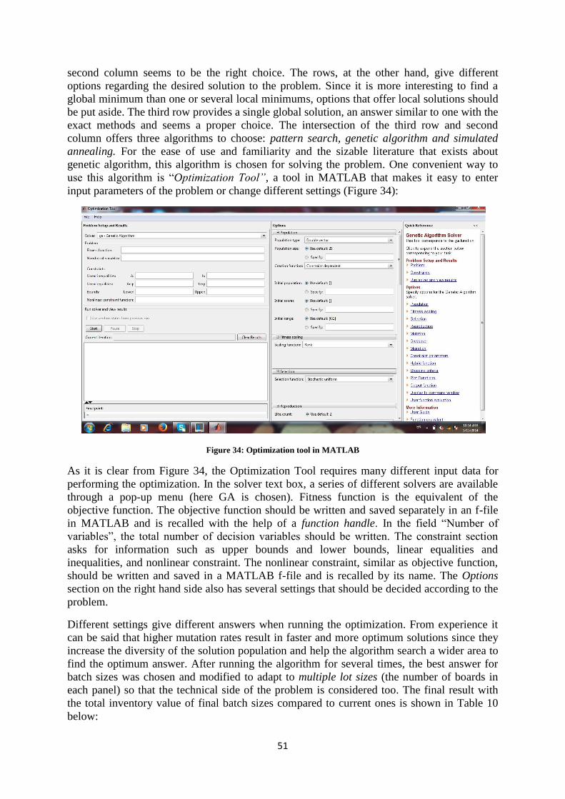
51

second column seems to be the right choice. The rows, at the other hand, give different

options regarding the desired solution to the problem. Since it is more interesting to find a

global minimum than one or several local minimums, options that offer local solutions should

be put aside. The third row provides a single global solution, an answer similar to one with the

exact methods and seems a proper choice. The intersection of the third row and second

column offers three algorithms to choose: pattern search, genetic algorithm and simulated

annealing. For the ease of use and familiarity and the sizable literature that exists about

genetic algorithm, this algorithm is chosen for solving the problem. One convenient way to

use this algorithm is “Optimization Tool”, a tool in MATLAB that makes it easy to enter

input parameters of the problem or change different settings (Figure 34):

Figure 34: Optimization tool in MATLAB

As it is clear from Figure 34, the Optimization Tool requires many different input data for

performing the optimization. In the solver text box, a series of different solvers are available

through a pop-up menu (here GA is chosen). Fitness function is the equivalent of the

objective function. The objective function should be written and saved separately in an f-file

in MATLAB and is recalled with the help of a function handle. In the field “Number of

variables”, the total number of decision variables should be written. The constraint section

asks for information such as upper bounds and lower bounds, linear equalities and

inequalities, and nonlinear constraint. The nonlinear constraint, similar as objective function,

should be written and saved in a MATLAB f-file and is recalled by its name. The Options

section on the right hand side also has several settings that should be decided according to the

problem.

Different settings give different answers when running the optimization. From experience it

can be said that higher mutation rates result in faster and more optimum solutions since they

increase the diversity of the solution population and help the algorithm search a wider area to

find the optimum answer. After running the algorithm for several times, the best answer for

batch sizes was chosen and modified to adapt to multiple lot sizes (the number of boards in

each panel) so that the technical side of the problem is considered too. The final result with

the total inventory value of final batch sizes compared to current ones is shown in Table 10

below:

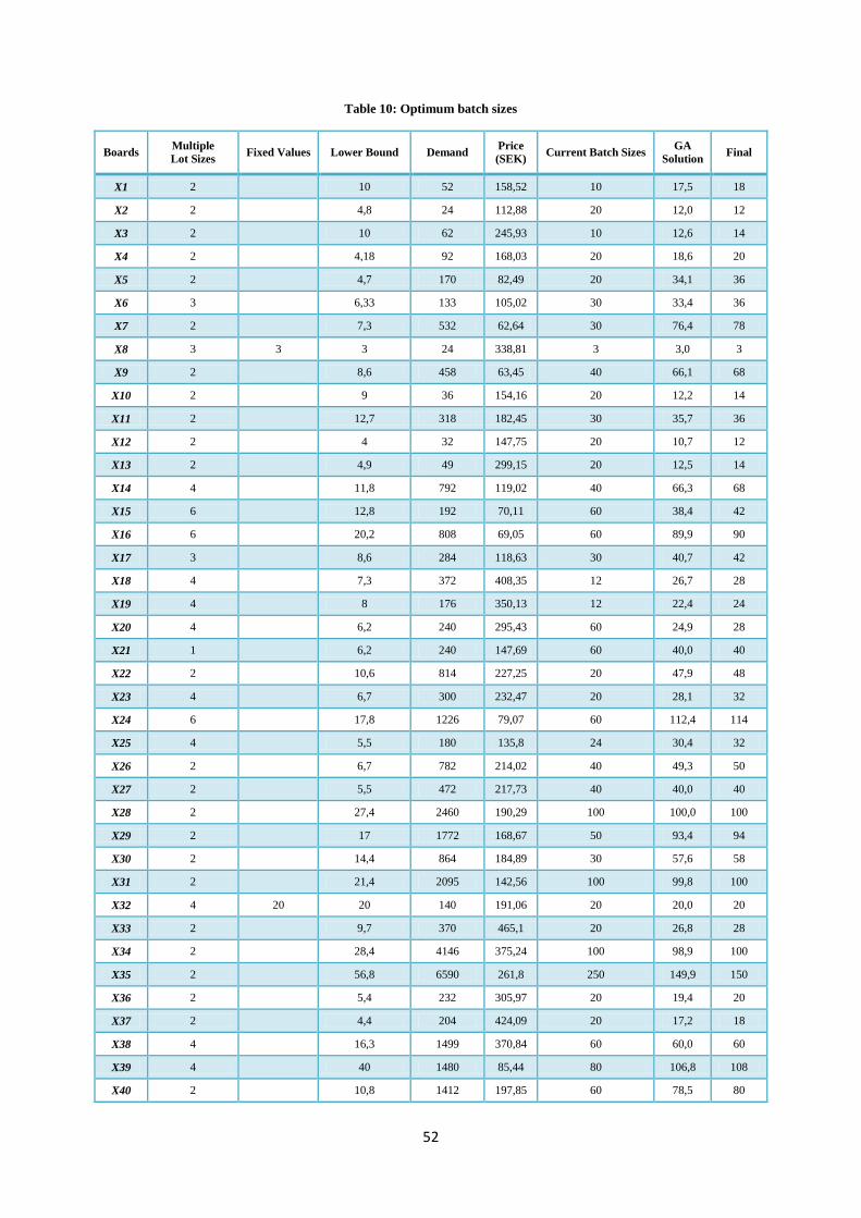
52

Table 10: Optimum batch sizes

Boards Multiple

Lot Sizes Fixed Values Lower Bound Demand

Price

(SEK) Current Batch Sizes

GA

Solution Final

X1 2

10 52 158,52 10 17,5 18

X2 2

4,8 24 112,88 20 12,0 12

X3 2

10 62 245,93 10 12,6 14

X4 2

4,18 92 168,03 20 18,6 20

X5 2

4,7 170 82,49 20 34,1 36

X6 3

6,33 133 105,02 30 33,4 36

X7 2

7,3 532 62,64 30 76,4 78

X8 3 3 3 24 338,81 3 3,0 3

X9 2

8,6 458 63,45 40 66,1 68

X10 2

9 36 154,16 20 12,2 14

X11 2

12,7 318 182,45 30 35,7 36

X12 2

4 32 147,75 20 10,7 12

X13 2

4,9 49 299,15 20 12,5 14

X14 4

11,8 792 119,02 40 66,3 68

X15 6

12,8 192 70,11 60 38,4 42

X16 6

20,2 808 69,05 60 89,9 90

X17 3

8,6 284 118,63 30 40,7 42

X18 4

7,3 372 408,35 12 26,7 28

X19 4

8 176 350,13 12 22,4 24

X20 4

6,2 240 295,43 60 24,9 28

X21 1

6,2 240 147,69 60 40,0 40

X22 2

10,6 814 227,25 20 47,9 48

X23 4

6,7 300 232,47 20 28,1 32

X24 6

17,8 1226 79,07 60 112,4 114

X25 4

5,5 180 135,8 24 30,4 32

X26 2

6,7 782 214,02 40 49,3 50

X27 2

5,5 472 217,73 40 40,0 40

X28 2

27,4 2460 190,29 100 100,0 100

X29 2

17 1772 168,67 50 93,4 94

X30 2

14,4 864 184,89 30 57,6 58

X31 2

21,4 2095 142,56 100 99,8 100

X32 4 20 20 140 191,06 20 20,0 20

X33 2

9,7 370 465,1 20 26,8 28

X34 2

28,4 4146 375,24 100 98,9 100

X35 2

56,8 6590 261,8 250 149,9 150

X36 2

5,4 232 305,97 20 19,4 20

X37 2

4,4 204 424,09 20 17,2 18

X38 4

16,3 1499 370,84 60 60,0 60

X39 4

40 1480 85,44 80 106,8 108

X40 2

10,8 1412 197,85 60 78,5 80

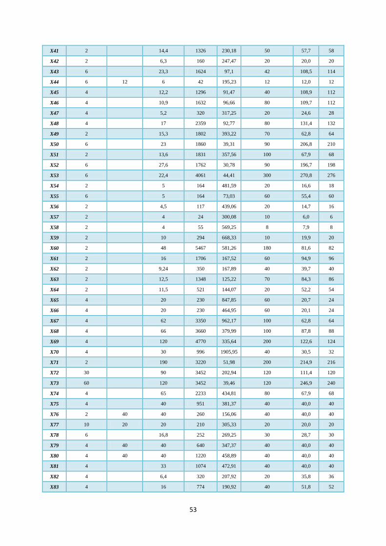
53

X41 2

14,4 1326 230,18 50 57,7 58

X42 2

6,3 160 247,47 20 20,0 20

X43 6

23,3 1624 97,1 42 108,5 114

X44 6 12 6 42 195,23 12 12,0 12

X45 4

12,2 1296 91,47 40 108,9 112

X46 4

10,9 1632 96,66 80 109,7 112

X47 4

5,2 320 317,25 20 24,6 28

X48 4

17 2359 92,77 80 131,4 132

X49 2

15,3 1802 393,22 70 62,8 64

X50 6

23 1860 39,31 90 206,8 210

X51 2

13,6 1831 357,56 100 67,9 68

X52 6

27,6 1762 30,78 90 196,7 198

X53 6

22,4 4061 44,41 300 270,8 276

X54 2

5 164 481,59 20 16,6 18

X55 6

5 164 73,03 60 55,4 60

X56 2

4,5 117 439,06 20 14,7 16

X57 2

4 24 300,08 10 6,0 6

X58 2

4 55 569,25 8 7,9 8

X59 2

10 294 668,33 10 19,9 20

X60 2

48 5467 581,26 180 81,6 82

X61 2

16 1706 167,52 60 94,9 96

X62 2

9,24 350 167,89 40 39,7 40

X63 2

12,5 1348 125,22 70 84,3 86

X64 2

11,5 521 144,07 20 52,2 54

X65 4

20 230 847,85 60 20,7 24

X66 4

20 230 464,95 60 20,1 24

X67 4

62 3350 962,17 100 62,8 64

X68 4

66 3660 379,99 100 87,8 88

X69 4

120 4770 335,64 200 122,6 124

X70 4

30 996 1905,95 40 30,5 32

X71 2

190 3220 51,98 200 214,9 216

X72 30

90 3452 202,94 120 111,4 120

X73 60

120 3452 39,46 120 246,9 240

X74 4

65 2233 434,81 80 67,9 68

X75 4

40 951 381,37 40 40,0 40

X76 2 40 40 260 156,06 40 40,0 40

X77 10 20 20 210 305,33 20 20,0 20

X78 6

16,8 252 269,25 30 28,7 30

X79 4 40 40 640 347,37 40 40,0 40

X80 4 40 40 1220 458,89 40 40,0 40

X81 4

33 1074 472,91 40 40,0 40

X82 4

6,4 320 207,92 20 35,8 36

X83 4

16 774 190,92 40 51,8 52

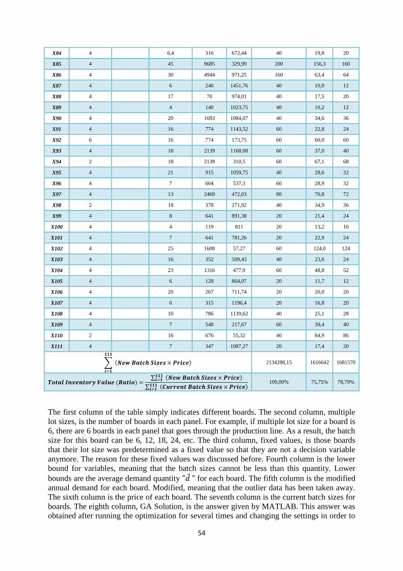
54

X84 4

6,4 316 672,44 40 19,8 20

X85 4

45 9685 329,99 200 156,3 160

X86 4

30 4944 971,25 160 63,4 64

X87 4

6 240 1451,76 40 10,0 12

X88 4

17 70 974,01 40 17,5 20

X89 4

4 140 1023,75 40 10,2 12

X90 4

20 1693 1084,07 40 34,6 36

X91 4

16 774 1143,52 60 22,8 24

X92 6

16 774 173,75 60 60,0 60

X93 4

18 2139 1168,08 60 37,0 40

X94 2

18 2139 310,5 60 67,1 68

X95 4

21 915 1059,75 40 28,6 32

X96 4

7 604 537,3 60 28,9 32

X97 4

13 2469 472,03 80 70,8 72

X98 2

18 378 271,92 40 34,9 36

X99 4

8 641 891,38 20 21,4 24

X100 4

4 119 811 20 13,2 16

X101 4

7 641 781,26 20 22,9 24

X102 4

25 1608 57,27 60 124,0 124

X103 4

16 352 509,43 40 23,6 24

X104 4

23 1316 477,9 60 48,8 52

X105 4

6 128 864,07 20 11,7 12

X106 4

20 267 711,74 20 20,0 20

X107 4

6 315 1196,4 20 16,8 20

X108 4

10 786 1139,62 40 25,1 28

X109 4

7 548 217,67 60 39,4 40

X110 2

16 676 55,32 40 84,9 86

X111 4

7 347 1087,27 20 17,4 20

∑ ( )

2134288,15 1616642 1681570

( ) ∑ ( )

∑ ( )

100,00% 75,75% 78,79%

The first column of the table simply indicates different boards. The second column, multiple

lot sizes, is the number of boards in each panel. For example, if multiple lot size for a board is

6, there are 6 boards in each panel that goes through the production line. As a result, the batch

size for this board can be 6, 12, 18, 24, etc. The third column, fixed values, is those boards

that their lot size was predetermined as a fixed value so that they are not a decision variable

anymore. The reason for these fixed values was discussed before. Fourth column is the lower

bound for variables, meaning that the batch sizes cannot be less than this quantity. Lower

bounds are the average demand quantity for each board. The fifth column is the modified

annual demand for each board. Modified, meaning that the outlier data has been taken away.

The sixth column is the price of each board. The seventh column is the current batch sizes for

boards. The eighth column, GA Solution, is the answer given by MATLAB. This answer was

obtained after running the optimization for several times and changing the settings in order to

55

improve the optimal solution. The reason that problem is not solved with integer values and

batch sizes are not complete integers is that it is much easier and faster for MATLAB to solve

problems with continuous values than integer ones. These values had to be modified to

comply with multiple lot sizes. The results are shown in column ninth, “Final”, as final

optimum batch sizes.

The last row in the table shows the ratio of total inventory value resulted from new batch sizes

over total inventory value resulted from current batch sizes. As it was mentioned before, the

average inventory level for a board is considered to be half the batch size. At worst, it can be

considered as a fraction of the batch size. However, when the total inventory values of new

and current batch sizes are divided over to calculate the ratio, these constants cancel out. The

formula used for calculating the ratio of total inventory value for two different batch sizes is

shown below:

∑ ( )

∑ ( )

∑ ( )

∑ ( )

As a result, the new batch sizes will reduce the total inventory value by 21.21% (100% -

78.79%).

4.5 Setup improvement

Setup times for the pick and place machines are quite long. To reduce the effect of long

setups, operators use the group setup strategy. In this strategy, boards with similar

components are grouped as one family and are produced sequentially. The software equipped

with the machines makes it possible to create different setup families from different boards.

Operators have access to the production plan for each day through IFS. Doing that, operators

know what boards have to be produced each day. They can choose some of the boards that

have similar components (based on their experience) and give their article numbers to the

software. The software, then, evaluates their compatibility considering their components and

the maximum number of positions available for feeders on the machine’s feeder bank. If they

can fit in to one family, software will produce a list of the required feeders and their exact

placement. The process of finding the optimum placement for feeders to increase the

production speed is done automatically by software and takes only a few seconds.

Since it is very likely that some of the components required for a new setup family is already

in use in the previous family (currently in the machine), one of the operators compares the

two different lists of components. Common components are found and their places on the

feeder banks are recorded and they will be used in the new setup family, in their new places.

The number of components in each list can differ based on the boards in the family but it is

very likely that at least one of the two feeder banks of the machine is completely full. Each

feeder bank (stage) has the capacity of 70 feeders. The process of finding the common feeders

used to be done manually, taking an average of five minutes but now it is an automatic

process.

In order to save time, those feeders that are not common between two sequential setups are

collected and put on a rack. Feeders are placed on the rack based on their orders in the list. If

one of the stages is already empty (it can happen if all the feeders in previous setup could fit

56

into one stage) it is not in operation and operators can put the feeders for the new setup on the

stage. This is called offline setup. However they can’t fill the places for common feeders and

they have to wait until the current operation is finished.

When the last board from the previous family leaves the machine, the machine can start its

setup process. Setup operations on each machine are performed by one, two or three

operators. However, there is no significant reduction in setup time when the number of

operators increases because the activities are not performed in parallel and there is no clear

division of labor or clear setup procedure that can exploit the increase in number of operators.

After the last scheduled panel of boards is produced, the two stages are distracted, meaning

that they move away from each other and make it possible for operators to change the feeders

or adjust and clean the nozzle. Then, there are a series of activities that are done:

The width of the conveyor belt that carries the panels is adjusted

The nozzle head is adjusted and cleaned if needed (this is done automatically)

An operator brings a wagon and picks up common feeders for the new setup (this is

done either by one operator looking at the list and picking up the feeders or by two

operators, one reading the list out loud and the other picking up the feeders)

The rest of the feeders that are not used in the new family setup are picked up and put

on the wagon

After emptying the two stages, common feeders are put on the stages in their specified

places; following them the new feeders are taken out from the rack and put on the

stages (this process also requires the list of components and their places. If it is done

by one person, he looks at the list and puts the feeders on the stage. If it is done by two

operators, one reads the list and the other puts the feeders on the stage)

The setup program is sent

The reels in the feeders are checked with a barcode scanner to check if they are at their

right location

The family setup time for pick and place machine of small components (CP) has an average

of 23 minutes with the standard deviation of 7 minutes while the total setup time for both

machines has an average of 35 minutes and a standard deviation of 2.

After making a number of observations of the setup process, a list of suggestions was

prepared that could help to reduce the setup time. The setup improvement process has four

conceptual stages. At stage zero or the preliminary stage, the internal and external setup

operations are not distinguished and what is done as internal setup can in fact be done

externally. In case of setup operations for pick and place machines, the process of putting the

feeders back on the shelves is an external setup while it is done as an internal setup. The

process takes 4 to 5 minutes in average. Another example of external setup performed

internally can be bringing of the wagon.

At stage 1, there is a clear distinction between internal and external setup operations. Those

operations that are external are performed before or after setup. A number of suggestions were

given to take away the external activities and reduce the setup time. For example putting the

feeders on the shelves can be done after the setup. One thing that was observed during the

setup was that when operators take out the feeders from the feeder banks (stages), they tend to

sort them in groups. That makes it easier for them to put them back on the shelves. This is

obviously an external operation that can be done after the setup. The four operations of taking

out the feeders, sorting them, putting them on the wagon and putting them back on the shelves

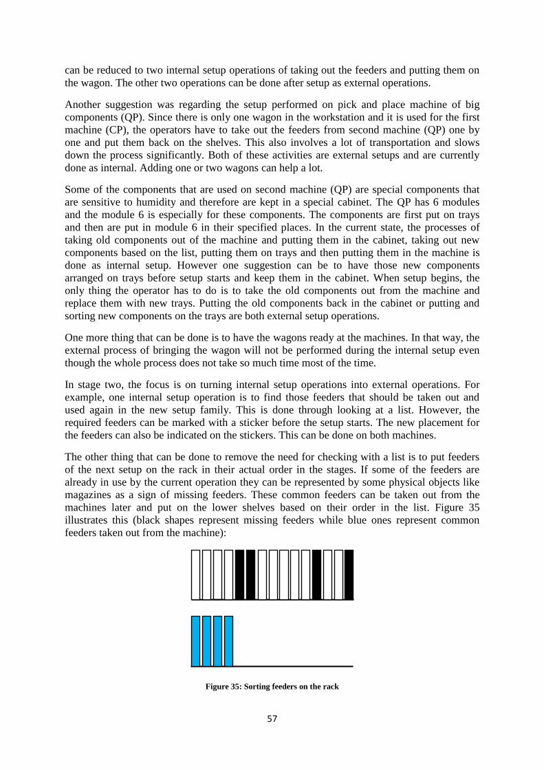
57

can be reduced to two internal setup operations of taking out the feeders and putting them on

the wagon. The other two operations can be done after setup as external operations.

Another suggestion was regarding the setup performed on pick and place machine of big

components (QP). Since there is only one wagon in the workstation and it is used for the first

machine (CP), the operators have to take out the feeders from second machine (QP) one by

one and put them back on the shelves. This also involves a lot of transportation and slows

down the process significantly. Both of these activities are external setups and are currently

done as internal. Adding one or two wagons can help a lot.

Some of the components that are used on second machine (QP) are special components that

are sensitive to humidity and therefore are kept in a special cabinet. The QP has 6 modules

and the module 6 is especially for these components. The components are first put on trays

and then are put in module 6 in their specified places. In the current state, the processes of

taking old components out of the machine and putting them in the cabinet, taking out new

components based on the list, putting them on trays and then putting them in the machine is

done as internal setup. However one suggestion can be to have those new components

arranged on trays before setup starts and keep them in the cabinet. When setup begins, the

only thing the operator has to do is to take the old components out from the machine and

replace them with new trays. Putting the old components back in the cabinet or putting and

sorting new components on the trays are both external setup operations.

One more thing that can be done is to have the wagons ready at the machines. In that way, the

external process of bringing the wagon will not be performed during the internal setup even

though the whole process does not take so much time most of the time.

In stage two, the focus is on turning internal setup operations into external operations. For

example, one internal setup operation is to find those feeders that should be taken out and

used again in the new setup family. This is done through looking at a list. However, the

required feeders can be marked with a sticker before the setup starts. The new placement for

the feeders can also be indicated on the stickers. This can be done on both machines.

The other thing that can be done to remove the need for checking with a list is to put feeders

of the next setup on the rack in their actual order in the stages. If some of the feeders are

already in use by the current operation they can be represented by some physical objects like

magazines as a sign of missing feeders. These common feeders can be taken out from the

machines later and put on the lower shelves based on their order in the list. Figure 35

illustrates this (black shapes represent missing feeders while blue ones represent common

feeders taken out from the machine):

Figure 35: Sorting feeders on the rack

58

Doing so, the operator can take the first four feeders (according to the picture) and put them

on the stages. Then he knows that there are two magazines or plastic parts that represent the

missing feeders. Therefore he takes two of the feeders from the lower shelf. Then he takes

five feeders from the first shelf and then one feeder from the lower shelf and so on. By this

method, the operators do not need to waste time looking at the list. The process has been

converted into external setup.

There is a rack close to QP machine that operators use it to keep the feeders for the new setup

on it. The rack can be divided into five modules and feeders for every module can be put in

their places according to their order. Then, some stickers can be used on the machine on each

module that shows the place of the feeders on the stage. This process also eliminates the need

for a list and checking through it during the setup because it has been converted into an

external operation.

The third stage in SMED system focuses on streamlining the activities in both internal and

external setup. For example, using parallel activities during setup on each machine, with two

operators doing different things at the same time can reduce the internal setup time. Finding

the common feeders between two setup lists used to be done manually but now it is performed

automatically. It can also be set as a policy that in each setup occasion, there should be at least

three operators ready for performing setup. That way, it can be made sure that operators can

perform parallel activities. For example two operators at machine one and one or two

operators at machine two, doing the setup at the same time.

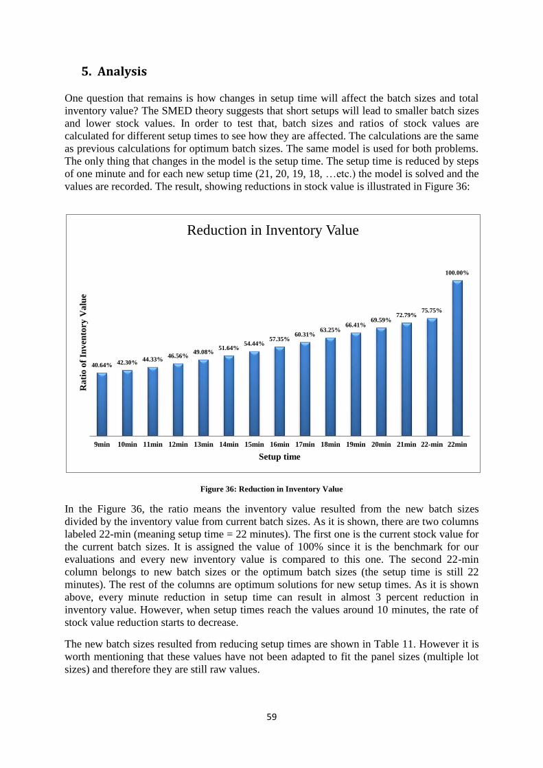
59

5. Analysis

One question that remains is how changes in setup time will affect the batch sizes and total

inventory value? The SMED theory suggests that short setups will lead to smaller batch sizes

and lower stock values. In order to test that, batch sizes and ratios of stock values are

calculated for different setup times to see how they are affected. The calculations are the same

as previous calculations for optimum batch sizes. The same model is used for both problems.

The only thing that changes in the model is the setup time. The setup time is reduced by steps

of one minute and for each new setup time (21, 20, 19, 18, …etc.) the model is solved and the

values are recorded. The result, showing reductions in stock value is illustrated in Figure 36:

Figure 36: Reduction in Inventory Value

In the Figure 36, the ratio means the inventory value resulted from the new batch sizes

divided by the inventory value from current batch sizes. As it is shown, there are two columns

labeled 22-min (meaning setup time = 22 minutes). The first one is the current stock value for

the current batch sizes. It is assigned the value of 100% since it is the benchmark for our

evaluations and every new inventory value is compared to this one. The second 22-min

column belongs to new batch sizes or the optimum batch sizes (the setup time is still 22

minutes). The rest of the columns are optimum solutions for new setup times. As it is shown

above, every minute reduction in setup time can result in almost 3 percent reduction in

inventory value. However, when setup times reach the values around 10 minutes, the rate of

stock value reduction starts to decrease.

The new batch sizes resulted from reducing setup times are shown in Table 11. However it is

worth mentioning that these values have not been adapted to fit the panel sizes (multiple lot

sizes) and therefore they are still raw values.

40.64% 42.30% 44.33%

46.56% 49.08%

51.64% 54.44%

57.35% 60.31%

63.25% 66.41%

69.59% 72.79%

75.75%

100.00%

9min 10min 11min 12min 13min 14min 15min 16min 17min 18min 19min 20min 21min 22-min 22min

Ra

tio

of

Inv

ento

ry V

alu

e

Setup time

Reduction in Inventory Value

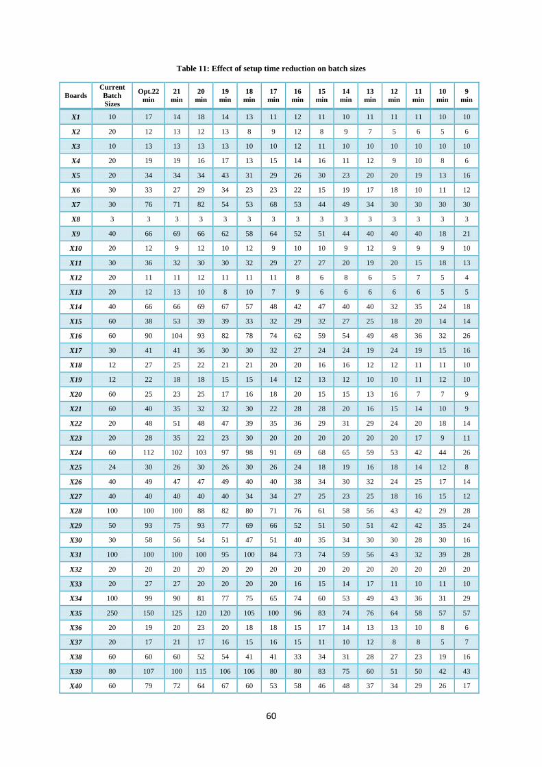
60

Table 11: Effect of setup time reduction on batch sizes

Boards

Current

Batch

Sizes

Opt.22

min

21

min

20

min

19

min

18

min

17

min

16

min

15

min

14

min

13

min

12

min

11

min

10

min

9

min

X1 10 17 14 18 14 13 11 12 11 10 11 11 11 10 10

X2 20 12 13 12 13 8 9 12 8 9 7 5 6 5 6

X3 10 13 13 13 13 10 10 12 11 10 10 10 10 10 10

X4 20 19 19 16 17 13 15 14 16 11 12 9 10 8 6

X5 20 34 34 34 43 31 29 26 30 23 20 20 19 13 16

X6 30 33 27 29 34 23 23 22 15 19 17 18 10 11 12

X7 30 76 71 82 54 53 68 53 44 49 34 30 30 30 30

X8 3 3 3 3 3 3 3 3 3 3 3 3 3 3 3

X9 40 66 69 66 62 58 64 52 51 44 40 40 40 18 21

X10 20 12 9 12 10 12 9 10 10 9 12 9 9 9 10

X11 30 36 32 30 30 32 29 27 27 20 19 20 15 18 13

X12 20 11 11 12 11 11 11 8 6 8 6 5 7 5 4

X13 20 12 13 10 8 10 7 9 6 6 6 6 6 5 5

X14 40 66 66 69 67 57 48 42 47 40 40 32 35 24 18

X15 60 38 53 39 39 33 32 29 32 27 25 18 20 14 14

X16 60 90 104 93 82 78 74 62 59 54 49 48 36 32 26

X17 30 41 41 36 30 30 32 27 24 24 19 24 19 15 16

X18 12 27 25 22 21 21 20 20 16 16 12 12 11 11 10

X19 12 22 18 18 15 15 14 12 13 12 10 10 11 12 10

X20 60 25 23 25 17 16 18 20 15 15 13 16 7 7 9

X21 60 40 35 32 32 30 22 28 28 20 16 15 14 10 9

X22 20 48 51 48 47 39 35 36 29 31 29 24 20 18 14

X23 20 28 35 22 23 30 20 20 20 20 20 20 17 9 11

X24 60 112 102 103 97 98 91 69 68 65 59 53 42 44 26

X25 24 30 26 30 26 30 26 24 18 19 16 18 14 12 8

X26 40 49 47 47 49 40 40 38 34 30 32 24 25 17 14

X27 40 40 40 40 40 34 34 27 25 23 25 18 16 15 12

X28 100 100 100 88 82 80 71 76 61 58 56 43 42 29 28

X29 50 93 75 93 77 69 66 52 51 50 51 42 42 35 24

X30 30 58 56 54 51 47 51 40 35 34 30 30 28 30 16

X31 100 100 100 100 95 100 84 73 74 59 56 43 32 39 28

X32 20 20 20 20 20 20 20 20 20 20 20 20 20 20 20

X33 20 27 27 20 20 20 20 16 15 14 17 11 10 11 10

X34 100 99 90 81 77 75 65 74 60 53 49 43 36 31 29

X35 250 150 125 120 120 105 100 96 83 74 76 64 58 57 57

X36 20 19 20 23 20 18 18 15 17 14 13 13 10 8 6

X37 20 17 21 17 16 15 16 15 11 10 12 8 8 5 7

X38 60 60 60 52 54 41 41 33 34 31 28 27 23 19 16

X39 80 107 100 115 106 106 80 80 83 75 60 51 50 42 43

X40 60 79 72 64 67 60 53 58 46 48 37 34 29 26 17

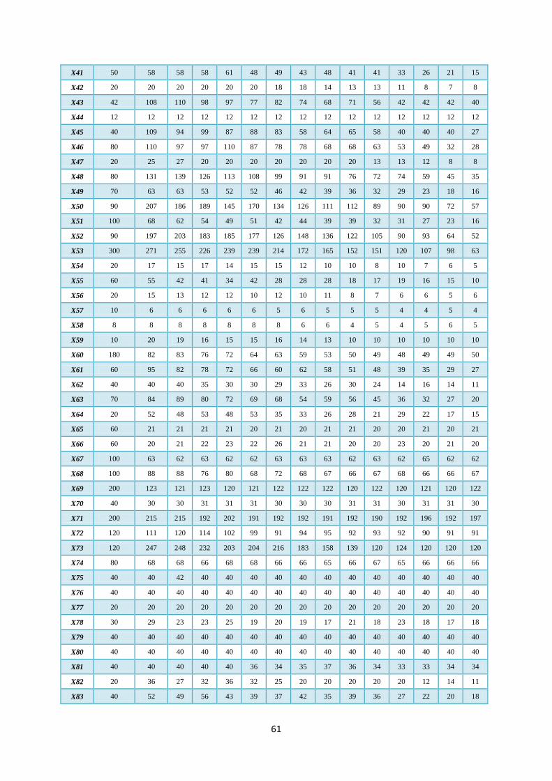
61

X41 50 58 58 58 61 48 49 43 48 41 41 33 26 21 15

X42 20 20 20 20 20 20 18 18 14 13 13 11 8 7 8

X43 42 108 110 98 97 77 82 74 68 71 56 42 42 42 40

X44 12 12 12 12 12 12 12 12 12 12 12 12 12 12 12

X45 40 109 94 99 87 88 83 58 64 65 58 40 40 40 27

X46 80 110 97 97 110 87 78 78 68 68 63 53 49 32 28

X47 20 25 27 20 20 20 20 20 20 20 13 13 12 8 8

X48 80 131 139 126 113 108 99 91 91 76 72 74 59 45 35

X49 70 63 63 53 52 52 46 42 39 36 32 29 23 18 16

X50 90 207 186 189 145 170 134 126 111 112 89 90 90 72 57

X51 100 68 62 54 49 51 42 44 39 39 32 31 27 23 16

X52 90 197 203 183 185 177 126 148 136 122 105 90 93 64 52

X53 300 271 255 226 239 239 214 172 165 152 151 120 107 98 63

X54 20 17 15 17 14 15 15 12 10 10 8 10 7 6 5

X55 60 55 42 41 34 42 28 28 28 18 17 19 16 15 10

X56 20 15 13 12 12 10 12 10 11 8 7 6 6 5 6

X57 10 6 6 6 6 6 5 6 5 5 5 4 4 5 4

X58 8 8 8 8 8 8 8 6 6 4 5 4 5 6 5

X59 10 20 19 16 15 15 16 14 13 10 10 10 10 10 10

X60 180 82 83 76 72 64 63 59 53 50 49 48 49 49 50

X61 60 95 82 78 72 66 60 62 58 51 48 39 35 29 27

X62 40 40 40 35 30 30 29 33 26 30 24 14 16 14 11

X63 70 84 89 80 72 69 68 54 59 56 45 36 32 27 20

X64 20 52 48 53 48 53 35 33 26 28 21 29 22 17 15

X65 60 21 21 21 21 20 21 20 21 21 20 20 21 20 21

X66 60 20 21 22 23 22 26 21 21 20 20 23 20 21 20

X67 100 63 62 63 62 62 63 63 63 62 63 62 65 62 62

X68 100 88 88 76 80 68 72 68 67 66 67 68 66 66 67

X69 200 123 121 123 120 121 122 122 122 120 122 120 121 120 122

X70 40 30 30 31 31 31 30 30 30 31 31 30 31 31 30

X71 200 215 215 192 202 191 192 192 191 192 190 192 196 192 197

X72 120 111 120 114 102 99 91 94 95 92 93 92 90 91 91

X73 120 247 248 232 203 204 216 183 158 139 120 124 120 120 120

X74 80 68 68 66 68 68 66 66 65 66 67 65 66 66 66

X75 40 40 42 40 40 40 40 40 40 40 40 40 40 40 40

X76 40 40 40 40 40 40 40 40 40 40 40 40 40 40 40

X77 20 20 20 20 20 20 20 20 20 20 20 20 20 20 20

X78 30 29 23 23 25 19 20 19 17 21 18 23 18 17 18

X79 40 40 40 40 40 40 40 40 40 40 40 40 40 40 40

X80 40 40 40 40 40 40 40 40 40 40 40 40 40 40 40

X81 40 40 40 40 40 36 34 35 37 36 34 33 33 34 34

X82 20 36 27 32 36 32 25 20 20 20 20 20 12 14 11

X83 40 52 49 56 43 39 37 42 35 39 36 27 22 20 18

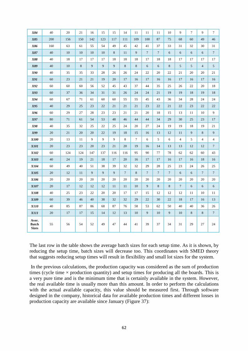
62

X84 40 20 21 16 15 15 14 11 11 11 10 9 7 9 7

X85 200 156 150 142 123 117 111 109 100 87 75 68 60 49 46

X86 160 63 61 55 54 49 45 42 41 37 33 31 32 30 31

X87 40 10 10 10 10 8 11 9 7 7 6 6 6 6 7

X88 40 18 17 17 17 18 18 18 17 18 18 17 17 17 17

X89 40 10 8 9 9 9 8 8 6 6 8 5 5 4 5

X90 40 35 35 33 28 26 26 24 22 20 22 21 20 20 21

X91 60 23 21 21 19 20 17 16 17 16 16 17 16 17 16

X92 60 60 60 56 52 45 43 37 44 35 25 26 22 20 18

X93 60 37 36 34 31 31 26 24 24 21 19 19 18 19 18

X94 60 67 71 61 60 60 55 55 45 43 36 34 28 24 24

X95 40 29 25 23 22 21 21 21 23 22 21 22 23 22 22

X96 60 29 27 28 23 23 21 21 20 18 15 13 11 10 9

X97 80 71 61 54 53 48 46 44 44 34 29 30 25 23 17

X98 40 35 32 25 22 25 24 20 27 24 19 19 18 19 21

X99 20 21 20 20 22 19 18 15 16 13 12 11 9 8 9

X100 20 13 11 9 9 9 8 7 6 5 6 4 5 4 4

X101 20 23 23 20 23 21 20 19 16 14 13 13 12 12 7

X102 60 124 124 147 137 116 116 95 90 77 78 62 62 60 43

X103 40 24 19 21 18 17 20 16 17 17 16 17 16 18 16

X104 60 49 40 51 38 39 32 32 29 28 25 23 24 26 25

X105 20 12 11 9 9 9 7 8 7 7 7 6 6 7 7

X106 20 20 20 20 20 20 20 20 20 20 20 20 20 20 20

X107 20 17 12 12 12 11 11 10 9 8 8 7 6 6 6

X108 40 25 23 22 20 20 17 17 15 12 12 12 11 10 11

X109 60 39 46 40 38 32 32 29 22 30 22 18 17 16 13

X110 40 85 87 86 68 87 76 58 53 62 50 40 40 36 26

X111 20 17 17 15 14 12 13 10 9 10 9 10 8 8 7

Aver.

Batch

Sizes

55 56 54 52 49 47 44 41 39 37 34 31 29 27 24

The last row in the table shows the average batch sizes for each setup time. As it is shown, by

reducing the setup time, batch sizes will decrease too. This coordinates with SMED theory

that suggests reducing setup times will result in flexibility and small lot sizes for the system.

In the previous calculations, the production capacity was considered as the sum of production

times (cycle time × production quantity) and setup times for producing all the boards. This is

a very pure time and is the minimum time that is certainly available in the system. However,

the real available time is usually more than this amount. In order to perform the calculations

with the actual available capacity, this value should be measured first. Through software

designed in the company, historical data for available production times and different losses in

production capacity are available since January (Figure 37):

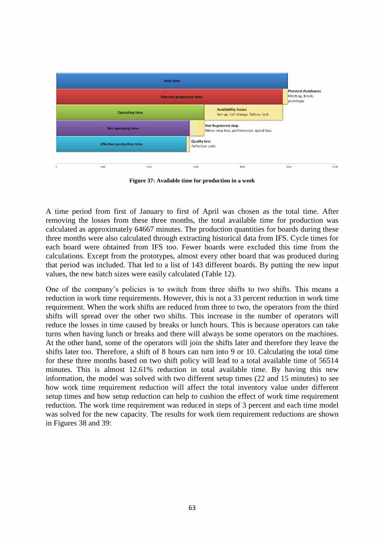
63

Figure 37: Available time for production in a week

A time period from first of January to first of April was chosen as the total time. After

removing the losses from these three months, the total available time for production was

calculated as approximately 64667 minutes. The production quantities for boards during these

three months were also calculated through extracting historical data from IFS. Cycle times for

each board were obtained from IFS too. Fewer boards were excluded this time from the

calculations. Except from the prototypes, almost every other board that was produced during

that period was included. That led to a list of 143 different boards. By putting the new input

values, the new batch sizes were easily calculated (Table 12).

One of the company’s policies is to switch from three shifts to two shifts. This means a

reduction in work time requirements. However, this is not a 33 percent reduction in work time

requirement. When the work shifts are reduced from three to two, the operators from the third

shifts will spread over the other two shifts. This increase in the number of operators will

reduce the losses in time caused by breaks or lunch hours. This is because operators can take

turns when having lunch or breaks and there will always be some operators on the machines.

At the other hand, some of the operators will join the shifts later and therefore they leave the

shifts later too. Therefore, a shift of 8 hours can turn into 9 or 10. Calculating the total time

for these three months based on two shift policy will lead to a total available time of 56514

minutes. This is almost 12.61% reduction in total available time. By having this new

information, the model was solved with two different setup times (22 and 15 minutes) to see

how work time requirement reduction will affect the total inventory value under different

setup times and how setup reduction can help to cushion the effect of work time requirement

reduction. The work time requirement was reduced in steps of 3 percent and each time model

was solved for the new capacity. The results for work tiem requirement reductions are shown

in Figures 38 and 39:

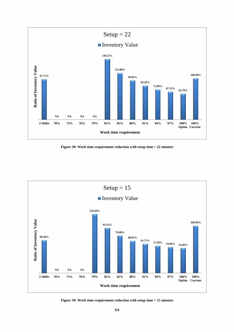
64

Figure 38: Work time requirement reduction with setup time = 22 minutes

Figure 39: Work time requirement reduction with setup time = 15 minutes

97.71%

NA NA NA NA

146.55%

112.88%

94.82%

82.26%

72.89% 67.53%

62.79%

100.00%

2-Shifts 70% 73% 76% 79% 82% 85% 88% 91% 94% 97% 100%

Optim.

100%

Current

Ra

tio

of

Inv

ento

ry V

alu

e

Work time requirement

Setup = 22

Inventory Value

69.49%

NA NA NA

124.64%

95.23%

79.08%

68.05% 61.77%

57.58% 54.96% 52.66%

100.00%

2-Shifts 70% 73% 76% 79% 82% 85% 88% 91% 94% 97% 100%

Optim.

100%

Current

Ra

tio

of

Inv

ento

ry V

alu

e

Work time requirement

Setup = 15

Inventory Value

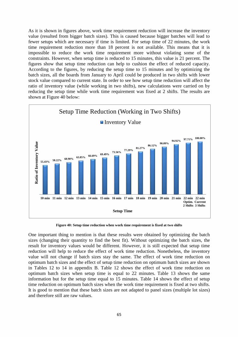
65

As it is shown in figures above, work time requirement reduction will increase the inventory

value (resulted from bigger batch sizes). This is caused because bigger batches will lead to

fewer setups which are necessary if time is limited. For setup time of 22 minutes, the work

time requirement reduction more than 18 percent is not available. This means that it is

impossible to reduce the work time requirement more without violating some of the

constraints. However, when setup time is reduced to 15 minutes, this value is 21 percent. The

figures show that setup time reduction can help to cushion the effect of reduced capacity.

According to the figures, by reducing the setup time to 15 minutes and by optimizing the

batch sizes, all the boards from January to April could be produced in two shifts with lower

stock value compared to current state. In order to see how setup time reduction will affect the

ratio of inventory value (while working in two shifts), new calculations were carried on by

reducing the setup time while work time requirement was fixed at 2 shifts. The results are

shown at Figure 40 below:

Figure 40: Setup time reduction when work time requirement is fixed at two shifts

One important thing to mention is that these results were obtained by optimizing the batch

sizes (changing their quantity to find the best fit). Without optimizing the batch sizes, the

result for inventory values would be different. However, it is still expected that setup time

reduction will help to reduce the effect of work time reduction. Nonetheless, the inventory

value will not change if batch sizes stay the same. The effect of work time reduction on

optimum batch sizes and the effect of setup time reduction on optimum batch sizes are shown

in Tables 12 to 14 in appendix B. Table 12 shows the effect of work time reduction on

optimum batch sizes when setup time is equal to 22 minutes. Table 13 shows the same

information but for the setup time equal to 15 minutes. Table 14 shows the effect of setup

time reduction on optimum batch sizes when the work time requirement is fixed at two shifts.

It is good to mention that these batch sizes are not adapted to panel sizes (multiple lot sizes)

and therefore still are raw values.

55.43% 58.22%

60.90% 63.85%

66.69% 69.49%

73.56% 77.29%

81.27% 86.12%

90.09% 94.92%

97.71% 100.00%

10 min 11 min 12 min 13 min 14 min 15 min 16 min 17 min 18 min 19 min 20 min 21 min 22 min

Optim.

2 Shifts

22 min

Current

3 Shifts

Ra

tio

of

Inv

ento

ry V

alu

e

Setup Time

Setup Time Reduction (Working in Two Shifts)

Inventory Value

66

6. Conclusions and Recommendations

In this thesis project, the problem of finding the optimum batch sizes in a High mix, Low

volume production line was investigated. The case was an SMT line producing a high mix of

different circuit boards in different volumes. The first problem faced throughout the project

was finding an alternative for EOQ method. Economic order quantities, traditionally used in

many firms, were mainly developed for the purpose of inventory management and

purchasing. Within those borders where there is a clear ordering cost including transportation,

insurance and salaries for purchasing staff, the EOQ method makes perfect sense.

Implementing the same principles in a different environment like production can mislead us

enormously. Although many parameters like total demand and inventory holding costs are the

same in both environments, the idea that setup cost is the proper equivalent of ordering cost in

a procurement environment can lead us to many troubles. Setup costs are hard to measure in

many cases and they are usually not fixed values. However, they are widely used in academic

papers as a criterion for calculating the batch sizes. A good alternative for EOQ method was

found to be OR models. By replacing setup cost with setup time and linking that time to the

total available capacity, an OR model can be built that minimizes the inventory value and

finds the optimum batch sizes.

Single Minute Exchange of Die is not a method for calculating batch sizes but it is a powerful

tool for making improvements. It claims that by reducing setup times to less than 10 minutes,

there is no need for specifying batch sizes and one can produce quantities equal to customer

demand. Aside from this claim, the analysis part of this paper shows that reducing setup times

does reduce the average batch sizes. The reduction in inventory value and the increase in

production capacity are among other benefits. It also shows that it can work as a cushion

when work time is reduced. When capacity is limited, it is impossible to perform frequent

setups and produce small lots. However, shortening the setup times can unleash an extra

capacity that was wasted before. Furthermore, the analysis part shows that SMED is at the

heart of a lean production system. Without having short setups, a firm cannot produce in small

batches.

However, working with operators during the thesis work showed that implementing SMED

requires a tremendous amount of soft skills. It is often rejected by the operators, loses its

momentum, management focus turns away and not so before long, it is put aside as one of the

fancy tools of lean that did not work and therefore everyone forgot about it. One way to avoid

that is to build an SMED team that includes both operators and management. This team can

be part of a larger team that is devoted to implement lean company-wide. It is very natural for

the operators to want to prolong setup operations and it is up to management to create the

motivation and devotion in the team and emphasize the importance of the SMED project.

Therefore, management involvement and persistence is critical in the success of any

improvement project.

The analysis part regarding capacity shows that it is possible to reduce the production work

time requirement and batch sizes at the same time. This is possible provided that setup times

are also reduced. Without reducing setup times, reduction in work time requirement will

increase the batch sizes and inventory value. However, the time that is saved by reducing

setup times can cover the reduced work time. In addition, optimizing the batch sizes at the

same time is necessary for reducing the inventory value since inventory value is closely

linked with batch sizes. Based on the analysis part, there is a point where extra reduction in

work time requirement will prevent the system to produce all the customer demand and will

cause serious under production.

67

Both empirical part and analysis part of this report show that optimization techniques in

operations research can lead to significant savings in money. Contrary to that, they are not

widely used in most industries. One further improvement for this work is to develop the OR

model so that it will include panel sizes for each board too. The other improvement is to try to

solve it only with integer values.

The main recommendation for further development of this work is to perform a simulation of

the production line. This simulation should include the SMT line but it can involve other

workstations too. ExtendSim is the best simulation software that comes to mind since it

covers Discrete Event Simulation (DES) topic very well. By having an accurate simulation of

the production line, different scenarios can be tested to see the results. For example, the

answers for optimum batch sizes from MATLAB can be tested to see if they really affect the

inventory value. It is good to see how the system reacts when a large demand arrives or how

changes in setup times affect the stock value or system’s flexibility. ExtendSim is not a

software suitable for optimization specially when there is a wide range of variables or input

data but it is a very strong tool of simulation that can help to verify the optimization results.

One interesting simulation project is to test Shigeo Shingo’s claim that reducing setup times

to less than 10 minutes (For example, three minutes in case of Toyota) can enable a

production system to produce according to customer order quantities.

Finally, another further work can be to look at the setup process of all machines in the SMT

line and try to come up with a procedure that schedules setup tasks in an optimum manner.

68

7. References

Adacher, L. and Cassandras, C. (2013). Lot size optimization in manufacturing systems: The

surrogate method. International Journal of Production Economics, p.1.

Brannen, J. (1992). Mixing methods. 1st ed. Aldershot: Avebury.

Chiu, S., Ting, C. and Chiu, Y. (2007). Optimal production lot sizing with rework, scrap rate,

and service level constraint. Mathematical and Computer Modelling, 46(3), p.535.

Coombs, C. (2008). Printed circuits handbook. 6th ed. New York: McGraw-Hill, pp.40.3-

40.37.

Creswell, J. (2009). Research Design. 1st ed. Thousand Oaks, California: SAGE Publications,

Inc.

Ferradás, P. and Salonitis, K. (2013). Improving changeover time: a tailored SMED approach

for welding Cells. Procedia CIRP, 7, pp.598--603.

Gest, G., Culley, S., McIntosh, R., Mileham, A. and Owen, G. (1995). Review of fast tool

change systems. Computer Integrated Manufacturing Systems, 8(3), pp.205--210.

Goubergen, D. and Landeghem, H. (2002). Rules for integrating fast changeover capabilities

into new equipment design. Robotics and computer-integrated manufacturing, 18(3),

pp.205--214.

Gupta, D. and Magnusson, T. (2005). The capacitated lot-sizing and scheduling problem with

sequence-dependent setup costs and setup times. Computers & Operations Research,

32(4), p.727.

Gutiérrez, J., Sedeño-Noda,, A., Colebrook, M. and Sicilia, J. (2002). A new

characterization for the dynamic lot size problem with bounded inventory. Computers &

Operations Research, 30(3), p.383.

Hillier, F. and Lieberman, G. (2001). Introduction to operations research. 1st ed. Boston:

McGraw-Hill, pp.654, 942-943.

Johansson, B. (1995). Quantitative or qualitative research - or a combination?. 1st ed.

Mo¨lndal: Institutionen fo¨r va°rdla¨rarutbildning, Go¨teborgs univ.

Karmarkar, U. (1987). Lot sizes, lead times and in-process inventories. Management science,

33(3), p.409.

Kim, H. and Hosni, Y. (1998). Manufacturing lot-sizing under MRP II environment: An

improved analytical model & heuristic procedure. Computers & industrial engineering,

35(3), p.423.

Krajewski, L., Ritzman, L. and Malhotra, M. (2007). Operations management. 8th ed. Upper

Saddle River, N.J.: Pearson Prentice Hall, pp.464, 470-473.

Lee, W., Han, J. and Cho, S. (2005). A heuristic algorithm for a multi-product dynamic lot-

sizing and shipping problem. International Journal of Production Economics, 98(2),

p.204.

69

Lindo.com, (2014). LINGO 14.0 - Optimization Modeling Software for Linear, Nonlinear,

and Integer Programming. [online] Available at:

http://www.lindo.com/index.php?option=com_content&view=article&id=2&Itemid=10

[Accessed 14 May. 2014].

Mathworks.se, (2014). Genetic Algorithm – MATLAB - MathWorks Nordic. [online]

Available at: http://www.mathworks.se/discovery/genetic-algorithm.html [Accessed 8

May. 2014].

Mathworks.se, (2014). How the Genetic Algorithm Works - MATLAB & Simulink -

MathWorks Nordic. [online] Available at: http://www.mathworks.se/help/gads/how-the-

genetic-algorithm-works.html [Accessed 8 May. 2014].

Mathworks.se, (2014). MATLAB - The Language of Technical Computing - MathWorks

Nordic. [online] Available at: http://www.mathworks.se/products/matlab/ [Accessed 14

May. 2014].

Mathworks.se, (2014). Optimization of Non-smooth Objective Function - MATLAB &

Simulink Example - MathWorks Nordic. [online] Available at:

http://www.mathworks.se/help/gads/examples/optimization-of-non-smooth-objective-

function.html [Accessed 14 May. 2014].

Nye, T., Jewkes, E. and Dilts, D. (2001). Optimal investment in setup reduction in

manufacturing systems with WIP inventories. European Journal of Operational

Research, 135(1), pp.128--141.

O-digital.com, (2014). Circuit Board-Find Circuit Board supplier|manufacturer|factory in

china.. [online] Available at: http://www.o-digital.com/supplier-

catalogs/2179/2186/Circuit-Board-11.html [Accessed 13 May. 2014].

Pcbfabrication.com, (2014). PCB Quantity. [online] Available at:

http://www.pcbfabrication.com/PCB-fabrication/pcb_Quantity.asp [Accessed 14 May.

2014].

Pinedo, M. (2005). Planning and scheduling in manufacturing and services. 1st ed. New

York, NY: Springer, pp.383-384.

Rader, D. (2010). Deterministic operations research. 1st ed. Hoboken, N.J.: John Wiley &

Sons, Inc., pp.159-160.

Salonen, K. (2008). Setup Optimization in High-Mix Surface Mount PCB Assembly. Ph. D.

University of Turku.

Schemeleva, K., Delorme, X., Dolgui, A. and Grimaud, F. (2012). Multi-product sequencing

and lot-sizing under uncertainties: A memetic algorithm. Engineering Applications of

Artificial Intelligence, 25(8), p.1598.

Sherali, H., Goubergen, D. and Landeghem, H. (2008). A quantitative approach for

scheduling activities to reduce set-up in multiple machine lines. European Journal of

Operational Research, 187(3), pp.1224--1237.

Shingo, S. (1985). A revolution in manufacturing. 1st ed. Cambridge, Massachusetts and

Norwalk, Connecticut: Productivity, pp.12-30.

70

Silver, E., Pyke, D. and Peterson, R. (1998). Inventory management and production planning

and scheduling. 3rd ed. New York: Wiley, pp.46-47.

Vargas, V. (2009). An optimal solution for the stochastic version of the Wagner--Whitin

dynamic lot-size model. European Journal of Operational Research, 198(2), p.447.

Wang, K., Wee, H., Gao, S. and Chung, S. (2005). Production and inventory control with

chaotic demands. Omega, 33(2), p.97.

Westermo.com, (2014). Westermo - Industrial networking solutions, industrial ethernet

switches and routers. [online] Available at: http://www.westermo.com/ [Accessed 24

Apr. 2014].

Yin, R. (2003). Case study research. 1st ed. Thousand Oaks, Calif.: Sage Publications.

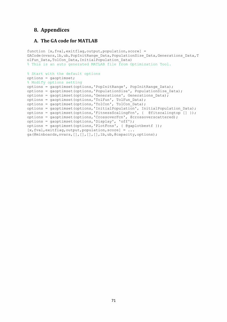
71

8. Appendices

A. The GA code for MATLAB

function [x,fval,exitflag,output,population,score] =

GACode(nvars,lb,ub,PopInitRange_Data,PopulationSize_Data,Generations_Data,T

olFun_Data,TolCon_Data,InitialPopulation_Data) % This is an auto generated MATLAB file from Optimization Tool.

% Start with the default options options = gaoptimset; % Modify options setting options = gaoptimset(options,'PopInitRange', PopInitRange_Data); options = gaoptimset(options,'PopulationSize', PopulationSize_Data); options = gaoptimset(options,'Generations', Generations_Data); options = gaoptimset(options,'TolFun', TolFun_Data); options = gaoptimset(options,'TolCon', TolCon_Data); options = gaoptimset(options,'InitialPopulation', InitialPopulation_Data); options = gaoptimset(options,'FitnessScalingFcn', { @fitscalingtop [] }); options = gaoptimset(options,'CrossoverFcn', @crossoverscattered); options = gaoptimset(options,'Display', 'off'); options = gaoptimset(options,'PlotFcns', { @gaplotbestf }); [x,fval,exitflag,output,population,score] = ... ga(@minboards,nvars,[],[],[],[],lb,ub,@capacity,options);

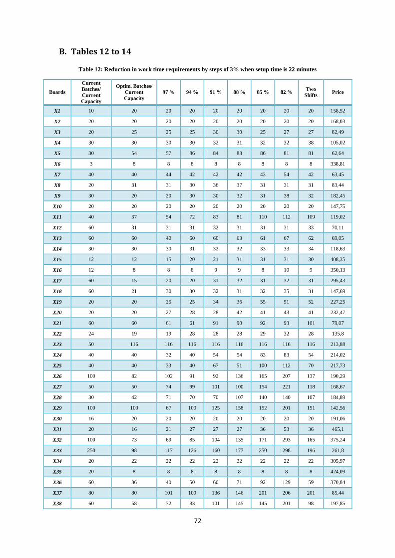
72

B. Tables 12 to 14

Table 12: Reduction in work time requirements by steps of 3% when setup time is 22 minutes

Boards

Current

Batches/

Current

Capacity

Optim. Batches/

Current

Capacity

97 % 94 % 91 % 88 % 85 % 82 % Two

Shifts Price

X1 10 20 20 20 20 20 20 20 20 158,52

X2 20 20 20 20 20 20 20 20 20 168,03

X3 20 25 25 25 30 30 25 27 27 82,49

X4 30 30 30 30 32 31 32 32 38 105,02

X5 30 54 57 86 84 83 86 81 81 62,64

X6 3 8 8 8 8 8 8 8 8 338,81

X7 40 40 44 42 42 42 43 54 42 63,45

X8 20 31 31 30 36 37 31 31 31 83,44

X9 30 20 20 30 30 32 31 38 32 182,45

X10 20 20 20 20 20 20 20 20 20 147,75

X11 40 37 54 72 83 81 110 112 109 119,02

X12 60 31 31 31 32 31 31 31 33 70,11

X13 60 60 40 60 60 63 61 67 62 69,05

X14 30 30 30 31 32 32 33 33 34 118,63

X15 12 12 15 20 21 31 31 31 30 408,35

X16 12 8 8 8 9 9 8 10 9 350,13

X17 60 15 20 20 31 32 31 32 31 295,43

X18 60 21 30 30 32 31 32 35 31 147,69

X19 20 20 25 25 34 36 55 51 52 227,25

X20 20 20 27 28 28 42 41 43 41 232,47

X21 60 60 61 61 91 90 92 93 101 79,07

X22 24 19 19 28 28 28 29 32 28 135,8

X23 50 116 116 116 116 116 116 116 116 213,88

X24 40 40 32 40 54 54 83 83 54 214,02

X25 40 40 33 40 67 51 100 112 70 217,73

X26 100 82 102 91 92 136 165 207 137 190,29

X27 50 50 74 99 101 100 154 221 118 168,67

X28 30 42 71 70 70 107 140 140 107 184,89

X29 100 100 67 100 125 158 152 201 151 142,56

X30 16 20 20 20 20 20 20 20 20 191,06

X31 20 16 21 27 27 27 36 53 36 465,1

X32 100 73 69 85 104 135 171 293 165 375,24

X33 250 98 117 126 160 177 250 298 196 261,8

X34 20 22 22 22 22 22 22 22 22 305,97

X35 20 8 8 8 8 8 8 8 8 424,09

X36 60 36 40 50 60 71 92 129 59 370,84

X37 80 80 101 100 136 146 201 206 201 85,44

X38 60 58 72 83 101 145 145 201 98 197,85

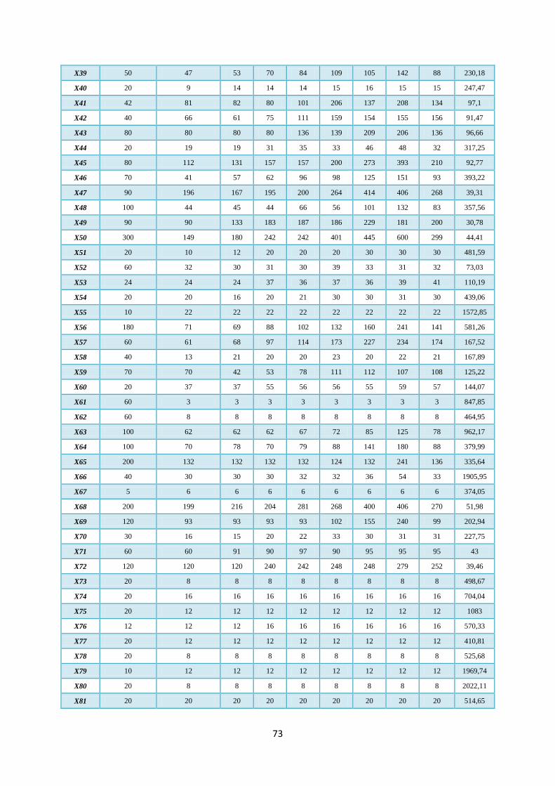
73

X39 50 47 53 70 84 109 105 142 88 230,18

X40 20 9 14 14 14 15 16 15 15 247,47

X41 42 81 82 80 101 206 137 208 134 97,1

X42 40 66 61 75 111 159 154 155 156 91,47

X43 80 80 80 80 136 139 209 206 136 96,66

X44 20 19 19 31 35 33 46 48 32 317,25

X45 80 112 131 157 157 200 273 393 210 92,77

X46 70 41 57 62 96 98 125 151 93 393,22

X47 90 196 167 195 200 264 414 406 268 39,31

X48 100 44 45 44 66 56 101 132 83 357,56

X49 90 90 133 183 187 186 229 181 200 30,78

X50 300 149 180 242 242 401 445 600 299 44,41

X51 20 10 12 20 20 20 30 30 30 481,59

X52 60 32 30 31 30 39 33 31 32 73,03

X53 24 24 24 37 36 37 36 39 41 110,19

X54 20 20 16 20 21 30 30 31 30 439,06

X55 10 22 22 22 22 22 22 22 22 1572,85

X56 180 71 69 88 102 132 160 241 141 581,26

X57 60 61 68 97 114 173 227 234 174 167,52

X58 40 13 21 20 20 23 20 22 21 167,89

X59 70 70 42 53 78 111 112 107 108 125,22

X60 20 37 37 55 56 56 55 59 57 144,07

X61 60 3 3 3 3 3 3 3 3 847,85

X62 60 8 8 8 8 8 8 8 8 464,95

X63 100 62 62 62 67 72 85 125 78 962,17

X64 100 70 78 70 79 88 141 180 88 379,99

X65 200 132 132 132 132 124 132 241 136 335,64

X66 40 30 30 30 32 32 36 54 33 1905,95

X67 5 6 6 6 6 6 6 6 6 374,05

X68 200 199 216 204 281 268 400 406 270 51,98

X69 120 93 93 93 93 102 155 240 99 202,94

X70 30 16 15 20 22 33 30 31 31 227,75

X71 60 60 91 90 97 90 95 95 95 43

X72 120 120 120 240 242 248 248 279 252 39,46

X73 20 8 8 8 8 8 8 8 8 498,67

X74 20 16 16 16 16 16 16 16 16 704,04

X75 20 12 12 12 12 12 12 12 12 1083

X76 12 12 12 16 16 16 16 16 16 570,33

X77 20 12 12 12 12 12 12 12 12 410,81

X78 20 8 8 8 8 8 8 8 8 525,68

X79 10 12 12 12 12 12 12 12 12 1969,74

X80 20 8 8 8 8 8 8 8 8 2022,11

X81 20 20 20 20 20 20 20 20 20 514,65

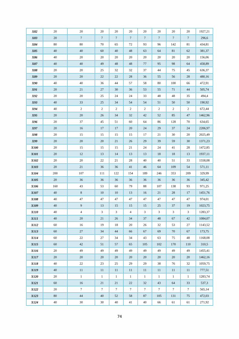
74

X82 20 20 20 20 20 20 20 20 20 1927,21

X83 20 7 7 7 7 7 7 7 7 296,6

X84 80 80 70 65 72 93 96 142 81 434,81

X85 40 40 60 40 48 63 64 81 62 381,37

X86 40 20 20 20 20 20 20 20 20 156,06

X87 40 40 49 48 48 77 95 98 64 458,89

X88 20 20 25 32 32 37 44 75 45 636,37

X89 20 20 22 22 28 36 55 56 28 480,16

X90 40 40 36 44 57 58 80 100 66 472,91

X91 20 21 27 30 36 53 55 71 44 505,74

X92 20 20 25 24 24 33 48 48 35 494,4

X93 40 33 25 34 54 54 51 50 50 190,92

X94 40 2 2 2 2 2 2 2 2 672,44

X95 20 20 26 34 32 42 52 85 47 1462,96

X96 20 37 45 51 60 64 86 128 70 634,65

X97 20 16 17 17 20 24 29 37 24 2206,97

X98 20 15 15 15 15 17 21 30 20 2025,49

X99 20 20 20 21 26 29 39 59 30 1371,23

X100 20 15 15 15 21 24 24 41 28 1472,85

X101 20 12 13 14 13 13 18 18 13 1937,11

X102 20 20 22 21 28 40 40 51 33 1558,08

X103 20 21 36 36 41 46 64 109 54 571,11

X104 200 107 111 122 154 189 246 353 209 329,99

X105 20 36 36 36 36 36 36 36 36 345,42

X106 160 43 53 60 79 88 107 138 93 971,25

X107 40 8 10 10 13 16 21 28 17 1451,76

X108 40 47 47 47 47 47 47 47 47 974,01

X109 40 9 13 15 15 15 25 37 19 1023,75

X110 40 4 3 3 4 3 3 3 3 1283,37

X111 40 20 21 26 34 37 48 67 42 1084,07

X112 60 16 19 18 20 26 32 53 27 1143,52

X113 60 27 34 44 66 67 69 70 67 173,75

X114 60 22 27 34 34 43 63 75 48 1168,08

X115 60 42 51 57 65 105 102 170 110 310,5

X116 20 49 49 49 49 49 49 49 49 1455,41

X117 20 20 20 20 20 20 20 20 20 1462,16

X118 40 22 23 25 29 29 38 76 32 1059,75

X119 40 11 11 11 11 11 11 11 11 777,51

X120 20 1 1 1 1 1 1 1 1 1283,74

X121 60 16 21 21 22 32 43 64 33 537,3

X122 20 7 7 7 7 7 7 7 7 565,14

X123 80 44 40 52 58 87 105 131 75 472,03

X124 40 30 30 40 41 40 66 61 61 271,92

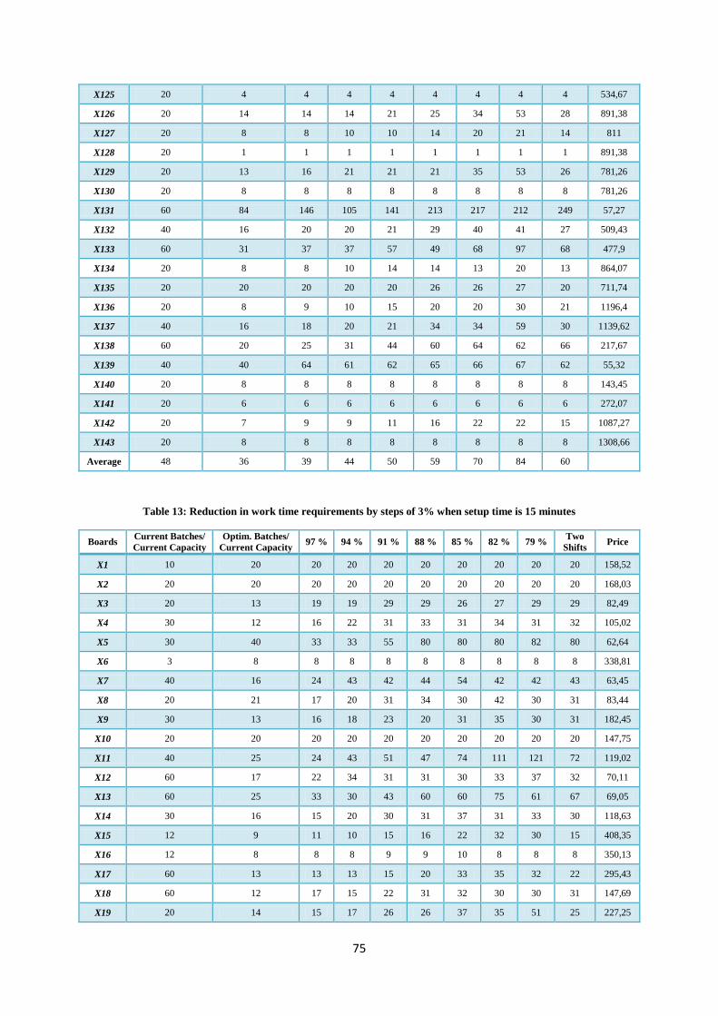
75

X125 20 4 4 4 4 4 4 4 4 534,67

X126 20 14 14 14 21 25 34 53 28 891,38

X127 20 8 8 10 10 14 20 21 14 811

X128 20 1 1 1 1 1 1 1 1 891,38

X129 20 13 16 21 21 21 35 53 26 781,26

X130 20 8 8 8 8 8 8 8 8 781,26

X131 60 84 146 105 141 213 217 212 249 57,27

X132 40 16 20 20 21 29 40 41 27 509,43

X133 60 31 37 37 57 49 68 97 68 477,9

X134 20 8 8 10 14 14 13 20 13 864,07

X135 20 20 20 20 20 26 26 27 20 711,74

X136 20 8 9 10 15 20 20 30 21 1196,4

X137 40 16 18 20 21 34 34 59 30 1139,62

X138 60 20 25 31 44 60 64 62 66 217,67

X139 40 40 64 61 62 65 66 67 62 55,32

X140 20 8 8 8 8 8 8 8 8 143,45

X141 20 6 6 6 6 6 6 6 6 272,07

X142 20 7 9 9 11 16 22 22 15 1087,27

X143 20 8 8 8 8 8 8 8 8 1308,66

Average 48 36 39 44 50 59 70 84 60

Table 13: Reduction in work time requirements by steps of 3% when setup time is 15 minutes

Boards Current Batches/

Current Capacity

Optim. Batches/

Current Capacity 97 % 94 % 91 % 88 % 85 % 82 % 79 %

Two

Shifts Price

X1 10 20 20 20 20 20 20 20 20 20 158,52

X2 20 20 20 20 20 20 20 20 20 20 168,03

X3 20 13 19 19 29 29 26 27 29 29 82,49

X4 30 12 16 22 31 33 31 34 31 32 105,02

X5 30 40 33 33 55 80 80 80 82 80 62,64

X6 3 8 8 8 8 8 8 8 8 8 338,81

X7 40 16 24 43 42 44 54 42 42 43 63,45

X8 20 21 17 20 31 34 30 42 30 31 83,44

X9 30 13 16 18 23 20 31 35 30 31 182,45

X10 20 20 20 20 20 20 20 20 20 20 147,75

X11 40 25 24 43 51 47 74 111 121 72 119,02

X12 60 17 22 34 31 31 30 33 37 32 70,11

X13 60 25 33 30 43 60 60 75 61 67 69,05

X14 30 16 15 20 30 31 37 31 33 30 118,63

X15 12 9 11 10 15 16 22 32 30 15 408,35

X16 12 8 8 8 9 9 10 8 8 8 350,13

X17 60 13 13 13 15 20 33 35 32 22 295,43

X18 60 12 17 15 22 31 32 30 30 31 147,69

X19 20 14 15 17 26 26 37 35 51 25 227,25

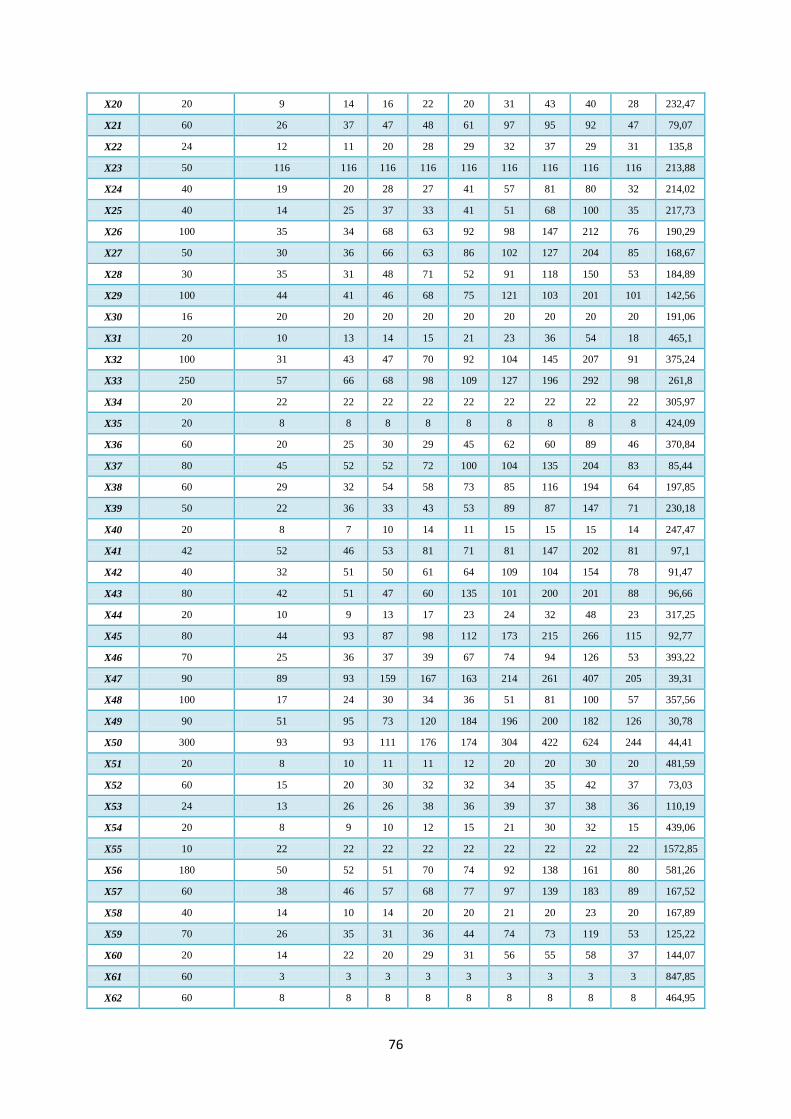
76

X20 20 9 14 16 22 20 31 43 40 28 232,47

X21 60 26 37 47 48 61 97 95 92 47 79,07

X22 24 12 11 20 28 29 32 37 29 31 135,8

X23 50 116 116 116 116 116 116 116 116 116 213,88

X24 40 19 20 28 27 41 57 81 80 32 214,02

X25 40 14 25 37 33 41 51 68 100 35 217,73

X26 100 35 34 68 63 92 98 147 212 76 190,29

X27 50 30 36 66 63 86 102 127 204 85 168,67

X28 30 35 31 48 71 52 91 118 150 53 184,89

X29 100 44 41 46 68 75 121 103 201 101 142,56

X30 16 20 20 20 20 20 20 20 20 20 191,06

X31 20 10 13 14 15 21 23 36 54 18 465,1

X32 100 31 43 47 70 92 104 145 207 91 375,24

X33 250 57 66 68 98 109 127 196 292 98 261,8

X34 20 22 22 22 22 22 22 22 22 22 305,97

X35 20 8 8 8 8 8 8 8 8 8 424,09

X36 60 20 25 30 29 45 62 60 89 46 370,84

X37 80 45 52 52 72 100 104 135 204 83 85,44

X38 60 29 32 54 58 73 85 116 194 64 197,85

X39 50 22 36 33 43 53 89 87 147 71 230,18

X40 20 8 7 10 14 11 15 15 15 14 247,47

X41 42 52 46 53 81 71 81 147 202 81 97,1

X42 40 32 51 50 61 64 109 104 154 78 91,47

X43 80 42 51 47 60 135 101 200 201 88 96,66

X44 20 10 9 13 17 23 24 32 48 23 317,25

X45 80 44 93 87 98 112 173 215 266 115 92,77

X46 70 25 36 37 39 67 74 94 126 53 393,22

X47 90 89 93 159 167 163 214 261 407 205 39,31

X48 100 17 24 30 34 36 51 81 100 57 357,56

X49 90 51 95 73 120 184 196 200 182 126 30,78

X50 300 93 93 111 176 174 304 422 624 244 44,41

X51 20 8 10 11 11 12 20 20 30 20 481,59

X52 60 15 20 30 32 32 34 35 42 37 73,03

X53 24 13 26 26 38 36 39 37 38 36 110,19

X54 20 8 9 10 12 15 21 30 32 15 439,06

X55 10 22 22 22 22 22 22 22 22 22 1572,85

X56 180 50 52 51 70 74 92 138 161 80 581,26

X57 60 38 46 57 68 77 97 139 183 89 167,52

X58 40 14 10 14 20 20 21 20 23 20 167,89

X59 70 26 35 31 36 44 74 73 119 53 125,22

X60 20 14 22 20 29 31 56 55 58 37 144,07

X61 60 3 3 3 3 3 3 3 3 3 847,85

X62 60 8 8 8 8 8 8 8 8 8 464,95

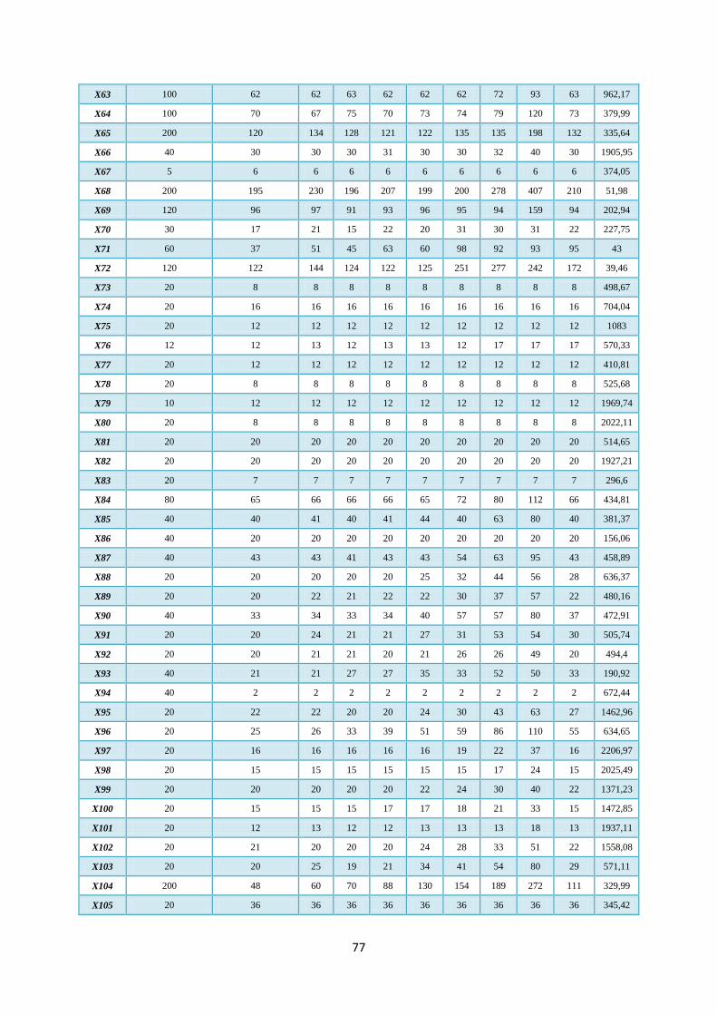
77

X63 100 62 62 63 62 62 62 72 93 63 962,17

X64 100 70 67 75 70 73 74 79 120 73 379,99

X65 200 120 134 128 121 122 135 135 198 132 335,64

X66 40 30 30 30 31 30 30 32 40 30 1905,95

X67 5 6 6 6 6 6 6 6 6 6 374,05

X68 200 195 230 196 207 199 200 278 407 210 51,98

X69 120 96 97 91 93 96 95 94 159 94 202,94

X70 30 17 21 15 22 20 31 30 31 22 227,75

X71 60 37 51 45 63 60 98 92 93 95 43

X72 120 122 144 124 122 125 251 277 242 172 39,46

X73 20 8 8 8 8 8 8 8 8 8 498,67

X74 20 16 16 16 16 16 16 16 16 16 704,04

X75 20 12 12 12 12 12 12 12 12 12 1083

X76 12 12 13 12 13 13 12 17 17 17 570,33

X77 20 12 12 12 12 12 12 12 12 12 410,81

X78 20 8 8 8 8 8 8 8 8 8 525,68

X79 10 12 12 12 12 12 12 12 12 12 1969,74

X80 20 8 8 8 8 8 8 8 8 8 2022,11

X81 20 20 20 20 20 20 20 20 20 20 514,65

X82 20 20 20 20 20 20 20 20 20 20 1927,21

X83 20 7 7 7 7 7 7 7 7 7 296,6

X84 80 65 66 66 66 65 72 80 112 66 434,81

X85 40 40 41 40 41 44 40 63 80 40 381,37

X86 40 20 20 20 20 20 20 20 20 20 156,06

X87 40 43 43 41 43 43 54 63 95 43 458,89

X88 20 20 20 20 20 25 32 44 56 28 636,37

X89 20 20 22 21 22 22 30 37 57 22 480,16

X90 40 33 34 33 34 40 57 57 80 37 472,91

X91 20 20 24 21 21 27 31 53 54 30 505,74

X92 20 20 21 21 20 21 26 26 49 20 494,4

X93 40 21 21 27 27 35 33 52 50 33 190,92

X94 40 2 2 2 2 2 2 2 2 2 672,44

X95 20 22 22 20 20 24 30 43 63 27 1462,96

X96 20 25 26 33 39 51 59 86 110 55 634,65

X97 20 16 16 16 16 16 19 22 37 16 2206,97

X98 20 15 15 15 15 15 15 17 24 15 2025,49

X99 20 20 20 20 20 22 24 30 40 22 1371,23

X100 20 15 15 15 17 17 18 21 33 15 1472,85

X101 20 12 13 12 12 13 13 13 18 13 1937,11

X102 20 21 20 20 20 24 28 33 51 22 1558,08

X103 20 20 25 19 21 34 41 54 80 29 571,11

X104 200 48 60 70 88 130 154 189 272 111 329,99

X105 20 36 36 36 36 36 36 36 36 36 345,42

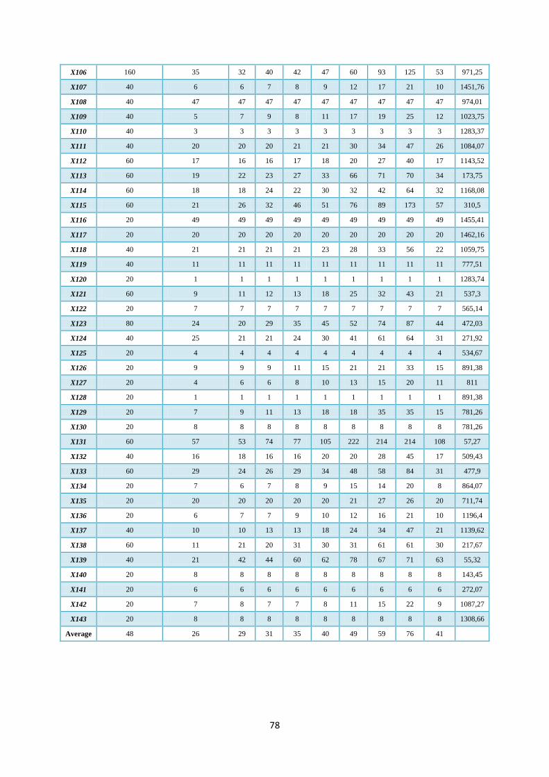
78

X106 160 35 32 40 42 47 60 93 125 53 971,25

X107 40 6 6 7 8 9 12 17 21 10 1451,76

X108 40 47 47 47 47 47 47 47 47 47 974,01

X109 40 5 7 9 8 11 17 19 25 12 1023,75

X110 40 3 3 3 3 3 3 3 3 3 1283,37

X111 40 20 20 20 21 21 30 34 47 26 1084,07

X112 60 17 16 16 17 18 20 27 40 17 1143,52

X113 60 19 22 23 27 33 66 71 70 34 173,75

X114 60 18 18 24 22 30 32 42 64 32 1168,08

X115 60 21 26 32 46 51 76 89 173 57 310,5

X116 20 49 49 49 49 49 49 49 49 49 1455,41

X117 20 20 20 20 20 20 20 20 20 20 1462,16

X118 40 21 21 21 21 23 28 33 56 22 1059,75

X119 40 11 11 11 11 11 11 11 11 11 777,51

X120 20 1 1 1 1 1 1 1 1 1 1283,74

X121 60 9 11 12 13 18 25 32 43 21 537,3

X122 20 7 7 7 7 7 7 7 7 7 565,14

X123 80 24 20 29 35 45 52 74 87 44 472,03

X124 40 25 21 21 24 30 41 61 64 31 271,92

X125 20 4 4 4 4 4 4 4 4 4 534,67

X126 20 9 9 9 11 15 21 21 33 15 891,38

X127 20 4 6 6 8 10 13 15 20 11 811

X128 20 1 1 1 1 1 1 1 1 1 891,38

X129 20 7 9 11 13 18 18 35 35 15 781,26

X130 20 8 8 8 8 8 8 8 8 8 781,26

X131 60 57 53 74 77 105 222 214 214 108 57,27

X132 40 16 18 16 16 20 20 28 45 17 509,43

X133 60 29 24 26 29 34 48 58 84 31 477,9

X134 20 7 6 7 8 9 15 14 20 8 864,07

X135 20 20 20 20 20 20 21 27 26 20 711,74

X136 20 6 7 7 9 10 12 16 21 10 1196,4

X137 40 10 10 13 13 18 24 34 47 21 1139,62

X138 60 11 21 20 31 30 31 61 61 30 217,67

X139 40 21 42 44 60 62 78 67 71 63 55,32

X140 20 8 8 8 8 8 8 8 8 8 143,45

X141 20 6 6 6 6 6 6 6 6 6 272,07

X142 20 7 8 7 7 8 11 15 22 9 1087,27

X143 20 8 8 8 8 8 8 8 8 8 1308,66

Average 48 26 29 31 35 40 49 59 76 41

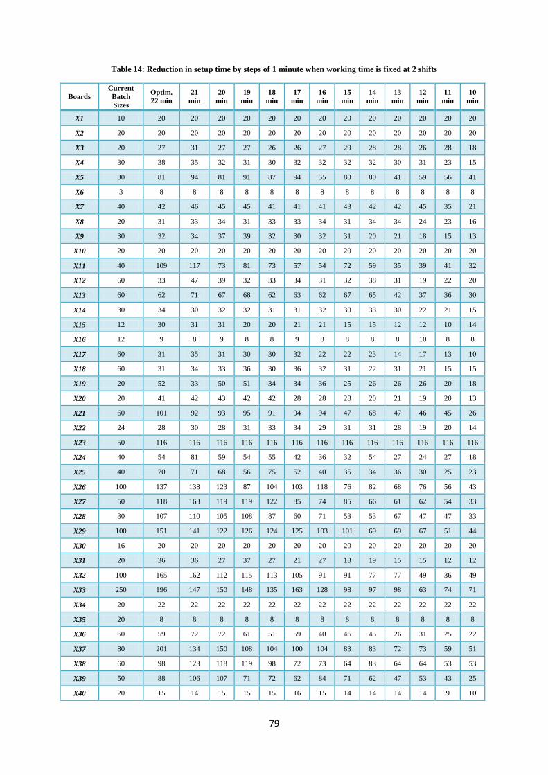
79

Table 14: Reduction in setup time by steps of 1 minute when working time is fixed at 2 shifts

Boards

Current

Batch

Sizes

Optim.

22 min

21

min

20

min

19

min

18

min

17

min

16

min

15

min

14

min

13

min

12

min

11

min

10

min

X1 10 20 20 20 20 20 20 20 20 20 20 20 20 20

X2 20 20 20 20 20 20 20 20 20 20 20 20 20 20

X3 20 27 31 27 27 26 26 27 29 28 28 26 28 18

X4 30 38 35 32 31 30 32 32 32 32 30 31 23 15

X5 30 81 94 81 91 87 94 55 80 80 41 59 56 41

X6 3 8 8 8 8 8 8 8 8 8 8 8 8 8

X7 40 42 46 45 45 41 41 41 43 42 42 45 35 21

X8 20 31 33 34 31 33 33 34 31 34 34 24 23 16

X9 30 32 34 37 39 32 30 32 31 20 21 18 15 13

X10 20 20 20 20 20 20 20 20 20 20 20 20 20 20

X11 40 109 117 73 81 73 57 54 72 59 35 39 41 32

X12 60 33 47 39 32 33 34 31 32 38 31 19 22 20

X13 60 62 71 67 68 62 63 62 67 65 42 37 36 30

X14 30 34 30 32 32 31 31 32 30 33 30 22 21 15

X15 12 30 31 31 20 20 21 21 15 15 12 12 10 14

X16 12 9 8 9 8 8 9 8 8 8 8 10 8 8

X17 60 31 35 31 30 30 32 22 22 23 14 17 13 10

X18 60 31 34 33 36 30 36 32 31 22 31 21 15 15

X19 20 52 33 50 51 34 34 36 25 26 26 26 20 18

X20 20 41 42 43 42 42 28 28 28 20 21 19 20 13

X21 60 101 92 93 95 91 94 94 47 68 47 46 45 26

X22 24 28 30 28 31 33 34 29 31 31 28 19 20 14

X23 50 116 116 116 116 116 116 116 116 116 116 116 116 116

X24 40 54 81 59 54 55 42 36 32 54 27 24 27 18

X25 40 70 71 68 56 75 52 40 35 34 36 30 25 23

X26 100 137 138 123 87 104 103 118 76 82 68 76 56 43

X27 50 118 163 119 119 122 85 74 85 66 61 62 54 33

X28 30 107 110 105 108 87 60 71 53 53 67 47 47 33

X29 100 151 141 122 126 124 125 103 101 69 69 67 51 44

X30 16 20 20 20 20 20 20 20 20 20 20 20 20 20

X31 20 36 36 27 37 27 21 27 18 19 15 15 12 12

X32 100 165 162 112 115 113 105 91 91 77 77 49 36 49

X33 250 196 147 150 148 135 163 128 98 97 98 63 74 71

X34 20 22 22 22 22 22 22 22 22 22 22 22 22 22

X35 20 8 8 8 8 8 8 8 8 8 8 8 8 8

X36 60 59 72 72 61 51 59 40 46 45 26 31 25 22

X37 80 201 134 150 108 104 100 104 83 83 72 73 59 51

X38 60 98 123 118 119 98 72 73 64 83 64 64 53 53

X39 50 88 106 107 71 72 62 84 71 62 47 53 43 25

X40 20 15 14 15 15 15 16 15 14 14 14 14 9 10

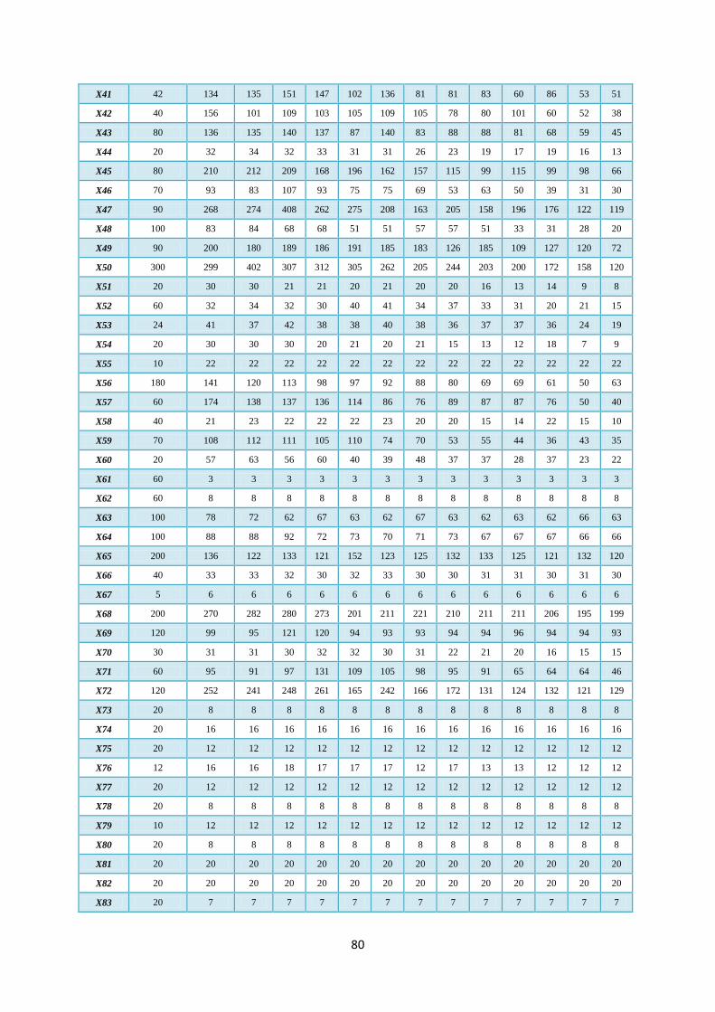
80

X41 42 134 135 151 147 102 136 81 81 83 60 86 53 51

X42 40 156 101 109 103 105 109 105 78 80 101 60 52 38

X43 80 136 135 140 137 87 140 83 88 88 81 68 59 45

X44 20 32 34 32 33 31 31 26 23 19 17 19 16 13

X45 80 210 212 209 168 196 162 157 115 99 115 99 98 66

X46 70 93 83 107 93 75 75 69 53 63 50 39 31 30

X47 90 268 274 408 262 275 208 163 205 158 196 176 122 119

X48 100 83 84 68 68 51 51 57 57 51 33 31 28 20

X49 90 200 180 189 186 191 185 183 126 185 109 127 120 72

X50 300 299 402 307 312 305 262 205 244 203 200 172 158 120

X51 20 30 30 21 21 20 21 20 20 16 13 14 9 8

X52 60 32 34 32 30 40 41 34 37 33 31 20 21 15

X53 24 41 37 42 38 38 40 38 36 37 37 36 24 19

X54 20 30 30 30 20 21 20 21 15 13 12 18 7 9

X55 10 22 22 22 22 22 22 22 22 22 22 22 22 22

X56 180 141 120 113 98 97 92 88 80 69 69 61 50 63

X57 60 174 138 137 136 114 86 76 89 87 87 76 50 40

X58 40 21 23 22 22 22 23 20 20 15 14 22 15 10

X59 70 108 112 111 105 110 74 70 53 55 44 36 43 35

X60 20 57 63 56 60 40 39 48 37 37 28 37 23 22

X61 60 3 3 3 3 3 3 3 3 3 3 3 3 3

X62 60 8 8 8 8 8 8 8 8 8 8 8 8 8

X63 100 78 72 62 67 63 62 67 63 62 63 62 66 63

X64 100 88 88 92 72 73 70 71 73 67 67 67 66 66

X65 200 136 122 133 121 152 123 125 132 133 125 121 132 120

X66 40 33 33 32 30 32 33 30 30 31 31 30 31 30

X67 5 6 6 6 6 6 6 6 6 6 6 6 6 6

X68 200 270 282 280 273 201 211 221 210 211 211 206 195 199

X69 120 99 95 121 120 94 93 93 94 94 96 94 94 93

X70 30 31 31 30 32 32 30 31 22 21 20 16 15 15

X71 60 95 91 97 131 109 105 98 95 91 65 64 64 46

X72 120 252 241 248 261 165 242 166 172 131 124 132 121 129

X73 20 8 8 8 8 8 8 8 8 8 8 8 8 8

X74 20 16 16 16 16 16 16 16 16 16 16 16 16 16

X75 20 12 12 12 12 12 12 12 12 12 12 12 12 12

X76 12 16 16 18 17 17 17 12 17 13 13 12 12 12

X77 20 12 12 12 12 12 12 12 12 12 12 12 12 12

X78 20 8 8 8 8 8 8 8 8 8 8 8 8 8

X79 10 12 12 12 12 12 12 12 12 12 12 12 12 12

X80 20 8 8 8 8 8 8 8 8 8 8 8 8 8

X81 20 20 20 20 20 20 20 20 20 20 20 20 20 20

X82 20 20 20 20 20 20 20 20 20 20 20 20 20 20

X83 20 7 7 7 7 7 7 7 7 7 7 7 7 7

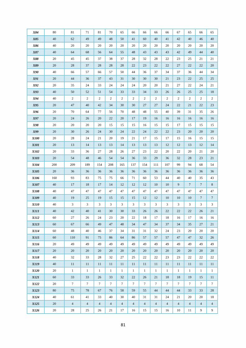
81

X84 80 81 71 81 70 65 66 66 66 66 67 65 66 65

X85 40 62 49 49 48 50 41 60 40 41 42 40 46 40

X86 40 20 20 20 20 20 20 20 20 20 20 20 20 20

X87 40 64 68 56 64 55 48 43 43 43 42 49 44 40

X88 20 45 45 37 38 37 28 32 28 22 23 25 21 21

X89 20 28 37 28 28 28 22 23 22 22 27 22 22 20

X90 40 66 57 66 57 50 44 36 37 34 37 36 44 34

X91 20 44 36 37 43 31 30 30 30 21 23 22 25 25

X92 20 35 24 33 24 24 24 20 20 21 27 22 24 21

X93 40 50 52 51 54 33 33 34 33 26 26 25 25 18

X94 40 2 2 2 2 2 2 2 2 2 2 2 2 2

X95 20 47 40 42 34 30 30 27 27 24 22 21 22 23

X96 20 70 64 77 56 70 48 48 55 40 39 31 35 26

X97 20 24 26 20 22 20 17 19 16 16 16 16 16 16

X98 20 20 20 20 15 15 15 16 15 15 17 15 15 15

X99 20 30 26 24 30 24 22 24 22 22 23 20 20 20

X100 20 28 24 21 20 19 21 17 15 17 15 16 15 15

X101 20 13 14 13 13 14 13 13 13 12 12 13 12 14

X102 20 33 36 27 28 26 27 23 22 20 22 20 21 20

X103 20 54 48 46 54 54 36 33 29 36 32 28 23 21

X104 200 209 189 154 208 165 137 154 111 107 99 94 68 54

X105 20 36 36 36 36 36 36 36 36 36 36 36 36 36

X106 160 93 83 75 75 66 71 60 53 44 40 40 35 43

X107 40 17 18 17 14 12 12 12 10 10 9 7 7 8

X108 40 47 47 47 47 47 47 47 47 47 47 47 47 47

X109 40 19 25 19 15 15 15 12 12 10 10 10 7 7

X110 40 3 3 3 3 3 3 3 3 3 3 3 3 3

X111 40 42 40 41 30 30 33 26 26 22 22 22 26 21

X112 60 27 26 24 23 20 22 18 17 18 16 17 16 16

X113 60 67 66 49 47 48 34 47 34 37 34 35 27 21

X114 60 48 40 46 37 34 31 31 32 24 23 20 20 20

X115 60 110 91 75 86 64 86 57 57 57 47 47 32 26

X116 20 49 49 49 49 49 49 49 49 49 49 49 49 49

X117 20 20 20 20 20 20 20 20 20 20 20 20 20 20

X118 40 32 33 28 32 27 25 22 22 23 23 22 22 22

X119 40 11 11 11 11 11 11 11 11 11 11 11 11 11

X120 20 1 1 1 1 1 1 1 1 1 1 1 1 1

X121 60 33 33 26 33 32 22 26 21 18 18 19 15 11

X122 20 7 7 7 7 7 7 7 7 7 7 7 7 7

X123 80 75 78 67 76 58 59 55 44 44 44 33 33 28

X124 40 61 41 33 40 30 40 31 31 24 21 20 20 18

X125 20 4 4 4 4 4 4 4 4 4 4 4 4 4

X126 20 28 25 26 21 17 16 15 15 16 10 11 9 9

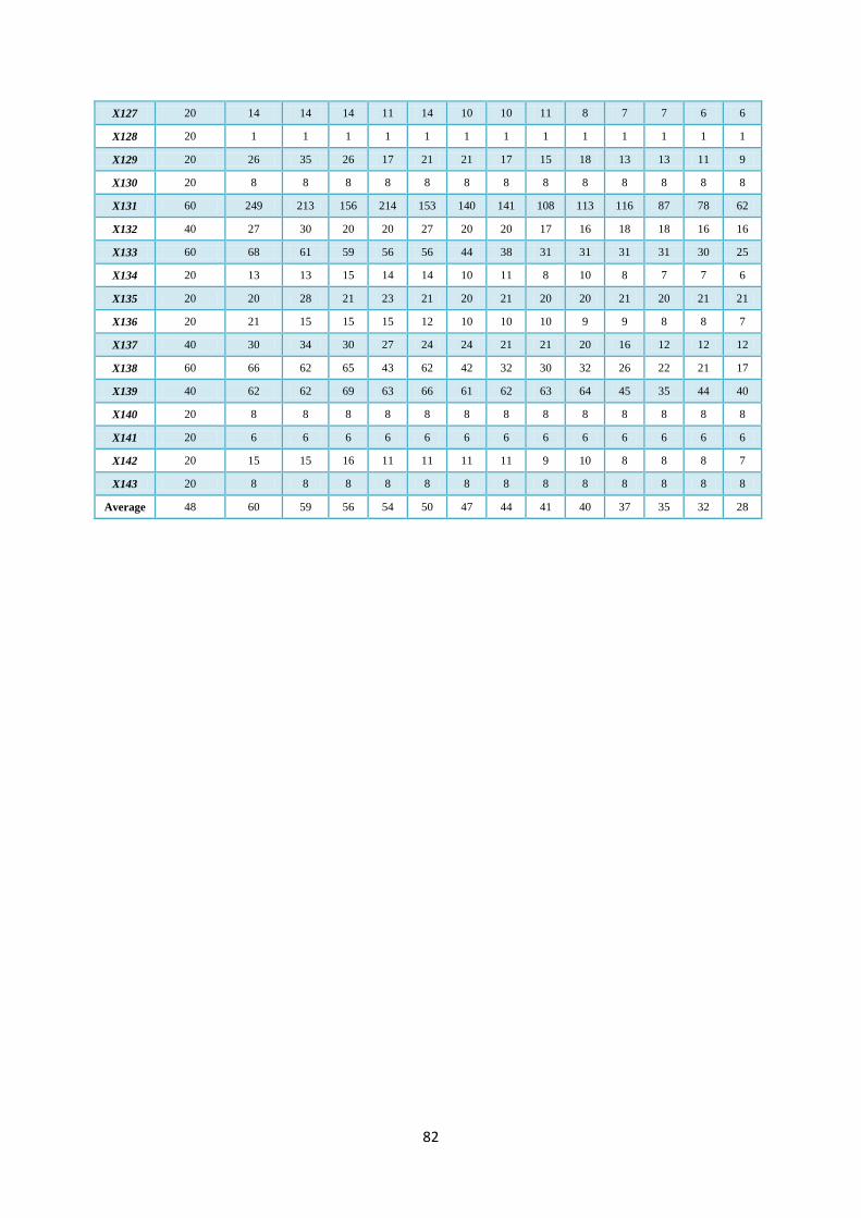
82

X127 20 14 14 14 11 14 10 10 11 8 7 7 6 6

X128 20 1 1 1 1 1 1 1 1 1 1 1 1 1

X129 20 26 35 26 17 21 21 17 15 18 13 13 11 9

X130 20 8 8 8 8 8 8 8 8 8 8 8 8 8

X131 60 249 213 156 214 153 140 141 108 113 116 87 78 62

X132 40 27 30 20 20 27 20 20 17 16 18 18 16 16

X133 60 68 61 59 56 56 44 38 31 31 31 31 30 25

X134 20 13 13 15 14 14 10 11 8 10 8 7 7 6

X135 20 20 28 21 23 21 20 21 20 20 21 20 21 21

X136 20 21 15 15 15 12 10 10 10 9 9 8 8 7

X137 40 30 34 30 27 24 24 21 21 20 16 12 12 12

X138 60 66 62 65 43 62 42 32 30 32 26 22 21 17

X139 40 62 62 69 63 66 61 62 63 64 45 35 44 40

X140 20 8 8 8 8 8 8 8 8 8 8 8 8 8

X141 20 6 6 6 6 6 6 6 6 6 6 6 6 6

X142 20 15 15 16 11 11 11 11 9 10 8 8 8 7

X143 20 8 8 8 8 8 8 8 8 8 8 8 8 8

Average 48 60 59 56 54 50 47 44 41 40 37 35 32 28