Finding active factors from unreplicated fractional factorials utilizing the total time on test (TTT) technique

$Page 1: Finding active factors from unreplicated fractional factorials utilizing the total time on test (TTT) technique$
QUALITY AND RELIABILITY ENGINEERING INTERNATIONAL

Qual. Reliab. Engng. Int.15: 191–203 (1999)

FINDING ACTIVE FACTORS FROM UNREPLICATEDFRACTIONAL FACTORIALS UTILIZING THE TOTAL TIME ON

TEST (TTT) TECHNIQUE

PIA SANDVIK WIKLUND 1∗ AND BO BERGMAN2

1Division of Quality Technology and Statistics, Lule˚a University of Technology, SE-97187 Lule˚a, Sweden2Division of Quality Technology and Management, Linköping University, SE-58183 Linköping, Sweden

SUMMARYMuch research has been devoted to improving the process of identifying active factors from designed experiments.Generally, the proposed methods rely on an estimate of the experimental error. Here we present a method basedon the TTT (total time on test) plot, where the scaled TTT transform enables an evaluation of the contrastsindependently of the experimental error. The method can be separated into two parts. The first part consists ofa transformed TTT plot for a visual evaluation of data. The second part is more formal and utilizes the cumulativeTTT statistic for testing the significance of contrasts. A simulation study shows the power of the method comparedwith competing methods. Five data sets are used to show that the conclusions drawn are consistent with thoseobtained using other suggested methods. Copyright 1999 John Wiley & Sons, Ltd.

KEY WORDS: unreplicated fractional factorials; total time on test; Laplace test; active factors; identification

1. INTRODUCTION

In industry, design of experiments in general andunreplicated fractional factorial designs in particularare gaining increased interest [1,2]. Therefore it isimportant to find simple and adequate methods tosupport engineers in their analysis of unreplicatedfractional factorial experiments. The (half [3]) normalplot introduced by Daniel [4], is an excellent tool forsimple and illustrative analysis of design experiments;however, it is informal and subjective. A largenumber of more or less formal methods have beensuggested [5–13]. These methods are, unfortunately,not especially illustrative, as in general they are notsupported by any graphical analyses. It is the aim ofthis paper to suggest a general idea for combining agraphical technique with a supporting formal test. Thegeneral idea based on statistical life length analysistechniques is made precise by suggesting a specificprocedure for identification of active contrasts from anunreplicated fractional factorial experiment.

We will utilize the fact that under commonassumptions, squared contrasts from factorial designs

∗Correspondence to: P. Sandvik Wiklund, Division of QualityTechnology and Statistics, Lule˚a University of Technology, SE-97187 Lulea, Sweden. Email: [email protected]/grant sponsor: Design of Experiments and Robust DesignNetwork of Swedish Industrial Firms.

corresponding to inert contrasts are positive randomvariables with a cumulative distribution function,which is known except for a scale parameter.For positive random variables, life length analysismethods become available. In this paper we shallutilize the total time on test (TTT) plotting technique,first introduced by Barlow and Campo [14] andfurther studied by e.g. Bergman and Klefsjö [15];see also Reference [16] and references cited therein.Especially, we shall suggest the utilization of amodification of the Laplace test, one of the oldestknown statistical test procedures; see e.g. Chapter 6 inReference [17]. For ease of reference we have includeda brief description of the TTT plotting procedure, thecorresponding TTT transform and the cumulative TTTstatistic in AppendixI.

Let yi , i = 1, . . . , m + 1, be the observed valuesfrom an unreplicated fractional factorial experimentwith independent, identically normally distributederrors with mean zero. The contrastsci correspondingto inert contrasts are observations from anN(0, σ 2)

random variable, whereσ 2 is the variance of acontrast. Thus the corresponding squared contrastszi = c2

i are observations from a scaled chi-squared distribution with one degree of freedom,σ 2χ2(1). Now, if all squared contrasts correspondto inert contrasts, then the TTT plotting procedure

CCC 0748–8017/99/030191–13$17.50 Received 4 January 1998Copyright 1999 John Wiley & Sons, Ltd. Revised 1 November 1998

192 P. SANDVIK WIKLUND AND B. BERGMAN

will result in a TTT plot which should be closeto the corresponding scaled TTT transform of aχ2(1) distribution. If some of the contrasts correspondto active contrasts, then the empirical cumulativedistribution function (CDF) of all squared contrastsshould be more ‘tail-heavy’ than that of aχ2(1)

distribution. We thus have a visual support foridentifying active contrasts.

Of course, there are a number of ways in whichwe could define tail-heaviness. Here we shall assumethat it means that the distribution is DFR (decreasingfailure rate) with respect toχ2(1). Of course, othercriteria would lead to other test statistics. However, inthis paper we shall restrict ourselves to this specialcase. It relates to the same type of alternatives asthe ones suggested by Box and Meyer [5], who infact a priori suggest a mixture distribution of thecontrasts; that would lead to a mixture distribution ofthe squared contrasts which is DFR with respect to theoriginalχ2(1) distribution [18]. A natural statistic formeasuring DFR-ness is the cumulative TTT statistic,which is closely related to the Laplace test statistic.

In this paper we shall exploit the above idea andcompare it with two procedures suggested earlier; forease of reference these two competing procedureswill be briefly discussed in the next section. InSection3 we shall describe the TTT plotting procedureapplied to an example. In Section4 we illustratethe use of the cumulative TTT statistic and, by wayof simulations, calculate its probability limits underthe null hypothesis that there are no active contrasts;see also AppendixII . In Section 5 we suggest aprocedure for identifying active contrasts based on thecumulative TTT statistic. In Section6 we give someillustrations showing that our suggested procedure iscomparable with other procedures suggested earlier.The study is deepened in a separate paper [19]. Finally,in Section7 we discuss the procedure and draw someconclusions; especially, we note that there are a lot ofpossibilities for utilizing the basic idea in this paper toderive new, possibly improved, identification routines.

2. TWO PROCEDURES FOR FINDING ACTIVEFACTORS

Lenth [8] proposed a simple analysis techniquewhere the estimated standard deviations0 =1.5 median|ci |, i = 1, . . . , m, is used as an initialestimate. The pseudo standard error (PSE) is definedas PSE= 1.5 median|ci |, where the contrasts includedare those larger than 2.5s0 PSE and an approximate95% confidence interval is given by ME± ci ; herethe margin of error (ME) is obtained through ME=

t0.975,d PSE, whered = m/3. In order to reducethe risk of ME leading to a false conclusion, Lenthdefines the outer confidence limits in terms of thesimultaneous margin of error (SME) as SME= tγ,d

PSE, whereγ = (1 + 0.951/m)/2. Contrasts outsidethe outer confidence limits,±SME, are consideredactive and contrasts inside the inner confidence limits,±ME, are declared inert. Contrasts between the innerand outer confidence limits are subject to uncertaintyand can be declared either active or inert. Lenthalso suggests a graph containing the inner and outerconfidence limits in which the estimated contrasts canbe plotted directly.

Venter and Steel [13] proposed a method based onthe ratios

Wi = Ui+1

/(1

i

i∑j=1

U2j

)1/2

, i = 1, . . . , m − 1

whereU(1) ≤ U(2) ≤ · · · ≤ U(m) are the orderedstatistics of the estimated contrasts|c1|, |c2|, . . . , |cm |.Let Fi be the marginal distribution function ofWi

under the null hypothesis H0 that all contrasts areinert, i.e. Fi (x) = Pr(Ti ≤ x | H0). A p-valueassociated withWi is defined asPi = 1 − Fi (Wi );furthermore, they defineSl = min{Pi : l ≤ i ≤m − 1}, where 1 ≤ l ≤ m − 1. Under H0 thedistribution of Sl can be calculated. Their test rejectsH0 if Sl ≤ sl(α), wheresl(α) is theαth quantile ofthe distribution ofSl . Let q be the first index such thatq ≥ l and Pq ≤ sl (α); then q is the number of inertcontrasts. The distribution of the probabilityPi can besimulated using an arbitrarily large sample of randomvectors, each withm components that areN(0, 1), as areference. The quantilessl (α) can be obtained throughsimulation and are provided in Reference [13] for thecasesm = 7, 15 and 31. Venter and Steel recommendthat with an assumption of effect sparsity,l is chosenlarge; otherwise a smaller value is more suitable. Theirgeneral recommendation is to choose a value ofl thatunderestimates the number of true inert contrasts.

3. UTILIZING TTT PLOTTING

The scaled TTT transform enables evaluation of thecontrasts independent ofσ 2. The squared contrastszi corresponding to zero-mean contrasts areσ 2χ2(1)

distributed. The ordered squared contrastsz(i) can belooked upon in the same way as the ordered sample offailure times and can thus be studied in a TTT plot. Ifthe contrasts are generated by random noise, the TTTplot of the squared ordered contrastsz(i) should followthe scaled TTT transform of theχ2(1) distribution

Copyright 1999 John Wiley & Sons, Ltd. Qual. Reliab. Engng. Int.15: 191–203 (1999)

ACTIVE FACTORS FROM UNREPLICATED FRACTIONAL FACTORIALS 193

Table 1. Design matrix, responses and confounding pattern for foundry data

EF BF AF EL EO BO BLDE DF AB AE AD BD BE DL AH BH DO DH AL AO

No. A B D E F H L O y

1 − − + − + + − − + + − + − − + 262.42 − − + − + + − + − − + − + + − 262.73 − − + + − − + − + + − − + + − 259.44 − − + + − − + + − − + + − − + 261.85 − + − − + − + − + − + + − + − 265.66 − + − − + − + + − + − − + − + 264.67 − + − + − + − − + − + − + − + 263.38 − + − + − + − + − + − + − + − 263.59 + − − − − + + − − + + + + − − 260.4

10 + − − − − + + + + − − − − + + 260.611 + − − + + − − − − + + − − + + 261.112 + − − + + − − + + − − + + − − 262.613 + + + − − − − − − − − + + + + 264.614 + + + − − − − + + + + − − − − 264.715 + + + + + + + − − − − − − − − 265.416 + + + + + + + + + + + + + + + 265.2

presented in Figure12 in Appendix I. Otherwise, ifthere are contrasts distinguishable from noise, the TTTplot is more DFR than the scaled TTT transform of theχ2(1) distribution. To make the comparison simpler,we suggest a further transformation. The TTT plotis transformed by plottingϕ(i/n) againstϕn. Hereϕ(i/n) is the scaled TTT transform of theχ2(1)

distribution according to equation (5) in AppendixI,with u = i/n for i = 1, . . . , n, and ϕn is Ti/Tn ,whereTi is the total test time at failure timex( j ) andTn is the total test time. In the transformed TTT plota data set including only inert contrasts approachesthe unit square diagonal. Note that the purpose of thistransformation is to make visual evaluation simpler.

The proposed TTT plot procedure is illustrated onan experiment conducted by the Swedish FoundryAssociation in a research project together with theDivision of Quality Technology and Management atLinkoping University. The purpose of the experimentwas to identify influential factors on the presence ofpores in a brake cylinder. The experiment is presentedin Reference [20].

The design for the foundry experiment is a 28–4

fractional factorial with resolution III; see Table1. Theletters correspond to the following factors: A, furnacetemperature; B, casting pressure; D, air cooling andcleaning; E, vacuum; F, starting point for secondphase; H, plunger velocity in first phase; L, plungervelocity in second phase; O, cycle time.

The two-factor interactions considered importanta priori are shown in bold type. Three response

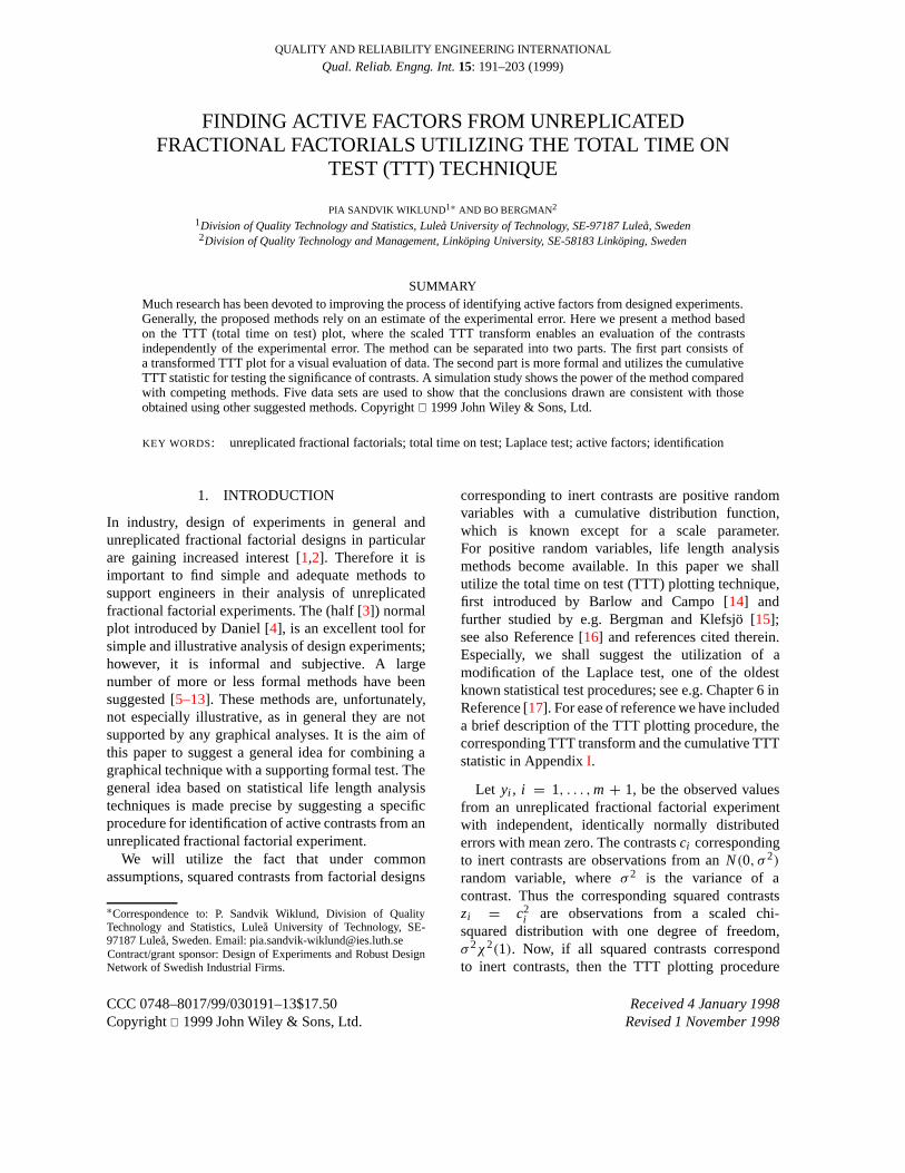
Figure 1. Normal probability plot of contrasts from foundry data

variables, the amount of pores graded from 1 to10, the density and the weight, were measured.In this paper, one of the response variables, theweight y (see Table1), is presented and analysed. Anormal probability plot of the estimated contrasts ispresented in Figure1. The conclusion from the normalprobability plot is that factor B can be consideredactive. Further, it is uncertain whether factor E is activeor not.

The ordered squared contrasts together withϕ(i/15) and Ti/T15 are presented in Table2. Thecorresponding transformed TTT plot is presented inFigure2 and it is obvious that data consist of variationdistinguishable from noise. The example is furtherstudied in Section5.



Table 2. Analysis of foundry data with TTT plot technique

Factor Squared contrast ϕ(i/15) Ti/T15

EL 0.0014 0.0067 0.0015O 0.0077 0.0257 0.0076F 0.0127 0.0556 0.0122A 0.0264 0.0953 0.0238DO 0.0452 0.1438 0.0383BE 0.0564 0.2003 0.0463BO+AL 0.0827 0.2642 0.0629AO 0.0977 0.3350 0.0713D 0.1702 0.4121 0.1070H 0.1914 0.4951 0.1160L 0.2889 0.5841 0.1503EF 0.3164 0.6787 0.1580EO+BH 0.4389 0.7789 0.1839E 1.9952 0.8853 0.4029B 10.4814 1.0000 1.0000

Figure 2. Transformed TTT plot for foundry data

4. A MODIFIED LAPLACE TEST

There is, however, also a need for a more formalway to judge whether data have been generated bysomething other than noise, i.e. if data include activecontrasts. This is achieved by studying the cumulativeTTT statistic

Vn =n−1∑i=1

Ti/Tn

=n−1∑i=1

∑ij=1(n − j + 1)(z( j ) − z( j−1)∑n

j=1(n − j + 1)(z( j ) − z( j−1))(1)

wherez(1) ≤ z(2) ≤ · · · ≤ z(n) are the ordered squaredcontrasts.

In order to determine whether or not there are anycontrasts distinguishable from noise, a significance

Table 3. Lower percentiles forun

Percentiles forunn 10% 5% 2.5% 1% 0.5%

2 1.14 1.17 1.18 1.18 1.183 1.31 1.49 1.58 1.63 1.654 1.31 1.57 1.74 1.87 1.935 1.29 1.59 1.80 2.00 2.096 1.28 1.58 1.83 2.06 2.197 1.28 1.59 1.84 2.11 2.268 1.28 1.59 1.85 2.13 2.319 1.28 1.60 1.86 2.15 2.34

10 1.28 1.60 1.87 2.16 2.3611 1.28 1.60 1.87 2.16 2.3712 1.28 1.60 1.88 2.18 2.3813 1.28 1.60 1.88 2.20 2.3914 1.28 1.60 1.88 2.20 2.4115 1.28 1.61 1.89 2.21 2.40∞ 1.28 1.64 1.96 2.33 2.56

test is performed. The test uses the quantity

un = −(Vn − E[Vn])/√

Var[Vn] (2)

where E[Vn] and Var[Vn] are obtained throughformulae (9) and (10) found from simulation; seeAppendix II . According to Moore [21], Vn isasymptotically normally distributed and thusun isasymptotically N(0, 1). Here we considerVn asapproximately normally distributed forn > 15, whichseems to be a reasonable assumption for our purposes.

The significance level forun exceeding somevalue u0 is determined by Pr(un > u0). Whenn ≤ 15,un should be compared with the standardizedlower percentiles in Table3, which also includes thepercentiles whenn → ∞, i.e. the normal distribution.The test is one-sided, since if the data material consistsof active contrasts, it is the lower percentiles ofVn thatare of interest. A large observedun indicates a heavytail, i.e. some of the contrasts are large, comparedwith the assumedχ2(1) distribution. The percentilesof un, assuming that there are no active contrasts, aregiven in Table3, which essentially is obtained fromsimulations; see AppendixII .

5. IDENTIFICATION OF ACTIVE CONTRASTS

Preferably, the analysis is entered by visuallyevaluating the transformed TTT plot of allz(i)

to determine whether the contrasts are affected bysomething other than random variation. Thereafterthe same evaluation is made through a significancetest by comparingun with the chosen critical valuein Table 3. If data are determined to include activecontrasts, the largest squared contrast is excluded



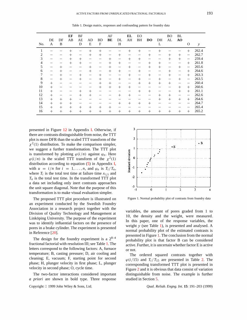
Figure 3. Transformed TTT plots for foundry data

Table 4. Estimated values for TTT plot technique

EstimatedVn un p(%) Factor deemed active

1.28 3.17 <0.5 B3.27 1.30 ≈10 None

from the data. The reduced data set is plotted in thetransformed TTT plot, which is evaluated visually,and a new significance test is conducted forun−1to find additional active contrasts. The procedure isrepeated until the remaining data are judged as beinggenerated by noise. The contrasts removed can thus beconsidered active.

Consider the foundry data studied in Section3. Thetransformed TTT plot presented on the left in Figure3is first studied. The clear indication of DFR-ness ofthe data material indicates that there might be activecontrasts. The corresponding cumulative TTT statisticV15 is calculated through formula(1) and givesu15 ≈3.17 whosep-value is less than 0.5%; see Table4. Theconclusion drawn is thus that factor B is active.

Factor B is thus excluded from the data material,and the plot on the right in Figure3 shows the reduceddata material plotted in the transformed TTT plot.The plot indicates some DFR-ness with respect to theχ2(1) distribution, but it is not statistically significant(p ≈ 10%); see Table4. Hence the TTT plotprocedure gives the same indications as the normalprobability plot.

We have compared with the results of theprocedures of Lenth [8] and Venter and Steel [13]for α = 5%. In Lenth’s method this is equal toSME = 4.024 PSE, and for Venter and Steel the least

number of contrasts assumed inert is set tol = 3and the critical value is chosen as 0.001. The reasonsfor the choices are given in Section6.1. Lenth’sproposed method gives results that are consistent withthe conclusions above. The inner confidence limits aregiven as±ME = ±1.11 and the outer confidencelimits as±SME = ±1.81. Hence factor B is outsideSME and is deemed clearly active. Factor E liesbetween ME and SME and is therefore in the zone ofuncertainty and can be deemed both active and inert.Venter and Steel come to the same conclusion that onlyfactor B is indicated as active.

6. ILLUSTRATIONS

6.1. A simulation study

The performances of the methods of Lenth [8] andVenter and Steel [13] are compared with the proposedmethod through a simulation study. Daniel [3]and Birnbaum [22] performed small simulationstudies including only one active contrast. Generally,the earlier performed simulation studies includemore than one active contrast varied in differentpatterns [9,13,23,24]. An extensive simulation studyincluding the TTT plot-based method proposed inthis paper and seven other methods is presented inReference [19]. In that study the number of activecontrasts,r , takes several different values and thenon-null means are varied in a number of differentconfigurations.

Here we have chosen a somewhat differentapproach than earlier simulation studies. The samplingdistributions of the contrastsci are regarded as normalwith mean zero but with different variancesf 2σ 2.Hence the active contrasts are simulated from an



Figure 4. Power plot and difference plot forf = 3

N(0, f 2σ 2) distribution, wheref = 3, . . . , 29, andthe inert contrasts are simulated from anN(0, σ 2)

distribution. We have chosen to setr = 1, 2, . . . , 8for the non-null contrasts, and forr > 1 all theactive contrasts are simulated from the same normaldistribution.

We have studied 16-run effect-saturated fractionalfactorials, i.e.m = 15, and each case has beensimulated 5000 times utilizing the random generatorof Matlab 4.2c.1. The power of the correct selectedactive contrasts,h, has been estimated for each of thecases, while controllingα to be around 5%.

The studied procedures have been automated asclosely as possible to the original description given bythe corresponding authors. The critical values of eachmethod have been chosen to give an error rateα of 5%under the null hypothesis that all contrasts are inert.

In Lenth’s procedure we use SME= t0.885,d PSE,wheret0.885,d = 4.024 form = 15, which accordingto Reference [13] has approximately 95% confidence.The critical value of Venter and Steel is chosen as0.001 instead of 0.0045 as proposed in Table2 inReference [13], as a pilot simulation study indicatedthatαi was far too high. The least number of contrastsassumed inert was set tol = 3.

The left plot in Figure4 shows the power plotsfor the methods studied and the right plot displaysthe difference in power between the proposed methodand the other methods. The two plots indicate that forf = 3 the methods do not identify many of the active

contrasts. The proposed method seems to have higherpower than the methods of Lenth and of Venter andSteel.

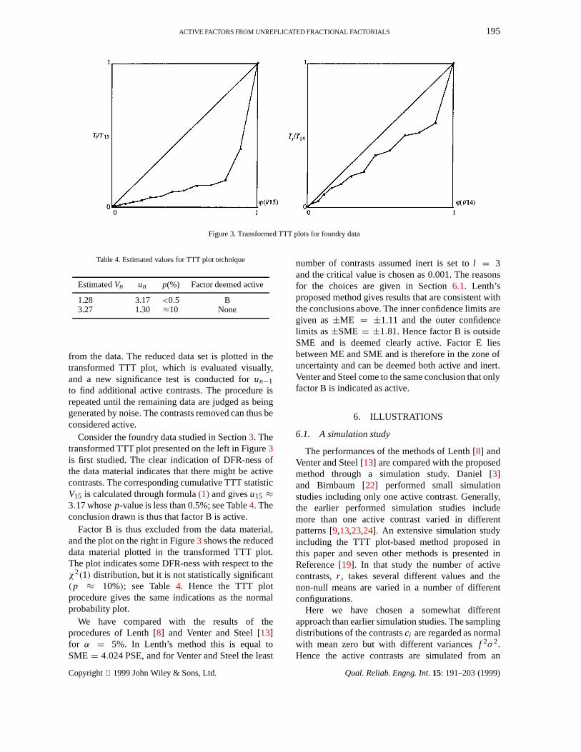
In Figure 5, f is equal to 13 and the power hasincreased in comparison withf = 3. It seems as if thepower is quite similar between methods when effectsparsity is valid, but forr ≥ 7 the proposed methodseems to have lower power than the other methodstested.

The situation seems to be similar whenf = 21;see Figure6. The study indicates that Lenth’s andVenter and Steel’s methods have higher power thanthe proposed method when the assumption of effectsparsity is violated.

The simulation study indicates that the proposedmethod has higher power than the other two methodsunder effect sparsity, i.e. whenr ≤ 6. Thereafter thepower of the method decreases relative to the othermethods tested. The deterioration is probably due tothe characteristics of the cumulative TTT statistic,which acts strangely when there are clusters in thedata.

6.2. Examples

The four examples (Examples I–IV) presented inReference [5] are re-examined here to illustrate theproposed method. The examples have previously beenanalysed with other selection procedures; see e.g.References [12] and [24]. Figure 7 shows normalprobability plots of the four examples.





Table 5 presents the calculatedun for the fourexamples, together with theirp-values, for differentnumbers of contrasts,n. The p-values are found fromTable3.

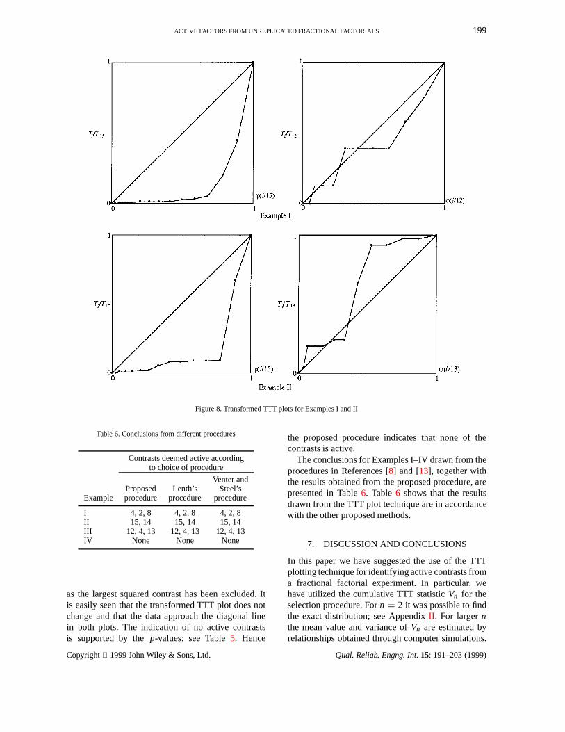
Figure 8 shows the transformed TTT plots forExamples I and II. In the left plot of Example I, allcontrasts are included and it is obvious that the dataconsist of systematic variation, which is supported bythe formal test that has ap-value smaller than 0.5%;see Table5.

In the right plot of Example I the three largestcontrasts have been removed and the data approach thediagonal; thus variability in the data is due to randomvariation, andu12 ≈ 0.72 having ap-value larger than10% supports the indications of the plot. That is, theproposed procedure indicates that contrasts 4, 2 and 8should be deemed active.

For Example II, contrasts 14 and 15 appear to beactive; see the normal probability plot in Figure7, thetransformed TTT plots in Figure8 and Table5. It is



Figure 7. Normal probability plots of data presented in Reference [5]

Table 5. Results from proposed procedure

Example I Example II Example III Example IV

p Active p Active p Active p Activen un (%) i un (%) i un (%) i un (%) i

15 3.66 <0.5 4 3.31 <0.5 15 2.60 <0.5 12 0.74 >10 None14 3.23 <0.5 2 3.01 <0.5 14 2.77 <0.5 413 2.63 <0.5 8 −1.09 >10 None 2.72 <0.5 1312 0.73 >10 None 0.80 −0.25 >10 None

easily seen in the transformed TTT plot to the left inFigure 8 that the data are influenced by systematicvariation, which is verified by ap-value that issmaller than 0.5%. For the remaining 13 contrasts thetransformed TTT plot and the estimatedp-value largerthan 10% indicate only noise; thus the conclusion fromthe proposed procedure is that contrasts 14 and 15 areactive.

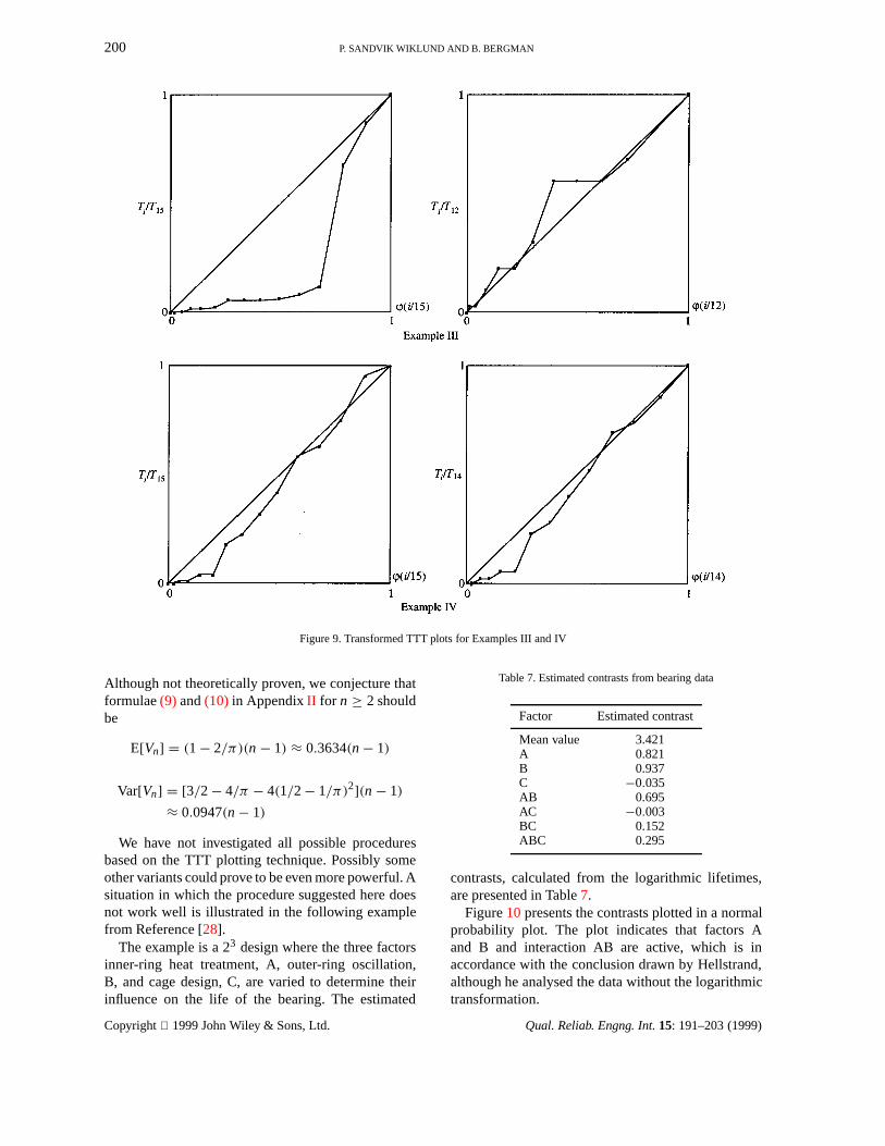
Regarding Example III, the transformed TTT plotsof all contrasts (see Figure9) and the corresponding

p-values (see Table5) indicate that the data includecontrasts that are distinguishable from noise, and thelargest squared contrast is thus excluded from the data.Two more contrasts are excluded until we get thetransformed TTT plot to the right with ap-value largerthan 10%. Hence the proposed procedure indicatesthat contrasts 4, 12 and 13 are active.

Considering Example IV, the transformed TTT plotsare presented in Figure9, where the left plot includesall contrasts and the right plot includes 14 contrasts,



Figure 8. Transformed TTT plots for Examples I and II

Table 6. Conclusions from different procedures

Contrasts deemed active accordingto choice of procedure

Venter andProposed Lenth’s Steel’s

Example procedure procedure procedure

I 4, 2, 8 4, 2, 8 4, 2, 8II 15, 14 15, 14 15, 14III 12, 4, 13 12, 4, 13 12, 4, 13IV None None None

as the largest squared contrast has been excluded. Itis easily seen that the transformed TTT plot does notchange and that the data approach the diagonal linein both plots. The indication of no active contrastsis supported by thep-values; see Table5. Hence

the proposed procedure indicates that none of thecontrasts is active.

The conclusions for Examples I–IV drawn from theprocedures in References [8] and [13], together withthe results obtained from the proposed procedure, arepresented in Table6. Table6 shows that the resultsdrawn from the TTT plot technique are in accordancewith the other proposed methods.

7. DISCUSSION AND CONCLUSIONS

In this paper we have suggested the use of the TTTplotting technique for identifying active contrasts froma fractional factorial experiment. In particular, wehave utilized the cumulative TTT statisticVn for theselection procedure. Forn = 2 it was possible to findthe exact distribution; see AppendixII . For largernthe mean value and variance ofVn are estimated byrelationships obtained through computer simulations.



Figure 9. Transformed TTT plots for Examples III and IV

Although not theoretically proven, we conjecture thatformulae(9) and(10) in AppendixII for n ≥ 2 shouldbe

E[Vn] = (1 − 2/π)(n − 1) ≈ 0.3634(n − 1)

Var[Vn] = [3/2 − 4/π − 4(1/2 − 1/π)2](n − 1)

≈ 0.0947(n − 1)

We have not investigated all possible proceduresbased on the TTT plotting technique. Possibly someother variants could prove to be even more powerful. Asituation in which the procedure suggested here doesnot work well is illustrated in the following examplefrom Reference [28].

The example is a 23 design where the three factorsinner-ring heat treatment, A, outer-ring oscillation,B, and cage design, C, are varied to determine theirinfluence on the life of the bearing. The estimated

Table 7. Estimated contrasts from bearing data

Factor Estimated contrast

Mean value 3.421A 0.821B 0.937C −0.035AB 0.695AC −0.003BC 0.152ABC 0.295

contrasts, calculated from the logarithmic lifetimes,are presented in Table7.

Figure10 presents the contrasts plotted in a normalprobability plot. The plot indicates that factors Aand B and interaction AB are active, which is inaccordance with the conclusion drawn by Hellstrand,although he analysed the data without the logarithmictransformation.



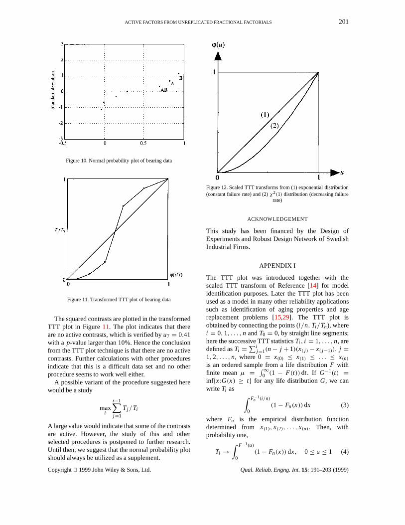
Figure 10. Normal probability plot of bearing data

Figure 11. Transformed TTT plot of bearing data

The squared contrasts are plotted in the transformedTTT plot in Figure11. The plot indicates that thereare no active contrasts, which is verified byu7 = 0.41with a p-value larger than 10%. Hence the conclusionfrom the TTT plot technique is that there are no activecontrasts. Further calculations with other proceduresindicate that this is a difficult data set and no otherprocedure seems to work well either.

A possible variant of the procedure suggested herewould be a study

maxi

i−1∑j=1

Tj/Ti

A large value would indicate that some of the contrastsare active. However, the study of this and otherselected procedures is postponed to further research.Until then, we suggest that the normal probability plotshould always be utilized as a supplement.

Figure 12. Scaled TTT transforms from (1) exponential distribution(constant failure rate) and (2)χ2(1) distribution (decreasing failure

rate)

ACKNOWLEDGEMENT

This study has been financed by the Design ofExperiments and Robust Design Network of SwedishIndustrial Firms.

APPENDIX I

The TTT plot was introduced together with thescaled TTT transform of Reference [14] for modelidentification purposes. Later the TTT plot has beenused as a model in many other reliability applicationssuch as identification of aging properties and agereplacement problems [15,29]. The TTT plot isobtained by connecting the points (i/n, Ti/Tn), wherei = 0, 1, . . . , n andT0 = 0, by straight line segments;here the successive TTT statisticsTi , i = 1, . . . , n, aredefined asTi = ∑i

j=1(n − j + 1)(x( j ) − x( j−1)), j =1, 2, . . . , n, where 0 = x(0) ≤ x(1) ≤ . . . ≤ x(n)

is an ordered sample from a life distributionF withfinite meanµ = ∫ ∞

0 (1 − F(t)) dt . If G−1(t) =inf{x :G(x) ≥ t} for any life distributionG, we canwrite Ti as ∫ F−1

n (i/n)

0(1 − Fn(x)) dx (3)

where Fn is the empirical distribution functiondetermined from x(1), x(2), . . . , x(n). Then, withprobability one,

Ti →∫ F−1(u)

0(1 − Fn(x)) dx, 0 ≤ u ≤ 1 (4)



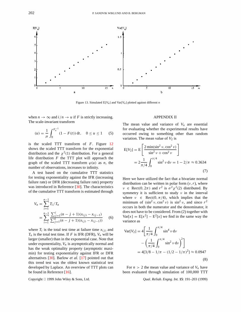
Figure 13. Simulated E[Vn] and Var[Vn] plotted against differentn

whenn → ∞ andi/n → u if F is strictly increasing.The scale-invariant transform

(u) = 1

µ

∫ F−1u

0(1 − F(t)) dt, 0 ≤ u ≤ 1 (5)

is the scaled TTT transform ofF . Figure 12shows the scaled TTT transform for the exponentialdistribution and theχ2(1) distribution. For a generallife distribution F the TTT plot will approach thegraph of the scaled TTT transformϕ(u) as n, thenumber of observations, increases to infinity.

A test based on the cumulative TTT statisticsfor testing exponentiality against the IFR (increasingfailure rate) or DFR (decreasing failure rate) propertywas introduced in Reference [30]. The characteristicsof the cumulative TTT transform is estimated through

Vn =n−1∑i=1

Ti/Tn

=n−1∑i=1

∑ij=1(n − j + 1)(x( j ) − x( j−1)∑nj=1(n − j + 1)(x( j ) − x( j−1))

(6)

whereTi is the total test time at failure timex( j ) andTn is the total test time. IfF is IFR (DFR),Vn will belarger (smaller) than in the exponential case. Note thatunder exponentiality,Vn is asymptotically normal andhas the weak optimality property (asymptotic maxi-min) for testing exponentiality against IFR or DFRalternatives [30]. Barlow et al. [17] pointed out thatthis trend test was the oldest known statistical testdeveloped by Laplace. An overview of TTT plots canbe found in Reference [16].

APPENDIX II

The mean value and variance ofVn are essentialfor evaluating whether the experimental results haveoccurred owing to something other than randomvariation. The mean value ofV2 is

E[V2] = E

[2 min(sin2 ν, cos2 ν)

sin2 ν + cos2 ν

]

= 21

π/4

∫ π/4

0sin2 ν dν = 1 − 2/π ≈ 0.3634

(7)

Here we have utilized the fact that a bivariate normaldistribution can be written in polar form (ν, r ), whereν ∈ Rect(0, 2π) and r2 is σ 2χ2(2) distributed. Bysymmetry it is sufficient to studyν in the intervalwhere ν ∈ Rect(0, π/4), which implies that theminimum of (sin2 ν, cos2 ν) is sin2 ν, and sincer2

occurs in both the numerator and the denominator, itdoes not have to be considered. From (2) together withVar[x] = E[x2] − E2[x] we find in the same way thevariance as

Var[V2] = 4

[1

π/4

∫ π/4

0sin4 ν dν

−(

1

π/4

∫ π/4

0sin2 ν dν

)2]= 4[3/8 − 1/π − (1/2 − 1/π)2] ≈ 0.0947

(8)

For n > 2 the mean value and variance ofVn havebeen evaluated through simulation of 100,000 TTT



plots for n = 2, . . . , 15. The simulations indicatestrongly that both the mean value and the varianceof the cumulative TTT transform are linear inn.Simulations performed for largern also support theassumption. The mean value of the cumulative TTTstatistic can be estimated through the formula

E[Vn] ≈ 0.3634+ 0.3634(n − 2) for n > 2 (9)

The variance of the cumulative TTT statistic can beestimated through the formula

Var[Vn] ≈ 0.0947+ 0.0993(n − 2) for n > 2(10)

Figure 13 presents E[Vn] and Var[Vn] plottedagainstn, wheren is limited to 15 for the sake ofclarity in the illustrations.

Further research is in progress to understand anddevelop the relationship for the mean value and thevariance ofVn for n > 2.

REFERENCES

1. S. Blake, R. G. Launsby and D. L. Weese, ‘Experimentaldesign meets the realities of the 1990s’,Qual. Prog.,(October), 99–101 (1994).

2. R. Koselka, ‘The new mantra: MVT’,Forbes, (11), 114–118(1996).

3. C. Daniel, ‘Use of half-normal plot in interpreting factorialtwo-level experiments’,Technometrics, 1(4), 311–341 (1959).

4. C. Daniel,Applications of Statistics to Industrial Experimen-tation, Wiley, New York, 1976.

5. G. E. P. Box and R. D. Meyer, ‘An analysis for unreplicatedfractional factorials’,Technometrics, 28(1), 11–18 (1986).

6. D. T. Voss, ‘Generalized modulus-ratio tests for analysis offactorial designs with zero degrees of freedom for error’,Commun. Statist.—Theory Meth., 17, 3345–3359 (1988).

7. H. C. Benski, ‘Use of a normality test to identify significanteffects in factorial designs’,J. Qual. Technol., 21(3), 174–178(1989).

8. R. V. Lenth, ‘Quick and easy analysis of unreplicatedfactorials’,Technometrics, 31(4), 469–473 (1989).

9. K. N. Berk and R. R. Picard, ‘Significance tests for saturatedorthogonal arrays’,J. Qual. Technol., 23, 79–89 (1991).

10. N. D. Le and R. H. Zamar, ‘A global test for effects in 2k

factorial design without replicates’,J. Statist. Comput. Simul.,41, 41–54 (1992).

11. F. Dong, ‘On the identification of active contrasts inunreplicated fractional factorials’,Statist. Sinica, 3, 209–217(1993).

12. H. Schneider, W. J. Kasperski and L. Weissfeld, ‘Findingsignificant effects for unreplicated fractional factorials usingthe n smallest contrasts’,J. Qual. Technol., 25(1), 18–27(1993).

13. J. H. Venter and S. J. Steel, ‘A hypothesis-testing approachtoward identifying active contrasts’,Technometrics, 38(2),161–169 (1996).

14. R. E. Barlow and R. Campo, ‘Reliability and fault treeanalysis’, in R. E. Barlow, J. Fussell and N. D. Singpurwalla(eds),Total Time on Test Processes and Applications to FailureData Analysis, SIAM, Philadelphia, PA, 1975, pp. 451–491.

15. B. Bergman and B. Klefsjö, ‘The total time on test conceptand its use in reliability theory’,Oper. Res., 32(3), 596–606(1984).

16. B. Bergman and B. Klefsjö, ‘Total time on test transform’,Kotz–Johnson Encyclopedia of Statistical Sciences, Vol. 9,Wiley, New York, 1988, pp. 297–300.

17. R. E. Barlow, D. J. Bartholomew and J. M. Bremner,Statistical Inference under Order Restrictions, Wiley, NewYork, 1972.

18. R. E. Barlow, ‘Geometry of the total time on test transform’,Naval Res. Logist. Q., 26, 393–402 (1979).

19. B. Bergman, F. Ekdahl and P. Sandvik Wiklund, ‘Acomparison of selection procedures for finding active contrastsin unreplicated fractional factorials’,Proc. 2nd World Conf. ofIASC, Pasadena, CA, 1997, pp. 573–582.

20. T. Klemets and T. Lithner,Industrial Design of Experiments—13 Case Studies from Swedish Industry, Studentlitteratur,Lund, 1994 (in Swedish).

21. D. S. Moore, ‘An elementary proof of asymptotic normalityof linear functions of order statistics’,Ann. Math. Statist., 39,263–265 (1968).

22. A. Birnbaum, ‘On the analysis of factorial experimentswithout replication’,Technometrics, 1(4), 343–357 (1959).

23. D. A. Zahn, ‘An empirical study of the half-normal plot’,Technometrics, 17(2), 201–211 (1975).

24. P. D. Haaland and M. A. O’Connell, ‘Inference for effect-saturated fractional factorials’,Technometrics, 37(1), 82–93(1995).

25. G. Taguchi and Y. Wu,Introduction to Off-line QualityControl, Central Japan Quality Control Association, Nagoya,1980.

26. G. E. P. Box, W. G. Hunter and J. S. Hunter,Statistics forExperimenters, Wiley, New York, 1978.

27. O. L. Davies, The Design and Analysis of IndustrialExperiments, Oliver and Boyd, London, 1994.

28. C. Hellstrand, ‘The necessity of modern quality improvementand some experiences with its implementation in themanufacture of rolling bearings’,Philos. Trans. R. Soc., 327,529–537 (1989).

29. B. Bergman, ‘On reliability theory and its applications’,Scand. J. Statist., 12(1), 1–41 (1985).

30. R. E. Barlow and K. Doksum, ‘Isotonic tests for convexorderings’, Proc. 6th Berkeley Symp. on MathematicalStatistics and Probability, Berkeley, CA, 1972. pp. 293–323.

Authors’ biographies:

Pia Sandvik Wiklund has been Assistant Professor inQuality Technology at Lule˚a University of Technologysince 1997. She received her PhD in quality engineeringfrom Linkoping University and holds an MSc degree inmechanical engineering, also from Linköping University.She was a member of the Design of Experiments andRobust Design Engineering Group in the Division of QualityTechnology and Management between 1989 and 1996.

Bo Bergman has been Professor in Quality Technologyand Management at Linköping University since 1983. Hehad 15 years of industrial experience in the fields ofreliability engineering, quality methodology and statisticalconsulting before joining the university. He received hisPhD in mathematical statistics from Lund University whileemployed at the Aerospace Division of Saab-Scania Inc. AtLinkoping University he is leading a number of researchgroups in Quality Technology and Management. He hasauthored or co-authored seven books and more than 50scientific papers.


Documents

Finding active factors from unreplicated fractional factorials utilizing the total time on test (TTT) technique