WP/07/177

Financing of Global Imbalances

W. Christopher Walker and

Maria Teresa Punzi

© 2007 International Monetary Fund WP/07/177 IMF Working Paper Monetary and Capital Markets

Financing of Global Imbalances

Prepared by W. Christopher Walker and Maria Teresa Punzi1

Authorized for distribution by Peter Dattels

July 2007

Abstract

This Working Paper should not be reported as representing the views of the IMF. The views expressed in this Working Paper are those of the author(s) and do not necessarily represent those of the IMF or IMF policy. Working Papers describe research in progress by the author(s) and are published to elicit comments and to further debate.

To assess the conditions for the financing of the U.S. current account, this paper analyzes the determinants of bond flows into the United States, using a data set constructed for the period 1994-2006 from U.S. Treasury International Capital Flow (TIC) statistics. Panel vector autoregression and instrumental variables approaches are used to estimate the impact of changes in interest rate differentials and other fundamentals on capital flows into the U.S. The paper finds evidence for an impact from interest rate differentials to bond inflows that has increased over time, consistent with a theoretical model of declining home bias. JEL Classification Numbers: F32, G15 Keywords: home bias, panel VAR, U.S. bond inflows Author’s E-Mail Address: cwalker@imf.org, punzi@bc.edu 1 IMF and Boston College, respectively. The authors wish to thank Ravi Balakrishnan, Stephen Bond, Elie Canetti, Peter Dattels, Hali Edison, Gian Maria Milesi-Ferretti, and Martin Muhleisen for valuable discussions. They also wish to thank Inessa Love for the use of her panel VAR program.

Contents Page I. Introduction ...........................................................................................................................3 II. Literature Survey.................................................................................................................. 4 A. Home Bias.................................................................................................................4 B. Determinants of Equity Flows...................................................................................5 C. Fixed Income Flows and Bond Yields......................................................................5 III. Theoretical Model................................................................................................................6 IV. Data......................................................................................................................................8 V. Empirical Estimation..........................................................................................................11 VI. Identification Issues...........................................................................................................13 VII. Panel Instrumental Variable Estimates.............................................................................13 VIII. Panel VARs and Impulse Response Functions...............................................................16 IX. Conclusion.........................................................................................................................18 Figures 1. Sources of Financing for the U.S. Current Account Deficit..........................................4 2. Japan – Holdings of Long-Term U.S. Bond Debt.........................................................9 3. Impulse Response Functions........................................................................................18 Tables 1. Summary Statistics for Period 1 Data (1/95-12/01).....................................................11 2. Summary Statistics for Period 2 Data (1/02-4/06).......................................................11 3. Correlations Between Interest Spreads and Exchange Rate Expectations...................12 4. Pooled Two-Stage Least Squares Regressions............................................................14 5. Fixed Effects Two-Stage Least Squares Regressions..................................................15 6. “Partial Fixed Effects” 2SLS Regressions...................................................................16 7. Correlation Coefficients and Std Dev of Residuals from Pd 2 VAR...........................17 Appendix Panel Estimates Without Instrumental Variables....................................................................20

2

3

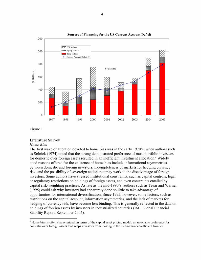
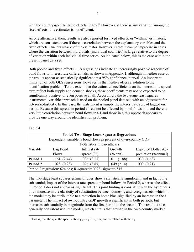
Introduction Since 1994, international capital markets have grown severalfold, with an increase in cross-border capital flows of more than 500 percent.2 Over the same period, the incidence of observed home bias, as indicated by the share of foreign assets in the portfolios of investors from a given country, has diminished in most developed countries and for most classes of investors. This increased degree of financial integration appears to be due to several factors, including the rapid development of international trade, some reduction in the use of capital controls, the development of sophisticated financial instruments for handling currency and other risks, and, in some cases, better marketing of financial products constructed from foreign assets. It has become almost standard practice to draw a close connection between financial integration and the development of large current account imbalances, notably in the United States. Greater international financial integration raises the prospect of easier financing for a country running a fiscal or current account deficit. At the same time, it may be expected that capital flows would become more responsive to changes in relative conditions – including relative interest rates – across borders. Accordingly, in a world of large current account imbalances, changes in relative interest rates or other conditions that might once have had only a muted impact internationally, could lead to sharp changes in capital flows or exchange rates. The present paper focuses on bond flows, which have been the dominant source of private sector funding for the US current account deficit (Figure 1).3 It begins with a brief review of the extensive literature in the field, and the presentation of a simple two-country theoretical model – based largely on the recent dynamic model of Blanchard, Giavazzi, and Sa (2005) – in order to establish which factors should influence bond flows. The empirical part of the paper concentrates on estimating the impact on bond purchases of expectations for probable returns on an investment in foreign bonds. Successive time spans are examined to see if the impact has increased over time. To exploit the cross-sectional structure of the data and to correct for the endogeneity of key independent variables – notably the spread differential between interest rates in the home market and those in the US – both panel VAR and panel instrument variables approaches are used. The conclusion summarizes these results, interpreting them in terms of the theoretical model, and more broadly.

2 IMF Balance of Payment Statistics, 2006. Percentage increase in gross financial account outflows, all countries, from 1994 to 2005.

3 For example, net bond (including Treasuries, agencies, and corporates) purchases by foreigners accounted for more than 88% of portfolio inflows in the 12 months through October 2006, and more than 100% of the current account deficit during that period.

4

Sources of Financing for the US Current Account Deficit

0

200

400

600

800

1000

1200

1997 1998 1999 2000 2001 2002 2003 2004 2005

$ B

illio

n

FDI InflowsEquity InflowsBond InflowsCurrent Account Deficit (-)

Source: IMF

Figure 1

Literature Survey Home Bias The first wave of attention devoted to home bias was in the early 1970’s, when authors such as Solnick (1974) noted that the strong demonstrated preference of most portfolio investors for domestic over foreign assets resulted in an inefficient investment allocation.4 Widely cited reasons offered for the existence of home bias include informational asymmetries between domestic and foreign investors, incompleteness of markets for hedging currency risk, and the possibility of sovereign action that may work to the disadvantage of foreign investors. Some authors have stressed institutional constraints, such as capital controls, legal or regulatory restrictions on holdings of foreign assets, and even constraints entailed by capital risk-weighting practices. As late as the mid-1990’s, authors such as Tesar and Warner (1995) could ask why investors had apparently done so little to take advantage of opportunities for international diversification. Since 1995, however, some factors, such as restrictions on the capital account, information asymmetries, and the lack of markets for hedging of currency risk, have become less binding. This is generally reflected in the data on holdings of foreign assets by investors in industrialized countries (IMF Global Financial Stability Report, September 2005). 4 Home bias is often characterized, in terms of the capital asset pricing model, as an ex ante preference for domestic over foreign assets that keeps investors from moving to the mean-variance-efficient frontier.

5

Determinants of Equity Flows Much of the analytical work devoted to quantifying the determinants of cross-border capital flows has focused on equity flows. In a recent paper, Portes and Rey (2005) explore a “gravity” model of cross-border equity flows using a panel data set on bilateral flows among 14 industrialized economies. They find that both geographical distance, and a set of proxy variables for information asymmetries, explain a substantial portion of the variation in the equity portfolios of investors in individual countries. Edison and Warnock (2006) concentrate on the effects of capital account liberalization on equity inflows to emerging markets using a panel data set constructed from the TIC. Over the period of the study, which is primarily the 1990’s, they find a strong short-term impact of liberalization measures on equity inflows, and a more attenuated long-term effect. Fixed Income Flows and Bond Yields There is a substantial recent literature discussing the impact of foreign capital flows on the dollar and on US bond yields. Both recent US Federal Reserve Chairmen, Alan Greenspan and Ben Bernanke, have provided detailed accounts of the role of foreign inflows in financing US fiscal and current account deficits. Greenspan (2005) notes a secular reduction in home bias, both in the US and elsewhere, and indicates that this shift has made it possible for individual countries to run large deficits for sustained periods. He also concludes, however, that the drop in home bias may have also increased the sensitivity of inflows to interest rate differentials, exchange rate expectations, and other factors. Bernanke (2005) focuses on a “global savings glut” that, he argues, has lowered long-term real interest rates around the world, and increased the US current account deficit. In a recent series of theoretical contributions, Dooley, Folkerts-Landau, and Garber (2003) argue that low Treasury yields and the accompanying support for the dollar stemming from cross-border inflows to the Treasury market reflect a tacit “Bretton Woods II” policy equilibrium in which net borrowers accept currency strength in return for financing of their deficits, in the form of foreign official bond purchases. However, authors such as Lane and Milesi-Ferretti (2005) have argued that such an arrangement could not represent a sustainable long-term equilibrium. Related studies include several others devoted to explaining and quantifying the “conundrum” of low long-term US Treasury yields described by both Greenspan and Bernanke. Using TIC data on official purchases of Treasuries, Frey and Moec (2005) find that long-term US Treasury yields would have been up to 115 bps higher in 2004 had it not been for foreign central bank buying. Warnock and Warnock (2005) estimate the impact of overall foreign inflows on bond yields using OLS regressions on aggregate, adjusted, TIC data. They find a total impact from foreign inflows on US long-term bond yields of 150 basis points at the time of the study. Testing for a causal connection running from returns to bond flows, Lane and Milesi-Ferretti (2005) do not find evidence of a positive correlation between lagged returns and inflows to the bond market, but do find such a correlation in the case of equities.

6

Theoretical Model A simple two-country theoretical model is based on that of Blanchard, Giavazzi, and Sa (2005). Following Blanchard et al, national wealth is WU=XU-F for the United States (U), where XU is the value of the US asset market and F is the net debt of the US. Similarly, for the other country, simply designated V, WV/ε = XV/ε+ F, where ε is the exchange rate expressed as the number of units of V currency per dollar. The share of WU in domestic assets is σU(R,s), where :

t

tt

V

U

rr

Rεε 1

11 +

++

=

As implied by the equation, R is the uncovered interest parity ratio, while s is a parameter expressing the degree of home bias on the part of US investors. If s=0, US investors hold only US assets – a higher s denotes lower home bias, and entails a greater share of non-US assets held by US residents. Similarly, for the foreign country, the share of national wealth WV held in own-market assets is σV(R,t). An alternative and equivalent characterization, which will be useful for the analysis, is that the share of V’s national wealth held in US assets is η(R,t) such that η(R,t) = 1-σV(R,t). η(.) is increasing in both R and t. A value of R above 1 means the interest rate spread favors US assets. The t parameter denotes the degree of home bias of country V, such that if t=0, country V investors hold only V assets. It will be useful to attach a specific functional form to the η(R,t) function. A convenient form is:

11

11

1),( −−

−−

−+−

=eee

eeetR Rt

Rt

η

where t varies from 0 to 1, and R > 0. It is also assumed that 0 < t < 1, and that R and t are such that 0 < η < ½ . Conversely, σV, the share of country V assets held by domestic V investors, varies from one to one-half. For purposes of this simplified model, it is assumed that US investors hold only US assets and that, accordingly, s = 0 and σU(R,s) = 1.5 It follows that, for foreign investors, XV = σV(R,t)(XV + Fε). Substituting η=1-σV, and rearranging terms:

VXF ⎥⎦

⎤⎢⎣

⎡−

=η

ηε1

Taking the time derivative:

5 In the real world, this assumption is approximately true for bonds, and clearly not true with regard to equities. Because we are focusing on the bond case, we maintain it here.

7

}VV XXF

•••

Φ+Φ=ε where Φ= η/(1-η) = e-1eRt-e-1 Equivalently:

Equation 1 }

( ) VRt

VRt XtRRteeXeeeF ⎟

⎠⎞

⎜⎝⎛ ++−=

••−

•−−

•111ε

Dividing through by XV (to be proxied by GDP), and rearranging, yields:

Equation 2

}

V

VRt

V

VRt

V XXetRRtee

XXee

XF

•

−••

−

•

−

•

−⎟⎠⎞

⎜⎝⎛ ++= 111ε

This equation will be used as a framework for the empirical specification of bond flows. Given that t, and R, and e-1eRt are all positive, and that e-1eRt > e-1,it follows that bond flows are a positive function of GDP growth, of R

．, and of t

． (that is, of reductions in home bias). To

determine the impact of a higher uncovered interest parity ratio R on bond flows, take the derivative of Equation 2 with respect to R:

Equation 3

}

⎟⎟⎟

⎠

⎞

⎜⎜⎜

⎝

⎛+++=

••••

−

•

tRttRXXtee

dRXFd

tV

VRtV 21

ε

Assuming that both t

． and X

． are either positive or zero (i.e., that home bias is either staying

the same or falling, and the economy is stagnant or growing), then a higher R leads, in general, to higher bond flows. The only exception would be in a case where R

． is very

negative, in the sense that -R．/R > t

．/t + (1/Rt)( t

．/t + X

．/X). Not only does the model entail that

a higher R will induce higher bond flows in general, but it also implies that a reduction in home bias should increase the sensitivity of bond flows to the uncovered interest parity ratio. This is shown by taking the derivative of Equation 3 with respect to t, which yields a value that is positive under similar conditions to those applying to Equation 3.

8

Equation 4

}

⎟⎟⎟

⎠

⎞

⎜⎜⎜

⎝

⎛+++

⎟⎟⎟

⎠

⎞

⎜⎜⎜

⎝

⎛+++=

•••

−•••

•

−

•

RttRXX

eetRttRXXte

dRdtXF

V

VRt

V

VRtV td

2Re 121

2 ε

These equations represent a special case of the Blanchard model, and are therefore consistent with that model. One important implication of the model is that a shift in the home bias parameter affects the exchange rate ε in opposite ways in the short and the long term. Over the short term, an increase in t (and therefore a reduction in country V home bias) will cause the dollar to appreciate as it increases outflows to the US. However, in the long-run steady state the dollar is weaker than if t had not risen, because the buildup of F has been larger than it would have been otherwise, and the weaker dollar is required to generate the trade surplus that the US needs to service that larger debt F. Data Panel data on capital flows are obtained from the US Treasury International Capital Flows dataset over the period 1994-2006. The data show flows of bonds and equities between the United States and other jurisdictions, on a bilateral basis. An important limitation of the data is that, while they show the country of residence of the entity through which the assets are initially purchased, they do not necessarily reveal the source of final demand for the assets. For example, if a Dutch pension fund purchases a U.S. Treasury bond through a British bank, the transaction would be recorded in the TIC as a portfolio bond inflow from the UK to the US, rather than from the Netherlands. In order to minimize this “custodial” bias, which results the overstatement of flows to and from financial centers such as the UK, the Cayman Islands, and Singapore, the data are adjusted to match less frequent, but more accurate, custodial data on stocks of foreign holdings of US assets.6 Such data have been published at irregular intervals, but most recently have been made available on an annual basis. Before making the corrections for the less frequent custodial data, however, it is necessary first to take account of the impact of transactions, and of changes in prices and exchange rates, on measured holdings levels in the monthly data. This entails calculating the increase or loss in value with respect to the principal over time of some securities, like asset-backed and zero-coupon securities. After Warnock (2005), the following equation is used to adjust for price changes and for gross purchases and sales:

itititittiti TGSGPNPrAA )()1( ,,,1,, +−++= − 6 The data cover all flows to the United States, and so incorporate both private and public flows, which, as suggested by the example, are often difficult to distinguish in practice. Admittedly, bond purchases by public entities may be insulated to some extent from market forces. However, public entities, like private ones, are often sensitive to implicit interest rate differentials, in many cases weighing the cost of issuing domestic debt against the yield earned on foreign reserves

9

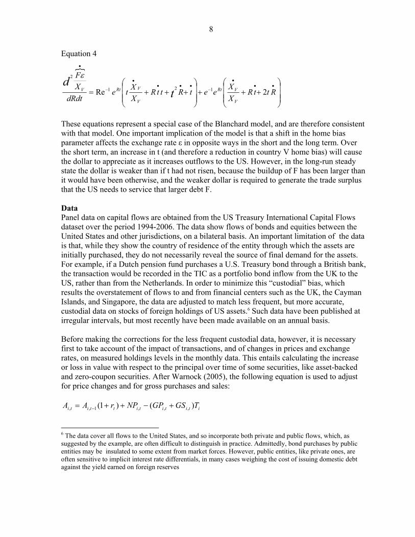
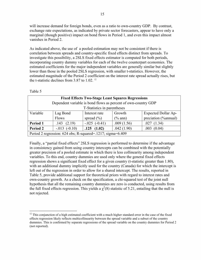
where Ai,t = holdings of U.S. securities by country i’s residents at the end of month t (includes Treasuries, corporates, and agencies), rt = return index for revaluing holdings, NPi,t = net purchases of U.S. securities by country i’s residents during month t, GPi,t = gross purchases of U.S. securities by country i’s residents during month t, GSi,t = gross sales of U.S. securities by country i’s residents during month t, and Ti is an adjustment factor for transaction costs. Transactions costs are set at 5 basis points on U.S. Treasury debt, 10 basis points on U.S. agency debt, and 25 basis points on U.S. corporate debt. Even after adjusting for transaction bias, the resulting estimates differ, sometimes consider-ably, from what the less frequent custodial survey indicates, as would be expected in the presence of custodial bias. Therefore an interpolation method is used to smooth the resulting data, multiplying the indicated flows by a calculated ratio such that cumulative flows at the end of the period match the difference between the initial and terminal stocks in each interval in the custodial survey. Figure 2 shows the effects of adjusting the data in this way:

Japan - Holdings of Long-Term US Bond Debt

0

100

200

300

400

500

600

700

800

900

1000

Jun-94

Dec-94

Jun-95

Dec-95

Jun-96

Dec-96

Jun-97

Dec-97

Jun-98

Dec-98

Jun-99

Dec-99

Jun-00

Dec-00

Jun-01

Dec-01

Jun-02

Dec-02

Jun-03

Dec-03

Jun-04

Dec-04

Jun-05

Dec-05

Jun-06

$US

Bill

ions

Estimated Bonds Adjusted Bonds

Sources: TIC, staff calculations

Figure 2

Data on local market bond yields and currency rates are provided by Bloomberg. Macroeconomic data, including GDP growth data, are from the Fund’s International Financial Statistics database. The interest rates chosen for determining spreads are long-term

10

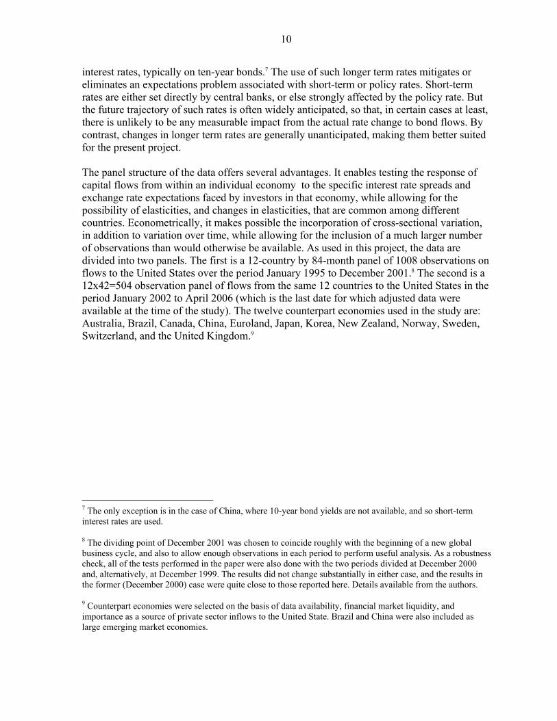
interest rates, typically on ten-year bonds.7 The use of such longer term rates mitigates or eliminates an expectations problem associated with short-term or policy rates. Short-term rates are either set directly by central banks, or else strongly affected by the policy rate. But the future trajectory of such rates is often widely anticipated, so that, in certain cases at least, there is unlikely to be any measurable impact from the actual rate change to bond flows. By contrast, changes in longer term rates are generally unanticipated, making them better suited for the present project. The panel structure of the data offers several advantages. It enables testing the response of capital flows from within an individual economy to the specific interest rate spreads and exchange rate expectations faced by investors in that economy, while allowing for the possibility of elasticities, and changes in elasticities, that are common among different countries. Econometrically, it makes possible the incorporation of cross-sectional variation, in addition to variation over time, while allowing for the inclusion of a much larger number of observations than would otherwise be available. As used in this project, the data are divided into two panels. The first is a 12-country by 84-month panel of 1008 observations on flows to the United States over the period January 1995 to December 2001.8 The second is a 12x42=504 observation panel of flows from the same 12 countries to the United States in the period January 2002 to April 2006 (which is the last date for which adjusted data were available at the time of the study). The twelve counterpart economies used in the study are: Australia, Brazil, Canada, China, Euroland, Japan, Korea, New Zealand, Norway, Sweden, Switzerland, and the United Kingdom.9

7 The only exception is in the case of China, where 10-year bond yields are not available, and so short-term interest rates are used.

8 The dividing point of December 2001 was chosen to coincide roughly with the beginning of a new global business cycle, and also to allow enough observations in each period to perform useful analysis. As a robustness check, all of the tests performed in the paper were also done with the two periods divided at December 2000 and, alternatively, at December 1999. The results did not change substantially in either case, and the results in the former (December 2000) case were quite close to those reported here. Details available from the authors.

9 Counterpart economies were selected on the basis of data availability, financial market liquidity, and importance as a source of private sector inflows to the United State. Brazil and China were also included as large emerging market economies.

11

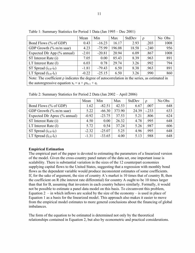
Table 1: Summary Statistics for Period 1 Data (Jan 1995 – Dec 2001)

Mean Min Max StdDev ρ No Obs Bond Flows (% of GDP) 0.43 -16.23 16.17 2.93 .203 1008GDP Growth (% m/m saar) 4.23 -75.99 196.08 18.58 -.240 956Expected Dlr App (% annual) -2.01 -20.81 20.94 6.09 .867 1008ST Interest Rate (i) 7.05 0.00 85.43 8.39 .963 891LT Interest Rate (l) 6.03 0.78 29.74 3.26 .992 794ST Spread (iUS-iF) -1.81 -79.43 6.50 8.38 .963 891LT Spread (lUS-lF) -0.22 -25.15 6.50 3.26 .990 860Note: The coefficient ρ indicates the degree of autocorrelation in the series, as estimated in the autoregressive equation xt = a + ρxt-1 + et

Table 2: Summary Statistics for Period 2 Data (Jan 2002 – April 2006)

Mean Min Max StdDev ρ No Obs Bond Flows (% of GDP) 1.62 -82.51 42.53 6.67 .007 648GDP Growth (% m/m saar) 5.22 -66.30 373.90 24.39 -.233 633Expected Dlr Aprec (% annual) -0.92 -23.75 37.53 5.21 .806 624ST Interest Rate (i) 4.50 0.00 26.32 4.78 .995 648LT Interest Rate (l) 5.72 0.54 37.24 5.26 .987 606ST Spread (iUS-iF) -2.32 -25.07 5.25 4.96 .995 648LT Spread (lUS-lF) -1.31 -33.65 4.00 5.13 .988 648

Empirical Estimation The empirical part of the paper is devoted to estimating the parameters of a linearized version of the model. Given the cross-country panel nature of the data set, one important issue is scalability. There is substantial variation in the sizes of the 12 counterpart economies supplying capital flows to the United States, suggesting that a regression with monthly bond flows as the dependent variable would produce inconsistent estimates of some coefficients. If, for the sake of argument, the size of country A’s market is 10 times that of country B, then the coefficient on R (the interest rate differential) for country A ought to be 10 times larger than that for B, assuming that investors in each country behave similarly. Formally, it would not be possible to estimate a panel data model on this basis. To circumvent this problem, Equation 2 – in which inflows are scaled by the size of the economy – is used in place of Equation 1 as a basis for the linearized model. This approach also makes it easier to move from the empirical model estimates to more general conclusions about the financing of global imbalances. The form of the equation to be estimated is determined not only by the theoretical relationships contained in Equation 2, but also by econometric and practical considerations.

12

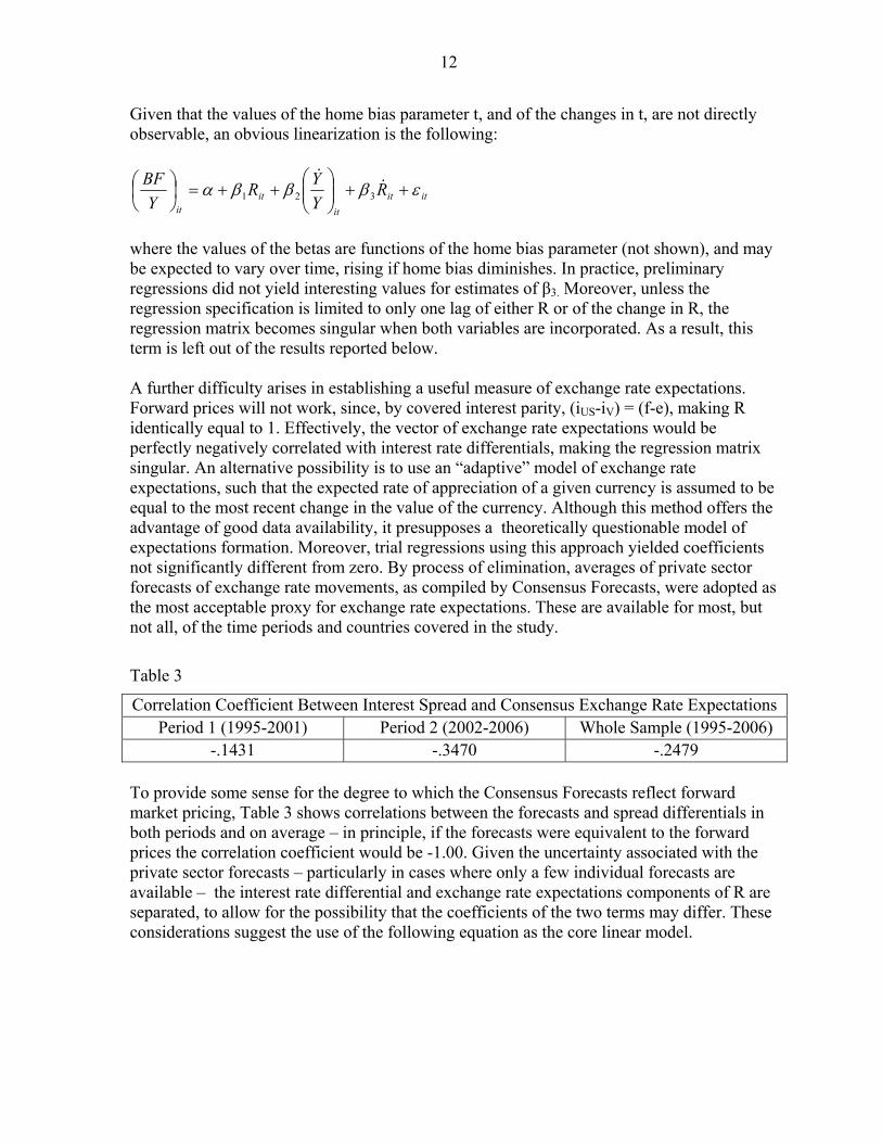
Given that the values of the home bias parameter t, and of the changes in t, are not directly observable, an obvious linearization is the following:

ititit

itit

RYYR

YBF εβββα ++⎟⎟

⎠

⎞⎜⎜⎝

⎛++=⎟

⎠⎞

⎜⎝⎛ &

&321

where the values of the betas are functions of the home bias parameter (not shown), and may be expected to vary over time, rising if home bias diminishes. In practice, preliminary regressions did not yield interesting values for estimates of β3. Moreover, unless the regression specification is limited to only one lag of either R or of the change in R, the regression matrix becomes singular when both variables are incorporated. As a result, this term is left out of the results reported below. A further difficulty arises in establishing a useful measure of exchange rate expectations. Forward prices will not work, since, by covered interest parity, (iUS-iV) = (f-e), making R identically equal to 1. Effectively, the vector of exchange rate expectations would be perfectly negatively correlated with interest rate differentials, making the regression matrix singular. An alternative possibility is to use an “adaptive” model of exchange rate expectations, such that the expected rate of appreciation of a given currency is assumed to be equal to the most recent change in the value of the currency. Although this method offers the advantage of good data availability, it presupposes a theoretically questionable model of expectations formation. Moreover, trial regressions using this approach yielded coefficients not significantly different from zero. By process of elimination, averages of private sector forecasts of exchange rate movements, as compiled by Consensus Forecasts, were adopted as the most acceptable proxy for exchange rate expectations. These are available for most, but not all, of the time periods and countries covered in the study.

Table 3

Correlation Coefficient Between Interest Spread and Consensus Exchange Rate Expectations Period 1 (1995-2001) Period 2 (2002-2006) Whole Sample (1995-2006)

-.1431 -.3470 -.2479 To provide some sense for the degree to which the Consensus Forecasts reflect forward market pricing, Table 3 shows correlations between the forecasts and spread differentials in both periods and on average – in principle, if the forecasts were equivalent to the forward prices the correlation coefficient would be -1.00. Given the uncertainty associated with the private sector forecasts – particularly in cases where only a few individual forecasts are available – the interest rate differential and exchange rate expectations components of R are separated, to allow for the possibility that the coefficients of the two terms may differ. These considerations suggest the use of the following equation as the core linear model.

13

Equation 5

itit

ititttiUSit Y

YeeErrY

BF εβββα +⎟⎟⎠

⎞⎜⎜⎝

⎛+−+−+=⎟

⎠⎞

⎜⎝⎛

+

&3121 )1/)(()(

Identification Issues Estimation of the parameters of Equation 5 raises standard identification issues typically associated with estimation of supply and demand elasticities. In particular, the spread variable (rUS-ri) is likely to be correlated with the error term εit, given that higher bond inflows (i.e., an increase in the quantity demanded) should be expected to lead to a lower spread (i.e., a higher price of US bonds). Two distinct approaches are used to minimize the identification problem. First, a heteroskedasticity-adjusted two-stage least squares estimator is used.10 As an alternative approach to identification, and in order to capture possible lagged impacts lasting over several periods, a panel data VAR is also estimated. Of course, one may adopt as an identifying assumption the view that while bond flows in period t may cause changes in the spread during t, the converse will not be the case – a change in the spread in period t does not lead to a change in bond flows in that period. However, given that monthly data is used, and that flows of “hot money” may respond to price changes with much less than one month’s lag, it would appear safer to not to take such a relationship as given. Accordingly, in the instrumental variables estimation, the spread variable lagged one period is used as an instrument for the same-period spread, ruling out this potential channel of causation. In the case of the panel VAR, some identifying assumption is still needed about the direction of causation of same-period shocks. That is, if the shock to spreads in period t is correlated with the shock to bond flows, then an assumption needs to be made about which of the two is the “first” shock. Here, the convention, as reflected in the preceding paragraph, is to assume that price (spread) responds more rapidly to a change in quantity demanded than the converse. This would be accommodated in the VAR framework by assuming that the initial shock is to bond flows, so that the same-period impact of a change in spreads on flows is assumed to be zero. However, the robustness of this assumption can be examined be reversing the order of the shocks to see if there is an appreciable difference in impulse response functions. Panel Instrumental Variable Estimates In working with panel data, it is standard to report results for more than one type of estimator, given that the underlying characteristics of the statistical process or processes being analyzed are not known with certainty. A pooled data estimator, which treats observations on separate countries as though they were all drawn from the same population, will be consistent as long as the explanatory variables (notably, spreads) are uncorrelated 10 In this context, Hsiao recommends the use of a model in which independent and dependent variables are all first-differenced. However, this procedure eliminates the spread levels information which, from the theoretical model, is a determinant of bond inflows.

14

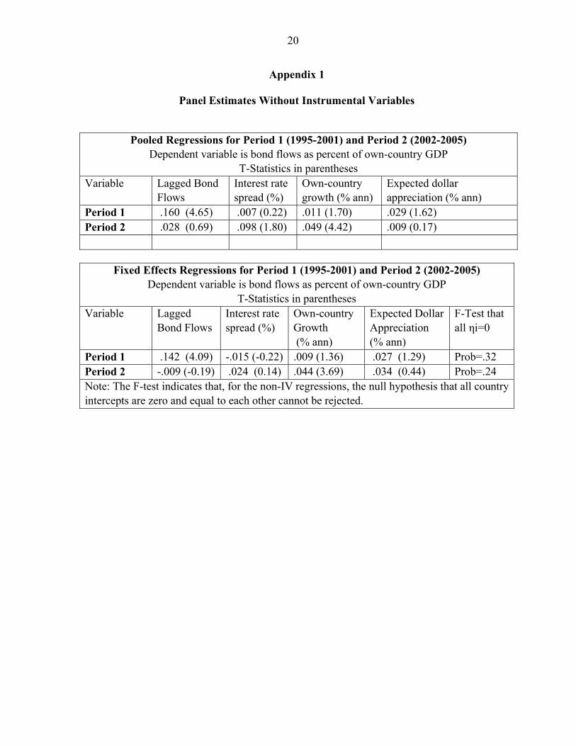
with the country-specific fixed effects, if any.11 However, if there is any variation among the fixed effects, this estimator is not efficient. As one alternative, then, results are also reported for fixed effects, or “within,” estimators, which are consistent even if there is correlation between the explanatory variables and the fixed effects. One drawback of the estimator, however, is that it can be imprecise in cases where the variation between individuals (individual countries) is large relative to the degree of variation within each individual time series. As indicated below, this is the case within the present panel data set. Both pooled and fixed effects OLS regressions indicate an increasingly positive response of bond flows to interest rate differentials, as shown in Appendix 1, although in neither case do the results appear as statistically significant at a 95% confidence interval. An important limitation of both OLS regressions, however, is that neither offers a solution to the identification problem. To the extent that the estimated coefficients on the interest rate spread term reflect both supply and demand shocks, those coefficients may not be expected to be significantly positive, or even positive at all. Accordingly the two-stage least squares instrumental variable approach is used on the pooled panel data set, with an adjustment for heteroskedasticity. In this case, the instrument is simply the interest rate spread lagged one period. Because this spread in period t-1 cannot be affected by bond flows in t, and there is very little correlation between bond flows in t-1 and those in t, this approach appears to provide one way around the identification problem.

Table 4

Pooled Two-Stage Least Squares Regressions Dependent variable is bond flows as percent of own-country GDP

T-Statistics in parentheses Variable Lag Bond

Flows Interest rate spread (%)

Growth (% ann)

Expected Dollar Ap-preciation (%annual)

Period 1 .161 (2.44) .006 (0.27) .011 (1.88) .030 (1.68) Period 2 .028 (0.23) .096 (3.87) .049 (2.14) .009 (0.21) Period 2 regression: 624 obs; R-squared=.0923; sigma=6.515 The two-stage least squares estimator does show a statistically significant, and in fact quite substantial, impact of the interest rate spread on bond inflows in Period 2, whereas the effect in Period 1 does not appear as significant. This joint finding is consistent with the hypothesis of an increase in the elasticity of substitution between domestic and foreign assets, which in the model may be attributable to a reduction in home bias, signified by an increase in the t parameter. The impact of own-country GDP growth is significant in both periods, but increases substantially in magnitude from the first period to the second. This result is also generally consistent with the model, which entails that growth in the own-country market 11 That is, that the ηi in the specification yit = xitβ + ηi + υit are correlated with the xit.

15

will increase demand for foreign bonds, even as a ratio to own-country GDP. By contrast, exchange rate expectations, as indicated by private sector forecasters, appear to have only a marginal (though positive) impact on bond flows in Period 1, and even this impact almost vanishes in Period 2. As indicated above, the use of a pooled estimation may not be consistent if there is correlation between spreads and country-specific fixed effects distinct from spreads. To investigate this possibility, a 2SLS fixed effects estimator is computed for both periods, incorporating country dummy variables for each of the twelve counterpart economies. The estimated coefficients for the major independent variables are generally similar but slightly lower than those in the pooled 2SLS regression, with smaller t-statistics. However, the estimated magnitude of the Period 2 coefficient on the interest rate spread actually rises, but the t-statistic declines from 3.87 to 1.02. 12

Table 5

Fixed Effects Two-Stage Least Squares Regressions Dependent variable is bond flows as percent of own-country GDP

T-Statistics in parentheses Variable Lag Bond

Flows Interest rate spread (%)

Growth (% ann)

Expected Dollar Ap-preciation (%annual)

Period 1 .143 (2.19) -.025 (-0.41) .009 (1.56) .027 (1.34) Period 2 -.013 (-0.10) .125 (1.02) .042 (1.90) .003 (0.04) Period 2 regression: 624 obs; R-squared=.1217; sigma=6.409 Finally, a “partial fixed effects” 2SLS regression is performed to determine if the advantage in consistency gained from using country intercepts can be combined with the potentially greater precision of a pooled estimate in which there is less collinearity among independent variables. To this end, country dummies are used only where the general fixed effects regression shows a significant fixed effect for a given country (t-statistic greater than 1.80), with an additional dummy implicitly used for the country (Canada) for which the intercept is left out of the regression in order to allow for a shared intercept. The results, reported in Table 5, provide additional support for theoretical priors with regard to interest rates and own-country growth. As a check on the specification, a chi-squared test of the joint null hypothesis that all the remaining country dummies are zero is conducted, using results from the full fixed effects regression. This yields a χ2(8) statistic of 5.21, entailing that the null is not rejected.

12 This conjunction of a high estimated coefficient with a much higher standard error in the case of the fixed effects regression likely reflects multicollinearity between the spread variable and a subset of the country dummies. This is confirmed by separate regressions of the spread variable on the country dummies for Period 2 (not reported).

16

Table 6

“Partial Fixed Effects” Two-Stage Least Squares Regressions Dependent variable is bond flows as percent of own-country GDP. Country dummies used for Canada, China, Korea, and Switzerland.

T-Statistics in parentheses Variable Lag Bond Flows Interest rate

spread (%) Growth (% ann)

Expected Dollar Apprec (%ann)

Period 2 -.006 (-0.05) .066 (2.72) .043 (2.04) .017 (0.42) Chi-squared test of maintained hypothesis that all but three country intercepts (China, Korea, Switzerland) are zero; Prob > chi2=0.7346, entailing that the null hypothesis is not rejected. On balance, the results presented in Table 5 accord well with the theoretical priors, lending support to the notion that the average level of home bias declined from Period 1 to Period 2. Equivalently, demand for foreign bonds increased relative to domestic bonds, and the elasticity of substitution between the two types of assets rose. The coefficient on exchange rate expectations does not appear as significant in either period for either of the measures of exchange rate expectations employed (adaptive or consensus). This may reflect inadequacies in the available expectations measures. An alternative view, consistent with these results, is that investors may tend to regard short-term exchange rate movements as a random walk with no drift, contrary to the implications of the uncovered interest parity hypothesis. Panel VARs and Impulse Response Functions A different approach to the estimation problem is provided by panel vector autoregressions. The use of vector autoregressions in a panel data setting is still relatively new, and there are some variations in the methods used by different researchers. The panel VARs presented here are computed from a program written by Inessa Love, and based on the following model incorporating fixed effects: 13

itiititit efYYY ++Γ+Γ+Γ= −− 22110 where the Ys are vectors of dependent variables, in this case bond flows and spreads. The fixed effects fi are calculated using the Helmert procedure of forward mean-differencing. This procedure avoids the correlation between the lagged dependent variable and the fixed effects that arises from mean-differencing over the entire sample. Monte Carlo simulations are used to generate confidence intervals. The regressions are estimated with two lags of the endogenous variables. Vector autoregressions were estimated for each of the two periods (1995-2001, and 2002-2006) distinguished in the preceding sections, using two lags of each variable. All four main variables – bond flows, GDP growth, interest rate spread, and exchange rate expectations –

13 See Love, Inessa and Lea Zicchino, “Financial Development and Dynamic Investment Behavior: Evidence from Panel Vector Autoregression”

17

were treated as endogenous. Table 7 reports the matrix of correlations of residuals from each of the four estimated equations in the Period 2 VAR, along with standard deviations for the residuals from each of the four constituent equations. As suggested by the low correlation coefficient between bond flows and the spread variable, and to a lesser extent, between the expected dollar appreciation variable and bond flows, the ordering of the variables made little difference to the estimated impulse response functions. Variables were ordered as shown in the table.

Table 7

Correlation Coefficients and Std Dev of Residuals from Period 2 VAR Correlation w/

Bond Flows Correlation w/ Spread

Correlation w/ Exp Dlr App

Standard Deviation

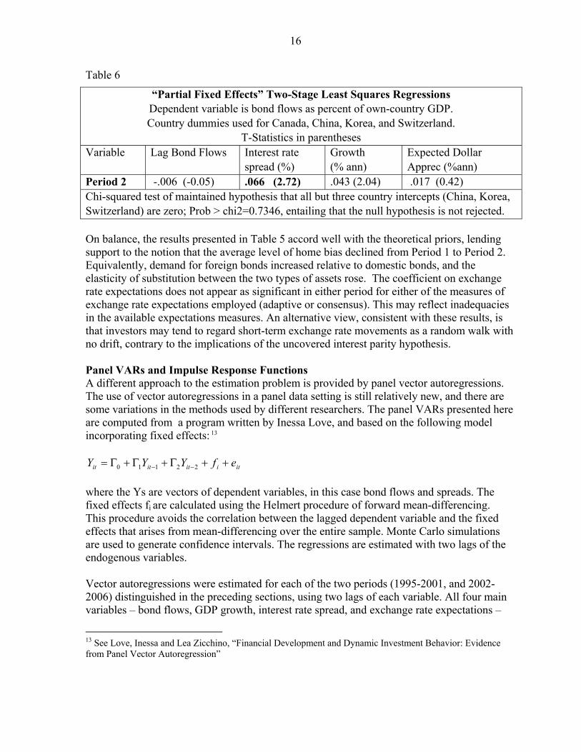
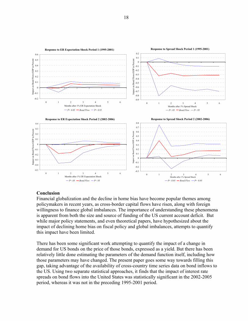
GDP Growth .1797 -.0184 .0544 22.7007 Bond Flows .0115 .0679 6.7722 Spread .3176 0.6826 Exp Dollar App 3.2630 As presented in Figure 3 below, the panel VARs show a dramatic increase in the responsiveness of bond flows to interest rate changes between Periods 1 and 2. In the former case the response is not even positive, while in the latter it is positive, statistically significant over the long run, and greater than in the two-stage least squares regression. The response to a positive spread shock in Period 2 (Figure 3) appears to be persistent, consistent with the theoretical model. The response to the exchange rate appreciation shock is significantly positive in Period 1 – as distinguished from the 2SLS results – but vanished in Period 2. Responses to GDP growth shocks (not shown) were positive but insignificant. Given the use of the bond-flow-to-GDP measure as an endogenous variable, it is possible to scale the impulse response function in the lower right corner of Figure 3 to the size of the non-US world economy. On the basis of a world economy producing approximately $44 trillion in output in 2005, of which about $12 trillion was produced in the United States, these results suggest that a 1% reduction in the interest rate spread between the United States and the rest of the world would reduce bond inflows to the US by about $53 billion over the course of a year.

18

Conclusion Financial globalization and the decline in home bias have become popular themes among policymakers in recent years, as cross-border capital flows have risen, along with foreign willingness to finance global imbalances. The importance of understanding these phenomena is apparent from both the size and source of funding of the US current account deficit. But while major policy statements, and even theoretical papers, have hypothesized about the impact of declining home bias on fiscal policy and global imbalances, attempts to quantify this impact have been limited. There has been some significant work attempting to quantify the impact of a change in demand for US bonds on the price of those bonds, expressed as a yield. But there has been relatively little done estimating the parameters of the demand function itself, including how those parameters may have changed. The present paper goes some way towards filling this gap, taking advantage of the availability of cross-country time series data on bond inflows to the US. Using two separate statistical approaches, it finds that the impact of interest rate spreads on bond flows into the United States was statistically significant in the 2002-2005 period, whereas it was not in the preceding 1995-2001 period.

Response to ER Expectation Shock Period 1 (1995-2001)

-0.2

-0.1

0

0.1

0.2

0.3

0.4

0.5

0.6

0 1 2 3 4 5 6Months after 1% ER Expectation Shock

Impa

ct o

n B

ond

Flow

s/G

DP

in P

erce

nt

P= 0.05 Bond Flow P= 0.95

Response to Spread Shock Period 1 (1995-2001)

-0.9

-0.8

-0.7

-0.6

-0.5

-0.4

-0.3

-0.2

-0.1

0

0.1

0.2

0 1 2 3 4 5 6Months after 1% Spread Shock

Impa

ct o

n B

ond

Flow

s/G

DP

in P

erce

nt

P=.05 Bond Flow P=.95

Response to ER Expectation Shock Period 2 (2002-2006)

-0.5

-0.4

-0.3

-0.2

-0.1

0

0.1

0.2

0.3

0.4

0 1 2 3 4 5 6Months after 1% ER Expectation Shock

Impa

ct o

n B

ond

Flow

s/G

DP

in P

erce

nt

P=.05 Bond Flow P=.95

Response to Spread Shock Period 2 (2002-2006)

-0.3

-0.2

-0.1

0

0.1

0.2

0.3

0.4

0.5

0.6

0.7

0.8

0 1 2 3 4 5 6Months after 1% Spread Shock

Impa

ct o

n B

ond

Flow

s/G

DP

in P

erce

nt

P= 0.05 Bond Flow P= 0.95

19

The expansion of the domestic financial market, proxied by GDP growth, is marginally significant in the first period, and clearly significant in the second, also in keeping with theoretical priors. While exchange rate expectations – as proxied by Consensus Forecasts – perform adequately as a predictor of capital flows in the Period 1, this effect vanishes in Period 2. On balance, these statistical results accord with the theoretical priors obtained from a dynamic model of asset demand that incorporates a home bias parameter, and for which it is assumed that home bias is diminishing over time. The results also provide some insight into the recent popularity of cross-border “carry trades,” whereby investors borrow funds in a currency where interest rates are relatively low to invest in a higher yielding currency, while taking on exchange rate risk. While the theoretical model entails that capital movements should become more sensitive over time to interest rate differentials, the empirical results tend to confirm that relative interest rates have indeed become a stronger factor behind capital movements. At the same time, there is little evidence that investors behave as though they expect uncovered interest parity to hold. Indeed, the Period 2 results are consistent with the view that investors look on the trajectory of exchange rates as a random walk with no drift (although they do not logically entail such an interpretation). According to the higher of the two statistical estimates, a reduction in the average spread of the US interest rate over foreign interest rates of 1% would result in a significant, but far from devastating, decline in bond inflows to the US. This would come to about $53 billion a year, out of total bond inflows that amounted to over $800 billion in 2005. Perhaps more important than this back-of-the-envelope estimate, however, is the broader result that the elasticity of substitution between foreign and US bonds has increased. This provides support for the Greenspan view that international financial integration has made it easier for nations to sustain larger current account deficits. At the same time, however, the potential consequences of a shift in spreads on those flows, and by implication, on global financial stability, have increased. Moreover, if the theoretical model cited in the present paper is correct, this increased integration does not lessen the degree of adjustment of exchange rates and current accounts eventually needed to rectify imbalances, but only delays this adjustment.

20

Appendix 1

Panel Estimates Without Instrumental Variables

Pooled Regressions for Period 1 (1995-2001) and Period 2 (2002-2005) Dependent variable is bond flows as percent of own-country GDP

T-Statistics in parentheses Variable Lagged Bond

Flows Interest rate spread (%)

Own-country growth (% ann)

Expected dollar appreciation (% ann)

Period 1 .160 (4.65) .007 (0.22) .011 (1.70) .029 (1.62) Period 2 .028 (0.69) .098 (1.80) .049 (4.42) .009 (0.17)

Fixed Effects Regressions for Period 1 (1995-2001) and Period 2 (2002-2005) Dependent variable is bond flows as percent of own-country GDP

T-Statistics in parentheses Variable Lagged

Bond Flows Interest rate spread (%)

Own-country Growth (% ann)

Expected Dollar Appreciation (% ann)

F-Test that all ηi=0

Period 1 .142 (4.09) -.015 (-0.22) .009 (1.36) .027 (1.29) Prob=.32 Period 2 -.009 (-0.19) .024 (0.14) .044 (3.69) .034 (0.44) Prob=.24 Note: The F-test indicates that, for the non-IV regressions, the null hypothesis that all country intercepts are zero and equal to each other cannot be rejected.

21

References Bernanke, Ben S. (2005), “The Global Savings Glut and the U.S. Current Account Deficit,”

Homer Jones Lecture delivered at St. Louis, Missouri April 14, 2005. Available at www.federalreserve.gov/boarddocs/speeches/2005/20050414.

Blanchard, Oliver (2005), Francesco Giavazzi, and Filipa Sa, 2005, “The U.S. Current

Account and the Dollar,” NBER Working Paper No. 11137. Dooley, Michael P., David Folkerts-Landau, and Peter Garber, 2003, “An Essay on the

Revived Bretton Woods System,” NBER Working Paper No. 9971. Edison, Hali J., and Francis E. Warnock, 2006, “Cross-Border Listings, Capital Controls, and

Equity Flows to Emerging Markets,” NBER Working Paper No. 12589. Frey, Laure, and Gilles Moëc, 2005, “U.S. Long-term Yields and Forex Interventions by

Central Banks,” Banque de France Bulletin Digest No. 137 (May 2005). Greenspan, Alan, 2005, “International Imbalances,” Remarks delivered in London, England

on December 2, 2005. Available at www.federalreserve.gov/boarddocs/speeches/2005/200512022.

Hsiao, Cheng, 2003, Analysis of Panel Data, 2nd edition, Wiley. Lane, Philip R., and Gian Maria Milesi-Ferretti, (2005), “A Global Perspective on External

Positions,” IMF Working Paper No. 05/161. Love, Inessa, and Lea Zicchino, “Financial Development and Dynamic Investment Behavior:

Evidence from Panel Vector Autoregression,” forthcoming in The Quarterly Review of Economics and Finance.

Portes, Richard, and Hélène Ray, 2005, “The Determinants of Cross-border Equity Flows,”

Journal of International Economics, Vol. 65, pp. 269-296. Solnick, Bruno, 1974, “An Equilibrium Model of the International Capital Market,” Journal

of Economic Theory, Vol. 8, pp. 500-524. Tesar, Linda L., and Ingrid Werner, 1995, “Home Bias and High Turnover,” Journal of

International Money and Finance, Vol. 14, No. 4, pp. 467-492. Warnock, Francis E., and Veronica Cacdac Warnock, 2005, “International Capital Flows and

U.S. Interest Rates,” U.S. Federal Reserve International Finance Discussion Paper No. 840.