Electronic copy available at: http://ssrn.com/abstract=2347107

Financing as a Supply Chain:

The Capital Structure of Banks and Borrowers∗

Will Gornall

Graduate School of Business

Stanford University

Ilya A. Strebulaev

Graduate School of Business

Stanford University

and NBER

April 2014

Abstract

We develop a model of the joint capital structure decisions of banks and their borrowers. Strik-

ingly high bank leverage emerges naturally from the interplay between two sets of forces. First,

seniority and diversification reduce bank asset volatility by an order of magnitude relative to that

of their borrowers. Second, previously unstudied supply chain effects mean that highly levered

financial intermediaries can offer the lowest interest rates. Low asset volatility enables banks to

take on high leverage safely; supply chain effects compel them to do so. Firms with low leverage

also arise naturally, as borrowers internalize the systematic risk costs they impose on their lenders.

Because risk assessment techniques from the Basel framework underlie our model, we can quantify

the impact capital regulation and other government interventions have on leverage and fragility.

Deposit insurance and the expectation of government bailouts increase not only bank risk taking,

but also borrower risk taking. Capital regulation lowers bank leverage but can lead to compensat-

ing increases in the leverage of borrowers, which can paradoxically lead to riskier banks. Doubling

current capital requirements would reduce the default risk of banks exposed to high moral hazard

by up to 90%, with only a small increase in bank interest rates.

∗We thank Anat Admati, Malcolm Baker, Efraim Benmelech, Arvind Krishnamurthy, Ulrike Malmendier, Marcus

Opp, Francisco Perez-Gonzalez, and Steve Schaefer for helpful discussions and comments. We are also grateful to

seminar participants at the NBER, ESSEC, and the Graduate School of Business, Stanford University. Gornall: gor-

nall@stanford.edu; Strebulaev: istrebulaev@stanford.edu.

Electronic copy available at: http://ssrn.com/abstract=2347107

1 Introduction

In the wake of the recent financial crisis, there have been repeated calls from academics, practitioners,

and policy makers to tighten the regulation of financial institutions and force banks to hold more equity

capital. Business leaders have responded that leverage is a natural part of banking and that limiting

it will inhibit credit access and impede economic growth.1 This paper builds a quantitative model

of banking that explains bank capital structure decisions and sheds light on fundamental questions

about the nature of banking.

There is disagreement on the causes and effects of high bank leverage; however, there is no disagreement

that banks and other financial institutions are indeed highly indebted. The average leverage of U.S.

banks, measured as the ratio of debt to assets, has been in the range of 87%–95% over the past 80

years.2 At the same time, the average leverage of public U.S. non-financials, measured in the same

way, has been in the range of 20%–30% over a long period, below the predictions of many models.3

This dramatic difference in financial structure is puzzling at first glance.

In this paper, we explain this gap by modeling the interaction between a bank’s debt decisions and

the debt decisions of that bank’s borrowers. Our framework blends the Vasicek (2002) model of bank

portfolio risk, as used in the Basel regulatory framework, with standard capital structure models. The

interaction between banks and borrowers explains the high leverage of banks and the low leverage of

firms. In our base case, banks opt for leverage of 86% while firms choose leverage of only 30%, both

close to real-world values.

High bank leverage is possible because bank assets are an order of magnitude less volatile than the

assets of their borrowers. This dramatic risk reduction arises from banks’ diversification and, more

importantly, banks’ status as senior creditors. The power of these two forces, and the synergy between

them, leads to a dramatic reduction in bank volatility. The volatility of a pool of loans is up to forty

times lower than the volatility of the assets that back those loans. This allows banks to carry high

debt without correspondingly high default risk.

While diversification and seniority mean banks can pursue high leverage with relative safety, our

supply chain mechanisms compel them to do so. Banks provide financing to other agents but in

doing so they incur their own financing costs. High bank leverage reduces these costs and allows

debt benefits to be more effectively transported down this financing supply chain. The essence of

the supply chain effects is that debt benefits originate only at the bank level. This is driven by a

1The Bank of England’s recent attempts to tighten capital regulation led it to be described as the “capital Taliban”

by a member of parliament who argued stronger regulation would starve businesses of loans. Refer to the Financial

Times (http://www.ft.com/cms/s/0/a6367d06-f377-11e2-942f-00144feabdc0.html) for the full story.2Authors’ estimates based on historical Federal Deposit Insurance Corporation data, which are publicly available from

http://www2.fdic.gov/hsob/HSOBRpt.asp.3For example, see Goldstein, Ju, and Leland (2001); Morellec (2004); and Strebulaev (2007).

2

Electronic copy available at: http://ssrn.com/abstract=2347107

fundamental asymmetry between final users of financing (“downstream” borrowers) and those that act

as intermediaries passing financing along (“upstream” borrowers). Even if the downstream borrowers

have extremely low leverage, upstream borrowers – banks – still lever up, generate debt benefits, and

pass those benefits downstream. However, if the upstream borrowers have similarly low leverage, no

benefits are generated that can be passed along and, as a result, the downstream borrowers also pursue

low leverage.

Beyond its effect on bank leverage, this financing supply chain leads to strategic interaction between

bank and borrower debt decisions: bank leverage and firm leverage can act as both strategic substitutes

and strategic complements. The strategic substitution effect arises because of bank distress costs.

Imagine a scenario where banks are very highly levered and thus are less capable of weathering losses

during economic downturns. If financial distress is costly, competitive banks pass this cost on to their

borrowers. The borrowers respond by taking on less debt, effectively shielding banks by making their

loan portfolio safer. In the opposite scenario, where banks have low leverage, these systemic risk costs

are lessened and bank borrowers take on more debt.

The strategic complementarity effect arises from the link between the benefits of debt for banks and

those for borrowers. Banks pass their own debt benefits, such as tax benefits, downstream to their

borrowers by charging lower loan interest rates. In a competitive banking environment, banks that

use equity financing are competed out of business by more levered banks that can offer lower interest

rates. A bank’s borrowers get their own benefits from debt, but by paying interest to the bank, they

decrease the bank’s debt benefits unless the bank’s debt is correspondingly increased.

Our supply chain effects are general enough to apply to many of the other bank financing frictions iden-

tified in the literature. Like Harding, Liang, and Ross (2007), we use the tax benefits and bankruptcy

costs framework of Kraus and Litzenberger (1973). However, the diversification, seniority, and supply

chain mechanisms we identify are much more general and play a similar role in the presence of other

incentives to issue debt our other classes of borrowers. Section 7 shows that bank leverage remains

high under a DeAngelo and Stulz (2013) style liquidity benefit to debt or under models such as Baker

and Wurgler (2013) or Allen and Carletti (2013) where debt and equity are discounted differently.

These alternative, rather than tax originating, debt benefits are also passed down the financing supply

chain. Although there are other, agency-conflict induced mechanisms for high bank leverage, such as

the leverage ratchet effect proposed by Admati, DeMarzo, Hellwig, and Pfleiderer (2013b), we show

that high bank leverage can arise even without such an explicit conflict.

Because our framework is built on commonly calibrated models, it naturally lends itself to quantitative

analysis. Regulators, academics, and policymakers can use our framework to analyze the impact of

deposit insurance, bailouts, and capital regulation. We find that both deposit insurance and bailout

expectations lead to moral hazard and increased bank leverage. These effects are highly nonlinear – a

moderate amount of insured deposits (below 92% of bank liabilities) or bailouts with low probability

3

(below 52%) has minimal impact on bank risk taking, but larger interventions can induce dramatic

gambling strategies.

Effective capital regulation reduces the moral hazard banks face, but ineffective capital regulation has

its own hazards. Capital regulation that fails to take into account borrower risk can cause banks to

lend to riskier borrowers, due to the substitution effect, and can lead to higher rates of non-bank

defaults. The Standardized Approach of Basel II and III suffers from this flaw, which significantly

reduces the effectiveness of these regulations. Deposit insurance, bailouts, or other subsidies to failed

banks make these effects particularly pronounced. Stronger capital regulation or appropriately risk-

weighted capital regulation is effective at preventing these effects, but may still be subject to gaming.

For example, if banks can impact loan characteristics such as systematic exposure, moral hazard

and bank risk taking both increase dramatically. This suggests that current capital regulation may

be inadequate to the extent that banks can manipulate between-exposure correlation or other loan

parameters.

Current capital regulation standards may be insufficiently strong and insufficiently targeted. For exam-

ple, we find that doubling the equity requirements of Basel II – increasing equity capital requirements

to 16% for the Basel Standardized approach and doubling the equity requirements of the Basel Internal

Ratings-Based Approach – lowers the bank failure rate by as much as 90%. Each percentage point of

bank equity increases the cost of credit by 0.53 basis points, a low number that suggests such addi-

tional capital regulation may be warranted. The BCBS (2010) and Elliott, Salloy, and Santos (2012)

have dramatically higher estimates that range from 0.28% to 0.66%. We find dramatically lower costs

because we allow for endogenous bank return on equity. This means the incremental frictions imposed

by capital requirements are small.

Better targeted capital regulation, where the banks subject to the most extreme moral hazard face

the toughest restrictions, is more effective. Basel III moves towards this by imposing additional re-

quirements on systemically important financial institutions. Capital regulation that goes farther and

imposes higher equity requirements on banks with high levels of insured deposits may improve effi-

ciency. Even when subject to Basel-style capital regulation, banks with insured deposits constituting

more than 84% of their liabilities may have an incentive to gamble. Many banks have such high

levels of insured deposits and without strong capital regulation those banks may have an incentive to

undertake risky behavior.

Even without deposit insurance or bailouts, tax benefits alone make it privately optimal for banks

to take on high levels of debt. However, in our model there is no sound policy justification for those

tax benefits. Our results suggest that equalizing the tax treatment of debt and equity would reduce

systemic risk and make the financial system less prone to crises. Because tax benefits to debt are

a transfer and do not obviously create value, such a change could be simpler and more effective at

reducing risk than other proposals for financial regulation.

4

Our analysis yields a number of empirical predictions. First, banks with large insured deposit bases

or banks likely to be subject to government bailouts will have higher leverage and make riskier loans.

Second, better diversified banks, such as national banks, will have higher leverage and less asset

volatility than less diversified banks, such as local banks. Third, borrowers with more systemic risk

will pay higher interest rates than otherwise similar borrowers with less systemic risk, unless their

loans are priced by banks subject to bailouts or deposit insurance. In a similar vein, loans with

more seniority, say first versus second mortgages, will be held by more levered banks. Finally, capital

regulation with crude risk weightings will lead banks to make riskier loans to the highest risk borrowers

within any given risk weight.

Our paper builds on venerable banking literature (see Thakor (2013) for a comprehensive review,

including influential early contributions, such as Diamond and Dybvig (1983)). Diamond and Rajan

(2000), Acharya, Mehran, Schuermann, and Thakor (2011), Allen and Carletti (2013), DeAngelo

and Stulz (2013), and Harding, Liang, and Ross (2006) investigate bank optimal capital structures.

The efficacy and design of bank regulation have been recently examined by Bulow and Klemperer

(2013), Admati, DeMarzo, Hellwig, and Pfleiderer (2013a), Admati, DeMarzo, Hellwig, and Pfleiderer

(2013b), Hanson, Kashyap, and Stein (2011), Acharya, Mehran, and Thakor (2013), and Harris, Opp,

and Opp (2014). Bruno and Shin (2013) explore the transmission of financial conditions across borders

by also utilizing a Vasicek-style model. A number of recent empirical studies, including Berger and

Bouwman (2013), Berger, DeYoung, Flannery, Lee, and Oztekin (2008), Kisin and Manela (2013),

Schandlbauer (2013), Schepens (2013), and Bhattacharya and Purnanandam (2011), have enriched

our understanding of banking.

The rest of the paper is structured as follows. In Sections 2 and 3, we develop and discuss a supply

chain model of bank and firm financing. In Section 4, we present the quantitative results on bank

and firm leverage. In Section 5, we analyze the impact of government bailouts and deposit insurance

and in Section 6 we explore the impact of capital regulation. In Section 7, we consider other debt

benefits, bank bargaining power, and bond markets. In Section 8, we discuss further extensions to the

framework. Concluding remarks are given in Section 9.

2 A Supply Chain Model of Financing

In this section, we blend a structural model of bank portfolio returns with the trade-off theory of

capital structure. Section 2.1 outlines a model of bank capital structure using the Vasicek (2002)

framework, which applies a Merton (1974) style intuition to bank portfolios by assuming they are

composed of loans secured by correlated lognormally distributed assets. Section 2.2 sets up a model

of a firm that is subject to trade-off frictions and issues Merton (1974) style debt. Section 2.3 links

the bank with the firm to derive a unified model of the financing supply chain.

5

The Vasicek model we use for bank assets has been widely used by financial regulators. Notably, it

underlies the Internal Ratings-Based (IRB) Approach to capital regulation the Basel Committee on

Banking Supervision (BCBS) lays out in Basel II and Basel III.4 This means our model of capital

structure decision-making can be readily applied to the existing capital regulation framework.

Banks hold a variety of assets and we develop two different approaches to address this. Section 2.1

details a model of bank capital structure where the bank lends to borrowers with fixed leverage.

Sections 2.2 and 2.3 make the borrowers’ capital structures endogenous. We use the first approach

to model mortgage loans and the second approach to model loans to corporate borrowers. Together,

these models allow us to explore the capital structure decisions of a bank that lends only to firms,

only through mortgages, or to both households and firms.

2.1 Capital Structure of Banks

Consider a bank with a portfolio of loans. These loans could be, for example, mortgages or loans

to firms, encompassing the two most important assets on most bank balance sheets. Each loan i is

collateralized by an asset that pays a one-off cash flow of Ai at the loan’s maturity at time T . The

value of this cash flow is lognormally distributed with

logAi ∼ N(−1

2Tσ2, Tσ2

), (1)

where N(µ, σ2) denotes the normal distribution with mean µ and standard deviation σ. This specifi-

cation has the property that E[Ai]

= 1.

Each loan has a promised repayment of RA due at time T . The time-T asset value Ai determines

whether the loan is repaid or defaults. If Ai is greater than some threshold CA, the loan does not

default and the bank receives a full repayment of RA. (In Section 2.2, where a firm’s optimal capital

structure decision is considered, optimal default thresholds and debt repayments are derived.) If the

asset value is low, Ai < CA, the borrower defaults and ownership of the collateral passes to the bank.

The bank recovers (1 − αA)Ai, where αA is the proportional bankruptcy cost incurred on defaulted

bank loans.

Taking the default and repayment cases together, the bank’s payoff from any loan i, Bi, is given by

Bi = RAI[Ai ≥ CA

]+ (1− αA)AiI

[Ai < CA

], (2)

where I[·] is the indicator function.

A bank’s portfolio consists of n identically structured loans. The assets that underlie these loans are

exposed both to a common systematic shock and to loan-specific idiosyncratic shocks. We can write

4See paragraph 272 of BIS (2004) and paragraph 2.102 of BCBS (2013), respectively.

6

the time-T value of loan i’s collateral in terms of these shocks:

logAi =√ρTσY +

√(1− ρ)TσZi − 1

2Tσ2, (3)

where Y is the systematic shock and Zi is a loan-specific idiosyncratic shock, with the shock random

variables Y, Z1, Z2, . . . , Zn being standard normal and jointly independent.

The bank’s realized portfolio value per loan, B, is the average of the payoffs (2) from each of the

bank’s loans:5

B =1

n

∑i

Bi =1

n

∑i

(RAI

[Ai ≥ CA

]+ (1− αA)AiI

[Ai < CA

]). (4)

If the bank’s loan portfolio is composed of many small loans, the idiosyncratic shocks to each loan are

diversified away and the only variation that matters is the systematic shock, which can cause multiple

borrowers to default at once. Taking n→∞ so that the bank’s portfolio is perfectly fine-grained, we

get B → E[Bi|Y

]almost surely from the strong law of large numbers.6

For a bank with many small loans, we can rewrite the realized portfolio value in terms of the aggregate

shock Y :

B = E[Bi|Y

]= RAP

[Ai ≥ CA|Y

]+ (1− αA)E

[AiI

[Ai < CA

]|Y]

= RAΦ

(− logCA − 1

2Tσ2 +√ρTσY√

(1− ρ)Tσ

)(5)

+ (1− αA)e√ρTσY− 1

2ρTσ2

Φ

(logCA − (1

2 − ρ)Tσ2 −√ρTσY√

(1− ρ)Tσ

),

where Φ is the cumulative distribution function of the standard normal.

Models of capital regulation, including those based on the Vasicek (2002) framework, typically assume

the exogenous existence of bank capital. In reality, banks make capital structure decisions in response

to capital regulation and financial frictions. We focus on the twin frictions of corporate tax and

distress costs, which underlie the trade-off theory of capital structure that is commonly applied to

non-financial firms.

A profitable bank owes corporate income tax and can reduce this tax expense by deducting the interest

payments on its debt. Banks are assumed to have access to competitive debt markets, and the bank’s

debt is thus fairly priced. As in the Merton (1974) model, we assume that the bank’s debt is zero

5We model loan recoveries directly, from collateral value, which enables us to price debt consistently. This differs

from most applications of the Vasicek (2002) model, which take recovery in default as fixed and model only the portion

of loans that default.6As E

[Bi|Y

]− Bi is zero mean, bounded, and pairwise uncorrelated, a law of large numbers (e.g., Theorem 4.80 in

Modica and Poggiolini (2012)) ensures 1n

∑ni

(E[Bi|Y

]−Bi

)converges to zero almost surely.

7

coupon. Let VBD denote the price of the bank’s debt and RB denote the amount the bank must pay

to its creditors at time T . The bank’s interest obligation is then RB−VBD, and it can use this interest

payment to reduce its tax bill.

The bank’s profit depends on the initial cost of its loans. Loans are priced with a spread, such that a

loan’s time zero value, VAD, is

VAD = e−(rf+δ)TE[Bi], (6)

where δ is a fixed spread the bank charges and rf is the instantaneous risk-free rate. The spread

δ depends on competition in the banking sector. For example, in a perfectly competitive banking

industry, δ is such that the banks earn zero profit in expectation.

The bank pays corporate income tax at rate τ on its pre-tax profit, where the bank’s pre-tax profit

consists of the value of its portfolio, B; less the cost of its portfolio, VAD; less the interest paid,

RB − VBD.7 Thus, the bank faces a tax obligation of τ (B − VAD − (RB − VBD)), provided this

number is positive.8 The total free cash flow available to the bank’s debt and equity holders is the

after-tax value of the bank’s portfolio:

B − τ max{

0, B − VAD︸ ︷︷ ︸Tax base

− (RB − VBD)︸ ︷︷ ︸Tax benefit

}. (7)

Debt introduces the possibility of financial distress. The bank defaults if this free cash flow is less than

the amount the bank owes its creditors, so that the bank’s payoff to equity holders would be negative

if default did not occur. We can write the bank’s default condition as

B − τ max {0, B − VAD − (RB − VBD)} < RB. (8)

Because VAD > VBD, this condition simplifies to

B < RB. (9)

The bank defaults if, and only if, its portfolio value at time T is below the amount it owes its creditors.

Ownership of a defaulting bank passes to its creditors (ignoring for now the possibility of government

intervention). These creditors recover (1 − αB)B, the bank’s portfolio value less the proportional

bankruptcy costs of αB.

7In the U.S., interest tax credits are based on the annual interest implied by the original issue discount. These annual

tax credits will add up to the full original issue discount. In our model, the only cash flows occur at time T and thus

this tax credit can only be applied against the corporate tax due at that time.8In this asymmetric tax system, the bank pays tax on its profit but does not get a tax rebate on its losses. A tax

system where the bank partially or fully recovers a tax rebate on losses could easily be introduced into this model and

would produce similar results.

8

Discounting the resulting cash flows to time 0, the bank’s equity value, VBE , and debt value, VBD, are

given by

VBE = e−TrfE [(B − τ max {0, B − VAD −RB + VBD} −RB) I [B ≥ RB]] and (10)

VBD = e−TrfE [RBI [B ≥ RB] + (1− αB)BI [B < RB]] . (11)

The bank’s total value is the sum of the values of the debt and equity claims:

VB = VBD + VBE = e−TrfE[

(1− τ)B︸ ︷︷ ︸Unlevered value

+ τ min {B, VAD +RB − VBD}︸ ︷︷ ︸Tax shield

−αBBI [B < RB]︸ ︷︷ ︸Bankruptcy costs

]. (12)

This value, VB, can be maximized by promising an appropriate repayment, RB. As in the standard

trade-off model, an overly high repayment will result in excessive default costs, while an overly low

repayment will forgo tax benefits.

2.2 Capital Structure of Non-Financial Firms

We model the capital structure decisions of non-financial firms by adding firm-level tax and bankruptcy

costs to the Merton (1974) model of risky corporate debt.9 This allows us to endogenize the loan

variables that we took as exogenous in the previous section.

Consider a single firm that balances the tax benefit of debt against the cost of financial distress. The

firm has a single, time-T , pre-tax cash flow F i with

logF i ∼ N(−1

2Tσ2, Tσ2

). (13)

The firm pays corporate income tax at a linear rate τ on this cash flow and so faces a total tax burden

of τF i. To reduce that tax burden, the firm can issue zero-coupon debt with face value RF , maturity

T , and price VFD. For now, assume that the firm’s debt is priced by competitive, risk-neutral investors

without financing frictions. (In Section 2.3, the firm’s interest rate will be tied to the bank’s funding

decision.) As with the bank, the firm’s interest payment reduces its tax liability. The firm pays

RF − VFD in interest at time T , and so the firm’s equity holders realize a tax benefit of τ(RF − VFD)

against any tax owed by the firm.

Under these assumptions, the firm’s time-T free cash flow is

F i − τ max{

0, F i − (RF − VFD)}. (14)

9The Merton model, which is the foundation of the contingent claims framework, underlies modeling of corporate

financial decisions and pricing of default-risky assets (e.g., Leland (1994)).

9

The firm defaults if this free cash flow is less than the firm’s debt obligations, i.e.,

F i − τ max{

0, F i − (RF − VFD)}< RF . (15)

As RF > VFD, the firm’s default condition can be simplified to

F i < CF = RF +τ

1− τVFD, (16)

where CF is the firm’s default threshold. In default, ownership of the firm passes to its creditors with

the firm’s value impaired by proportional bankruptcy costs of αF , so that the firm’s creditors receive

(1 − αF )(1 − τ)F i in default.10 Discounting the expectation of these cash flows, the firm’s time-0

equity and debt values can be written as

VFE = e−TrfE[(F i − τ max

{0, F i −RF + VFD

}−RF

)I[F i ≥ CF

]]and (17)

VFD = e−TrfE[RF I

[F i ≥ CF

]+ (1− τ)(1− αF )F iI

[F i < CF

]]. (18)

The firm’s initial value, VF , is the sum of the values of the debt and equity claims:

VF = e−TrfE[

1− τ︸ ︷︷ ︸Unlevered value

+ τ (RF − VFD) I[F i ≥ CF

]︸ ︷︷ ︸Tax shield

−αF (1− τ)F iI[F i < CF

]︸ ︷︷ ︸Bankruptcy costs

]. (19)

A firm subject to these financing frictions chooses a promised repayment, RF , that maximizes the firm’s

time-0 value. Because the non-financial and financial sectors of the economy face the same frictions,

Expression (19) of the firm’s value and Expression (12) of the bank’s value are very similar.11

2.3 Joint Capital Structure Decision of Firms and Banks

This section links the model of bank financing in Section 2.1 with the model of firm financing in

Section 2.2 in order to develop a model of the joint capital structure decisions of banks and firms. By

endogenizing the capital structure of both banks and firms simultaneously, we can derive a plethora

of interesting results. For simplicity, we assume that firms can raise financing only by issuing equity

and borrowing from banks. While a reasonable assumption for small- and medium-sized firms, this is

less realistic for large firms that can choose between debt markets and banks. In Section 7, we extend

the model to include firms’ access to debt markets.

10A defaulting firm does not pay interest and so cannot deduct it; therefore, the firm’s creditors get a cash flow of

(1− αF )F i less tax costs of τ(1− αF )F i.11The slight structural difference between Expressions (12) and (19) arises because banks deduct their loan costs from

their taxable income while firms lack a similar deduction. Enriching our model by allowing firms to deduct investment

costs from their taxes does not change the model’s results.

10

Consider a bank as described in Section 2.1 that lends to a large number of firms, where each firm

is as described in Section 2.2 and all firms pursue identical financing policy.12 Each firm i uses its

future cash flow F i as collateral to borrow VFD from the bank with an agreed repayment of RF at

time T , with these variables replacing Ai, VAD, and RA, respectively, in the bank’s loan equation. The

bank’s recovery on a defaulted loan, formerly (1− αA)Ai, is replaced by the firm’s creditor’s recovery

in bankruptcy, (1− αF )(1− τ)F i. Therefore, the bank’s loan payoff expression (2) becomes

Bi = RF I[F i ≥ CF

]+ (1− αF )(1− τ)F iI

[F i < CF

], (20)

with the other bank value equations being similarly adjusted.

The bank funds its lending by issuing equity with value VBE and debt with promised repayment RB

and value VBD. The banking system is perfectly competitive and thus the bank makes zero profit in

expectation. This arises naturally with costless entry and exit of banks. With a competitive banking

sector, the spread the bank charges, δ, is such that the proceeds of the firm’s debt issuance, VFD, are

exactly equal to the value the firm’s loan adds to the bank. As the borrower firms are ex-ante identical

and we have scaled the bank’s value by their number, this means that VFD = VB = VBE + VBD.

Under this assumption, banks and firms set their capital structures to maximize their joint value,

VF = VFE + VB. Effectively, banks that do not maximize firm value are competed out of business,

as other banks are able to offer firms better financing terms. Competitiveness of the banking system

implies that any bank surplus gets passed down to firms in the form of lower interest rates. In Section

7, we extend the model to the general distribution of surplus between firms and banks.

The total firm value at date 0 is thus the sum of the value of the firm’s equity (17) and the value the

firm’s loan contributes to the bank (12):

VF = e−TrfE[

1− τ︸ ︷︷ ︸Unlevered value

−αF (1− τ)F iI[F i < CF

]︸ ︷︷ ︸Firm bankruptcy costs

− αBBI [B < RB]︸ ︷︷ ︸Bank bankruptcy costs

+ τ (RF − VFD) I[F i ≥ CF

]︸ ︷︷ ︸Firm tax shield

− τ max {0, B − VFD −RB + VBD}︸ ︷︷ ︸Bank tax costs and tax shield

]. (21)

The financing frictions driving the policies of both banks and firms are present in this combined value.

Under our model, the capital structure parameters, RF and RB, are chosen to maximize the total firm

value VF .

12It is possible that in our model it would be optimal for firms to coordinate and choose heterogeneous financing in

equilibrium. We allow only for a symmetric equilibrium.

11

3 Driving Economic Forces

The confluence of several economic mechanisms drives the capital structure decisions of banks and

borrowers, as well as the fragility of the resulting system. We divide these mechanisms into two classes.

First, there are two risk-mitigating mechanisms, namely diversification and seniority. A diversification

effect, due to the bank’s risk pooling, and a seniority effect, due to the bank’s status as a senior

creditor, reduce bank asset risk and allow the bank to have high leverage without high default risk.

Second, two supply chain mechanisms push banks to taking high leverage through the bank’s strategic

interaction with its borrowers.

3.1 Diversification and Seniority

Diversification and seniority make the bank’s asset volatility as much as fifteen times less than its

borrowers’. Even in conservative scenarios, these effects reduce the bank’s asset volatility by an

order of magnitude. Figure 1 and Table 1a use the returns on corporate obligations to illustrate how

diversity and seniority can lead to such a dramatic reduction in risk. The diversification effect alone

significantly reduces the spread of returns, while diversification and seniority together dramatically

reduce portfolio volatility. Diversification reduces volatility by half, seniority cuts volatility by a factor

of three, with both effects together leading to a fifteen-fold decrease in volatility. The upshot is that

while diversification is an important driving force, it is the seniority and the joint effect of seniority

and diversification that produce such a dramatic effect. Similar results hold for mortgages, as shown in

Table 1b. What can explain such surprising magnitudes? Given the importance of this risk reduction,

we devote the rest of this section to the economics of these effects.

The diversification effect arises because banks lend to a large number of borrowers and experience

aggregate returns that are less volatile than the returns on any single loan. Table 1 shows that for

both the pool of houses and the pool of firms the strength of this effect is governed by the correlation

between the loans in a bank’s portfolio; in other words, the systematic exposure of the borrowers to

which the bank lends. Less correlated borrowers reduce the bank’s loan portfolio volatility, which

means the bank can pursue high leverage without a correspondingly high default risk. In the extreme

case where the bank’s borrowers experience independent shocks, the bank would have an effectively

riskless portfolio and could be fully levered with no risk of default (the Diamond (1984) case).

The seniority effect arises from the priority of bank loans in a borrower’s capital structure. Banks are

generally senior creditors and as such are paid first in bankruptcy. In the case of corporate borrowers,

large firms also finance themselves in the bond market and small firms also finance themselves using

trade credit, with bank debt typically being senior to both types of obligation. In the case of mortgages,

banks are secured creditors with first claim on the borrower’s house. This seniority is critical, because

12

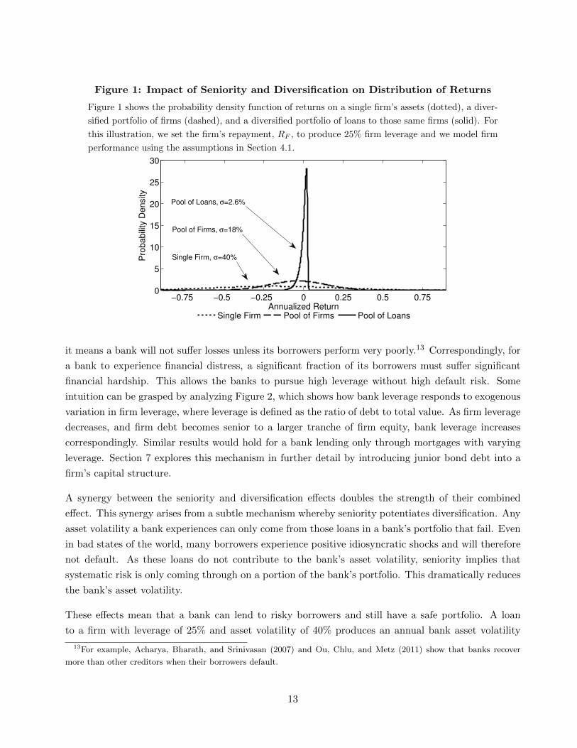
Figure 1: Impact of Seniority and Diversification on Distribution of Returns

Figure 1 shows the probability density function of returns on a single firm’s assets (dotted), a diver-

sified portfolio of firms (dashed), and a diversified portfolio of loans to those same firms (solid). For

this illustration, we set the firm’s repayment, RF , to produce 25% firm leverage and we model firm

performance using the assumptions in Section 4.1.

−0.75 −0.5 −0.25 0 0.25 0.5 0.750

5

10

15

20

25

30

Annualized Return

Pro

babili

ty D

ensity

Single Firm Pool of Firms Pool of Loans

Single Firm, σ=40%

Pool of Firms, σ=18%

Pool of Loans, σ=2.6%

it means a bank will not suffer losses unless its borrowers perform very poorly.13 Correspondingly, for

a bank to experience financial distress, a significant fraction of its borrowers must suffer significant

financial hardship. This allows the banks to pursue high leverage without high default risk. Some

intuition can be grasped by analyzing Figure 2, which shows how bank leverage responds to exogenous

variation in firm leverage, where leverage is defined as the ratio of debt to total value. As firm leverage

decreases, and firm debt becomes senior to a larger tranche of firm equity, bank leverage increases

correspondingly. Similar results would hold for a bank lending only through mortgages with varying

leverage. Section 7 explores this mechanism in further detail by introducing junior bond debt into a

firm’s capital structure.

A synergy between the seniority and diversification effects doubles the strength of their combined

effect. This synergy arises from a subtle mechanism whereby seniority potentiates diversification. Any

asset volatility a bank experiences can only come from those loans in a bank’s portfolio that fail. Even

in bad states of the world, many borrowers experience positive idiosyncratic shocks and will therefore

not default. As these loans do not contribute to the bank’s asset volatility, seniority implies that

systematic risk is only coming through on a portion of the bank’s portfolio. This dramatically reduces

the bank’s asset volatility.

These effects mean that a bank can lend to risky borrowers and still have a safe portfolio. A loan

to a firm with leverage of 25% and asset volatility of 40% produces an annual bank asset volatility

13For example, Acharya, Bharath, and Srinivasan (2007) and Ou, Chlu, and Metz (2011) show that banks recover

more than other creditors when their borrowers default.

13

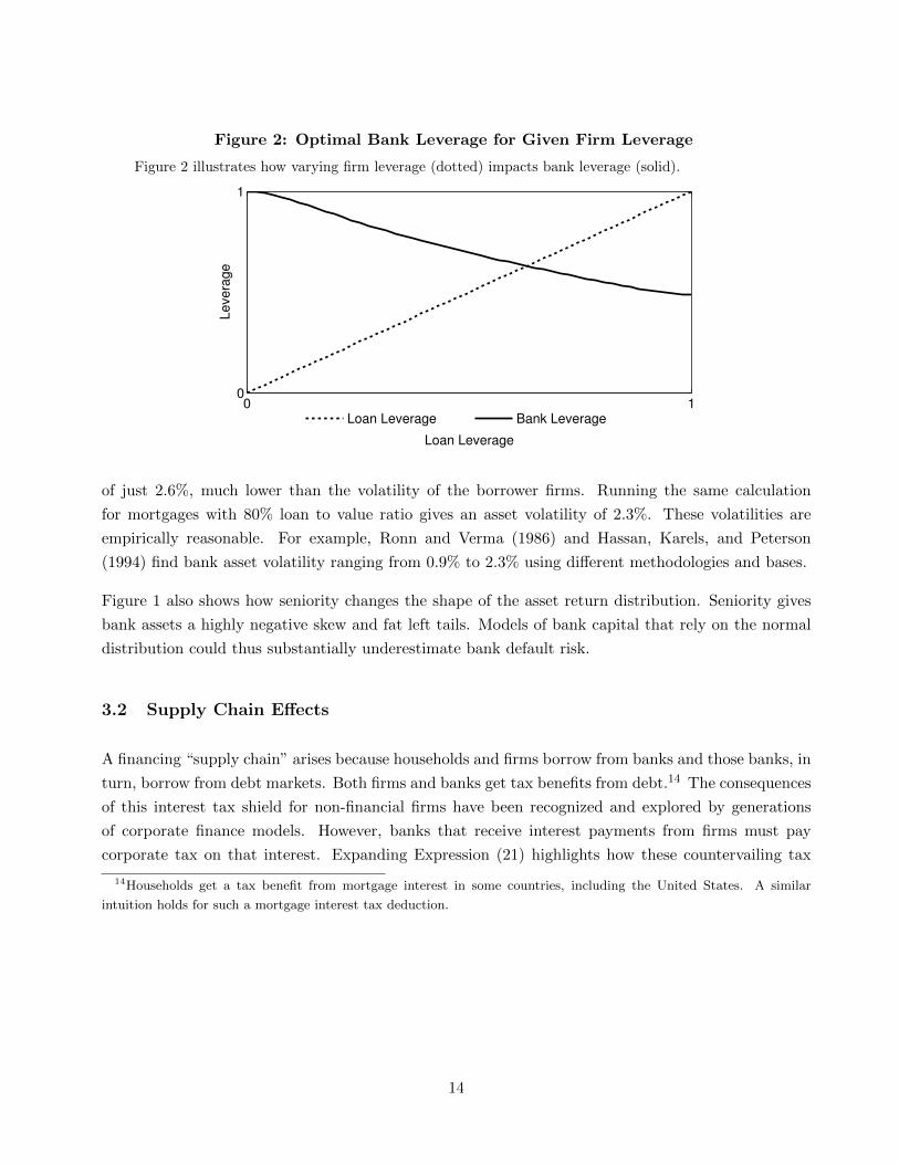
Figure 2: Optimal Bank Leverage for Given Firm Leverage

Figure 2 illustrates how varying firm leverage (dotted) impacts bank leverage (solid).

0 10

1

Loan Leverage

Levera

ge

Loan Leverage Bank Leverage

of just 2.6%, much lower than the volatility of the borrower firms. Running the same calculation

for mortgages with 80% loan to value ratio gives an asset volatility of 2.3%. These volatilities are

empirically reasonable. For example, Ronn and Verma (1986) and Hassan, Karels, and Peterson

(1994) find bank asset volatility ranging from 0.9% to 2.3% using different methodologies and bases.

Figure 1 also shows how seniority changes the shape of the asset return distribution. Seniority gives

bank assets a highly negative skew and fat left tails. Models of bank capital that rely on the normal

distribution could thus substantially underestimate bank default risk.

3.2 Supply Chain Effects

A financing “supply chain” arises because households and firms borrow from banks and those banks, in

turn, borrow from debt markets. Both firms and banks get tax benefits from debt.14 The consequences

of this interest tax shield for non-financial firms have been recognized and explored by generations

of corporate finance models. However, banks that receive interest payments from firms must pay

corporate tax on that interest. Expanding Expression (21) highlights how these countervailing tax

14Households get a tax benefit from mortgage interest in some countries, including the United States. A similar

intuition holds for such a mortgage interest tax deduction.

14

effects cause a firm’s interest tax shield to have an ambiguous effect on total tax:

VF = e−TrfE[

1− τ︸ ︷︷ ︸Unlevered value

−αF (1− τ)F iI[F i < CF

]︸ ︷︷ ︸Firm bankruptcy costs

− αBBI [B < RB]︸ ︷︷ ︸Bank bankruptcy costs

+ τ(VFD − (1− αF )(1− τ)F i)I[F i < CF

]︸ ︷︷ ︸Tax benefit of loan losses

+ τ min {RB − VBD, B − VFD}︸ ︷︷ ︸Bank interest tax shield

]. (22)

Effectively, firm interest payments constitute bank profit and thus a firm’s increased interest deduction

is a bank’s increased taxable profit. Because these effects cancel each other, the only real tax savings

come from the bank’s interest tax shield.

The observation that debt benefits originate only at the bank level is much more generic and is driven

by the fundamental asymmetry between final users of financing (“downstream” borrowers) and those

that act as intermediaries passing financing along (“upstream” borrowers). Even if the downstream

borrowers – firms – have extremely low leverage, it is still optimal for the upstream borrowers – banks

– to lever up, generate debt benefits, and pass those benefits downstream. However, if the upstream

borrowers have similarly low leverage, no benefits are generated that can be passed along and, as a

result, the downstream borrowers also do not lever up. The same logic would apply to a relationship

between a firm and its supplier that acts as a trade creditor.

This supply chain mechanism is fundamentally similar to the impact personal tax exerts on corporate

debt tax benefits. In models such as Miller (1977) or DeAngelo and Masulis (1980), firms get tax

benefits from debt but issuing debt causes a firm’s investors to pay higher personal tax. In the supply

chain model, a firm’s debt issuance increases the corporate tax of the bank holding that debt. In

both types of model, downstream borrowers cannot capture the full tax benefits of debt because of

the tax costs debt imposes on upstream debt holders. The supply chain intuition also shows that,

while traditional models of capital structure (as well as contingent-claim models of credit risk) do not

specify the identity of debt buyers, they cannot be banks or similar institutions, as these institutions

would impose their own financing frictions.

The strategic link between bank and borrower financing decisions means that these decisions can be

both strategic complements and strategic substitutes. Figure 3 highlights these interactions by showing

how firm leverage responds to exogenous variation in bank leverage.

The strategic complementarity effect arises because lower bank leverage reduces a firm’s ability to

capture the tax benefits of debt. A bank with low leverage pays substantial tax on its interest income

and must charge high interest rates to make up for that tax burden. As shown in Expression (22), a

firm’s interest payment generates a net tax benefit only to the extent that the receiver of that interest

payment can avoid paying tax on it. This supply chain effect makes bank and firm leverage strategic

complements. At the extremum, consider a firm borrowing from an all-equity bank, as shown on

15

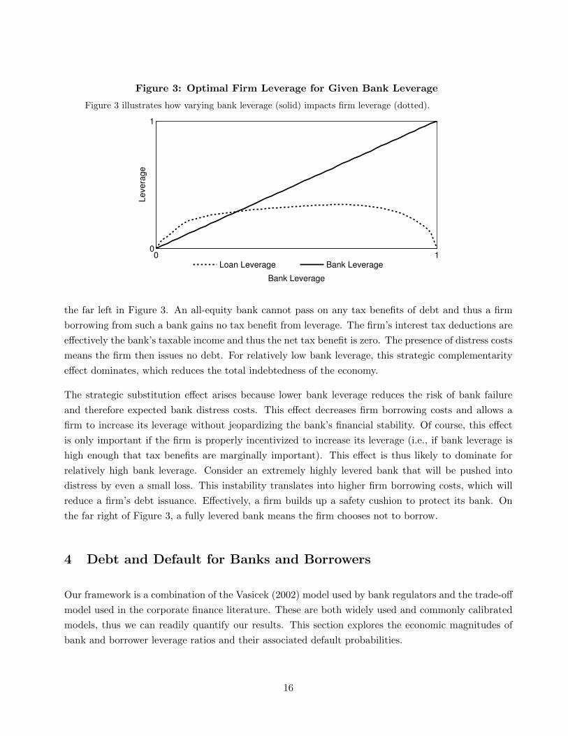
Figure 3: Optimal Firm Leverage for Given Bank Leverage

Figure 3 illustrates how varying bank leverage (solid) impacts firm leverage (dotted).

0 10

1

Bank Leverage

Levera

ge

Loan Leverage Bank Leverage

the far left in Figure 3. An all-equity bank cannot pass on any tax benefits of debt and thus a firm

borrowing from such a bank gains no tax benefit from leverage. The firm’s interest tax deductions are

effectively the bank’s taxable income and thus the net tax benefit is zero. The presence of distress costs

means the firm then issues no debt. For relatively low bank leverage, this strategic complementarity

effect dominates, which reduces the total indebtedness of the economy.

The strategic substitution effect arises because lower bank leverage reduces the risk of bank failure

and therefore expected bank distress costs. This effect decreases firm borrowing costs and allows a

firm to increase its leverage without jeopardizing the bank’s financial stability. Of course, this effect

is only important if the firm is properly incentivized to increase its leverage (i.e., if bank leverage is

high enough that tax benefits are marginally important). This effect is thus likely to dominate for

relatively high bank leverage. Consider an extremely highly levered bank that will be pushed into

distress by even a small loss. This instability translates into higher firm borrowing costs, which will

reduce a firm’s debt issuance. Effectively, a firm builds up a safety cushion to protect its bank. On

the far right of Figure 3, a fully levered bank means the firm chooses not to borrow.

4 Debt and Default for Banks and Borrowers

Our framework is a combination of the Vasicek (2002) model used by bank regulators and the trade-off

model used in the corporate finance literature. These are both widely used and commonly calibrated

models, thus we can readily quantify our results. This section explores the economic magnitudes of

bank and borrower leverage ratios and their associated default probabilities.

16

We model a bank as having three types of asset: (1) residential mortgages, (2) corporate debt, and

(3) risk-free assets such as government bonds or cash. Based on FDIC data, our benchmark case is a

bank whose assets are 60% residential mortgages, 20% corporate debt, and 20% risk-free government

securities. This simplified model excludes many bank assets such as retail exposure, commercial real

estate, and farmland loans. However, the framework can easily include any other asset class as well

as be applied to a specific bank. Our goal here is not to exactly match bank assets; rather, it is to

explore the capital structure results using a plausible bank.

4.1 Benchmark Parameter Values for Firms

Our benchmark parameter values for corporate debt are based on empirically motivated proxies.

Because many parameters of interest are challenging to estimate with good precision, we conduct

extensive comparative statics exercises.

We set the benchmark value of our firm asset correlation parameter, ρF , to 0.2.15 This is similar to

the values assumed by regulators. The Basel II (and Basel III) IRB Approach sets its loan-specific

correlation parameter, ρ, to between 0.12 and 0.24 based on the following formula:

ρ = 0.121− e−50PD

1− e−50+ 0.24

(1− 1− e−50PD

1− e−50

), (23)

where PD is the loan default probability (see paragraph 272 of BCBS (2004) for more details).16 Our

value of 0.2 is also similar to the values estimated by Lopez (2004), who uses KMV software to derive

values ranging from 0.1 to 0.3 based on firm size. However, the finance literature lacks a consensus on

the appropriate value for this parameter. For example, Dietsch and Petey (2004) find asset correlations

in the range of 0.01–0.03 for small- and medium-sized enterprises in Europe.

We set annual firm asset volatility, σF , to 0.4, a value broadly consistent with empirical estimates.

Annualizing the figures from Choi and Richardson (2008) gives volatilities in the 0.25–0.65 range,

varying with firm leverage. Schaefer and Strebulaev (2008) find asset volatility to be on the order of

0.2–0.28 for large bond issuers. While public corporate debt typically has a maturity of 7–15 years

at origination, bank debt is of shorter duration. For example, the loans studied by Roberts and Sufi

(2009) have an average time to maturity of 4 years and the BCBS (2002) prescribes a time to maturity

of 2.5 years (see paragraph 279). To be consistent with our later treatment of mortgages, we assume

a time to maturity, T , of 5 years. Time to maturity is important primarily because of its impact on

total volatility, σ√T , and so by using a longer time to maturity we are increasing the volatility of loan

collateral. This will tend to reduce both bank and firm leverage. We perform additional robustness

checks using T = 2.5. We also set the risk-free rate, rf , to 0.025.

15We use the subscripts F and A to denote parameters related to firms and residential mortgages, respectively.16The regulatory correlation is subject to a downward adjustment of up to 0.04 for loans to small firms.

17

Following estimates suggesting that the effective tax rate U.S. companies pay is less than the statutory

federal corporate tax rate of 0.35, we use a value of 0.25. For example, Graham and Tucker (2006)

show that the average S&P 500 firm paid less than 18 cents of tax per dollar of profit in each year

between 2002 and 2004 (see also Graham (1996, 2000)). We set firm and bank distress costs, αF

and αB respectively, at 0.1. For firms, this assumption is likely conservative. Some recent estimates,

such as Davydenko, Strebulaev, and Zhao (2012), find that, conditional on experiencing distress, large

firms incur sizable total distress costs of 20%–30% of asset value at the time of distress onset. In a

theoretical work, Glover (2012) suggests that distress costs can be even higher. There is little empirical

evidence on bank bankruptcy costs. James (1991) finds direct bank bankruptcy costs equal to 10% of

assets. Because distress costs are an important driver in our model, we conduct extensive robustness

tests with respect to these two parameters.

4.2 Benchmark Parameter Values for Mortgage Loans

The most popular form of mortgage loan in the U.S. is a 30-year, fixed rate mortgage with a loan

to value ratio at origination of about 80% (e.g., Bokhari, Torous, and Wheaton (2013)). This type

of mortgage features equal monthly payments and a gradually amortizing loan principal. The loan

could go into delinquency or default at any time up to its maturity or it could be refinanced at the

borrower’s choice. Default and refinancing decisions depend not only on the value of the underlying

house, but also on interest rates and the borrower’s personal situation.

These complications make modeling mortgages notoriously difficult. We therefore abstract from them

and study the “skeleton” of mortgages using the model in Section 2.1. Our goal is to provide a simple

account of how adding mortgages affects bank capital structure decisions and the consequences of those

decisions. Our model could be extended to a fuller mortgage risk model such as that of Campbell and

Cocco (2011). Below, we summarize not only our parameter assumptions but also the extent to which

these assumptions likely need to be modified in a more realistic mortgage model.

We model mortgages as 5-year term loans. Although mortgages typically have much longer maturities,

we use T = 5 because empirical evidence suggests that mortgage defaults peak in the first 5 years and

there is no refinancing risk for banks under the assumption of constant interest rates (e.g. Westerback

et al. (2011) and Figure 1.8 of International Monetary Fund (2008)). Our benchmark case uses an

80% of loan to value ratio at origination, which maps to a repayment of RA = 0.8e−Trf . Our model

assumes that the full principal is to be repaid at maturity. In practice, amortization reduces the

principal outstanding and leads to seasoned, older mortgages with lower loan to value ratios making

up a significant portion of a bank’s portfolio. Excluding the run-up to the recent financial crisis,

the average loan to value of outstanding mortgages is normally closer to 60% (e.g. p. 22 of Bullard

(2012)). The seasoning effect would make bank mortgage portfolios less risky than in our model, as

seasoned mortgages have better risk characteristics.

18

We assume that a firm defaults strategically and reneges on its debt whenever its value is below

the promised repayment. A household, on the other hand, is more likely to default as a result of

liquidity issues than for strategic reasons. Empirically, the majority of underwater homeowners do not

default, even if they are deep underwater (e.g., Figure 3 of Krainer and LeRoy (2010) or Amromin and

Paulson (2010)). At the same time, some households default even though they have positive equity in

the house. We approximate this behavior by assuming half of all the mortgages that are underwater

at maturity default and other mortgages do not. The cost of foreclosure, αA, is assumed to be 0.25.

This matches empirical studies such as the one by Qi and Yang (2009) who find an average loss of

25% for defaulting mortgages, where the house value is equal to the mortgage debt.

We use σA = 0.25 for house price volatility. This is roughly in line with the levels suggested by

Zhou and Haurin (2010), who find volatility ranging from 13-25%. The Basel regulation contains no

guidance on house price volatility. We assume that the correlation between the price movements of

different houses in a bank’s mortgage portfolio is ρA = 0.2.17 The Basel regulation assigns a lower

value of 0.15. We use a higher value of 0.2 in order to match the recent U.S. experience of higher

correlation (e.g., Cotter, Gabriel, and Roll (2011)). To see how these assumptions perform over the

long run, it is useful to conduct a long-term volatility exercise. Our values of σA = 0.25 and ρA = 0.2

produce a 5-year index volatility of 25% which is close to the 21% 5-year volatility of Case-Shiller

index. A 2008-style housing crisis with a 40% 5-year house price decline occurs approximately once

per century under our model which again matches the Case-Shiller index.

Beyond the characteristics of mortgage loans, it is important to comment on how banks hold mortgages.

Guarantees and securitization are defining features of the U.S. mortgage market. More than half of

U.S. mortgages are guaranteed by government-sponsored enterprises, such as Fannie Mae or Freddie

Mac, or by government agencies, such as the Federal Housing Administration or the Department

of Veteran’s Affairs (e.g., Congressional Budget Office (2010)). The majority of these guaranteed

mortgages, along with many mortgages that lack such guarantees, are then packaged into mortgage-

backed securities and sold. If the bank takes the securitized or guaranteed mortgages off its balance

sheet, the model needs no adjustment. If these structures remain on a bank’s balance sheet, they can

alter that bank’s risk. Guarantees can dramatically reduce bank risk as the credit risk is borne by the

guarantor. Securitizations can reduce or concentrate risk, depending on their structure and the risk

the bank chooses to retain. Our model assumes that the bank retains no interest in any securitizations

and no guaranteed assets; however, the model could be extended to cover a richer case.

17Like the Basel IRB Framework, our analysis implicitly uses a single factor model. This means that house prices

co-move with firm asset values as both are exposed to the bank risk factor. Our framework can be easily extended to

include multiple factors.

19

4.3 Benchmark Estimates

Highly levered banks arise from our base case parameter assumptions, as well as plausible parameter

variations. Table 2 shows the capital structure and default risk implications of our model for a variety

of parameter values. The first two columns consider a firm borrowing from a bank and show the firm

market leverage ratio, VFD/(VFE + VFD), and the associated annual firm default probability. The

next two columns show the capital structure and default rate of the bank, where the bank’s market

leverage ratio is given by VBD/(VBE+VBD).18 For comparison, the final two columns show the capital

structure and default probability of a firm that issues bonds in the public market and does not borrow

from the bank. Three results immediately stand out.

First, bank leverage is indeed very high. Our benchmark case yields banks with 86% leverage, a value

that would be extremely high for a non-financial firm (indeed, a non-financial firm with such leverage

would almost automatically be regarded as in distress) but in line with the empirical evidence on the

capital structure of financial firms. For example, Federal Deposit Insurance Corporation (FDIC) data

shows that aggregate bank book leverage has been 87%–95% for the past 80 years.19 Furthermore,

all of the parameter variations in Table 2 produce high bank leverage. As discussed in Section 3, this

result is driven by the confluence of seniority and diversification effects which dramatically reduces

bank risk and allows banks to afford high leverage. A good illustration of the relative safety of banks is

that in our base case, banks have an annual default rate of only 0.18%, which is close to the historical

U.S. bank failure rate of 0.42%.20

Second, firm leverage is substantially lower than bank leverage, as has been widely empirically doc-

umented. The quasi-market leverage ratio for U.S. public firms between 1962 and 2009 averaged

25%–30%, with more than 20% of firms having less than 5% leverage (e.g., Strebulaev and Yang

(2013)). A tendency of non-financial firms to exhibit low leverage and the failure of many standard

models to explain such low leverage is known as the low-leverage puzzle and has sprung its own stream

of research (e.g., Leland (1994, 1998); Goldstein, Ju, and Leland (2001); Morellec (2004); Ju, Parrino,

Poteshman, and Weisbach (2005); Strebulaev (2007)). For the benchmark parameter estimates, our

model produces firm leverage of 30%, in line with empirical evidence but substantially smaller than in

most trade-off models. What can explain an almost 60% difference between bank and firm leverage?

Obviously, firms do not enjoy the same diversification and seniority protection that banks do. The

low leverage of firms arises from two further reasons. First, a firm borrowing through a bank bears

18A zero profit bank has equal book and market values for both bank equity and bank assets. Section 7 explores

profitable banks and shows similar results.19Authors’ estimates based on historical FDIC data, which are publicly available from http://www2.fdic.gov/hsob/

HSOBRpt.asp.20Authors estimates based on FDIC data, which are publicly available from http://www2.fdic.gov/hsob/. From 1934

to 2012, the FDIC reports 4033 bank failures out of 963,939 bank-year observations. Note that adding deposit insurance

or bailouts to our model brings the bank default rate up to that level. Refer to Section 5 for more details.

20

that bank’s default costs, and so borrows less to protect the bank (the strategic substitution effect).

Second, the borrowing firm captures only some of the tax benefits of debt as the rest are lost through

the bank’s tax costs – the financing supply chain is not completely frictionless.

The third result is that firms that borrow through banks have lower leverage (30%) than firms with

direct access to the capital markets (51%).21 This is again in line with empirical evidence, such as

Faulkender and Wang (2006) who show that among firms with positive debt, those with bond market

access have higher leverage (28.5%) than those without (20.5%). A firm borrowing through a bank

bears some of that bank’s capital structure costs and so borrows less. Beyond our model, this effect

could also hold for mortgages. Mortgages that are securitized or guaranteed can offset the credit risk

they impose on the bank, which would result in higher mortgage debt and lower mortgage interest

rates.

Beyond our base case bank, bank leverage is high for a variety of borrowers and types of loans, as

illustrated by Table 3. Higher borrower leverage results in lower bank leverage, but the bank still

pursues high leverage for variety of portfolio compositions.

If bank leverage cannot adjust in response to borrower leverage, bank defaults become more common.

Figure 4 holds bank leverage fixed and looks at how borrower leverage impacts bank default proba-

bilities. Holding bank leverage fixed at 85% and increasing firm leverage from 30% to 60% causes the

1-year default probability of a bank that lends to firms to increase sevenfold, from 0.89% to 6.24%.

Holding bank leverage at 90% and increasing mortgage loan to value ratios from 80% to 100% similarly

causes the default probability of an all-mortgage bank to increase to from 0.11% to 1.20%. Both high

firm leverage and high bank leverage are associated with more frequent bank defaults. As a potential

illustration, the run-up to the recent financial crisis was associated with a dramatic increase in the

leverage of households. Banks that failed to model such an increase in leverage would have been

extremely vulnerable to systemic shocks due to their unexpectedly inadequate seniority.

4.4 Impact of Systematic Risk

Varying the extent to which risk is systematic has a nonmonotonic effect on bank and firm leverage, as

illustrated by Figure 5a. Low systematic risk leads to highly levered banks and firms because better

diversified exposures reduce systemic risk costs. In the extreme example of ρ = 0, the Diamond (1984)

case, banks are optimally fully levered as their risk is completely diversified. Adding systematic risk

causes a gradual decrease in both firm and bank leverage. There are two related effects. First, banks

reduce their leverage to protect against default as increasing correlation raises their portfolio volatility.

21Static trade-off models of capital structure typically result in much higher leverage. In these models, debt is issued as

a perpetuity, while in our case the tax benefits effectively accumulate over a relatively short period. Thus, our modeling

of debt maturity is closer to dynamic capital structure models that produce much lower leverage.

21

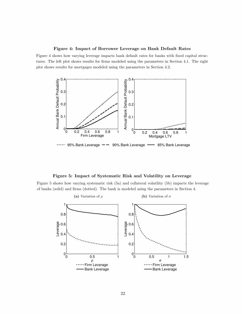
Figure 4: Impact of Borrower Leverage on Bank Default Rates

Figure 4 shows how varying leverage impacts bank default rates for banks with fixed capital struc-

tures. The left plot shows results for firms modeled using the parameters in Section 4.1. The right

plot shows results for mortgages modeled using the parameters in Section 4.2.

0 0.2 0.4 0.6 0.8 10

0.1

0.2

0.3

0.4

Firm Leverage

Annual B

ank D

efa

ult P

robabili

ty

0 0.2 0.4 0.6 0.8 10

0.1

0.2

0.3

0.4

Mortgage LTV

Annual B

ank D

efa

ult P

robabili

ty

95% Bank Leverage 90% Bank Leverage 85% Bank Leverage

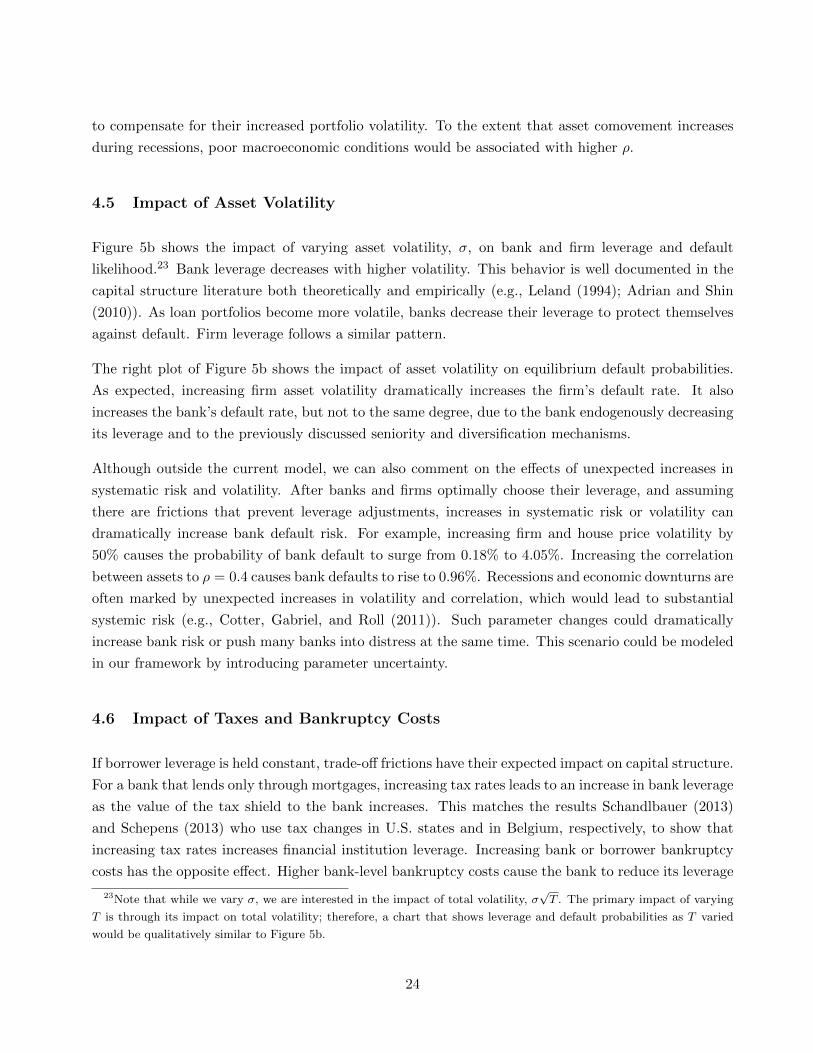
Figure 5: Impact of Systematic Risk and Volatility on Leverage

Figure 5 shows how varying systematic risk (5a) and collateral volatility (5b) impacts the leverage

of banks (solid) and firms (dotted). The bank is modeled using the parameters in Section 4.

(a) Variation of ρ

0 0.5 10

0.2

0.4

0.6

0.8

1

ρ

Levera

ge

Firm Leverage

Bank Leverage

0 0.5 1 1.50

0.2

0.4

0.6

0.8

1

σ

Levera

ge

Firm Leverage

Bank Leverage

(b) Variation of σ

0 0.5 10

0.2

0.4

0.6

0.8

1

ρ

Levera

ge

Firm Leverage

Bank Leverage

0 0.5 1 1.50

0.2

0.4

0.6

0.8

1

σ

Levera

ge

Firm Leverage

Bank Leverage

22

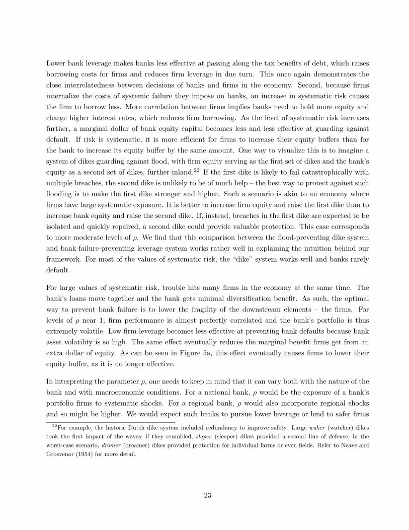
Lower bank leverage makes banks less effective at passing along the tax benefits of debt, which raises

borrowing costs for firms and reduces firm leverage in due turn. This once again demonstrates the

close interrelatedness between decisions of banks and firms in the economy. Second, because firms

internalize the costs of systemic failure they impose on banks, an increase in systematic risk causes

the firm to borrow less. More correlation between firms implies banks need to hold more equity and

charge higher interest rates, which reduces firm borrowing. As the level of systematic risk increases

further, a marginal dollar of bank equity capital becomes less and less effective at guarding against

default. If risk is systematic, it is more efficient for firms to increase their equity buffers than for

the bank to increase its equity buffer by the same amount. One way to visualize this is to imagine a

system of dikes guarding against flood, with firm equity serving as the first set of dikes and the bank’s

equity as a second set of dikes, further inland.22 If the first dike is likely to fail catastrophically with

multiple breaches, the second dike is unlikely to be of much help – the best way to protect against such

flooding is to make the first dike stronger and higher. Such a scenario is akin to an economy where

firms have large systematic exposure. It is better to increase firm equity and raise the first dike than to

increase bank equity and raise the second dike. If, instead, breaches in the first dike are expected to be

isolated and quickly repaired, a second dike could provide valuable protection. This case corresponds

to more moderate levels of ρ. We find that this comparison between the flood-preventing dike system

and bank-failure-preventing leverage system works rather well in explaining the intuition behind our

framework. For most of the values of systematic risk, the “dike” system works well and banks rarely

default.

For large values of systematic risk, trouble hits many firms in the economy at the same time. The

bank’s loans move together and the bank gets minimal diversification benefit. As such, the optimal

way to prevent bank failure is to lower the fragility of the downstream elements – the firms. For

levels of ρ near 1, firm performance is almost perfectly correlated and the bank’s portfolio is thus

extremely volatile. Low firm leverage becomes less effective at preventing bank defaults because bank

asset volatility is so high. The same effect eventually reduces the marginal benefit firms get from an

extra dollar of equity. As can be seen in Figure 5a, this effect eventually causes firms to lower their

equity buffer, as it is no longer effective.

In interpreting the parameter ρ, one needs to keep in mind that it can vary both with the nature of the

bank and with macroeconomic conditions. For a national bank, ρ would be the exposure of a bank’s

portfolio firms to systematic shocks. For a regional bank, ρ would also incorporate regional shocks

and so might be higher. We would expect such banks to pursue lower leverage or lend to safer firms

22For example, the historic Dutch dike system included redundancy to improve safety. Large waker (watcher) dikes

took the first impact of the waves; if they crumbled, slaper (sleeper) dikes provided a second line of defense; in the

worst-case scenario, dromer (dreamer) dikes provided protection for individual farms or even fields. Refer to Neave and

Grosvenor (1954) for more detail.

23

to compensate for their increased portfolio volatility. To the extent that asset comovement increases

during recessions, poor macroeconomic conditions would be associated with higher ρ.

4.5 Impact of Asset Volatility

Figure 5b shows the impact of varying asset volatility, σ, on bank and firm leverage and default

likelihood.23 Bank leverage decreases with higher volatility. This behavior is well documented in the

capital structure literature both theoretically and empirically (e.g., Leland (1994); Adrian and Shin

(2010)). As loan portfolios become more volatile, banks decrease their leverage to protect themselves

against default. Firm leverage follows a similar pattern.

The right plot of Figure 5b shows the impact of asset volatility on equilibrium default probabilities.

As expected, increasing firm asset volatility dramatically increases the firm’s default rate. It also

increases the bank’s default rate, but not to the same degree, due to the bank endogenously decreasing

its leverage and to the previously discussed seniority and diversification mechanisms.

Although outside the current model, we can also comment on the effects of unexpected increases in

systematic risk and volatility. After banks and firms optimally choose their leverage, and assuming

there are frictions that prevent leverage adjustments, increases in systematic risk or volatility can

dramatically increase bank default risk. For example, increasing firm and house price volatility by

50% causes the probability of bank default to surge from 0.18% to 4.05%. Increasing the correlation

between assets to ρ = 0.4 causes bank defaults to rise to 0.96%. Recessions and economic downturns are

often marked by unexpected increases in volatility and correlation, which would lead to substantial

systemic risk (e.g., Cotter, Gabriel, and Roll (2011)). Such parameter changes could dramatically

increase bank risk or push many banks into distress at the same time. This scenario could be modeled

in our framework by introducing parameter uncertainty.

4.6 Impact of Taxes and Bankruptcy Costs

If borrower leverage is held constant, trade-off frictions have their expected impact on capital structure.

For a bank that lends only through mortgages, increasing tax rates leads to an increase in bank leverage

as the value of the tax shield to the bank increases. This matches the results Schandlbauer (2013)

and Schepens (2013) who use tax changes in U.S. states and in Belgium, respectively, to show that

increasing tax rates increases financial institution leverage. Increasing bank or borrower bankruptcy

costs has the opposite effect. Higher bank-level bankruptcy costs cause the bank to reduce its leverage

23Note that while we vary σ, we are interested in the impact of total volatility, σ√T . The primary impact of varying

T is through its impact on total volatility; therefore, a chart that shows leverage and default probabilities as T varied

would be qualitatively similar to Figure 5b.

24

to avoid those. Higher borrower-level bankruptcy costs also reduce bank leverage, as higher bankruptcy

costs incre ase bank bankruptcy risk.

If borrower leverage is endogenous, these effect can vary. Higher tax rates cause firms to take on higher

leverage. That increases the amount of risk the bank has in its portfolio. Thus, increasing tax rates

have an indeterminate effect on bank leverage. Bank-level bankruptcy costs decrease both bank and

firm leverage. Borrower-level bankruptcy costs decrease borrower level. Bank leverage decreases for

most parameter values; however, very high borrower-level bankruptcy costs can dramatically decrease

borrower leverage which causes a corresponding increase in bank leverage. Note that even for very

high bank bankruptcy costs, the bank still opts for relatively high debt levels due to the supply chain

mechanism and seniority and diversification effects.

5 Moral Hazard and Leverage

Government interventions such as bailouts and deposit insurance subsidize banks in financial distress.

We find that such interventions can have a substantial impact, not only on a bank’s behavior but also

on the debt decisions of its borrowers. Expectations of government support provide banks with bad

incentives, as well as changing the way banks price risk in a way that pushes borrowers toward higher

leverage. In Section 6, we extend this analysis to incorporate bank capital regulation.

5.1 Deposit Insurance

Government-backed deposit insurance protects bank depositors from the costs of bank failure. Most

developed countries have schemes of this sort to help prevent bank failures. In the U.S., the FDIC

is a deposit insurance program guaranteed by the federal government in which all deposit-taking

institutions participate. We set out a simplified model of deposit insurance based on the U.S. system.

Let D be the amount of insured depositors a bank has at date 0. Because insured depositors are

guaranteed to receive their investment back, their debt is risk-free and at time T they are owed DeTrf

by the bank. We assume that payments to insured depositors make up a constant portion of the

bank’s repayment, DeTrf = γVBD.24

The class of insured depositors can be thought of as a separate class of debt. The payout to the

residual debt holders (uninsured depositors and other creditors) is RB − DeTrf if the bank survives

24Additionally, we limit the bank’s promised repayment to be equal to the value of its loans if those loans were held

by a tax-free investor. Similar results arise if we assume D is proportional to the bank’s assets or liabilities or impose

other reasonable limits on D.

25

and max{

0, (1− αB)B −DeTrf}

if the bank defaults.25 The value of the residual debt holders’ claim

at date 0 is

(1− γ)VBD = e−Trf (RB −DeTrf )P [B ≥ RB]

+ e−TrfE[max

{0,((1− αB)B −DeTrf

)}I [B < RB]

]. (24)

Adding this to the value of insured deposits, the total value of the bank’s debt is

VBD = e−TrfRBP [B ≥ RB] + e−TrfE [(1− αB)I [B < RB]]︸ ︷︷ ︸Debt value without deposit insurance

+ e−TrfE[max

{0, DeTrf − (1− αB)B

}]︸ ︷︷ ︸Value of deposit insurance

. (25)

Figure 6 shows the impact of varying the amount of insured deposits on the leverage and default

likelihood of banks and firms. Two results can be gleaned from the figure. First, moderate levels of

insured deposits cause only slight changes in capital structure. Deposit insurance is essentially a deep

out of the money put option on the bank’s value. Bank asset volatility is low, which means losses

large enough to trigger deposit insurance are unlikely and this put option has little value. As with the

deductibles seen in personal insurance markets, forcing the claimant (the bank) to pay the first dollar

of losses (using equity and uninsured debt) dramatically reduces moral hazard.

Second, high levels of insured deposits cause the bank to pursue high-risk strategies by leveraging

to the hilt and gambling on excessively risky loans. Our benchmark bank switches to a risk-seeking

strategy that exploits the government guarantee when insured deposits make up more than 92% of its

liabilities. Empirical evidence supports the idea that some banks pursue a risky strategy while others

pursue safer strategies. Lambert, Noth, and Schuwer (2012) find that while a plausibly exogenous

increase in loan risk causes well-capitalized banks to increase their capital buffers and shift into less

risky loans, poorly capitalized banks are less likely to follow this path. Increasing borrower asset

volatility or the correlation between borrowers makes banks more willing to gamble. For example,

increasing σ and ρ by 50% decreases the critical level of deposit insurance to 84%.

According to FDIC data for 2013:Q1, the median bank in the U.S. has insured deposits equal to 79%

of liabilities, with a 75th percentile bank having insured deposits equal to 85% of liabilities.26 Our

model suggests that this level of insured deposits is unlikely to generate substantial moral hazard for

a representative bank. However, 7% of banks have insured deposits that make up in excess of 95% of

25In the U.S., uninsured deposits are paid out pari passu with insured deposits, with insured depositors then made

whole by the FDIC. This means that uninsured deposits increase the value of deposit insurance to failing banks. We

ignore this effect and assume that insured deposits are paid before uninsured deposits.26Authors’ estimates based on bank level FDIC data, which are publicly available from http://www2.fdic.gov/idasp/

warp download all.asp.

26

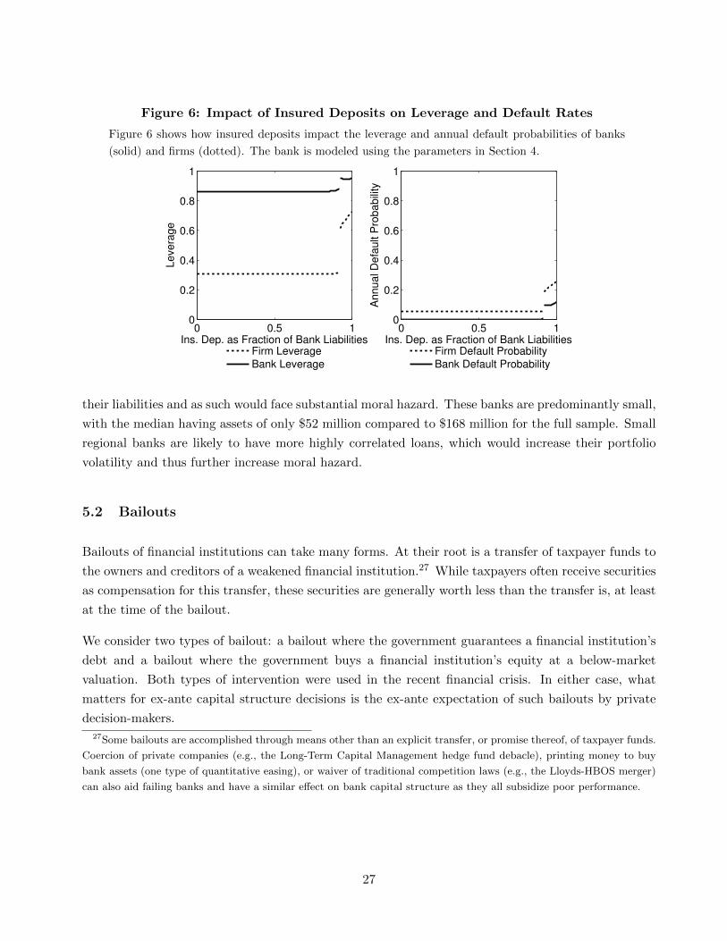
Figure 6: Impact of Insured Deposits on Leverage and Default Rates

Figure 6 shows how insured deposits impact the leverage and annual default probabilities of banks

(solid) and firms (dotted). The bank is modeled using the parameters in Section 4.

0 0.5 10

0.2

0.4

0.6

0.8

1

Ins. Dep. as Fraction of Bank Liabilities

Levera

ge

Firm Leverage

Bank Leverage

0 0.5 10

0.2

0.4

0.6

0.8

1

Ins. Dep. as Fraction of Bank Liabilities

Annual D

efa

ult P

robabili

ty

Firm Default Probability

Bank Default Probability

their liabilities and as such would face substantial moral hazard. These banks are predominantly small,

with the median having assets of only $52 million compared to $168 million for the full sample. Small

regional banks are likely to have more highly correlated loans, which would increase their portfolio

volatility and thus further increase moral hazard.

5.2 Bailouts

Bailouts of financial institutions can take many forms. At their root is a transfer of taxpayer funds to

the owners and creditors of a weakened financial institution.27 While taxpayers often receive securities

as compensation for this transfer, these securities are generally worth less than the transfer is, at least

at the time of the bailout.

We consider two types of bailout: a bailout where the government guarantees a financial institution’s

debt and a bailout where the government buys a financial institution’s equity at a below-market

valuation. Both types of intervention were used in the recent financial crisis. In either case, what

matters for ex-ante capital structure decisions is the ex-ante expectation of such bailouts by private

decision-makers.

27Some bailouts are accomplished through means other than an explicit transfer, or promise thereof, of taxpayer funds.

Coercion of private companies (e.g., the Long-Term Capital Management hedge fund debacle), printing money to buy

bank assets (one type of quantitative easing), or waiver of traditional competition laws (e.g., the Lloyds-HBOS merger)

can also aid failing banks and have a similar effect on bank capital structure as they all subsidize poor performance.

27

5.2.1 Debt Guarantees

Market participants may expect that the government will step in and pay the debts of a distressed

bank. This response may be contingent upon macroeconomic, macrofinancial, and political concerns.

Further, what matters is not the government’s present choice of action but the government’s expected

action in the future when the bank is near default. Abstracting beyond those considerations, sup-

pose that the market’s expectation is that with some probability, θ, the government will step in and

guarantee a failing bank’s debt; otherwise that bank will be allowed to fail.

If the government intervenes, the government takes over the failing bank and pays the bank’s creditors

their promised repayment, RB. The expectation of this type of bailout increases the bank’s date-0

debt value:

VBD = e−TrfRBP [B ≥ RB] + e−TrfE[θVBDe

Trf + (1− θ)(1− τ)(1− αB)BI [B < RB]]. (26)

Expectations of such a debt guarantee create moral hazard for the bank at the time of a capital

structure decision because the bank is subsidized in the states of the world where it defaults. This

gives the bank an incentive to issue more debt in order to take advantage of that potential subsidy.

Figure 7 illustrates how bank leverage increases as bailouts become more likely. If bailouts are seen as

very likely (above about a 52% probability for our benchmark set of parameters), the bank experiences

extreme moral hazard. At this point, as the gains from taxpayer-subsidized gambling overwhelm the

gains from legitimate lending, the bank chooses to pursue extremely high leverage and lend to very

risky firms. Bank default risk quadruples if the probability of a bailout is 50%. If the probability rises

to 75%, the likelihood of bank default increases by a factor of 50 and the bank shifts to a risk-seeking

strategy with very frequent defaults.

5.2.2 Equity Injections

Alternatively, market participants may expect a bailout in the form of the purchase of a bank’s equity

at an above-market price. Regulators frequently employed this form of bailout during the recent

financial crisis. For example, a number of U.S. financial institutions, such as Citigroup and Bank of

America, participated in the Troubled Asset Relief Program, in which the U.S. government purchased

common and preferred equity from distressed institutions. The Royal Bank of Scotland received

massive injections of equity in dire circumstances and is still majority owned, at the time of writing,

by the U.K. government.

We model this form of bailout as follows. Assume that if a bank’s portfolio value is so low that it would

otherwise default, the government purchases a fraction of the bank’s equity at an above-market price.

This equity injection occurs only if the bank will become solvent after receiving the cash. Suppose

28

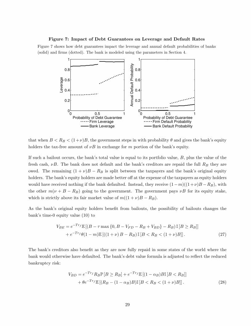
Figure 7: Impact of Debt Guarantees on Leverage and Default Rates

Figure 7 shows how debt guarantees impact the leverage and annual default probabilities of banks

(solid) and firms (dotted). The bank is modeled using the parameters in Section 4.

0 0.5 10

0.2

0.4

0.6

0.8

1

Probability of Debt Guarantee

Levera

ge

Firm Leverage

Bank Leverage

0 0.5 10

0.2

0.4

0.6

0.8

1

Probability of Debt Guarantee

Annual D

efa

ult P

robabili

ty

Firm Default Probability

Bank Default Probability

that when B < RB < (1+ν)B, the government steps in with probability θ and gives the bank’s equity

holders the tax-free amount of νB in exchange for m portion of the bank’s equity.

If such a bailout occurs, the bank’s total value is equal to its portfolio value, B, plus the value of the

fresh cash, νB. The bank does not default and the bank’s creditors are repaid the full RB they are

owed. The remaining (1 + ν)B − RB is split between the taxpayers and the bank’s original equity

holders. The bank’s equity holders are made better off at the expense of the taxpayers as equity holders

would have received nothing if the bank defaulted. Instead, they receive (1−m)((1 +ν)B−RB), with

the other m(ν + B − RB) going to the government. The government pays νB for its equity stake,

which is strictly above its fair market value of m((1 + ν)B −RB).

As the bank’s original equity holders benefit from bailouts, the possibility of bailouts changes the

bank’s time-0 equity value (10) to

VBE = e−TrfE [(B − τ max {0, B − VFD −RB + VBD} −RB) I [B ≥ RB]]

+ e−Trf θ(1−m)E [((1 + ν)B −RB) I [B < RB < (1 + ν)B]] . (27)

The bank’s creditors also benefit as they are now fully repaid in some states of the world where the

bank would otherwise have defaulted. The bank’s debt value formula is adjusted to reflect the reduced

bankruptcy risk:

VBD = e−TrfRBP [B ≥ RB] + e−TrfE [(1− αB)BI [B < RB]]

+ θe−TrfE [(RB − (1− αB)B)I [B < RB < (1 + ν)B]] . (28)

29

Figure 8: Impact of Equity Injections on Leverage and Default Rates

Figure 8 shows how the size of a potential equity injection, ν, impacts the leverage and annual

default probabilities of banks (solid) and firms (dotted). The bank is modeled using the parameters

in Sections 4 and 5.2.2.

0 0.05 0.10

0.2

0.4

0.6

0.8

1

Equity Injection Size

Levera

ge

Firm Leverage

Bank Leverage

0 0.05 0.10

0.2

0.4

0.6

0.8

1

Equity Injection Size

Annual D

efa

ult P

robabili

ty

Firm Default Probability

Bank Default Probability

This form of bailout also creates moral hazard. Figure 8 illustrate the leverage in the economy as

the size of the equity injection varies from 0 to 0.1. For this illustration, we hold the probability of a

bailout, θ, and the equity stake taken by the government, m, fixed at 0.5. As the size of the potential

equity injection increases, the bank increases its own leverage from 86% to 92%. Equity injections

subsidize risk taking and failure, and so banks take more risk. For any given leverage level, increasing

the size or frequency of equity injections reduces the bank’s default likelihood, as the bank is more

likely to get an equity injection that allows it to repay that debt. However, the possibility of bailouts

causes the bank to take so much additional risk that the bank’s default likelihood actually increases,

despite the bailout saving the bank from failure in some states of the world. Changing the other

bailout parameters has a similar effect to changing the size of the bailout: Increasing the probability

of a bailout or decreasing the equity stake taken by the government both increase bank leverage.

Both the bailouts we have considered generate moral hazard for financial institutions. Small interven-

tions have only a very small effect on risk taking, but sufficiently high bailout expectations cause the

bank to pursue destructive risk-seeking strategies. Government interventions may be optimal ex-post

to avoid the social costs of bank bankruptcy; however, at least without capital regulation, the ex-ante

expectation of bailouts leads to higher bank leverage and so interventions end up increasing the rate

of bank failure.

30

6 Capital Regulation

Capital regulation that restricts bank financing is a key weapon regulators use to combat bank risk

taking. Preventing a bank from issuing excessive debt reduces its incentive to risk-shift and insulates

its creditors and depositors from loss. Capital regulation policies, as well as their cost and impact,

have been at the center of recent debates by both practitioners and academics. We find that while

capital regulation reduces bank leverage, it can increase borrower leverage by changing the way banks

price risk and thus lead to more borrower defaults.

While capital regulation takes many forms, the international standards laid out in Basel II and those

proposed in Basel III form widely accepted benchmarks. Basel II, and now Basel III, lays out dif-

ferent capital regulation guidelines for banks of different sizes. The capital requirements for smaller

and less sophisticated banks are set using the Standardized Approach, which uses simple risk weights

for different types of assets. Larger banks are subject to the IRB Approach, where a bank’s equity

requirements are calculated using outputs from that bank’s own models.28 In the following sections,

we apply these two regulatory approaches to our model and examine how effectively these regulations

combat the incentive problems introduced by bailouts and deposit insurance. These regulatory struc-

tures are complicated and thus we focus on equity standards and use simplified models; however, our

results are very general.

6.1 Basel Capital Regulation: Standardized Approach

Under the Standardized Approach of Basel II and III, banks need to hold equity capital equal to a

constant fraction of their risk-weighted assets. We model this type of regulation by assuming a bank

must have equity capital, VBE , in excess of h portion of its risk-weighted assets, so that

VBE ≥ VB × w × h, (29)

where VB is the bank’s asset value, w is the bank’s risk weight, and h is the capital requirement.

The BCBS (2013) sets out a so-called Standardized Approach that assigns a bank a risk weight based

on the assets in its portfolio. For example, residential mortgages are placed into buckets based on loan

to value ratio and loan properties and given risk weights of 35–200% and corporate debt is given a

risk weight varying from 20–150% depending on rating.29 The total risk weight of the bank’s assets

28The U.S. implementation of Basel III requires that the largest banks use the IRB Approach in addition to the Stan-

dardized Approach. See the report by the Office of the Comptroller (2013) for more details on the U.S. implementation

of Basel III.29Note that capital regulation is usually written in terms of the book value of assets and the book value of equity.

Under our model, the time-0 book values and market values are equal for both equity and assets as the bank is zero

profit.

31

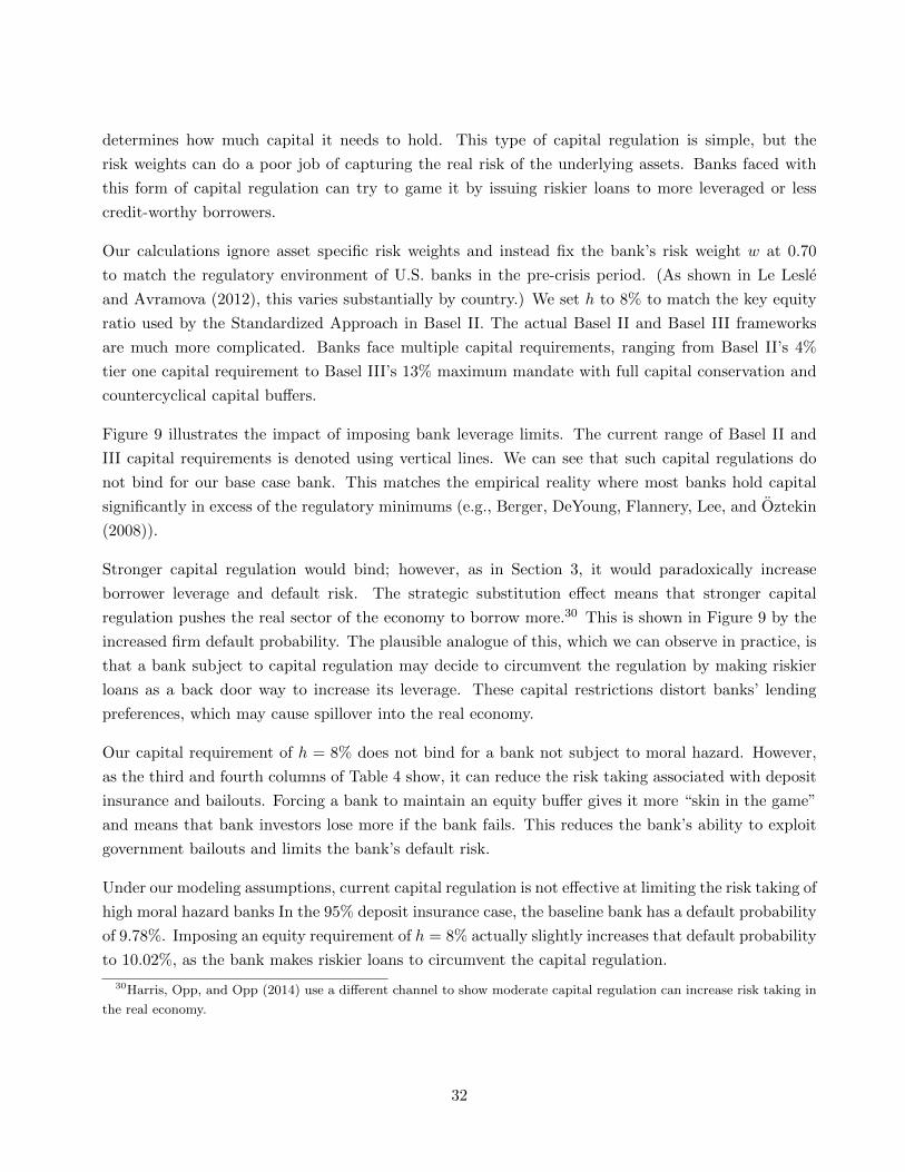
determines how much capital it needs to hold. This type of capital regulation is simple, but the

risk weights can do a poor job of capturing the real risk of the underlying assets. Banks faced with

this form of capital regulation can try to game it by issuing riskier loans to more leveraged or less

credit-worthy borrowers.

Our calculations ignore asset specific risk weights and instead fix the bank’s risk weight w at 0.70

to match the regulatory environment of U.S. banks in the pre-crisis period. (As shown in Le Lesle

and Avramova (2012), this varies substantially by country.) We set h to 8% to match the key equity

ratio used by the Standardized Approach in Basel II. The actual Basel II and Basel III frameworks

are much more complicated. Banks face multiple capital requirements, ranging from Basel II’s 4%

tier one capital requirement to Basel III’s 13% maximum mandate with full capital conservation and

countercyclical capital buffers.

Figure 9 illustrates the impact of imposing bank leverage limits. The current range of Basel II and

III capital requirements is denoted using vertical lines. We can see that such capital regulations do

not bind for our base case bank. This matches the empirical reality where most banks hold capital

significantly in excess of the regulatory minimums (e.g., Berger, DeYoung, Flannery, Lee, and Oztekin

(2008)).

Stronger capital regulation would bind; however, as in Section 3, it would paradoxically increase

borrower leverage and default risk. The strategic substitution effect means that stronger capital

regulation pushes the real sector of the economy to borrow more.30 This is shown in Figure 9 by the

increased firm default probability. The plausible analogue of this, which we can observe in practice, is

that a bank subject to capital regulation may decide to circumvent the regulation by making riskier

loans as a back door way to increase its leverage. These capital restrictions distort banks’ lending

preferences, which may cause spillover into the real economy.

Our capital requirement of h = 8% does not bind for a bank not subject to moral hazard. However,

as the third and fourth columns of Table 4 show, it can reduce the risk taking associated with deposit

insurance and bailouts. Forcing a bank to maintain an equity buffer gives it more “skin in the game”

and means that bank investors lose more if the bank fails. This reduces the bank’s ability to exploit

government bailouts and limits the bank’s default risk.

Under our modeling assumptions, current capital regulation is not effective at limiting the risk taking of

high moral hazard banks In the 95% deposit insurance case, the baseline bank has a default probability

of 9.78%. Imposing an equity requirement of h = 8% actually slightly increases that default probability

to 10.02%, as the bank makes riskier loans to circumvent the capital regulation.

30Harris, Opp, and Opp (2014) use a different channel to show moderate capital regulation can increase risk taking in

the real economy.

32

Figure 9: Impact of Bank Leverage Limits on Leverage and Default Rates

Figure 9 shows how capital regulation that mandates an equity capital to asset ratio above h impacts

the leverage and annual default probabilities of banks (solid) and firms (dotted). The parameter

values are rf = 0.05, σ = 0.4, ρ = 0.2, τ = 0.25, αF = αB = 0.1, T = 2.5. The vertical lines denote

bounds on the current Basel capital requirements which range from h = 4% to h = 13%. The bank

is modeled using the parameters in Section 4.

0 4 8 13 20 30 40 500

0.2

0.4

0.6

0.8

1

Equity Requirement h (%)

Levera

ge

Firm Leverage

Bank Leverage

0 8 25 500

0.2

0.4

0.6

0.8

1

Equity Requirement h (%)A

nnual D

efa

ult P

robabili

ty

Firm Default Probability

Bank Default Probability

6.2 Basel Capital Regulation: Internal Ratings-Based Approach

Simple leverage limits may push banks toward risky lending. One countermeasure is to risk-weight

assets. Basel II and III include this type of capital regulation as an option for banks. The risk-weighting

formulas the regulatory framework employs are based on the Vasicek (2002) structure that underlies

our analysis. Each bank is required to maintain equity capital in excess of a formula-imposed floor.

This floor, K × VFD, is the value of the bank’s assets multiplied by an exposure-based risk-weighting

K, which is calculated as

K =

[LGD × Φ

(√1

1− ρΦ−1(PD) +

√ρ

1− ρΦ−1(0.999)

)− LGD × PD

]1 + (T − 2.5)b

1− 1.5b, (30)

where PD is the default probability, LGD is loss given default, ρ is the imputed correlation given by

Equation (23), and b, the maturity adjustment, is calculated as

b = (0.11852− 0.05478× ln(PD))2. (31)

The formulas in Equations (30) and (31) are copied from paragraph 102 in the current Basel III

proposal from the BCBS (2013). We calculate PD and LGD from our model.31

31There are two flavors of the Basel IRB Approach - Foundation and Advanced. Under the IRB Foundation Approach,

the BCBS prescribes values for parameters such as loss given default and maturity. The use of these prescribed values

(e.g. a LGD of 35% for real estate or 45% for unsecured senior exposure) may be optional or mandatory depending on

33

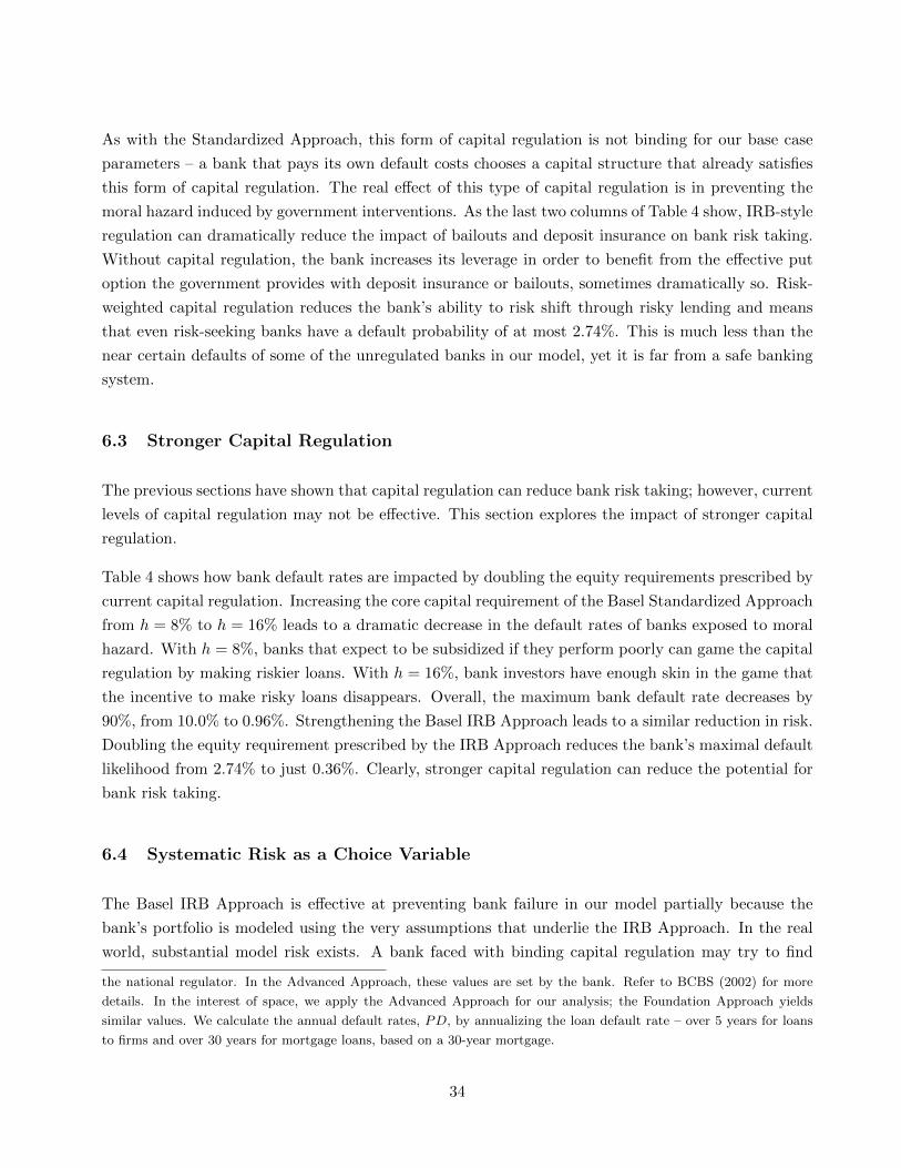
As with the Standardized Approach, this form of capital regulation is not binding for our base case

parameters – a bank that pays its own default costs chooses a capital structure that already satisfies

this form of capital regulation. The real effect of this type of capital regulation is in preventing the

moral hazard induced by government interventions. As the last two columns of Table 4 show, IRB-style

regulation can dramatically reduce the impact of bailouts and deposit insurance on bank risk taking.

Without capital regulation, the bank increases its leverage in order to benefit from the effective put

option the government provides with deposit insurance or bailouts, sometimes dramatically so. Risk-

weighted capital regulation reduces the bank’s ability to risk shift through risky lending and means

that even risk-seeking banks have a default probability of at most 2.74%. This is much less than the

near certain defaults of some of the unregulated banks in our model, yet it is far from a safe banking

system.

6.3 Stronger Capital Regulation

The previous sections have shown that capital regulation can reduce bank risk taking; however, current

levels of capital regulation may not be effective. This section explores the impact of stronger capital

regulation.

Table 4 shows how bank default rates are impacted by doubling the equity requirements prescribed by

current capital regulation. Increasing the core capital requirement of the Basel Standardized Approach

from h = 8% to h = 16% leads to a dramatic decrease in the default rates of banks exposed to moral

hazard. With h = 8%, banks that expect to be subsidized if they perform poorly can game the capital

regulation by making riskier loans. With h = 16%, bank investors have enough skin in the game that

the incentive to make risky loans disappears. Overall, the maximum bank default rate decreases by

90%, from 10.0% to 0.96%. Strengthening the Basel IRB Approach leads to a similar reduction in risk.

Doubling the equity requirement prescribed by the IRB Approach reduces the bank’s maximal default

likelihood from 2.74% to just 0.36%. Clearly, stronger capital regulation can reduce the potential for

bank risk taking.

6.4 Systematic Risk as a Choice Variable

The Basel IRB Approach is effective at preventing bank failure in our model partially because the

bank’s portfolio is modeled using the very assumptions that underlie the IRB Approach. In the real

world, substantial model risk exists. A bank faced with binding capital regulation may try to find

the national regulator. In the Advanced Approach, these values are set by the bank. Refer to BCBS (2002) for more

details. In the interest of space, we apply the Advanced Approach for our analysis; the Foundation Approach yields

similar values. We calculate the annual default rates, PD, by annualizing the loan default rate – over 5 years for loans

to firms and over 30 years for mortgage loans, based on a 30-year mortgage.

34

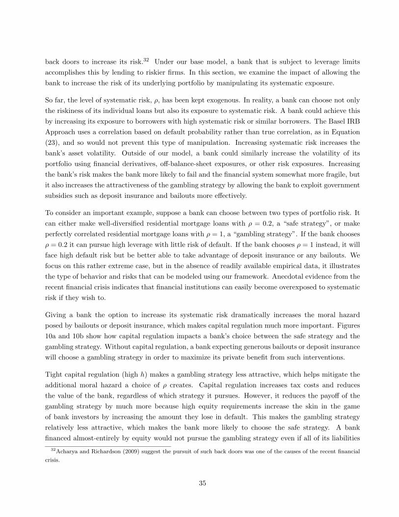
back doors to increase its risk.32 Under our base model, a bank that is subject to leverage limits

accomplishes this by lending to riskier firms. In this section, we examine the impact of allowing the

bank to increase the risk of its underlying portfolio by manipulating its systematic exposure.

So far, the level of systematic risk, ρ, has been kept exogenous. In reality, a bank can choose not only

the riskiness of its individual loans but also its exposure to systematic risk. A bank could achieve this

by increasing its exposure to borrowers with high systematic risk or similar borrowers. The Basel IRB

Approach uses a correlation based on default probability rather than true correlation, as in Equation

(23), and so would not prevent this type of manipulation. Increasing systematic risk increases the

bank’s asset volatility. Outside of our model, a bank could similarly increase the volatility of its

portfolio using financial derivatives, off-balance-sheet exposures, or other risk exposures. Increasing

the bank’s risk makes the bank more likely to fail and the financial system somewhat more fragile, but

it also increases the attractiveness of the gambling strategy by allowing the bank to exploit government

subsidies such as deposit insurance and bailouts more effectively.

To consider an important example, suppose a bank can choose between two types of portfolio risk. It

can either make well-diversified residential mortgage loans with ρ = 0.2, a “safe strategy”, or make

perfectly correlated residential mortgage loans with ρ = 1, a “gambling strategy”. If the bank chooses

ρ = 0.2 it can pursue high leverage with little risk of default. If the bank chooses ρ = 1 instead, it will

face high default risk but be better able to take advantage of deposit insurance or any bailouts. We

focus on this rather extreme case, but in the absence of readily available empirical data, it illustrates

the type of behavior and risks that can be modeled using our framework. Anecdotal evidence from the

recent financial crisis indicates that financial institutions can easily become overexposed to systematic

risk if they wish to.

Giving a bank the option to increase its systematic risk dramatically increases the moral hazard

posed by bailouts or deposit insurance, which makes capital regulation much more important. Figures

10a and 10b show how capital regulation impacts a bank’s choice between the safe strategy and the

gambling strategy. Without capital regulation, a bank expecting generous bailouts or deposit insurance

will choose a gambling strategy in order to maximize its private benefit from such interventions.

Tight capital regulation (high h) makes a gambling strategy less attractive, which helps mitigate the

additional moral hazard a choice of ρ creates. Capital regulation increases tax costs and reduces

the value of the bank, regardless of which strategy it pursues. However, it reduces the payoff of the

gambling strategy by much more because high equity requirements increase the skin in the game

of bank investors by increasing the amount they lose in default. This makes the gambling strategy

relatively less attractive, which makes the bank more likely to choose the safe strategy. A bank

financed almost-entirely by equity would not pursue the gambling strategy even if all of its liabilities

32Acharya and Richardson (2009) suggest the pursuit of such back doors was one of the causes of the recent financial

crisis.

35

were insured. Easing capital regulation means banks pursue the gambling strategy more often. In the

extreme, when there is no capital regulation, a bank chooses the gambling strategy if more than 74%

of its liabilities are insured deposits or it has a 18% chance of receiving a debt guarantee in the event

of failure.

An equity capital requirement of h = 8%, as in our model of the Basel Standardized Approach, means

that the bank gambles if insured deposits make up more than 84% of liabilities or the chance of a

bank debt guarantee is greater than 34%. Given that the average level of deposit insurance is well

above that and there is arguably a high chance of government bailouts, current capital regulation

may be insufficient, at least to the extent that banks can manipulate their risk. Figure 10 shows that

strengthening capital regulation in this manner curbs a bank’s incentive to gamble. Unreported, we get

similar results when we implement the same approach using the Vasicek-style IRB capital regulation.

Beyond the level of capital regulation, Figure 10 shows that moral hazard increases with the degree of

bailouts and deposit insurance. To prevent misbehavior, a bank that faces higher moral hazard needs

tighter capital regulation. In particular, banks funded primarily with insured deposits and banks that

are too-big-too-fail need stricter regulation. These banks have stronger incentives to misbehave, and

capital regulation that takes this into account could increase efficiency. Basel III includes additional

capital requirements for systemically important financial institutions, and we suggest that subjecting

banks funded primarily by deposits to similar regulation may improve efficiency.33

6.5 Cost of Capital Regulation

Capital regulation can substantially reduce moral hazard; however, any restriction on bank financial

structure may increase the interest rates banks charge to borrowers. Note that in our model these

high interest rates are not inefficient as they simply reflect less tax avoidance by banks. In a fuller

model, higher interest rates could translate into less investment or other forms of inefficiency.

We find that capital regulation slightly increases the interest rates paid by borrower firms: Increasing

equity capital requirements by one percentage point increases firm interest rates by half of one basis

point, as illustrated in Figure 11. This estimate is in line with the empirical results of Kisin and

Manela (2013) and the theoretical results of Kashyap, Stein, and Hanson (2010). This estimate is

almost an order of magnitude lower than that of the BCBS (2010) which assumes that a bank’s return

on equity is fixed and exogenous.34

33Refer to the BCBS (2011) for more detail on the additional capital requirements for systemically important financial

institutions.34Such an approach ignores the fundamental effects of bank leverage on the cost of equity as implied by Modigliani and

Miller (1958). Admati, DeMarzo, Hellwig, and Pfleiderer (2013a) and Admati and Hellwig (2013) provide an extensive

discussion of this error in the context of bank regulation.

36

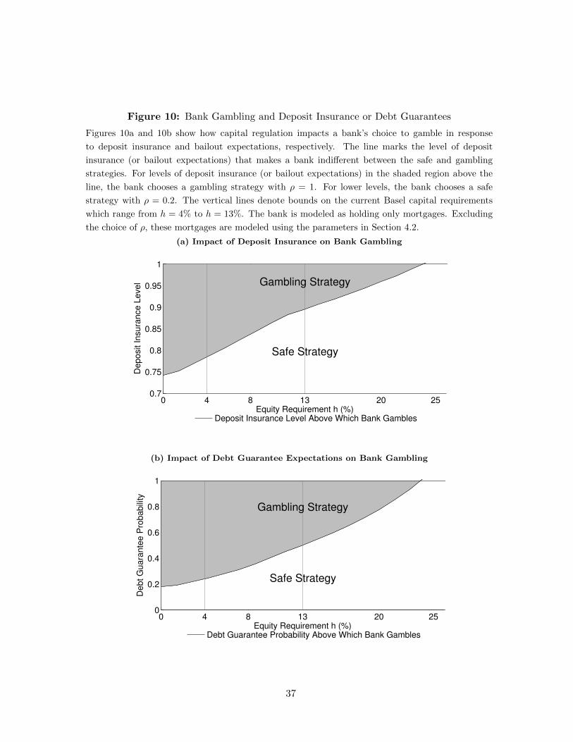
Figure 10: Bank Gambling and Deposit Insurance or Debt Guarantees

Figures 10a and 10b show how capital regulation impacts a bank’s choice to gamble in response

to deposit insurance and bailout expectations, respectively. The line marks the level of deposit

insurance (or bailout expectations) that makes a bank indifferent between the safe and gambling

strategies. For levels of deposit insurance (or bailout expectations) in the shaded region above the

line, the bank chooses a gambling strategy with ρ = 1. For lower levels, the bank chooses a safe

strategy with ρ = 0.2. The vertical lines denote bounds on the current Basel capital requirements

which range from h = 4% to h = 13%. The bank is modeled as holding only mortgages. Excluding

the choice of ρ, these mortgages are modeled using the parameters in Section 4.2.

(a) Impact of Deposit Insurance on Bank Gambling

0 4 8 13 20 250.7

0.75

0.8

0.85

0.9

0.95

1

Equity Requirement h (%)

Deposit Insura

nce L

evel

Gambling Strategy

Safe Strategy

Deposit Insurance Level Above Which Bank Gambles

(b) Impact of Debt Guarantee Expectations on Bank Gambling

0 4 8 13 20 250

0.2

0.4

0.6

0.8

1

Equity Requirement h (%)

Debt G

uara

nte

e P

robabili

ty

Gambling Strategy

Safe Strategy

Debt Guarantee Probability Above Which Bank Gambles

37

Figure 11: Impact of Capital Regulation on Mortgage Interest Rates

Figure 11 shows how capital regulation impacts the interest rates on mortgage loans. The vertical

lines denote bounds on the current Basel capital requirements which range from h = 4% to h = 13%.

The bank is modeled as holding only mortgages. These mortgages are modeled using the parameters

in Section 4.2.

0 4 8 13 20 30 40 504

4.2

4.4

4.6

4.8

5

Mort

gage Inte

rst R

ate

(%

)

Equity Requirement h (%)

This cost is numerically small. However, our partial equilibrium framework does not consider all

of the costs and benefits of regulation and so we can make only cautious statements on the welfare

implications of capital regulation. Notably, we only consider the private costs of bank failure. The

social costs of a failed bank may be much greater and including these costs would increase the value of

capital regulation. Neither the bank’s capital structure decision nor the interest rates it charges take

into account such externalities.

If regulators want banks to reduce leverage and risk, eliminating the distortions created by the tax

benefit of debt may be simpler and more important than reforming deposit insurance or the too-big-

to-fail dimension of banks. These are inherently private benefits as they are a transfer from taxpayers

to private agents. Thus, eliminating the tax deductibility of interest, or equalizing the tax treatment

of debt and equity in some other way, would remove all the wasteful distortions we consider.

7 Extensions

In this section, we briefly discuss a number of extensions of our framework. First, we consider alterna-

tive mechanisms for debt benefits, other than taxes. Second, we introduce imperfect bank competition

and analyze the consequences of bank bargaining power. Third, we analyze the introduction of bond

markets that compete with banks in the corporate loan market. The upshot is that the main results,

38

both qualitative and quantitative, remain robust to these extensions. For brevity, we mention only

the main results of these extensions. The online appendix provides details.

Alternative Debt Benefits. Tax benefits drive the debt decisions of banks and firms in the preceding

sections. Appendix A considers other debt benefits. Namely, we consider a DeAngelo and Stulz (2013)

style liquidity provision benefit and a Baker and Wurgler (2013) style reduced discount rate for debt.

Replacing the tax benefit of debt with either of these frictions produces similar results. Again, we

see banks with high leverage because, as explained in Section 3, even a small benefit to debt will

cause banks to pursue high leverage. Applying the aforementioned frictions, we see bank leverage that

ranges from 83% to 100%.

Bank Bargaining Power. The previous sections use zero profit banks for simplicity; however, this

assumption can easily be relaxed. Appendix B explores the effect of exogenously varying the spread

banks charge. We see that increasing bank bargaining power also increases bank leverage. Banks that

are more profitable pay tax in more states of the world and get greater tax benefits from debt issuance.

This means our zero profit assumption leads us to slightly underestimate bank leverage.

Bond Markets. Appendix C adds junior bond holders to our model of financing. Adding junior

bond holders means that banks are more senior. This reduces the riskiness of bank portfolios and

allows banks to pursue even higher leverage. Firm leverage increases as firm borrowing now imposes

less systemic risk on banks. Bank leverage also increases, although only slightly, as corporate debt

makes up only a small part of the bank’s portfolio.

8 What Is Missing?

Perhaps the greatest advantage of our framework is that policy makers, practitioners, and academics

alike can use it to quantify the impact of various regulatory measures on both the financial and real

sectors of the economy. Thus, it is important to mention several extensions that would add further

realism to our framework, but are outside the scope of this paper.

Our model uses constant and commonly known parameters; however, Bhamra, Kuehn, and Strebulaev

(2010) and others have shown that the time variation of parameters can be crucial, especially variation

of those parameters related to macroeconomic risk. For example, if volatility unexpectedly increases,

the incentives of firms and banks change and the effectiveness of time-invariant capital regulation

deteriorates. Considering such parameter variation would be an important extension. In addition,

most parameters are imperfectly known and are learned over time by market participants (including

firms and banks). Our model could be extended to explore the impact of this learning on financial

decisions and systemic fragility.

39

We model the borrowing firms and households as ex-ante homogenous. Realistically, banks deal with

heterogeneous borrowers and the distribution of borrower leverage may have a non-trivial impact on

our results. Modeling firm investment decisions more directly would add a further layer of richness.

Finally, we have considered only the private costs and benefits of defaults, interventions, and taxes.

The externalities imposed by bank failure, particularly systemic bank failure, are more important

considerations when setting policy. A more detailed analysis could extend our framework to multiple

banks in order to examine how bank incentives impact systemic risk.

9 Conclusion

In this paper, we propose a novel framework to model the joint debt decisions of banks and their

borrowers. This framework combines a model bank regulators use to assess risk with a model academics

use to explain capital structure. Our structure can be used to explore the quantitative impact of

government interventions such as deposit insurance, bailouts, and capital regulation.

Banks are diversified senior creditors, which reduces their risk and allows them to take on high lever-

age. The bank’s borrowers respond to this high leverage by reducing own their borrowing, partially

explaining low corporate leverage. Our benchmark parameters give rise to banks with leverage of 87%

and firms with leverage of 30%, not dissimilar to what we observe empirically.

Banks funded primarily with insured deposits or banks that are likely to be bailed out face strong

incentives to take on risk. We quantify these effects and find that moderate levels of deposit insurance

or small probabilities of bailouts increase bank risk taking only marginally. However, larger interven-

tions create extreme moral hazard that can push banks into a risk-seeking strategy. Many banks have

enough insured deposits to face such extreme moral hazard.

Strong, targeted capital regulation combats this moral hazard and reduces bank failure. The proposed

Basel III capital requirements may be insufficient for banks that are too-big-to-fail or have large

amounts of insured deposits, especially if banks can manipulate loan characteristics. Increasing capital

requirements to 16% significantly reduces bank risk and only slightly increases borrowing costs. We

calculate that increasing bank equity requirement by 1% increases borrower cost by only half of a basis

point, suggesting that capital regulation could be substantially strengthened.

Obviously, we have just scratched the surface of these issues. Regulators, academics, and practitioners

continue to have a discussion on bank capital structure, systemic risk, and capital regulation. The

framework we present is rich and flexible enough to address many of their unanswered questions.

40

References

Acharya, Viral, Hamid Mehran, Til Schuermann, and Anjan Thakor, 2011, Robust capital regulation,

Discussion paper, Staff Report, Federal Reserve Bank of New York.

Acharya, Viral, Hamid Mehran, and Anjan Thakor, 2013, Caught between scylla and charybdis?

regulating bank leverage when there is rent-seeking and risk-shifting, Manuscript.

Acharya, Viral V., Sreedhar T. Bharath, and Anand Srinivasan, 2007, Does industry-wide distress

affect defaulted firms? Evidence from creditor recoveries, Journal of Financial Economics 85, 787–

821.

Acharya, Viral V., and Matthew Richardson, 2009, Causes of the financial crisis, Critical Review 21,

195–210.

Admati, Anat R., Peter M. DeMarzo, Martin F. Hellwig, and Paul Pfleiderer, 2013a, Fallacies, ir-

relevant facts, and myths in the discussion of capital regulation: Why bank equity is not socially

expensive, Working Paper, Stanford University.

, 2013b, The leverage ratchet effect, Working Paper, Stanford University.

Admati, Anat R., and Martin F. Hellwig, 2013, The Bankers’ New Clothes (Princeton University

Press).

Adrian, Tobias, and Hyun Song Shin, 2010, Liquidity and leverage, Journal of Financial Intermedia-

tion 19, 418–437.

Allen, Franklin, and Elena Carletti, 2013, Deposits and bank capital structure, Working Paper, Uni-

versity of Pennsylvania.

Amromin, Gene, and Anna Paulson, 2010, Default rates on prime and subprime mortgages: Differences

& similarities, Profitwise News and Views.

Baker, Malcolm, and Jeffrey Wurgler, 2013, Do strict capital requirements raise the cost of capital?

Banking regulation and the low risk anomaly, Discussion paper, National Bureau of Economic

Research.

Basel Committee on Banking Supervision, 2002, Quantitative impact study 3: Technical guidance,

Bank for International Settlements.

, 2004, Basel II: International convergence of capital measurement and capital standards: A

revised framework, Bank for International Settlements.

, 2010, An assessment of the long-term economic impact of stronger capital and liquidity

requirements, Bank for International Settlements.

41

, 2011, Basel III: A global regulatory framework for more resilient banks and banking systems,

Bank for International Settlements.

, 2013, Global systemically important banks: Updated assessment methodology and the higher

loss absorbency requirement, Bank for International Settlements.

Berger, Allen N., and Christa H.S. Bouwman, 2013, How does capital affect bank performance during

financial crises?, Journal of Financial Economics 109, 146–176.

Berger, Allen N., Robert DeYoung, Mark J. Flannery, David Lee, and Ozde Oztekin, 2008, How do

large banking organizations manage their capital ratios?, Journal of Financial Services Research

34, 123–149.

Bhamra, Harjoat S., Lars-Alexander Kuehn, and Ilya A. Strebulaev, 2010, The aggregate dynamics

of capital structure and macroeconomic risk, Review of Financial Studies 23, 4187–4241.

Bhattacharya, Sugato, and Amiyatosh Purnanandam, 2011, Risk-taking by banks: What did we know

and when did we know it?, Manuscript.

Bokhari, Sheharyar, Walter Torous, and William Wheaton, 2013, Why did household mortgage lever-

age rise from the mid-1980s until the great recession?, Working Paper, Massachusetts Institute of

Technology.

Bruno, Valentina, and Hyun Song Shin, 2013, Capital flows, cross-border banking and global liquidity,

Manuscript.

Bullard, James, 2012, The aftermath of the housing bubble, Speech, Federal Reserve Bank of St. Louis.

Bulow, Jeremy, and Paul Klemperer, 2013, Market-based bank capital regulation, Manuscript.

Campbell, John Y, and Joao F Cocco, 2011, A model of mortgage default, Discussion paper, National

Bureau of Economic Research.

Choi, Jaewon, and Matthew Richardson, 2008, The volatility of firm’s assets and the leverage effect,

AFA 2010 Atlanta Meetings Paper.

Congressional Budget Office, 2010, Fannie Mae, Freddie Mac, and the federal role in the secondary

mortgage market, Washington D.C.

Cotter, John, Stuart Gabriel, and Richard Roll, 2011, Integration and contagion in US housing mar-

kets, Working Paper, UCLA.

Davydenko, Sergei, Ilya A. Strebulaev, and Xiaofei Zhao, 2012, A market-based study of the cost of

default, Review of Financial Studies 25, 2959–2999.

42

DeAngelo, Harry, and Ronald W. Masulis, 1980, Optimal capital structure under corporate and per-

sonal taxation, Journal of Financial Economics 8, 3–29.

DeAngelo, Harry, and Rene M. Stulz, 2013, Why high leverage is optimal for banks, Working Paper,

University of Southern California.

Diamond, Douglas W., 1984, Financial intermediation and delegated monitoring, The Review of Eco-

nomic Studies 51, 393–414.

, and Philip H. Dybvig, 1983, Bank runs, deposit insurance, and liquidity, Journal of Political

Economy 91, 401–19.

Diamond, Douglas W., and Raghuram G. Rajan, 2000, A theory of bank capital, Journal of Finance

55, 2431–2465.

Dietsch, Michel, and Joel Petey, 2004, Should SME exposures be treated as retail or corporate expo-

sures? A comparative analysis of default probabilities and asset correlations in French and German

SMEs, Journal of Banking & Finance 28, 773–788.

Elliott, Douglas, Suzanne Salloy, and Andre Santos, 2012, Assessing the cost of financial regulation,

IMF Working Paper.

Faulkender, Michael, and Rong Wang, 2006, Corporate financial policy and the value of cash, Journal

of Finance 61, 1957–1990.

Glover, Brent, 2012, The expected cost of default, Working Paper, Carnegie Mellon University.

Goldstein, Robert, Nengjiu Ju, and Hayne Leland, 2001, An EBIT-based model of dynamic capital

structure, Journal of Business 74, 483–512.

Graham, John R., 1996, Debt and the marginal tax rate, Journal of Financial Economics 41, 41–73.

, 2000, How big are the tax benefits of debt?, Journal of Finance 55, 1901–1941.

, and Alan L. Tucker, 2006, Tax shelters and corporate debt policy, Journal of Financial

Economics 81, 563–594.

Hanson, Samuel G., Anil K. Kashyap, and Jeremy C. Stein, 2011, A macroprudential approach to

financial regulation, Journal of Economic Perspectives 25, 3–28.

Harding, John, Xiaozhong Liang, and Stephen Ross, 2006, The optimal capital structure of banks

under deposit insurance and capital requirements, Manuscript.

Harding, John P., Xiaozhing Liang, and Stephen L. Ross, 2007, The optimal capital structure of

banks: Balancing deposit insurance, capital requirements and tax-advantaged debt, Working Paper,

University of Connecticut.

43

Harris, Milton, Christian C. Opp, and Marcus M. Opp, 2014, Macroprudential bank capital regulation:

Local vs. global optima, Working Paper, University of Chicago.

Hassan, M. Kabir, Gordon V. Karels, and Manfred O. Peterson, 1994, Deposit insurance, market

discipline and off-balance sheet banking risk of large U.S. commercial banks, Journal of Banking &

Finance 18, 575–593.

International Monetary Fund, 2008, Global financial stability report, Washington D.C.

James, Christopher, 1991, The losses realized in bank failures, Journal of Finance 46, 1223–1242.

Ju, Nengjiu, Robert Parrino, Allen M. Poteshman, and Michael S. Weisbach, 2005, Horses and rabbits?

Trade-off theory and optimal capital structure, Journal of Financial and Quantitative Analysis 40,

259–281.

Kashyap, Anil K, Jeremy C Stein, and Samuel Hanson, 2010, An analysis of the impact of substan-

tially heightened capital requirements on large financial institutions, Working Paper, University of

Chicago.

Kisin, Roni, and Asaf Manela, 2013, The shadow cost of bank capital requirements, Working Paper,

Washington University in St. Louis.

Krainer, John, and Stephen LeRoy, 2010, Underwater mortgages, FRBSF Economic Letter.

Kraus, Alan, and Robert H. Litzenberger, 1973, A state-preference model of optimal financial leverage,

Journal of Finance 28, 911–922.

Lambert, Claudia, Felix Noth, and Ulrich Schuwer, 2012, How do banks react to increased asset risks?

Evidence from Hurricane Katrina, 29th International Conference of the French Finance Association

(AFFI).

Le Lesle, Vanessa, and Sofiya Avramova, 2012, Revisiting risk-weighted assets, IMF Working Paper.

Leland, Hayne E., 1994, Corporate debt value, bond covenants, and optimal capital structure, Journal

of Finance 49, 1213–1252.

, 1998, Agency costs, risk management, and capital structure, Journal of Finance 53, 1213–

1243.

Lopez, Jose A., 2004, The empirical relationship between average asset correlation, firm probability

of default, and asset size, Journal of Financial Intermediation 13, 265–283.

Merton, Robert C., 1974, On the pricing of corporate debt: The risk structure of interest rates, Journal

of Finance 29, 449–470.

Miller, Merton H., 1977, Debt and taxes, Journal of Finance 32, 261–275.

44

Modica, Giuseppe, and Laura Poggiolini, 2012, A First Course in Probability and Markov Chains

(Wiley).

Modigliani, Franco, and Merton H. Miller, 1958, The cost of capital, corporation finance and the

theory of investment, American Economic Review 48, 261–297.

Morellec, Erwan, 2004, Can managerial discretion explain observed leverage ratios?, Review of Finan-

cial Studies 17, 257–294.

Neave, Charles, and Gilbert M. Grosvenor, 1954, Helping Holland rebuild her land: American students

lend a hand as the gallant Dutch repair the ravages of their country’s old enemy, the sea, National

Geographic Magazine CVI, 99–47.

Office of the Comptroller of the Currency and the Board of Governors of the Federal Reserve System,

2013, Basel III implementation: Final rule, Department of the Treasury and the Federal Reserve

System.

Ou, S., D. Chlu, and A. Metz, 2011, Corporate default and recovery rates, 1920–2010, Special Com-

ment, Moodys Investors Service.

Qi, Min, and Xiaolong Yang, 2009, Loss given default of high loan-to-value residential mortgages,

Journal of Banking & Finance 33, 788–799.

Roberts, Michael R., and Amir Sufi, 2009, Renegotiation of financial contracts: Evidence from private

credit agreements, Journal of Financial Economics 93, 159–184.

Ronn, Ehud I., and Avinash K. Verma, 1986, Pricing risk-adjusted deposit insurance: An option-based

model, Journal of Finance 41, 871–896.

Schaefer, Stephen M., and Ilya A. Strebulaev, 2008, Structural models of credit risk are useful: Evi-

dence from hedge ratios on corporate bonds, Journal of Financial Economics 90, 1–19.

Schandlbauer, Alexander, 2013, How do financial institutions react to a tax increase, Manuscript.

Schepens, Glenn, 2013, Taxes and bank capital structure, Manuscript.

Strebulaev, Ilya A., 2007, Do tests of capital structure theory mean what they say?, Journal of Finance

62, 1747–1787.

, and Baozhong Yang, 2013, The mystery of zero-leverage firms, Journal of Financial Eco-

nomics 109, 1–23.

Thakor, Anjan V., 2013, Bank capital and financial stability: An economic tradeoff or a faustian

bargain?, Manuscript.

Vasicek, Oldrich, 2002, The distribution of loan portfolio value, Risk 15, 160–162.

45

Westerback, Diane, Keitaro Okuyama, Vidhya Venkatachalam, Abhishek Tiwary, Ted Burbage, and

Ernestine Warner, 2011, U.S. residential mortgage performance index, Standard & Poor’s.

Zhou, Yu, and Donald R Haurin, 2010, On the determinants of house value volatility, Journal of Real

Estate Research 32, 377–395.

46

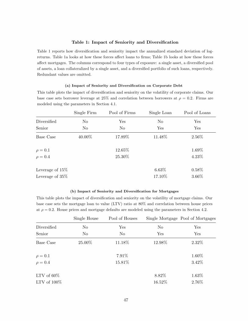
Table 1: Impact of Seniority and Diversification

Table 1 reports how diversification and seniority impact the annualized standard deviation of log-

returns. Table 1a looks at how these forces affect loans to firms; Table 1b looks at how these forces

affect mortgages. The columns correspond to four types of exposure: a single asset, a diversified pool

of assets, a loan collateralized by a single asset, and a diversified portfolio of such loans, respectively.

Redundant values are omitted.

(a) Impact of Seniority and Diversification on Corporate Debt

This table plots the impact of diversification and seniority on the volatility of corporate claims. Our

base case sets borrower leverage at 25% and correlation between borrowers at ρ = 0.2. Firms are

modeled using the parameters in Section 4.1.

Single Firm Pool of Firms Single Loan Pool of Loans

Diversified No Yes No Yes

Senior No No Yes Yes

Base Case 40.00% 17.89% 11.48% 2.56%

ρ = 0.1 12.65% 1.69%

ρ = 0.4 25.30% 4.23%

Leverage of 15% 6.63% 0.58%

Leverage of 35% 17.10% 3.66%

(b) Impact of Seniority and Diversification for Mortgages

This table plots the impact of diversification and seniority on the volatility of mortgage claims. Our

base case sets the mortgage loan to value (LTV) ratio at 80% and correlation between house prices

at ρ = 0.2. House prices and mortgage defaults are modeled using the parameters in Section 4.2.

Single House Pool of Houses Single Mortgage Pool of Mortgages

Diversified No Yes No Yes

Senior No No Yes Yes

Base Case 25.00% 11.18% 12.98% 2.32%

ρ = 0.1 7.91% 1.60%

ρ = 0.4 15.81% 3.42%

LTV of 60% 8.82% 1.63%

LTV of 100% 16.52% 2.76%

47

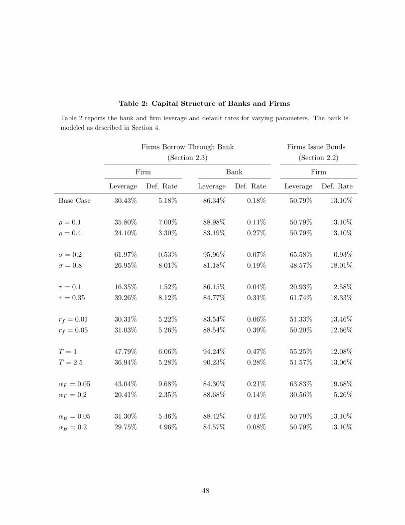
Table 2: Capital Structure of Banks and Firms

Table 2 reports the bank and firm leverage and default rates for varying parameters. The bank is

modeled as described in Section 4.

Firms Borrow Through Bank Firms Issue Bonds

(Section 2.3) (Section 2.2)

Firm Bank Firm

Leverage Def. Rate Leverage Def. Rate Leverage Def. Rate

Base Case 30.43% 5.18% 86.34% 0.18% 50.79% 13.10%

ρ = 0.1 35.80% 7.00% 88.98% 0.11% 50.79% 13.10%

ρ = 0.4 24.10% 3.30% 83.19% 0.27% 50.79% 13.10%

σ = 0.2 61.97% 0.53% 95.96% 0.07% 65.58% 0.93%

σ = 0.8 26.95% 8.01% 81.18% 0.19% 48.57% 18.01%

τ = 0.1 16.35% 1.52% 86.15% 0.04% 20.93% 2.58%

τ = 0.35 39.26% 8.12% 84.77% 0.31% 61.74% 18.33%

rf = 0.01 30.31% 5.22% 83.54% 0.06% 51.33% 13.46%

rf = 0.05 31.03% 5.26% 88.54% 0.39% 50.20% 12.66%

T = 1 47.79% 6.06% 94.24% 0.47% 55.25% 12.08%

T = 2.5 36.94% 5.28% 90.23% 0.28% 51.57% 13.06%

αF = 0.05 43.04% 9.68% 84.30% 0.21% 63.83% 19.68%

αF = 0.2 20.41% 2.35% 88.68% 0.14% 30.56% 5.26%

αB = 0.05 31.30% 5.46% 88.42% 0.41% 50.79% 13.10%

αB = 0.2 29.75% 4.96% 84.57% 0.08% 50.79% 13.10%

48

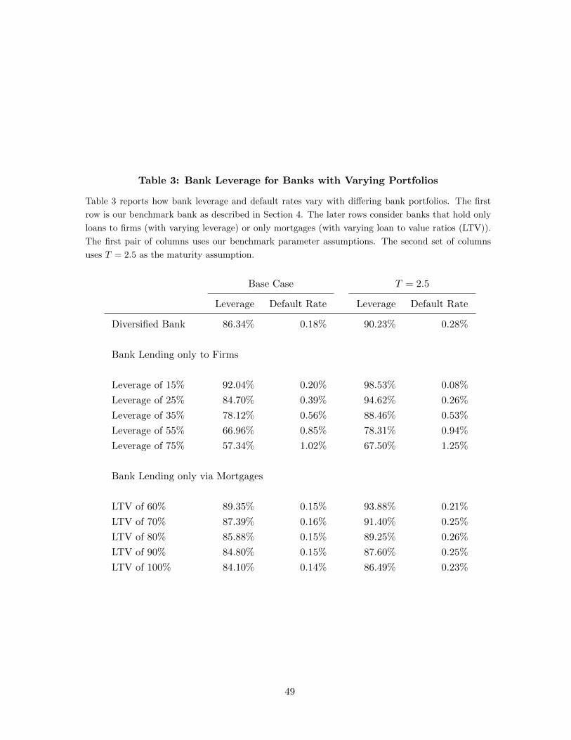
Table 3: Bank Leverage for Banks with Varying Portfolios

Table 3 reports how bank leverage and default rates vary with differing bank portfolios. The first

row is our benchmark bank as described in Section 4. The later rows consider banks that hold only

loans to firms (with varying leverage) or only mortgages (with varying loan to value ratios (LTV)).

The first pair of columns uses our benchmark parameter assumptions. The second set of columns

uses T = 2.5 as the maturity assumption.

Base Case T = 2.5

Leverage Default Rate Leverage Default Rate

Diversified Bank 86.34% 0.18% 90.23% 0.28%

Bank Lending only to Firms

Leverage of 15% 92.04% 0.20% 98.53% 0.08%

Leverage of 25% 84.70% 0.39% 94.62% 0.26%

Leverage of 35% 78.12% 0.56% 88.46% 0.53%

Leverage of 55% 66.96% 0.85% 78.31% 0.94%

Leverage of 75% 57.34% 1.02% 67.50% 1.25%

Bank Lending only via Mortgages

LTV of 60% 89.35% 0.15% 93.88% 0.21%

LTV of 70% 87.39% 0.16% 91.40% 0.25%

LTV of 80% 85.88% 0.15% 89.25% 0.26%

LTV of 90% 84.80% 0.15% 87.60% 0.25%

LTV of 100% 84.10% 0.14% 86.49% 0.23%

49

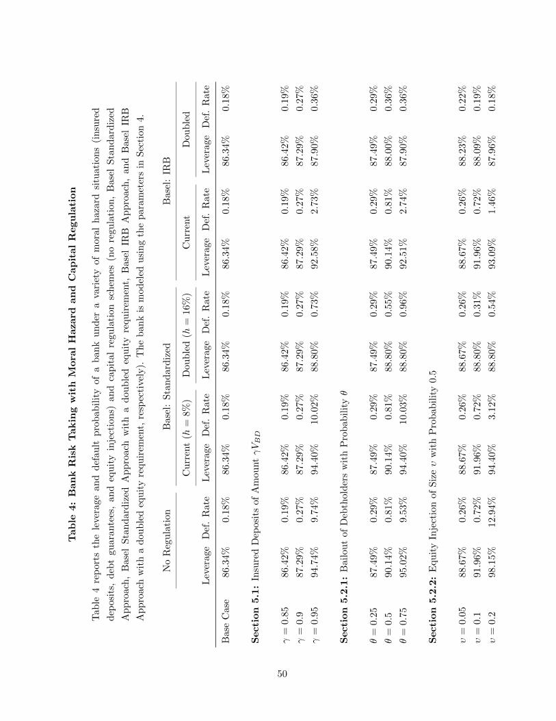
Tab

le4:

Ban

kR

isk

Takin

gw

ith

Mora

lH

azard

an

dC

ap

ital

Regu

lati

on

Tab

le4

rep

ort

sth

ele

vera

gean

dd

efau

ltp

rob

abil

ity

ofa

ban

ku

nd

era

vari

ety

ofm

ora

lh

aza

rdsi

tuati

on

s(i

nsu

red

dep

osi

ts,

deb

tgu

ara

nte

es,

an

deq

uit

yin

ject

ions)

and

cap

ital

regu

lati

onsc

hem

es(n

ore

gu

lati

on

,B

ase

lS

tan

dard

ized

Ap

pro

ach

,B

asel

Sta

nd

ard

ized

Ap

pro

ach

wit

ha

dou

ble

deq

uit

yre

qu

irem

ent,

Bas

elIR

BA

pp

roach

,an

dB

ase

lIR

B

Ap

pro

ach

wit

ha

dou

ble

deq

uit

yre

qu

irem

ent,

resp

ecti

vely

).T

he

ban

kis

mod

eled

usi

ng

the

para

met

ers

inS

ecti

on

4.

No

Reg

ula

tion

Bas

el:

Sta

nd

ard

ized

Base

l:IR

B

Cu

rren

t(h

=8%

)D

oub

led

(h=

16%

)C

urr

ent

Dou

ble

d

Lev

erag

eD

ef.

Rat

eL

ever

age

Def

.R

ate

Lev

erag

eD

ef.

Rat

eL

ever

age

Def

.R

ate

Lev

erage

Def

.R

ate

Bas

eC

ase

86.3

4%

0.18%

86.

34%

0.18

%86

.34%

0.18

%86

.34%

0.1

8%

86.3

4%

0.1

8%

Secti

on

5.1

:In

sure

dD

eposi

tsof

Am

ou

ntγVBD

γ=

0.85

86.4

2%

0.19%

86.

42%

0.19

%86

.42%

0.19

%86

.42%

0.1

9%

86.4

2%

0.1

9%

γ=

0.9

87.2

9%

0.27%

87.

29%

0.27

%87

.29%

0.27

%87

.29%

0.2

7%

87.2

9%

0.2

7%

γ=

0.95

94.7

4%

9.74%

94.

40%

10.0

2%88

.80%

0.73

%92

.58%

2.7

3%

87.9

0%

0.3

6%

Secti

on

5.2

.1:

Bai

lou

tof

Deb

thol

der

sw

ith

Pro

bab

ilit

yθ

θ=

0.25

87.

49%

0.2

9%

87.

49%

0.29

%87

.49%

0.29

%87

.49%

0.2

9%

87.4

9%

0.2

9%

θ=

0.5

90.1

4%

0.81%

90.1

4%0.

81%

88.8

0%0.

55%

90.1

4%

0.8

1%

88.0

0%

0.3

6%

θ=

0.75

95.

02%

9.5

3%

94.

40%

10.0

3%88

.80%

0.96

%92

.51%

2.7

4%

87.9

0%

0.3

6%

Secti

on

5.2

.2:

Equ

ity

Inje

ctio

nof

Siz

eυ

wit

hP

rob

abil

ity

0.5

υ=

0.05

88.

67%

0.2

6%

88.6

7%0.

26%

88.6

7%0.

26%

88.6

7%

0.2

6%

88.2

3%

0.2

2%

υ=

0.1

91.9

6%

0.72%

91.

96%

0.72

%88

.80%

0.31

%91

.96%

0.7

2%

88.0

9%

0.1

9%

υ=

0.2

98.1

5%

12.

94%

94.

40%

3.12

%88

.80%

0.54

%93

.09%

1.4

6%

87.9

6%

0.1

8%

50