Financiers vs. Engineers:Should the Financial Sector be Taxed or Subsidized?∗

Thomas Philippon†

New York University

October 2007

Abstract

I study the allocation of human capital in an economy with production externalities, fi-nancial constraints and career choices. Agents choose to become entrepreneurs, workersor financiers. Entrepreneurship has positive externalities, but innovators face borrow-ing constraints and require the services of financiers in order to invest efficiently. Wheninvestment and education subsidies are chosen optimally, I find that the financial sec-tor should be taxed in exactly the same way as the non-financial sector. When directsubsidies to investment and scientific education are not feasible, giving a preferred taxtreatment to the financial sector can improve welfare by increasing aggregate investmentin research and development.

∗I thank Holger Mueller, and seminar participants at the Paris School of Economics and CREI-UniversitatPompeu Fabra for their comments.

†Stern School of Business, NBER and CEPR.

1

This paper studies optimal financial development by analyzing the interactions between

the financial and non-financial sectors. On the one hand, entrepreneurs need financial

services to overcome problems of moral hazard and adverse selection. An efficient finan-

cial sector is therefore critical for economic growth. On the other hand, the financial and

non-financial sectors compete for the same scarce supply of human capital. Without ex-

ternalities, the competitive allocation is optimal. In many innovative activities, however,

social returns exceed private returns. Does this lead to an inefficient allocation of human

capital? If so, are there too many or too few financiers? What kind of corrective taxes

should be implemented?

I study these questions by combining insights from the endogenous growth and financial

development literatures. External effects play an important role in the analysis of Romer

(1986) and Lucas (1988). Moreover, in most models of endogenous growth, the decen-

tralization of the Pareto optimum requires subsidizing investment, production or R&D, as

discussed in Aghion and Howitt (1998) and Barro and Sala-i-Martin (2004). The number

of entrepreneurs can be inefficiently low in the competitive equilibrium because social re-

turns to innovation exceed private returns. Indeed, Baumol (1990) and Murphy, Shleifer,

and Vishny (1991) argue that the flow of talented individuals into law and financial services

might not be entirely desirable, because social returns might be higher in other occupations,

even though private returns are not.

On the other hand, however, a large body of research has shown the importance of

efficient financial markets for economic growth. Levine (2005), in his comprehensive survey,

argues that “better functioning financial systems ease the external financing constraints

that impede firm and industrial expansion, suggesting that this is one mechanism through

which financial development matters for growth.”

These issues have become increasingly relevant over time, for several reasons. Immedi-

ately after World War II, the financial sector accounted for less than 2.5% of all labor income

in the United States. In 2007, this share is close to 8%. Moreover, since the early 1980s,

the growth of the financial sector has been strongly biased towards highly skilled individ-

uals (Philippon and Resheff (2007)). Some individuals, who would have become engineers

in the 1960s, now become financiers.1 The decline in engineering has prompted a debate

1“Thirty to forty percent of Duke Masters of Engineering Management students were accepting jobs

2

about the role of science and technology in U.S. economic performance. It is commonly

argued that policy interventions that promote science and technology are desirable because

of externalities in knowledge and the diffusion of new technologies (National Academy of

Sciences (2007)).2

This line of reasoning also appears in the debate about the tax treatment of hedge funds

and private equity funds. Hedge funds and private equity funds have their fees taxed at the

15 percent capital gains rate rather than the 35 percent ordinary income rate. The properties

of an optimal tax system are not a priori obvious. On the one hand, one could argue that

finance diverts resources from entrepreneurship and scientific progress. For instance, critics

of the finance industry argue that lower taxes for private equity firms and fund managers

distort the incentives of college students when they decide what career to pursue.3 On the

other hand, executives of investment funds argue that they promote economic growth by

relaxing entrepreneurs’ constraints, which justifies their preferred tax treatment.

I propose a simple model where one can evaluate the relative merits of these seemingly

contradictory arguments. In the model, agents choose to become workers, entrepreneurs

or financiers. Like in the endogenous growth literature, entrepreneurs have the ability to

innovate, and these innovations have positive externalities. Like in the financial development

literature, innovators face binding borrowing constraints and may require the use of financial

services in order to invest efficiently. I characterize the social planner’s allocation and the

competitive equilibrium, and I study the efficiency of various tax systems.

I obtain the following results. First of all, the model makes it clear that one should

not discuss optimal taxation without taking into account direct subsidies to investment,

R&D or scientific education. More precisely, I show that the constrained efficient allocation

can always be decentralized with the same tax rate on income in the financial and non-

financial sectors. The constrained efficient allocation requires just an investment subsidy

when the external effects depend only on aggregate investment, as in Romer (1986). When

outside of the engineering profession. They chose to become investment bankers or management consultantsrather than engineers.” Vivek Wadhwa, Testimony to the U.S. House of Representatives, May 16, 2006.

2 “Our goal should be to double the number of science, technology, and mathematics graduates in theUnited States by 2015. This will require both funding and innovative ideas.” Bill Gates, Testimony to theU.S. Senate, March 7, 2007

3 “Industry Groups Warn of Adverse Effects of Private Equity Tax Hike”, Alan Zibel, Associated PressBusiness Writer, Tuesday July 31 2007. See in particualr the quotes of Joseph Bankman, law professor atStanford University, and Bruce Rosenblum, managing director of the Carlyle Group.

3

the external effects also depend directly on the number of entrepreneurs, the second best

requires positive subsidies to scientific education (or, equivalently, equal and positive tax

rates on workers and financiers).

In any case, the presence of binding credit constraints does not invalidate the prescription

that, whenever possible, externalities should be corrected at the source. The second-best

subsidies increase the incentives of agents to become entrepreneurs and to invest in research

and development. In equilibrium, the demand for labor and financial services adjust and

there is no reason to tax financiers more or less than workers. The fact that financial services

help relax borrowing constraints does not change this result.

Interestingly, the specificity of financing constraints and their impact on the optimal

taxation of the financial sector appear when one moves away from the second best. In

practice, and for a variety of reasons, governments are unlikely to be able to set the optimal

education and investment subsidies. Starting from a competitive equilibrium without cor-

rective taxation, a subsidy given to the financial sector could then enhance welfare. I show

that subsidizing the financial sector is generally useful if one seeks to increase aggregate

investment. If one is more interested in increasing the number of entrepreneurs, on the

other hand, it might be optimal to tax the financial sector.

The rest of the paper is organized as follows. Section 1 lays down the model and discusses

how it relates to the literature. Section 2 characterizes the social planner’s allocation. Sec-

tion 3 derives the competitive equilibrium outcome and compares it to the social planner’s

outcome. Section 4 shows how the second best allocation can be decentralized, and then

discusses optimal taxation in a third-best economy with limited tax instruments. Section 5

concludes.

1 The model

1.1 Technology and preferences

Consider an economy with overlapping generations. Each generation is made of a continuum

of ex-ante identical individuals, indexed by i ∈ [0, 1]. Let cijt be the consumption at time tof individual i from generation t+ 1− j. The lifetime utility of the agent is:

U it = u

¡ci1t¢+ βu

¡ci2t+1

¢. (1)

4

The function u (.) is strictly increasing, strictly concave. The horizon of the model, T , can

be finite or infinite. When T is finite, the last generation has utility u (c1T ).

Production of goods

The production of goods uses labor nt and capital kt. Labor productivity is at and the

production function is:

yt = f (atnt, kt) . (2)

The function f is increasing, concave, and has constant returns to scale. I will abuse

notations and denote ∂ft/∂nt the partial derivative with respect to the first argument,

instead of ∂ft/∂ (atnt).

Career choice and education

Agents choose a career at the beginning of their first period. Let et be the number of agents

who chose to become entrepreneurs, nt the number of workers in the industrial sector, and

bt the number of financiers. Population size is normalized to one, so that one can think of

et, bt and nt as shares of the labor force. I will abuse notation and use et to denote both the

measure of entrepreneurs and the set of individuals who choose to become entrepreneurs.

Becoming an entrepreneurs requires scientific education, which costs atse units of output.4

Saving and investment

The investment technology requires the human capital of entrepreneurs as well as physical

capital. Let xit be the amount of resources allocated to entrepreneur i at time t. At time

t + 1, this entrepreneur produces g¡at, x

it

¢new units of capital. The function g (., .) is

concave and has constant returns to scale. For simplicity, I assume full depreciation of the

existing capital at the end of each period, so that:

kt+1 =

Zi∈et

g¡at, x

it

¢di. (3)

Enforcement constraint and monitoring technology

The enforcement of financial contracts is limited. More precisely, I assume that an entre-

preneur can always steal and consume at time 2 some of the resources that she controls.

Without monitoring, if individual i becomes an entrepreneur and commands the resources

4For simplicity, I assume that the level of schooling is the same for workers and financiers, and I normalizeit to zero.

5

xit, her consumption in the second period, ci2t+1, cannot be less than zxit. Financiers have

access to a monitoring technology that makes it more difficult for entrepreneurs to divert

resources. If mit units of monitoring are allocated to a particular entrepreneur i, the en-

forcement constraint is relaxed and becomes:

ci2,t+1 ≥ zxit − atq¡mi

t

¢. (4)

The function q (.) is increasing and concave. In an equilibrium with bt bankers, the to-

tal amount of monitoring available in the economy is bt. The resource constraint in the

monitoring market is: Zi∈et

mit ≤ bt. (5)

External effects

Following Romer (1986) and Lucas (1988), I assume that external effects determine the

evolution of productivity. Productivity evolves according to:

at+1 = at + h (atet,Xt) , (6)

where Xt is the aggregate level of investment in the economy:

Xt ≡Zi∈et

xit.

The function h (., .) has constant returns to scale.

1.2 Discussion and relation to the literature

The two critical components of the model are the external effects from investment and

entrepreneurship, captured by the function h (e,X) in equation (6), and the monitoring

services provided by the financial sector, described in equations (4) and (5).

The production technology in equation (6) allows for external effects, in the spirit of

the endogenous growth literature. In Romer (1986), who builds on early contributions by

Arrow (1962) and Sheshinski (1967), the output of a particular firm depends not only on its

own capital, but also on the aggregate capital stock. Griliches (1979) distinguishes between

firm specific and economy-wide knowledge. Lucas (1988), on the other hand, emphasizes

human capital because “human capital accumulation is a social activity, involving groups

6

of people in a way that has no counterpart in the accumulation of physical capital.” Several

types of external effects have therefore been studied in the literature. Some might plausibly

be linked to the number of entrepreneurs, e, while others might depend more directly on

aggregate investment, X. The function h (e,X) captures these various possibilities. One

should also keep in mind that I have normalized the population to one, so one can think

of X as investment per capita, and e as the fraction of entrepreneurs. Barro and Sala-i-

Martin (2004) discuss how these scale effects matter in the comparison of small and large

economies, across countries and over time.

There are two approaches to modelling financial intermediation. The first is to assume

exogenous transaction costs and study the organization of the industry. In this approach,

financial institutions (FIs) are to financial products what retailers are to goods and ser-

vices. However, as Freixas and Rochet (1997) argue, “the progress experienced recently in

telecommunications and computers implies that FIs would be bound to disappear if another,

more fundamental, form of transaction costs were not present”. A second approach, which

I follow here, focuses on moral hazard and information asymmetries, instead of mechanical

transaction costs. I build on the financial intermediation literature, but I am more con-

cerned with the macroeconomic outcomes than with the microeconomic ones. I therefore

abstract from the issues of delegated monitoring emphasized in Diamond (1984), from the

supply of bank capital studied by Holmström and Tirole (1997), and from the formation of

optimal coalitions analyzed by Boyd and Prescott (1986). In the model, the cost of financial

intermediation is an opportunity cost, because an agent cannot be a banker, an engineer or

a worker at the same time. I assume that there is no asymmetric information between FIs

and their creditors. As a result, even though there exists a well defined financial sector, the

boundaries of FIs within the industry are inconsequential.

The paper is also related to the work of Bencivenga and Smith (1991), Greenwood

and Jovanovic (1990), Levine (1991), King and Levine (1993), Khan (2001) and Green-

wood, Sanchez, and Wang (2007) who study the links between financial intermediation and

growth.5 Compared to these papers, my contribution is to study the decentralization of the

second-best allocation of talent in the presence of credit constraints and external effects.

5 It is impossible to cite all the relevant contributions here. See Levine (2005) for an excellent survey andextensive references.

7

Finally, I would like to discuss an important assumption that I maintain throughout

the paper. I assume that all the externalities from innovation are in the industrial sector,

and I neglect financial innovations. Yet innovations also happen in the finance industry

(Allen and Gale (1994), Duffie and Rahi (1995), Tufano (2004)). I make this modelling

choice for two reasons. First, because it is interesting to understand when and why the

financial sector should be subsidized even though it does not create direct externalities.

Second, in the current debate on the taxation of hedge funds and private equity funds,

even the advocates of these funds do not argue that externalities from financial innovations

justify the preferred tax treatment that they receive. Rather, they argue along the lines of

this paper, that the funds provide important services by promoting growth in the industrial

sector. This view is also consistent with the fact that, in most advanced countries, direct

subsidies to scientific education are much more common that direct subsidies to business

education.

2 Social planner’s solution (SP)

For each individual i ∈ [0, 1], the social planner chooses a job (entrepreneur, worker orfinancier), two levels of consumption

©ci1t, c

i2t+1

ª, and, if the individual is an entrepreneur,

an amount of investment xit and a level of monitoring mit. The planner faces the constraints

(4) and (5), as well as the usual resource constraints. To be able to compare the social

planner’s allocation to the decentralized equilibrium where all agents are free to choose

their jobs, I look for Pareto-optima where all the agents of the same generation have the

same ex-ante utility.6

Lemma 1 In any solution to the planner’s problem with free career choices, all entrepre-

neurs of the same generation receive the same allocation©xt,mt, c

e1t, c

e2t+1

ª.

Proof. See appendix.6 It might appear objectionable to assume that workers, entrepreneurs and investment bankers all receive

the same expected utility. However, one can simply restate the model in terms of efficiency units of humancapital, and assume that different agents are endowed with different efficiency units. The analysis would beessentially the same, except that the comparison of expected utilities among ex-ante heterogenous agentswould be more cumbersome.

8

The first thing to notice is that the planner can always adjust the relative consump-

tions in the first period without affecting any of the technological or incentive constraints.

Therefore, starting from any Pareto-efficient allocation, it is possible to construct another

Pareto-efficient allocation where agents are indifferent between jobs. The planner could

however choose different allocations of capital and monitoring for different entrepreneurs,

since this could potentially relax some enforcement constraints. It is not optimal to do so

because the production function, the utility function and the monitoring technology are

concave. Since financiers and workers do not face enforcement constraints, it is never op-

timal to give them different allocations. When the enforcement constraint binds, however,

the planner chooses to distort the consumption pattern of entrepreneurs relative to workers

and financiers.

Lemma 1 allows me to state the planner’s problem in a simple form:

(SP) : maxu (c11) + βu (c22) ,

given k1 and a1, and subject to a set of constraints. The resource constraint is:

c1t + et (ce1t − c1t + xt + ats

e) + c2t + et−1 (ce2t − c2t) ≤ f (atnt, et−1g (at−1, xt−1)) . (7)

The law of motion for technology is:

at+1 = at + h (atet, etxt) . (8)

The enforcement constraint can be written as:

zxt − atq

µ1− ntet

− 1¶≤ ce2t+1. (9)

The indifference constraint within a generation is:

u (ce1t) + βu¡ce2t+1

¢= u (c1t) + βu (c2t+1) for all t. (10)

The population constraint is:

et + nt ≤ 1. (11)

And the welfare of future generations is guaranteed by:

Ut ≤ u (c1t) + βu (c2t+1) for all t ≥ 2. (12)

9

The control variables are {et, nt} chosen in [0, 1], xt in [0,∞) and {c1t, c2t, ce1t, ce2t} in (0,∞).The initial stock of capital k1, the initial level of knowledge a1 and the series of utilities©Ut

ªt=2..T

are given. The solution for consumption, investment, labor and entrepreneurship

is typically interior.7 I only need to study three cases: the first best with a slack enforce-

ment constraint (9), the second best with no bankers and a tight constraint (11), and the

interesting case of an active monitoring market and a slack constraint (11).

2.1 First best

The first best is obtained when z = 0. Financiers are not needed and all agents are either

workers or entrepreneurs. The marginal utilities are equalized between all agents, and, given

the indifference constraint (10), the levels of consumption are also equalized. Let Rt be the

marginal rate of substitution between t and t+ 1:

Rt ≡ u0 (c1t)βu0 (c2t+1)

(13)

Let πt be the multiplier on the law of motion (8), scaled by marginal utility: it captures

the value of a unit increase in labor productivity at time t. The dynamics of πt satisfy:

πt = nt∂ft∂nt− ets

e +πt+1Rt

µ1 + et

∂ht∂et

¶+

etRt

∂gt∂at

∂ft+1∂kt+1

. (14)

The first order condition for optimal investment per-entrepreneur, xt, is simply:

Rt =∂gt∂xt

∂ft+1∂kt+1

+ πt+1∂ht∂Xt

(15)

The first term on the right hand side measures the contribution to the future stock of

capital, while the second term measures the contribution to future labor productivity. The

allocation of workers and entrepreneurs is optimal when:

xtat+ se +

∂ft∂nt

=gt

atRt

∂ft+1∂kt+1

+πt+1Rt

µ∂ht∂et

+xtat

∂ht∂Xt

¶. (16)

The left hand side of this equation is the cost of adding one entrepreneur and removing

one worker. The right hand side is the return to entrepreneurship, properly discounted.

Because the functions f , g and h have constant returns to scale, equations (14), (15) and

7It is always interior when limc→0 u0 (c) =∞ and f (., 0) = f (0, .) = 0. Otherwise, there might be corner

solutions with no investment, no labor or zero consumption.

10

(16) can be used to compute a balanced growth path with constant and equal growth

rates for productivity and aggregate quantities, constant values for R and π, and constant

fractions e and n. When the horizon is finite, it is optimal to set nT = 1 and xT = 0. When

it is infinite, there is a transversality condition.

2.2 Second best

We now turn to the case where the enforcement constraint binds. Let {μt}t=1..T be theLagrange multipliers on (9), and let {λt}t=1..T be the multipliers on (7). The marginal

rates of substitutions are not equalized when μt > 0. The intratemporal condition for the

allocation of consumption between workers and entrepreneurs is also affected. Suppose that

the social planner decides to provide one extra unit of utility to all agents at time t. For an

agent with consumption c, this costs 1/u0 (c) units of output. For the population of agents,

it becomes a weighted average of inverse marginal utilities. At the optimum, this costs must

be equal to the relative price of consumption, i.e. 1/λt:

1

λt=

etu0 (ce1t)

+1− etu0 (c1t)

. (17)

This does not reduce to the usual condition u0 (c1t) = λ1t because u0 (ce1t) > u0 (c1t) due to

the enforcement constraint. Define:

φt ≡μtλt+1

.

The consumption smoothing condition of workers and financiers is (13). For entrepreneurs,

it is:u0 (ce1t)

βu0¡ce2t+1

¢ = Rt

1− φt. (18)

The dynamics of πt become:

πt = nt∂ft∂nt− ets

e +πt+1Rt

µ1 + et

∂ht∂et

¶+

etRt

∂gt∂at

∂ft+1∂kt+1

+φtetqtRt

(19)

The optimality condition for investment equates the marginal cost to the marginal return.

The marginal cost includes both physical and monitoring costs:

Rt + φtz =∂gt∂xt

∂ft+1∂kt+1

+ πt+1∂ht∂Xt

. (20)

11

Two conditions ensure that the allocation of human capital is optimal. First, the net return

to adding an entrepreneur equals the net return to adding a worker. Workers produce out-

put while entrepreneurs deliver capital, but require investment, education and monitoring.

Taking into account that their consumptions are also different, we obtain:

ce1t + xt − c1t + atse

at+∂ft∂nt

+ce2t+1 − c2t+1

atRt=

gtatRt

∂ft+1∂kt+1

− φtmtq0t

Rt+πt+1Rt

µ∂ht∂et

+xtat

∂ht∂Xt

¶.

(21)

The second condition for the optimal allocation of agents depends on whether the population

constraint (11) binds or not. If it binds, there are no financial intermediaries in equilibrium

and:

nt = 1− et. (22)

If (11) does not bind, we have an optimality condition for the allocation of financiers and

workers. Since these agents have the same consumptions, the planner simply chooses to

equalize their marginal productivities:

Rt∂ft∂nt

= φtq0t. (23)

For the remaining of the paper, I focus on the (relevant) case where active financial inter-

mediaries exist in equilibrium. Once again, one can construct a balanced growth path with

constant allocations of agents e and n and constant values for R and φ.

3 Decentralized equilibrium (DE)

In this section, I study the decentralized competitive equilibrium (DE), and I compare it to

the social planner outcome (SP).

3.1 Workers and financiers

In (DE), workers earn the competitive wage and save at rate Rt. The program of a worker

is to maximize u (c1t) + βu (c2t), subject to the budget constraint:

c1t +c2tRt≤ at

∂ft∂nt

.

The bankers receive a fee ϕt for each unit of monitoring that they provide. Their budget

constraint is:

c1t +c2tRt≤ ϕt.

12

Whenever there are both workers and financiers, the following indifference condition for

career choice must hold:

at∂ft∂nt

= ϕt. (24)

With these notations, we obtain the Euler equation (13).

3.2 Entrepreneurs

Each entrepreneur faces an enforcement constraint because she cannot commit to repay her

debts. She can purchase m units of monitoring from the banking sector to mitigate this

constraint, at a price of ϕt. Her program is therefore

V e = max{cet},x,m

u (ce1t) + βu (ce2t) ,

subject to zxt − atq (mt) ≤ ce2t+1,

and ce1t +ce2t+1Rt

+ xt + atse ≤ g (at, xt)

Rt

∂ft+1∂kt+1

− ϕtmt.

Define φt such that the first order condition for the intertemporal choice of consumption by

the entrepreneur is like in equation (18). The optimal choice of monitoring leads to

atφtq0 (mt) = Rtϕt (25)

The optimal choice of investment leads to:

φtz +Rt =∂gt∂xt

∂ft+1∂kt+1

. (26)

The entrepreneur equates the private marginal return and marginal cost of investment, but

does not take into account the external effects of her activities on future labor productivity.

Comparing equations (13) and (18), we see that the entrepreneur chooses a steeper con-

sumption profile than workers or financiers. The entrepreneur takes into account that it is

optimal to delay consumption in order to relax the credit constraints.

3.3 Comparison with the social planner’s allocation

The last equilibrium condition of the decentralized equilibrium is that investment equals

savings:

atnt∂ft∂nt

= et (ce1t + xt + ats

e) + (1− et) c1t

13

Of course, (SP) faces no such constraint because (SP) can always redistribute across gener-

ations. For simplicity, I restrict my attention to taxes that redistribute income only within

a generation. Other allocations can be decentralized by adding transfers across generations.

The indifference condition (10) and the market clearing conditions are the same in (SP)

and in (DE). Using (25), we see that the Euler equations and the worker/banker career

choice (23, 24) are also equivalent. The first discrepancy appears between the investment

equations (20) and (26) when hX 6= 0. The second discrepancy appears in the career choicebetween entrepreneurs and workers/bankers. Using the budget constraints of workers and

entrepreneurs, we see that in (DE):

xt + atse + ce1t − c1tat

+∂ft∂nt

+ce2t+1 − c2t+1

atRt=

gtatRt

∂ft+1∂kt+1

− φtq0 (mt)mt

Rt(27)

The corresponding condition in SP is (21). Once again, a discrepancy appears when hX 6= 0or he 6= 0. The decentralized outcome is constrained efficient when there are no externalitiesin production. Credit constraint by themselves do not create scope for policy intervention in

this model. When external effects are present, however, the perceived returns to investment

and the value of becoming an entrepreneur are both too low.

4 Optimal taxation

I consider first the implementation of the second best. The general principle is that exter-

nalities should be corrected at the source, and that, once this is done, no other taxes are

needed. In the model presented above, however, there are credit constraints in addition to

externalities, and one might wonder whether these constraints create the need for specific

taxes. It turns out that the answer is no: the second best is obtained by subsidizing entre-

preneurs and investment. Labor income taxes are generally positive, but the tax rates are

the same for the financial and non financial sector.

I then consider the third best, assuming that the government cannot subsidize young

entrepreneurs directly. The analysis of the third best requires a quantitative calibration

to properly assess the various economic forces. I use the calibrated model to discuss the

efficiency of subsidies to the financial sector.

14

4.1 Implementation of the second best

In this section, I study how the constrained efficient equilibrium can be decentralized with

subsidies and income taxes. Let τxt and τet denote the subsidies to investment and scientific

education. Let τwt and τφt denote the tax rates of labor income in the industrial and financial

sectors. Capital income is not taxed, and all entrepreneurial income is treated as capital

income.8 Lump sum transfers can be used to balance the budget of the government.

Proposition 1 The second best outcome can be decentralized with an investment subsidy

and the same income tax rate in the financial and non-financial sectors. The optimal tax

rates, expressed as functions of the second best allocations, are:

τxt =πt+1Rt

∂ht∂Xt

,

and

τφt = τwt =πt+1Rt

∂ht∂et

/∂ft∂nt

.

Equivalently, the second best can be decentralized by subsidizing investment at the rate τxt

defined above, and scientific education at the rate:

τ et =πt+1seRt

∂ht∂et

.

Proof. See appendix.

External effects determine the characteristics of the optimal tax system. Consider first

the case where external effects depend only on aggregate investment, and he = 0, as in

Romer (1986). The optimal tax rates τwt and τφt are then both equal to zero. This is sur-

prising, because the partial derivative hX appears in two different equations: the investment

equation, and the career choice equation. How is it possible, then, to implement the second

8In practice, there is much confusion in the Law as to what distinguishes capital gains from ordinaryincome, and why they should be treated differently. Weisbach (2007) argues that “At best, we can tryto observe where the tax law draws the lines [..] There appears to be two key factors. First, the moreentrepreneurial the activity, the more likely the treatment will be capital. Second, the more that labor andcapital are combined into a single return, the more likely it will be treated as capital [...] Entrepreneurssuch as founders of companies get capital gains when they sell their shares even if the gains are attributableto labor income. For example, most or possibly all of Bill Gates’s fortune comes from his performance ofservices for Microsoft, but the overwhelming majority of his earnings from Microsoft will be taxed as capitalgain.”

15

best with only one instrument? To understand this result, notice first that investment sub-

sidies increase the value of becoming an entrepreneur. When h (.) is only a function of X,

the external effects in equation (21) are measured by xtπt+1hXt/Rt. The effective subsidies

received by an entrepreneur are xtτxt . Since τxt = πt+1hXt/Rt, the investment subsidies also

solve the career choice problem.

The polar opposite happens when external effects do not depend on aggregate investment

for a given number of entrepreneurs. A simple example is when investment has a fixed

scale x and the only effective choice variable is e.9 In this case, the investment subsidy

is zero, and the optimal system is to tax the labor income of workers and financiers, and

redistribute lump-sum transfers to all agents. Alternatively, one could interpret such a

scheme as a subsidy τ e to education in those fields that are complement with innovation

and entrepreneurship, financed by lump-sum taxes.

Finally, it is remarkable that in all cases, the second best is obtained with the same

tax rates in the financial and non-financial sectors.10 The reason is the following. Suppose

that one has found a tax system that implements the second best, without taxing capital

income. This tax system does not affect the Euler equations. Therefore, Rt and φt must be

the same as in the social planner’s allocation. Consider now the programs of the workers

and bankers. The indifference condition for career choice with taxes is (1− τwt )Rtfn,t =³1− τφt

´φtq

0 (mt). Since R and φ are the same as in the planner’s allocation, we must set

τwt = τφt . In other words, because the externalities do not enter directly the career choice

between workers and bankers, a tax system that manages to deal with these externalities

should treat workers and financiers in the same way.

It is important to realize, of course, that this is only true in a tax system that actually

implements the second best outcome. I now turn to the case where the second best outcome

cannot be implemented.

4.2 Taxation in a third best economy

What happens if we restrict the menu of tax instruments available to the government? More

precisely, suppose that investment subsidies are not available. This case is of practical

9This can be achieved by making the function g (x) extremely concave, until it looks like a step function.10Allowing the entrepreneurs to produce some output when they are young, as though they were partly

workers, does not change this result.

16

relevance because it is difficult to subsidize young firms and small firms efficiently. Tax

credits for investment and R&D work well only when profits are positive, which is not the

case for most young firms. It is also well-known that the rate of noncompliance is much

higher for taxes on self-employed and other businesses’ profits than for taxes on wages and

salaries (Plumley (2004)). In practice, there are large economies of scale in tax collection,

and tax authorities seek to minimize the number of agents with whom they must deal. Banks

and financial institutions are stable and have long term relationships with tax authorities

and regulators, in emerging countries and in developed countries, while even in the U.S.,

the survival rate of private businesses over their first 10 years is only about 34% (Moskowitz

and Vissing-Jorgensen (2002)).

It is therefore much less costly to subsidize the financial sector than to subsidize small

firms in the industrial sector. But does it improve welfare? The answer, it turns out,

depends on the type of externality one considers. In the case where he = 0, welfare is

enhanced if the new tax system increases aggregate investment. In the case where hX = 0,

welfare is enhanced if the new tax system increases the number of entrepreneurs. In practice,

of course, it is difficult to achieve both goals, and we need a quantitative model to analyze

the issue.

Calibration

I calibrate the model by computing the balanced growth path without taxes. I assume

that the utility function u (c) has a constant coefficient of relative risk aversion of 2 (since

the model is non-stochastic, it is really the elasticity of intertemporal substitution that

matters). I set the annual discount factor to 0.97 and the length of one period to 25 years,

so β = 0.9725. The production function is Cobb-Douglas:

yt = k1−αt (atnt)α

with α = 0.6. The investment function is:

g (at, xt) = γa1−θt xθt

with γ > 0 and θ ∈ (0, 1). The monitoring function is also assumed to be linear:

q (mt) = qmt,

17

with q > 0. I choose the parameters of the model to match a size of 6% for the financial

sector, an equilibrium interest rate of 3.5% per year, and a growth rate of productivity of

1% per year, which implies that h = 1.0125 − 1. In the calibration, I set the educationparameter se to zero, but the results are not sensitive to this choice.11 Investment in the

model should include physical capital as well as R&D, so I target a value for the ratio to

GDP of 12.5%, 10% for physical investment and 2.5% for R&D.

I must also include some information about the degree of moral hazard. The severity of

the moral hazard problem can be understood by comparing ztxt to g (at, xt) ∂ft+1/∂kt+1.

The first term is the amount of consumption the manager could obtain by misbehaving

(without monitoring). The second term is the realized value of its project. Philippon (2007),

using information from the distribution of investment and income across firms, calibrates a

value of 0.82. Philippon and Sannikov (2007), in a dynamic agency model, calibrate a value

of 0.77 and show that this is consistent with micro estimates from actual Venture Capital

contracts. I use a value of 0.8.

The quantitative targets are therefore:

R b ex/y zx/ (g (a, x) fk)1.03525 0.06 0.125 0.8

Solving the model, this leads to:

γ θ q z0.59 0.79 0.95 3.28

The tightness of credit constraints is measured by φ, which is zero when the constraints

do not bind, and has an upper bound of one. With the calibrated parameters, the model

predicts a value of φ = 0.268. This means that, while the annual market return is 3.5%,

the return on internal funds would be 4.8%. The predicted fractions of entrepreneurs and

workers are e = 7.18% and n = 86.82%.

So far I did not need to specify the function h, since the calibration relies only on its

steady state value. To analyze the different tax systems, I assume that the external effects

are linear in e and X:

h (e,X) = 1 + he · e+ hX ·X,

11 I have experimented with values up to one half of first period entrepreneurial consumption. In practice,because the calibration targets a given investment to GDP ratio and a given size for the financial sector, thevalues of q and γ adjust in such a way that the choice of se does not matter much.

18

where he and hX are constant. The calibration does not pin down the elasticities he and hX

independently, but the consequences of introducing a particular tax depend on the relative

values of these elasticities. I therefore consider two cases, one where he is zero and the

externalities come from aggregate investment, as in Romer (1986), and another case where

half of the externalities come from the number of entrepreneurs: he = 0.5 (h− 1) /e.I study two types of tax systems. Both include lump-sum taxes and transfers to balance

the budget of the fiscal authority, but they exclude all investment subsidies. The first

system imposes a tax on labor income in the industrial sector, at a rate τw. This tax

system alters the career choice of agents by making it relatively more attractive to become

either a financier or an entrepreneur. The tax revenues are rebated as lump-sum payments

to all agents. The second tax system imposes a subsidy or a tax on income in the financial

sector, at rate τφ. The after-tax revenue of financiers becomes¡1− τφ

¢qφ/R, and the

budget is balanced with with lump-sum transfers.

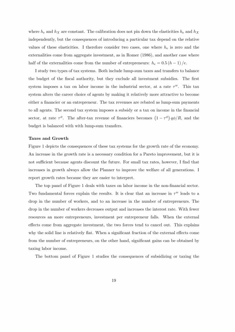
Taxes and Growth

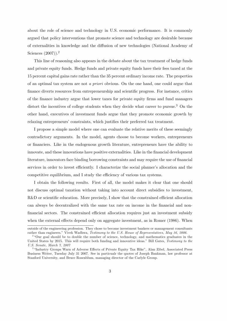
Figure 1 depicts the consequences of these tax systems for the growth rate of the economy.

An increase in the growth rate is a necessary condition for a Pareto improvement, but it is

not sufficient because agents discount the future. For small tax rates, however, I find that

increases in growth always allow the Planner to improve the welfare of all generations. I

report growth rates because they are easier to interpret.

The top panel of Figure 1 deals with taxes on labor income in the non-financial sector.

Two fundamental forces explain the results. It is clear that an increase in τw leads to a

drop in the number of workers, and to an increase in the number of entrepreneurs. The

drop in the number of workers decreases output and increases the interest rate. With fewer

resources an more entrepreneurs, investment per entrepreneur falls. When the external

effects come from aggregate investment, the two forces tend to cancel out. This explains

why the solid line is relatively flat. When a significant fraction of the external effects come

from the number of entrepreneurs, on the other hand, significant gains can be obtained by

taxing labor income.

The bottom panel of Figure 1 studies the consequences of subsidizing or taxing the

19

financial sector.12 When τφ decreases, more agents become financiers. This decreases the

number of workers and entrepreneurs, and increases the interest rate. While the number of

entrepreneurs falls, investment per entrepreneur increases because the financial constraints

are relaxed. The effect on aggregate investment is theoretically ambiguous, but in practice

aggregate investment increases. As a consequence, when he = 0, subsidizing the financial

sector increases the growth rate of the economy. When he = 0.5 (h− 1) /e, the fall in e andthe increase in X mostly cancel out. Of course, if we were to consider the extreme case

where hX = 0, it would be optimal to tax the financial sector. However, in this case, the

top panel suggests that it would be even more efficient to tax labor income in the industrial

sector.

The influence of the nature of the external effects on the optimal tax system sheds light

on the current debate regarding the taxation of private equity funds. During his Senate

Finance Committee hearing, Bruce Rosenblum, managing director of the Carlyle Group, a

Washington-based private equity fund, argued that, if the tax rate is increased, some deals

will not be done, “there will be entrepreneurs that won’t get funded and turnarounds that

won’t get undertaken.”13 On the other hand, Robert H. Frank argues that “No one denies

that the talented people who guide capital to its most highly valued uses perform a vital

service for society. But at any given moment, there are only so many deals to be struck.

Sending ever larger numbers of our most talented graduates out to prospect for them has a

high opportunity cost, yet adds little economic value. By making the after-tax rewards in the

investment industry a little less spectacular, the proposed legislation would raise the attrac-

tiveness of other career paths, ones in which extra talent would yield substantial gains.”14

In essence, one argues that aggregate investment is elastic and is the variable we should

care about, while the other argues that it is not very elastic and that the number of en-

trepreneurs is the variable of interest. The model makes is clear why they reach opposite

conclusions regarding the optimal taxation of the financial sector.

12The magnitudes in panels 1a and 1b are not comparable because the financial sector is much smallerthan the industrial sector, so that a tax rate τw of 1% involves transfers equivalent to a tax rate τφ of morethan 10%.13“Industry Groups Warn of Adverse Effects of Private Equity Tax Hike”, by Alan Zibel, Associated Press

Business Writer, Tuesday July 31 2007.14A Career in Hedge Funds and the Price of Overcrowding, The New York Times, July 5, 2007.

20

5 Conclusion

I have studied an economy with career choices, financial constraints and externalities from

innovation and entrepreneurship. The implementation of the second best requires invest-

ment subsidies to the extent that there are externalities linked to aggregate investment,

and subsidies to entrepreneurship or to scientific education to the extent that there are

externalities linked to the number of entrepreneurs and scientists. Once these subsidies are

in place, it is optimal to set exactly the same tax rate on labor income in the financial and

non-financial sectors, even in the presence of binding credit constraints.

When the second best subsidies are not feasible, the model sheds light on the two

economic forces that determine the efficiency of subsidizing the financial sector. On the

one hand, subsidizing the financial sector increases the investments that entrepreneurs can

undertake. On the other hand, it decreases the number of entrepreneurs by attracting more

individuals to the financial sector. In the quantitative analysis, I find that, starting from

a competitive economy without taxes, the introduction of a subsidy to the financial sector

increases the growth rate of the economy in the benchmark case where the external effects

depend on aggregate investment and R&D.

21

References

Aghion, P., and P. Howitt (1998): Endogenous Growth Theory. MIT Press, Cambridge,

Massachusetts.

Allen, F., and D. Gale (1994): Financial Innovation and Risk Sharing. MIT Press,

Cambridge, MA.

Arrow, K. J. (1962): “The Economic Implications of Learning by Doing,” Review of

Economic Studies, 29, 155—173.

Barro, R. J., and X. Sala-i-Martin (2004): Economic Growth. MIT Press, Cambridge,

Massachusetts.

Baumol, W. J. (1990): “Entrepreneurship: Productive, Unproductive, and Destructive,”

Journal of Political Economy, 98, 893—921.

Bencivenga, V. R., and B. D. Smith (1991): “Financial Intermediation and Endogenous

Growth,” Review of Economic Studies, 58, 195—209.

Boyd, J. H., and E. C. Prescott (1986): “Financial Intermediary Coalitions,” Journal

of Economic Theory, 38, 211—232.

Diamond, D. W. (1984): “Financial Intermediation and Delegated Monitoring,” Review

of Economic Studies, 51, 393—414.

Duffie, D., and R. Rahi (1995): “Financial Market Innovation and Security Design: An

Introduction,” Journal of Economic Theory, 65, 1—42.

Freixas, X., and J.-C. Rochet (1997): Microeconomics of Banking. MIT Press, Cam-

bridge.

Greenwood, J., and B. Jovanovic (1990): “Financial Development, Growth, and the

Distribution of Income,” Journal of Political Economy, 98, 1076—1107.

Greenwood, J., J. M. Sanchez, and C. Wang (2007): “Financing Development; The

Role of Information Costs,” Working Paper, University of Pennsylvania.

22

Griliches, Z. (1979): “Issues in Assessing the Contribution of Research and Development

to Productivity Growth,” Bell Journal of Economics, 10(1), 92—116.

Holmström, B., and J. Tirole (1997): “Financial Intermediation, Loanable Funds and

the Real Sector,” Quarterly Journal of Economics, 112, 663—691.

Khan, A. (2001): “Financial Development and Economic Growth,” Macroeconomic Dy-

namics, 5, 413—433.

King, R. G., and R. Levine (1993): “Finance and Growth: Schumpeter Might Be Right,”

Quarterly Journal of Economics, 108(3), 717—737.

Levine, R. (1991): “Stock Markets, Growth, and Tax Policy,” Journal of Finance, 46,

1445—1465.

(2005): “Finance and Growth: Theory and Evidence,” in Handbook of Economic

Growth, ed. by P. Aghion, and S. N. Durlauf, vol. 1A, pp. 865—934. Elsevier, Amsterdam.

Lucas, R. E. (1988): “On the Mechanics of Economic Development,” Journal of Monetary

Economics, 22, 3—42.

Moskowitz, T. J., and A. Vissing-Jorgensen (2002): “The Return to Entrepreneurial

Investment: A Private Equity Puzzle?,” American Economic Review, 92(4), 745—778.

Murphy, K. M., A. Shleifer, and R. W. Vishny (1991): “The Allocation of Talent:

Implications for Growth,” The Quarterly Journal of Economics, 106, 503—530.

National Academy of Sciences (2007): Rising Above the Gathering Storm. Committee

on Science, Engineering, and Public Policy.

Philippon, T. (2007): “The Equilibrium Size of the Financial Sector,” NBER Working

Paper No. 13405.

Philippon, T., and A. Resheff (2007): “Skill Biased Financial Development: Educa-

tion, Wages and Occupations in the U.S. Financial Sector,” Working Paper, New York

University.

23

Philippon, T., and Y. Sannikov (2007): “Financial Development, IPOs, and Business

Risk,” mimeo, NYU.

Plumley, A. (2004): “Overview of the Federal Tax Gap,” Discussion paper, US Depart-

ment of the Treasury, Internal Revenue Service, Washington, DC.

Romer, P. M. (1986): “Increasing Returns and Long Run Growth,” Journal of Political

Economy, 94, 1002—1037.

Sheshinski, E. (1967): “Optimal Accumulation with Learning by Doing,” in Essays on

the Theory of Optimal Growth, ed. by K. Shell, Cambride, Mass. MIT Press.

Tufano, P. (2004): “Financial Innovation,” in The Handbook of the Economics of Finance,

ed. by M. H. George Constantinides, and R. Stulz. North Holland.

Weisbach, D. A. (2007): “The Taxation of Carried Interests In Private Equity Partner-

ships,” The University of Chicago Law School.

24

A Proof of Lemma 1

Fix the number of entrepreneurs et and aggregate investment Xt. From the law of motion(6), this implies that at+1 is given. Let i = 0 denote a particular entrepreneur. Considerthe following program, denoted SP0:

maxu¡c01t¢+ βu

¡c02t+1

¢subject to the set of constraints Z

i∈eci1t ≤ Ct : {λt}Z

i∈eci2t+1 − f

µat+1nt+1,

Zi∈et

g¡at, x

it

¢di

¶≤ −Ct+1 : {λt+1}Z

i∈etmi

t ≤ Mt : {θt}Zi∈et

xitdi ≤ Xt : {χt}

zxit − atq¡mi

t

¢− ci2,t+1 ≤ 0 :©μitª

Ut − u¡ci1,t¢+ βu

¡ci2,t+1

¢ ≤ 0 :©γitª

And, to be consistent with the constraint that all agents must receive the same utility inthe original problem, Ut is chosen such that

Ut = u¡c01t¢+ βu

¡c02t+1

¢For given values of et, bt and Xt, the first two constraints keep the allocation of consumptionto the other agents feasible. The other constraint are satisfied by the original program ofthe social planner. For the solution of the planner to be optimal, the allocation amongentrepreneur must therefore solve (SP0). The optimality conditions are:

u0¡ci1,t¢

βu0³ci2,t+1

´ =λt

λt+1 − μit

λt+1∂g¡at, x

it

¢∂xit

∂ft+1∂kt+1

= μitz + χt

θt = μitatq0 ¡mi

t

¢Let us show that μit must be the same for all i ∈ et. Consider two entrepreneurs

i and j and suppose that the enforcement constraint binds more for i and than for j:μit > μjt . Therefore u

0 ¡ci1t¢ /u0 ³cj1t´ > u0¡ci2t+1

¢/u0³cj2t+1

´. Since both i and j receive

the same ex-ante utility, we must have ci1t < cj1t and ci2t+1 > cj2t+1. Since μit > μjt andq (.) is concave, it must be the case that mi

t ≥ mjt . Therefore zx

it = atq

¡mi

t

¢+ ci2,t+1 >

atq³mj

t

´+ cj2,t+1 ≥ zxjt and xit > xjt . The optimality condition for investment implies that

∂g¡at, x

it

¢/∂xit > ∂g

³at, x

jt

´/∂xjt . Since g is concave, this implies that xit < xjt , which

contradicts the previous inequality. Therefore, μit must be the same for all i ∈ et. QED.

25

B Proof of Proposition 1

For bankers and workers, the consumption/saving decision is unchanged and the careerchoice condition becomes:

(1− τwt )Rtat∂ft∂nt

=³1− τφt

´ϕt+1.

The program of the entrepreneur changes because her budget constraint becomes:

ce1t +ce2t+1Rt

+ (1− τxt )xt + (1− τ et ) atse ≤ g (at, xt)

Rt

∂ft+1∂kt+1

− ϕt+1mt

Rt.

The Euler equation of the entrepreneur does not change, but the first order condition forinvestment becomes:

φtz + (1− τxt )Rt =∂gt∂xt

∂ft+1∂kt+1

. (28)

The optimal choice of monitoring is still:

atφtq0 (mt) = ϕt+1.

We are looking for tax rates¡τφ, τw, τx

¢that decentralize the SP outcome. Because the

Euler equations of workers and bankers have not changed, we must have the same R.Similarly, from the Euler equation of the entrepreneurs, we must have the same φ. Fromthe career choice of workers and financiers, it follows that:

τφt = τwt .

The tax rate on labor income is the same inside or outside the financial services industry.From (20), we see that Rt + φtz =

∂gt∂xt

∂ft+1∂kt+1

+ πt+1∂ht∂Xt. From (28), we see that Rt + φtz =

∂gt∂xt

∂ft+1∂kt+1

+ τxtRt. Therefore, we must have:

τxt =πt+1Rt

∂ht∂Xt

.

Finally, to get the correct number of entrepreneurs, we must ensure that the career choicecoincides with the choice of the social planner. With taxes, the career choice is:

xt+atse+ce1t−c1t+at

∂ft∂nt

+ce2t+1 − c2t+1

Rt=

gtRt

∂ft+1∂kt+1

−atφtbtetRt

q0t+atµτxt

xtat+ τ ets

e + τw∂ft∂nt

¶.

Comparing with (21), we see that the two equations are equivalent if and only if:

τxtxtat+ τ ets

e + τw∂ft∂nt

=πt+1Rt

µ∂ht∂et

+xtat

∂ht∂Xt

¶.

Using the optimal value of τxt , this leads to:

τ etse + τwt

∂ft∂nt

=πt+1Rt

∂ht∂et

.

I have shown the necessary conditions for implementation. It is easy to check that they aresufficient as well, since all the other equilibrium conditions are also satisfied. QED.

26

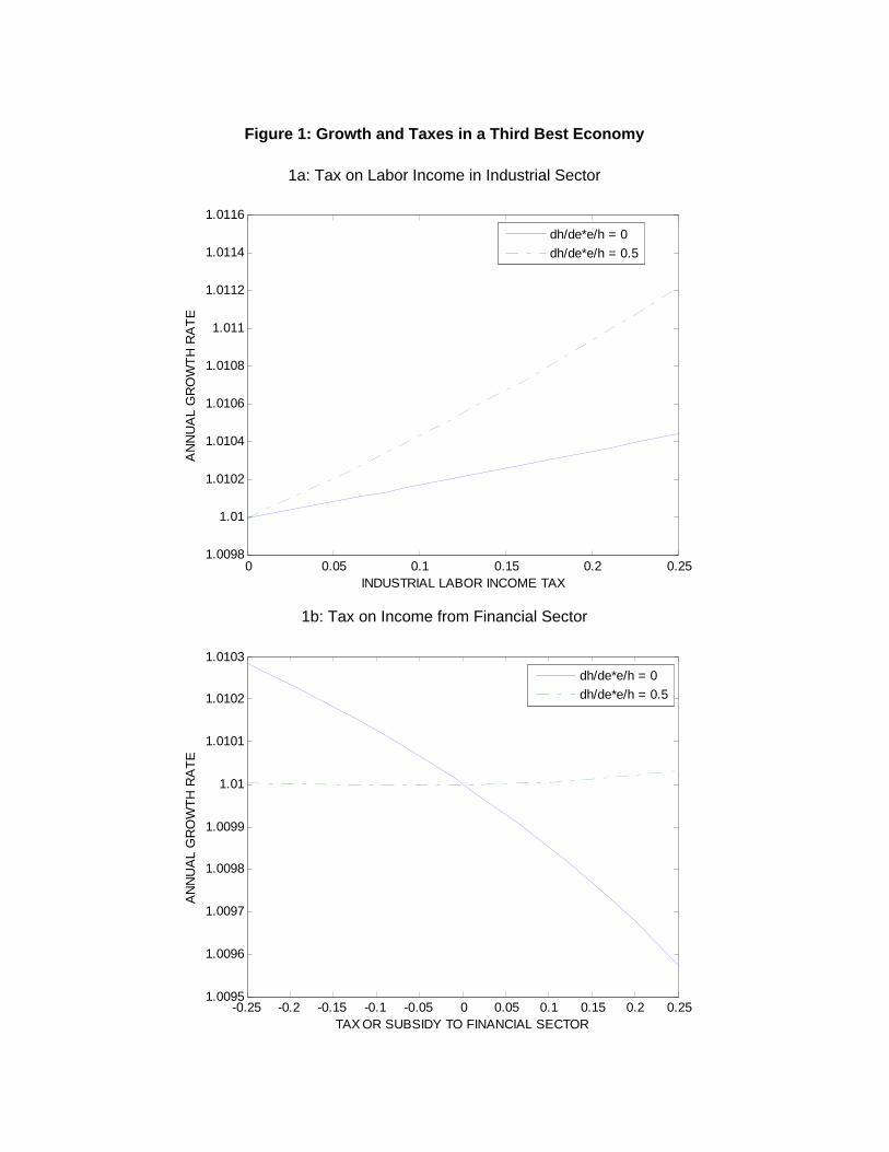
Figure 1: Growth and Taxes in a Third Best Economy

1a: Tax on Labor Income in Industrial Sector

1b: Tax on Income from Financial Sector

0 0.05 0.1 0.15 0.2 0.251.0098

1.01

1.0102

1.0104

1.0106

1.0108

1.011

1.0112

1.0114

1.0116

INDUSTRIAL LABOR INCOME TAX

AN

NU

AL

GR

OW

TH R

ATE

dh/de*e/h = 0dh/de*e/h = 0.5

-0.25 -0.2 -0.15 -0.1 -0.05 0 0.05 0.1 0.15 0.2 0.251.0095

1.0096

1.0097

1.0098

1.0099

1.01

1.0101

1.0102

1.0103

TAX OR SUBSIDY TO FINANCIAL SECTOR

AN

NU

AL

GR

OW

TH R

ATE

dh/de*e/h = 0dh/de*e/h = 0.5