Embed Size (px)
Citation preview
Financials in Football: Evaluations, Bonds and Derivatives
Gabriele Saponaro
Matricola: 216411
Matriculation Year: 2017
Academic Year: 2019/2020
Supervised by Professor Andrea Pozzi
(Applied Statistics & Econometrics)

Financials in Football: Evaluations, Bonds and Derivatives - Gabriele Saponaro 216411
2
I would like to begin this thesis by thanking Deloitte&Tousche for the
opportunities that provides, with summer internships, to many young
and inexperienced undergraduates, which have the opportunity to
discover the working environment and to develop skills that will be
fundamental in future experiences. Thanks to that experience I was
able to analyze in depth topics of my area of interest and also
understand the logic of the consultant sector, in which would be
fascinating to work in the near future. Especially due to the team-
building activities and stimulating atmosphere, favored by the Head of
Financial Evaluation Department, Mr. Marco Vulpiani, I was able to
establish sincere relationships with some of Deloitte’s employees, that
supported me in my experience. I would like also to thank
Deloitte&Tousche for allowing to include the work brought on for
“Money League” project in Chapter 1 of this Thesis.
I would like to thank also AS Roma S.P.A, that gave me the opportunity
to present my work in a dedicated meeting with the Chief Executive
Office Mr Guido Fienga and the Chef Financial Officer Mr Giorgio
Francia. I hope that my work has contributed to stimulate additional
investigation in a sector in continuous financial development.
Financials in Football: Evaluations, Bonds and Derivatives - Gabriele Saponaro 216411
3
Financials in Football: Evaluations, Bonds and Derivatives
INDEX
INTRODUCTION / EXECUTIVE SUMMARY .......................................................................... 4
CHAPTER 1 - DELOITTE MONEY FOOTBALL LEAGUE TODAY .............................................. 12
GENERAL OVERVIW ........................................................................................................................... 12
FUTURE PREDICTIONS ....................................................................................................................... 17
CHAPTER 2 - EVALUATION METHODS OF SOCCER CLUBS ................................................. 20
METHODOLOGICAL APPROACHES .............................................................................................................. 20
KPMG APPROACH ................................................................................................................................. 20
FORBES APPROACH .............................................................................................................................. 23
MULTIPLES EV / REVENUES ..................................................................................................................... 24
COMPARISON KPMG VS FORBES ............................................................................................................ 27
CHAPETR 3 - FINANCIAL ECONOMICS OF FOOTBALL TEAMS ............................................ 29
INDEXES OF FOOTBALL TEAMS .................................................................................................................. 29
FINANCIAL STATEMENTS AS INFORMATION AND MEASURE INSTRUMENT.......................................................... 31
CASE STUDY: REAL MADRID, STILL THE TEAM TO BEAT? ................................................................................ 32
CHAPTER 4 - IAS 39 AND IFRS 9 ....................................................................................... 37
SCOPE OF APPLICATION OF IAS 39...................................................................................................... 37
RECOGNITION AND MEASUREMENT OF FINANCIAL INSTRUMENTS ................................................................... 41
EVALUATION ...................................................................................................................................... 44
COVERAGE OPERATIONS ................................................................................................................... 52
IFRS 9 ................................................................................................................................................. 55
CHAPETR 5 – INNOVATIVE LIABILITIES & MARK TO MARKET VALUES ............................... 56
KICK-BONDS INDEXED TO PERFORMANCE ................................................................................................... 56
MERTON MODEL & SECURITY MARKET LINE APPLICATIONS ........................................................................... 57
MARKET VALUE TROUGH BLACK & SCHOLES DERIVATIVES EVALUATION .......................................................... 60
CHAPTER 6 - BLACK & SCHOLES EQUATION ..................................................................... 62
PROBABILITY SPACES, FILTRATIONS, PROCESSES AND CONDITIONAL EXPECTATION .............................................. 62
BROWNIAN MOTION AND ITO’S LEMMA .................................................................................................... 72
THE BLACK-SCHOLES’ WORLD .................................................................................................................. 79
VALUATION OF OPTIONS IN BLACK-SCHOLES ............................................................................................... 88
CHAPTER 7 – NEW FINANCIAL FRONTIER: A.S. ROMA CASE STUDY .................................. 97
CONCLUSION ................................................................................................................ 104
BIBLIOGRAPHY ............................................................................................................. 105
Financials in Football: Evaluations, Bonds and Derivatives - Gabriele Saponaro 216411
4
Introduction / Executive Summary
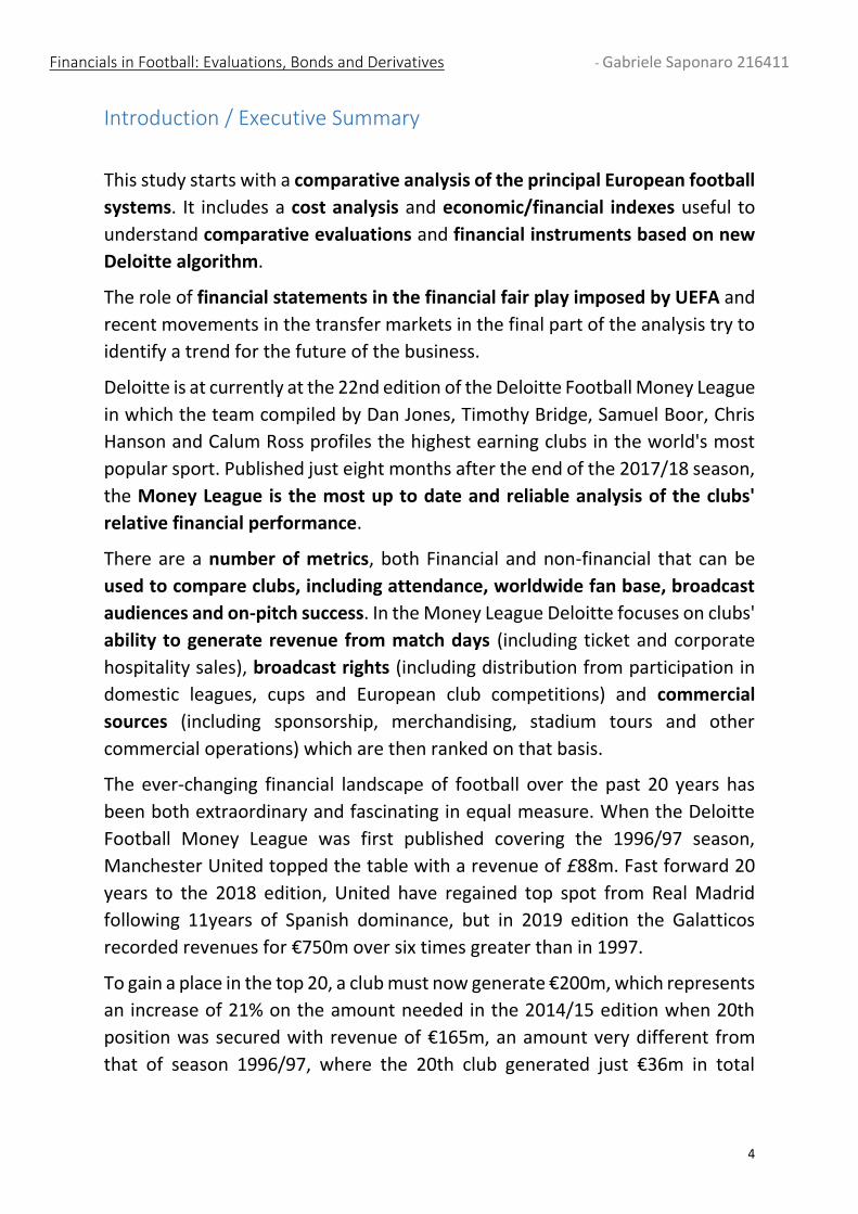
This study starts with a comparative analysis of the principal European football
systems. It includes a cost analysis and economic/financial indexes useful to
understand comparative evaluations and financial instruments based on new
Deloitte algorithm.
The role of financial statements in the financial fair play imposed by UEFA and
recent movements in the transfer markets in the final part of the analysis try to
identify a trend for the future of the business.
Deloitte is at currently at the 22nd edition of the Deloitte Football Money League
in which the team compiled by Dan Jones, Timothy Bridge, Samuel Boor, Chris
Hanson and Calum Ross profiles the highest earning clubs in the world's most
popular sport. Published just eight months after the end of the 2017/18 season,
the Money League is the most up to date and reliable analysis of the clubs'
relative financial performance.
There are a number of metrics, both Financial and non-financial that can be
used to compare clubs, including attendance, worldwide fan base, broadcast
audiences and on-pitch success. In the Money League Deloitte focuses on clubs'
ability to generate revenue from match days (including ticket and corporate
hospitality sales), broadcast rights (including distribution from participation in
domestic leagues, cups and European club competitions) and commercial
sources (including sponsorship, merchandising, stadium tours and other
commercial operations) which are then ranked on that basis.
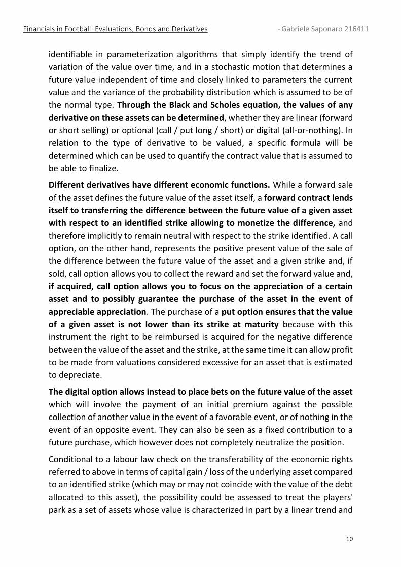
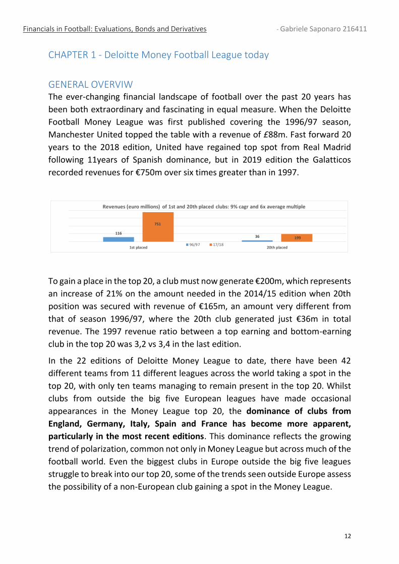
The ever-changing financial landscape of football over the past 20 years has
been both extraordinary and fascinating in equal measure. When the Deloitte
Football Money League was first published covering the 1996/97 season,
Manchester United topped the table with a revenue of £88m. Fast forward 20
years to the 2018 edition, United have regained top spot from Real Madrid
following 11years of Spanish dominance, but in 2019 edition the Galatticos
recorded revenues for €750m over six times greater than in 1997.
To gain a place in the top 20, a club must now generate €200m, which represents
an increase of 21% on the amount needed in the 2014/15 edition when 20th
position was secured with revenue of €165m, an amount very different from
that of season 1996/97, where the 20th club generated just €36m in total
Financials in Football: Evaluations, Bonds and Derivatives - Gabriele Saponaro 216411
5
revenue. The 1997 revenue ratio between a top earning and bottom-earning
club in the top 20 was 3,2 vs 3,4 in the last edition.
In the 22 editions of Deloitte Money League to date, there have been 42
different teams from 11 different leagues across the world taking a spot in the
top 20, with only ten teams managing to remain present in the top 20. Whilst
clubs from outside the big five European leagues have made occasional
appearances in the Money League top 20, the dominance of clubs from
England, Germany, Italy, Spain and France has become more apparent,
particularly in the most recent editions. This dominance reflects the growing
trend of polarization, common not only in Money League but across much of the
football world. Even the biggest clubs in Europe outside the big five leagues
struggle to break into our top 20, some of the trends seen outside Europe assess
the possibility of a non-European club gaining a spot in the Money League.
CHAPTER 1 concludes by showing how the comparison in the next few years will
develop precisely on the financial equilibrium introduced through the new
regulation of the Financial Fair Play of UEFA which will develop clubs’ business
and financial equilibrium and the acknowledgement in the financial statements.
The introduction of financial fair play beyond the evident sporting value aimed
at guaranteeing a more level playing field by aiming to avoids leagues dominated
by magnates with inexhaustible capital has a financial interest in guaranteeing
interest around the football system that remains dependent of the
competitiveness of clubs in different leagues. As has been highlighted in the
analysis of the major leagues, in fact, it’s precisely where there is competition
that the customer is interested in spending money to follow a sporting event at
the stadium or on television. For example a better redistribution of the
television rights among the different clubs increases competition and interest of
the fans that will then increase the “broadcast cake” to be served in the
following years.
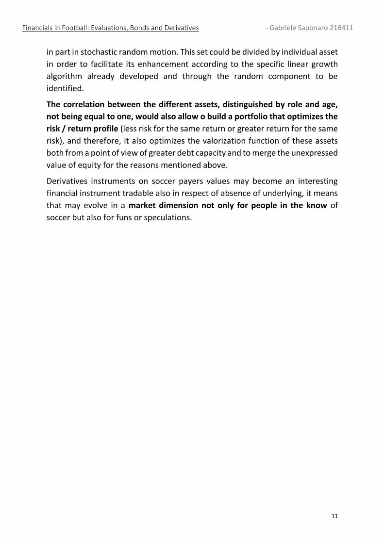
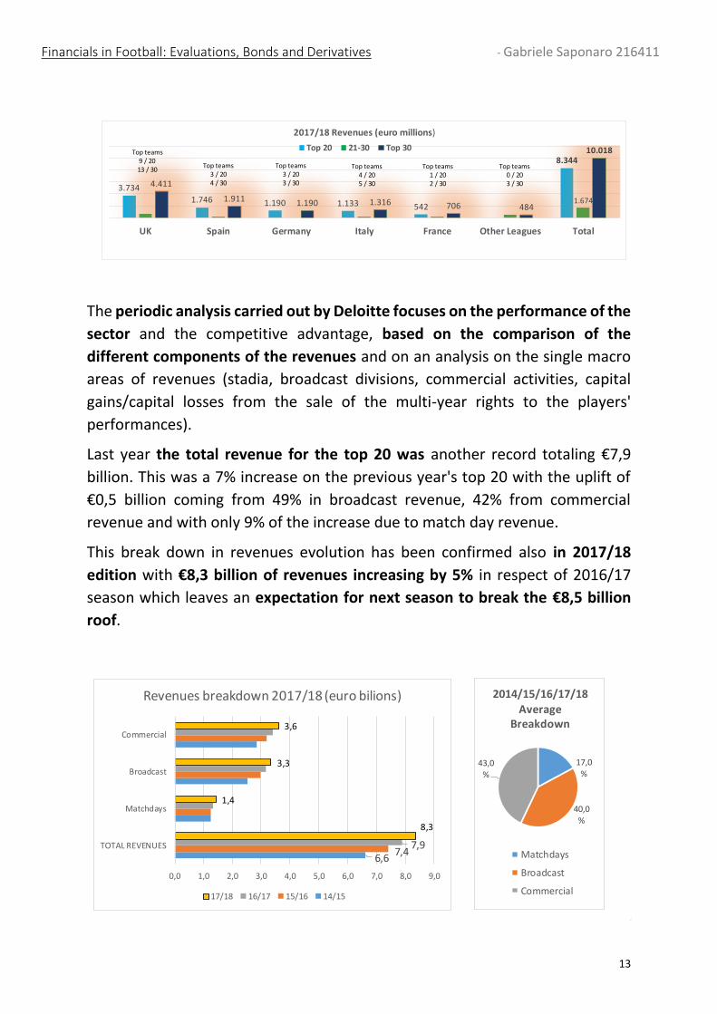
The periodic analysis carried out by Deloitte focuses on the performance of the
sector and the competitive advantage, based on the comparison of the
different components of the revenues and on an analysis on the single macro
areas of revenues (stadia, broadcast divisions, commercial activities, capital
gains/capital losses from the sale of the multi-year rights to the players'
performances).
Financials in Football: Evaluations, Bonds and Derivatives - Gabriele Saponaro 216411
6
Soccer clubs are valued based upon numerous factors not limited to the main
multiple of Enterprise Value (equity plus debt) on revenues (CHAPTER 2).
Income is generated from broadcast agreements, premium seating and match
day ticket sales, media, brand and product licensing, and merchandise and
concessions sales. Crucial is the identification of the value of the team players
that depends on performance, role, age as well as behaviour. As seen in the
accounting analysis there are different way to represent that in the balance
sheet, but what is difficult is to predict the value of the players for the future
because of the numerous variables involved in the analysis.
Starting from the analysis obtained from the documentation produced by
Deloitte summarized on a three-year basis and also trying to identify a
prospective trend, (in CHAPTER 3) a comparison is made between economic
and financial evidence on aggregated economic data of the leagues and
analyzing the items that characterize the budget of a football firm also
including a series of industry efficiency indicators.
Also in relation to the entry into force of the financial fair play, in order to
understand what are the appropriate methods of evaluation for football clubs
(and in particular for the player park), an investigation has been carried out on
possible financial instruments that according International Accounting
Standards IAS 39 (CHAPETR 4) could be able to book in the balance sheet the
mark to market of the value of the team players.
It helps also in debt raising capacity because when the club performance is
constantly at high levels the financial capacity will accordingly increase in the
long run. But if the performance is not satisfying may be difficult to earn stable
revenues to devote to the debt service and for this reason the capital markets
look with diffidence at financing football club on unsecured basis.
A possible solution has been discovered by Kick-bonds that link in a positive
relation the remuneration of the bond with the performance of the team
(CHAPTER 5). In this way the clubs can attract financial interest from the market
and can benefit of a sort of natural hedge because it commits themselves to pay
more only if the performance is good.
The platform Kickoffers, created in partnership with Deloitte, has structured an
algorithm in order to quantify the performance of the team and of the football
player linked to remuneration of these kick-bonds. If the player’s disposal would
generate a gain in respect of initial evaluation coming from the Deloitte
Financials in Football: Evaluations, Bonds and Derivatives - Gabriele Saponaro 216411
7
algorithm, an extra bonus will be paid to the investors. The first experience of
Deloitte algorithm application has been the one of Italian soccer club Chievo
which listed its financial bonds and not its shares as Juventus, Lazio and Roma.
In my 2018 experience in Deloitte when I analyzed the financial assessments of
the football teams on multiples, I understood as predictable may be the
component of linear growth of a player's value, but also that a random
component is part of soccer players evaluation (for example used as a reward
on the coupon of a bond issue parameterized to the surplus value on a specific
player).
On the other hand in 2019, both in my “Analysis and Management of Financial
Risk” course at the London School of Economics and in my “Financial
Mathematics” studies at the Mathematics Department of Edinburgh, I studied
how, under certain conditions that seem to be able to apply also on the
performance of the players' value, you can price the value of a derivative
contract which has as its underlying the price of an asset that moves over time
according to an identified trend but also in relation to its average value and
volatility.
The Black & Scholes model, that I analyzed with the help of Professor Biagini and
her notes (CHAPTER 6), is applied continuously and involves the use of statistical
tools and probability distribution that I have had the opportunity to deepen in
my studies. I therefore thought I could extend the contents of my thesis also to
an analysis of the now widespread tools of options on players (both in terms of
the right to buy and to sell) with high statistical-mathematical value.
From an economic-financial modelling point of view, the Merton model
identifies the market value of a company (Equity Value, or Market
Capitalization if listed) as a call option on the value of the assets (entire
corporate value or Enterprise Value) with strike price equal to the value of the
debt and with expiry the debt maturity. The present value of the Equity is
expressed as the present value of the average probable difference between the
value of the entire asset at the maturity of the debt and the value of the debt
itself. Equity can have a positive present value even if the current value of the
assets is lower than the current value of the debt because, at the maturity of the
debt, the market value of the assets (Enterprise Value) can exceed, with a certain
probability, the debt value that grows only with the interest rate.
Financials in Football: Evaluations, Bonds and Derivatives - Gabriele Saponaro 216411
8
The basic assumption of the methodology is that, if the asset company value
should be lower than the debt value, the property would have no economic
interest in continuing in the company activity and therefore the value would be
at the minimum zero given it is not obliged to proceed with capital increases,
unless there is a prospective value to be protected. If this difference were
instead positive, the expected value of the payoff of this difference discounted
according to a risk-neutral approach would be the value of the Equity itself.
Basically, from this approach, it emerges just how the current value of the
company can be higher than the current difference between assets and
liabilities since, with a certain probability, the assets will grow more than the
debt capitalized for its contractual interest rate.
It is an approach based on market evidence that leads to an evaluation of an
equivalent company to that of discounting the company's future cash flows by
means of a discount factor that takes into account of the uncertainty of these
flows according to an adequate relationship between risk (variance of cash
flows) and return (discount rate) which must be on the Security Market Line. If
this value were contractually divisible into sub-sets of assets, the diversification
effect that allows to optimize the risk / return profile by determining the
optimal portfolios (which represent the efficient Markowitz frontier) must also
be considered.
If the valuation of the Equity can be conceptualized as a call option on the
underlying corporate value compared to a strike represented by the value of the
debt at maturity, by extension the value of the Equity can be divided into
subsets represented specific categories of assets with which to associate
specific values: i) the most certain part using, instead, for the enhancement the
approach of cash flows discounted at an interest rate that reflects the modest
variance of these flows; ii) the most random (but also most market and therefore
verifiable) part following the approach of the call options to evaluate their value.
Certainly the part with the most certain cash flows lends itself better than the
random one to be able to sustain the debt in terms of repayable prospect but, if
debt or mezzanine funds are identified in the market with appetite for
individually transferable assets and with a market value that can be
parameterized, the advantages in using this valuation method would be
different. From the point of view of the company's debt capacity, access to the
specialized, alternative or additional debt market to the banking and bond
market could be obtained. Investors interested in the finance ability of even a
Financials in Football: Evaluations, Bonds and Derivatives - Gabriele Saponaro 216411
9
single asset with a formula similar to that of the pledge (if not of the financial
leasing) could be found in which the repayment is collateralized by the value of
the asset at maturity of the debt and whose remuneration could be indexed the
payoff at maturity equal to the difference between the value of the asset and
the capitalized debt (kick bond).
From an Equity value point of view, the future value of the more random assets
could emerge immediately, despite the International Accounting Standards do
not allow to be valued before their realization according to the logic of
prudence (IAS 39), unless this derives from a market exchange contract of this
value.
For example, you could enter into forward contracts that fix the price of the
asset at maturity (without predicting its sale) or even assign call options on
certain assets that would collect premiums and reveal the unexpressed values
of these assets as: i) the cash flow method cannot capture the specificity of these
assets, necessarily having to reason for average values; ii) the international
accounting standards do not allow their valuation in the financial statements
until realization / marketing.
If soccer companies do not want to set forward prices or transfer the rights on
the value of the assets with respect to a certain strike (which may even be higher
than the value of the specific debt that you can allocate on these assets), they
could also consider issuing shares privileged with special rules that factor the
rights regarding the future sale of certain assets with respect to a specific strike
assigned to them. In this last way, differently from the previous ones, the value
linked to the optionality of these assets could not be reported in the financial
statements (which would instead be very functional for the issue of new debt),
but the value not expressed in specific terms could still be valorized of greater
equity, the enhancement of which occurs through free trade between the
parties.
The market equity value is already, per se, an expression of the presence of an
asset value not reflected in the financial statements due to prudential
constraints imposed by the IAS, however a more specific identification of this
subset would have a positive effect on the capitalization suffering from
penalizing weightings and discount for uncertainty.
The assets to be valued according to the optional approach are those with
greater uncertainty and for which a linear motion can be distinguished,
Financials in Football: Evaluations, Bonds and Derivatives - Gabriele Saponaro 216411
10
identifiable in parameterization algorithms that simply identify the trend of
variation of the value over time, and in a stochastic motion that determines a
future value independent of time and closely linked to parameters the current
value and the variance of the probability distribution which is assumed to be of
the normal type. Through the Black and Scholes equation, the values of any
derivative on these assets can be determined, whether they are linear (forward
or short selling) or optional (call / put long / short) or digital (all-or-nothing). In
relation to the type of derivative to be valued, a specific formula will be
determined which can be used to quantify the contract value that is assumed to
be able to finalize.
Different derivatives have different economic functions. While a forward sale
of the asset defines the future value of the asset itself, a forward contract lends
itself to transferring the difference between the future value of a given asset
with respect to an identified strike allowing to monetize the difference, and
therefore implicitly to remain neutral with respect to the strike identified. A call
option, on the other hand, represents the positive present value of the sale of
the difference between the future value of the asset and a given strike and, if
sold, call option allows you to collect the reward and set the forward value and,
if acquired, call option allows you to focus on the appreciation of a certain
asset and to possibly guarantee the purchase of the asset in the event of
appreciable appreciation. The purchase of a put option ensures that the value
of a given asset is not lower than its strike at maturity because with this
instrument the right to be reimbursed is acquired for the negative difference
between the value of the asset and the strike, at the same time it can allow profit
to be made from valuations considered excessive for an asset that is estimated
to depreciate.
The digital option allows instead to place bets on the future value of the asset
which will involve the payment of an initial premium against the possible
collection of another value in the event of a favorable event, or of nothing in the
event of an opposite event. They can also be seen as a fixed contribution to a
future purchase, which however does not completely neutralize the position.
Conditional to a labour law check on the transferability of the economic rights
referred to above in terms of capital gain / loss of the underlying asset compared
to an identified strike (which may or may not coincide with the value of the debt
allocated to this asset), the possibility could be assessed to treat the players'
park as a set of assets whose value is characterized in part by a linear trend and
Financials in Football: Evaluations, Bonds and Derivatives - Gabriele Saponaro 216411
11
in part in stochastic random motion. This set could be divided by individual asset
in order to facilitate its enhancement according to the specific linear growth
algorithm already developed and through the random component to be
identified.
The correlation between the different assets, distinguished by role and age,
not being equal to one, would also allow o build a portfolio that optimizes the
risk / return profile (less risk for the same return or greater return for the same
risk), and therefore, it also optimizes the valorization function of these assets
both from a point of view of greater debt capacity and to merge the unexpressed
value of equity for the reasons mentioned above.
Derivatives instruments on soccer payers values may become an interesting
financial instrument tradable also in respect of absence of underlying, it means
that may evolve in a market dimension not only for people in the know of
soccer but also for funs or speculations.
Financials in Football: Evaluations, Bonds and Derivatives - Gabriele Saponaro 216411
12
CHAPTER 1 - Deloitte Money Football League today
GENERAL OVERVIW The ever-changing financial landscape of football over the past 20 years has
been both extraordinary and fascinating in equal measure. When the Deloitte
Football Money League was first published covering the 1996/97 season,
Manchester United topped the table with a revenue of £88m. Fast forward 20
years to the 2018 edition, United have regained top spot from Real Madrid
following 11years of Spanish dominance, but in 2019 edition the Galatticos
recorded revenues for €750m over six times greater than in 1997.
To gain a place in the top 20, a club must now generate €200m, which represents
an increase of 21% on the amount needed in the 2014/15 edition when 20th
position was secured with revenue of €165m, an amount very different from
that of season 1996/97, where the 20th club generated just €36m in total
revenue. The 1997 revenue ratio between a top earning and bottom-earning
club in the top 20 was 3,2 vs 3,4 in the last edition.
In the 22 editions of Deloitte Money League to date, there have been 42
different teams from 11 different leagues across the world taking a spot in the
top 20, with only ten teams managing to remain present in the top 20. Whilst
clubs from outside the big five European leagues have made occasional
appearances in the Money League top 20, the dominance of clubs from
England, Germany, Italy, Spain and France has become more apparent,
particularly in the most recent editions. This dominance reflects the growing
trend of polarization, common not only in Money League but across much of the
football world. Even the biggest clubs in Europe outside the big five leagues
struggle to break into our top 20, some of the trends seen outside Europe assess
the possibility of a non-European club gaining a spot in the Money League.
11636
751
199
1st placed 20th placed
Revenues (euro millions) of 1st and 20th placed clubs: 9% cagr and 6x average multiple
96/97 17/18
Financials in Football: Evaluations, Bonds and Derivatives - Gabriele Saponaro 216411
13
The periodic analysis carried out by Deloitte focuses on the performance of the
sector and the competitive advantage, based on the comparison of the
different components of the revenues and on an analysis on the single macro
areas of revenues (stadia, broadcast divisions, commercial activities, capital
gains/capital losses from the sale of the multi-year rights to the players'
performances).
Last year the total revenue for the top 20 was another record totaling €7,9
billion. This was a 7% increase on the previous year's top 20 with the uplift of
€0,5 billion coming from 49% in broadcast revenue, 42% from commercial
revenue and with only 9% of the increase due to match day revenue.
This break down in revenues evolution has been confirmed also in 2017/18
edition with €8,3 billion of revenues increasing by 5% in respect of 2016/17
season which leaves an expectation for next season to break the €8,5 billion
roof.
3.734
1.746 1.190 1.133 542
8.344
1.674
4.411
1.911 1.190 1.316 706 484
10.018
UK Spain Germany Italy France Other Leagues Total
2017/18 Revenues (euro millions)
Top 20 21-30 Top 30
Top teams3 / 204 / 30
Top teams3 / 203 / 30
Top teams4 / 205 / 30
Top teams1 / 202 / 30
Top teams0 / 203 / 30
Top teams9 / 2013 / 30
cagr 12-17
8,9%
6,67,4
7,9
8,3
1,4
3,3
3,6
0,0 1,0 2,0 3,0 4,0 5,0 6,0 7,0 8,0 9,0
TOTAL REVENUES
Matchdays
Broadcast
Commercial
Revenues breakdown 2017/18 (euro bilions)
17/18 16/17 15/16 14/15
17,0%
40,0%
43,0
%
2014/15/16/17/18 Average
Breakdown
Matchdays
Broadcast
Commercial
Financials in Football: Evaluations, Bonds and Derivatives - Gabriele Saponaro 216411
14
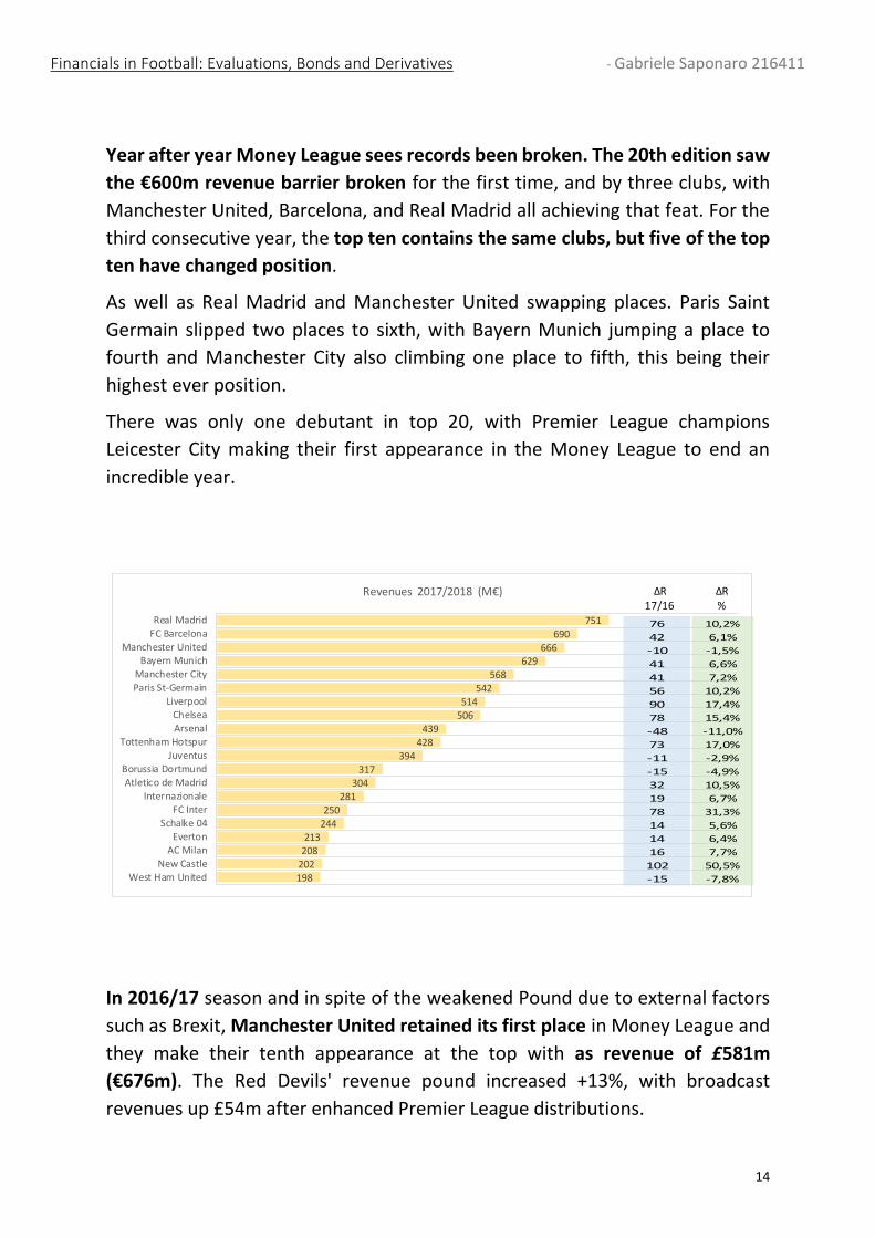
Year after year Money League sees records been broken. The 20th edition saw
the €600m revenue barrier broken for the first time, and by three clubs, with
Manchester United, Barcelona, and Real Madrid all achieving that feat. For the
third consecutive year, the top ten contains the same clubs, but five of the top
ten have changed position.
As well as Real Madrid and Manchester United swapping places. Paris Saint
Germain slipped two places to sixth, with Bayern Munich jumping a place to
fourth and Manchester City also climbing one place to fifth, this being their
highest ever position.
There was only one debutant in top 20, with Premier League champions
Leicester City making their first appearance in the Money League to end an
incredible year.
In 2016/17 season and in spite of the weakened Pound due to external factors
such as Brexit, Manchester United retained its first place in Money League and
they make their tenth appearance at the top with as revenue of £581m
(€676m). The Red Devils' revenue pound increased +13%, with broadcast
revenues up £54m after enhanced Premier League distributions.
751690
666629
568542
514506
439428
394317
304281
250244
213208
202198
Real MadridFC Barcelona
Manchester UnitedBayern Munich
Manchester CityParis St-Germain
LiverpoolChelseaArsenal
Tottenham HotspurJuventus
Borussia DortmundAtletico de Madrid
InternazionaleFC Inter
Schalke 04Everton
AC MilanNew Castle
West Ham United
Revenues 2017/2018 (M€)
76
42
-10
41
41
56
90
78
-48
73
-11
-15
32
19
78
14
14
16
102
-15
10,2%
6,1%
-1,5%
6,6%
7,2%
10,2%
17,4%
15,4%
-11,0%
17,0%
-2,9%
-4,9%
10,5%
6,7%
31,3%
5,6%
6,4%
7,7%
50,5%
-7,8%
ΔR17/16
ΔR%

Financials in Football: Evaluations, Bonds and Derivatives - Gabriele Saponaro 216411
15
Their crown was critical only because of pound depreciation (in 2016 equal to -
15%) with result that the gap between them and Real Madrid (with revenues
increase of + 8%) was just €1,7m, and the importance of the €3m additional
amount received from winning the Europa League Final is clearly evident.
Commercial revenue growth was limited in 2016/17, but Manchester United
with this revenue stream remained the club's largest and is over 30% more than
closest domestic rivals, Manchester City.
Manchester United's strong commercial growth coupled with a return to UEFA
Champions League saw them take the Money League crown keeping 5% far the
Barcelona who lost in the Money League ‘El Clasico’ by piping Real Madrid to
second position, by the smallest of margins.
2° best Band
1
2
3
4
5
6
7
8
9
10
11
12
13
14
15
16
17
18
19
20
21
22
23
24
25
26
27
28
29
30
14/15 15/16 16/17 17/18
RankingReal Madrid
FC Barcelona
Manchester United
Bayern Munich
Manchester City
Paris St-Germain
Liverpool
Chelsea
Arsenal
Tottenham Hotspur
Juventus
Borussia Dortmund
Atletico de Madrid
Internazionale
FC Inter
Schalke 04
Everton
AC Milan
New Castle
West Ham United
Top 3 Bands
Challengers' Band
Outsiders' Band
Financials in Football: Evaluations, Bonds and Derivatives - Gabriele Saponaro 216411
16
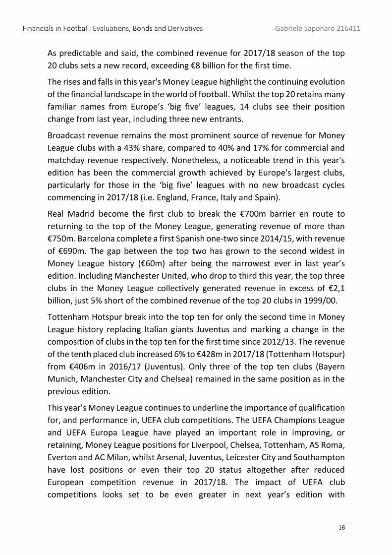
As predictable and said, the combined revenue for 2017/18 season of the top
20 clubs sets a new record, exceeding €8 billion for the first time.
The rises and falls in this year's Money League highlight the continuing evolution
of the financial landscape in the world of football. Whilst the top 20 retains many
familiar names from Europe’s ‘big five’ leagues, 14 clubs see their position
change from last year, including three new entrants.
Broadcast revenue remains the most prominent source of revenue for Money
League clubs with a 43% share, compared to 40% and 17% for commercial and
matchday revenue respectively. Nonetheless, a noticeable trend in this year's
edition has been the commercial growth achieved by Europe's largest clubs,
particularly for those in the ‘big five’ leagues with no new broadcast cycles
commencing in 2017/18 (i.e. England, France, Italy and Spain).
Real Madrid become the first club to break the €700m barrier en route to
returning to the top of the Money League, generating revenue of more than
€750m. Barcelona complete a first Spanish one-two since 2014/15, with revenue
of €690m. The gap between the top two has grown to the second widest in
Money League history (€60m) after being the narrowest ever in last year’s
edition. Including Manchester United, who drop to third this year, the top three
clubs in the Money League collectively generated revenue in excess of €2,1
billion, just 5% short of the combined revenue of the top 20 clubs in 1999/00.
Tottenham Hotspur break into the top ten for only the second time in Money
League history replacing Italian giants Juventus and marking a change in the
composition of clubs in the top ten for the first time since 2012/13. The revenue
of the tenth placed club increased 6% to €428m in 2017/18 (Tottenham Hotspur)
from €406m in 2016/17 (Juventus). Only three of the top ten clubs (Bayern
Munich, Manchester City and Chelsea) remained in the same position as in the
previous edition.
This year’s Money League continues to underline the importance of qualification
for, and performance in, UEFA club competitions. The UEFA Champions League
and UEFA Europa League have played an important role in improving, or
retaining, Money League positions for Liverpool, Chelsea, Tottenham, AS Roma,
Everton and AC Milan, whilst Arsenal, Juventus, Leicester City and Southampton
have lost positions or even their top 20 status altogether after reduced
European competition revenue in 2017/18. The impact of UEFA club
competitions looks set to be even greater in next year’s edition with
Financials in Football: Evaluations, Bonds and Derivatives - Gabriele Saponaro 216411
17
distributions to participating clubs increasing to a reported €2,6 billion in
2018/19 from €1,8 billion in 2017/18 following the start of a new broadcast
cycle.
As well as this increase in the overall amount to be distributed by UEFA, changes
to the Champions League qualification process and distribution mechanism have
also been introduced. This will notably benefit many of the clubs in the Money
League and bring the issue of financial polarisation to the fore once again. The
four top-ranked national associations in UEFA’s country coefficients (currently
Spain, England, Italy and Germany) are now guaranteed four automatic Group
Stage qualification places and alterations to the distribution model mean that a
portion of the total amount available for distribution will be allocated based on
a club's historical performance in UEFA competition over a ten-year period.
For the second consecutive year, no clubs outside of the ‘big five’ leagues in
Europe appear in the Money League top 20 and only three are in the top 30.
FUTURE PREDICTIONS Last year it was expected that the 16/17 record year, driven by increased
broadcast and commercial revenues would be eclipsed in 17/18 season. New
domestic broadcast deals starting in 2016/17 for Premier League and La Liga
Clubs (as well as international broadcast deals for the Premier League), could
have meant the 22nd edition could have seen the €8 billion barrier broken. The
weakened pound could have helped ensure a close three-way fight between
Real Madrid, FC Barcelona and Manchester United for the top spot. After what
was predicted last year and what happened during the season 2017/18 season
reported in March 2019, one would certainly expect the €8,5 billion barrier to
be broken next season 2019/20, but revenue growth shoul be around5% and
not as significant as seen in 2016/17 (+13%). Germany’s new domestic
broadcast deal commences and will increase revenue, but Premier League and
La Liga distributions will remain relatively stable, as both enter the second year
of existing TV deals.
With most domestic leagues in the same broadcast rights cycle in 2018/19 as
2017/18, excluding Serie A who have secured a modest increase on their
domestic and international rights commencing in 2018/19, it is unlikely that
broadcast revenue will increase at a similar rate as we have seen previously.
Therefore, revenue growth in next year's edition will be driven by improved
Financials in Football: Evaluations, Bonds and Derivatives - Gabriele Saponaro 216411
18
UEFA distributions and increases in commercial revenue of the Money League's
top clubs.
The longer term composition of the Money League is a fascinating point of
discussion. With the Premier League’s lack of substantial increases for the next
broadcast cycle, we may see other clubs from the other ‘big five’ leagues begin
to narrow the gap to their English counterparts. However, the Premier League’s
decision to award a small package of rights to Amazon and the continued
emergence of over the top (OTT) platforms elsewhere in the market could
provide a level of competition that could potentially deliver substantial
increases in broadcast rights values in future cycle negotiations.
As we approach the UEFA club competition broadcast rights sales process for
the next cycle from 2021/22, the European football environment could also be
subject to change. It was recently announced that a new third-tier competition
will be introduced, running alongside the existing Champions League and Europa
League, which could assist in addressing the issue of financial polarisation in
European football and helping to strengthen the development of football across
UEFA's member associations.
Looking further ahead, the long term composition of the Money League is an
intriguing topic. The dominance of English clubs will very much depend on the
outcome of the Premier League's ongoing tender for the next three-year TV deal
starting from 2019/20. Further increases would maintain, if not improve, the
positions of English clubs. However, if growth is marginal, other countries may
have the opportunity to close the gap, particularly in Spain who will also be
negotiating new broadcast deals.
European football dominates financially, and has done for the first 20 years of
the Money League though the landscape may change considerably in the longer
term, with attractive and emerging football markets looking to become the next
football powerhouse. In Rising stars there is a snapshot of the key opportunities
and challenges for high-profile clubs operating in China and the USA, these being
two leagues that could aspire to see a member club enter the Money League in
the future due to the attractiveness of the attention given by younger
generations.
What remains crucial is a diversification of revenues and real estate, good
customer relationship management, discouraging wage growth through
system agreements (salary cap, benefits pIan, highly variable forms), reducing
Financials in Football: Evaluations, Bonds and Derivatives - Gabriele Saponaro 216411
19
the role of agents with concerted actions Added to this is the need develop
revenues from the exploitation intangibles (image rights, various rights) and
new media.
In terms of single team bet, the rights gained thanks to the victory of the 2018
Champions League will be brought in the next few years and could permitt Real
Madrid try to win again the Deloitte Money League in season 2018/19
reported in March 2020 but, at the same time, the sale of CR7 after 8 years of
its participation in the growth of Real Madrid, despite being an extraordinary
income activity that does not directly affect the revenues considered by the
Deloitte Money League, It will probably have a catastrophic effect on
merchandising and television rights that will make the results of the ranking
perhaps more unpredictable in the coming years, giving a boost to Juventus and
Paris Saint Germain (another king of the market) who will both need to
consolidate it with a careful management which is able to strengthen the link
between sporting and economic results of well run football clubs.
Financials in Football: Evaluations, Bonds and Derivatives - Gabriele Saponaro 216411
20
CHAPTER 2 - Evaluation methods of soccer clubs
Methodological approaches After having seen the historical evolution and having defined some economic-
financial aspects typical of professional football clubs, we now focus on the
determination of their value in relation to which are, or could be, the most
suitable evaluation methods for an accurate and truthful estimate of economic
capital taking which takes into account synthetic value and corporate
governance. Exploring the case of professional football teams (Business Systems
Review, 2013) “professional football teams as this special business
combination provides an evident example of companies whose performance
cannot be evaluated considering only financial returns on shareholders’ value.
The investments of a professional football team are mainly in intangible
resources, first and foremost in the skills and the competences of players,
coaches, the general manager, and the medical staff. At the same time, the final
outcome will include both financial income, and intangible assets, like
experience, popularity, reputation”. The same Dan Jones, partner of Deloitte,
defined the process of evaluation of a football association as "as much of an art
as a science".
Among the methods of evaluating the economic capital of professional
football clubs, reference is made to the main valuation methods that can be
subdivided into equity (simple and complex), income, financial, mixed, stock
market multiples and some hybrid methods specific to the business sector.
As for football clubs and more generally for all sports clubs, they have two
particularities that make it difficult to evaluate and identify the most suitable
methodology. The first lies in the fact that companies mainly pursue sporting
success, sometimes even at the expense of economic and financial equilibrium,
although this phenomenon is mitigated thanks above all to UEFA policies (UEFA
license, but above all Financial Fair Play).
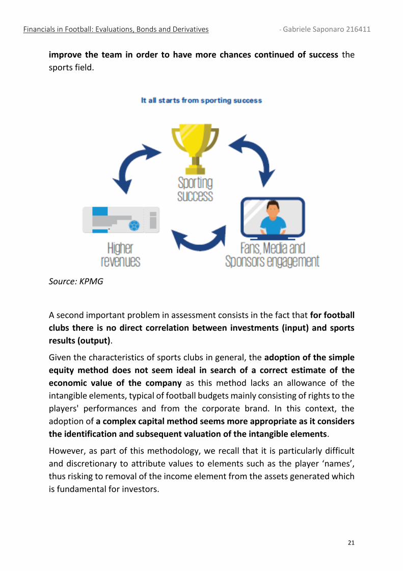
KPMG Approach In this regard, KPMG summarizes the virtuous circle that is created when a club
achieves sports success that increases the involvement of fans, media and
sponsors, which causes an increase in revenues that can in turn be used to
Financials in Football: Evaluations, Bonds and Derivatives - Gabriele Saponaro 216411
21
improve the team in order to have more chances continued of success the
sports field.
Source: KPMG
A second important problem in assessment consists in the fact that for football
clubs there is no direct correlation between investments (input) and sports
results (output).
Given the characteristics of sports clubs in general, the adoption of the simple
equity method does not seem ideal in search of a correct estimate of the
economic value of the company as this method lacks an allowance of the
intangible elements, typical of football budgets mainly consisting of rights to the
players' performances and from the corporate brand. In this context, the
adoption of a complex capital method seems more appropriate as it considers
the identification and subsequent valuation of the intangible elements.
However, as part of this methodology, we recall that it is particularly difficult
and discretionary to attribute values to elements such as the player ‘names’,
thus risking to removal of the income element from the assets generated which
is fundamental for investors.
Financials in Football: Evaluations, Bonds and Derivatives - Gabriele Saponaro 216411
22
In any case, the income methods do not seem adequate to the particularity of
the clubs, since the difficulties linked to the punctual determination of future
incomes, the choice of the discount rate as well as the historical problem of
losses in the football sector cannot be neglected. For companies in crisis in fact,
the same considerations given in the assessment for "in health" companies do
not apply first of all as regards the state of operating uncertainty in which these
companies are located.
In terms of financial methods, T. Markham in his 2013 paper, inserts the DCF
methodology among the ideal models. In his work the DCF approach is
suggested even if it presents similar difficulties to the income one due to the
lack of reliable future forecast plans (regarding the volatility of the typical
performance of the football businesses), while the valuation of the stock market
values is considered unsuitable. The latter, although they represent market
values, represent a small number of exchanges due to the lack of liquidity that
makes them subject to speculative behavior.
According to Markham himself, the multiples method of turnover is not a
reliable model of assessment for clubs, since this methodology, even if it allows
a quick sanity check of the enterprise value, is likely to lead to unsteady values
due to an underestimation of effects that the capital structure (leverage /
access to credit and related costs) could have on the ability to generate income
for the most "unbalanced" clubs from an economic-financial point of view.
Currently, however, a whole series of "hybrid" methods, based on particular
algorithms, such as those provided by various specialized companies such as
Forbes and KPMG, as well as the same soccer information provider Deloitte,
which, precisely on the evaluation of the players and their non-recourse
financing, it is also a market consolidation.
Over the years, among the various methodologies formulated and proposed, the
one used by the American specialized company Forbes has met with great
success among the insiders of the main American sports, or teams participating
in the NFL (National Football League), NBA (National Basketball Association),
NHL (National Hockey League) and MLB (Major League Baseball).
Only since 2004, following the huge follow-up achieved by the football
phenomenon in the world and the increasingly important figures that
characterized the business, Forbes thought to draw the first ranking of value in
Financials in Football: Evaluations, Bonds and Derivatives - Gabriele Saponaro 216411
23
the sector, or the 20 most valuable football teams in the world using multiples
based on sector data published by Deloitte.
Over time, Forbes has developed an algorithm that has replaced, or better
integrated, the previous traditional model focused mainly on market multiples
as summarized by Mike Ozanian (Forbes staff member): "Operating income is
earnings before interest, depreciation and amortization, player trading and
disposal of player registrations. Most Revenue figures are from Deloitte's Money
League report. "In this regard, Markham argues that "Historically, the technique
favored by Forbes in valuing clubs was based on multiples of revenue."
FORBES Approach In essence, the Forbes method breaks down the economic value of the football
companies (equity plus net debt) based on the current agreement of the
stadium (unless the new stadium is in progress) in the following four parts: i)
match day portion of the value of a club deriving from the revenues of the
various activities on the day of the match; ii) broadcasting for the portion of the
value of a club deriving from the distribution of domestic and international
television rights regarding the championship, the national cups and possibly the
international ones; iii) commercial for the portion of the value of a club deriving
from sponsorships, merchandising and revenues from other commercial
activities; iv) brand for the portion of the value of a club in excess of the sum of
the three previous parameters.
The report published by Deloitte this year and referred to the 2017/2018
financial statements shows that the revenues of the 20 football companies with
the highest turnover in the world generated revenues of € 8,3 billion, an increase
of 5% compared to the survey of last year.
All the clubs in the ranking have seen their revenues increase, which Deloitte
divides into match days, television rights and commercial revenues, compared
to the previous year. In this regard Marco Vulpiani, partner at Deloitte and
Sector Leader, states that "the British clubs record high positions in the rankings
mainly thanks to the excellent infrastructure and additional services they are
able to offer to their public. In this sense, the results of Juventus also
demonstrate how strategic it is to invest in a stadium owned by the club and in
its image and the recent rebranding of the club shows the will to continue on
this path ".
Financials in Football: Evaluations, Bonds and Derivatives - Gabriele Saponaro 216411
24
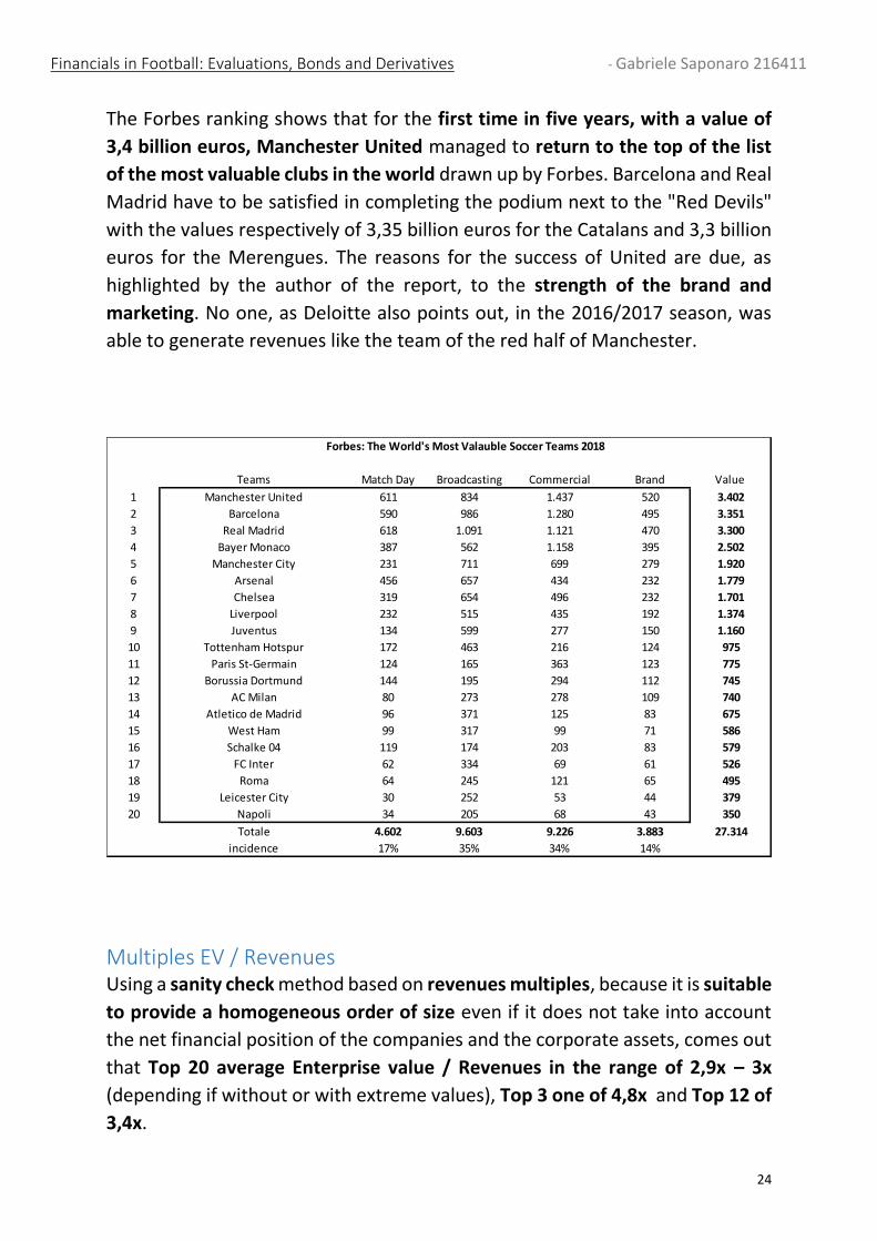
The Forbes ranking shows that for the first time in five years, with a value of
3,4 billion euros, Manchester United managed to return to the top of the list
of the most valuable clubs in the world drawn up by Forbes. Barcelona and Real
Madrid have to be satisfied in completing the podium next to the "Red Devils"
with the values respectively of 3,35 billion euros for the Catalans and 3,3 billion
euros for the Merengues. The reasons for the success of United are due, as
highlighted by the author of the report, to the strength of the brand and
marketing. No one, as Deloitte also points out, in the 2016/2017 season, was
able to generate revenues like the team of the red half of Manchester.
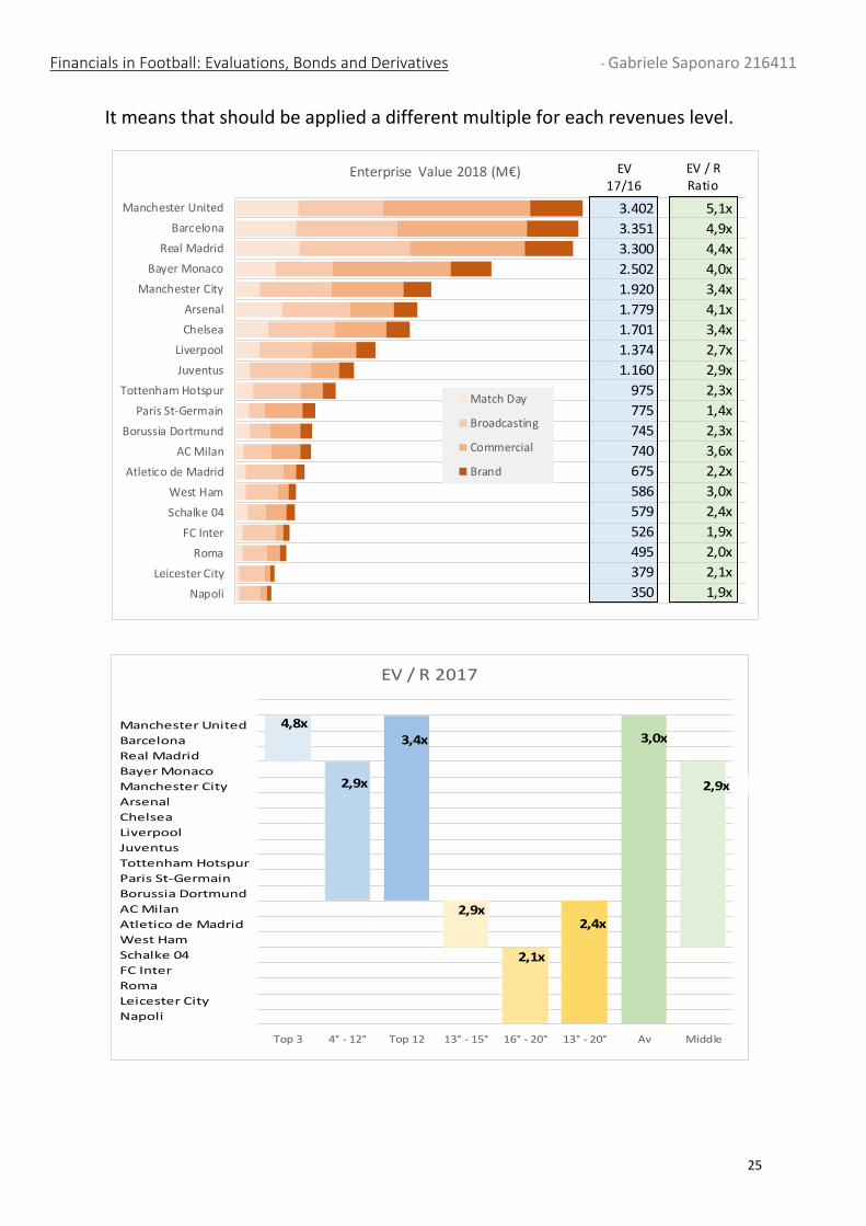
Multiples EV / Revenues Using a sanity check method based on revenues multiples, because it is suitable
to provide a homogeneous order of size even if it does not take into account
the net financial position of the companies and the corporate assets, comes out
that Top 20 average Enterprise value / Revenues in the range of 2,9x – 3x
(depending if without or with extreme values), Top 3 one of 4,8x and Top 12 of
3,4x.
Teams Match Day Broadcasting Commercial Brand Value
1 Manchester United 611 834 1.437 520 3.402
2 Barcelona 590 986 1.280 495 3.351
3 Real Madrid 618 1.091 1.121 470 3.300
4 Bayer Monaco 387 562 1.158 395 2.502
5 Manchester City 231 711 699 279 1.920
6 Arsenal 456 657 434 232 1.779
7 Chelsea 319 654 496 232 1.701
8 Liverpool 232 515 435 192 1.374
9 Juventus 134 599 277 150 1.160
10 Tottenham Hotspur 172 463 216 124 975
11 Paris St-Germain 124 165 363 123 775
12 Borussia Dortmund 144 195 294 112 745
13 AC Milan 80 273 278 109 740
14 Atletico de Madrid 96 371 125 83 675
15 West Ham 99 317 99 71 586
16 Schalke 04 119 174 203 83 579
17 FC Inter 62 334 69 61 526
18 Roma 64 245 121 65 495
19 Leicester City 30 252 53 44 379
20 Napoli 34 205 68 43 350
Totale 4.602 9.603 9.226 3.883 27.314
incidence 17% 35% 34% 14%
Forbes: The World's Most Valauble Soccer Teams 2018
Financials in Football: Evaluations, Bonds and Derivatives - Gabriele Saponaro 216411
25
It means that should be applied a different multiple for each revenues level.
Manchester United
Barcelona
Real Madrid
Bayer Monaco
Manchester City
Arsenal
Chelsea
Liverpool
Juventus
Tottenham Hotspur
Paris St-Germain
Borussia Dortmund
AC Milan
Atletico de Madrid
West Ham
Schalke 04
FC Inter
Roma
Leicester City
Napoli
Enterprise Value 2018 (M€)
Match Day
Broadcasting
Commercial
Brand
3.402
3.351
3.300
2.502
1.920
1.779
1.701
1.374
1.160
975
775
745
740
675
586
579
526
495
379
350
5,1x
4,9x
4,4x
4,0x
3,4x
4,1x
3,4x
2,7x
2,9x
2,3x
1,4x
2,3x
3,6x
2,2x
3,0x
2,4x
1,9x
2,0x
2,1x
1,9x
EV17/16
EV / RRatio
Top 3 4° - 12° Top 12 13° - 15° 16° - 20° 13° - 20° Av Middle
EV / R 2017
4,8x
2,9x
3,4x
2,9x
2,1x
2,4x
3,0x
2,9x
Manchester United
Barcelona
Real Madrid
Bayer Monaco
Manchester City
Arsenal
Chelsea
Liverpool
Juventus
Tottenham Hotspur
Paris St-Germain
Borussia Dortmund
AC Milan
Atletico de Madrid
West Ham
Schalke 04
FC Inter
Roma
Leicester City
Napoli
Financials in Football: Evaluations, Bonds and Derivatives - Gabriele Saponaro 216411
26
In addition to the methodology proposed by Forbes, the KPMG network also
offers through its annual report "Football clubs' valuation - The European Elite
2017" the measurement of the economic value of the most important football
clubs in Europe. For the same KPMG analysts, the simple application of the
revenue multiple method is however considered too simplistic to be adopted
for all clubs due to differences in the markets in which they operate, revenues
from television rights and their distribution or at the level of competitiveness.
KPMG has also developed its own algorithm based on five P parameters typical
of the football industry, with different weight and meaning:
1. profitability related to the ratio of personnel costs over the last two years
compared to revenues.
2. popularity, given the strong correlation between sports successes and the
involvement of media and fans considered as followers on social media
(Instagram, Facebook and Twitter) as a good indicator of popularity.
3. sports potential (including players' property) and performance
expectations as a driver of revenue generation in commercial terms,
match days and television rights.
4. League TV property rights and their redistribution method as a key factor
in the potential revenues of a football club.
5. property of the stadium which, together with the players, represents one
of the most important activities for generating revenues.
The results of this report show that the value of the 32 major clubs in Europe
has grown, marking a significant + 14% compared to the 2016 survey. In this
regard, Andrea Sartori, KPMG's global head of sports and author of the report,
states: "The aggregate value of the 32 major European football clubs has
increased in the last year by more than 3 billion euros, a clear indicator of the
fact that the overall value of football, as a sector, has increased.
This growth is explained by the boom in football matches on pay-tv, following
the internationalization of the commercial operations of the clubs, but above
all thanks to investments in private and modern stadia and following the
adoption of more sustainable management practices ".
As for the ranking, you can see how Manchester United is considered, in front
of the Spanish Real Madrid and Barcelona that are held respectively at 2,97 and
Financials in Football: Evaluations, Bonds and Derivatives - Gabriele Saponaro 216411
27
2,75 billion euros, the club with the highest economic value, exceeding for the
first time ever the threshold of 3 billion euros.
Even here, as in previous rankings, the British are the boss by placing six of the
top ten places. Italy is still very far from the top and only places Juventus in the
top 10. AC Milan (fifteenth), AS Roma (eighteenth), FC Internazionale
(nineteenth), Napoli (twentieth) and SS Lazio (twenty-ninth) are the other
Italians present in the ranking. With regards to Italian football, Andrea Sartori
underlines how in Italy: "Juventus are the club for which sports performance is
strictly related to the trend in revenues and business value. It is also interesting
to note that the value of Juventus (€ 1.2 billion) is higher than the sum of Milan
(€ 547 million), Inter (€ 429 million) and Lazio (€ 227 million). "
Also from the differences in the various assessments which, even if they lead to
substantially similar results, are based on different methodologies, it is clear
that for the football companies the process of determining the value is far from
simple multiples. They are based on Deloitte data necessary for multiples but
also implying adjustments into so-called hybrid models formulated by Forbes,
and only two years ago, by KPMG.
To help understand the similarities and the possible differences between the
two different evaluation algorithms proposed by the two companies it may be
useful to compare the 12 football clubs included in all the classifications dealt
with in terms of overall economic value, economic value of the respective
brands and finally of the revenues obtained.
The champion refers to the following clubs belonging to the respective national
leagues: Manchester United, Manchester City, Arsenal, Chelsea, Liverpool and
Tottenham Hotspur (Premier League), Barcelona and Real Madrid in the Spanish
Liga, Bayern Munich and Borussia Dortmund in the Bundesliga , Juventus in Serie
A and Paris St-Germain Ligue 1.
Comparison KPMG vs FORBES From a very first observation we can deduce how, for both models, the positions
in the ranking are substantially identical; the only difference lies in the
inversion of the two Spanish teams since the American study positions the
Barcelona behind Manchester United, while KPMG inserts Real Madrid. All the
remaining positions, even if with different evaluations, more or less important,
are the same for both reports.

Financials in Football: Evaluations, Bonds and Derivatives - Gabriele Saponaro 216411
28
If, when regarding positions, the rankings are almost mirrored, this is only
partially valid with reference to the economic values of all the clubs taken into
consideration. On average, the ratings of the first twelve clubs diverge 10,5%.
However, if we exclude from this calculation the average of the differences
between the last two associations (Paris Saint-Germain and Borussia
Dortmund), the difference in value of the two methods decreases to a more
acceptable 6,7%. But where does this discrepancy come from? In light of all
these considerations made, it can be said that the discrepancy is animated by
the different algorithms underlying the two evaluation models, as well as from
the weight of the various parameters within the algorithms themselves and
finally from a possible diversity of availability of the same information,
recalling that Forbes takes into account the value deriving from match days,
television rights, commercial revenues and the brand, while KPMG considers
profitability, popularity, sporting potential, television rights and finally
ownership of the stadium.
As for the valuations of Deloitte, which have taken care to estimate respectively
the value of the brand and the revenues of the various clubs, it can be stated
that they also substantially follow the positions outlined by Forbes and KPMG
with the exception of Paris Saint-Germain, who are out of the top 10 in both
classifications of overall value, while they are relatively in the seventh and sixth
place.
Financials in Football: Evaluations, Bonds and Derivatives - Gabriele Saponaro 216411
29
CHAPETR 3 - Financial Economics of Football Teams
Indexes of Football Teams The main objective of accounting analysis is to point out the financial situation
and its equilibrium through the most appropriate synthetic economic financial
indexes for the kind of business under evaluation. These indexes have to be
directly valuable for the management and a key element for their effectiveness
is their ability to compare historical results of the same company and/or results
coming from other companies active within the same business sector.
There are a number of metrics that can be used to compare clubs, including
attendance, worldwide fan base, broadcast audience, revenues and
profitability. In the Money League Deloitte focus on a club’s ability to generate
revenue from match day, broadcast rights, commercial sources (including
sponsorship, merchandising, stadium management) and extraordinary result
from buying and selling football players (indicated as components of
extraordinary management). Over and above plain vanilla analysis and
comparison among soccer companies of revenues breakdown, a first useful
business sector index is the ratio between total collection per match day
income and the number of attendances. It gives an immediate idea of
attractiveness of the team and does not require a particular accounting
reclassification and may be easily provided by the companies for an unique
comparison.
The indexes point the incidence of costs on revenues and the breakdown of
costs themselves, and are able to identify the level of efficiency of the
organization. The main principal costs typical of the management of soccer
companies, that not include real estate business itself, are related to the football
players and staff both in terms of salary as is the amortization of intangible
rights of use of professional athletic performance (players' registration rights or
right to use).
It’s necessary make clear that there exist different ways to account for the two
kind of costs related to sports performances of the players and, independently
from what has been adopted from the companies, a careful reclassification is
indispensable for a fair comparison among clubs.
Whilst for the salaries there are not doubt a question of timing for cost
recognition, there is not agreement on multi-year costs linked to right of use.
Financials in Football: Evaluations, Bonds and Derivatives - Gabriele Saponaro 216411
30
For the intangible item pertaining the right of use it is possible to record the
transaction in Profit and Losses with a full, clear, prudent and objective
adherence to the cash flow approach as well as being able to capitalize these
costs and differentiate through amortization in Profit and Losses the weight of
extraordinary transactions. Applying the second methodology it would be
possible record the value of the team in the balance sheet and in the
accompanying notes. It gives a fair representation of the team value through
periodical adjustments (increase for appreciation /decrease for depreciation
and amortization) that, according IAS principles (16,19,32), will have an impact
in both the Profit and Loss and in the Balance Sheet. Differently from the first,
according this second methodology of fair value representation, the Return on
Equity ratio would be impacted by higher return and higher asset values with an
effective market return also avoiding volatility of the index otherwise linked at
the period of the transaction.
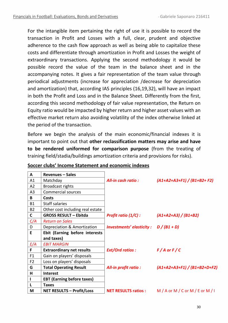
Before we begin the analysis of the main economic/financial indexes it is
important to point out that other reclassification matters may arise and have
to be rendered uniformed for comparison purpose (from the treating of
training field/stadia/buildings amortization criteria and provisions for risks).
Soccer clubs’ Income Statement and economic indexes
A Revenues – Sales
A1 Matchday All-in cash ratio : (A1+A2+A3+F1) / (B1+B2+ F2)
A2 Broadcast rights
A3 Commercial sources
B Costs
B1 Staff salaries
B2 Other cost including real estate
C GROSS RESULT – Ebitda Profit ratio (1/C) : (A1+A2+A3) / (B1+B2)
C/A Return on Sales
D Depreciation & Amortization Investments’ elasticity : D / (B1 + D)
E Ebit (Earning before interests and taxes)
E/A EBIT MARGIN
F Extraordinary net results Ext/Ord ratios : F / A or F / C
F1 Gain on players’ disposals
F2 Loss on players’ disposals
G Total Operating Result All-in profit ratio : (A1+A2+A3+F1) / (B1+B2+D+F2)
H Interest
I EBT (Earning before taxes)
L Taxes
M NET RESULTS – Profit/Loss NET RESULTS ratios : M / A or M / C or M / E or M / I
Financials in Football: Evaluations, Bonds and Derivatives - Gabriele Saponaro 216411
31
The first economic index to study and understand during a financial analysis,
independently from the business sector, is the Gross Result of ordinary
activities (excluding any atypical result from extraordinary activities as the
transaction on intangible right of use) on Revenues form typical activities. The
return on sales (also called Ebitda margin) gives an immediate perception of
acompany’s ability to make a profit form the investments spent, while
including in the costs also the amortization it is possible to obtain the net result
(Ebit) on sales (ebit margin) as an indicator of company profitability net of the
cost of its investments.
Among those economic indexes useful for a full understanding of financial
equilibrium there are those that show relations among specific positive and
negative economic items. Starting from typical operation analysis it’ common
to compare at first all revenues including collection from trading (match days
collection + commercial sources + broadcast rights + capital gain on trading) with
all costs (salaries + amortization + capital losses on trading). A second view of
the same index may be obtained removing from the index those items
pertaining to extraordinary economic components, or directly measuring the
incidence of the extraordinary components in respect of an ordinary one,
comparing capital gain/losses on trading with ordinary revenues (match days
collection + commercial sources + broadcast rights), or comparing capital
gain/losses on trading with gross margin (Ebitda).
Another useful index of operating costs able to measure the elasticity of
investments is the comparison of amortization of right of use with total costs.
In in this comparison if we decide to add also the costs for salaries then it
becomes possible understand the incidence of the overall cost afferent the
human resources on total costs.
Financial Statements as information and measure instrument The introduction of the regulation of the Financial Fair Play by the UEFA and the
scarcity of the available resources will force a rethinking of management
dynamics and will push management to planning for interventions that will not
exceed the real availability of financial resources. Inserted in this new frame of
reference, the financial statement document completes, for professional
football clubs, its transmutation from an element of pure and correct
information to a fundamental component in the business strategy.

Financials in Football: Evaluations, Bonds and Derivatives - Gabriele Saponaro 216411
32
In short, from the balance sheet, they will not only have to draw numbers and
indices, but mainly strategic directions. Investments, in particular, will have to
be oriented mainly towards the consolidation of a club’s assets. By carefully
evaluating the balance between revenues and costs, it will be possible to
operate according to sustainable sports programs in the short and medium
term. These and other key factors can be developed only if the management will
have an agile tool available in the time and immediate readability for all its users.
The latter will not only be the third parties interested in controlling an economic
and financial solidity aimed at maintaining the commitments (suppliers, other
clubs, customers or fans), but also the governing institutions in charge of
verifying regular participation in competitions.
The balance, no longer a simple best practice but a real regulatory obligation,
will be a sort navigation tool to allow management to develop projects and
programs (sports and financial) consistent with the economic balance.
The same introduction of the Financial Fair Play will require an interpretative
and adaptive effort, both by the UEFA and the National Federations, in order to
allow a uniform application within the 52 countries involved. In fact, in the
accounting and, above all, tax matters, the UEFA area is characterized by a very
high heterogeneity of the regulations in force and if this evident application
discrepancy is not exceeded, any attempt at reform risks giving way to an
extreme and prolonged conflict between the different legal jurisdictions
involved.
Case study: Real Madrid, still the team to beat? To conclude the work carried out attempts to identify a prospective trend and it
was decided to carry out the analysis of the benchmark club as excellence (Real
Madrid), which more than any other sports team results with excellent
economic-financial performance that allows it to occupy from the very first
years the top ranking position drawn up every year by Deloitte regarding clubs
by turnover.
For ReaI Madrid, considered by Forbes as a sports club with a top and stable
rating, the Merengue brand is equal to over 3 billion dollars, a technical analysis
was carried out aimed at deepening its structure of the income statement with
attention to the net financial indebtedness ratios and the break-even result. In
addition, some efficiency indicators have been explained and analysed for the

Financials in Football: Evaluations, Bonds and Derivatives - Gabriele Saponaro 216411
33
Galatticos, including the total solvency index, the indebtedness index, the net
financial position and the cost of employees.
Operating revenues, excluding the gains on the sale of players, amounted in
17/18 to € 750 million, also for preceding year, placing itself first in the world
since 2011/12 and constantly above the threshold of € 500 million, representing
the amount of sector revenues as being the highest in the world.
The sources of revenue (match days, television rights and marketing) have
historically been fairly distributed (30% of revenues from ticketing and
118 119 114 130 129 136 143186 188 204 200 228 237 251
210 212 232 247 263301
356
513 519 550 577620
674750
0
100
200
300
400
500
600
700
800
11/12 12/13 13/14 14/15 15/16 16/17 17/18
Real Madrid revenues evolution (euro millions) dand cagr 2011/12 - 2017/18
MATCHDAYS: 3,3% BROADCAST: 5,1% COMMERCIAL: 9,2% TOTAL REVENUES: 6,5%
9%
0%
13%
11%
7%
3%
5%
9%
6%
3%3%
11%
0%
2%
4%
6%
8%
10%
12%
14%
Total revenues Matchdays: 3,3% Broadcast: 5,1% Commercial: 9,2%
Cagr 11/12 - 17/18
Manchester United Real Madrid FC Barcelona
Financials in Football: Evaluations, Bonds and Derivatives - Gabriele Saponaro 216411
34
membership fees, 30% from television rights and 40% from trade revenues
which have increased significantly compared with the past). The average annual
growth rate is 10% and the diversification of sources confers economic stability,
mitigating the impact of any fluctuations caused by sporting results or other
cyclical causes.
The cost of personnel amounts to approximately 300 million euros and, if
compared to operating income excluding capital gains, determines a value of
50% of the indicator used internationally to measure the operating efficiency of
football clubs. The maximum level recommended by the European Club
Association is 70%, thus we can appreciate how the Madrid club is considered
to be of excellence within the sector. It therefore follows that Real Madrid can
afford a squad of football players with a high level of income because its
economic management generates an equally high turnover. EBITDA, is the gross
result before the calculation of depreciation and interest and taxes, again with
the exclusion of the minus / capital gains, amounts to approximately 250
millions euros, while the pre-tax result amounts to approximately 150 millions
euros and a lows it to comply with the set breakeven result parameters
according to which the cumulative sum of the last three years cannot be lower
than a certain defined year-on-year threshold (also negative as cumulative loss).
Basically according to the financial fair play the important thing is that you do
not spend more than your receipts, but in the case of the Real Madrid Polis port
which also includes other sports with a negative result, the breakeven of the
football sector must also offset the results of the other disciplines sports.
The Debt / Ebitda ratio is one of the most used indicators of the credit market
as it provides an approximate idea of how many years is necessary for the
company to be able to repay its net financial debt. Obviously, it is an indicator
whose sustainability is closely linked to the predictability and certainty over time
of the operating financial flows that the company is able to produce and markets
with high uncertainty will allow debt with a low multiples while others are more
stable and will allow higher multiples. The football sector has multiples ranging
from 2 to 3 and Real Madrid underlines its financial strength with a multiple of
only 0,5. That proves that, if managed professionally, the football sector is highly
remunerative and does is one which doesn’t require the use of huge amounts of
capital (and indebtedness) if over the years one is able to generate cash flows
capable of repaying and remunerating the capital invested.
Financials in Football: Evaluations, Bonds and Derivatives - Gabriele Saponaro 216411
35
The debt must be sustainable and the same financial fair play requires that there
are no problems related to expired debts towards other clubs, tax authorities
and their employees (with the exception of those for bonuses not yet achieved).
While the debt ratio equal to the ratio between shareholders' equity and total
liabilities is equal to 0.67 which implies 40/60 covered loans between equity and
total indebtedness, the D / E ratio between net financial indebtedness and net
equity for Real Madrid it is equal to about 0,25 (net financial indebtedness equal
to a quarter of the means) which means that the resources (PN / CIN equal to
about 80%) fund a large part of the net invested capital.
The equity, which according to the financial fair play must be non-negative and
growing, amounts to over 400 million euro and therefore the total assets, are
estimated to be more than one billion euro.
The solvency ratio is equal to the ratio between total assets and total debts and
is 1,7 million for Real Madrid, which means that the Merengues are solvent since
their asset value can fully cover (if = 1) and over (> 1) of their total debt.
Specifically, we note that the component of the most risky assets relating to
players' registration rights, if compared to shareholders' equity, results less than
90%, proving that even an unlikely complete devaluation of the entire player
park would not jeopardize the ability of Real Madrid to repay its debts and
partially absorb the equity. Finally, it is worth noting in terms of the evolution of
investments that the Madrid club has invested over 300 million euros in the last
decade on its stadium and the modernization of the facilities to improve its
functionality and consequently creating a very significant economic return.
Financially everything seems perfect, but is it enough?
The rights accrued with the victory of the 2018 Champions League that will be
brought in the next few years will certainly return to compete for the Deloitte
Money League Real for next season but at the same time the sale of CR7 after 8
years of his role in the growth of Real, despite being an extraordinary income
activity that does not directly affect the revenues considered by the Deloitte
Money League, would probably have a catastrophic effect not only on followers,
but also on merchandising and television rights that will make the results of the
ranking in the next few years more unpredictable, giving a boost to Juventus.
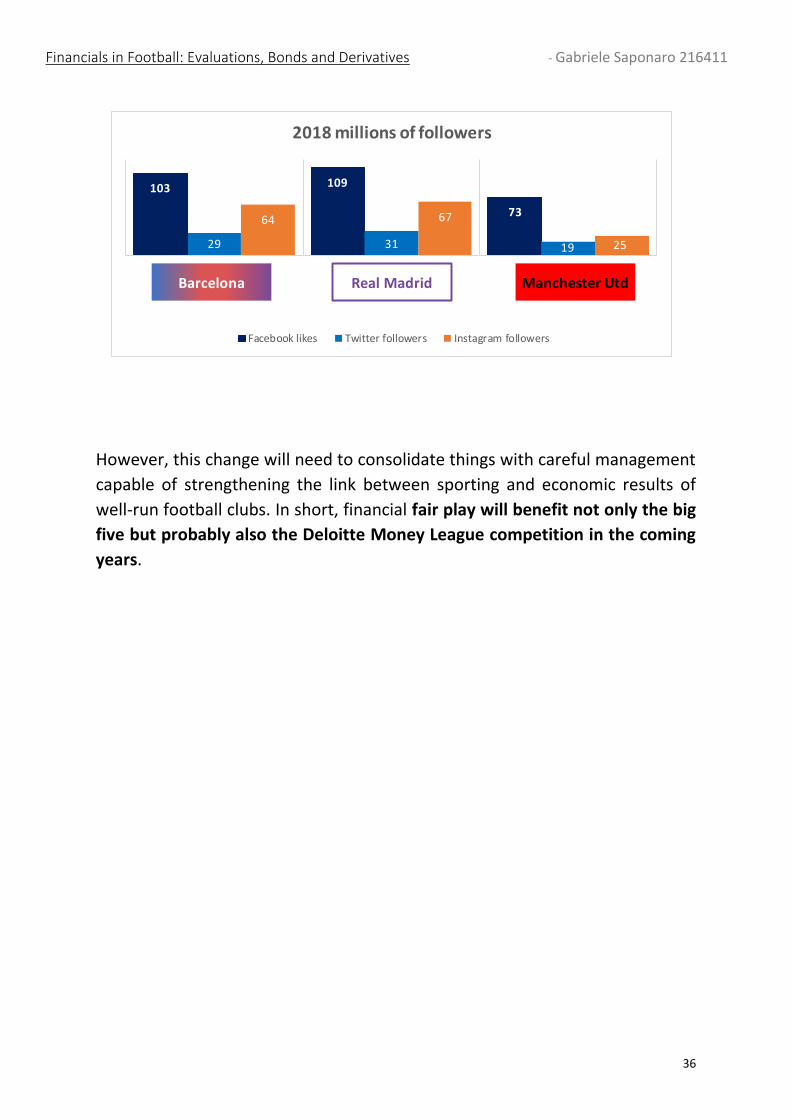
Financials in Football: Evaluations, Bonds and Derivatives - Gabriele Saponaro 216411
36
However, this change will need to consolidate things with careful management
capable of strengthening the link between sporting and economic results of
well-run football clubs. In short, financial fair play will benefit not only the big
five but probably also the Deloitte Money League competition in the coming
years.
103 109
73
29 31 19
64 67
25
FC Barcelona Real Madrid Manchester United
2018 millions of followers
Facebook likes Twitter followers Instagram followers
Barcelona Real Madrid Manchester Utd
Financials in Football: Evaluations, Bonds and Derivatives - Gabriele Saponaro 216411
37
CHAPTER 4 - IAS 39 and IFRS 9
SCOPE OF APPLICATION of IAS 39 The purpose of this principle is to establish the criteria for the detection,
evaluation and disclosure relating to financial instruments in the financial
statements of companies.
Football teams have their assets value “limited” by international accounting
standards, but using specific financial contracts there can be an assets value
increase due to IAS 39 principle.
In fact, the objective of IAS 39 is to define the principles for the recognition and
measurement of financial instruments.
A financial instrument is a contract resulting in a financial asset for one company
and an equal financial liability (or equity instrument) for another company.
While a financial asset may consist of: cash, contractual rights to receive cash or
another financial asset from another enterprise, contractual rights to exchange
financial instruments with another enterprise under potentially favourable
conditions or equity instrument of another company, a financial liability is a
contractual obligation to deliver cash or another financial asset to another
enterprise or to exchange financial instruments with another enterprise under
potentially unfavourable conditions.
Particular financial instruments are derivatives, that are characterized by:
(a) Value changes in relation to changes that occur on a predetermined
“underlying”, as can be football players value, that may either be interest rate,
price of a security, price of a commodity, exchange rate in foreign currency,
index of prices or rates, credit rating,
(b) Which requires no initial net investment or a minimum initial net investment
relating to other types of contracts which have a similar reaction to changes in
market conditions;
(c) Which will be settled in the future.
IAS 39 requires that all financial assets and financial liabilities are recognized
in the financial statements. This also applies to all derivative contracts.
Initially a financial asset or financial liability is recognized for the first time in the
financial statements as a cost, which is also equal to the fair value of the
Financials in Football: Evaluations, Bonds and Derivatives - Gabriele Saponaro 216411
38
consideration given in exchange (in the case of an asset) or received (in the case
of a liability).
Financial assets can be classified into four categories:
1) loans and receivables originated by the company and not held for negotiation;
2) investments held to maturity;
3) financial assets available for sale;
4) financial assets held for trading
Subsequently the financial instruments are valued at fair value or at amortized
cost, according to the category in which they are classified
As with the other IAS, the scope is defined with an exclusion procedure. The
following financial instruments are excluded from the application of this
principle:
1) Equity investments in subsidiaries, associates and companies subject to joint
control, to which IAS 27, 28 and 31 apply;
2) Rights and obligations deriving from leasing contracts, to which IAS 17 applies;
3) Assets and liabilities held by an employer and tied to a pension plan, at which
IAS 19 applies;
4) Rights and obligations contained in insurance contracts.
However IAS 39 does apply to in insurance derivatives incorporated contracts;
equity instruments, including warrants, options and other instruments,
classified by the issuer among the components of equity. This means that IAS 39
must apply to these instruments:
1) Financial guarantee agreements, such as sureties, letters of credit, which
provide for payments to be made in the event of default by the principal;
2) Contracts concerning price adjustments on the sale of companies; contracts
that prescribe payments related to climatic, geological or other variables
IAS 39 applies, therefore, to the following financial instruments:
Debt titles;
Equity securities (except for investments in subsidiaries, associates and
joint ventures);
Financials in Football: Evaluations, Bonds and Derivatives - Gabriele Saponaro 216411
39
Other financial assets, such as investments and credits (whether they
"originated" from the company or "acquired" from other companies);
Financial liabilities (whether they "originated" from the company or
"acquired" from other companies);
Financial derivative instruments (be they derivative assets or liabilities);
Derivative financial instruments ("embedded") in other financial
instruments;
Assets and liabilities used as hedging instruments.
Of particular importance is the fact that IAS 39 provides for the recognition in
the financial statements of all derivative instruments while today these
instruments are often not recognized.
The definitions contained in IAS 39 are indispensable for understanding the
entire Standard. With regard to financial instruments, IAS 39 provides the
following fundamental definitions:
Financial instrument is any contract that gives rise to a financial asset for a
company and to a financial liability or a representative instrument for another
company.
Financial activity is any activity that is; cash and cash equivalents, a contractual
right to receive cash or another financial asset from another enterprise, a
contractual right to exchange financial instruments with another enterprise on
potentially favourable terms; or an equity instrument of another company.
Financial liability is any liability that is a contractual obligation to deliver cash or
another financial asset to another enterprise, or to exchange financial
instruments with another enterprise under potentially unfavourable conditions.
Equity instrument is any contract that represents a residual investment in the
assets of a company net of all its liabilities, that is, an equity investment.
Financial derivative instrument is a financial instrument whose value changes
in relation to changes that occur in a predetermined interest rate, price of a
security, price of a commodity, exchange rate in foreign currency, index of prices
or rates, credit rating or other variable (sometimes called "underlying"), which
requires that there is no initial net investment or a minimum initial net
investment relating to other types of contracts which have a similar reaction to
changes in market conditions and which will be settled in the future.
Financials in Football: Evaluations, Bonds and Derivatives - Gabriele Saponaro 216411
40
For the application of the above definitions, another accounting principle (IAS
32) states that the term "enterprise", that is is inclusive of natural persons,
partnerships, legal entities and public bodies.
In IAS 39 the financial instruments defined above are classified into four
categories, to which different valuation criteria apply. The definitions of the four
categories below are therefore fundamental for fully understanding IAS 39.
The four categories identified are:
1. Financial asset or liability held for trading
Financial instruments fall into this category when a financial asset was
purchased or a financial liability was incurred primarily for the purpose of
generating a profit from short-term price fluctuations or margin of profit of
the operator.
A financial asset must be classified as held to be negotiated if, regardless of
the reason for which it was purchased, it is part of a portfolio for which
there is evidence of recent and effective manifestation of a profit
realization in the short term.
According to IAS 39, derivative financial instruments (be they derivative
assets or derivative liabilities) are always held to be traded unless they are
designated and are effective as hedging instruments.
2. Investments held to maturity
They are financial assets with fixed or determinable payments and fixed
maturity that a company has the actual intention and ability to possess to
maturity with the exception of the loans and credits originated by the
company, which constitute a category apart from.
3. Loans and receivables originating from the company:
They are financial assets that are created by the company by supplying
money, goods or services directly to a debtor, with the exception of those
that originated with the intention of being sold immediately or in the short
term, which they must be classified as owned to be negotiated. Loans and
receivables originating from the company are not included among the
investments held to maturity but, rather, are classified separately
according to the provisions of this Standard.
4. Financial assets available for sale
Is a residual category that includes financial assets that are not:
(a) Financial assets held for trading.
Financials in Football: Evaluations, Bonds and Derivatives - Gabriele Saponaro 216411
41
(b) Investments held to maturity, or
(c) Loans and receivables originating from the company.
Recognition and measurement of financial instruments The definitions provided by IAS 39 are as follows:
Fair value: is the consideration at which an asset can be exchanged, or an
extinguished liability, between aware and available parties, in a fair transaction.
Amortized cost of a financial asset or liability: is the value at which the financial
asset or liability was valued upon initial recognition net of principal repayments,
increased or decreased by the overall amortization of the differences between
the initial value and that at maturity, and net of any write-down (made directly
or through the use of a fund) following a lasting reduction in value or insolvency.
Effective interest criterion: it is a criterion for calculating amortization based on
the use of the effective interest rate of a financial asset or liability. The effective
interest rate is a rate that accurately discounts the expected flow of future cash
payments up to the expiration date or the next date of recalculation of the price
based on market value, so as to obtain the current net book value of the asset
or financial liability. This calculation must include all fees and points paid or
received between the parties involved in the contract. The effective interest rate
is sometimes qualified as the level of return on maturity or on the next price
recalculation date, and is the internal rate of return on the asset or liability in
that year.
IAS 39 provides rules for the accounting of financial instruments used to hedge
other assets and liabilities. Hedging for accounting purposes, it means
designating one or more hedging instruments, so that their changes in fair value
lead to offsetting, in whole or in part, of the change in fair value or the cash flows
of a hedged item.
An hedged item is an asset, liability, irrevocable commitment, or expected
future transaction that exposes the company to the risk of changes in fair value
or future cash flows, and which for hedge accounting purposes, is designated as
a hedge.
On the other hand hedging instrument is a designated derivative or (in limited
circumstances) another financial asset or liability whose fair value or cash flows
are expected to offset changes in fair value or cash flows of a designated covered
Financials in Football: Evaluations, Bonds and Derivatives - Gabriele Saponaro 216411
42
element. According to the provisions of IAS 39, a non-derivative financial asset
or liability can be designated as a hedging instrument for hedge accounting
purposes only if it hedges the risk of changes in foreign exchange rates.
To value the efficiency of the hedging strategy we use the Hedging effectiveness
level that is the level at which compensation for changes in fair value or cash
flows attributable to a hedged risk is obtained from the hedging instrument.
DETECTION OF FINANCIALS
An enterprise must recognize a financial asset or liability in its balance sheet
when, and only when, the enterprise itself becomes a party to the contractual
clauses of the instrument. As a consequence of the foregoing, an enterprise
recognizes all contractual rights and obligations arising from derivative contracts
as assets or liabilities in its balance sheet.
DATE OF NEGOTIATION / DATE OF REGULATION
A "regular" purchase or sale 2 of financial assets must be recognized using:
accounting at the settlement date method. The method used must be applied
consistently for all purchases and sales belonging to the same category (assets
/ liabilities held to be negotiated; investments held to maturity; loans and
receivables originated by the company; financial assets available for sale).
The negotiation date is the date on which an enterprise undertakes to buy or
sell an asset. Accounting on the trade date refer to the recognition of the asset
that must be received and the liability that must be paid on the date of
negotiation; or the elimination of an asset sold and the recognition of a credit
towards the buyer for payment on the negotiation date.
The settlement date is the date on which an activity is delivered to the company
or by a company, which implies the detection of an asset on the day it is
transferred to an enterprise; the elimination of an activity on the day it is
transferred from the company.
In the case of accounting at the settlement date, the company will record - in
the period between the negotiation date and the settlement date - any change
in the fair value of the asset.
Financials in Football: Evaluations, Bonds and Derivatives - Gabriele Saponaro 216411
43
ELIMINATION or TRANSFER
A company must reverse a financial asset when it loses control of the contractual
rights represented by that asset. Control is lost when the company exercises or
collects the rights or benefits under the contract, the rights expire, or the
company transfers these rights.
The determination of the loss of control over a financial asset by an enterprise
depends on the position of the enterprise or that of the assignee. If the position
of both companies indicates that the transferor has maintained control, they
must not remove the asset from its balance sheet.
When the assignee has the right to repurchase the asset at a predetermined
price that could be different from the current value, or there are call options for
the assignor and put options for the assignee with substantially similar exercise
price, there is no loss of control. The transferor generally loses control of the
business when the transferee is able to obtain the benefits associated with the
property by selling or pledging the business.
SOME SPECIAL CASES
a) Partial transfer of a financial asset, that happens if one company transfers to
another a part of a financial asset, while retaining ownership of the rest, then
the book value of the financial asset must be divided between the asset sold and
that maintained based on their current value relating to the date of the sale.
b) Sale of assets associated with new financial assets or liabilities occurs if a
company transfers a financial asset and simultaneously creates a new financial
asset or assumes a liability, it will have to account for the current value of the
new asset or liability and will also have to account for the profit o the loss
deriving from the transaction as the difference between the consideration and
the current value of the asset sold plus the current value of the new liability
assumed less the current value of the new asset acquired more or less any value
adjustments that had previously been accounted for in equity.
c) A company will eliminate a financial liability (or part of it) from its balance
sheet only when it is extinguished, that is, after the fulfilment, cancellation or
expiry of the contractual obligation.
The replacement between an existing debtor and his lender of debt instruments
under substantially different conditions is an extinction of the old debt, which
Financials in Football: Evaluations, Bonds and Derivatives - Gabriele Saponaro 216411
44
should result in the elimination of that debt and the accounting of the new one.
Even a substantial change in the conditions of an existing debt instrument
should be accounted for as an extinction of the old debt.
If the replacement or modification of the terms of a debt instrument entails the
payment of commissions or other costs, these must be accounted for as part
of the profits or losses on the payments. If the contractual changes are not
accounted for as debt settlement, the costs and commissions are adjustments
to the book value of the liabilities and must be amortized over the remaining
term of the loan.
The contractual conditions are substantially different if the present value of the
cash flows envisaged by the new contract, including the costs paid and net of
any commissions collected, differs by at least 10% from the present value of the
residual cash flows envisaged by the contract native to.
The difference between the amount paid for the elimination or transfer of a
liability and its book value must be included in the result of the year. Partial
elimination of a liability or elimination associated with new financial assets or
liabilities The elimination of partial liabilities or associated with the creation of
new assets or liabilities is accounted for as the corresponding transactions
connected with the total or partial elimination of assets.
EVALUATION INITIAL ASSESSMENT OF ACTIVITIES AND FINANCIAL LIABILITIES
When a financial asset or financial liability is recognized for the first time, an
enterprise must evaluate it at cost, or at the fair value of the consideration given
in exchange (in the case of an asset) or received (in the case of a liability).
Transaction costs are included in the initial recognition of all financial assets and
liabilities.
The fair value of the consideration given or received can normally be determined
by referring to the cost of the transaction itself or to other market values. If
these market values cannot be reliably determined, the fair value of the
consideration is estimated as the sum of all future cash payments or
collections, discounted, if the effect of discounting is significant, using the
prevailing interest rates in the market for a similar instrument (similar in
Financials in Football: Evaluations, Bonds and Derivatives - Gabriele Saponaro 216411
45
currency, in contractual terms, in the type of interest rate and other factors) of
an issuer with a similar credit rating.
SUBSEQUENT ASSESSMENT OF FINANCIAL ACTIVITIES
For the purpose of evaluating a financial asset subsequent to initial recognition,
this Standard classifies financial assets into different categories:
1) Loans and credits originated by the company and not held for negotiation;
investments held to maturity;
2) Financial assets available for sale;
3) Financial assets held for trading.
After initial recognition, an enterprise must evaluate financial assets, including
derivatives that constitute financial assets, at their fair value, without any
deduction for the transaction costs that may be incurred in the sale or other
disposal, except for loans and credits originated by the company and not held
for negotiation, investments held to maturity, any financial asset that does not
have a market price listed on an active market and whose fair value cannot be
reliably determined.
These financial assets must be valued on the basis of the amortized cost
criterion. However, fair value is a more appropriate method of measuring the
amortized cost for most financial assets. To fully understand the fair value
principle we also have to dig in the amortized cost and the problems connected
with holding the investments until maturity.
THE FAIR VALUE
The fair value can be reliably determined for most of the financial assets
classified as available for sale or held for trading.
The fair value of a financial instrument can be measured reliably if and only if,
the variability in the range of reasonable fair value estimates is not wide for this
instrument, if the probabilities of the various estimates within the range can be
reasonably and is valued and used in the estimate of fair value.
The situations in which the fair value can be measured reliably include a financial
instrument for which a public price quotation exists in an active publicly
accessible securities market for that instrument, or a representative debt
Financials in Football: Evaluations, Bonds and Derivatives - Gabriele Saponaro 216411
46
instrument that has been rated by an independent rating agency and whose
cash flows can be reasonably estimated, or even a financial instrument for which
there is an appropriate valuation model and for which the input information in
this model can be reliably valued since the data come from active markets.
The fair value of a financial asset or financial liability can be determined using
one of the many generally accepted methods. The valuation techniques must
incorporate the assumptions that would be formulated in the fair value
estimates by those who participate in the market, including the assumptions
made regarding advance payment rates, presumed credit loss rates and interest
and discount rates.
Underlying the definition of fair value there is the presumption that the
company is in operation and that it has no intention or need to liquidate,
significantly reduce the scope of its activities or undertake an operation under
unfavourable conditions.
The existence of public price quotations in an active market is usually the best
indication of fair value. The most appropriate price quoted on the market for
an asset held or a liability that must be issued is the current bid price (bid)
while for an asset that must be purchased or for a liability held is the current
offer or the asking price (offer). When bid and offer prices are not available, the
price of the most recent transaction can provide an indication of the current fair
value, assuming that there have been no significant changes in the economic
circumstances between the date of the transaction and the date of allocation in
balance.
If the market for a financial instrument is not an active market, public price
quotes may need to be adjusted to arrive at a reliable fair value measurement.
If market movements are not frequent, the market is not very stable or only
small volumes are exchanged compared to the units in circulation of the
financial instrument that must be valued, the listed market prices may not be
indicative of the fair value of the instrument.
If there is no market price for a financial instrument as a whole but there are
markets for the parts that make it up, the fair value is obtained on the basis of
the relevant market prices. If there is no market for a particular financial
instrument but there is a market for such a financial instrument, the fair value is
obtained on the basis of the market price of the similar financial instrument.
Financials in Football: Evaluations, Bonds and Derivatives - Gabriele Saponaro 216411
47
There are many situations in addition to those listed in the previous points
where it is likely that the variability in the range of reasonable fair value
estimates is not significant. Normally, the fair value of a financial asset that a
company has purchased can be estimated by third parties. It is not it is likely that
a company purchases a financial instrument for which it does not believe it can
obtain a reliable fair value measurement after the purchase.
Gains and losses deriving from fair value measurement
A recognized gain or loss resulting from a change in the fair value of a financial
asset or financial liability that is not part of a hedging relationship must be
recognized in the financial statements either a profit or loss on a financial asset
or financial liability held for trading must be included in the income statement
of the year in which it occurred, or an income or expense on a financial asset
available for sale must be included in the income statement of the year in which
it occurs and recognized directly in equity, through the statement of changes in
equity.
If an enterprise recognizes the purchases of financial assets using the accounting
on the settlement date, any change in the fair value of the asset that must be
received in the period between the negotiation date and the settlement date is
not recognized for the assets entered on the cost or at amortized cost. For assets
revalued at fair value, however, the change in fair value must be recognized in
the income statement or in equity, depending on how it is most appropriate.
THE AMORTIZED COST
Those financial assets that are excluded from fair value measurement and have
a predetermined maturity must be measured at amortized cost using the
effective interest rate criterion.
Those that do not have a fixed deadline must be valued at cost. All financial
assets are subject to review to check whether there has been a lasting loss in
value.
Some examples might be, short-term loans without a pre-established interest
rate are normally valued at their original value unless the effect of imputing the
interest is significant; or loans and credit originated by a firm cannot be
negotiated are valued at their amortized cost regardless of the firm's intention
to own them until their maturity.
Financials in Football: Evaluations, Bonds and Derivatives - Gabriele Saponaro 216411
48
For variable rate financial instruments, the periodic estimate of the financial
flows that can be determined to reflect the changes in interest rates on the
market changes the effective return of a monetary financial asset. These
changes in cash flows are recognized over the residual duration of the asset, or
until the next price revision date if the asset is subject to price change (reprising).
In the case of a variable rate financial asset initially recognized at a value
equivalent to the repayable principal at maturity, re-estimating future interest
on payments normally has no significant effect on the book value of the asset.
INVESTMENTS HELD TO MATURITY
An enterprise does not have the actual intention of owning an investment in an
asset to maturity financial with a fixed maturity if one of the following conditions
is present:
1) The enterprise intends to own the financial asset for an undefined period
only;
2) The company is ready to sell the financial asset (except in the event of a non-
recurring situation that could not reasonably have been foreseen by the
company) following changes in interest rates or market risks, liquidity needs,
changes in the availability and return of alternative investments, changes in
sources and terms of financing or changes in risk on foreign currency;
3) The issuer has the right to extinguish the financial asset at an amount
significantly lower than its amortized cost.
An enterprise must not classify any financial asset as held to maturity if the
enterprise has sold, transferred or exercised a sale option during the current
financial year or the previous two for an amount which is not exactly
insignificant. Held to maturity prior to maturity (not insignificant in relation to
the overall portfolio held to maturity), except if sales fairly close to the
expiration or exercise date of any call option sold, so that changes in market
interest rates did not have a significant effect on the fair value of the financial
asset; or sales after the company has already collected substantially all the
original capital of the financial asset through ordinary scheduled or advance
payments; or sales due to an event isolated beyond the control of the company
and which is non-recurring and may not have been reasonably foreseen in
advance by the company.
Financials in Football: Evaluations, Bonds and Derivatives - Gabriele Saponaro 216411
49
On the contrary, most equity securities cannot be considered an investment
held to maturity or because it does not have a limited life span (such as, for
example, ordinary shares) or because the amounts that the owner can receive
may vary in a non-predetermined method (such as, for example, options,
warrants and rights on shares).
An enterprise is not in a position to possess an investment in a financial asset
with a fixed maturity to maturity if has no financial resources available to
continue to support the investment to maturity, and is subject to legal,
supervisory or other constraints that prevent it from holding the financial asset
to maturity.
A company must assess its intention and ability to own its investments until
maturity at each balance sheet date and classified as held to maturity until
maturity not only when such financial assets are purchased but also at each
balance sheet date.
If, following a change in intention or capacity, it is no longer appropriate to
record an investment held to maturity at amortized cost, this must be re-
evaluated at fair value, or if it becomes possible to reliably measure a financial
asset, the asset must be measured at fair value.
SUBSEQUENT ASSESSMENT OF FINANCIAL LIABILITIES
After the initial evaluation, a company must evaluate all financial liabilities
depending on the asset type.
Derivative liabilities which are connected to an unlisted equity instrument and
which must be settled with the delivery of the same instrument whose fair value
cannot be reliably measured at cost and liabilities held for trading and
derivatives which are liabilities valued at fair value.
On the other hand the financial liabilities which are designated as hedged items
valued on the basis of the provisions on hedge accounting contained in the
paragraphs relating to the hedges of this standard, while all remaining liabilities
at amortized cost.
Financials in Football: Evaluations, Bonds and Derivatives - Gabriele Saponaro 216411
50
DURABLE LOSSES OF VALUE AND IRRECUPERABILITY OF ACTIVITIES
A financial asset has suffered a lasting loss of value if its book value is greater
than its presumed realizable value. An enterprise must determine at each
balance sheet date whether there is any objective indication that a financial
asset or group of assets may have suffered a lasting reduction in value.
The objective evidence that a financial asset or group of assets has suffered a
permanent loss of value or is unrecoverable, includes information that reaches
the attention of the owner of the asset about the following points:
a) Significant financial difficulties of the issuer;
b) An effective breach of the contract, such as a default or failure to pay interest
or principal;
c) The extension from the lender to the debtor for economic or legal reasons
relating to the financial difficulty of the beneficiary, of a concession that the
lender would not otherwise have considered;
d) A high probability of bankruptcy or other financial reorganization of the
issuer;
e) The recognition of a lasting loss of value on that activity that occurred in a
previous year;
f) The disappearance of an active market for that financial asset due to financial
difficulties;
g) A historical trend of collections of receivables from customers indicative of
the fact that the full nominal amount of a portfolio of such receivables will not
be recovered.
The disappearance of an active market, due to the fact that a company's
securities are no longer publicly traded, is not evidence of a lasting loss of value.
A downgrade in the creditworthiness of a company does not in itself constitute
evidence of a lasting loss of value, although this may be indicative of a lasting
loss of value if considered together with other available knowledge.
If it is probable that an enterprise will not be able to recover all the amounts
due (principal and interest) according to the contractual agreements for
financing, credit or investments held to maturity recorded at amortized cost, it
means that there has been a lasting loss of value or a bad debt loss. The
amount of the loss is represented by the difference between the book value of
Financials in Football: Evaluations, Bonds and Derivatives - Gabriele Saponaro 216411
51
the asset and the present value of the expected future cash flows discounted at
the original effective interest rate of the financial instrument (realizable value).
Cash flows relating to short-term loans are generally not discounted. The book
value of the asset must be reduced to its presumed realization value directly or
through the use of a fund. The amount of the loss must be recognized in the
income statement for the year.
The permanent loss of value and the loss due to non-collection can be
individually assessed and recognized for financial assets that are individually
significant. The permanent loss of value and the loss due to non-collection can
be assessed and recognized on the basis of a portfolio of similar financial assets.
A lasting loss in value of a financial asset recognized at amortized cost is
measured using the original effective interest rate of the financial instrument
since discounting at the current market interest rate would, in effect, require
the fair value measurement for those assets that this Standard would otherwise
evaluate at amortized cost. If a loan, credit or investment held to maturity has
a variable interest rate, the discounting rate for assessing the realizable value
is the effective current interest rate determined according to the contract. As
a substitute calculation of fair value, a creditor can evaluate the permanent loss
of value based on the fair value of an instrument using a detectable market
price. If an asset is pledged as collateral and is likely to be foreclosed, then the
holder assesses the permanent loss of value based on the fair value of the
collateral.
If, in a subsequent financial year, the amount of the permanent loss of value or
a loss on credits decreases and the decrease can be objectively connected to an
event that occurred after the devaluation (such as an improvement in the
financial solvency of the debtor), it must the original value of the financial asset
can be restored directly or through adjustment of the fund. The restoration of
value must not determine, on the date on which the original value of the
financial asset is restored, a book value of the financial asset that exceeds the
amortized cost that would have occurred if the loss of value had not been
recognized. The transfer amount must be included in the income statement for
the year.
The carrying amount of each financial asset that is not recognized at fair value
since the fair value cannot be measured reliably must be re-examined in order
to have an indication of lasting loss of value at each balance sheet date based
Financials in Football: Evaluations, Bonds and Derivatives - Gabriele Saponaro 216411
52
on an analysis of the flows expected net financial income. If there is any
indication that a lasting loss of value has occurred, the amount of the loss of
value of this asset is represented by the difference between the book value and
the present value of the expected future cash flows and discounted at the
current interest rate market value of a similar financial asset (realization value).
Once the value of a financial asset has been reduced to its presumed realizable
value, interest income is subsequently recognized based on the interest rate
used to discount future cash flows in determining its realizable value. In
addition, after the initial recognition of a lasting loss of value, the company will
review whether this activity has suffered further lasting losses of value at each
subsequent date of preparation of the financial statements.
If a loss relating to a financial asset recognized at fair value (the realizable value
is lower than its original purchase cost) has been recognized directly in equity
and there is objective evidence that the asset has suffered a lasting loss in value,
the overall net loss that had been recognized directly in equity must be made to
pass from equity to the income statement for the year even if the financial asset
has not been reversed.
The amount of the loss that must be made to pass from the shareholders' equity
to the income statement is represented by the difference between its purchase
cost and the current fair value or the realizable value, less any lasting loss of
value on the asset previously recognized at income statement. The realizable
value of a representative debt instrument revalued at fair value is represented
by the present value of expected future cash flows discounted at the current
market interest rate for a similar financial asset.
If, in a subsequent financial year, the fair value or realizable value of the financial
asset recognized at fair value increases and the increase can be objectively
related to an event that occurs after the loss had been recognized in the income
statement, the loss must be reversed, with the reversal amount included in the
income statement for the year.
COVERAGE OPERATIONS Coverage operations can be of three different types:
Fair value hedge, a hedge of the exposure to changes in fair value of a
recognized asset or liability or an identified portion of that asset or liability which
is attributable to a particular risk and which will affect the net profit of balance;
Financials in Football: Evaluations, Bonds and Derivatives - Gabriele Saponaro 216411
53
Cash flow hedge, a hedge of the exposure to the variability of cash flows that is
attributable to a particular risk associated with a recognized asset or liability
(such as all or only some variable future interest payments on a debt) o to a
planned transaction (such as a planned purchase or sale in advance) and which
will be charged to the income statement. A hedge of an unrecorded corporate
commitment to buy or sell an asset at a fixed price in the company's reporting
currency is accounted for as a cash flow hedge even if it is exposed to fair value
risk.
Hedging of a net investment in a foreign entity, in which the definition of IAS
21 applies, which includes the associated entities, subsidiaries, joint ventures or
permanent foreign organizations whose activities are not an integral part of
those of the company which draws up the budget.
ACCOUNTING OF HEDGING REPORTS
Accounting for hedges depends primarily on whether or not the hedge meets
the requirements to qualify as a special hedge.In this Standard, a hedging
relationship qualifies as special hedge accounting if, and only if, all of the
following conditions are met:
(1) At the beginning of the hedge there is formal documentation of the hedging
relationship and corporate risk management objectives and hedging strategy.
This documentation must include the identification of the hedging instrument,
the element or related transaction hedged, the nature of the risk hedged and
how the company will assess the effectiveness of the hedging instrument in
compensating the exposure to changes in fair value the hedged item or cash
flows from the hedged transaction attributable to the hedged risk;
(2) It is assumed that the hedge is highly effective in obtaining compensation for
changes in the fair value or in the cash flows attributable to the hedged risk,
consistent with the corporate risk management strategy originally adopted for
that particular hedging relationship;
(3) For cash flow hedges, an expected transaction that is hedged must be highly
probable and must present an exposure to changes in cash flows which could
ultimately affect the economic result of the year;
Financials in Football: Evaluations, Bonds and Derivatives - Gabriele Saponaro 216411
54
(4) The effectiveness of the hedge can be measured reliably, that is, the fair
value or cash flows of the hedged item and the fair value of the hedging
instrument can be measured reliably; is
(5) The hedge was assessed on the basis of a recurring criterion and is considered
to be highly effective throughout the year.
Hedging relationships that satisfy the above conditions to be classified as special
hedges are accounted for with different rules depending on the type of
relationship used.
When using fair value hedging, the profit or loss deriving from the valuation of
the hedging instrument at fair value must be recognized immediately in the
income statement; is the gain or loss on the hedged item attributable to the
hedged risk must adjust the carrying amount of the hedged item and must be
recognized immediately in the income statement. This provision also applies if
the hedged item is measured at fair value with the changes in fair value
recognized directly in equity. It also applies if the hedged item is otherwise
valued at cost.
On the other hand when using cash flow coverage the portion of the gain or loss
on the hedging instrument that is qualified as one effective hedging must be
recognized directly in equity using the prospectus movements in equity; is the
ineffective portion must be entered eithe immediately in the income statement
if the hedging instrument is a derivative; or in accordance with the general fair
value valuation rules in the limited circumstances in which the hedging
instrument is not a derivative.
If a hedge does not meet the requirements for special hedge accounting
because it cannot satisfy the above conditions, the profits and losses deriving
from changes in the fair value of a hedged item that is valued at fair value that
occurred after the initial valuation they are recorded according to the general
rules (in the income statement or directly in equity).
The fair value adjustments of a hedging instrument which is a derivative should
be recognized in the income statement.
Financials in Football: Evaluations, Bonds and Derivatives - Gabriele Saponaro 216411
55
IFRS 9
It is important to mention also IFRS 9 the second most important accounting
standard for corporate treasurers because addresses how to account for
financial instruments, or how they are measured on an on-going basis, evolving
and adjusting IAS 39. In fact IFRS 9 is the more recent Standard released on 24
July 2014 that will replace most of the guidance in IAS 39.
Treasurers should examine these standards closely to understand their
implications on risk management, tax, internal controls and processes.
Under IAS 39, many preparers, auditors and users of financial statements had
given feedback that the requirements for reporting financial instruments,
analysed above, were too complex and difficult to apply.
There were too many exceptions in the application of IAS 39, and companies
struggled to apply the Standard correctly and consistently. Therefore, after the
Global Financial Crisis, with strong interest from the G20, the Financial Advisory
Groups decided to accelerate the project for IFRS 9 to supersede IAS 39.
The new Standard, IFRS 9 is more principles-based, and therefore requires more
judgment in its application. In contrast with IAS 39, it applies a two-step
approach to classify all types of financial assets, which are either measured at
fair value or amortized cost.
Under IFRS 9, the classification of financial assets are dependent on the
‘business model’ test and ‘contractual cash flow’ test to determine whether
they are measured at fair value or amortized cost.
Financials in Football: Evaluations, Bonds and Derivatives - Gabriele Saponaro 216411
56
CHAPETR 5 – Innovative liabilities & Mark to Market values
Kick-Bonds indexed to performance As was shown by Forbes and KPMG, soccer clubs are valued based upon
numerous factors not limited to the enterprise values (equity plus debt) based
on multiple sources of revenue. Income is generated from broadcast
agreements, premium seating and match day ticket sales, media, brand and
product licensing, and merchandise and concessions sales. The valuation of a
team is also based on the value of its roster, including transfers fees (both
incoming and outgoing) and, on an individual basis, length of contact (for
purposes of depreciation). Also taken into consideration is the value of the
club’s stadium and facilities.
Crucial is the identification of the value of the team players that depends on
performance, role, age as well as behaviour. As seen in the accounting analysis
there are different way to represent that in the balance sheet, but what is
difficult is to predict the value of the players for the future because of the
numerous variables involved in the analysis.
Of course when the club performance is constantly at high levels the economic
results will accordingly increase in the long run. If the performance is not
satisfying may be difficult to earn revenue to devote to the debt service and
for this reason the capital markets look with diffidence at financing football
club on unsecured basis. A possible solution has been discovered by Kick-bonds
that link in a positive relation the remuneration of the bond with the
performance of the team. In this way the clubs can attract financial interest
from the market and can benefit of a sort of natural hedge because it commits
themselves to pay more only if the performance is good and in the other
scenario id may offer a low remuneration or nothing to the bondholders that
lend on the performance of the club. In other terms, there is a sharing of
economic results between the club and the bondholders, and for this reason
this instrument is closer to the concept of equity share that than a debt
instrument issued to pay more for riskier business and not for successful ones.
In this sense, they are speculative instruments similar to listed shares,
exchanged on listed platforms (Kick offers) that allow financial supporters and
traders to invest in buying and selling bonds with a remuneration depending on
the performance of the team and of its representative players. It’s a new
Financials in Football: Evaluations, Bonds and Derivatives - Gabriele Saponaro 216411
57
financial instrument to support a club’s target that give the possibility to earn
from clubs successes, players’ performance and their increase in valuation.
It’s a bond with recourse on the club and generally linked to a young football
player. For the future the goal is to make it non recourse and thus suited to help
the observance of financial fair play imposed by Uefa. If at the moment it is more
of a bet than a traditional investment, for the future the evolution could evolve
in a off balance sheet instrument able to address financial fair play constrains.
The finance becomes close to fantasy football, so one yellow card on a Sunday
match may decrease the bond value on a Monday morning as well as one goal
or the player disposal with capital gain would increase the price. The platform
Kickoffers, created in partnership with Deloitte, has structured an algorithm in
order to quantify the performance of the team and of the football player
linked to remuneration of these kick-bonds. In particular, the remuneration
will depend on the performance of the team in the league, results in national
cups, goals/assists/penalties and value of disposals of representative football
player associated with the bond issuance. If the player’s disposal would
generate a gain in respect of initial evaluation coming from the Deloitte
algorithm, an extra bonus will be paid to the investors. After subscription, the
monitoring of the market will be essential for trading decision of buying/selling
and take profit of volatility, and during vesting period the investors could earn
interests matured during the period.
The first experience of Deloitte algorithm application has been the one of Italian
soccer club Chievo which listed its financial bonds and not its shares as Juventus,
Lazio and Roma. The minimum size has been 100 euro and maximum 5.000 euro,
the tenor is of for five years and at maturity the bond will be reimbursed at its
nominal value.
The yield is linked to the performance of the team in the national league and
cup competition, while the football player performance would be the one of
Valter Birsa at the club since 2014. The instrument will be listed at Malta stock
exchange, at par with an expected – though not guaranteed - yield of 7-8%.
Merton model & Security Market Line applications From an economic-financial modelling point of view, the Merton model
identifies the market value of a company (Equity Value, or Market
Capitalization if listed) as a call option on the value of the assets (entire
Financials in Football: Evaluations, Bonds and Derivatives - Gabriele Saponaro 216411
58
corporate value or Enterprise Value) with strike price equal to the value of the
debt and with expiry the debt maturity. The present value of the Equity is
expressed as the present value of the average probable difference between the
value of the entire asset at the maturity of the debt and the value of the debt
itself. Equity can have a positive present value even if the current value of the
assets is lower than the current value of the debt because, at the maturity of the
debt, the market value of the assets (Enterprise Value) can exceed, with a certain
probability, the debt value that grows only with the interest rate.
The basic assumption of the methodology is that, if the asset company value
should be lower than the debt value, the property would have no economic
interest in continuing in the company activity and therefore the value would be
at the minimum zero given it is not obliged to proceed with capital increases,
unless there is a prospective value to be protected. If this difference were
instead positive, the expected value of the payoff of this difference discounted
according to a risk-neutral approach would be the value of the Equity itself.
Basically, from this approach, it emerges just how the current value of the
company can be higher than the current difference between assets and
liabilities since, with a certain probability, the assets will grow more than the
debt capitalized for its contractual interest rate.
It is an approach based on market evidence that leads to an evaluation of an
equivalent company to that of discounting the company's future cash flows by
means of a discount factor that takes into account of the uncertainty of these
flows according to an adequate relationship between risk (variance of cash
flows) and return (discount rate) which must be on the Security Market Line. If
this value were contractually divisible into sub-sets of assets, the diversification
effect that allows to optimize the risk / return profile by determining the
optimal portfolios (which represent the efficient Markowitz frontier) must also
be considered.
If the valuation of the Equity can be conceptualized as a call option on the
underlying corporate value compared to a strike represented by the value of the
debt at maturity, by extension the value of the Equity can be divided into
subsets represented specific categories of assets with which to associate
specific values: i) the most certain part using, instead, for the enhancement the
approach of cash flows discounted at an interest rate that reflects the modest
variance of these flows; ii) the most random (but also most market and therefore
verifiable) part following the approach of the call options to evaluate their value.
Financials in Football: Evaluations, Bonds and Derivatives - Gabriele Saponaro 216411
59
Certainly the part with the most certain cash flows lends itself better than the
random one to be able to sustain the debt in terms of repayable prospect but, if
debt or mezzanine funds are identified in the market with appetite for
individually transferable assets and with a market value that can be
parameterized, the advantages in using this valuation method would be
different. From the point of view of the company's debt capacity, access to the
specialized, alternative or additional debt market to the banking and bond
market could be obtained. Investors interested in the finance ability of even a
single asset with a formula similar to that of the pledge (if not of the financial
leasing) could be found in which the repayment is collateralized by the value of
the asset at maturity of the debt and whose remuneration could be indexed the
payoff at maturity equal to the difference between the value of the asset and
the capitalized debt (kick bond).
From an Equity value point of view, the future value of the more random assets
could emerge immediately, despite the International Accounting Standards do
not allow to be valued before their realization according to the logic of
prudence (IAS 39), unless this derives from a market exchange contract of this
value.
For example, you could enter into forward contracts that fix the price of the
asset at maturity (without predicting its sale) or even assign call options on
certain assets that would collect premiums and reveal the unexpressed values
of these assets as: i) the cash flow method cannot capture the specificity of these
assets, necessarily having to reason for average values; ii) the international
accounting standards do not allow their valuation in the financial statements
until realization / marketing.
If soccer companies do not want to set forward prices or transfer the rights on
the value of the assets with respect to a certain strike (which may even be higher
than the value of the specific debt that you can allocate on these assets), they
could also consider issuing shares privileged with special rules that factor the
rights regarding the future sale of certain assets with respect to a specific strike
assigned to them. In this last way, differently from the previous ones, the value
linked to the optionality of these assets could not be reported in the financial
statements (which would instead be very functional for the issue of new debt),
but the value not expressed in specific terms could still be valorized of greater
equity, the enhancement of which occurs through free trade between the
parties.
Financials in Football: Evaluations, Bonds and Derivatives - Gabriele Saponaro 216411
60
Market Value trough Black & Scholes derivatives evaluation The market equity value is already, per se, an expression of the presence of an
asset value not reflected in the financial statements due to prudential
constraints imposed by the IAS, however a more specific identification of this
subset would have a positive effect on the capitalization suffering from
penalizing weightings and discount for uncertainty.
The assets to be valued according to the optional approach are those with
greater uncertainty and for which a linear motion can be distinguished,
identifiable in parameterization algorithms that simply identify the trend of
variation of the value over time, and in a stochastic motion that determines a
future value independent of time and closely linked to parameters the current
value and the variance of the probability distribution which is assumed to be of
the normal type. Through the Black and Scholes equation, the values of any
derivative on these assets can be determined, whether they are linear (forward
or short selling) or optional (call / put long / short) or digital (all-or-nothing). In
relation to the type of derivative to be valued, a specific formula will be
determined which can be used to quantify the contract value that is assumed to
be able to finalize.
Different derivatives have different economic functions. While a forward sale
of the asset defines the future value of the asset itself, a forward contract lends
itself to transferring the difference between the future value of a given asset
with respect to an identified strike allowing to monetize the difference, and
therefore implicitly to remain neutral with respect to the strike identified. A call
option, on the other hand, represents the positive present value of the sale of
the difference between the future value of the asset and a given strike and, if
sold, call option allows you to collect the reward and set the forward value and,
if acquired, call option allows you to focus on the appreciation of a certain
asset and to possibly guarantee the purchase of the asset in the event of
appreciable appreciation. The purchase of a put option ensures that the value
of a given asset is not lower than its strike at maturity because with this
instrument the right to be reimbursed is acquired for the negative difference
between the value of the asset and the strike, at the same time it can allow profit
to be made from valuations considered excessive for an asset that is estimated
to depreciate.
The digital option allows instead to place bets on the future value of the asset
which will involve the payment of an initial premium against the possible
Financials in Football: Evaluations, Bonds and Derivatives - Gabriele Saponaro 216411
61
collection of another value in the event of a favorable event, or of nothing in the
event of an opposite event. They can also be seen as a fixed contribution to a
future purchase, which however does not completely neutralize the position.
Conditional to a labour law check on the transferability of the economic rights
referred to above in terms of capital gain / loss of the underlying asset compared
to an identified strike (which may or may not coincide with the value of the debt
allocated to this asset), the possibility could be assessed to treat the players'
park as a set of assets whose value is characterized in part by a linear trend and
in part in stochastic random motion. This set could be divided by individual asset
in order to facilitate its enhancement according to the specific linear growth
algorithm already developed and through the random component to be
identified.
The correlation between the different assets, distinguished by role and age,
not being equal to one, would also allow o build a portfolio that optimizes the
risk / return profile (less risk for the same return or greater return for the same
risk), and therefore, it also optimizes the valorization function of these assets
both from a point of view of greater debt capacity and to merge the unexpressed
value of equity for the reasons mentioned above.
An analysis of the financial statements of the sector companies in fact shows
that the debt is equal to the sum of the multi-year rights to the sports
performances of the players, whose valuation is however conservatively
conserved at the amortized purchase values, or if lower than the presumed ones
I realize, without therefore being able to highlight the value of the pool of
players who are not only functional to the company business, but that their own
transfer and acquisition activity is increasingly part of the management
characteristic of a football club. This has no longer been the case for
extraordinary income but rather for ordinary activities whose correct valuation
in the financial statements is prevented by the application of the IAS.
Financials in Football: Evaluations, Bonds and Derivatives - Gabriele Saponaro 216411
62
CHAPTER 6 - Black & Scholes Equation
Probability spaces, filtrations, processes and conditional expectation Probability space and filtration
A probability space sums up the intuition we have about the uncertain (random)
future behavior of some key phenomena of interest. It is in fact our
mathematical model for the phenomena. Once the model has been chosen, we
can compute all the relevant quantities, such as average values, dispersion
around the average, and dependence structure among the various variables
involved.
Formally, a probability space is a triplet (Ω,F,P) where each of Ω, F and P is
selected by the modeler:
Ω is the set of possible outcomes. If we are modeling the price evolution of some
football players, Ω will be a path space.
F is a collection of subsets (the events) of Ω, which are relevant to us and which
we would like to measure. F is also referred to as ‘the information’. This
collection contains Ω and is required to be closed for countable unions and
complement (the mathematicians say F is a sigma-algebra).
P is the probability, a normalized, non negative measure on the events. If A is an
event, P(A) is our measure of the chances of A to happen. The properties of P
are:
P : F → [0,1]
P(Ω) = 1 (normalization property)
P is countable additive: if (An)n is a sequence of disjoint events, then
From the properties above, we get
P(Ac) = 1 − P(A),
Where Ac denotes the complement Ω \ A of the event A, and that P(∅) = 0. This
can be easily seen by writing Ω = A t Ac and applying the normalization and the
additives properties. Also, if two events A,B are not disjoint, the probability of A
∪ B can be obtained as:

Financials in Football: Evaluations, Bonds and Derivatives - Gabriele Saponaro 216411
63
P(A ∪ B) = P(A) + P(B) − P(A ∩ B)
In addition, the countable additivity implies the following monotone
convergence properties of P:
An ↓ A ⇒ P(An) ↓ P(A), namely if a sequence (An)n of events shrinks to A, then
their probabilities decrease to the probability of the limit event A.
An ↑ A ⇒ P(An) ↑ P(A), namely if a sequence (An)n of events increases to A,
then their probabilities increase to the probability of the limit event A.
Example. Area on the unit square Q.
Definition . A real random variable on (Ω,F) is a function on Ω which takes values
in R:
X : Ω → R
and is F-measurable, i.e. the counter-image of any half line (−∞,x] is an event:
X ≤ x ∈ F for all x ∈ R
It may happen that F is ‘quite big’ and for certain purposes we only need a
subcollection of events. A collection G of events is a sub-sigma-algebra of F if it
contains Ω and is closed for countable unions of events and complement. That
is, a sub-sigma algebra is a collection of events which is a sigma-algebra in its
turn. When a random variable X verifies the more stringent condition
X ≤ x ∈ G for all x ∈ R,
we say X is G-measurable.
Example The sigma-algebra generated by a rv X is
σ(X) := σ(X ≤ x | x ∈ R)
and it is a sub-sigma algebra of F. It is clear that X is σ(X)-measurable, and σ(X) is
in fact the smallest sigma-algebra on Ω for which X is measurable. Any event
which can be written in terms of X.
a ≤ X ≤ b
belongs to σ(X).

Financials in Football: Evaluations, Bonds and Derivatives - Gabriele Saponaro 216411
64
Probability Theory would be just a branch of Analysis were it not for the concept
of filtration. Suppose we are modelling the future evolution of a random
quantity which changes with time.
When time passes, more information will be progressively revealed and the
filtration in fact tracks the increase of information with time. Technically, a
filtration is an increasing collection of sub-σ-algebras Ft of F, i.e. Ft1 ⊆ Ft2 if t1
< t2. Here of course t is a time parameter, which may be discrete or continuous.
If t1 is fixed (say, t1 = 3 months from now) then Ft1 contains all the information
about what may happen in [0,t1], e.g. the knowledge of the paths up to time t1.
If t2 = 6 months from now, then Ft2 describes what may happen in [0,t2]. As any
event happened by time t1 may be seen as an event happened before t2, Ft2 is
a bigger collection of events than Ft1.
Often, in Finance, a finite time horizon T is fixed. We may select as T the longest
maturity of the derivatives in our portfolio, so we are not interested in what will
go on after T. Also, we may assume FT = F. We then have a filtered probability
space (Ω,(Ft)t≤T ,P), which is also called a stochastic basis.
Stochastic Processes
Given a filtered space (Ω,(Ft)t≤T ,P), a real-valued stochastic process S = (S(t))t is
simply a collection of real valued random variables, measurable functions from
(Ω,FT ) to R (or to Rd for d-dimensional processes). An important question we
can ask is: how does our process S behave as time flows? If we are still alive at
time t from now, will we know S(t) or not?
If the answer is: yes, for every t the variable S(t) is known at time t (i.e. Ft-
measurable), the process S is said to be adapted to the filtration, or simply
adapted. In other words, S is adapted if the following two conditions hold for
any fixed time t,
S(t) : Ω → R
for all fixed reals x, the set S(t) ≤ x belongs to Ft (= is known at time t).
A process S can be thought as a function of two variables, time t and outcome
ω:

Financials in Football: Evaluations, Bonds and Derivatives - Gabriele Saponaro 216411
65
S = S(t)(ω) = S(t,ω)
The sections along time t and outcome ω are of different nature: when t = t∗ is
fixed, the result is the random variable,
the future stock price at time t∗. This is also called the t∗-marginal of the
process S.
When ω = ω∗ is fixed, the result is a function of time
S(·,ω∗) : [0,T] → R
which is called a path of the process.
There may be some legitimate confusion at this point. We have said that Ω itself
is often a path space. The paths ω are those of some underlying fundamental
quantities, which contain all the uncertainty. The process S is going to be a
deterministic function of this quantity.
In the Black-Scholes market model, we will see that the logreturns of the stock
price process S are modeled as a Brownian motion, which is one of the most
famous stochastic processes. The Brownian motion paths are continuous
functions ω on [0,T], and therefore Ω in this case is the space of continuous paths
on [0,T].
Distribution of a process
For any t we know the distribution of S(t) (the so-called t-marginal distribution).
In fact, in the definition of adapted process, we can compute the Cumulative
Distribution Function of S(t)
P(St ≤ x)
Marginal distributions are not enough to reconstruct the distribution of the
whole S. Suppose we are monitoring the process at two specific dates t1,t2. This
may be the case for a path dependent option (discrete barrier, asian, etc).
Suppose we also need the joint distribution of S(t1),S(t2). A joint distribution can
never be recovered from the marginals without extra hypotheses (such as
independence, specific correlation structure). But in the construction of the
model: there are a filtration and an adapted process. We can thus compute the
joint distribution
Financials in Football: Evaluations, Bonds and Derivatives - Gabriele Saponaro 216411
66
P(S(t1) ≤ x1,S(t2) ≤ x2)
as the sets S(t1) ≤ x1 ∗ S(t2) ≤ x2, for any xi belong to Ft2 ∗ FT = F. Thus they
are events, and events can be measured by P. In the same way, we know the
distribution of any subfamily (finite or countable) of variables of the process:
[S(t1),S(t2),...S(tn)]
Even though actual computation may be very difficult.
Expectation and expectation of transforms
E[X], also known as the mean of X, is a well known concept for a random variable
X. It is the average of the outcomes X(ω), weighted according to the probability
of happening. If X is discrete, E[X] = Pi xiP(X = xi); if X is a continuous random
variable, with density pX, then P(x < X ≤ x + dx) = pX(x)dx and the expectation is
Z:
E[X] = xpX(x)dx
Note that the distribution, and thus the expectation of a random variable,
strongly depends upon P. A change in our probabilistic views results in a change
of distribution and expectation, for all the random X on Ω.
Expectation is a linear operation, in that the expectation of a linear combination
of random variables is the linear combination of the expectations:
E[aX + bY ] = aE[X] + bE[Y ]
A consequence of the linearity is that the joint distribution of X,Y is not needed
to compute the expectation of a linear combination of X and Y . Recalling
however that the knowledge of the joint distribution (e.g. knowledge of the joint
density pX,Y (x,y) if (X,Y ) are jointly continuous) is essential to compute
quantities which involve both random variables. Examples of these quantities
are the product E[XY ], or probabilities of intersections of events generated by X
and events generated by Y like P(a < X ≤ b,c < Y ≤ d).
In the rest of this paragraph, X is a continuous random variable and Y is a
deterministic function of X, say
Y = g(X)
It is extremely important to be able to compute the expectation of Y given the
distribution of X. Suppose in fact X is the price of a stock at time T and g is the
Financials in Football: Evaluations, Bonds and Derivatives - Gabriele Saponaro 216411
67
payoff function of an option on this stock. Then, the price of the call Y = g(X) is a
expectation.
Even if X has a density, in general it is not true that Y has a density.
In the financial interpretation Y is a digital option written on X (as could be a
football player value).
If however g is invertible and differentiable, then Y has a density given by the
formula:
We derive pY as above (since g is differentiable and invertible, it is strictly
monotone either increasing or decreasing. So, either g0 > 0 or g0 < 0. Assume
you are in one of the two cases, and note P(Y ≤ y) = P(g(X) ≤ y) = P(X ≤ g−1(y)) or
P(Y ≤ y) = P(g(X) ≥ y) = P(X ≥ g−1(y)); then differentiate wrt y...)
The lognormal density
So, when the transform Y of X has a probability density, its expectation is
E[Y ] = R y pY (y)dy which, when g is regular and invertible can be written as
Equivalently, using the change of variable x = g−1(y) in the above integral:
E[Y ] = E[g(X)] = g(x)pX(x)dx
in which we now weight the g- transformed outcomes of X with the density of
X. The latter formula is sometimes more convenient to use, and it is always valid,
even if Y does not have a density (like in the digital option case). Note that when
g(x) = x2 − E[X]2,
E[Y ] = E[g(X)] = E[(X − E[X])2]
is the variance of X. The covariance of two random variables is denoted by
Cov(X,Y ) and is defined as E[(X − E[X])(Y − E[Y ])]. The correlation ρX, Y is defined
as

Financials in Football: Evaluations, Bonds and Derivatives - Gabriele Saponaro 216411
68
X and Y are said uncorrelated if ρX,Y (or, equivalently, their covariance) is zero.
Independence
Two real random variables X,Y are independent if for any couple of intervals (or
halflines) I1,I2 the probability of the intersection X ∈ I1,Y ∈ I2 factorizes into the
product of the probabilities
P(X ∈ I1,Y ∈ I2) = P(X ∈ I1)P(Y ∈ I2)
If the couple (X,Y ) has a joint probability density, the above condition is
equivalent to the following two:
1. the marginals X and Y have probability densities pX, pY
2. the joint density is the product of the marginal densities:
p(x,y) = pX(x)pY (y)
So, if X,Y are independent, then
E[XY ] = E[X]E[Y ]
and therefore they are uncorrelated:
E[(X − E[X])(Y − E[Y ])] = 0
For a Gaussian bivariate (X,Y ) independence is equivalent to uncorrelation. In
fact, the general bivariate Gaussian density is:
where the parameter ρ is the correlation between and .
It is immediate then to check that the joint density factorizes into the product
of the marginal densities if and only if ρ = 0. These results generalize to the case
of Gaussian n-variate (X1,...Xn): independence is equivalent to uncorrelation. If
µ is the vector of the means, and Σ denotes the variance covariance matrix, the
n-variate Gaussian N(µ,Σ) distribution has the following probability density::
Financials in Football: Evaluations, Bonds and Derivatives - Gabriele Saponaro 216411
69
in which 0 denotes the transpose operation. The joint density can be factorized
into the product of the n- Gaussian marginals if and only if the VarCov matrix Σ
is diagonal, if and only if the correlations are null. This is the reason why often
independence is confused with uncorrelation. Out of a Gaussian context
however, the two notions are not equivalent: as shown above, independence
always implies uncorrelation, but the viceversa is not true.
Conditional expectation (C.E.) of a random variable X is an expectation =
averaging of outcomes procedure
conditional = given some extra knowledge
The extra information to which we condition the average is the key point. The
result is not a number in general, but a random variable which is measurable
with respect to the information we consider, namely known when this
information is revealed.
C.E. is the best prediction of X which can be made given the extra information.
Suppose we are modeling a process, for two dates only: tomorrow, t = 1 and the
day after, T = 2. Our process is just a couple of random variables S =(S1,S2).
Assume F1 = σ(S1), F2 = σ(S1,S2). Then S is obviously adapted. We put a
probability on F = F2 such that S1 and S2 have a known bivariate Gaussian
distribution, with density
Our best guess on the value of S2, is its expectation, the parameter ν.
Let us pretend for a while it is already tomorrow, when S1 is revealed. Looking
at S1, and depending on the correlation ρ, our views on S2 are subject to a
change. First, we need the so called ‘conditional density of S2 given S1’. That is,
we pretend S1 = x is known, and compute the density
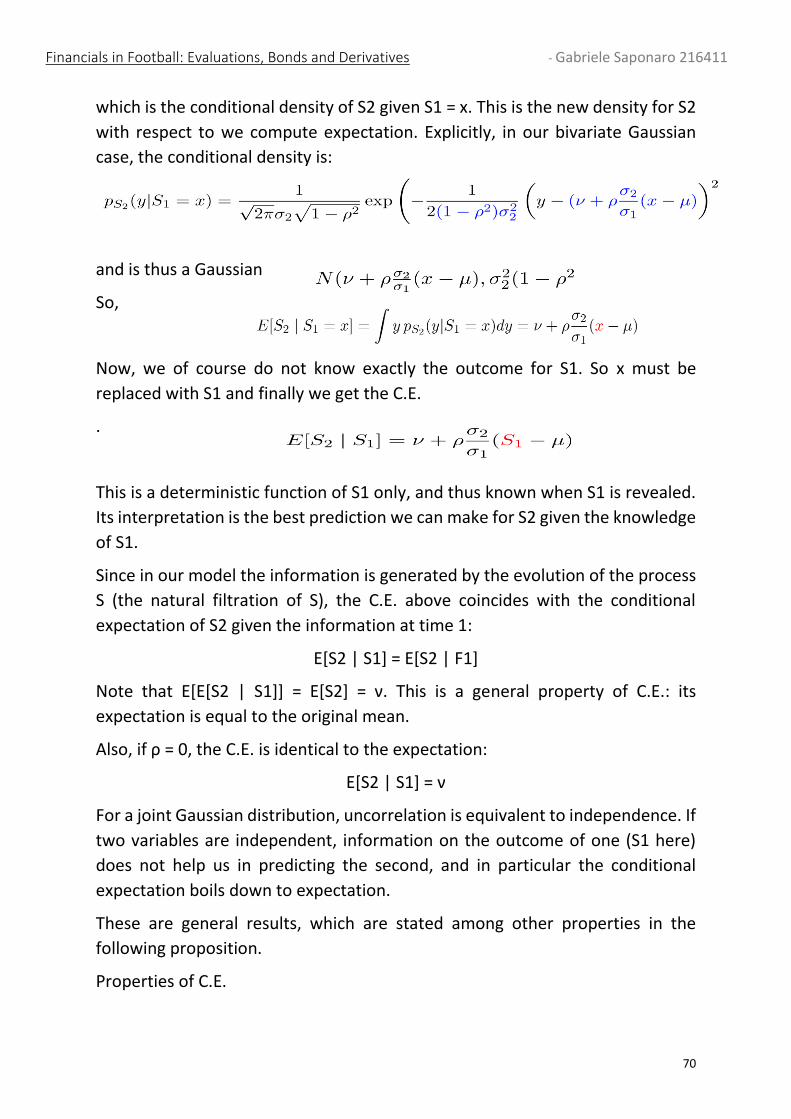
Financials in Football: Evaluations, Bonds and Derivatives - Gabriele Saponaro 216411
70
which is the conditional density of S2 given S1 = x. This is the new density for S2
with respect to we compute expectation. Explicitly, in our bivariate Gaussian
case, the conditional density is:
and is thus a Gaussian
So,
Now, we of course do not know exactly the outcome for S1. So x must be
replaced with S1 and finally we get the C.E.
.
This is a deterministic function of S1 only, and thus known when S1 is revealed.
Its interpretation is the best prediction we can make for S2 given the knowledge
of S1.
Since in our model the information is generated by the evolution of the process
S (the natural filtration of S), the C.E. above coincides with the conditional
expectation of S2 given the information at time 1:
E[S2 | S1] = E[S2 | F1]
Note that E[E[S2 | S1]] = E[S2] = ν. This is a general property of C.E.: its
expectation is equal to the original mean.
Also, if ρ = 0, the C.E. is identical to the expectation:
E[S2 | S1] = ν
For a joint Gaussian distribution, uncorrelation is equivalent to independence. If
two variables are independent, information on the outcome of one (S1 here)
does not help us in predicting the second, and in particular the conditional
expectation boils down to expectation.
These are general results, which are stated among other properties in the
following proposition.
Properties of C.E.

Financials in Football: Evaluations, Bonds and Derivatives - Gabriele Saponaro 216411
71
E[E[Y | X]] = E[Y ]
additivity: E[Y1 + Y2 | X] = E[Y1 | X] + E[Y2 | X]
Let f be a deterministic function; then,
E[f(X)Y | X] = f(X)E[Y | X]
that is, random variables which are known when X is known can be treated like
constants and taken out of the conditional expectation sign. In particular, by
taking Y = 1,
E[f(X) | X] = f(X)
If two variables (X,Y ) are independent then the conditional expectation of one
with respect to the other is constant, and coincides with the mean
E[Y | X] = E[Y ];E[X | Y ] = E[X]
Conditional expectation E[Y |X], similarly to its relative the expectation, is a
notion which heavily depends upon P. If we changed our probabilistic views, the
resulting average of outcomes would change: we would get a different random
variable.
Conditional expectation with respect to information and martingales Let us go
back to our filtered space (Ω,(Ft)t≤T ,P).
It is the best prediction of the random variable Y given the information we (will)
possess in t1. As for the conditional expectation with respect to random
variables, this conditional expectation is an average of the outcomes of Y given
the knowledge we are supposed to have in t1. So, E[Y | Ft1] is a random variable,
known in t1.
So given a filtered space, fix 0 ≤ t0 < t1 < t2 ≤ T, and let Y,W be random variables
(know at least in T).
E[E[Y | Ft1]] = E[Y ];
if Y is known by time t1, then \E[Y | Ft1] = Y ;
additivity: E[Y + W | Ft1] = E[Y | Ft1] + E[W | Ft1]
for any Z known by time t1,
E[ZY | Ft1] = ZE[Y | Ft1]
If Y is independent of Ft1, then
E[Y | Ft1] = const = E[Y ]
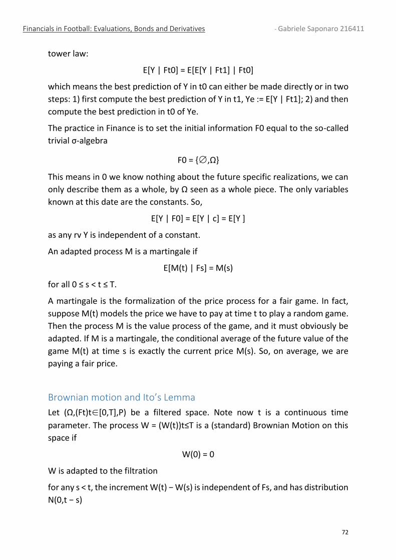
Financials in Football: Evaluations, Bonds and Derivatives - Gabriele Saponaro 216411
72
tower law:
E[Y | Ft0] = E[E[Y | Ft1] | Ft0]
which means the best prediction of Y in t0 can either be made directly or in two
steps: 1) first compute the best prediction of Y in t1, Ye := E[Y | Ft1]; 2) and then
compute the best prediction in t0 of Ye.
The practice in Finance is to set the initial information F0 equal to the so-called
trivial σ-algebra
F0 = ∅,Ω
This means in 0 we know nothing about the future specific realizations, we can
only describe them as a whole, by Ω seen as a whole piece. The only variables
known at this date are the constants. So,
E[Y | F0] = E[Y | c] = E[Y ]
as any rv Y is independent of a constant.
An adapted process M is a martingale if
E[M(t) | Fs] = M(s)
for all 0 ≤ s < t ≤ T.
A martingale is the formalization of the price process for a fair game. In fact,
suppose M(t) models the price we have to pay at time t to play a random game.
Then the process M is the value process of the game, and it must obviously be
adapted. If M is a martingale, the conditional average of the future value of the
game M(t) at time s is exactly the current price M(s). So, on average, we are
paying a fair price.
Brownian motion and Ito’s Lemma
Let (Ω,(Ft)t∈[0,T],P) be a filtered space. Note now t is a continuous time
parameter. The process W = (W(t))t≤T is a (standard) Brownian Motion on this
space if
W(0) = 0
W is adapted to the filtration
for any s < t, the increment W(t) − W(s) is independent of Fs, and has distribution
N(0,t − s)

Financials in Football: Evaluations, Bonds and Derivatives - Gabriele Saponaro 216411
73
the paths W(·,ω) are continuous
Marginal distributions are Gaussian. For any t, W(t) can be written as W(t) −
W(0), so from 3) above it has distribution N(0,t).
Independent, identically distributed increments (BM is a process with IID
increments). Since W(u), for any u ≤ s is known at time s, as the Brownian Motion
is adapted, from property 3) above it follows that for any u ≤ s < t the variables
W(u),W(t) − W(s)
are independent, and therefore jointly Gaussian . This
argument can be extended to any number of increments, i.e. if 0 ≤ t1 < ...tn ≤ T
then
W(t1),W(t2) − W(t1),...W(tn) − W(tn−1)
are independent and thus jointly Gaussian with distribution
This shows the distribution of any family of increments depends only on the time
distance at which the increments are sampled (identically distributed
increments).
Brownian Motion W is a martingale.
Proof. Fix two arbitrary dates s < t and write W(t) = W(t) − W(s) + W(s). Then,
E[W(t) | Fs] = E[W(t) − W(s) + W(s) | Fs] = W(s) + E[W(t) − W(s)] = W(s)
given the properties of the conditional expectation.
A Brownian motion with drift b and volatility σ > 0 is the process
B(t) = bt + σW(t)
which is a linear transform of the (standard) Brownian motion W.
The processes L which, like the BM, have IID increments and satisfy
P(L(t) = L(t−)) = 1 for all t ∈ (0,T]
are called L´evy processes. These generalizations of BM may admit jumps, but
only at stochastic, ‘unpredictable’ times.
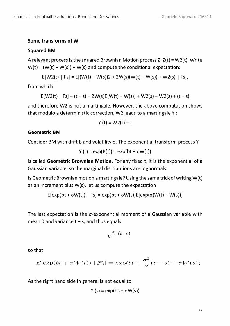
Financials in Football: Evaluations, Bonds and Derivatives - Gabriele Saponaro 216411
74
Some transforms of W
Squared BM
A relevant process is the squared Brownian Motion process Z: Z(t) = W2(t). Write
W(t) = (W(t) − W(s)) + W(s) and compute the conditional expectation:
E[W2(t) | Fs] = E[(W(t) − W(s))2 + 2W(s)(W(t) − W(s)) + W2(s) | Fs],
from which
E[W2(t) | Fs] = (t − s) + 2W(s)E[W(t) − W(s)] + W2(s) = W2(s) + (t − s)
and therefore W2 is not a martingale. However, the above computation shows
that modulo a deterministic correction, W2 leads to a martingale Y :
Y (t) = W2(t) − t
Geometric BM
Consider BM with drift b and volatility σ. The exponential transform process Y
Y (t) = exp(B(t)) = exp(bt + σW(t))
is called Geometric Brownian Motion. For any fixed t, it is the exponential of a
Gaussian variable, so the marginal distributions are lognormals.
Is Geometric Brownian motion a martingale? Using the same trick of writing W(t)
as an increment plus W(s), let us compute the expectation
E[exp(bt + σW(t)) | Fs] = exp(bt + σW(s))E[exp(σ(W(t) − W(s))]
The last expectation is the σ-exponential moment of a Gaussian variable with
mean 0 and variance t − s, and thus equals
so that
As the right hand side in general is not equal to
Y (s) = exp(bs + σW(s))
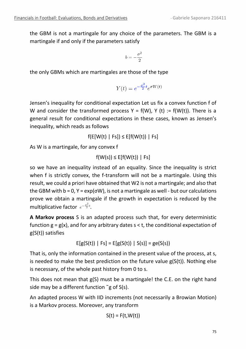
Financials in Football: Evaluations, Bonds and Derivatives - Gabriele Saponaro 216411
75
the GBM is not a martingale for any choice of the parameters. The GBM is a
martingale if and only if the parameters satisfy
the only GBMs which are martingales are those of the type
Jensen’s inequality for conditional expectation Let us fix a convex function f of
W and consider the transformed process Y = f(W), Y (t) := f(W(t)). There is a
general result for conditional expectations in these cases, known as Jensen’s
inequality, which reads as follows
f(E[W(t) | Fs]) ≤ E[f(W(t)) | Fs]
As W is a martingale, for any convex f
f(W(s)) ≤ E[f(W(t)) | Fs]
so we have an inequality instead of an equality. Since the inequality is strict
when f is strictly convex, the f-transform will not be a martingale. Using this
result, we could a priori have obtained that W2 is not a martingale; and also that
the GBM with b = 0, Y = exp(σW), is not a martingale as well - but our calculations
prove we obtain a martingale if the growth in expectation is reduced by the
multiplicative factor .
A Markov process S is an adapted process such that, for every deterministic
function g = g(x), and for any arbitrary dates s < t, the conditional expectation of
g(S(t)) satisfies
E[g(S(t)) | Fs] = E[g(S(t)) | S(s)] = ge(S(s))
That is, only the information contained in the present value of the process, at s,
is needed to make the best prediction on the future value g(S(t)). Nothing else
is necessary, of the whole past history from 0 to s.
This does not mean that g(S) must be a martingale! the C.E. on the right hand
side may be a different function ˜g of S(s).
An adapted process W with IID increments (not necessarily a Browian Motion)
is a Markov process. Moreover, any transform
S(t) = F(t,W(t))
Financials in Football: Evaluations, Bonds and Derivatives - Gabriele Saponaro 216411
76
via a deterministic function F(t,x) which is invertible wrt the x variable for every
fixed t is also a Markov process.
Fix s < t and consider any deterministic g = g(x). Then,
g(W(t)) = g((W(t) − W(s)) + W(s))
The increment Z = W(t) − W(s) is independent of Fs and the only other variable
showing up is W(s). Then
E[g(W(t)) | Fs] = E[E[g(W(t)) | W(s)]] = g(z + W(s))pt−s(z)dz
in which pt−s indicates the density of the increment. Note also that the function
ge can be read in the above formula: ge(x) = g(z + x)pt−s(z)dz
For demonstration, fix a deterministic function g and consider g(S). Fix t > s and
consider
g(S(t)) = g(F(t,W(t)) = h(W(t))
where we set h(x) = g(F(t,x)) and therefore the C.E. of g(S(t)) is
E[g(S(t)) | Fs] = E[h(W(t)) | Fs] = eh(W(s))
W(s) can be written in terms of S(s) since F(s,·) is invertible in x! If this inverse is
denoted by F−1(s,x), finally
E[g(S(t)) | Fs] = ge(S(s))
where ge(x) := eh(F−1(s,x)).
This is the reason why deterministic functions F(t,x) are called ‘Markovian’: then
(F(t,W(t))t is a Markov process.
The BM with drift and the GMB are Markov processes.
Ito’s formula
Ito’s formula gives the dynamics of any smooth Markovian function of the BM
W.
Knowing the dynamics (=the infinitesimal variations of the process) is quite
useful, especially for simulation purposes.
Consider a deterministic, smooth function F of two variables (t,x). Then, F varies
only in response to changes in (t,x), according to the following equation
dF(t,x) = Ft(t,x)dt + Fx(t,x)dx

Financials in Football: Evaluations, Bonds and Derivatives - Gabriele Saponaro 216411
77
which represents the infinitesimal change in the value of F,
dF(t,x) := F(t+dt,x+dx)−F(t,x)
when we move from (t,x) to (t+dt,x+dx) as a sum of the infinitesimal changes in
the variables amplified by the proper partial derivatives.
A second order approximation would be
but as the terms between parentheses are negligible wrt the others, we never
see them explicitly when writing infinitesimal variations.
Interpret t as a time parameter, and consider the stochastic process
Y (t) = F(t,W(t))
in which W is a standard BM. The variation of Y can be described in terms of the
variations of time and W using :
The reason why we go to the second order is that the paths of W are very wild.
They are continuous, yes, but non-differentiable, so we are not sure about the
order of the last group of terms between parentheses. In fact, it turns out that:
(dW(t))2 ∼ dt
while of course (dt)2 and the product dW(t)dt are of higher order than dt.
The intuition is that
dW(t) = W(t + dt) − W(t) ∼ N(0,dt)
and so we approximate the squared increment with its mean dt.
Ito’s Lemma
Let F(t,x) be a smooth function (the minimal regularity required is C1,2(t,x)). The
Markov process defined by
F(t,W(t))
has dynamics given by the (stochastic) differential equation

Financials in Football: Evaluations, Bonds and Derivatives - Gabriele Saponaro 216411
78
Note the difference with ordinary calculus: the blue, extra term above is known
as It¯o’s term.
Diffusion processes
An It¯o process is any adapted process Y whose dynamics may be written as
dY (t) = α(t)dt + β(t)dW(t)
where α and β are adapted processes which are called the coefficients of the
stochastic differential equation. The first coefficient, α, is called the drift -
though in Finance, when Y is a positive price process, only the fraction is
called ‘the drift’. The second coefficient, β, is the diffusion coefficient.
Thanks to the It¯o’s formula, any Markovian function Y (t) = F(t,W(t)) of W is a
diffusion.
In the BM and GBM cases, we have shown that these processes are martingales
if and only if the drift is 0. For a general diffusion, we state the following result.
If a diffusion Y is a martingale, necessarily the drift vanishes. Conversely, if the
drift vanishes and the diffusion coefficient satisfies an integrability condition:
then the diffusion is a martingale.
Therefore, the only diffusions candidates to the martingale property are those
of the form
dY (t) = β(t)dW(t)
and these are true martingales if β is good. Without extra conditions on β a
diffusion with zero drift is only a local martingale.
An intuitive idea of why the drift must vanish when the diffusion is a martingale
is the following. By definition, any martingale M has conditional increments ∆M
= M(t + ∆t) − M(t) with zero C.E. :
E[M(t + ∆t) − M(t) | Ft] = 0
If the time difference becomes infinitesimal, then E[dM(t) | Ft] = 0 for any t. For
a general diffusion Y we have
E[Y (t + dt) − Y (t) | Ft] = E[dY (t) | Ft] = α(t)dt + β(t)E[dW(t) | Ft] = α(t)dt
Financials in Football: Evaluations, Bonds and Derivatives - Gabriele Saponaro 216411
79
since α and β are adapted, thus known at time t, and dW(t) is an infinitesimal
centered Gaussian increment, independent of Ft. If Y is a martingale, then
E[dY (t) | Ft] = 0 = α(t)dt
for all t, which means α = 0.
The converse is more complicated. In fact, if α = 0 then we must control how the
infinitesimals add up, in order to be sure that the resulting process is a
martingale. This is the reason why an integrability condition on β is needed to
ensure the martingale property in Proposition
It¯o’s formula for diffusions Suppose a diffusion S is assigned:
dS(t) = α(t)dt + β(t)dW(t)
and consider a deterministic, Markovian transform of the diffusion S
P(t,S(t))
If S models a stochastic price process of a stock, then the price process of any
European call option is exactly a Markovian transform of S.
Therefore, we are interested in the dynamics of P and we wonder if there is a
formula: the answer is positive. Exactly as we have seen in the Markovian
transforms of the standard BM W, there is an It¯o’s formula for the Markovian
transforms of any diffusion S:
Since (dS(t))2 ∼ β(t)2dt, we can equivalently write
The Black-Scholes’ world The famous Black-Scholes(-Merton) 1973 formula for option prices is a
milestone in Finance. It can be found everywhere, from Wikipedia and
practitioners’ booklets to the Financial press and all graduate texts on
Mathematical Finance.
The pricing of derivatives is a relative pricing: derivatives are priced in terms of
the assigned price dynamics of the basic financial instruments.
Financials in Football: Evaluations, Bonds and Derivatives - Gabriele Saponaro 216411
80
The basic financial instruments in the Black-Scholes model are only two. This is
the minimal number of basic assets to have in order to be able to construct
portfolios (mixed investments). The first instrument is the money market
account (B, the ‘bond’) and the second is the ‘stock’ S. The bond is assumed to
be riskless, and continuously paying a constant interest rate r ≥ 0:
dB(t) = rB(t)dt B(0) = 1
or B(t) = ert. B should be regarded as a capitalization factor.
The other basic instrument is the risky stock, which is required to satisfy the SDE
+ initial condition (Cauchy problem)
dS(t) = µS(t)dt + σS(t)dW(t)
S(0) = S0
where S0 is the observed initial market price, and µ, σ are constants (σ > 0).
These latter parameters are called drift and volatility respectively. From the
general theory on SDEs, the above Cauchy problem has a unique solution, and
since we already know a solution, S must be:
In particular, the marginals S(t) satisfy
That is, mean and variance of the stock logreturn grow linearly with time.
E[S(t)] = S0eµt,
We realize µ is the exponential growth of the average stock price. We may then
be concerned with arbitrage possibilities. What if µ ≥ r, or µ < r? In the first case,
one may be tempted to borrow money from the bank, and invest everything in
stock; in the other case, one may think of selling short the stock, and invest in
the bond. However, neither of these strategies leads to an arbitrage. In fact,
while B deterministically increases at rate r, the stock increases at rate µ only in
average (in expectation). So, depending on the particular path, and as a
consequence of the noise effect, for any t the marginal S(t) (which is a
lognormal) can be below S0ert even if µ > r; and it can be above S0ert even if µ
< r.

Financials in Football: Evaluations, Bonds and Derivatives - Gabriele Saponaro 216411
81
We end by noting that µ and σ have also an ‘instantaneous’ meaning. The ratio
is the return of the stock on the infinitesimal interval (t,t + dt) and thus: µ is
the conditional rate of return of the stock
and σ2 is the conditional rate of variance:
Portfolio strategies
A portfolio in stock and bond is the most intuitive concept of all. In order to
develop rigorous Maths, we are going to formalize it a bit.
A portfolio strategy, or simply a strategy, is a couple of adapted processes (K,H)
where H(t) is the number of stock shares held at t and K(t) is the number of bond
shares. Therefore, at any instant t the portfolio value V is given by
V (t) = K(t)B(t) + H(t)S(t)
The simplest example is a buy-and-hold strategy, consisting of a couple of
constant processes (K0,H0). In practice, we choose at time 0 the positions in
stock and bond and keep them till T.
The initial cost of this strategy is V (0) = K0 +H0S0 and the value process of the
corresponding portfolio is:
V (t) = K0ert + H0S(t)
Of course, buy-and-hold strategies form a very small set in a continuous time
market: active trading occurs only at 0 and at the final date T, when the positions
are closed. Suppose now that trading occurs along a pre-specified finite time
grid
t0 = 0 < t1 < ... < tn = T
Now, a strategy is piecewise-constant and can be identified with K(ti),H(ti) for i
= 0...n − 1 , where for each i K(ti),H(ti) are the positions in bond and stock to be
held from time ti up to time ti+1:
K(t) = K(ti),H(t) = H(ti) if t ∈ [ti,ti+1)
For times t before t1, 0 ≤ t < t1, the value V clearly is
Financials in Football: Evaluations, Bonds and Derivatives - Gabriele Saponaro 216411
82
V (t) = K(t0)B(t) + H(t0)S(t) = K0B(t) + H0S(t)
At the initial time, to implement the strategy we must start with initial wealth
w0 equal to V (0) = K0 + H0S0. We arrive in t1 with wealth
since the processes B,S are continuous. To implement the strategy in the second
step we should possess the wealth
w2 = V (t1) = K(t1)B(t1) + H(t1)S(t1)
This other wealth can be obtained by external infusion of money in case w1 <
w2, or by consumption if the opposite inequality holds. If w1 = w2, at the date
t1 and at all the subsequent trading dates, the portfolio strategy is called self-
financing. With continuous processes, the self-financing condition on a finite
grid amounts to the continuity of V globally on [0,T], trading dates included.
A self-financing strategy is thus obtained by starting with an initial endowment
w0, and then (re-)allocating money between stock and bond at the trading dates
with no infusion and no withdrawal of money.
The self-financing equations, which must hold at any trading date ti,i > 0 are
K(ti−1)B(ti) + H(ti−1)S(ti) = K(ti)B(ti) + H(ti)S(ti)
dV (t) = K(ti)dB(t) + H(ti)dS(t)
dV (t) = K(t)dB(t) + H(t)dS(t)
This means that the variations in value of a self-financing portfolio are
proportional to the changes in value of bond and stock, the coefficients being
the number of shares held.
This is the limit obtained when portfolio re-adjustments are infinitesimally close
to each other.
A general portfolio strategy (H,K) is called self-financing if the above equation
holds on [0,T]. In particular, any self-financing portfolio is a diffusion.
For a self-financing portfolio it is equivalent to know:
the couple (H,K), V (0) and one of H, K.
The choice is usually to give V (0) (the initial wealth) and H, the position in the
risky stock.
Financials in Football: Evaluations, Bonds and Derivatives - Gabriele Saponaro 216411
83
The reason is the following. If we work with discounted quantities, i.e. with the
processes
then this latter verifies dVe = HdSe.
Therefore, if one knows V (0) = Ve(0) and H, thanks to the above SDE also Ve is
known and K can then be computed using the relation
K(t)B(t) + H(t)S(t) = V (t) = ertVe(t)
Arbitrage and martingale measures: the First Fundamental Theorem of Asset
Pricing
Finite trading dates market
An arbitrage strategy in a finite time market model is a self-financing strategy V
(0),H such that
V (0) = 0
V (T) ≥ 0 and P(V (T) > 0) > 0
Thus an arbitrage is a strategy which makes money out of nothing: it starts with
zero money, and in a self-financing way leads to a non-negative wealth, which is
positive with positive probability. So, if such strategies existed, one would get a
positive gain with positive probability at no cost and without risk.
If an arbitrage opportunity were present in a real market, all the (smart)
investors would try to take advantage of it simultaneously. Therefore, prices of
the underlying financial instruments would not be at equilibrium, as there would
be an almost instantaneous move of the prices as a response to a supply-
demand imbalance. This price movement would continue until any opportunity
for riskless profit is no longer available.
This is the rationale behind the construction of models were No Arbitrage
(mathematically defined above, NA for short in the sequel) strategy is present.
In the Cox-Ross-Rubinstein (binomial tree) model, with capitalization factor m =
er and stock multipliers eu,ed, the NA condition holds if an only if
d < r < u
and this is exactly the condition one puts on the parameters in order to develop
option pricing.
Financials in Football: Evaluations, Bonds and Derivatives - Gabriele Saponaro 216411
84
Dalang-Morton-Willinger
Given a finite time filtered probability space (Ω,(Fti)i=0...n,P) and a market
model (B,S), where S is the (possibly multidimensional) risky asset and B is the
bond, NA is equivalent to the existence of a probability Q on FT with the
properties:
Q(A) = 0 if and only if P(A) = 0 [Q is equivalent to P, notation Q ∼ P]
the discounted stock price process is a Q-martingale, i.e.
Such Q, which is not necessarily unique, is called an equivalent martingale
measure (EMM) for Se.
The second property above better reads as current prices for S are expected
values of discounted future values under Q:
which when s = 0 reads
S(0) = EQ[e−rtS(t)]
This fundamental relation has the financial meaning that Q calibrates S.
The FTAP is the basis of the use of martingale methods in Finance. The
philosophy behind it goes as follows.
Suppose the model bond-stock (B,S) verifies the NA condition. Then, by the FTAP
implication: NA ⇒ existence of an EMM, there exists (at least) one EMM Q.
Suppose we would like to launch a derivative on S, with payoff Ψ and maturity
T (with no early exercise feature). We would like to place the derivative on the
market with a fair price P. By fair price we mean that the extended market
(B,(S,P)) must also verify NA, in the sense that there exists no arbitrage strategy
(K,H,J) based on stock-bond-derivative, and this latter with price P. Obviously, at
the maturity T P(T) = Ψ. What about indermediate dates? The solution is to set
Financials in Football: Evaluations, Bonds and Derivatives - Gabriele Saponaro 216411
85
or, equivalently, dividing by B(t)
If the price P verifies the above condition, the probability Q, which is an EMM
for Se, is an EMM also for the discounted Pe thanks to its definition above and
to the terminal condition P(T) = Ψ.
So, Q is an EMM for the bidimensional risky process (S,P). Therefore, the FTAP,
converse implication, existence of an EMM ⇒ NA, implies the extended market
verifies NA.
In particular, a fair initial price is
P(0) = EQ[e−rT Ψ]
that is prices must be computed as Q-expectations of discounted payoffs.
As a final remark, remember that Q may be very different from P and it should
be regarded only as a pricing tool.
Portfolio selection (optimization) and, more generally, any risk management
issue must all be addressed under P, that is
compute P(S(T) > K)
compute E[U(V (T))] if U is the agent’s utility function, and E is P-expectation
consider the supremum over a class V of portfolios of some performance
criterion, e.g. expected utility maximization supV ∈V E[U(V (T))] or Markowitz’s
mean-variance optimization.
General markets
The FTAP in the version we presented holds for markets open only on a finite
number of dates (like the Cox-Ross-Rubinstein model).
In general, for market models open on infinite trading dates (discrete but infinite
dates, like in asymptotic problems, or continuous time as Black-Scholes) we
must add a condition to the arbitrage portfolios.
An arbitrage strategy is a self-financing strategy V (0),H such that
V (0) = 0
Financials in Football: Evaluations, Bonds and Derivatives - Gabriele Saponaro 216411
86
there exists a constant c > 0 such that V (t) ≥ −c for all t ∈ (0,T) c here is a finite
credit line which must be respected during the trading, and it may depend on H
V (T) ≥ 0 and P(V (T) > 0) > 0
The market verifies No Arbitrage (NA) if no such strategy exists.
For generale markets, to get a consistent pricing rule one needs to exclude not
only arbitrage strategies, but also certain limits of self-financing strategies,
which are ‘asymptotic arbitrages’ and are called Free Lunches with Vanishing
Risk (FLVR).
So, if we can exhibit an EMM Q for Se, then the same reasoning we made above
for the pricing of a new derivative applies.
Pricing principle Suppose Q is an EMM for S and consider a European option
payoff Ψ, with maturity T. Then, if
P(t) = EQ[e−r(T−t)Ψ | Ft]
the extended model (B,S,P) verifies NFLVR and also the weaker condition NA.
This approach seems quite abstract, but it is powerful as it is very general. In
fact, it applies to any market model (not only to Black-Scholes) and to all types
of payoffs with no early exercise features, including path-dependent ones like
Asian options:
or
like lookbacks:
Ψ1 = S(T) − minS(t) or Ψ2 = maxS(t) − S(T) t≤T t≤T
and barrier options. We will see this is not the case for the PDE based methods,
which work only for Markovian derivatives of the type g(S(T)), functions of S at
the maturity date only.
Pricing and hedging are closely related: the Second FTAP
There is evidently a link between pricing and hedging. Suppose a derivative Ψ
with maturity T can be replicated/perfectly hedged, there exists a self-financing
portfolio V in stock and bond such that
V (T) = Ψ
Financials in Football: Evaluations, Bonds and Derivatives - Gabriele Saponaro 216411
87
then there is only one way of pricing the derivative without introducing arbitrage
in the extended market (stock, bond, derivative):
P(t) = V (t)
In some sense, the replicable derivatives are redundant: they can be
synthetically reproduced using stock and bond. The number of stock shares used
in the replication, H, in jargon is often called the Delta (∆) of the derivative.
Of course, the martingale method and the hedging-based method must give the
same result. This is due to the fact that any self-financing portfolio verifies
dVe = HdSe
and if H is good enough then Ve is a martingale when Se is. So, under any EMM
Q we have:
and therefore
coincides with V (t).
An easy example of replicable contract is a forward contract. The strategy is of
buy-and-hold-type, with H(t) = H0 ≡ 1.
The market is complete if all the derivatives are replicable.
So, if a market is complete, any fixed derivative has only one fair price,
corresponding to the value of the replicating portfolio.
Any real market is incomplete: one cannot perfectly hedge out all conceivable
risk. Nevertheless, in this course we consider only two models, and both are
complete: the Cox-Ross-Rubinstein model, and the Black-Scholes one. For
arbitrage free market models, the Second FTAP characterizes completeness.
Consider a market model verifying NFLVR. Then, the following are equivalent
the market is complete there exists only one Q EMM for Se.
Financials in Football: Evaluations, Bonds and Derivatives - Gabriele Saponaro 216411
88
Valuation of options in Black-Scholes Let us go back to the Black-Scholes model, and let us exhibit a Q which is the
unique EMM for Se, the discounted stock price. Since
dS = µSdt + σSdW,
then has dynamics given by
So, Se is not a martingale under P in general.
The market price of risk financially represents the instantaneous excess return
over the riskless rate µ − r per unit of volatility, and should remind the reader of
the Sharpe Ratio. Set
W∗(t) = W(t) + λt
and note
dW∗ = dW + λdt
Written in terms of W∗, the SDE for Se reads as
dSe = σSdWe ∗
If there existed a probability Q ∼ P such that W∗ were a Q-Brownian motion,
we would immediately conclude Q is a martingale probability for Se. And this is
in fact the case.
An important probabilistic result, called Girsanov Theorem, ensures that there
exists a unique Q with this property, and gives the explicit transform which links
Q to P. So, by the second FTAP, we also know that the market is complete: any
derivative with no early-exercise feature is replicable. The transform provided
by the Girsanov theorem is the Radon-Nikodym density of Q wrt P, which is a
random variable equal to
Financials in Football: Evaluations, Bonds and Derivatives - Gabriele Saponaro 216411
89
The strict positivity of such function ensures that Q is equivalent to P. The
knowledge of the density function in fact allows to compute the Q probabilities
in terms of deformed P probabilities
as the indicator IA is weighted by the ’deformation’ density function prior to
taking Pexpectation. Anyway, the best thing to do when computing prices here
is to think only about the effect of the change of measure on Se, which becomes
martingale GBM under Q, i.e.
Se(t) = exp(−σ2t/2 + σW∗(t))
which is equivalent to say that S is
S(t) = Se(t)ert = S0 exp((r − σ2/2)t + σW∗(t))
or also
dS = rSdt + σSdW∗
The drift of S under Q is r. So, on average, under Q the stock is a GBM with the
same σ, but grows at the rate of the riskless bond. This is the reason why Q is
called a risk neutral measure. Even if the investor is risk averse, when pricing she
behaves as if she were risk neutral.
If the derivative has maturity T and is of the simple Markovian form g(S(T)), then
its price today is
whence we are left with the computation of the one dimensional integral
which may be impossible to compute analytically. In any case, it can be
approximated via simulation. If we wish to know the price at time 0 < t < T, then
P(t) = EQ[e−r(T−t)g(S(T)) | Ft]
This also leads to the computation of an integral. The idea is to write
S(T) = S(t)exp((r − σ2/2)(T − t) + σ(W∗(T) − W∗(t))),
Financials in Football: Evaluations, Bonds and Derivatives - Gabriele Saponaro 216411
90
so that the only dependence of g(S(T)) from the past up to t is contained in the
term S(t), while the factor exp((r − σ2/2)(T − t) + σ(W∗(T) − W∗(t))) is
independent of Ft. So,
where τ = T − t is the time to maturity . The formula looks the same, only S0 must
be replaced by S(t) (random, but known at t) and T by τ. If we call G the
deterministic function
then we realize the price process is a Markovian function of S:
G(t,S(t))
If the payoff is more complicated, like in a path dependent case, often the only
way is resorting to simulation.
The payoff is of the form for Asian options.
Note that the conditional expectation of the discounted payoff say at any t4 > t
> t3 depends not only on S(t), but also on S(t1),S(t2),S(t3).
Suppose for simplicity the average of the stock is made only on two dates, t1
and t2 = T.
Since , simulate
two independent standard Gaussian variables Z,Y and call z1,y1 the outcomes.
Set
and compute the max m1 between v1 −K and 0. Repeat the algorithm sufficiently
many times’ and average the values. This average, discounted, is the
approximate value of the option:
Financials in Football: Evaluations, Bonds and Derivatives - Gabriele Saponaro 216411
91
Stochastic discount factor In many books for economists, pricing is made by
referring to the ’stochastic discount factor’ (SDF) and then taking P-
expectations. The price of any derivative with payoff Ψ is given by
P(t) = EQ[e−r(T−t)Ψ | Ft]
and ).
Q-conditional expectation via P. Note first that if L denotes the process
then L is a P-martingale with terminal value and with L(0) = 1. Thanks
to the abstract version of Bayes’ Theorem for conditional expectation, we can
write:
in which the second equality follows from the martingale property of L. So, if
D(t;T) denotes the variable
D(t) = e−rtL(t)
then the process M with M(t) := P(t)D(t) is a P martingale with terminal value
ΨD(T) (the martingale property follows from the tower law of conditional
expectation) and the price at any t can be computed as
and at time 0, P(0) = E[D(T)Ψ]. This is why the process D is called the SDF: it
incorporates both the discounting and the change of probabilistic views. The
moral is: we can compute prices as P expectations, if we first let the SDF act as
a multiplicative deformation on the payoff Ψ.
The formula for the price of a call option
The final formula for the price C(0) of a call with maturity T and strike K is
C(0) = S0Φ(d1) − Ke−rT Φ(d2)
where Φ is the standard Gaussian CDF,
Financials in Football: Evaluations, Bonds and Derivatives - Gabriele Saponaro 216411
92
and, at any intermediate t,
C(t,S(t)) = S(t)Φ(d1(t)) − Ke−rτΦ(d2(t))
where τ = T − t and di(t),i = 1,2 are
Note the ’historical’ drift µ has vanished from the valuation formula, as
expected.
The price of the corresponding put option can be found either by direct
calculations, similar to the ones seen for the call, or more easily via the put-call
parity.
The valuation PDE in Black-Scholes and the Delta
The derivation method of the Black-Scholes valuations PDE is very important, as
it gives as a byproduct the structure of the replicating portfolio for any given
Markovian payoff g(S(T)). The scheme is the following:
Fix a payoff g(S(T)); its unique price at time t will be a Markovian function of time
and S(t) only: let us call it
G(t,S(t))
Apply It¯o’s formula to G
Identify the self-financing strategy (K,H) which replicates g(S(T))
Derive a valuation PDE with terminal condition solve the PDE, and get the Delta
of an option Let us go through the steps.
This point is heuristically assumed in the original article by Black and Scholes,
but we already know it is correct on the martingale method.
It¯o’s formula gives:
that is
Financials in Football: Evaluations, Bonds and Derivatives - Gabriele Saponaro 216411
93
If the derivative admits a replicating portfolio, necessarily its value V (t) = H(t)S(t)
+ K(t)B(t) must coincide with G, so that dG(t,S(t)) = dV (t) = K(t)dB(t) + H(t)dS(t)
= K(t)rertdt + H(t)dS(t) therefore, we get two equations, one for H and one for
K: 1) H(t) = Gs(t,S(t)) and 2)
.
As Kert = K(t)B(t) = V (t) − H(t)S(t) = G(t,S(t)) − H(t)S(t) then
This equation must be satisfied for every 0 ≤ t < T. Since when t is fixed S(t) is a
lognormal, which can assume any positive real value, we can replace the random
S(t) with the positive real parameter s and write the famous, parabolic valuation
PDE:
which is the same for all the derivatives. It is a linear, parabolic PDE where only
the interest rate and volatility enter, while µ has vanished.
The specific derivative enters only in the terminal condition, so we face a Cauchy
problem:
with the terminal condition G(T,s) = g(s). Such Cauchy problem has a unique
solution.
Since the Cauchy problem has a unique solution, we also prove that any
Markovian derivative can be replicated in a self financing way using stock and
bond. In fact, if we can solve the above Cauchy problem, and explicitly find G,
then we can immediately find H (and K by difference), thanks to the self-
financing condition:
The number of shares of the risky stock which are necessary for the replication
(a.k.a. the Delta of the option) is simply the derivative of the function G with
respect to the stock s, composed with the current level of the stock S(t):
H(t) = Gs(t,S(t))
It is the sensitivity of the option price wrt stock movements.
Financials in Football: Evaluations, Bonds and Derivatives - Gabriele Saponaro 216411
94
How to solve the Cauchy problem? there are three possible solutions:
1) analytical methods, by reducing the valuation PDE to the heat equation;
2) numerical methods (discretization of the PDE via numerical schemes like
finite differences, etc)
3) the Feynman-Kaˇc probabilistic representation, which gives the same
representation obtained by the martingale method.
The Delta for a call option at time t is Φ(d1(t)). The easiest way to show it directly
from the formula for the option price (4), substituting S(t) = s and taking the s
derivative of C. Note this is a positive number, smaller than 1 .
For a put, the situation is quite different: its Delta is negative, and equals
−Φ(−d1). This can be derived either by differentiation of the put price, or using
the put call parity:
P(t,s) = C(t,s) − s + Ker(T−t)
and differentiating wrt s the right hand side.
An example of Delta hedging can be a trader sells a call option at a price c∗,
which may differ from the Black Scholes price C0. The trader has now an (extra)
exposition −Φ(d1) to the stock movements (this is the Delta of a short call). To
neutralize the effects of stock movements, she invests in stock and bond so to
keep the global portfolio: call, positions in stock and bond Delta neutral. So, she
starts following the replicating portfolio V in stock and bond for the call. This
portfolio exactly prescribes to buy Φ(d1) shares of S. So, globally the Delta will
be zero.
The initial cost of the replicating strategy is the Black-Scholes price of the call C0.
By adjusting the Delta continuously, i.e. continuously buying and selling shares
in order to possess Φ(d1(t)) at any time t, she will finally end up at T with:
V (T) − (S(T) − K)+ + (c∗− C0)erT = (c∗ − C0)erT
So, whatever is c∗, the final payoff is non-random: the risk has been eliminated.
As long as a portfolio is self-financed and Delta neutral, there are no other risks.
And if c∗ > C0 the trader has even made a positive gain - so, we have described
an arbitrage! This is a faithful picture of what happens in practice. ‘Fair’ prices
are computed on a hedging basis, and then an ‘add-on’ is charged by the
trader/financial institution (here, the difference c∗ − C0). Of course, in the real

Financials in Football: Evaluations, Bonds and Derivatives - Gabriele Saponaro 216411
95
world the hedging is never perfect: there are transaction costs, thus the
portfolio cannot be rebalanced frequently so to stay Delta-neutral; there is a
discretization error due to the fact that we cannot possibly hedge continuously
even with zero transaction costs; and there are for sure other sources of risk
because the stock S is not the only one in the world.
The ‘add-on’ is a compensation for the exposure to residual risk.
Put & Call Parity
Knowing the value of a call option at time 0, strike price and value of underlying
at time 0, we are able to determine the value of the put option at time 0. In fact
if C(S,t) is the value of a call option at security value S and time t<T, then C(S,t)
satisfies the Black-Scholes equation, and has terminal value max(S−K,0). If P(S,t)
is the value of a put option at security value S and time t<T, then P(S,t) also
satisfies the Black-Scholes equation, and has terminal value max(K−S,0).
Therefore by linearity, C(S,t)−P(S,t) is a solution and has terminal value
C−P=S−Ke−r(T−t).
This relationship is known as the put-call parity principle between the price C of
a European call option and the price P of a European put option, each with strike
price K and underlying security value S.
Merton Model
In 1974, economist Robert C. Merton proposed a model for assessing the structural credit risk of a company by modeling the company's equity as a call option on its assets. This allows for easier valuation of the company and also helps analysts determine if the company will be able to retain solvency by analyzing maturity dates and total debts. The Merton Model under the following assumptions assumptions:
All options are European and are exercised only at the time of expiration.
No dividends are paid out.
Market movements are unpredictable (efficient markets).
No commissions are included.
Underlying stocks' volatility and risk-free rates are constant.
Returns on underlying stocks are regularly distributed. Lead to the following formula to value the equity of of a company:
E=VtN(d1)−Ke−rΔTN(d2)

Financials in Football: Evaluations, Bonds and Derivatives - Gabriele Saponaro 216411
96
where: E = Theoretical value of a company’s equity Vt= Value of the company’s assets in period t K = Value of the company’s debt t = Current time period T = Future time period r = Risk free interest rate N = Cumulative standard normal distribution e = Exponential term σ= Standard deviation of stock returns
Financials in Football: Evaluations, Bonds and Derivatives - Gabriele Saponaro 216411
97
CHAPTER 7 – New financial frontier: A.S. Roma case study
An analysis of the financial statements of the sector companies shows that the
net equity is close to zero while the net debt is approximately equal to the book
value sum of the multi-year rights to the sports performances of the players,
whose valuation is however conservatively conserved at the amortized purchase
values, or if lower than the presumed ones of realization. Under this prudential
approach, therefore, is not possible to highlight the value of the pool of players
because it is not only functional to the company business, despite their own
transfer and acquisition activity is increasingly part of the management
characteristic of a football club. This has no longer been the case for
extraordinary income but rather for ordinary activities whose correct valuation
in the financial statements is prevented by the application of the International
Accounting Standards (IAS).
According a preliminary analysis of soccer players audited balance sheet values
compliant with the IAS, emerges that the extra market value of football players
park is approximately equal to unexpressed value of balance sheet related to
the football players park itself.
In the analysis of A.S. Roma Calcio S.p.A., the only difference between the low
level of net equity (cured by progressive capital increases) and the positive stock
market capitalization of over 400 million euros at the current brilliant prices,
gives a first idea of what could be positively valued by making use of derivative
instruments on multi-year rights to the players' sports performances. In other
words, the market value already values, albeit in a non-analytical way, in part
what cannot be reported in the financial statements in compliance with
international accounting standards and it implies that the lenders (banks;
bondholders and debt funds) find difficult to consider totally this market value
because not certifiable. At current market conditions, the ratio between
corporate debt and multi-year rights to the players' sports performances market
value would be 91% against the substantial equivalence of 60% that emerges
from the book values.
The same financial clauses negotiated on the occasion of the refinancing of
08/08/19 by means of a non-convertible senior bond issue, secured but not on
the multi-year rights to the sports performances of the players that can be
transferred towards third parties without breaching any covenant, seems to
allow the use of derivative instruments on these rights which could open up new
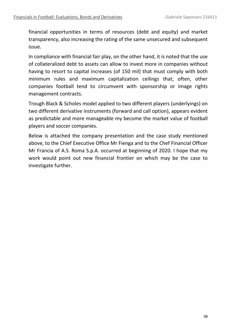
Financials in Football: Evaluations, Bonds and Derivatives - Gabriele Saponaro 216411
98
financial opportunities in terms of resources (debt and equity) and market
transparency, also increasing the rating of the same unsecured and subsequent
issue.
In compliance with financial fair play, on the other hand, it is noted that the use
of collateralized debt to assets can allow to invest more in companies without
having to resort to capital increases (of 150 mil) that must comply with both
minimum rules and maximum capitalization ceilings that, often, other
companies football tend to circumvent with sponsorship or image rights
management contracts.
Trough Black & Scholes model applied to two different players (underlyings) on
two different derivative instruments (forward and call option), appears evident
as predictable and more manageable my become the market value of football
players and soccer companies.
Below is attached the company presentation and the case study mentioned
above, to the Chief Executive Office Mr Fienga and to the Chef Financial Officer
Mr Francia of A.S. Roma S.p.A. occurred at beginning of 2020. I hope that my
work would point out new financial frontier on which may be the case to
investigate further.
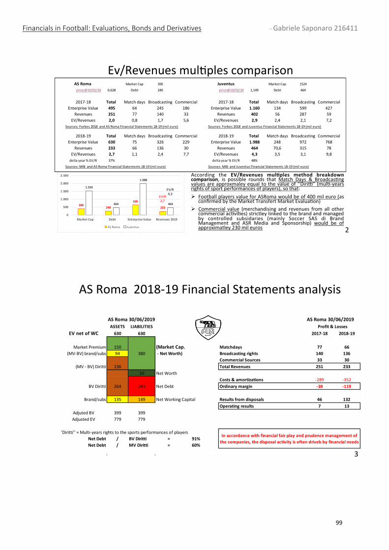
Financials in Football: Evaluations, Bonds and Derivatives - Gabriele Saponaro 216411
99
ASRoma30/06/2019 ASRoma30/06/2019
ASSETS LIABILITIES
EVnetofWC 630 630 2017-18 2018-19
MarketPremium 150 (MarketCap. Matchdays 77 66
(MV-BV)brand/subs 94 380 -NetWorth) Broadcastingrights 140 136
CommercialSources 33 30
(MV-BV)Diritti 136 TotalRevenues 251 233
10 NetWorth
Costs&amortizations -289 -352
BVDiritti 264 240 NetDebt Ordinarymargin -39 -119
Brand/subs 135 149 NetWorkingCapital Resultsfromdisposals 46 132
Operatingresults 7 13
AdjutedBV 399 399
AdjustedEV 779 779
'Diritti''=Multi-yearsrightstothesportsperformancesofplayers
NetDebt / BVDiritti = 91%
NetDebt / MVDiritti = 60%
Inaccordancewithfinancialfairplayandprudencemanagementof
thecompanies,thedisposalactivityisoftendrivebbyfinancialneeds
Profit&Losses
ASRoma2018-19FinancialStatementsanalysis
3
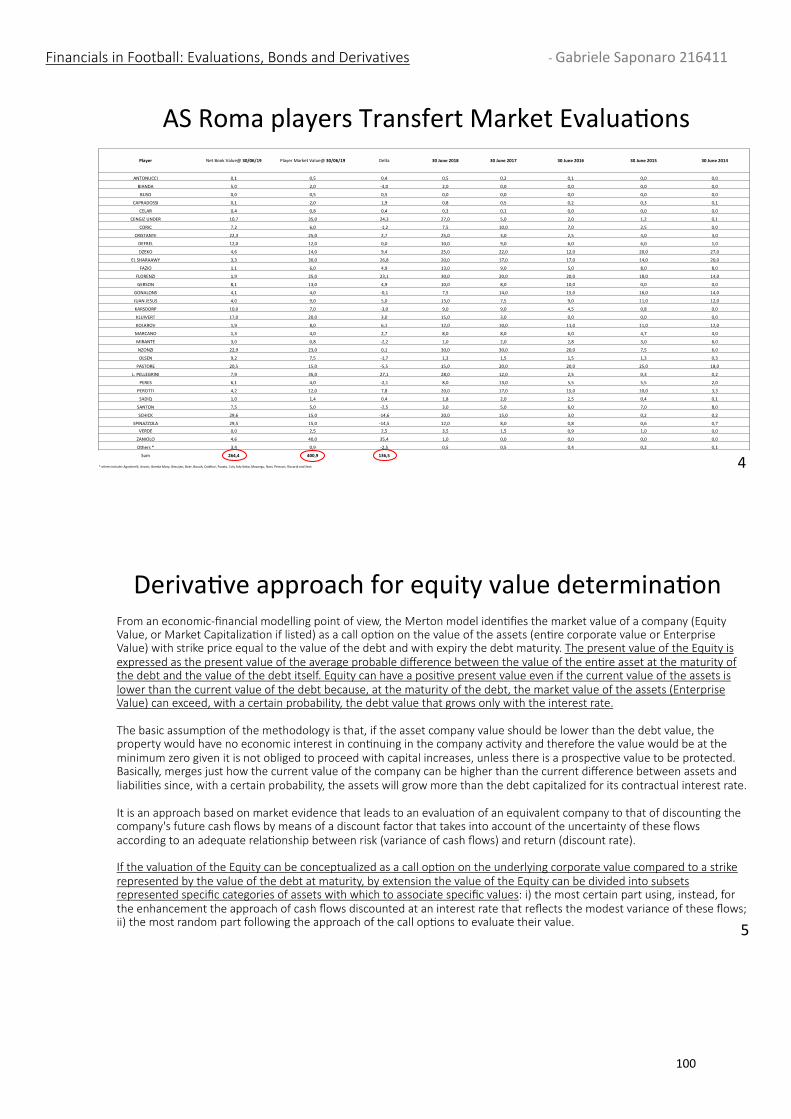
Financials in Football: Evaluations, Bonds and Derivatives - Gabriele Saponaro 216411
100
Financials in Football: Evaluations, Bonds and Derivatives - Gabriele Saponaro 216411
101
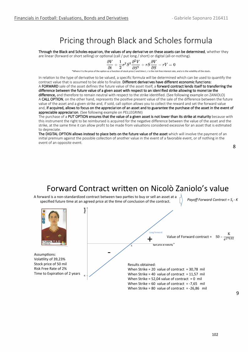
Financials in Football: Evaluations, Bonds and Derivatives - Gabriele Saponaro 216411
102
Through the Black and Scholes equa on, the values of any deriva ve on these assets can be determined, whether they are linear (forward or short selling) or op onal (call / put long / short) or digital (all-or-nothing). In rela on to the type of deriva ve to be valued, a specific formula will be determined which can be used to quan fy the contract value that is assumed to be able to finalize. Different deriva ves have different economic func ons: A FORWARD sale of the asset defines the future value of the asset itself, a forward contract lends itself to transferring the difference between the future value of a given asset with respect to an iden fied strike allowing to mone ze the difference, and therefore to remain neutral with respect to the strike iden fied. (See following example on ZANIOLO) A CALL OPTION, on the other hand, represents the posi ve present value of the sale of the difference between the future value of the asset and a given strike and, if sold, call op on allows you to collect the reward and set the forward value and, if acquired, allows to focus on the apprecia on of an asset and to guarantee the purchase of the asset in the event of appreciable apprecia on. (See following example on PELLEGRINI) The purchase of a PUT OPTION ensures that the value of a given asset is not lower than its strike at maturity because with this instrument the right to be reimbursed is acquired for the nega ve difference between the value of the asset and the strike, at the same me it can allow profit to be made from valua ons considered excessive for an asset that is es mated to depreciate. The DIGITAL OPTION allows instead to place bets on the future value of the asset which will involve the payment of an ini al premium against the possible collec on of another value in the event of a favorable event, or of nothing in the event of an opposite event.
Pricing through Black and Scholes formula
8
*WhereVisthepriceoftheop onasafunc onofstockpriceSand met,ristherisk-freeinterestrate,andσisthevola lityofthestock.
ForwardContractwri enonNicolòZaniolo’svalueAforwardisanon-standardizedcontractbetweentwopar estobuyorsellanassetata
specifiedfuture meatanagreedpriceatthe meofconclusionofthecontract. PayoffForwardContract=St-K
Assump ons:Vola lityof39,23%Stockpriceof50milRiskFreeRateof2%TimetoExpira onof2years
Resultsobtained:WhenStrike=20valueofcontract=30,78milWhenStrike=40valueofcontract=11,57milWhenStrike=52,04valueofcontract=0milWhenStrike=60valueofcontract=-7,65milWhenStrike=80valueofcontract=-26,86mil
ValueofForwardcontract=+
-
9
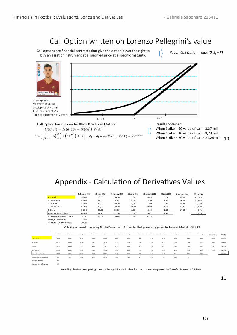
Financials in Football: Evaluations, Bonds and Derivatives - Gabriele Saponaro 216411
103
Call Op on wri en on Lorenzo Pellegrini’s value PayoffCallOp on=max(0,St–K)
Callop onsarefinancialcontractsthatgivetheop onbuyertherighttobuyanassetorinstrumentataspecifiedpriceataspecificmaturity.
K St>KSt<K
CallOp onFormulaunderBlack&ScholesMethod:
Assump ons:Vola lityof36,4%Stockpriceof40milRiskFreeRateof2%TimetoExpira onof2years
Resultsobtained:WhenStrike=60valueofcall=3,37milWhenStrike=40valueofcall=8,73milWhenStrike=20valueofcall=21,26mil, ,
10
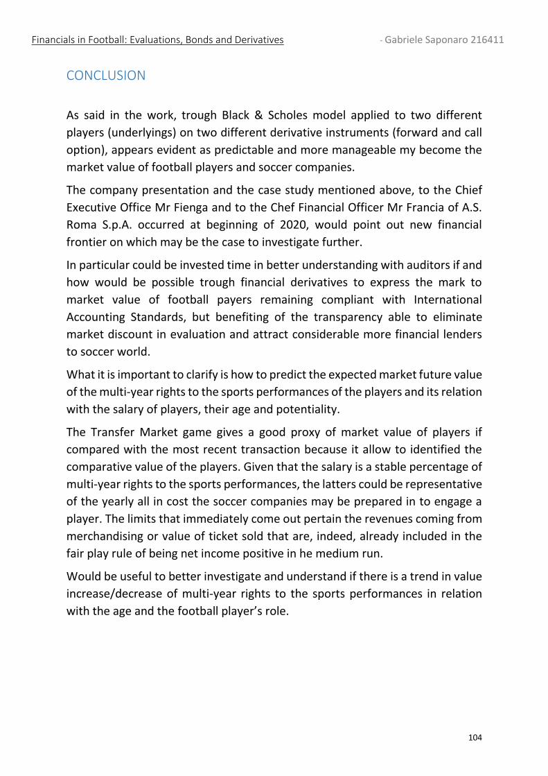
Financials in Football: Evaluations, Bonds and Derivatives - Gabriele Saponaro 216411
104
CONCLUSION
As said in the work, trough Black & Scholes model applied to two different
players (underlyings) on two different derivative instruments (forward and call
option), appears evident as predictable and more manageable my become the
market value of football players and soccer companies.
The company presentation and the case study mentioned above, to the Chief
Executive Office Mr Fienga and to the Chef Financial Officer Mr Francia of A.S.
Roma S.p.A. occurred at beginning of 2020, would point out new financial
frontier on which may be the case to investigate further.
In particular could be invested time in better understanding with auditors if and
how would be possible trough financial derivatives to express the mark to
market value of football payers remaining compliant with International
Accounting Standards, but benefiting of the transparency able to eliminate
market discount in evaluation and attract considerable more financial lenders
to soccer world.
What it is important to clarify is how to predict the expected market future value
of the multi-year rights to the sports performances of the players and its relation
with the salary of players, their age and potentiality.
The Transfer Market game gives a good proxy of market value of players if
compared with the most recent transaction because it allow to identified the
comparative value of the players. Given that the salary is a stable percentage of
multi-year rights to the sports performances, the latters could be representative
of the yearly all in cost the soccer companies may be prepared in to engage a
player. The limits that immediately come out pertain the revenues coming from
merchandising or value of ticket sold that are, indeed, already included in the
fair play rule of being net income positive in he medium run.
Would be useful to better investigate and understand if there is a trend in value
increase/decrease of multi-year rights to the sports performances in relation
with the age and the football player’s role.
Financials in Football: Evaluations, Bonds and Derivatives - Gabriele Saponaro 216411
105
Bibliography
ABI (Associazione Bancaria Italiana), Aggiornamenti sul progetto di riforma dello IAS 39: costo ammortizzato ed impairment, Documento IAS-ABI BlueBook, n.97
Baselice and Musilli, (2015) Calcio e merchandising: Italia superata dalla Francia. Nike batte Adidas, ma nel 2015.
Berardi (http://www.sportbusinessmanagement.itJ20 15/10 and Venturini (2009) ‘La Valutazione delle Performance Sportive: il Progetto FCI (Fabio Capello Index)', Rivista di Diritto ed Economia dello Sport, V (3), pp. 69-91.
Berselli, IFRS 9 in aggiornamento: novità su passività finanziarie e own credit risk, “Amministrazione & Finanza”, 2013, n.1: 35 - 38
Berselli, IFRS 9: il nuovo impairment test delle attività finanziarie, “Amministrazione & Finanza”, 2013, n.8: 21 - 26
Bertsekas and Tsistiklis. Introduction to probability. Athena Scientific, 2002.
Bjor, Arbitrage Theory in Continuous Time. Oxford Finance 2009.
Branz, Strumenti finanziari: dallo IAS 39 all’IFRS 9, “Guida alla contabilità e bilancio”, 2013, n.7: 54 – 58
Calandro, The IASB exposure draft on impairment of financial assets: a final solution or the prelude of the next credit crunch?, “Rivista dei dottori commercialisti”, 2010
Celenza, L’esposizione in bilancio degli strumenti finanziari secondo il modello IASIFRS,
Ciabattini, (20 II) Vincere con il fair play finanziario. I grandi club del calcio europeo e la nuova normativa UEFA: La fine dell’era dei mecenati (https://it.wikipedia.org/wiki/ Comitato_Olimpico_Nazionale_Italiano)
CONI (2012) “Il Libro Bianco dello Sport Italiano”. Calcio e diritti tv, perché la Spagna si adegua al resto d'Europa
Coombs, Hoppe, Pitarakis, Giovannozzi, Weissbrod, Calanni, Thissen, Kudacki, Laporta, and Byme (20 15) Commercial breaks football money league (Http://www2.deloitte.com)
Deloitte (20 15) Annual Review of Football Finance 2015
Deloitte (20 15) Football Money League 2015
Deloitte (20 16) Football Money League 2016
Deloitte (20 17) Football Money League 2017
Financials in Football: Evaluations, Bonds and Derivatives - Gabriele Saponaro 216411
106
Deloitte (20 18) Football Money League 2018
Deloitte (20 19) Football Money League 2019
Derman. Highly recommended introduction to the volatility smile problem: http://finmath.stanford.edu/seminars/documents/Stanford.Smile.Derman.pdf
Di Lazzaro, (2012) 'Società di calcio italiane ed estere'
Encyclopedia of Quantitative Finance (Rama Cont editor), Wiley 2010. Various items (No arbitrage, Fundamental Theorem of Asset Pricing, Equivalence of probability measures, Option pricing, Martingale Methods, Second FTAP...).
Favino, La classificazione e la valutazione secondo IFRS 9 (revised 2010): osservazioni critiche alla luce dell’attuale crisi finanziaria internazionale. “Quaderni Monografici Rirea”, Roma, 2011, n.98
Federazione Italiana Giuoco Calcio. (https://it.wikipedia.org)
FIGC Manuale delle Licenze UEFA. (Http://www.figc.it)
Guidantoni and Innocenti, Gli strumenti finanziari tra sistema di gestione e politiche di bilancio, “Amministrazione & Finanza”, 2012, n.7: 7 - 15
http://www.bankpedia.org/index.php/it/107-italian/i/23952-ifrs-9-un-nuovo-approccio-per-gli-strumenti-finanziari-enciclopedia
http://www.iasplus.com
http://www.master-aforisma.com/formazione-finanza/lanalista-finanziario-chi-e-quanto-guadagna-e-cosa-fare-per-diventarlo
http://www.rivistadirittotributario.it/2019/09/25/passaggio-dallo-ias-39-allifrs-9-susseguente-ampliamento-talune-perdite-valutative-delloperativita-della-presunzione-legale-sussistenza-degli/
https://res.cloudinary.com/asroma2production/image/upload/v1572449316/asroma2-prod/assets/Bilancio_AS_Roma_2019_web.pdf
https://www.asroma.com/it/club/corporate/bilanci-e-relazioni
https://www.bloomberg.com/quote/ASR:IM
Iannucci, Principi Contabili - IAS 39: strumenti finanziari derivati, “Guida alla contabilità e bilancio”, 2007, n.10: 60 – 65
Iannucci, Principi Contabili – Strumenti finanziari: attività detenute fino a scadenza, “Guida alla contabilità e bilancio”, 2007, n.20: 57 – 61
IASB, IAS 32: Strumenti finanziari: Esposizione nel bilancio.
IASB, IAS 39: Strumenti finanziari: Rilevazione e valutazione.
Financials in Football: Evaluations, Bonds and Derivatives - Gabriele Saponaro 216411
107
KPMG (2011), Le banche e la grande crisi: risultati e nuove priorità, Analisi dei Bilanci Bancari
KPMG (2010), First Impression: Additions to IFRS 9 Financial Instruments
Lapeyre, Notes on Monte Carlo Simulation, available at the linkhttp://cermics.enpc.fr/ bl/Halmstad/monte-carlo/lecture-1.pdf
Legge Beckham. (https://il.wikipedia.org/wiki/Legge_Beckham)
Paolucci and Menicucci, Novità sulla classificazione degli strumenti finanziari: l’IFRS 9, “Contabilità finanza e controllo”, 2010, n.1: 14 – 21
Parbonetti, I principi contabili internazionali: immobilizzazioni e strumenti finanziari, Carocci, 2010
Parisotto, IAS 39: un principio contabile tormentato, “Fiscalità internazionale”, 2010, vol.8, n.2: 99 - 108
Pisapia, (2012) Spagna, gli aiuti dell'Unione Europea per risanare i debiti delle squadre di calcio
Potito and Tartaglia, Polcini, I principi contabili internazionali: riflessioni critiche, in Rivista dei Dottori Commercialisti, n.2/2010
Pozzoli, Principi Contabili: Strumenti finanziari tra IAS 39 e IFRS 9, “Guida alla contabilità e bilancio”, 2010, n.2, 46 – 50
Pozzoli, Principi IAS/IFRS ed esposizione in bilancio degli strumenti finanziari, “Guida alla contabilità e bilancio”, 2012, n.5, 65 - 71
Ragaglini, “Business e Valutazione delle Performance delle Società di Calcio”
Real Madrid (2017) Management Report & Financial Statements
Reali, (2013) “L’Evoluzione del Bilancio di Esercizio delle Società di Calcio, dal Dilettantismo al Fair Play Finanziario”
Rocca, L’IFRS 9 frena i guadagni da valutazione del debito, “Norme e tributi”, 2010, Roscini Vitali F., OIC: Guide operative IAS/IFRS, Il Sole 24 Ore, 2008
Rossi, Il concetto di fair value e la valutazione degli strumenti finanziari, Milano, Giuffrè, 2003
Rutigliano, “Il Bilancio della banca e degli altri intermediary finanziari”
Santesso and Sostero, I principi contabili per il bilancio d’esercizio, Il Sole 24 Ore, 2011
Scaffa, (2014) 'La Regolamentazione del Sistema Calcio: Introduzione del FairPlay Finanziario'
Financials in Football: Evaluations, Bonds and Derivatives - Gabriele Saponaro 216411
108
Shreve (2010), Stochastic Calculus for Finance II: Continuous-Time Models. Springer Finance
Silva, Speciale bilancio IAS – IAS 39: Strumenti finanziari, “Guida alla contabilità e bilancio”, 2008, n.4: 24 – 31
Sue Lloyd IFRS 9: A Complete Package for Investors
Tari, (2013) I dati della Lega Calcio sulla tifoseria italiana di Serie A
The evolving European model of professional sports finance (2011)
Toselli and Rota, IFRS Principi Contabili internazionali: gli strumenti finanziari, 2007
Uncalcioalleconomia (2016) Chelsea leader nella massimizzazione dei profitti dei posti a sedere allo stadio. https://uncalcioalleconomia. wordpress.coml20 16
Vergani, Speciale bilancio IAS- IAS 39 – strumenti finanziari, “Guida alla contabilità e bilancio”, 2010, n.3: 35 – 42
Vulpiani, (1999) “Sviluppo di Business Plan in termini di Valore”, Analisi Finanziaria. Vulpiani, (2003) “Considerazioni sul Metodo di Valutazione Adjusted Present Value”, Revisione Contabile Vulpiani, (2004) “Elementi di Considerazione sul Processo di Valutazione delle Operazioni di M&A”, Analisi Finanziaria Vulpiani, (2006), “Cost of Capital and Valuation of Merging and Acquisition Operations” Vulpiani, (2008), “Purchase Price Allocation and choice of the Valuation Methods”, Business Valuation Review Vulpiani, (2014),“Cost Of Capital In The M&A Context: A Focus On Its Computation In Leveraged Buyout Transactions” Wilmott and Wilmott Introduces Quantitative Finance. The Wiley Finance Series 2007
www.borsaitaliana.it