November 21 2017

Financial Spillovers and Macroprudential Policies

Joshua Aizenman*, Menzie D. Chinn†, Hiro Ito‡

USC and NBER; UW-Madison and NBER; Portland State University

Abstract

We investigate whether and to what extent macroprudential policies affect the financial link between the center economies (CEs, i.e., the U.S., Japan, and the Euro area), and the peripheral economies (PHs). We first estimate the correlation of the policy interest rates between the CEs and the PHs and use that as a measure of financial sensitivity. We then estimate the determinants of the estimated measure of financial sensitivity as a function of country-specific macroeconomic conditions and policies. The potential determinant of our focus is the variable that represents the extensity of macroprudential policies. From the estimation exercise, we find that a more extensive implementation of macroprudential policies would lead PHs to (re)gain monetary independence from the CEs when the CEs implement expansionary monetary policy; when PHs run current account deficit; when they hold lower levels of international reserves (IR); when their financial markets are relatively closed; when they are experiencing an increase in net portfolio flows; and when they are experiencing credit expansion.

                                                            * Aizenman: Dockson Chair in Economics and International Relations, University of Southern California,

University Park, Los Angeles, CA 90089-0043. Phone: +1-213-740-4066. Email: aizenman@usc.edu. † Chinn: Robert M. La Follette School of Public Affairs; and Department of Economics, University of

Wisconsin, 1180 Observatory Drive, Madison, WI 53706. Phone: +1-608-262-7397. Email: mchinn@lafollette.wisc.edu .

‡ Ito (corresponding author): Department of Economics, Portland State University, 1721 SW Broadway, Portland, OR 97201. Tel/Fax: +1-503-725-3930/3945. Email: ito@pdx.edu .

Acknowledgements: The financial support of faculty research funds of University of Southern California, the University of Wisconsin, Madison, and Portland State University is gratefully acknowledged. We would like to thank Linda Goldberg for useful comments. All remaining errors are ours. Any errors are ours.

 

1  

1. Introduction

The Global Financial Crisis of 2008 led many countries, including both advanced and

developing ones, to face many policy challenges. In the aftermath of the crisis, with the hope of

jumpstarting moribund economies, policy makers in the advanced economies, or the center

economies (CEs), have implemented, sometimes experimentally, policies that had been deemed

as unconventional such as the zero or negative interest rate policy and quantitative easing (QE).

The lax monetary environment of the advanced economies caused an influx of capital

from low-yielding CEs to high-yielding emerging markets in the peripheries (PHs), bringing

about a rise in capital inflows and currency appreciation pressure for the latter. Soon after the

United States economy started showing signs of recovery in the early 2010s, however, the tide

started turning around. In 2013, a mere mention by then Federal Reserve Board (FRB) chairman,

Ben Bernanke, of the possibility of tapering off QE sent jitters to the emerging currency and

bond markets (“taper tantrum”). As the U.S. Fed did actually start tightening monetary policy

with the halt of QE in 2014 followed by the lift of the zero interest rate policy in 2015, capital

flows started flowing back to the U.S. and other advanced economies, leading to the expectation

of U.S. dollar appreciation and the depreciation of emerging market currencies. As the currencies

became expected to get weaker, the perceived level of risk among EMEs rose because many of

the firms in those economies were indebted in the dollar, which meant the debt burden would

rise as the dollar appreciates.

This development of international macroeconomic events indicates how open emerging

market economies are vulnerable to changes in the external environment, especially the financial

conditions in the CEs. This background led the “global financial cycles” view by Rey (2015) to

become widely debated. According to this view, exchange rate regimes no longer insulate

countries from global financial cycles. Financial globalization has made countries’

macroeconomic conditions more sensitive to the “global financial cycles” in capital flows, asset

prices, and credit growth, so that the famous “monetary trilemma,” or just “trilemma” – countries

can only achieve the full extent of implementation in two, not all, of the three open macro policy

goals: monetary independence, exchange rate stability, and free capital mobility4 – reduces to an

                                                            4 Also see Aizenman, et al. (2010, 2011, 2013), Obstfeld (2014), Obstfeld, et al. (2005), and Shambaugh (2004) for further discussion and references dealing with the trilemma.

 

2  

“irreconcilable duo” of monetary independence and capital mobility. Consequently, restricting

capital mobility maybe the only way for non-center countries to retain monetary autonomy.

Aizenman, et al. (2016, 2017) investigated whether Rey’s view, the end of the trilemma

hypothesis, is supported by the data. They focused on how the financial conditions of – and

shocks propagated from – the CEs (i.e., the U.S., Japan, and the Eurozone) impact the economies

in the PHs. They concluded that policy arrangements based on the trilemma do affect the extent

of linkage between CEs’ and PHs’ financial conditions. In short, an obituary for the trilemma is

not needed.

While the trilemma is not dead, it is true that open economies are subject to ebbs and

flows of capital that are heavily affected by the state of economic and financial conditions of the

CEs. That means, policy makers in the PHs need to play a balancing act; while being constrained

by the trilemma, they also need to manage to prevent financial instability. As Aizenman (2017)

put it, we may now live in a world of “quadrilemma” where financial stability have been added

to the trilemma’s original policy goals. Successful navigation of the open economy quadrilemma

helps in reducing the size of the transmission of external shocks to the domestic economy, and

reducing the costs of domestic shocks. These observations explain the relative resilience of

emerging markets, especially in countries with more mature institutions, buffered by deeper

fiscal and monetary space.

In addition to, or instead of, developing mature institutions, some countries have relied on

other policies to sustain financial stability. One prime example of policies emerging market

economies recently have started adopting is macroprudential policies.5 For example, in

recognition of the sources of Korea's vulnerabilities, since June 2010, South Korea has

introduced a series of macroprudential measures aimed at building resilience against external

financial shocks, especially against its well-known vulnerability to capital flow reversals in the

banking sector and the associated disruptions to domestic financial conditions. Other emerging

market economies such as Brazil, Indonesia, Russia, and Thailand also implemented

macroprudential policies facing an influx of capital in the aftermath of the GFC.6

                                                            5 For reviews on macroprudential policies, Bank of England (2009, 2011), Cerutti, et al. (2017), Claessens (2014), Galati and Moessner (2011, 2014), IMF (2013a,b), Lim et al. (2011), Ostry, et al. (2012), and Pasricha, et al. (2017). 6 In fact, macroprudential policies predate those implemented in the aftermath of the GFC. An oft-cited example is Chile’s unremunerated Reserve Requirement (URR) on foreign borrowing. RR was also implemented by Germany and other western European countries in the 1970s to curb capital inflows. For a historical overview of regulatory attempts to control capital flows, refer to Gosh, et al. (2018).

 

3  

The recent implementations of macroprudential policies have led to a rise in the literature

that investigates the efficacy of macroprudential policies such as Buch and Goldberg (2017),

Cerutti, et al., (2015), Ghosh, et al. (2014, 2015), Lim, et al. (2011), Ostry, et al. (2012), and

many others. This paper will be an addition to this literature. We will investigate whether and to

what extent macroprudential policies affects the financial link between the CEs and the PHs.

In our previous works, we looked at the effect of trilemma policy configurations of the

PHs on several CE-PH financial links. In this study, we focus on the link between the CEs and

the PHs through policy interest rates. We are particularly interested in examining whether a set

of macroprudential instruments can be another policy tool for the PHs to remain monetary

autonomy. While developing and emerging market economies maneuver ebbs and flows of

capital that are heavily influenced by the state and policies of the CEs, macroprudential policies

may complement the traditional open macro policies such as exchange rate regimes and financial

liberalization. It is important to investigate whether and to what extent developing and emerging

market economies delink themselves from the sphere of influence of the CEs by implementing

macroprudential instruments. Finding out the effectiveness of macroprudential policy will

provide more clues on how to navigate the world of quadrilemma.

Our empirical method relies upon a two-step approach. We first investigate the extent of

sensitivity of policy interest rate while controlling for global factors. The estimation is done for

the sample period is 1986 through 2015, using monthly data and in a rolling fashion. Next, we

examine the association of these sensitivity coefficients with the extensity of macroprudential

policy implementations while controlling for country’s trilemma choices, the real and financial

linkages with the CE, the levels of institutional development, and the like.

In what follows, we present the framework of our main empirical analysis in Section 2.

Each of the two steps for the estimation is explained in this section. In Section 3, we present

empirical results for the estimations while focusing on the effect of macroprudential policies. In

Section 4, we investigate the interactive effects between macroprudential policies and

macroeconomic conditions and policies. We make concluding remarks in Section 5.

2 The Framework of the Main Empirical Analysis

We extend the same approach as followed in Aizenman et al. (2016, 2017), with special

focus on the macroprudential policies as one of the potential determinants of the financial link

 

4  

between the CEs and the PHs. As the first step, we regress the policy interest rate of the PHs on

those of the CEs while controlling for global factors. If country i has its monetary policy more

susceptible to the monetary policy of one (or more) of the CEs, the correlation of the policy

interest rates between the CEs and PHs should be significantly positive, implying a closer

linkage between the CEs and PHs, and also that the PH of concern has less of monetary

autonomy.

Once we get the estimated coefficients of the CEs’ policy interest rates, which we treat as

the variable for the degrees of financial sensitivity, as the second step, we regress the estimated

degree of sensitivity on potential determinants, including sample countries’ macroeconomic

conditions or policies, real or financial linkage with the CEs, the level of institutional

development of the countries, and the extensity of macroprudential policies. If macroprudential

policies can affect the extent of monetary independence in a way that they help economies of our

concern to retain monetary independence, the estimated coefficient should be significantly

negative.

2.1 The First-Step: Estimating Sensitivity Coefficients

The main objective of this first step estimation is to estimate the correlation of the policy

interest rates between the CEs and peripheral economy i, while controlling for global factors. We

regress the policy interest rate of peripheral economy i ( itY ) on the vector of the policy interest

rates of the three CEs, i.e., the U.S., the Euro area, and Japan, as shown in (1). We focus on the

estimated coefficient CFi which represents the extent of financial sensitivity of peripheral country

i to the three CEs: 7

it

C

c

Cit

CFit

G

g

Git

GFitFitit XZY

11

, (1)

                                                            7 We do not include China as one of the CEs. Aizenman, et al. (2016) find that despite the recent impressive rise as an economic power, China’s contribution in the financial sector still seems negligible in a historical context. Considering that the Shanghai stock market crash in the summer of 2015 and the winter of 2016 significantly affected financial markets in the U.S., Japan, and Europe, one expects that the role of China as a CE and connectivity with it will become substantial in the near future. The same kind of argument can be made about whether other large emerging market economies such as Brazil, Russia, and India can be the center economies that exert global influence. While their role as major economies in the world has been rising, we would still have to wait for future research to identify their increasing influence in the global economy.

 

5  

where GiZ is a vector of global factors.

For money market rates that represent policy short-term interest rate, using official policy

interest rates may not capture the actual state of monetary policy because all of the CEs have

implemented extremely loose monetary policy, whether conventional or unconventional one, in

the aftermath of the GFC.8 Hence, we use the “shadow interest rates” to represent a more

realistic state of liquidity availability for the three advanced economies. For the U.S. and the

Euro area, we use the shadow interest rates estimated by Wu and Xia (2014). For Japan, we use

the shadow rates estimated by Christensen and Rudebusch (2014).

We also have global factors ( GiZ ) as a group of control variables in the estimation. As the

“real” variable, we include the first principal component of oil prices and commodity prices.9 GiZ also comprises a vector of “financial” global factors, namely, the VIX index from the

Chicago Board Options Exchange as a proxy for the extent of investors’ risk aversion as well as

the “Ted spread,” which is the difference between the 3-month Eurodollar Deposit Rate in

London (LIBOR) and the 3-month U.S. Treasury Bill yield. The latter measure gauges the

general level of stress in the money market for financial institutions.

We apply the Ordinary Least Squares (OLS) method to do the estimation for each of the

sample countries which amount to about 100 countries, including advanced economies (IDC),

less developed countries (LDC), and emerging market countries (EMG) the latter of which is a

subset of LDC.10 The sample period is 1986 through 2015, using monthly data, with regressions

implemented over non-overlapping three year periods. That means that we obtain time-varying CFit across the panels. For all the estimations, we exclude the U.S. and Japan. As for the Euro

member countries, they are removed from the sample after the introduction of the euro in

January 1999 or they become member countries, whichever comes first.11

                                                            8 This is true especially after the ECB and the Bank of Japan lowered their policy rates down to zero but before they adopted negative interest rates. 9 The use of the first principal component of oil and commodity prices is to avoid multicollinearity or redundancy. 10 The emerging market countries (EMG) are defined as the countries classified as either emerging or frontier during the period of 1980-1997 by the International Financial Corporation plus Hong Kong and Singapore. 11 Endogeneity can be an issue for this type of estimation. As a robustness check, we re-estimated the first-step model by lagging the right-hand-side variables. However, it did not change the characteristics of the results (not reported). Hence, we keep the estimation method as it is. 

 

6  

2.2 The Second Step: Baseline Model

Once we estimate CFit , we regress C

Fit on a number of country-specific variables. To

account for potential outliers on the dependent variable, we apply the robust regression

estimation technique to the following estimation model.12

FitFitFitFitFitFitFitCFit uCRISISMPIINSTLINKMCOMP 6543210ˆ (2)

Here, the choice of variables is based on a wide variety of literature pertaining to

spillover effects and global synchronization of financial or macroeconomic variables. Hence, we

assume that the above estimation model takes a reduced form, rather than a structural form, by

which we can address various theoretical predictions at once, rather than relying on one

particular theory or model.

There are four groups of explanatory variables. The first group of explanatory variables is

a set of open macroeconomic policy choices ( iOMP), for which we include the indexes for

exchange rate stability (ERS) and financial openness (KAOPEN) from the trilemma indexes by

Aizenman, et al. (2013). As another variable potentially closely related to the trilemma

framework, we include the variable for IR holding (excluding gold) as a share of GDP because

we believe the level of IR holding may affect the extent of cross-country financial linkages.13

The group of macroeconomic conditions, or iMC includes inflation volatility, current

account balance, and gross national debt (as a share of GDP).

The group of the variables that reflect the extent of linkages with the center countries

(LINK) includes trade linkage, which we measure as: ipC

ipip GDPIMPLINKTR _ where

CiIMP is total imports into center economy C from country i, normalized by country i’s GDP.

LINK also includes variables for financial linkage, for which we use the ratio of bank lending

from center economy C to country i as a share of country i’s GDP.

Another variable that reflects the linkage with the major economies is the variable for the

extent of trade competition (Trade_Comp). Trade_Comp measures the importance to country i of

                                                            12 This estimation method keeps recursively down-weighting the outliers until it obtains converged estimates. 13 Aizenman, et al. (2010, 2011) show the macroeconomic impact of trilemma policy configurations depends upon the level of IR holding.

 

7  

export competition in the third markets between country i and major country C.14 A higher value

of this measure indicates country i and major economy C exports products in similar sectors so

that their exported products tend to be competitive to each other.

The fourth group is composed of the variables that characterize the nature of institutional

development (INST), namely, variables for financial development and legal development.15 For

the measure of the level of financial development, we use Svirydzenka’s (2016) “index of

financial development” which is the first principal component of two sub-indexes, one that

captures the development of financial markets (FM) and the other that reflects the development

of financial institutions (FI). Each of FM and FI is the first principal components of three

variables: “depth,” “access,” and “efficiency,” respectively.16

The variables in MC and INST are included in the estimations as deviations from the

U.S., Japanese, and Euro Area’s counterparts. The variables in vectors OMP, MC, and INST are

sampled from the first year of each three year panels to minimize the effect of potential

endogeneity or bidirectional causality.17 Also, in order to capture global common shocks, we also

include time fixed effects.18

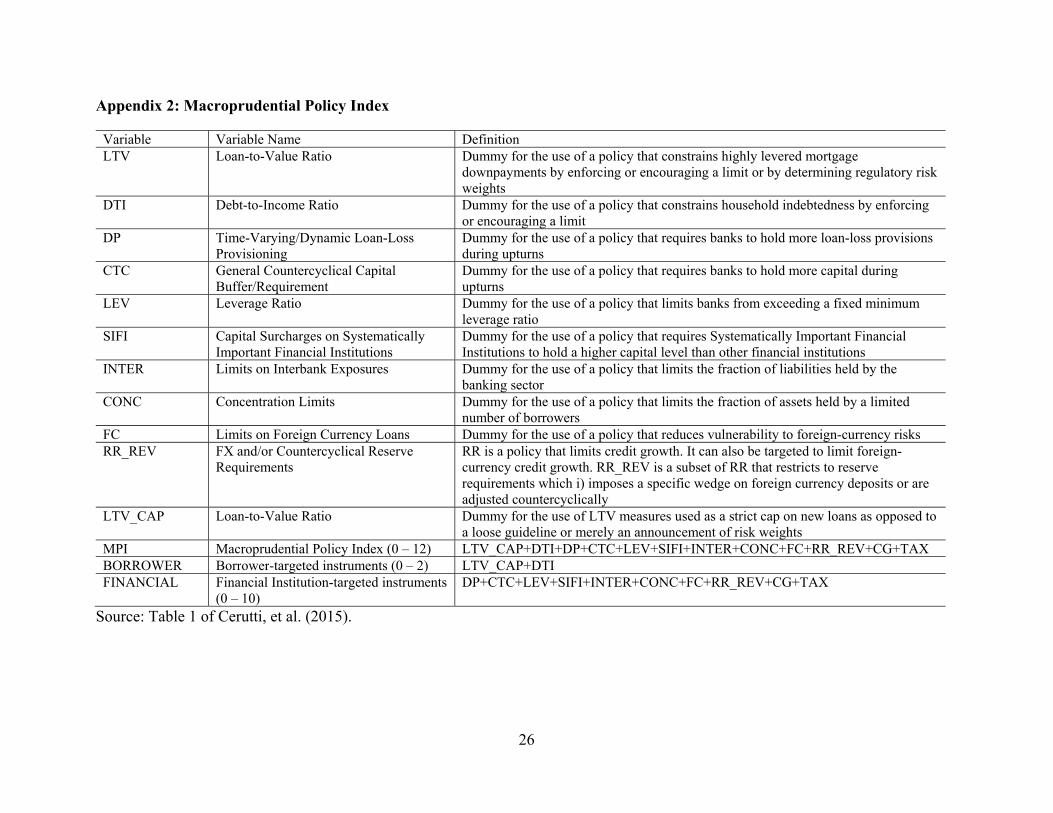
2.3 The Macroprudential Policy Index (MPI)

MPI is the variable of our focus. We assume it represents the extensity of the

implementation of macroprudential policies, for which we use the macroprudential policy dataset

developed by Cerutti, et al. (2015). This dataset is based on a comprehensive survey conducted

by the International Monetary Fund (IMF), called Global Macroprudential Policy Instruments

                                                            14 Shocks to country C, and especially shocks to country C that affects country C’s exchange rate, could affect the relative price of country C’s exports and therefore affect country i through trade competition in third markets. See Appendix 1 for the variable construction. 15 However, since the estimate of the legal development variable is found to be persistently insignificant, this variable is dropped from the estimation. 16 That is, there are FM-depth, FM-access, FM-efficiency, and FI-depth, FI-access, FI-efficiency. Each of the six sub-indexes is the first principal components of the component variables. For further details, refer to Svirydzenka (2016). 17 Sampling data from the first year of each three-year panel could still entail bidirectional causality. As another way of mitigating endogeneity or bidirectional causality, we could lag the right-hand-side variables, but by one three-year panel. Lagging the right-hand-side variables this way could mean that we assume it takes three to five years for the right-hand-side variables to affect the dependent variable, which we do not think is plausible. 18 Lastly, to control for economic or financial disruptions, we include a vector of currency and banking crises (CRISIS). For currency crisis, we use a dummy variable based on the exchange market pressure (EMP) index which is calculated using the exchange rate against the currency of the base country. The banking crisis dummy is based on the papers by Laeven and Valencia (2008, 2010, 2012).

 

8  

(GMPI). This survey sent IMF member countries’ central banks questionnaires regarding the use

and effectiveness of 18 macroprudential policy instruments. Cerruti, et al. (2015) focus on 12

policy instruments and compiled a panel dataset with dummy indicators on the usage of each

instrument for 119 countries during the period 2000-2013.

MPI is the sum of the following 12 dummies variables, each of which takes the value of

unity when the policy instrument of concern is implemented by the country.19

Loan-to-value ratio cap (LTV_CAP);

Debt to income ratio (DTI);

Dynamic Loan-loss Provision (DP);

Countercyclical capital buffer/requirement (CTC);

Leverage (LEV);

Capital surcharges on Systematically Important Financial Institutions (SIFI);

Limits on interbank exposures (INTER);

Concentration limits (CONC);

Limits on foreign currency loans (FC);

FX and/or countercyclical reserve requirements (RR_REV);

Limits on domestic currency loans (CG); and

Levy/tax on financial institutions (TAX).

We treat MPI as the measure for the extensity of macroprudential policy implementation.

Cerruti, et al. (2015) make it clear that each of the dummies does not “capture the intensity of the

measures and any changes in intensity over time.”20 Although each dummy does not directly

refer to the stringency of individual policy measures, MPI, as an aggregate of the 12 dummies,

does reflect the extensity of the macroprudential measures. To shield domestic financial markets

from the influence of external factors, countries may increase the number of macroprudential

policy instruments to make the aggregate effect stronger. Hence, extensive uses of

macroprudential policies should make the aggregate set of policy instruments more intensively

                                                            19 For more details on the dataset, refer to Appendix 2 as well as Cerruti, et al. (2015). 20 The authors also argue that codifying the degree of intensity of the measures would involve a certain degree of subjective judgements.

 

9  

effective. Therefore, the extensity of macroprudential measures should also be highly correlated

with the level of intensity of macroprudential policies.

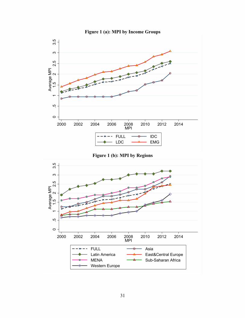
Figure 1 illustrates the development of MPI over 2000 through 2013 for different income

groups (Panel (a)) and for different regional groups (Panel (b)). We can see that the use of

macroprudential instruments is consistently becoming more frequent over years. Emerging

market economies (EMG) are the most frequent user of macroprudential policies, which is

understandable given that this group of economies are vulnerable to torrents of capital as they

liberalize their financial markets while their domestic institutions are not as highly developed as

advanced, industrial countries.

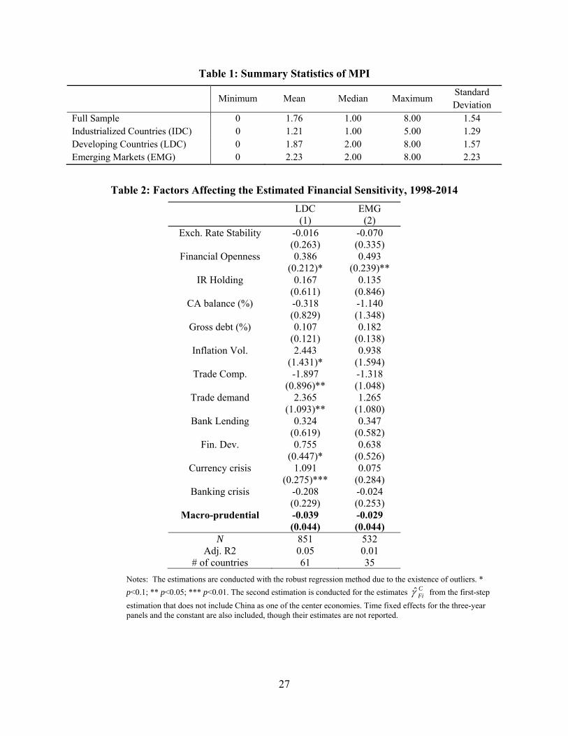
According to Table 1, both the mean and the standard deviation of MPI are the highest

for the EMG group. Industrialized countries, which as an aggregate have the lowest mean and

standard deviation in the full sample period (Table 1), increased the use of macroprudential

policies around the GFC and continued to increase the usage toward the end of the sample

period. The U.S. and European industrialized countries were the epicenters of the GFC, and

other, mostly European, industrialized countries surrounding these economies took defensive

actions to shield themselves from the shocks emanating from the epicenters. That can be

observed as rapid increases in the use of macroprudential policies by western and eastern

European economies as shown in Figure 1 (b). Among different regions, economies in Latin

America are the most frequent users of macroprudential policy instruments consistently

throughout the sample period.

These 12 dummy variables can also be categorized as those macroprudential policies

mainly representing policies that are intended to affect the behavior of borrowers (BORROWER)

and those representing policies that are intended to affect the behavior of lenders (FINANCIAL).

BORROWER is composed of loan-to-value ratio caps (LTV_CAP) and debt to income ratio

(DTI), and FINANCIAL is of LTV_CAP, DTI, DP, CTC, LEV, SIFI, INTER, CONC, FC,

RR_REV, CG, and TAX.

Using MPI, we examine whether and to what extent the implementation of

macroprudential policies, as an aggregate, affects the financial linkages between CEs and PHs.

We will also disaggregate the impact of macroprudential policies and examine whether and to

what extent borrower- or lender-based macroprudential policies affect the CE-PH links. These

variables are included in the estimation as three-year averages. Because MPI-related indexes are

 

10  

available for 2000-2013, the sample period now is composed of three-year panels start in 1998-

2000.

3 Empirical Results

3.1 First-Step Estimations – Connectivity with the CEs

As the first step, we estimate the extent of correlation of the policy interest rates between

the CEs and the PHs while controlling for two kinds of global factors: “real global” and

“financial global,” using the three-year, non-overlapping panels in the 1986-2015 period.

To gain a birds-eye view of the empirical results and the general trend of the groups of

factors that influence the financial link, we focus on the joint significance of the variables

included in the real global and financial global groups, and vector XC the latter of which includes

the policy interest rates of the CEs.

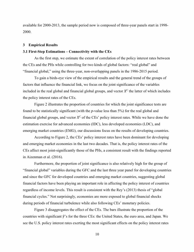
Figure 2 illustrates the proportion of countries for which the joint significance tests are

found to be statistically significant (with the p-value less than 5%) for the real global and

financial global groups, and vector XC of the CEs’ policy interest rates. While we have done the

estimation exercise for advanced economies (IDC), less developed economies (LDC), and

emerging market countries (EMG), our discussions focus on the results of developing countries.

According to Figure 2, the CEs’ policy interest rates have been dominant for developing

and emerging market economies in the last two decades. That is, the policy interest rates of the

CEs affect most joint-significantly those of the PHs, a consistent result with the findings reported

in Aizenman et al. (2016).

Furthermore, the proportion of joint significance is also relatively high for the group of

“financial global” variables during the GFC and the last three year panel for developing countries

and since the GFC for developed countries and emerging market countries, suggesting global

financial factors have been playing an important role in affecting the policy interest of countries

regardless of income levels. This result is consistent with the Rey’s (2013) thesis of “global

financial cycles.” Not surprisingly, economies are more exposed to global financial shocks

during periods of financial turbulence while also following CEs’ monetary policies.

Figure 3 disaggregates the effect of the CEs. The bars illustrate the proportion of the

countries with significant ’s for the three CEs: the United States, the euro area, and Japan. We

see the U.S. policy interest rates exerting the most significant effects on the policy interest rates

 

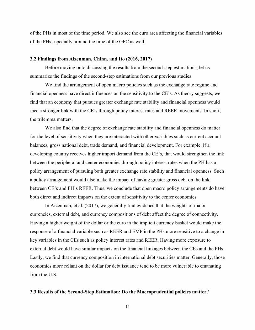
11  

of the PHs in most of the time period. We also see the euro area affecting the financial variables

of the PHs especially around the time of the GFC as well.

3.2 Findings from Aizenman, Chinn, and Ito (2016, 2017)

Before moving onto discussing the results from the second-step estimations, let us

summarize the findings of the second-step estimations from our previous studies.

We find the arrangement of open macro policies such as the exchange rate regime and

financial openness have direct influences on the sensitivity to the CE’s. As theory suggests, we

find that an economy that pursues greater exchange rate stability and financial openness would

face a stronger link with the CE’s through policy interest rates and REER movements. In short,

the trilemma matters.

We also find that the degree of exchange rate stability and financial openness do matter

for the level of sensitivity when they are interacted with other variables such as current account

balances, gross national debt, trade demand, and financial development. For example, if a

developing country receives higher import demand from the CE’s, that would strengthen the link

between the peripheral and center economies through policy interest rates when the PH has a

policy arrangement of pursuing both greater exchange rate stability and financial openness. Such

a policy arrangement would also make the impact of having greater gross debt on the link

between CE’s and PH’s REER. Thus, we conclude that open macro policy arrangements do have

both direct and indirect impacts on the extent of sensitivity to the center economies.

In Aizenman, et al. (2017), we generally find evidence that the weights of major

currencies, external debt, and currency compositions of debt affect the degree of connectivity.

Having a higher weight of the dollar or the euro in the implicit currency basket would make the

response of a financial variable such as REER and EMP in the PHs more sensitive to a change in

key variables in the CEs such as policy interest rates and REER. Having more exposure to

external debt would have similar impacts on the financial linkages between the CEs and the PHs.

Lastly, we find that currency composition in international debt securities matter. Generally, those

economies more reliant on the dollar for debt issuance tend to be more vulnerable to emanating

from the U.S.

3.3 Results of the Second-Step Estimation: Do the Macroprudential policies matter?

 

12  

We now use the estimation model based on equation (2) and investigate the determinants

of the extent of linkages through the policy interest rate, CFit , while focusing on the impact of

macroprudential policies. Table 2 reports the estimation results for the LDC and EMG samples.

Generally, compared to the results in our previous study (Aizenman, et al. 2017), the

results are unaffected despite the inclusion of the MPI in the estimation.

PHs with more open financial markets tend to follow the monetary policy of the CEs,

though the extent of exchange rate stability they pursue does not matter.21 The positive

coefficient on inflation volatility means that countries with highly volatile inflation cannot

maintain monetary independence. Those peripheral countries that export competitive products to

the CEs may be more able to delink the link of the policy interest rates with the CEs, while those

with stronger trade links with the CEs tend to have a stronger connectivity through the policy

interest rates with the CEs. The more developed financial markets a PH country is equipped

with, the more connectivity through policy interest rates it has with the CEs. This result may

reflect that countries with more developed financial markets tend to be more exposed to arbitrage

opportunities so that their interest rates tend more to be equalized or synchronized with those of

the CEs. The model, however, does not fit very well for the subsample of EMGs.

The effect of macroprudential policies on the financial link between the CEs and PHs is

not observed. Although the estimated coefficient of the MPI variable is negative for both LDCs

and EMGs, it is never statistically significant.

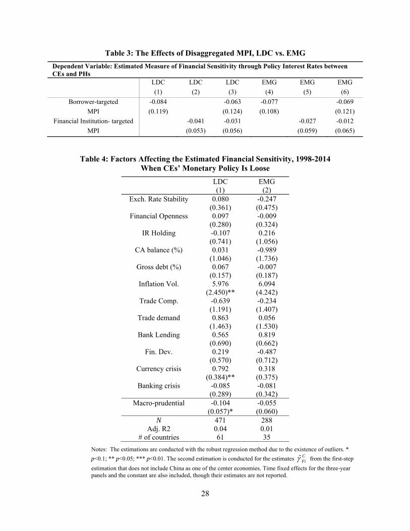
The MPI index can be disaggregated into those borrower-targeted (BORROWER) and

those targeted for financial institutions (FINANCIAL). We now replace the MPI with

BORROWER or FINANCIAL individually, or both of them together. Table 3 reports the

estimation results only for the estimates of BORROWER, FINANCIAL, or both.

Again, we do not observe any significant effect of these variables – in Table 3, neither

BORROWER nor FINANCIAL enters the estimation as a significant determinant whether the

variables are included individually or together.

Do these results suggest that macroprudential policies do not affect the financial

connectivity between the CEs and the PHs? We cannot make such a conclusion too hastily.

                                                            21 Aizenman, et al. (2017) find that the links through other financial variables are affected by the degree of exchange rate stability. Hence, unlike the “global financial cycles” argument by Rey (2013), the type of exchange rate regimes does matter.

 

13  

The effect of macroprudential policies may differ depending on the conditions of the CEs

or PHs. Macroprudential policy instruments received more attention when several important

emerging market economies such as Brazil, Korea, and Indonesia, implemented these policies

against the influx of capital caused by unconventionally lax monetary policy of the CEs. Given

that, the effectiveness of the macroprudential policies may differ whether the CEs implement a

policy that contributes to an influx of capital to the PHs or an efflux of capital from the countries.

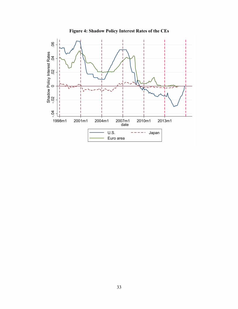
Figure 4 illustrates the shadow policy interest rates for the three CEs. From the figure, we

can see that different three-year panels (shown with vertical dotted lines) present different states

of monetary policies among the three CEs. That is, the three-year panels of 2001-03, 2007-09,

2010-12 can be clearly perceived as the periods when three CEs implemented expansionary

monetary policy which could have contributed to causing an influx of capital to emerging market

economies. In the other panels, the state of monetary policy of the three CEs appears as

contractionary or undiscernible.

From the perspective of the PHs, macroprudential policy may be more important when

the CEs relax monetary policy than otherwise, because loose monetary policy by the CEs might

necessitate PHs to take some actions against an influx of capital that is departing from the low-

yielding advanced economies for higher yields.

Now, let us estimate the variable of financial connectivity again, but this time restricting

the sample to the panels of 2001-03, 2007-09, 2010-12, i.e., the time periods when the CEs

implemented lax monetary policy. The results are reported in Table 4.

Interestingly, the estimated coefficient of the MPI becomes significantly negative for

LDC. That indicates that macroprudential policy help these economies to retain monetary

independence. In other words, macroprudential policies may help PHs to shield the influence of

the CEs’ policy interest rate changes. This evidence is consistent with the fact that many

emerging market countries implemented macroprudential policies when they experienced a rise

in capital inflows in the aftermath of the GFC. The coefficient of the MPI is also found to be

negative for the EMG subsample, but it is not statistically significant.

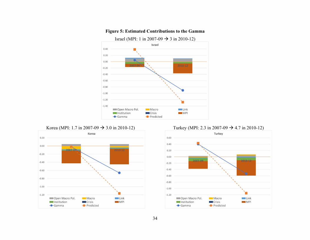
Figure 5 illustrates the contributions of the right-hand side variables to the estimated

financial sensitivity for Israel, Korea, and Turkey, using the estimates from the regression for

LDC reported in Table 4. As previously described, we group the right-hand side variables into a

group of open macroeconomic policy choices ( iOMP); macroeconomic conditions (MACRO); the

 

14  

variables that reflect the extent of linkages with the CEs (LINK); the variable that characterizes

the nature of institutional development (INST); and the MPI as the measure of the extensity of

macroprudential policies. We show the contributions of each of the groups along with the

estimated gamma from the first step regression as well as the gamma predicted from the second

step regression for the three-year panels of 2007-09 and 2010-12 – the time periods when the

CEs implement expansionary monetary policy.22

These countries represent the case where their gamma against the U.S. policy interest

rate (i.e., the estimated coefficient of the correlation between these countries’ and the U.S. policy

interest rates) fell while they increased the level of MPI. In other words, these country’s

monetary independence rose when they implemented more extensive macroprudential policies.

For example, Turkey increased the level of MPI from 2.3 in 2007-09 to 4.7 in 2010-12. The

(negative) contribution of MPI expands as the level of MPI rises while the estimated gamma

against the U.S. policy interest rate goes down from 0.40 in 2007-09 to -0.53 in 2010-12 (i.e., it

retained more monetary independence). The proportion of the MPI’s contribution, coloured in

brown, appears to be significant given the level of the gamma. Similarly, the contribution of the

MPI looks significant for both Korea and Israel, both of which experienced a fall in the estimated

gamma between the two time periods while their MPI levels went up.23 Thus, the effect of the

MPI is not just econometrically significant, but also economically significant.

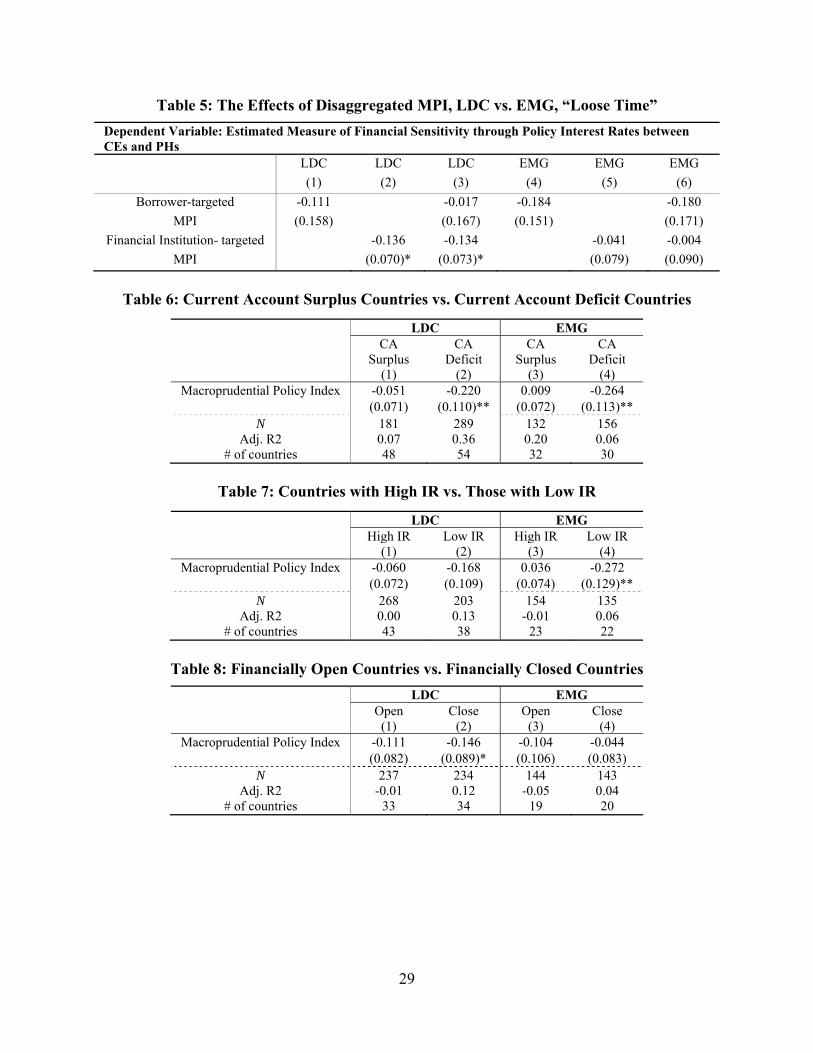
When we disaggregate the MPI into BORROWER and FINANCIAL and include them

either separately or together, the estimation results shown in Table 5 indicate that the negative

effect of the MPI variable in Table 4 come from the macroprudential policy instruments that are

targeted for lenders, i.e., financial institutions.

The above findings are not observed when the estimation is conducted for the remaining

three-year panels. These empirical findings suggest that the effect of macroprudential policy is

discernible only when the CEs implement expansionary monetary policy that eventually causes a

                                                            22 For the sake of simplicity of the graph presentation, we omit showing the contributions of the time fixed effects as well as the estimated constant. 23 As we will see in the next section, the negative correlation between the MPI and the estimated gamma is more applicable to countries running current account deficit and holding lower levels of IR. As of 2007-09 and 2010-12, Turkey ran current account deficit while Korea and Israel ran current account surplus, the latter two countries of which held relatively sizeable IR. The exercise here does not distinguish between current account surplus and deficit countries, or between high and low IR holders. Hence, we are showing the “average behavior” between these different types of economies. Economies like Korea and Israel could also implement active and preemptive macroprudential policies if they are “prudentially” afraid of the tail risk of rapid worsening of their domestic financial market conditions.

 

15  

rise in capital inflows among developing countries, but not when the CEs implement

contractionary monetary policy. In other words, the impact of macroprudential policies is

asymmetrical. That explains why we did not find a significant impact of macroprudential policies

in the baseline regression.

4. Further Analyses

We saw that macroprudential policies could affect the financial link between the CEs and

the PHs through the policy interest rates, especially when the CEs implement expansionary

monetary policy. The effect of macroprudential policies might also depend upon several other

macroeconomic or policy conditions of the PH countries that implement the policies.

Let us now examine how the effect of macroprudential policies on the financial link

might change depending on the macroeconomic or policy environment of the PHs. We test how

third factors could affect the effectiveness of macroprudential policies on the interest rate

channel between the CEs and the PHs while continuing to restrict our sample period to the

periods of CEs’ “loose” monetary policy.

First, we test the impact of current account balances. Although we observed that

macroprudential policies become effective only when the CEs implement expansionary monetary

policy, the effectiveness of macroprudential policies should differ whether the PH country of

concern is a net recipient of capital or a net lender. Historically, current account deficit countries

are more receptive to external shocks than surplus countries.

To test that, we divide the sample of LCD, or EMG, into the country-years in which the

PH runs current account surplus and those in which they run deficit. Table 4 reports the

estimation results for the MPI variable. The negative effect of macroprudential policies on the

interest rate link between CEs and PHs is observed only for current account deficit countries for

both LDC and EMG subsamples. That means that macroprudential policies allow PHs to retain

more monetary independence from the CEs when they are net recipients of capital, while

macroprudential policies do not matter for current account surplus countries.

The level of international reserves holding might matter for the effectiveness of

macroprudential policies. If a country holds a large volume of international reserves and

implement macroprudential policies, those policies may be more effective because holding a

large volume of IR could send a positive signal that the country is less vulnerable to external

 

16  

shocks. In this case, it can be argued that IR holding plays a supplemental role to

macroprudential policies. At the same time, however, macroprudential policies and IR holding

could have a substitutive relationship to each other. In that case, even if a country does not hold a

large volume of IR, active implementations of macroprudential policies might function as an

alternative buffer to external shocks.

Our estimation results suggest that macroprudential policies and IR holding have a

substitutive relationship with each other. Table 5 reports the results from the estimations in

which we divide the sample of LDC or EMG depending on the level of IR (as a share of GDP) is

greater or lower than the sample medium. According to the estimation results, for EMG countries

which do not hold high levels of IR, implementing macroprudential policies could help them

mitigate the impact of a change in the CEs’ policy interest rates on their own interest rates, i.e.,

they can retain more monetary autonomy from implementing macroprudential policies.

The impact of macroprudential policies could also depend upon the degree of openness to

international financial markets of the country that implements the policies. We divide the sample

into two subsamples depending on whether our measure of capital account openness (the Chinn-

Ito index) is above or below the sample medium and rerun the estimations. In Table 6, we

observe that macroprudential policies could be more effective when the economy of concern is

relatively financially closed. This means that when a PH country tries to shield itself from capital

inflows diverted from the CEs, having more closed financial markets would help for the

macroprudential policies to be more effective. Conversely, for PH economies with more open

financial markets, macroprudential policies would not be sufficient to manage capital inflows.

The purpose of implementing macroprudential policies is to shield the influence of

policy changes made by the CEs so that the country that implements the policies could retain its

own monetary autonomy. We have seen that PHs’ macroprudential policies are effective when

the CEs implement expansionary monetary policy. In such a situation, a lax monetary

environment among the CEs would cause capital to flow into emerging market economies with

higher yields, which could cause credit to expand in the latter. Monetary policy makers of the

PHs might become concerned that increased credit in their economies might become out of

controls, against which policy makers may implement macroprudential policies. Given this, the

effect of macroprudential policies may be more discernable when the PH economy of concern is

experiencing an increase in capital inflow and also an expansion of credit.

 

17  

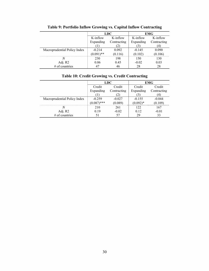
Table 9 divides the sample depending on the portfolio net inflow (as a share of GDP) is

experiencing a positive or negative growth. The coefficient of the MPI is negative for the LDC

sample for the economies that are experiencing growth in net portfolio inflows. The estimated

coefficient of the MPI for the EMG group is also negative, but only marginally significant (p-

value = 16%). Macroprudential policies are discernably effective when the PHs are experiencing

an increase in portfolio net inflows.

In Table 10, we divide the sample depending on whether the country of concern is

experiencing a growth of credit higher than its own median or not.24 The MPI variable enters the

estimation for both the LDC and EMG subsample with a significantly negative coefficient.

Taken together with the results of Table 9, we can conclude that macroprudential policies can

become effective when the CEs implement expansionary monetary policy, that causes a rise in

portfolio net inflows and credit expansion in the PHs.

5. Concluding Remarks

The implementation of unconventional monetary policies by the advanced economies in

the aftermath of the GFC significantly affected capital flows globally. Encountering a surge of

capital flows, many emerging market economies faced the need to maneuver macroeconomic

policy so as to alleviate the impacts of spillovers from the advanced economies. One such

example is macroprudential policies, which were put in place by many emerging market

economies as an attempt to mitigate the impact of changes in cross-border capital flows on

domestic financial markets and to prevent financial instability. In this paper, we empirically

investigated how the financial link through policy interest rates between the CEs and PHs can be

affected by the implementation of macroprudential policies by the PHs.

We utilized the investigation framework we used in our previous works to examine the

determinants of the financial link (Aizenman, et al. 2016, 2017) and examined whether and to

what extent a set of macroprudential policies affect the extent of sensitivity through policy

interest rates between the center, advanced economies (i.e., the U.S. the euro area, and Japan)

and developing and emerging market countries in the peripheries.

From the baseline estimation exercise, at a first glance, we found that the extensity of

macroprudential policies (measured by the macroprudential policy index, MPI) does not affect

                                                            24 We measure credit growth as a percentage growth of liquid liabilities as a share of GDP.

 

18  

the degree of connectivity through the policy interest rates between the CEs and the PHs. When

we investigated the impact of the disaggregated macroprudential policies, still, its impact on the

BE-PH link through the policy interest rates was not evidenced.

However, when we focused on the time periods when the CEs implement expansionary

monetary policy, we found that macroprudential policies do matter and negatively affect the

interest rate connectivity between the CEs and the PHs. This finding suggests that

macroprudential policies have an asymmetrical effect that arises only when CEs’ lax monetary

policy causes capital to flow to the PHs. We also found that the above negative impact of MPI is

mainly driven by lender-targeted macroprudential policies.

The effectiveness of macroprudential policies can vary depending on the macroeconomic

conditions or policies of the PH economies that implement them. Hence, we examined whether

and how macroeconomic conditions and policies could affect the effectiveness of

macroprudential policies.

We found that PH countries’ policy interest rates could become more independent of

CEs’ when macroprudential policies are implemented by the countries with current account

deficit. In other words, macroprudential policies could work more effectively for countries that

import capital from overseas.

When we compare high IR holding countries with low IR holding ones, the estimated

coefficient of the variable for macroprudential policies was found to be significantly negative,

i.e., weakening the policy interest rate link between the CEs and the PHs, only for low IR

holders. This suggests that countries with low levels of IR holding may use macroprudential

policies as a substitute to holding high levels of IR.

When we compare the PH countries that are experiencing a rise in net portfolio inflows

with those which are not, we detected the effect of macroprudential policies only among those

with increasing net portfolio inflows. We also compared the PH countries that are experiencing

credit growth with those which are not and found that only those which are experiencing credit

growth have a significantly effect on their macroprudential policies.

Thus, we have been able to show the effect of macroprudential policies as the “fourth”

factor in the quadrilemma. It must be noted that macroprudential policies are not the same as

conventional capital controls policies. What makes macroprudential policies different from

conventional capital controls is that macroprudential policies are aimed at mitigating the balance

 

19  

sheet exposure associated with short term debt flows while typical capital controls are blunt

instruments that focus more on affecting capital flows and less on mitigating the balance sheet

exposures. That may explain our findings that the effect of macroprudential policies are detected

only when the CEs implement expansionary policy and when the PHs’ domestic credit

conditions are affected.

Clearly, it is better to use more nuanced or detailed cross-country data on

macroprudential policies, rather than relying on crude dummy variables, so that we can identify

which types of macroprudential policies are effective or ineffective under what kind of policy or

macroeconomic conditions. However, such an exercise is outside the scope of this paper. We

will tackle on this issue as one of the future research agendas.

 

20  

References:

Aizenman, Joshua and Hiro Ito. 2014. “Living with the Trilemma Constraint: Relative Trilemma

Policy Divergence, Crises, and Output Losses for Developing Countries” Journal of

International Money and Finance 49 p.28-51, (May). Also available as NBER Working

Paper #19448 (September 2013). Aizenman, Joshua, Menzie D. Chinn, and Hiro Ito. 2017. “Balance Sheet Effects on Monetary

and Financial Spillovers: The East Asian Crisis Plus 20.” Journal of International Money

and Finance, vol. 74, pages 258-282.

Aizenman, Joshua, Menzie D. Chinn, and Hiro Ito. 2016. “Monetary Policy Spillovers and the

Trilemma in the New Normal: Periphery Country Sensitivity to Core Country

Conditions,” Journal of International Money and Finance, Volume 68, November 2016,

Pages 298–330. Also available as NBER Working Paper #21128 (May 2015).

Aizenman, Joshua, Menzie D. Chinn, and Hiro Ito. 2013. “The ‘Impossible Trinity’ Hypothesis

in an Era of Global Imbalances: Measurement and Testing,” Review of International

Economics, 21(3), 447–458 (August).

Aizenman, Joshua, Menzie D. Chinn, and Hiro Ito. 2011. “Surfing the Waves of Globalization:

Asia and Financial Globalization in the Context of the Trilemma,” Journal of the

Japanese and International Economies, vol. 25(3), p. 290 – 320 (September).

Aizenman, Joshua, Menzie D. Chinn, and Hiro Ito. 2010. “The Emerging Global Financial

Architecture: Tracing and Evaluating New Patterns of the Trilemma Configuration,”

Journal of International Money and Finance 29 (2010) 615–641.

Bank of England. 2011. “Instruments of Macroprudential Policy,” Bank of England Discussion

Paper (December).

Bank of England. 2009. “The Role of Macroprudential Policy,” Bank of England Discussion

Paper (November).

Buch, C. and L. Goldberg. 2017. Cross-Border Prudential Policy Spillovers: How Much? How

Important? Evidence from the International Banking Research Network, International

Journal of Central Banking, March Issue, p. 505 – 558.

Cerutti, E, S Claessens, and L Laeven. 2017. “The Use and Effectiveness of Macroprudential

Policies: New Evidence,” Journal of Financial Stability, vol. 28(C), pages 203-224.

 

21  

Cerutti, E, S Claessens, and L Laeven. 2017. “Changes in Prudential Policy Instruments – A

New Cros-country Database,” International Journal of Central Banking, vol. 13 (1), pp.

477-503, 2017.

Christensen, J. H. E., and Glenn D. Rudebusch. 2014. “Estimating Shadow-rate Term Structure

Models with Near-zero Yields,” Journal of Financial Econometrics 0, 1-34.

Claessens, Stijn. 2014. “An Overview of Macroprudential Policy Tools,” IMF WP 14/214.

Forbes, Kristin J. and Menzie D. Chinn. 2004. “A Decomposition of Global Linkages in

Financial Markets over Time,” The Review of Economics and Statistics, August, 86(3):

705–722.

Frankel, J. and S. J. Wei. 1996. “Yen Bloc or Dollar Bloc? Exchange Rate Policies in East Asian

Economies.” In T. Ito and A Krueger, eds., Macroeconomic Linkage: Savings, Exchange

Rates, and Capital Flows, Chicago: University of Chicago Press, pp 295–329.

Galatia, Gabriele and R. Moessner. 2014. “What do we know about the effects of macroprudential

policy?” DNB Working Paper, No. 440/September 2014.

Galatia, Gabriele and R. Moessner. 2011. “Macroprudential policy – a literature review,” BIS

Working Papers No 337.

Ghosh, Atish R., Mahvash S. Qureshi, and Naotaka Sugawara. 2014. “Regulating Capital Flows at

Both Ends: Does it Work?” IMF Working Paper WP/14/188. Washington, D.C.: International

Monetary Fund.

Ghosh, Atish R., Jonathan D. Ostry, and Mahvash S. Qureshi. 2015. “Exchange Rate Management

and Crisis Susceptibility: A Reassessment.” IMF Economic Review 63 (1): 238–276.  

Ghosh, Atish, Mahvash Qureshi, Jonathan Ostry, and Chifundo Moya. 2018. Managing Capital

Market Flows. Cambridge: MIT Press.

Glati, G. and R. Moessner. 2014. “What Do We Know about the Effects of Financial

Macroprudential Policy?” De Nederlandsche Bank Working Paper 440.

Glati, G. and R. Moessner. 2011. “Macroprudential Policy – A Literature Review” BIS Working

Papers 337, Bank for International Settlements.

Haldane, A. and S. Hall. 1991. “Sterling’s Relationship with the Dollar and the Deutschemark:

1976–89.” Economic Journal, 101:406 (May).

Hausmann, R. and Panizza, U., 2011. “Redemption or abstinence? original sin, currency

mismatches and counter cyclical policies in the new millennium,” Journal of

Globalization and Development, 2(1).

 

22  

International Monetary Fund. 2013a. “Key Aspects of Macroprudential Policy,” IMF Policy

Paper (June).

International Monetary Fund. 2013b. “Key Aspects of Macroprudential Policy – Background

Paper,” IMF Policy Paper (June).

Ito, H. and M. Kawai. 2016. “|Trade invoicing in major currencies in the 1970s-1990s: lessons

for renminbi internationalization,” Journal of the Japanese and International Economies,

vol 42, December, pp 123–145.

Ito, H. and C. Rodriguez. 2015. “Clamoring for Greenbacks: Explaining the Resurgence of the

US Dollar in International Debt.” RIETI Working Paper 15-E-119 (October).

Ito, H, R. McCauley and T. Chan. 2015. “Emerging market currency composition of reserves,

denomination of trade and currency movements”, Emerging Markets Review, December,

pp 16-19.

Laeven, L. and F. Valencia. 2012. “Systematic Banking Crises: A New Database,” IMF Working

Paper WP/12/163, Washington, D.C.: International Monetary Fund.

Laeven, L. and F. Valencia. 2010. “Resolution of Banking Crises: The Good, the Bad, and the

Ugly,” IMF Working Paper No. 10/44. Washington, D.C.: International Monetary Fund.

Laeven, L. and F. Valencia. 2008. “Systematic Banking Crises: A New Database,” IMF Working

Paper WP/08/224, Washington, D.C.: International Monetary Fund.

McCauley, R. and T. Chan 2014. “Currency movements drive reserve composition”, BIS

Quarterly Review, December, pp 23-36.

Ostry, J., A. Ghosh, M. Chamon, and M. Qureshi. 2012. “Tools for Managing Financial-Stability

Risks from Capital Inflows,” Journal of International Economics, 88(2): p. 407 – 421.

Pasricha, G., M. Falagiarda, M. Bijsterbosch, and J. Aizenman. 2017. Domestic and Multilateral

Effects of Capital Controls in Emerging Markets, NBER Working Paper Series 20822.

Cambridge: National Bureau of Economic Research.

Rey, H. 2013. “Dilemma not Trilemma: The Global Financial Cycle and Monetary Policy

Independence,” prepared for the 2013 Jackson Hole Meeting.

Shambaugh, J. C., 2004. The Effects of Fixed Exchange Rates on Monetary Policy. Quarterly

Journal of Economics 119 (1), 301-52.

Wu, Jing Cynthia and Fan Dora Xia. 2014. “Measuring the Macroeconomic Impact of Monetary

Policy at the Zero Lower Bound”, NBER Working Paper No. 20117.

 

23  

 

24  

Appendix 1: Data Descriptions and Sources Policy short-term interest rate – money market rates. Extracted from the IMF’s International

Financial Statistics (IFS).

Commodity prices – the first principal component of oil prices and commodity prices, both from the IFS.

VIX index – It measures the implied volatility of S&P 500 index options and is available in http://www.cboe.com/micro/VIX/vixintro.aspx.

“Ted spread” – It is the difference between the 3-month Eurodollar Deposit Rate in London (LIBOR) and the 3-month U.S. Treasury Bill yield.

Exchange rate stability (ERS) and financial openness (KAOPEN) indexes – From the trilemma indexes by Aizenman, et al. (2013).

International reserves – international reserves minus gold divided by nominal GDP. The data are extracted from the IFS.

Gross national debt – It is included as a share of GDP and obtained from the World Economic Outlook (WEO) database.

Trade demand by the CEs – ipC

ipip GDPIMPLINKTR _ where CiIMP is total imports into center

economy C from country i, that is normalized by country i’s GDP and based on the data from the IMF Direction of Trade database.

FDI provided by the CEs – It is the ratio of the total stock of foreign direct investment from country C in country i as a share of country i’s GDP. We use the OECD International Direct Investment database.

Bank lending provided by the CEs – It is the ratio of the total bank lending provided by each of the CEs to country i shown as a share of country i’s GDP. We use the BIS database.

Trade competition – It is constructed as follows.

k i

ikW

WkW

CkWC

i GDP

Exp

Exp

Exp

CompTradeMaxCompTrade ,

,

, *)_(

100_

CkWExp , is exports from large-country C to every other country in the world (W) in industrial

sector k whereas WkWExp , is exports from every country in the world to every other country in

the world (i.e. total global exports) in industrial sector k. ikWExp , is exports from country i to

every other country in the world in industrial sector k, and GDPi is GDP for country i. We assume merchandise exports are composed of five industrial sectors (K), that is, manufacturing, agricultural products, metals, fuel, and food.

This index is normalized using the maximum value of the product in parentheses for every country pair in the sample. Thus, it ranges between zero and one.25 A higher value of this variable means that country i’s has more comparable trade structure to the center economies.

                                                            25 This variable is an aggregated version of the trade competitiveness variable in Forbes and Chinn (2004). Their index is based on more disaggregated 14 industrial sectors.

 

25  

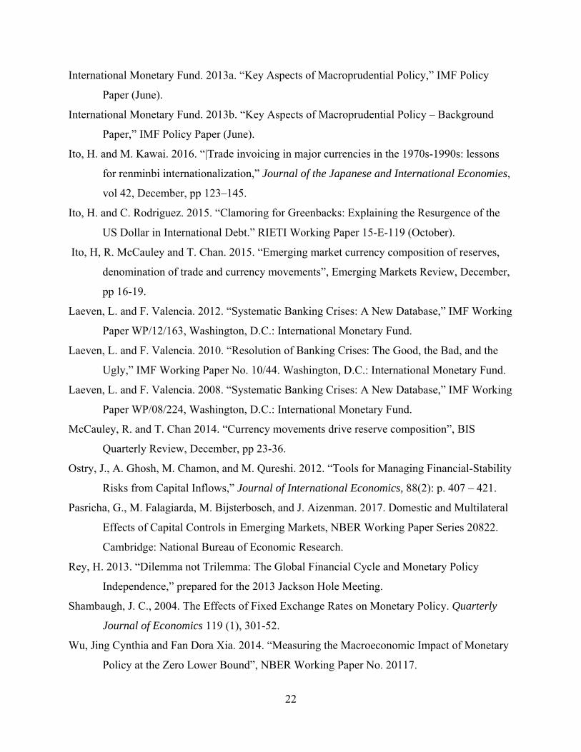
Financial development – It is the first principal component of private credit creation, stock market capitalization, stock market total value, and private bond market capitalization all as shares of GDP.26

Currency crisis – It is from Aizenman and Ito (2014) who use the exchange market pressure (EMP) index using the exchange rate against the currency of the base country. We use two standard deviations of the EMP as the threshold to identify a currency crisis. To construct the crisis dummies in three-year panels, we assign the value of one if a crisis occurs in any year within the three-year period.

Banking crisis – It is from Aizenman and Ito (2014) who follow the methodology of Laeven and Valencia (2008, 2010, 2012). For more details, see Appendix 1 of Aizenman and Ito (2014).

Share of export/import – The share of country i’s export to, or import from, a major currency country (e.g., Japan) in country i’s total export or import. The data are taken from the IMF’s Direction of Trade.

Commodity export/import as a percentage of total export/import – Data are taken from the World Bank’s World Development Indicators and the IMF’s International Financial Statistics.

                                                            26 Because the private bond market capitalization data go back only to 1990, the FD series before 1990 are extrapolated using the principal component of private credit creation, stock market capitalization, and stock market total values, which goes back to 1976. These two FD measures are highly correlated with each other.

 

26  

Appendix 2: Macroprudential Policy Index

Variable Variable Name Definition LTV Loan-to-Value Ratio Dummy for the use of a policy that constrains highly levered mortgage

downpayments by enforcing or encouraging a limit or by determining regulatory risk weights

DTI Debt-to-Income Ratio Dummy for the use of a policy that constrains household indebtedness by enforcing or encouraging a limit

DP Time-Varying/Dynamic Loan-Loss Provisioning

Dummy for the use of a policy that requires banks to hold more loan-loss provisions during upturns

CTC General Countercyclical Capital Buffer/Requirement

Dummy for the use of a policy that requires banks to hold more capital during upturns

LEV Leverage Ratio Dummy for the use of a policy that limits banks from exceeding a fixed minimum leverage ratio

SIFI Capital Surcharges on Systematically Important Financial Institutions

Dummy for the use of a policy that requires Systematically Important Financial Institutions to hold a higher capital level than other financial institutions

INTER Limits on Interbank Exposures Dummy for the use of a policy that limits the fraction of liabilities held by the banking sector

CONC Concentration Limits Dummy for the use of a policy that limits the fraction of assets held by a limited number of borrowers

FC Limits on Foreign Currency Loans Dummy for the use of a policy that reduces vulnerability to foreign-currency risksRR_REV FX and/or Countercyclical Reserve

Requirements RR is a policy that limits credit growth. It can also be targeted to limit foreign-currency credit growth. RR_REV is a subset of RR that restricts to reserve requirements which i) imposes a specific wedge on foreign currency deposits or are adjusted countercyclically

LTV_CAP Loan-to-Value Ratio Dummy for the use of LTV measures used as a strict cap on new loans as opposed to a loose guideline or merely an announcement of risk weights

MPI Macroprudential Policy Index (0 – 12) LTV_CAP+DTI+DP+CTC+LEV+SIFI+INTER+CONC+FC+RR_REV+CG+TAX BORROWER Borrower-targeted instruments (0 – 2) LTV_CAP+DTIFINANCIAL Financial Institution-targeted instruments

(0 – 10) DP+CTC+LEV+SIFI+INTER+CONC+FC+RR_REV+CG+TAX

Source: Table 1 of Cerutti, et al. (2015).

 

27  

Table 1: Summary Statistics of MPI

Minimum Mean Median Maximum

Standard Deviation

Full Sample 0 1.76 1.00 8.00 1.54 Industrialized Countries (IDC) 0 1.21 1.00 5.00 1.29 Developing Countries (LDC) 0 1.87 2.00 8.00 1.57 Emerging Markets (EMG) 0 2.23 2.00 8.00 2.23

Table 2: Factors Affecting the Estimated Financial Sensitivity, 1998-2014

LDC EMG (1) (2)

Exch. Rate Stability -0.016 -0.070 (0.263) (0.335)

Financial Openness 0.386 0.493 (0.212)* (0.239)**

IR Holding 0.167 0.135 (0.611) (0.846)

CA balance (%) -0.318 -1.140 (0.829) (1.348)

Gross debt (%) 0.107 0.182 (0.121) (0.138)

Inflation Vol. 2.443 0.938 (1.431)* (1.594)

Trade Comp. -1.897 -1.318 (0.896)** (1.048)

Trade demand 2.365 1.265 (1.093)** (1.080)

Bank Lending 0.324 0.347 (0.619) (0.582)

Fin. Dev. 0.755 0.638 (0.447)* (0.526)

Currency crisis 1.091 0.075 (0.275)*** (0.284)

Banking crisis -0.208 -0.024 (0.229) (0.253)

Macro-prudential -0.039 -0.029 (0.044) (0.044)

N 851 532Adj. R2 0.05 0.01

# of countries 61 35

Notes: The estimations are conducted with the robust regression method due to the existence of outliers. *

p<0.1; ** p<0.05; *** p<0.01. The second estimation is conducted for the estimates CFi from the first-step

estimation that does not include China as one of the center economies. Time fixed effects for the three-year panels and the constant are also included, though their estimates are not reported.

 

28  

Table 3: The Effects of Disaggregated MPI, LDC vs. EMG

Dependent Variable: Estimated Measure of Financial Sensitivity through Policy Interest Rates between CEs and PHs

LDC LDC LDC EMG EMG EMG

(1) (2) (3) (4) (5) (6)

Borrower-targeted -0.084 -0.063 -0.077 -0.069

MPI (0.119) (0.124) (0.108) (0.121)

Financial Institution- targeted -0.041 -0.031 -0.027 -0.012

MPI (0.053) (0.056) (0.059) (0.065)

 

Table 4: Factors Affecting the Estimated Financial Sensitivity, 1998-2014 When CEs’ Monetary Policy Is Loose

LDC EMG (1) (2)

Exch. Rate Stability 0.080 -0.247 (0.361) (0.475)

Financial Openness 0.097 -0.009 (0.280) (0.324)

IR Holding -0.107 0.216 (0.741) (1.056)

CA balance (%) 0.031 -0.989 (1.046) (1.736)

Gross debt (%) 0.067 -0.007 (0.157) (0.187)

Inflation Vol. 5.976 6.094 (2.450)** (4.242)

Trade Comp. -0.639 -0.234 (1.191) (1.407)

Trade demand 0.863 0.056 (1.463) (1.530)

Bank Lending 0.565 0.819 (0.690) (0.662)

Fin. Dev. 0.219 -0.487 (0.570) (0.712)

Currency crisis 0.792 0.318 (0.384)** (0.375)

Banking crisis -0.085 -0.081 (0.289) (0.342)

Macro-prudential -0.104 -0.055 (0.057)* (0.060)

N 471 288Adj. R2 0.04 0.01

# of countries 61 35

Notes: The estimations are conducted with the robust regression method due to the existence of outliers. *

p<0.1; ** p<0.05; *** p<0.01. The second estimation is conducted for the estimates CFi from the first-step

estimation that does not include China as one of the center economies. Time fixed effects for the three-year panels and the constant are also included, though their estimates are not reported.

 

29  

Table 5: The Effects of Disaggregated MPI, LDC vs. EMG, “Loose Time”

Dependent Variable: Estimated Measure of Financial Sensitivity through Policy Interest Rates between CEs and PHs

LDC LDC LDC EMG EMG EMG

(1) (2) (3) (4) (5) (6)

Borrower-targeted -0.111 -0.017 -0.184 -0.180

MPI (0.158) (0.167) (0.151) (0.171)

Financial Institution- targeted -0.136 -0.134 -0.041 -0.004

MPI (0.070)* (0.073)* (0.079) (0.090)

 

Table 6: Current Account Surplus Countries vs. Current Account Deficit Countries

LDC EMG CA

SurplusCA

DeficitCA

SurplusCA

Deficit (1) (2) (3) (4)

Macroprudential Policy Index -0.051 -0.220 0.009 -0.264 (0.071) (0.110)** (0.072) (0.113)**

N 181 289 132 156 Adj. R2 0.07 0.36 0.20 0.06

# of countries 48 54 32 30

 

Table 7: Countries with High IR vs. Those with Low IR

LDC EMG High IR Low IR High IR Low IR (1) (2) (3) (4)

Macroprudential Policy Index -0.060 -0.168 0.036 -0.272 (0.072) (0.109) (0.074) (0.129)**

N 268 203 154 135 Adj. R2 0.00 0.13 -0.01 0.06

# of countries 43 38 23 22

Table 8: Financially Open Countries vs. Financially Closed Countries

LDC EMG Open Close Open Close (1) (2) (3) (4)

Macroprudential Policy Index -0.111 -0.146 -0.104 -0.044 (0.082) (0.089)* (0.106) (0.083)

N 237 234 144 143 Adj. R2 -0.01 0.12 -0.05 0.04

# of countries 33 34 19 20

 

30  

Table 9: Portfolio Inflow Growing vs. Capital Inflow Contracting

LDC EMG K-inflow

ExpandingK-inflow

Contracting K-inflow

ExpandingK-inflow

Contracting (1) (2) (3) (4)

Macroprudential Policy Index -0.214 0.092 -0.145 0.090 (0.091)** (0.116) (0.102) (0.106)

N 230 198 150 130 Adj. R2 0.06 0.45 -0.02 0.03

# of countries 47 46 28 28

Table 10: Credit Growing vs. Credit Contracting

LDC EMG Credit

ExpandingCredit

Contracting Credit

ExpandingCredit

Contracting (1) (2) (3) (4)

Macroprudential Policy Index -0.259 -0.027 -0.155 -0.044 (0.087)*** (0.089) (0.092)* (0.109)

N 210 261 122 167 Adj. R2 0.19 -0.02 0.12 -0.01

# of countries 51 57 29 33

 

31  

Figure 1 (a): MPI by Income Groups

Figure 1 (b): MPI by Regions

0.5

11.

52

2.5

33.

5A

vera

ge M

PI

2000 2002 2004 2006 2008 2010 2012 2014MPI

FULL IDC LDC EMG

0.5

11.

52

2.5

33.

5A

vera

ge M

PI

2000 2002 2004 2006 2008 2010 2012 2014MPI

FULL Asia

Latin America East&Central Europe MENA Sub-Saharan Africa Western Europe

 

32  

Figure 2: Proportion of Significant F-Tests

CE: Policy Interest Rate PH: Policy Interest Rate

Figure 3: Proportion of Significant ’s

0.2

.4.6

.81

% o

f S

ig.

Est

imat

es

1992-19941995-1997

1998-20002001-2003

2004-20062007-2009

2010-20122013-2014

LDC Sample

Real Global Fin. GlobalCross-link

0.2

.4.6

.81

% o

f Sig

. Est

imat

es

1992-19941995-1997

1998-20002001-2003

2004-20062007-2009

2010-20122013-2014

EMG

U.S. JapanEuro

 

33  

Figure 4: Shadow Policy Interest Rates of the CEs

-.04

-.02

0.0

2.0

4.0

6S

hado

w P

olic

y In

tere

st R

ates

1998m1 2001m1 2004m1 2007m1 2010m1 2013m1date

U.S. Japan Euro area

 

34  

Figure 5: Estimated Contributions to the Gamma

Israel (MPI: 1 in 2007-09 3 in 2010-12)

Korea (MPI: 1.7 in 2007-09 3.0 in 2010-12) Turkey (MPI: 2.3 in 2007-09 4.7 in 2010-12)