FINANCIAL PLANNING WITH 0-1 KNAPSACK PROBLEMS, … · A number of branch and bound algorithms have been presented for the solution ofthe 0-1 knapsack problem. Perhaps the fIrst branch

FINANCIAL PLANNING WITH 0-1 KNAPSACK PROBLEMS, PART II: USING DOMINATION RESULTS TO SOLVE KNAPSACK PROBLEMS

Daniel E. O'Leary

ABSTRACT

Part II uses domination results in knapsack problems to assist in generating solutions more rapidly and with less work. In particular, domination results are used to: (1) generate smaller problems so that less work is needed to solve the problems, and (2) speed up solution by pruning the variable sets that must be examined. Three solution processes are examined in Part II. Domination resultS are used on branch and bound algorithms, dynamic programming algorithm and epsilon-approximate algorithms. Use of domination concepts can substantially reduce the computational demands of a solution process.

Advanees in Mathematical Programming and Financial Planning, Volume 4, pages 151-1". Copyright © 1995 hy JAI Press Ine. AU rights of reproduction in any form reserved. ISBN: 1-55'38-724-6

151

,"

152 DANIEL E. O'LEARY

VI. APPLICATION TO BRANCH AND BOUND ALGORITHMS

The domination results can be used to improve the branch and bound algorithms of Kolesar (1967) and Greenberg and Hegerich (1970), and other similar algorithms. This section extends the domination results, illustrates their use and provides some empirical evidence which illustrates the impact of incorporating the domination results in those algorithms.

A. Background

A number of branch and bound algorithms have been presented for the solution ofthe 0-1 knapsack problem. Perhaps the fIrst branch and bound algorithm was that ofKolesar (1967), who sequentially branched on each variable, Xl' x2' and so on. For each of the two branches coming out of a given node, the variable was set to 0 or I. The upper bound was then examined to determine whether or not it exceeded the best known solution up to that branch in the tree. If it did then branching continued. Ifnot branching stopped. Greenberg and Hegerich (1970) also developed a similar branch and bound algorithm to Problem (1). However, instead of branching on the variables in sequence, their approach was to branch on the one variable that was non integer in the linear programming solution to Problem (1).

In these and other algorithms, the upper bound has been determined using a linear programming solution to Problem (I). In that computation, a linear programming approach is used to solve the problem that results from the remaining variables that have not been set equal to 0 or 1 in the branching and bound tree.

B. Revisions Due to Domination

Each of those algorithms (e.g., Kolesar, 1967 and Greenberg and Hegerich, 1970) can be improved by using the reduced problem of Theorem 7 instead of the original Problem (1). In addition, those algorithms can make use of the domination results in another fashion. Let

Kl = {i I Xl is set at 1 at the node of the search tree

under consideration}

J<!l = {i I Xi is set at 0 at the node of the search tree

under consideration}

"

Financial Planning with 0-1 Knapsack Problems, Part II 153

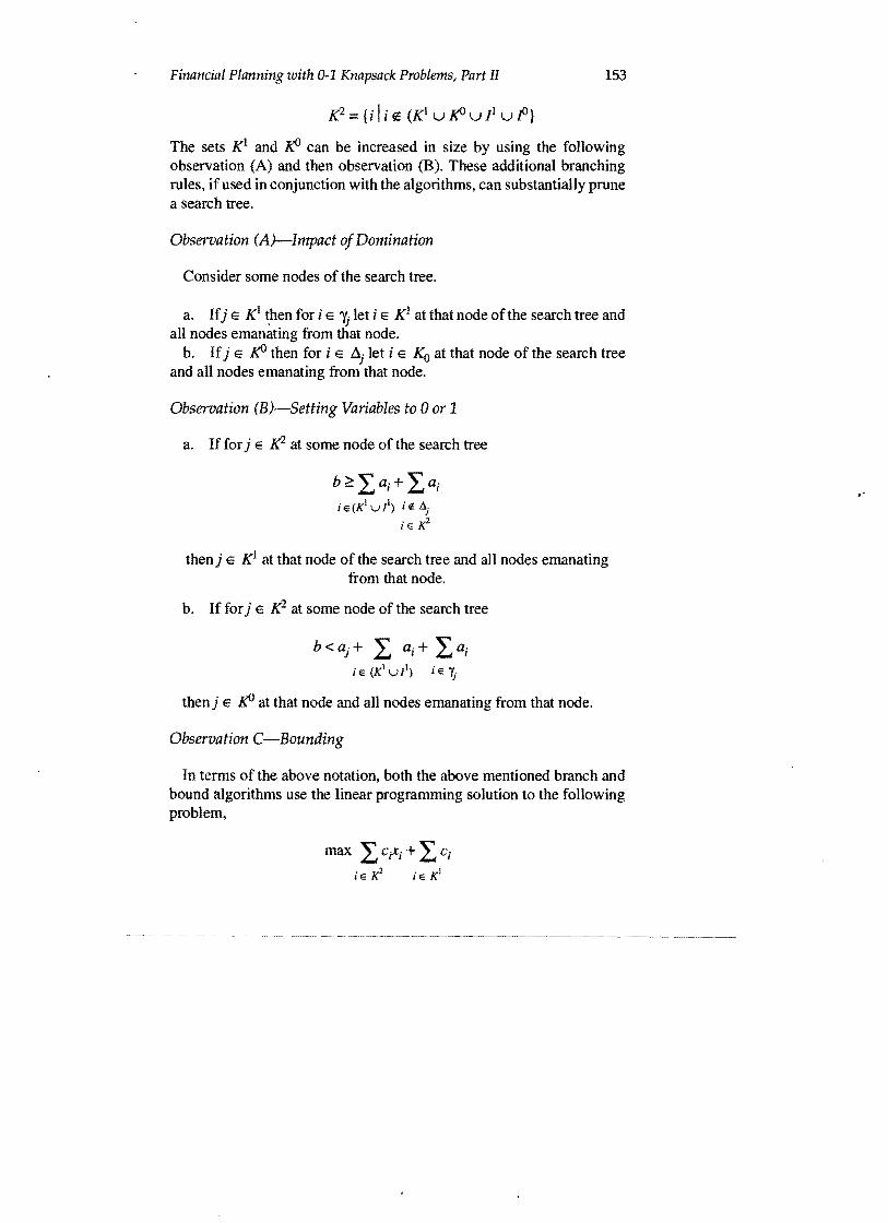
K2 ={i Ii it (K1 U f<!J U /1 U .to}

The sets KI and f<!J can be increased in size by using the following observation (A) and then observation (B). These additional branching rules, ifused in conjunction with the algorithms, can substantially prune a search tree.

Observation (A)-Impact of Domination

Consider some nodes of the search tree.

a. Ifj E KI ~hen for i E "ij let i E KI at that node ofthe search tree and all nodes emanating from that node.

b. Ifj E f<!J then for i E llj let i E Ko at that node of the search tree and all nodes emanating from that node.

Observation (B)-Setting Variables to 0 or 1

a. If for j E K2 at some node of the search tree

b~la;+ la; j E (Ki V hili! tJ.j

iE If

then j E KI at that node of the search tree and all nodes emanating from that node.

b. If for j E K2 at some node of the search tree

b < aj + 1 ai + 1 aj

iE(K1vi) iEYj

then j E f<!J at that node and all nodes emanating from that node.

Observation C-Bounding

In terms of the above notation, both the above mentioned branch and bound algorithms use the linear programming solution to the following problem,

max lCrj+ lc; j E K2 i E Kl

"


I ari =::; b - I ai

ieK- ieK1

1> >0' K2-xi _ ,I E

as a means of establishing the upper bound at a given node of the search tree. Using observations (A) and (B), that bound can be improved by using the linear programming solution to the following problem as the upper bound,

max I Cri + ICi

ie (K2 r. p) Ie (K1 v i)

If i E (K2 n p) and xi ~ Xj is in the reduced domination

network

C Example "

Consider the example in Kolesar, 1967 and Greenberg and Hegerich, 1970,

max 60xI + 60x2 + 40x3 + 10x4 + 20xs + lOx6 + 3x7

100 ~ 30xI + 50x2 + 40x3 + lOx4 + 40xs + 30x6 + lOx7

xi =0 or 1.

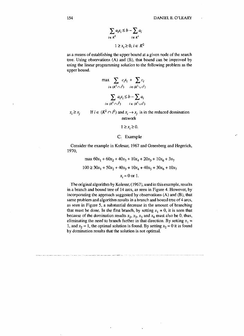
The original algorithm by Kolesar, (1967), used in this example, results in a branch and bound tree of 14 arcs, as seen in Figure 4. However, by incorporating the approach suggested by observations (A) and (B), that same problem and algorithm results in a branch and bound tree of4 arcs, as seen in Figure 5, a substantial decrease in the amount of branching that must be done. In the first branch, by setting XI =0, it is seen that because of the domination results x2' x3' Xs and x6 must also be 0, thus, eliminating the need to branch further in that direction. By setting Xl = 1, and ~ =1, the optimal solution is found. By setting x2 =0 it is found by domination results that the solution is not optimal.

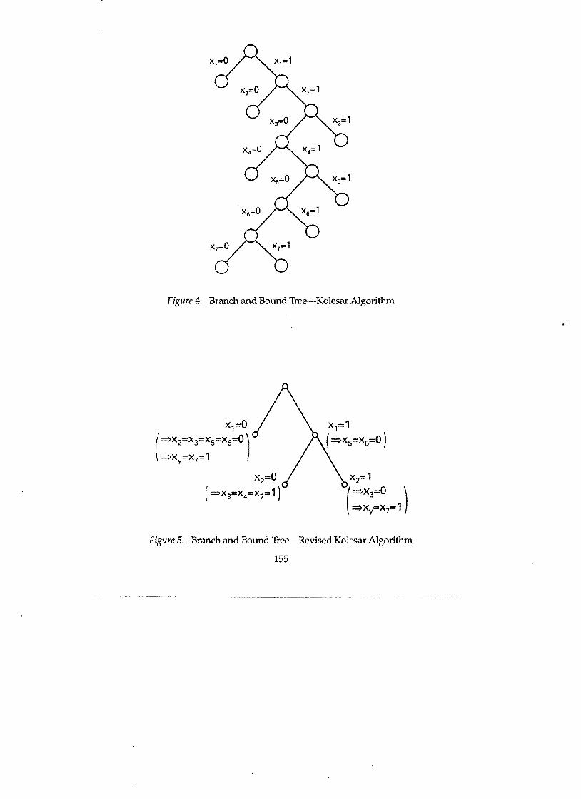
Figure 4. Branch and Bound Tree-Kolesar Algorithm

x1=o (~X2=X3=X5=X6=O1 \ ~xy;;;:x7=1

X2=O

( ~X3=X4=X7=1 )

Figure 5. Branch and Bound Tree-Revised Kolesar Algorithm

155

,"

(


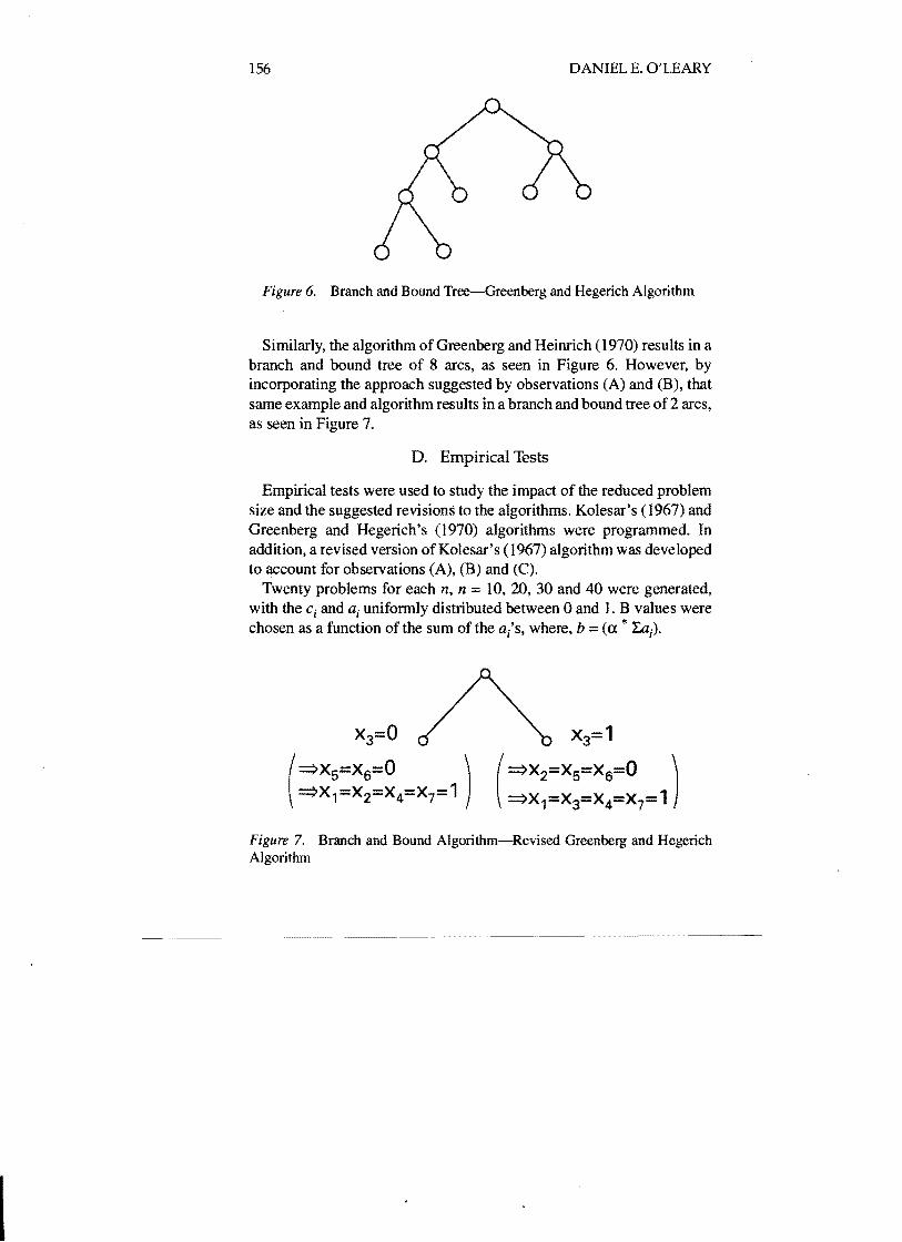
Figure 6. Branch and Bound Tree-Greenberg and Hegerich Algorithm

Similarly, the algorithm of Greenberg and Heinrich (1970) results in a branch and bound tree of 8 arcs, as seen in Figure 6. However, by incorporating the approach suggested by observations (A) and (B), that same example and algorithm results in a branch and bound tree of 2 arcs, as seen in Figure 7.

D. Empirical Tests

Empirical tests were used to study the impact of the reduced problem size and the suggested revisions to the algorithms. Kolesar's (1967) and Greenberg and Hegerich's (1970) algorithms were programmed. In addition, a revised version ofKolesar's (1967) algorithm was developed to account for observations (A), (B) and (C).

Twenty problems for each n, n == 10, 20, 30 and 40 were generated, with the cj and a j uniformly distributed between 0 and I. B values were chosen as a function ofthe sum of the a/s, where, b == (c:x * Laj ).

x3=1

==>X2=XS=X6=O )

==>X1=X3=X4=X7= 1

Figure 7. Branch and Bound Algorithm-Revised Greenberg and Hegerich Algorithm

I

157 Financial Planning with 0-1 Knapsack Problems, Part II

Table 2. Average Size of Reduced Problem

n

10 20 30 40

.9 3.00 5.85 7.40 9.35

.7 5.00 10.25 14.05 18.75

.5 6.30 12.85 18.65 24.90

.3 5.90 12.80 18.45 25.65

.1 2.85 8.45 13.30 18.35

Each problem was solved using both the original algorithms. After the problems were reduced in size using the domination results, each problem was solved using the same algorithm.

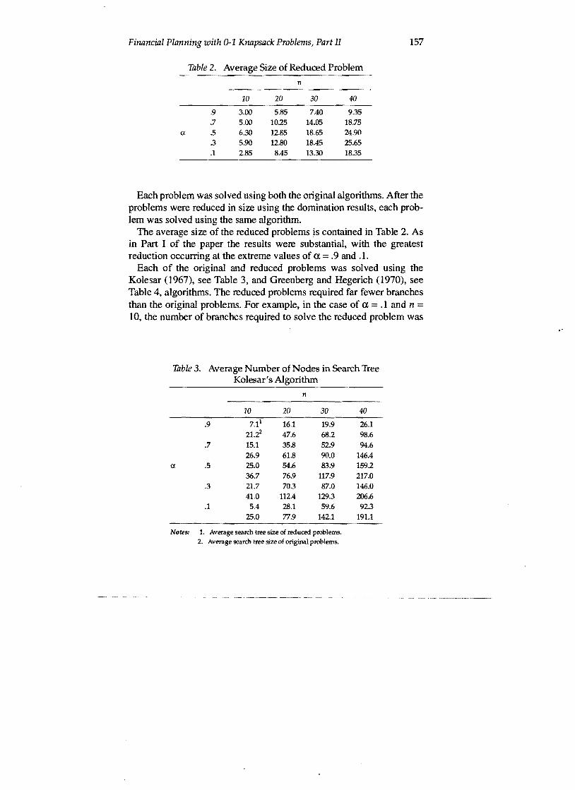
The average size of the reduced problems is contained in Table 2. As in Part I of the paper the results were substantial, with the greatest reduction occurring at the extreme values of a =.9 and .1.

Each of the original and reduced problems was solved using the Kolesar (1967), see Table 3, and Greenberg and Hegerich (1970), see Table 4, algorithms. The reduced problems required far fewer branches than the original problems. For example, in the case of a =.1 and n = 10, the number of branches required to solve the reduced problem was

Table 3. Average Number of Nodes in Search Tree Kolesar's Algorithm

n

10 20 30 40

.9 16.1 19.9 26.1 21.22 47.6 68.2 98.6

.7 15.1 35.8 52.9 94.6 26.9 61.8 90.0 146.4

a .5 25.0 54.6 83.9 159.2 36.7 76.9 117.9 217.0

.3 21.7 70.3 87.0 146.0 41.0 112.4 129.3 206.6

.1 5.4 28.1 59.6 92.3 25.0 77.9 142.1 191.1

Notes: 1. Average search tree size of reduced problems. 2. Average search tree size of original problems.


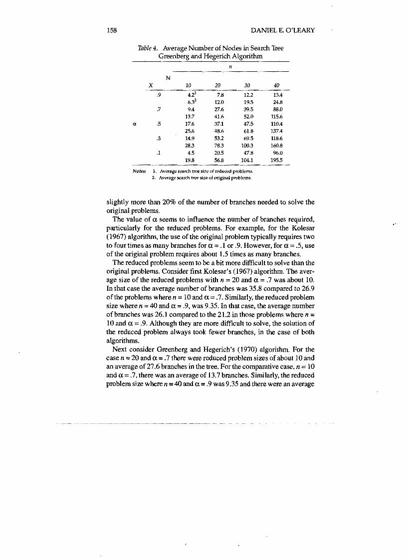
Table 4. Average Number of Nodes in Search Tree Greenberg and Hegerich Algorithm

n

N X 10 20 30 40

.9 7.8 12.2 13.4 6.32 12.0 19.5 24.8

.7 9.4 27.6 39.5 88.0 13.7 41.6 52.0 115.6

a .5 17.6 37.1 47.5 110.4 25.6 48.6 61.8 137.4

.3 14.9 53.2 69.5 118.6 28.3 78.3 100.3 160.8

.1 4.5 20.5 47.8 96.0 19.8 56.8 104.1 195.5


slightly more than 20% of the number of branches needed to solve the original problems.

The value of a seems to influence the number of branches required. particularly for the reduced problems. For example, for the Kolesar (1967) algorithm. the use of the original problem typically requires two to four times as many branches for a = .1 or .9. However, for a = .5, use of the original problem requires about 1.5 times as many branches.

The reduced problems seem to be a bit more difficult to solve than the original problems. Consider first Kolesar's (1967) algorithm. The average size of the reduced problems with n =20 and a =.7 was about 10. In that case the average number of branches was 35.8 compared to 26.9 ofthe problems where n = 10 and a. = .7. Similarly, the reduced problem size where n = 40 and a = .9, was 9.35. In that case, the average number of branches was 26.1 compared to the 21.2 in those problems where n = 10 and a =.9. Although they are more difficult to solve, the solution of the reduced problem always took fewer branches, in the case of both algorithms.

Next consider Greenberg and Hegerich's (1970) algorithm. For the case n = 20 and a. =.7 there were reduced problem sizes of about 10 and an average of 27.6 branches in the tree. For the comparative case, n =10 and a. =.7, there was an average of 13.7 branches. Similarly, the reduced problem size where n =40 and a. =.9 was 9.35 and there were an average

"

159 Finandal Planning with 0-1 Knapsack Problems, Part II

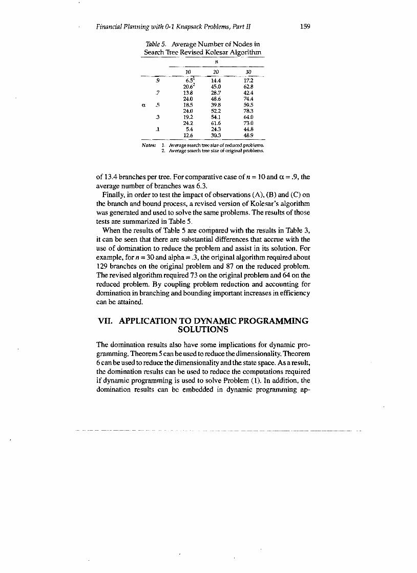
Table 5. Average Number of Nodes in Search Tree Revised Kolesar Alg~rithm

n

10 20 30

.9 6.51 14.4 17.2 20.62 45.0 62.8

.7 13.8 28.7 42.4 24.0 48.6 74.4

(l .5 18.5 39.8 59.5 24.0 52.2 78.3

.3 19.2 54.1 64.0 24.2 61.6 73.0

.1 5.4 24.3 44.8 12.6 30.3 48.9


of 13.4 branches per tree. For comparative case of n =10 and a =.9, the average number of branches was 6.3.

Finally, in order to test the impact of observations (A), (B) and (e) on the branch and bound process, a revised version of Kolesar's algorithm was generated and used to solve the same problems. The results of those tests are summarized in Table 5.

When the results of Table 5 are compared with the results in Table 3, it can be seen that there are substantial differences that accrue with the use of domination to reduce the problem and assist in its solution. For example, for n =30 and alpha =.3, the original algorithm required about 129 branches on the original problem and 87 on the reduced problem. The revised algorithm required 73 on the original problem and 64 on the reduced problem. By coupling problem reduction and accounting for domination in branching and bounding important increases in efficiency can be attained.

VII. APPLICATION TO DYNAMIC PROGRAMMING SOLUTIONS

The domination results also have some implications for dynamic programming. Theorem 5 can be used to reduce the dimensionality. Theorem 6 can be used to reduce the dimensionality and the state space. As a result, the domination results can be used to reduce the computations required if dynamic programming is used to solve Problem (1). In addition, the domination results can be embedded in dynamic programming ap

160

proaches. This section develops those results and illustrates them in the example.

A. Impact of Domination Results

Let.fi(y) be the optimal solution to

.fi(y) == max 'L crj j=J

Xj == 0 or 1,

where fo(Y) = 0 for all y :S; b (in the reduced problemfo(y) =1:j E i c j and y :S; b - 1:jEl a j • Theorems 5 and 8 can be restated to account for the structure of dynamic programming.

TheoremS'. Xi =0 in some optimal solution for y < ai + 'L aj •

Theorem 8', For ally;

y<a j +'Laj je Yj

in some optimal solution to Problem (1'). A number of recursions are available for finding h.(y) (e.g., Weingart

ner and Ness, 1967 and Morin and Marsten, 1974). Each of those recursions (and others) can be structured to account for Theorems 5' and 8'.

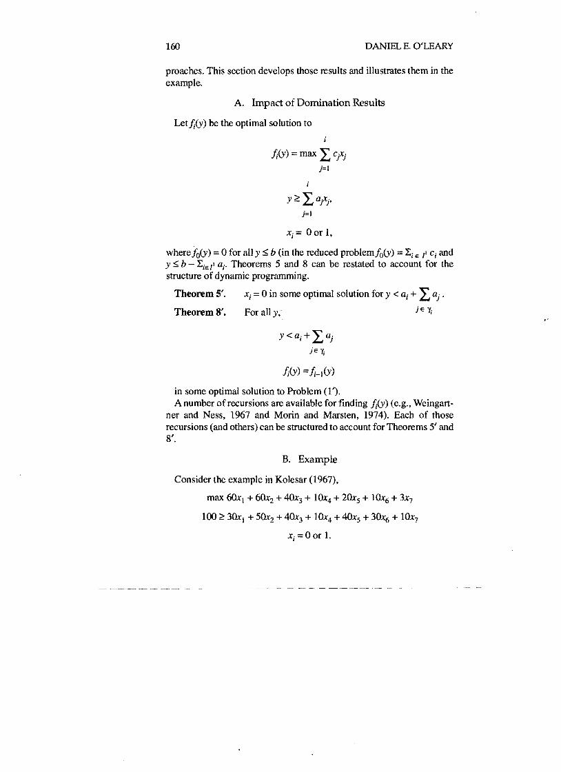
B. Example

Consider the example in Kolesar (1967),

max 60xl + 60x2 + 40x3 + IOx4 + 20xs + lOx6 + 3X7

100;;::: 30xI + 50x2 + 40x3 + lOx4 + 40xs + 30x6 + lOx7

Xj = 0 or 1.


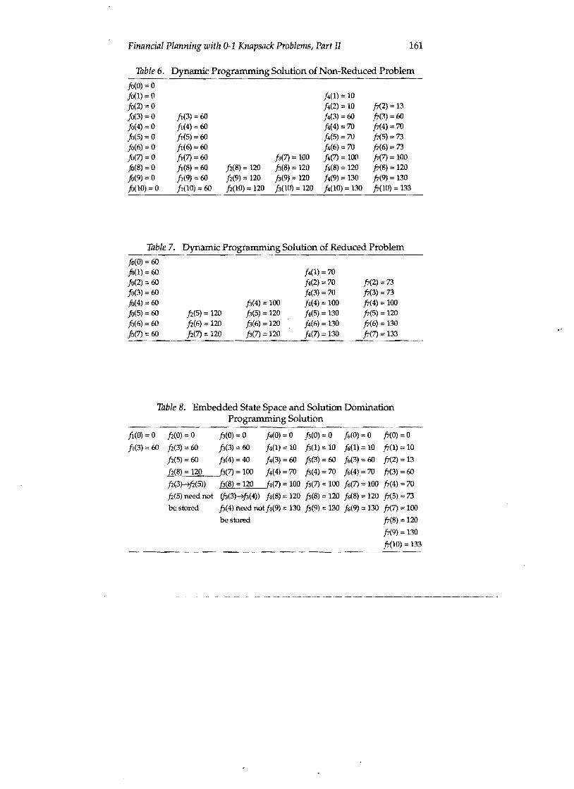
Table 6. Dynamic Programming Solution of Non-Reduced Problem

10(0) = 0 10(1) = 0 14(1) == 10 10(2) =0 /4(2) =10 ft(2) = 13

10(3) = 0 /1(3) == 60 14(3) == 60 ft(3) = 60

10(4) = 0 /1(4) '" 60 14(4) =70 ft(4) =70 fo(5) =0 11(5) '" 60 14(5) =70 ft(5) = 73

10(6) 0 ft(6) 60 14(6) '" 70 ft(6);: 73

10(7) == 0 /1(7) = 60 /3(7) =100 /4(7) =100 ft(7) =100 fo(8) == 0 ft(8);: 60 /2(8) == 120 /3(8) =120 14(8) =120 ft(8) == 120

fo(9) '" 0 /1(9) 60 /2(9) 120 13(9) 120 14(9) 130 ft(9) = 130

fo(lO) = 0 ft(10) = 60 12(10) =120 13(10) == 120 14(10) =130 ft(10) =133

Table 7. Dynamic Programming Solution of Reduced Problem

10(0) = 60

fo(l) =60 /4(1) = 70

/0(2) =60 /4(2) = 70 ft(2) == 73

10(3) '" 60 14(3) '" 70 ft(3) == 73

10(4) 60 /3(4) == 100 /4(4) == 100 ft(4) == 100

10(5) '" 60 12(5) = 120 /3(5) = 120 /4(5);: 130 ft(5) = 120

10(6) == 60 /2(6) = 120 /3(6) = 120 14(6) = 130 ft(6) =130 " fo(7) == 60 /2(7) == 120 /3(7) = 120 14(7) 130 ft(7) == 133

~---~-~

Table 8. Embedded State Space and Solution Domination Programming Solution

/1(0) == 0 /2(0) == 0 /3(0) == 0 14(0) = 0 15(0) == 0 16(0) =0 ft(0) =0

11(3) = 60 12(3) = 60 /3(3) == 60 14(1) =10 /5(1) =10 16(1) =10 ft(l) == 10

/2(5) = 60 13(4) =40 14(3) = 60 js(3) =60 16(3) == 60 ft(2) 13

h(8) =120 f3(7) 100 14(4) == 70 fs(4) == 70 16(4) == 70 ft(3) == 60

/2(3)-7/2(5» 13(8) == 120 f4(7) == 100 15(7) == 100 /6(7) =100 ft(4) == 70

12(5) need not (t3(3)~/3(4» 14(8) 120 15(8) == 120 16(8) 120 ft(5) == 73

be stored /3(4) need not14(9) == 130 15(9) '" 130 16(9) =130 ft(7) == 100

be stored ft(8) == 120

ft(9) == 130

ft(10) == 133


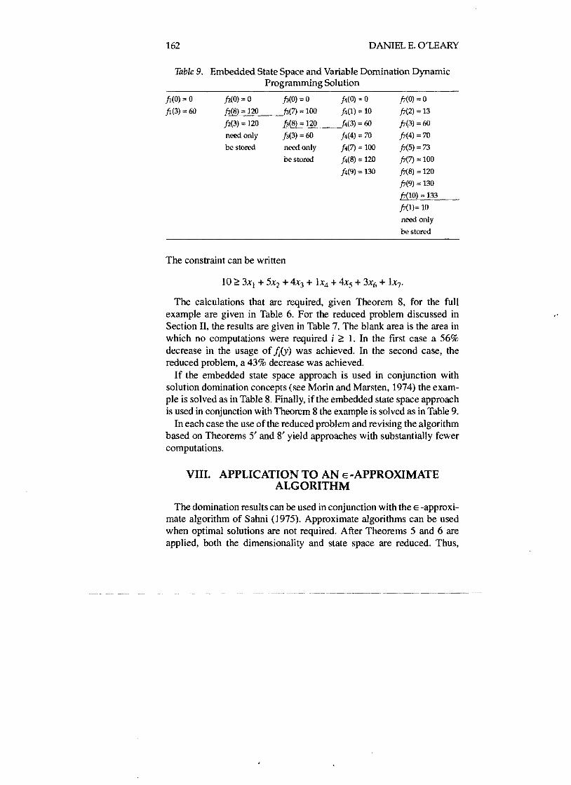
Table 9. Embedded State Space and Variable Domination Dynamic Programming Solution

fl(O) == 0 /2(0) = 0 ft(O) = 0 /4(0) = 0 ft(O) =0

fl(3) = 60 .L!;f2.>;;:(8L) =_1:;;;2:::..0_--,f3(7) = 100 f4(1) '" 10 ft(2) = 13

f2(3) =120 f3(8) = 120 f4(3) = 60 ft(3) =60

need only ft(3) = 60 f4(4) = 70 ft(4) '" 70

be stored need only f4(7) =100 ft(5) =73

be stored f4(8) = 120 ft(7) = 100

f4(9) =130 ft(8) =120

ft(9) =130

(7(10) = 133

ft(I)= 10

need only

be stored

The constraint can be written

10 ~ 3Xl + 5X2 + 4X3 + lx4 + 4xS + 3X6 + 1x7'

The calculations that are required, given Theorem 8, for the fun example are given in Table 6. For the reduced problem discussed in " Section II, the results are given in Table 7. The blank area is the area in which no computations were required i ~ 1. In the flTst case a 56% decrease in the usage of ,h(y) was achieved. In the second case, the reduced problem, a 43% decrease was achieved.

If the embedded state space approach is used in conjunction with solution domination concepts (see Morin and Marsten. 1974) the example is solved as in Table 8, Finally. if the embedded state space approach is used in conjunction with Theorem 8 the example is solved as in Table 9.

In each case the use ofthe reduced problem and revising the algorithm based on Theorems 5' and 8' yield approaches with substantially fewer computations,

VIII. APPLICATION TO AN E -APPROXIMATE ALGORITHM

The domination results can be used in conjunction with the E -approximate algorithm of Sahni (l975). Approximate algorithms can be used when optimal solutions are not required. After Theorems 5 and 6 are applied. both the dimensionality and state space are reduced. Thus,

163 Financial Planning with ()"'1 Knapsack Problems, Part II

Sahni's (1975) algorithm should be used on the reduced problem of Theorem 7. In addition, that algorithm can be altered to take into account the domination relationships.

C. Background: E -Approximate Algorithm

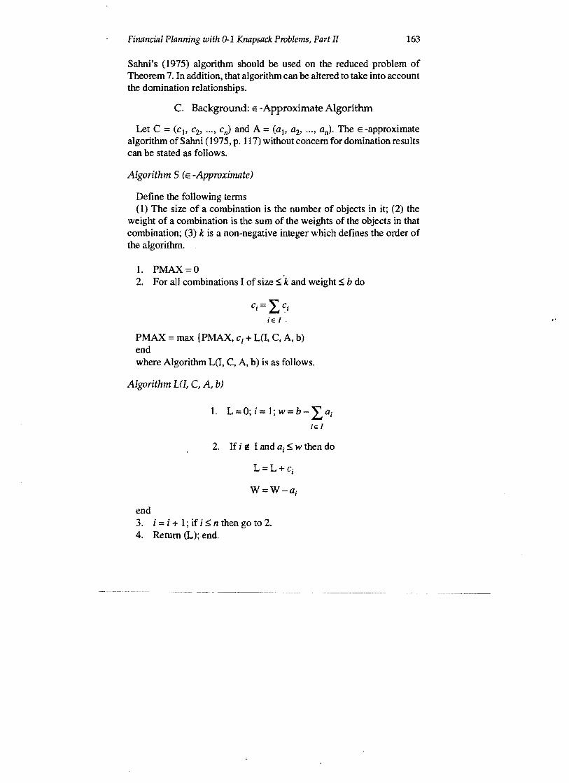
Let C = (c), cz, ... , cn) and A =(a), Oz, ... , an)' The E -approximate algorithm of Sahni (1975, p. 117) without concern for domination results can be stated as follows.

Algorithm S (E -Approximate)

Define the following terms (1) The size of a combination is the number of objects in it; (2) the

weight of a combination is the sum of the weights of the objects in that combination; (3) k is a non-negative integer which defines the order of the algorithm.

1. PMAX=O 2. For all combinations I of size ~ k and weight ~ b do

PMAX = max {PMAX, Cl + L(I, C, A, b) end where Algorithm L(I, C, A, b) is as follows.

Algorithm L([, C, A, b)

1. L = 0; i =1; w =b - L aj je I

2. If j re I and aj ~ w then do

W=W-aj

end 3. j = i + 1; if i ~ n then go to 2. 4. Return (L); end.


D. Accounting for Domination Results

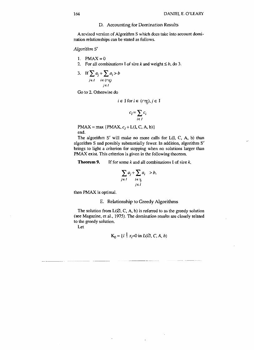
A revised version of Algorithm S which does take into account domination relationships can be stated as follows.

Algorithm S'

1. PMAX=O 2. For all combinations I of size k and weight ~ b, do 3.

3. If:Laj+ :Lai>b jE I iE (II'Y)

jE I

Go to 2. Otherwise do

i E Ifori E (nYj), j E I

PMAX =max {PMAX, C1+ L(I, C, A, b)} end. The algorithm S' will make no more calls for L(I, C, A, b) than

algorithm S and possibly substantially fewer. In addition, algorithm S' brings to light a criterion for stopping when no solutions larger than PMAX exist. This criterion is given in the following theorem.

Theorem 9. If for some k and all combinations I of size k,

:Laj+ :Laj >b, jE I iE 'Yj

jE I

then PMAX is optimal.

E. Relationship to Greedy Algorithms

The solution from L(0, C, A, b) is referred to as the greedy solution (see Magazine, et al., 1975). The domination results are closely related to the greedy solution.

Let

Ko ={i I x,=O in L(0, C, A, b)


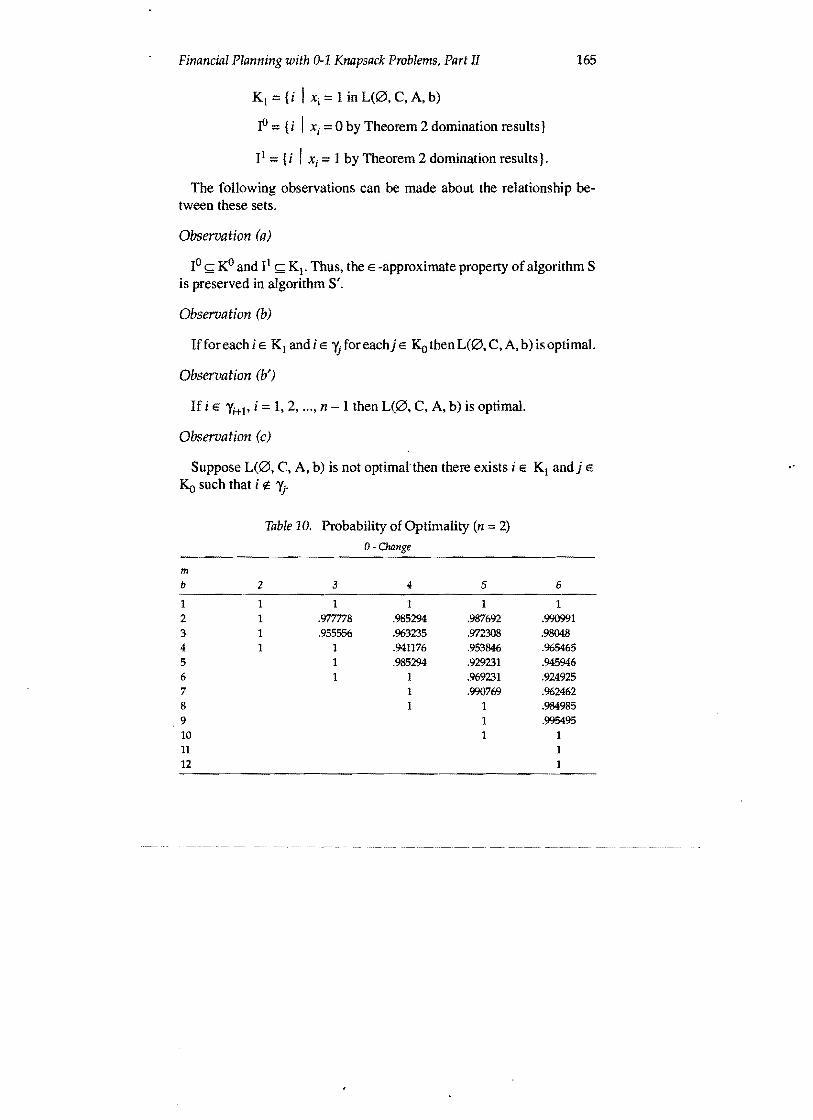
KI ={i I xi =1 in L(0, C, A, b)

fl = {i I xi = 0 by Theorem 2 domination results}

II = {i I xi = 1 by Theorem 2 domination results}.

The following observations can be made about the relationship between these sets.

Observation (a)

1°!;; KO and II!;; K1• Thus, the E -approximate property of algorithm S is preserved in algorithm S'.

Observation (b)

Iffor each i E Kl and; E ~foreachj E KothenL(0, C, A, b) is optimal.

Observation (b')

If i E Yi+l' i = 1,2, ... , n - 1 then L(0, C, A, b) is optimal.

Observation (c)

Suppose L(0, C, A, b) is not optimalthen there exists i E Kl andj E

Ko such that i e ~.

Table 10. Probability of Optimality (n ::: 2)

O-Change

m b 2 3 4 5 6

1 1 1 1 1 1 2 1 .977778 .985294 .987692 .990991 3 1 .955556 .963235 .972308 .98048 4 1 1 .941176 .953846 .965465 5 1 .985294 .929231 .945946 6 1 1 .969231 .924925 7 1 .990769 .962462 8 1 1 .984985 9 1 .995495 10 1 1 11 1 12 1

"


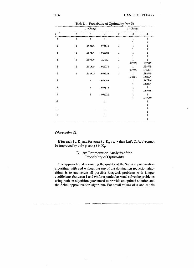
Table 11. (n =3)

a-Change 1 Change

b m 2 3 4 2 3 4

1 1 1 1 1 1 1 1 1

2 1 .963636 .971814 1 1 1 1 1

3 1 .957576 .942402 1 1 1 1 1

4 1 .957576 .92402 1 1 1 .993939 .997549

5 1 .981818 .946078 1 1 .998775 .993939 .996324

6 1 .981818 .958333 1 1 .998775 .987879 .988971

7 1 .974265 1 .997549 1 .988971

8 1 .981618 1 1 1 .987745

9 1 .996324 1 1 1 .997549

10 1 1 1

11 1 1 0'

1 12 1 1

1

Observation (d)

Iffor each i E Kl and for some j E Ko. i E "f; then L(0. C, A, b) cannot be improved by only placingj in K1•

D. An Enumeration Analysis of the Probability of Optimality

One approach to determining the quality of the Salmi approximation algorithm, with and without the use of the domination reduction algorithm, is to enumerate all possible knapsack problems with integer coefficients (between 1 and m) for a particular n and solve the problems using both an algorithm guaranteed to provide an optimal solution and the Sahni approximation algorithm. For small values of nand m this

167 Financial Planning with 0-1 Knapsack Problems, Part II

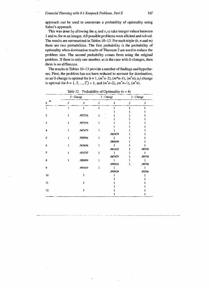
approach can be used to enumerate a probability of optimality using Sahni's approach.

This was done by allowing the a j and ci to take integer values between 1 and m, for m an integer. AU possible problems were elicited and solved. The results are summarized in Tables 10-13. For each triple (b, nand m) there are two probabilities. The ftrst probability is the probability of optimality when domination results of Theorem 2 are used to reduce the problem size. The second probability comes from using the original problem. If there is only one number, as is the case with O-changes, then there is no difference.

The results in Tables 10-13 provide a number of ftndings and hypotheses. First, the problem has not been reduced to account for domination, so an O-change is optimal for b = I, (m*n-2), (m*n-l), (m*n); aj-change is optimal for b = 1,2, ...• 2*j + 1, and (m*n-2). (m*n-l), (m*n).

Table 12. Probability of Optimality (n 4)

0- Change 1 Change 2 -Change m

b 2 3 2 3 2 3

1 1 1 1 1 1 1

1 1 1 2 1 .957576 1 1 1 1

1 1 1 3 1 .957576 1 1 1 1

1 1 1 4 1 .947475 1 1 1 1

.987879 1 1 5 1 .959596 1 1 1 1

.989899 1 1 6 1 .963636 1 1 1 1

.981818 1 .99798

7 1 .973737 1 1 1 1 .987879 1 .99798

8 1 .989899 1 1 1 1 .993939 1 .99798

9 .991919 1 1 1

.993939 .99596 10 1 1 1

1 1 11 1 1 1

1 1

12 1 1 1 1 1


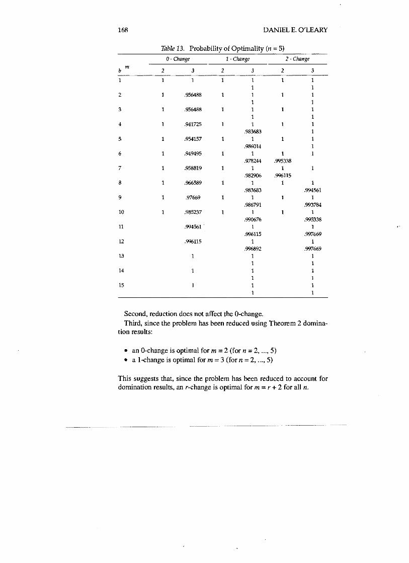
Table 13. Probability of Optimality (n = 5)

0 Change 1 Change 2 Change

mb 2 3 2 3 2 3

1 1 1 1 1 1 1 1 1

2 1 .956488 1 1 1 1 1 1

3 1 .956488 1 1 1 1 1 1

4 1 .941725 1 1 1 1 .983683 1

5 1 .954157 1 1 1 1 .986014 1

6 1 .949495 1 1 1 1 .978244 .995338

7 1 .958819 1 1 1 1 .982906 .996115

8 1 .966589 1 1 1 1 .983683 .994561

9 1 .97669 1 1 1 1 .986791 .993784

10 1 .985237 1 1 1 1 .990676 .995338

11 .994561 ' 1 1 " .996115 .997669

12 .996115 1 1 .996892 .997669

13 1 1 1 1 1

14 1 1 1 1 1

15 1 1 1 1 1

Second, reduction does not affect the O-change. Third, since the problem has been reduced using Theorem 2 domina

tion results:

• an O-change is optimal for m =2 (for n =2, ... , 5) • a I-change is optimal for m =3 (for n =2, ... , 5)

This suggests that, since the problem has been reduced to account for domination results, an r-change is optimal for m =r + 2 for alI n.


Fourth, since the problem has been reduced to account for domination results, a1'-change is optimal for l' =1, ... , 2*1' + 1.

IX. SUMMARY AND EXTENSIONS

Part I of this paper developed the notions ofdomination in 0-1 knapsack problems. Part II of this paper has used the notions of domination in two distinct ways. First, it studied the impact of reducing the problem size. Second, key notions of domination for 0-1 knapsack problems were embedded in different algorithms and used to improve the speed with which a solution could be found.

This pap€r could be extended in a number ofdifferent ways. First, the domination results can be extended to other types of solution processes. The branch and bound algorithms and dynamic programming approaches provided here were foriUustration purposes. Second, the results could be expanded to other problem types. For example, results could be developed for the bounded variable knapsack problem (e.g., Bruckner et al., 1975) and the multi-dimensional knapsack problems (e.g., Weingartner and Ness, 1967).

REFERENCES

Greenberg, H., and R. L. Hegerich. "A Branch and Search Algorithm for the Knapsack Problem," Management Science, Vol. 16, No.5 (1970).

Kolesar, P., "A Branch and Bound Algorithm for the Knapsack Problem," Management Science, Vol. 13, No.9 (1967).

Magazine, M. J., G. L. Nemhauser, , and L. E. Trotter, "When the Greedy Solution Solves a Class of Knapsack Problems," Operations Research, Vol. 23, No.2 (1975).

Morin, T., and R. E. Marsten, "Branch and Bound Strategies for Dynamic Programming," September 1974, Discussion Paper 106, Center for Mathematical Studies in Economics and Management Science, Northwestern University.

Sahni, S., "Approximate Algorithms for the 011 Knapsack Problem," Journal 0/ the Association o/Computing Machinery, Vol. 22, No. I (1975).

Weingartner, H. M., and D. N. Ness, "Methods of Solutions of the Multidimensional 011 Knapsack Problem," Operations Research, Vol. 15, No.1 (1967).

Weingartner, H. M., Mathematical Programming and the Analysis o/Capital Budgeting Problems. Englewood Cliffs, NJ, Prentice-Hall, 1962.

"

Documents

FINANCIAL PLANNING WITH 0-1 KNAPSACK PROBLEMS, … · A number of branch and bound algorithms have been presented for the solution ofthe 0-1 knapsack problem. Perhaps the fIrst branch