Embed Size (px)
Citation preview

Financial Performance Analysis of Banks:
Empirical Analysis with evidence from the
US Banking Sector
Anastasios Chatsios
SCHOOL OF ECONOMICS, BUSINESS ADMINISTRATION & LEGAL STUDIES
A thesis submitted for the degree of
Master of Science (MSc) in Banking & Finance
October 2017
Thessaloniki - Greece


[i]
PREFACE
Student Name: Chatsios Anastasios SID: 1103150003 Supervisor: Dr. Archontakis & Dr. Grose
I hereby declare that the work submitted is mine and that where I have made use of another’s
work, I have attributed the source(s) according to the Regulations set in the Student’s
Handbook.
October 2017 Thessaloniki - Greece
Anastasios Chatsios
Date: October 19, 2017

[ii]

[iii]
ABSTRACT
This thesis reports significant new findings on banking profitability by relating the internal
factors, the external factors with time dummy variables as control for financial crisis in the
test period. By employing a balanced panel data of 169 US banking institutions for the
timespan of fourteen years (2003-2016) and by creating two extra sub-samples, namely the
pre-crises (2003-2007) and post-crises (2008-2016), tries to investigate further into the bank
profitability determinants and how these determinants have been altered due to the financial
crises of 2008. More specifically, this analysis utilizes the most significant internal and
external factors of determinants, namely the risk management, the capital management, the
size of the bank, the expenses management and macroeconomic factors such as the gross
domestic product per capital growth, the long-term interest rates and the rate of inflation.
No previous study has investigated all these factors combined as determinants for the specific
period and there is no recent evidence of the financial crises effects on the determinants of
bank performance during this time span. Findings of the analysis indicate that he expected
relationships are confirmed except the effect of the interest rates that produced an opposing
to the expected result. Most of the factors seem to have a significant effect on bank
performance and since the internal factors are the ones that are more easy to be managed
some policy recommendations are being cited upon the results of this research. Finally, as it
was expected, some differences are being observed into what determines the profitability
after the burst of the 2008 financial crises. The determinants and especially the internal
factors seem to have a higher impact on bank performance and that is why the results suggest
that the bank performance is lower in the post-crises period.
Keywords: Bank Performance, Internal Factors, External Factors, Financial Crises, US Banking System.

[iv]

[v]
ACKNOWLEDGEMENTS
At this point, I would like to thank all the people who supported me during my MSc studies at
International Hellenic University.
I am really grateful to all the academic staff of the MSc in Banking and Finance, who provided
me with all the necessary knowledge and tools in order to complete my studies.
Especially, I am thankful to my dissertation supervisor Dr. Grose for his valuable guidance and
suggestions during the composition of this thesis and during my studies.
October 2017 Thessaloniki - Greece
Chatsios Anastasios
Date: October 19, 2017

[vi]

[vii]
Table of Contents PREFACE .................................................................................................................................................. i
ABSTRACT............................................................................................................................................... iii
ACKNOWLEDGEMENTS ........................................................................................................................... v
1. INTRODUCTION .............................................................................................................................. 1
2. THEORETICAL FRAMEWORK .......................................................................................................... 5
2.1. Literature Review .....................................................................................................................5
2.2. Bank Performance Determinants ......................................................................................... 10
2.2.1. Internal Factors ............................................................................................................ 11
2.2.2. External Factors ............................................................................................................ 12
2.3. Financial Crises and Bank Performance ................................................................................ 14
3. RESEARCH DESIGN ....................................................................................................................... 17
3.1. Research Methodology ......................................................................................................... 17
3.2. Data Collection and Sampling ............................................................................................... 18
3.3. Measurement and Selection of Variables ............................................................................. 18
3.3.1. Explained Variable ........................................................................................................ 19
3.3.2. Independent Variables ................................................................................................. 19
3.4. Specification of the Model .................................................................................................... 21
4. EMPIRICAL RESULTS AND DISCUSSION ....................................................................................... 23
4.1. Descriptive Statistics ............................................................................................................. 23
4.2. Correlations........................................................................................................................... 26
4.3. Regression Analysis ............................................................................................................... 28
4.4. Discussion of the Results ...................................................................................................... 32
4.4.1. Comparison with Prior Findings ................................................................................... 32
4.4.2. Policy Recommendations ............................................................................................. 33
5. CONCLUDING REMARKS .............................................................................................................. 35
5.1. Research Conclusions ........................................................................................................... 35
5.2. Research Limitations ............................................................................................................. 36
5.3. Suggestions for Future Research .......................................................................................... 36
REFERENCES ......................................................................................................................................... 37
APPENDIX ............................................................................................................................................. 41

[viii]
List of Tables and Figures Table 1: Number of Banks for each Type in the Sample ...................................................................... 18
Table 2: Expected Relationship of each Group of Variables ................................................................ 20
Table 3: Descriptive Statistics for the Pre-Crises Sample (2003-2007) ................................................ 23
Table 4: Descriptive Statistics for the Post-Crises Sample (2008-2016) .............................................. 24
Table 5: Descriptive Statistics for the Total Sample (2003-2016) ........................................................ 25
Table 6: Correlation Coefficients for the Pre-Crises Sample (2003-2007) ........................................... 26
Table 7: Correlation Coefficients for the Post-Crises Sample (2008-2016) ......................................... 27
Table 8: Correlation Coefficient for the Full Sample (2003-2016) ....................................................... 27
Table 9: Regression Analysis Models for the Pre and Post-Crises Samples ......................................... 28
Table 10: Regression Analysis Model for the Full Sample Period ........................................................ 30
Table 11: Comparison of the Research Outcome ................................................................................ 32
Table 12: Regression Analysis Output for Pre-crises and Post-crises Samples .................................... 41
Table 13: Redundant Fixed Effects Test for Pre-crises and Post-crises Samples ................................. 41
Table 14: Regression Analysis Output for Full Sample. No effects, Fixed Effects & Random Effects .. 42
Table 15: Redundant Fixed Effects Test and Random Effects Hausman Test ...................................... 43

[1]
1. INTRODUCTION During the years and especially the last decade, we can see that the financial sector of an
economy has an increasingly important role. More specifically, we can see that the most
significant matter that investors and academics deal with is the banking systems of each
country and their financial performance. That can be explained to the possible remarkable
impact that a banking system may has on the economic growth of a country. As a result, the
profitability of a banking institution is crucial for the stability of the financial sector and
consequently for the stability of the country’s stability that operates in.
In addition, the effects of a malfunctioning financial system could be affecting the financial
sectors of other countries too, making the so-called global financial crisis we are facing the last
decade. The trigger for the financial distress that E.U. countries face the last years, starting
from Iceland and spreading mainly in the Southern Europe, could be have its roots to the
policies applied in the U.S. banking system. Policies such as the facilitating access to loans and
the absence of sufficient capital for backing the obligations of banks and insurance companies
produced home ownership, which peaked in 2004. These practices resulted into the burst of
the bubble in late 2007 and beginning of 2008 and led to a large decline in real estate prices,
causing huge damage to financial institutions on a global scale (e.g. Lehman Brothers). Since
then, in all the banking systems we can see many alterations in the policies and strategies being
applied in order to increase their profitability and be more effective (Stiroh and Rumble, 2006).
As a result, we can see the importance of the financial institutions and especially the importance
of a large-scale one, such as the US banking system. Hence, there is a crying need for all the
parties concerned, to have a clear image, regarding the factors that determine the performance
of banks.
Prior literature has been abundant in the bank profitability determinants. The main groups of
determinants categorized into two groups, namely the internal and external factors. These are
described as the bank-specific, industry-specific and finally the macroeconomic factors.
However, there is no much evidence for the US banking sector concerning the effect of all the
groups together on bank profitability. Furthermore, most of the studies in literature, on bank
profitability use linear models for their estimations of the factors affecting the bank profitability
(Short, 1979; Bourke, 1989; Molyneux and Thornton, 1992; Goddard et al., 2004). By using a
simple linear model, some issues might not be dealt sufficiently. Firstly, many previous studies
use only bank and/or industry level variables as factors without accounting for the

[2]
macroeconomic environment. In addition, in many studies the econometric analysis used in the
research methodology is not sufficiently described, implying inconsistency in the whole
analysis.
This dissertation will be innovative in three ways. Firstly, will formulate a full model including
all the groups of factors affecting the bank profitability that it is scarce in the US prior literature.
Secondly, the use of pre-crises and post-crises bank-data will allow us to capture and report
the effect that the financial crises of 2008 had on the bank profitability determinants. Finally,
the updated dataset will provide us with new insights for the movement of the profitability
determinants the last years. More specifically, this thesis contributes to the literature by using
all the group of factors affecting the bank performance, namely the internal (bank-specific) and
external (macroeconomic) factors, for the recent years in order to capture the effect of the
financial crises. Examining the disclosed return on average equity figures for the years 2003-
2016 and in a special way of creating sub-samples (pre and post-crises), provides evidence to
the extent of what banks must consider as important in order to be more profitable.
The aim of this thesis is to empirically assess in a single equation framework the effects of the
factors that define profitability in US banking system, before and throughout the recent
economic crisis, as well as to offer new insights into the debate of which variables are the most
significant for measuring bank performance. More specifically, some possible determinants of
bank performance are being examined by using a dataset of US banks for the period 2003-
2016, by formulating an appropriate model. Furthermore, the second main aim of this thesis is
to determine the effect of the recent global financial crises on US bank performance. In order
to achieve that, the dataset is going to be separated into two sub-datasets, namely the pre-crises
and the post-crises, consisting of the periods 2003-2007 and 2008-2016 respectively. The
analysis followed in this thesis will be the panel data analysis, using a balanced panel for the
aforementioned time-period, in order to obtain the effect of the determinants and two more
panel data analyses using the sub-periods datasets in order to obtain the financial crises effect.
The analysis is incorporating in the model the two major groups of variables, namely the
internal and external factors of bank profitability. The internal factors consist of the bank’s
size, capital adequacy, expenses and risk management. The external factors are categorized in
the industry related factors (industry concentration) and the macroeconomic factors (long-term
interest rates, inflation rate and gross domestic product per capital). It worth to be mentioned
that due to lack of available data the industry related factors were not incorporated in the
analysis.

[3]
In line with the prior literature and the predicted outcome of this analysis the internal factors
are mainly affect the bank profitability in a positive way. In the notion that the less the risk that
the bank faces the higher the performance will be. In addition, the bigger the bank is, in capital
and in size, the higher the performance would be. Furthermore, the macroeconomic
environment is expected to increase the bank performance when it is favorable for the bank.
Meaning that the higher the economic growth is, the higher the bank performance would be.
The findings of this analysis, is mostly in line with the expected outcome and prior literature
mentioned in this paragraph, except some slight divergences. The reasons behind the results
opposed to prior literature are being analyzed in the final parts of this thesis. An interesting
finding of this empirical analysis is the degree that the bank performance in US has been
affected by the financial crises. The results suggest that from 2008 until recently (2016) the
bank performance has been severely damaged.
The thesis following this introduction consists of five more chapters. Chapter 2 is the
theoretical framework consisting of a thorough literature review on the subject of the bank
performance determinants and the alterations made to them during the financial crises of 2008.
Chapter 3 presents all the necessary details concerning the research performed. Chapter 4
illustrates the empirical analysis’ findings and discusses the possible implications and
recommendations of those findings. Finally, the last Chapter 5 provides some concluding
remarks and suggestions for future researches.

[4]

[5]
2. THEORETICAL FRAMEWORK This chapter discusses the main determinants of bank profitability through the presentation of
the prior literature on bank performance. Furthermore, the literature regarding the financial
crisis effect on bank performance is presented. Finally, the determinants’ characteristics and
expected relationship is discussed in the final part of this chapter.
Financial performance of banks has been the center subject of many previous researches over
the years. In the literature, the financial performance is linked with the ideas of efficiency and
profitability of the bank and more specifically, is linked as a function of Return on Average
Equity (ROAE) and Return on Average Assets (ROAA). Most of the studies categorize the
factors as internal and external determinants of financial performance of banks. The internals
are the factors mainly driven by bank-specific factors, while the external are the factors driven
by the financial and legal framework of the banking sector. Thus, industry-specific factors are
included in the external factors category.
2.1. Literature Review The first researches in the bank profitability field, which tried to shed light into the
determinants of bank profitability, were performed by Short (1979) and Bourke (1989).
Specifically, the findings of Short (1979), suggested that a positive relationship exists between
the profitability and the market power. The results from the analysis of Bourke (1989),
suggested that profitability is positively related to liquidity, capital ratios and interest rates. All
the studies after those were based on the two first studies and can be separated into two
categories, those who performed a country analysis and those who performed several countries
analysis. In the first category belong Berger (1995), Athanasoglou et al. (2008), Kosmidou
(2008), Bennaceur and Goaied (2008), García-Herrero et al. (2009), Dietrich and Wanzenried
(2011), Alper and Anbar (2011) and Trujillo‐Ponce (2013) whose researches centered the
determinants of bank profitability of a single country. Concerning the second category, the
studies of Molyneux and Thornton (1992), Demirgüç-Kunt and Huizinga (1999), Abreu and
Mendes (2001), Staikouras and Wood (2004), Goddard et al. (2004), Athanasoglou et al.
(2006) and Pasiouras and Kosmidou (2007) centered their research on a cross-country level.
The first researches on bank profitability on a cross-country level were those of Bourke (1989)
and of Molyneux and Thornton (1992). Bourke (1989) utilized a dataset comprising of banks
from twelve countries, while Molyneux and Thornton (1992) used a dataset of eighteen
European countries. The results from these two researches are similar in terms of factors
affecting the banks’ profitability except the factors of liquidity and government ownership.

[6]
More specifically, concerning the internal factors both studies found a positive and statistically
significant relationship between bank profitability and expenses, signaling that the quality of
administration can affect the performance of banks. On the other hand, Bourke (1989) found
that liquidity risk is positively related with profitability of the bank, while Molyneux and
Thornton (1992) resulted on the opposite outcome. Concerning the external factors, both
studies found that there is a positive relationship between the bank concentration and bank
profitability. The different results derived in the government ownership, where Molyneux and
Thornton (1992) found a positive relationship with bank profitability, while Bourke (1989) a
negative relationship. The different results could be attributed to the differentiations in the
datasets used for the analysis.
Demirgüç-Kunt and Huizinga (1999) used a sample comprising of 80 countries’ bank-level
data for the years 1988-1995 to determine the bank profitability and interest margin factors. In
their research, they incorporated variables that have never been utilized in the past, such as the
financial structure, legal, ownership and tax factors. The results showed that capitalization and
bank profitability are positively related. In fact they cited that this is rational, considering that,
better-capitalized banks have higher equity and are less likely to diminish, due to their minor
need for external financing. In the same result recently concluded Laeven et al. (2016), who by
using an international dataset of countries, found a positive relationship between the capital
structure of the bank with its performance along with the rest of the determinant such as the
bank size and systemic risk.
Abreu and Mendes (2001) investigated the factors determining the bank performance regarding
Portugal, Germany, France and Spain. The outcomes show that a higher equity to assets ratio
leads to higher bank profitability and net interest margins. In addition, there is a positive
relationship between the loan to assets ratio and profits. Furthermore, the findings show a
positive reaction of net interest margins towards operating costs, but this does not apply to
profitability. In conclusion, inflation is consistent and the nominal effective exchange rate does
not affect profitability. In the same notion, the same results were produced by Djalikov and
Piesse (2016), who resulted in a positive relationship between he macro-economic factors and
bank profitability, yet an insignificant one.
Staikouras and Wood (2004) investigated on how internal and external factors affect bank
performance by using the entire European banking sector (thirteen banking markets) for a time
span of 1994-1998. The outcomes regarding the internal factors showed that there is positive

[7]
relationship between the equity to assets ratio and profitability and a negative relationship
between loan to assets ratio and bank profitability. Regarding the external factors, finding show
a negative impact from the volatility of interest rates and GDP growth, while a positive
correlation exists between the level of interest rates and bank profitability.
Goddard et al. (2004) used a sample comprising of France, Germany, Italy, Denmark, Span
and United Kingdom for the years from 1992 to 1998 in order to identify the determinants of
bank profitability. The results from the research indicate that bank profits and off-balance-sheet
size are positively interrelated, with respect to United Kingdom. However, this relationship is
neutral or even negative, concerning other investigated countries. Moreover, bank size and
ownership status do not correlate with its performance. A positive correlation has been found
between the capital adequacy ratio and profitability.
The subsequent year Kosmidou et al. (2005), used a dataset of 32 UK owned commercial banks
for the years 1995-2002, in order to investigate the effect of bank-specific, macroeconomic
factors in addition to the financial market structure on bank performance. The results depicted
that equity to assets ratio (capital strength) constitutes the most important factor determining
the bank profitability. Moreover, the outcomes revealed that cost-to-income ratio and bank size
are negatively correlated with bank performance. However, the findings about the effect of
liquidity and loan loss reserves on Return on Average Assets are controversial. Finally, the
external factors have a significant effect on bank performance only individually, as their total
explanatory contribution to the model is small.
Athanasoglou et al. (2006) investigated the impact of bank-specific, industry-related and
macroeconomic indicators on the performance of South Eastern European banking institutions.
The analysis was performed by using an unbalanced panel data of 7 countries for the years
1998-2002. The results showed that bank profitability is affected in the expected manner from
all the internal (bank-specific) factors except the liquidity risk that showed a negative
correlation yet an insignificant one. The explanation given for this result is that South Eastern
European banks, by keeping an illiquid position to avoid failures, do not have the resources to
achieve a liquidity level, similar to that of developed banking systems. One more important
result from the analysis is that structure-conduct-performance hypothesis holds, since the
influence of market concentration is positive. However, concerning the macroeconomic
factors, the outcomes are controversial, considering that inflation has a substantial impact on
[8]
bank profits, whereas bank profitability is not seriously influenced by the variations of real
GDP per capital.
Pasiouras and Kosmidou (2007) used a bank-level data for 15 European countries for the period
1995-2001, in order to determine the impact of bank-specific factors and total bank
environment on the bank’s profitability. In this study, new variables are incorporated such as
the stock market capitalization to GDP and total assets of deposit money to GDP. The research
results suggest that equity to assets and ROAA are positively associated, while cost to income
ratio and profitability are negatively associated. The two most important factors determining
the profitability of the banks were the equity to assets ratio and cost to income ratio, for the
domestic and foreign banks respectively. Furthermore, size and profitability are negatively
correlated for both domestic and foreign banks. To conclude, GDP growth and inflation have
both a significant effect on profitability but with contrary signs on domestic and foreign banks.
Bennaceur and Goaied (2008) investigated an analysis in order to define the determinants of
bank profitability by using a sample of Tunisian banks for the years 1980-2000. Their findings
suggest that great amounts of capital have a positive impact on profitability and net interest
margin. In addition, they found that there is a positive effect of bank loans with net interest
margin and a negative effect of bank size on profitability. Concerning the external factors, both
economic growth and inflation have no significant impact on profitability of Tunisian banks.
Finally, a positive effect of stock market development on bank profitability is suggested,
indicating a connection between stock market and bank growth.
Kosmidou (2008) used an unbalanced time series data of 23 Greek banks for the period 1990-
2002, in order to determine the factors of bank performance. The results showed a positive and
statistically significant relationship between bank performance and equity to assets ratio, as
and a negative and statistically significant correlation of bank performance and cost to income
ratio. Furthermore, ROAA and liquidity ratio are statistically significantly and negatively
correlated, in case where only bank-specific factors are included in the model. On the contrary,
a positive and statistically insignificant relation between ROAA and liquidity ratio is observed
when macroeconomic and financial structure factors are introduced into the model. Moreover,
size was found positively correlated with bank profitability in every case, but statistically
significant only when macroeconomic and financial structure factors are input in the model.
Regarding macroeconomics and financial structure, GDP growth has a significantly positive
effect on ROAA, in contrast with the significantly negative effect of inflation on ROAA.

[9]
Athanasoglou et al. (2008) investigated the impact of bank-specific, industry-related and
macroeconomic factors on bank performance. They used a dataset comprising of Greek banks
for the years 1985-2001. They found that the banking sector profitability is considerably
affected in the expected manner by all bank-specific factors, except size. Furthermore, a
continuation in bank profits is observed, signifying the possibility of not that large deviation
from perfect competition in market structure, whereas the structure-conduct-performance
hypothesis is not supported by the findings. As far as the industry-related determinants are
concerned, concentration and ownership do not affect significantly bank performance. Finally,
on the macroeconomic factors’ side, business cycle and inflation have an obvious effect on
bank profitability.
The low profitability of Chinese banks attracted the attention of Garcia-Herrero et al. (2009).
They performed an empirical analysis in order to study the determinants of that low
profitability, by using a sample of 87 Chinese banks for the years from 1997 to 2004. The
differentiation of this study is the incorporation of two new measures of bank profitability,
namely ROA and pre-provisions profits. The outcomes suggest that highly capitalized banks,
with a greater number of deposits and efficiency are more lucrative. During that period,
profitability in China appears to be enduring, due to the competition limits and the high degree
of state interference.
Goddard et al. (2010) investigated into the determinants and the persistence of bank
profitability by using banks from eight European countries for the period 1992-2007. The
analysis was performed by splitting the dataset into two sub-periods pre-euro establishment
(1992-1998) and post-euro establishment (1999-2007). The results suggested that profits do
not changed during the first sub-period, denoting that banks with excess profits this year are
more likely to make higher excess profits the following year. However, a decrease in
continuation of the second sub-period is observed. That could be attributed to the increased
competition that exists from 1999 onwards. The relationship between bank profitability and
non-interest income to total operating income is positive and statistically significant,
concerning the majority of estimations. This is an indication that banks with a higher
diversification are more lucrative. In addition, a negative relation between profitability and
capital ratio is observed, implying that better capitalized banks are less profitable, because of
their lower level of risk. Finally, the empirical evidence concerning the relationship between
profitability and market share is controversial, while it is found that profitability and
concentration are inversely correlated.

[10]
Finally, the most recent study on the factors affecting the bank profitability is that of Trujillo‐
Ponce (2013), who investigated into the major factors affecting the high profitability of Spanish
banks. The analysis was performed by using a sample of 89 banks for the period of 1999-2009.
The findings suggest that the large bank profits are related to a high proportion of loans in total
assets, a large rate of customer deposits, improved efficiency and low levels of doubtful assets.
Furthermore, it is found that more highly capitalized banks are capable of making higher
profits, only when ROA is considered as the indicator of profitability. Nevertheless, an increase
of equity to total assets ratio decreases the banks’ ROE, due to the reduction in leverage. As a
result, the high degree of Spanish banks’ capitalization over the examined period might have
enhanced their ROA, at the expense of their ROE. Moreover, efficiency is proved a significant
determinant of bank profits, whereas size and income diversification do not seem to have a
significant impact on the explanation of Spanish banks’ profitability, because of the absence
of economies or diseconomies of scale and scope. As far as external determinants are
concerned, the outcomes of the study indicate the significance of business cycle for banks’
profitability and verify that market concentration is positively related to the profits of the
Spanish banking sector. Finally, inflation and interest rates have a clear effect on bank
profitability as well.
2.2. Bank Performance Determinants Prior literature has divided the bank profitability determinants into two big categories, namely
the internal and external factors. The internal factors or otherwise bank-specific factors are
associated with the bank accounts (balance sheet, profit and loss accounts). On the other hand,
the external factors are associated with the reflection of the economy and the legal bank
environment that affect the operations and the structure of the institution. As it is already
analyzed in the previous parts of this thesis, the researches undertaken in order to determine
the effect of these factors on bank profitability. Thus, the proposed variables for each factor,
according to the nature and purpose of each study, are in abundance.
The researches performed concentrated on profitability analysis of either cross-country or
individual countries’ banking systems. These are the studies thoroughly presented in the
previous section and all of the above studies examine various combinations of internal and
external determinants of bank performance. The empirical results vary significantly, since the
data samples and environments differ. There exist, however, some common elements that allow
a further categorization of the determinants.
[11]
2.2.1. Internal Factors
The variables employed by the prior literature, as internal or bank-specific factors, usually are
the risk management, size, capital and expenses management.
The risk management actions in the banking sector are very important for each banking
institution and for the banking system as a whole. Poor asset quality and low levels of liquidity
are the two major causes of bank failures. During uncertainty, banks may decide to diversify
their portfolios and/or raise their liquid holdings in order to reduce their risk. In this respect,
risk can be categorized into liquidity and credit risk. Molyneux and Thornton (1992) and
Laeven et al. (2016), among others, find a negative and significant relationship between the
level of bank liquidity and profitability. On the other hand, Bourke (1989) reports that the effect
of credit risk on profitability appears clearly negative (Miller and Noulas, 1997; Poi et al.,
2017). That could be explained by the fact that when financial institutions are exposed to high-
risk loans, the accumulation of unpaid loans increases, implying that these loan losses have
produce lower returns to many commercial banks.
Size is introduced to account for existing economies or diseconomies of scale in the market.
Smirlock (1985) and DeYoung and Rice (2004) resulted in a positive and significant
relationship between size and bank profitability. Demirguc-Kunt and Huizinga (2000) suggest
that various financial, legal and other factors that affect bank profitability is closely linked to
firm size. Furthermore, as Short (1979) stated that size is closely related to the capital adequacy
of a bank since relatively large banks tend to raise less expensive capital and as a result appear
more profitable. In the same notion, Haslem (1968), Short (1979), Bourke (1989), Molyneux
and Thornton (1992) Bikker and Hu (2002), Goddard et al. (2001) and Laeven et al. (2016), all
link bank size to capital ratios, which they claim to be positively related to size, meaning that
as size increases, profitability rises. However, there are many researchers suggesting that little
cost saving can be achieved by increasing the size of a banking firm (Berger et al., 1987),
implying that eventually large banks may face scale inefficiencies.
Bank expenses are also a very important factor of profitability, closely related to the efficient
management. There is extensive prior literature on the idea that variables related to the
expenses should be included in the cost part of a standard microeconomic profit function. For
example, Bourke (1989) and Molyneux and Thornton (1992) find a positive relationship
between better-quality management and profitability. In line with these results are the outcome
of the analysis of Anarfi et al. (2016), who found a positive relationship between the two
variables.

[12]
2.2.2. External Factors
Concerning the external determinants of bank performance, it should be noted that we could
further distinguish between control variables that describe the macroeconomic environment,
such as interest rates, inflation and cyclical output, and variables that are associated with the
industry or market characteristics. The second refers to industry size, market concentration and
ownership status.
Industry-related Factors
A completely new trend about structural effects on bank profitability started with the
application of the Market-Power (MP) and the Efficient-Structure (ES) hypotheses. The MP
hypothesis, which is sometimes also referred to as the Structure-Conduct-Performance (SCP)
hypothesis, asserts that increased market power yields monopoly profits. A special case of the
MP hypothesis is the Relative-Market-Power (RMP) hypothesis, which suggests that only
firms with large market shares and well-differentiated products are able to exercise market
power and earn non-competitive profits (Berger, 1995). Likewise, the X-efficiency version of
the ES (ESX) hypothesis suggests that increased managerial and scale efficiency leads to
higher concentration and, hence, higher profits.
Studies, such as those by Smirlock (1985), Berger and Hannan (1989) and Berger (1995),
investigated the profit-structure relationship in banking, providing tests of the aforementioned
two hypotheses. To some extent the RMP hypothesis is verified, since there is evidence that
superior management and increased market share (especially in the case of small-to medium-
sized banks) raise profits. In contrast, weak evidence is found for the ESX hypothesis.
According to Berger (1995), managerial efficiency not only raises profits, but also may lead to
market share gains and, hence, increased concentration, so that the finding of a positive
relationship between concentration and profits may be a spurious result due to correlations with
other variables. Thus, controlling for the other factors, the role of concentration should be
negligible. Other researchers argue instead that increased concentration is not the result of
managerial efficiency, but rather reflects increasing deviations from competitive market
structures, which lead to monopolistic profits. Consequently, concentration should be
positively (and significantly) related to bank profitability. Bourke (1989), and Molyneux and
Thornton (1992), among others, support this view.
A rather interesting issue is whether the ownership status of a bank is related to its profitability.
However, little evidence is found to support the theory that privately owned institutions will
return relatively higher economic profits. Short (1979) is one of the few studies offering cross-

[13]
country evidence of a strong negative relationship between government ownership and bank
profitability. In their recent work, Barth et al. (2004) claim that government ownership of banks
is indeed negatively correlated with bank efficiency. In contrast, Bourke (1989) and Molyneux
and Thornton (1992) report that ownership status is irrelevant for explaining profitability.
Macroeconomic Factors
Lastly, the final group of profitability factors deals with macroeconomic control variables. The
variables normally used are the inflation rate, the long-term interest rate and/or the growth rate
of money supply. Revell (1979) investigates the relationship between bank profitability and
inflation and he states that the effect of inflation on bank profitability depends on whether
banks’ wages and other operating expenses increase at a faster rate than inflation. The question
is how mature an economy is so that future inflation can be accurately forecasted and thus
banks can accordingly manage their operating costs. In this notion, Perry (1992) argues that
the extent to which inflation affects bank profitability depends on whether inflation
expectations are correctly forecasted. An inflation rate fully anticipated by the bank’s
management implies that banks can appropriately adjust interest rates in order to increase their
revenues faster than their costs and thus acquire higher economic profits. Most studies (Bourke,
1989; Molyneux and Thornton, 1992) have shown a positive relationship between either
inflation or long-term interest rate and profitability.
Demirguc-Kunt and Huizinga (2000) and Bikker and Hu (2002) attempted to identify possible
cyclical movements in bank profitability or in other words the extent to which bank profits are
correlated with the business cycle. Their findings suggest that such correlation exists, although
the variables used were not the right measures of the business cycle. Demirguc-Kunt and
Huizinga (2000) used the annual growth rate of GDP and GNP per capita to identify such a
relationship, while Bikker and Hu (2002) used a number of macroeconomic variables (such as
GDP, unemployment rate and interest rate).
To conclude, the existing literature provides a rather comprehensive account of the effect of
internal and industry-specific determinants on bank performance, but the effect of the
macroeconomic environment is not investigated in detail. The time dimension of the panels
used in empirical studies is usually too small to capture the effect of control variables related
to the macroeconomic environment. Furthermore, sometimes there is an overlap between
variables in the sense that some of them proxy the same profitability determinant. Thus, studies
concerning the profitability analysis of the banking sector should address the above issues more
adequately, to provide a better insight into the factors affecting bank performance.

[14]
2.3. Financial Crises and Bank Performance The researches concerning the effect of the recent financial crisis on the determinants of bank
profitability are not in abundance.
Beltratti and Stulz (2009) studied the bank profitability determinants, using banks with large
stock returns at a worldwide level for the period of July 1st 2007 to December 31st 2008. Their
conclusion was that bank’s financial statement, regulatory framework and governance are
important for the comprehension of bank’s profitability for the period of crisis. The research
outcome suggested that banks with higher Tier I capital ratio and higher in number deposits
and loans, in addition to those that are under stricter monitoring, demonstrate higher
profitability for the period under investigation. However, banks that operate in countries with
stricter regulatory framework demonstrate worse profitability for the investigated period.
Xiao (2009) studied the performance of French banks and the financial support actions that the
government took during the period 2006-2008. The outcome of the research proved that despite
the fact that French banks are invulnerable to the financial crisis, they are critically resistant to
it. In fact the risks that banks faced was controlled through the diversification in financing,
geographical coverage and business activity overall. In addition, the preventive regulation, the
competent regulatory authorities and the strict supervision provided the banking system of
France an important tool to resist and recover from the crisis.
Cornett et al. (2010) investigated how the changes in internal corporate governance structures
in the banking sector affect the performance of U.S. banks, before and throughout the financial
crisis. The empirical results suggest that bank performance decreases during the crisis period,
as well as many aspects of corporate governance, such as board independence and executive
stock ownership. However, larger banks experience the biggest losses and deal with the biggest
changes in corporate governance. Furthermore, it is argued that the stock market returns of
2008 are strongly associated to corporate governance mechanisms, regarding large banks, but
not so much concerning smaller banks.
Dietrich and Wanzenried (2011) performed an empirical analysis, in order to investigate on the
influence of bank-specific, industry-related and macroeconomic determinants on the
profitability of 372 Swiss banks for period of 1999-2009. They divided the investigated period
into two sub-periods to elaborate on the effects of the financial crisis. The first sub-period
includes the pre- crisis (1999-2006), while the second sub-period involves the post-crisis period
(2007-2009). The research results indicate that operational efficiency is positively related to

[15]
bank profitability in both investigated sub-periods, while capitalization is significantly and
negatively related to bank profits, only during the crisis period. Furthermore, the growth of
loan volume above the average has a positive influence on bank profitability, whereas there is
a significantly inverse relationship between funding costs and ROAA, only during the pre-
crisis period. Moreover, banks with a higher proportion of interest income are less profitable
than banks with a more diversified total income, both before and during crisis. As far as
ownership structure is concerned, they concluded that government-owned banks make more
profits than private banks during the crisis, because they are characterized more safe. The study
also reveals the negative and statistically significant relation between bank profitability and
taxes in all cases, regarding the external factors.

[16]

[17]
3. RESEARCH DESIGN This particular chapter is a description of the research analysis performed for the empirical part
of this thesis. Firstly, the methodology of the research is analyzed. Then the data collection
process along with the sampling method is explained. Finally, the variables used as a proxy in
order to explain the aforementioned theory is cited, along with the final model used for the
analysis.
3.1. Research Methodology As it was mentioned in earlier section of this research, the main aim of this thesis is to
determine the factors affecting the financial performance of the banks and how the recent
financial crisis of 2008 affected the factors of financial performance. Hence, the research will
be divided into three parts. A whole sample analysis will be performed for the years 2003-2016
and two more samples will be created by splitting the whole sample into two sub-samples
namely the pre-crisis sample for the years 2003-2007, and the post-crisis sample concerning
the years 2008-2016. All the analyses will be performed by deploying the same model in order
to determine the factors affecting the financial performance of US banks.
The calculations performed with the use of EViews 7 and MS Excel. Each of the
aforementioned sub-samples and total sample is controlled for time, so it is firstly assessed
with only cross-sectional fixed effects regression. Following the aforementioned regression,
the Redundant Fixed Effects Likelihood Ratio Test is conducted, which suggests if it is better
to use a simple pooled estimation or a cross-sectional fixed effect model. In addition, the
Hausman test is conducted, in order to be decided whether the random effects model is better
for the analysis than the fixed effects model. Using the appropriate critical values, if the
probability obtained from the test is higher than the critical values that follow the chi-squared
distribution, the fixed effect is the appropriate model. Concerning this analysis and specifically
for the main sample and both sub-samples, cross-section fixed effect model is appropriate
according to the results of the Hausman test.
In addition, the heteroscedasticity presence in the residuals is also being checked. Thus, by
estimating the sample and sub-samples deploying the White cross-section coefficient
covariance method in the panel analysis in order to have robust model. Comparing the
Lagrange Multiplier (LM) coefficient, obtained from the Breusch-Pagan Test, with the critical
value of chi-squared, it does not indicate that heteroscedasticity in residuals is present.
[18]
3.2. Data Collection and Sampling The appropriate data needed was collected from three sources namely the BankScope
database, Bloomberg database and finally from the official annual reports of certain US banks
that are provided through their websites. The bank dataset was initially comprised from 1,360
US financial institutions with NAICS code 5221 and have been underwent a quality test. The
criteria of the data availability from 2003 to 2016, the bank to be active, the bank to be listed
and to have the same closing date (December of each year) dropped down the number of
final dataset to 643. In addition, by eliminating all the subsidiary banks that have the same
parent account decreased the number of available banks for analysis to 312. Finally, data
from some of these banks was characterized as not available for specific years and figures.
Thus, these banks have been eliminated from the sample for the ease of the analysis. As a
result, the final number of US banks comprising the sample for the analysis is 169.
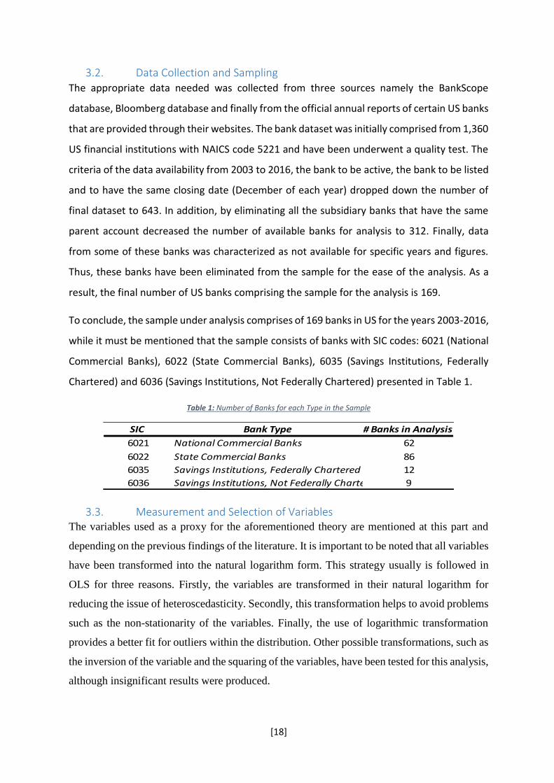
To conclude, the sample under analysis comprises of 169 banks in US for the years 2003-2016,
while it must be mentioned that the sample consists of banks with SIC codes: 6021 (National
Commercial Banks), 6022 (State Commercial Banks), 6035 (Savings Institutions, Federally
Chartered) and 6036 (Savings Institutions, Not Federally Chartered) presented in Table 1.
Table 1: Number of Banks for each Type in the Sample
3.3. Measurement and Selection of Variables The variables used as a proxy for the aforementioned theory are mentioned at this part and
depending on the previous findings of the literature. It is important to be noted that all variables
have been transformed into the natural logarithm form. This strategy usually is followed in
OLS for three reasons. Firstly, the variables are transformed in their natural logarithm for
reducing the issue of heteroscedasticity. Secondly, this transformation helps to avoid problems
such as the non-stationarity of the variables. Finally, the use of logarithmic transformation
provides a better fit for outliers within the distribution. Other possible transformations, such as
the inversion of the variable and the squaring of the variables, have been tested for this analysis,
although insignificant results were produced.
SIC Bank Type # Banks in Analysis
6021 National Commercial Banks 62
6022 State Commercial Banks 86
6035 Savings Institutions, Federally Chartered 12
6036 Savings Institutions, Not Federally Chartered 9

[19]
3.3.1. Explained Variable
The analysis will be performed with the use of the variable of Return on Average Equity
(ROAE) as a dependent variable. According to prior literature, the two most used variables as
proxies for bank profitability are the ROAE and ROAA (Staikouras and Wood, 2004; Zhang,
2016; Fukuyama and Matusek, 2017). In this analysis, the ROAE variable is used in its natural
logarithmic transformation for achieving a better fit with the rest variables of the estimated
model.
3.3.2. Independent Variables
LNIM is defined as the natural logarithm of Net Interest Margin. This is a variable used as a
proxy for bank’s liquidity risk. As it was already been mentioned an increase in the liquidity
risk of the bank will have a negative impact on the bank performance (Molyneux and Thornton,
1992; Abreu and Medes, 2001; Pasiouras and Kosmidou, 2007; Poi et al. 2017). Thus, a bank,
in cases that faces problems, will try to increase its liquid assets and reduce the liquidity risk.
In that notion the logarithm of net interest margin is being used as a proxy for liquidity risk,
because when the bank will manage to increase its liquidity assets and reduce the
corresponding risk, it will have manage to increase the net interest margin. As a result, an
increase in net interest margin would mean an increase in the bank performance (profitability).
Consequently, the expected relationship is positive with LROAE.
In the same notion, LTAR is being used. LTAR is the natural logarithm of Loans to Total
Assets Ratio and is used as a proxy for credit risk. The relationship of bank performance and
credit risk has been found by prior literature to be negative (Miller and Noulas, 1997; Flamini
et al., 2009; Goddard et al., 2010; Daly and Frikha, 2017). Meaning that an increase in the
credit risk of the bank will lead to reduce of its performance. That could be explained by the
fact that when financial institutions are exposed to high-risk loans, the accumulation of unpaid
loans increases, implying that these loan losses have produce lower returns to many
commercial banks. Thus, the expected relationship between the LTAR and LROAE is negative.
The next variable used as a proxy for the size of the bank is LTA, which is defined as the
natural logarithm of total assets of the bank. The relationship between the bank performance
and bank size has been analyzed in prior researches and it is expected the coefficient for LTA
to be positive (Bikker and Hu, 2002; Goddard et al., 2004; Goddard et al., 2010; Chowdhury
et al., 2017). Meaning that as the size of the bank increases, its profitability will increase too.
The capital of the bank is closely connected with its size. Meaning that if a bank is large
enough, would be easier to attract fund for increasing its capital. In that manner, the two

[20]
variables used as proxies for capital in this analysis, LETA (Natural Logarithm of Equity to
Total Assets Ratio) and LCAR (Natural Logarithm of Capital Adequacy Ratio), would have
the same impact as the size does on bank performance (Bennaceur and Goaied, 2008; Dietrich
and Wanzenried, 2011; Laeven et al., 2016). Thus, the relationship between the capital of the
bank and its profitability is expected to be positive.
Finalizing with the internal (bank-specific) factors of the analysis, LCIR is used as a proxy for
the bank’s expenses management. LCIR is the natural logarithm of cost to income ratio. In the
notion that the better the expenses management of the bank is, the lower the expenses would
be and as a result the higher the performance would be (Bourke, 1989; Molyneux and Thornton,
1992; Athanasoglou et al., 2008; Beltratti and Stulz, 2009; Djalikov and Piesse, 2016), the
expected relationship for this variable is negative.
Regarding the macroeconomic factors, three variables are being used as proxies, namely the
LINFLA, LIR and LGDPPCGR. These are the natural logarithm of inflation rate, of long-term
interest rate and gross domestic product per capital growth respectively. According to prior
literature, good economic conditions mean favorable economic environment for the entity
(bank) (Demirguc-Kunt and Huizinga, 2000; Bikker and Hu, 2002; Alper and Anbar, 2011;
Mergaerts and Vennet, 2016). That would lead to the increase of the bank performance, so the
expected relationship of these variables with the bank profitability is positive.
Overall, most studies’ results comply with the theory and the expected relationship of each
variable in this analysis is based on that. The expected impact of each variable is being
summarized in the next table (Table 2).
Table 2: Expected Relationship of each Group of Variables
Variable Indicator Measurement Expected Impact
LROAE Natural Logarithm of Return On Average Equity -
LNIM Natural Logarithm of Net Interest Margin Liquidity Risk +
LTAR Natural Logarithm of Loans to Assets Ratio Credit Risk -
LTA Natural Logarithm of Total Assets Size +
LETA Natural Logarithm of Equity to Total Assets ratio Capital +
LCAR Natural Logarithm of Capital Adequacy Ratio Capital +
LCIR Natural Logarithm of Cost to Income Ratio Expenses mngm. -
LINFLA Natural Logarithm of Inflation Macroeconomic +
LIR Natural Logarithm of Interest Rates Macroeconomic +
LGDPPCGR Natural Logarithm of Gross Domestic Product Per Capital Growth Macroeconomic +

[21]
3.4. Specification of the Model The first bank performance analysis has been undertaken by Short (1979), who investigated
the bank profitability. One of the latest and more complete empirical analysis in the field of
bank performance is the one from Dietrich and Wanzenried (2011), who used a panel analysis
of the data obtained for a number of financial institutions and for a specific period. Dietrich
and Wanzenried (2011) divided the sample it into two sub-periods in order to capture the
alterations of the determinants during the two specific periods. In the same notion this study
bases its analysis on the first bank performance model of Short (1979) and in order to capture
the crisis effect it bases its analysis on Dietrich and Wanzenried (2011) model. Furthermore,
some modifications are implemented in order to able to investigate all the groups of factors
affecting the bank performance. The modification involves the incorporation of all studied
determinants together, the internal and external factors, namely the bank-specific and the
macroeconomic factors.
The population regression function it is written as:
yi = β0+β1 χi + εi , i=1, 2, 3, …, n (1)
This formula divides the value of the dependent variable into two parts: the fitted value from
the model and an error term εi ~ i.i.d. Ν (0,σ2). Furthermore, according to Brooks (2008), since
Ordinary Least Squares is being put to use, a model with linear connection between the
parameters and not multiplied, divided, squared, or cubed, is needed. Thus, the final model that
it is going to be the base of the analysis is the following:
𝑌𝑖,𝑡 = 𝑐 + ∑ 𝑏𝑛𝑧𝑖,𝑡𝑛𝑁
𝑛=1 + ∑ 𝑏𝑘𝑧𝑖,𝑡𝑘𝐾
𝑘=1 + 𝜀 (2)
Where i: the ith bank and t the tth year and
Yi,t: Dependent variable measuring bank’s profitability (ROAΕ), of bank i at time t.
zn: Explanatory variable measuring the bank-specific factors affecting bank’s profitability.
zk: Explanatory variable measuring the macroeconomic factors affecting bank’s profitability.
c: Constant term
ε: Error term

[22]
Incorporating all the variables used for the analysis, in this model we have the final estimation
model:
𝐿𝑅𝑂𝐴𝐸𝑖𝑡 = 𝑐0 + 𝑐1𝐿𝐶𝐴𝑅𝑖𝑡 + 𝑐2𝐿𝐶𝐼𝑅𝑖𝑡 + 𝑐3𝐿𝐸𝑇𝐴𝑖𝑡 + 𝑐4𝐿𝑁𝐼𝑀𝑖𝑡 + 𝑐5𝐿𝑇𝐴𝑖𝑡 + 𝑐6𝐿𝑇𝐴𝑅𝑖𝑡 +
𝑐7𝐿𝐺𝐷𝑃𝑃𝐶𝐺𝑅𝑖𝑡 + 𝑐8𝐿𝐼𝑁𝐹𝐿𝐴𝑖𝑡 + 𝑐9𝐿𝐼𝑅𝑖𝑡 + 𝑐10𝑌𝐸𝐴𝑅𝑖𝑡 (3)
Where i: the ith bank and t: the tth year, and
LROAE: Natural Logarithm of Return on Average Equity
LCAR: Natural Logarithm of Capital Adequacy Ratio
LCIR: Natural Logarithm of Cost to Income Ratio
LETA: Natural Logarithm of Equity to Total Assets ratio
LNIM: Natural Logarithm of Net Interest Margin
LTA: Natural Logarithm of Total Assets
LTAR: Natural Logarithm of Loans to Assets Ratio
LGDPPCGR: Natural Logarithm of Gross Domestic Product per Capital Growth
LINFLA: Natural Logarithm of Inflation
LIR: Natural Logarithm of Interest Rates
YEAR: Year Dummy Variables

[23]
4. EMPIRICAL RESULTS AND DISCUSSION As already mentioned, the recent financial crisis effects on banks’ performance can be
determined by including in this analysis three different periods; the pre-crisis period, referring
to the years from 2003 to 2007, the post-crisis period, referring to period 2008-2016 and finally
the total sample period (2003-2016). Firstly, the descriptive statistics of each sample is
reported. Furthermore, the correlation matrix is presented to check for correlations between the
variables. Finally the regression analysis of all the aforementioned periods is performed, in
order to determine the factors affecting the bank profitability in the US and their alterations
during the years. Finally, the discussion of the analysis’ results are performed.
4.1. Descriptive Statistics As it is already been mentioned, the analysis will start with the presentation of the descriptive
statistics for the full sample and the two sub-samples. These statistics will provide us with
information about the distribution of the variables and will show us how each variable behaves
through time. Thus, it will help us to obtain a general idea of how the banks performed on
average for each period and as a total. The results are depicted in the following table (Table 3)
and are being analyzed. The figures are expressed in their initial form (percentages and billions
of dollars accordingly), in order to capture their meaning the important statistics easier.
Table 3: Descriptive Statistics for the Pre-Crises Sample (2003-2007)
As it is presented in the above table (Table 3), the pre-crises sample is comprised of 845
observations. The average of ROAE is 12.9% with a standard deviation of 4.8%, denoting that
on average the banks performed well with a return of 12.9%. The maximum ROAE observed
from a bank for the pre-crises period is almost 45%, while the minimum was -14.1%.
ROAE CAR CIR ETA NIM TA LTAR GDPPCGR INFLA IR
Mean 0.129 0.129 0.598 0.092 0.039 38.962 0.650 0.052 0.030 0.033
Median 0.129 0.111 0.600 0.089 0.039 25.411 0.677 0.057 0.033 0.029
Maximum 0.447 8.430 1.038 0.220 0.070 218.763 0.874 0.063 0.041 0.052
Minimum -0.141 0.068 0.230 0.047 0.010 22.946 0.049 0.035 0.019 0.015
Std. Dev. 0.048 0.289 0.099 0.024 0.008 19.251 0.128 0.010 0.008 0.015
Skewness 0.718 28.194 -0.195 2.080 -0.049 7.467 -1.328 -0.710 -0.212 0.204
Kurtosis 8.891 810.925 4.686 10.024 4.507 62.525 5.632 2.213 1.857 1.351
Jarque-Bera 1294 230939 105 2346 80 132603 492 93 52 102
Probability 0.00 0.00 0.00 0.00 0.00 0.00 0.00 0.00 0.00 0.00
Sum 109 109 505 78 33 329 550 44 25.65 27.88
Sum Sq. Dev. 1.98 70.34 8.23 0.48 0.05 31 14 0 0.05 0.18
Observations 845 845 845 845 845 845 845 845 845 845
Descriptive Statistics | Pre-Crises Sample (2003-2007)

[24]
Accordingly, we can see that banks for this specific period had on average 13% Capital
Adequacy Ratio, denoting a viable bank in terms of capital adequacy according to the Basel
Committee requirements. The variation in the CAR it can be observed from a minimum of
6.8% to 843%, meaning that surely there are banks that do not comply with the requirements.
The 60% Cost to Income Ratio, 9.2% Equity to Total Assets, 4% Net Interest Margin, 38.96
billions of dollars in Total Assets and 65% Loans to Assets Ratio, denote a normal performance
group of banks, on average for that period. The GDP per capital growth rate for that period
was on average 5.2%, while the inflation rate and interest rate showed on average a figure of
almost 3% each. The macroeconomic variables show on average a normal economic condition
for US, with low inflation and interest rate. It worth to be mentioned that all the variables do
not follow the normal distribution since the probability of J-B statistic is equal to 0 for all
variables. However, the non-normality is accepted for our analysis as it was expected.
Table 4: Descriptive Statistics for the Post-Crises Sample (2008-2016)
Turning to the post-crises sample, we analyze the variables of interest for the years of 2008-
2016. The results of the descriptive statistics are presented in the above table (Table 4). It can
be seen that the average ROAE dropped to 6.2% for the banks, meaning that the performance
of banks dropped down on average by 6.7%. The minimum return was -133% and the
maximum return was 75%. Thus, we can easily observe a higher variability in the returns
through the post-crises period. That can be ensured from the standard deviation figure (12.7%)
that is higher compared to the pre-crises period. The rest of the variables show little variation
through the years. Specifically, on average the CAR increased to 13.5%, which is again
compliant with the Basel Committee requirements. The CIR increased to 65.3%, ETA to 10.5%
ROAE CAR CIR ETA NIM TA LTAR GDPPCGR INFLA IR
Mean 0.062 0.135 0.653 0.105 0.036 63.989 0.640 0.020 0.031 0.019
Median 0.084 0.128 0.639 0.103 0.036 43.754 0.661 0.029 0.021 0.020
Maximum 0.745 3.496 7.399 0.585 0.068 257.277 0.955 0.034 0.076 0.031
Minimum -1.332 0.048 0.265 0.017 0.009 2.813 0.046 -0.029 0.001 0.012
Std. Dev. 0.127 0.091 0.228 0.026 0.007 30.213 0.127 0.019 0.025 0.006
Skewness -4.594 33.113 18.634 4.205 0.043 6.328 -1.170 -1.844 0.981 0.471
Kurtosis 36.256 1221.007 522.180 76.049 5.168 42.924 5.316 5.096 2.503 2.329
Jarque-Bera 75439 94297320 17170634 342662 298 111168 687 1140 259 85
Probability 0.00 0.00 0.00 0.00 0.00 0.00 0.00 0.00 0.00 0.00
Sum 94.69 205.07 993.51 160.00 54.79 97 973 31 46.44 29.50
Sum Sq. Dev. 24.57 12.61 78.96 1.05 0.07 139 25 1 0.93 0.05
Observations 1521 1521 1521 1521 1521 1521 1521 1521 1521 1521
Descriptive Statistics | Post-Crises Sample (2008-2016)

[25]
and TA increased to almost 64 billion, while NIM remained almost stable at 3.6% and LTAR
decreased to 64%, meaning that in spite of the financial crises, most banks on average retained
their viable condition. Finally, the GDP per capital growth decreased its figure to 2% on
average. Inflation remained stable, while the IR dropped down to 2%, denoting that the
macroeconomic environment did not remain stable but through the years worsened. Finally,
once again all the variables do not follow the normal distribution since the probability of J-B
statistic is equal to 0 for all variables. However, the non-normality is accepted for our analysis
as it was expected.
Nevertheless, in order to have a most holistic opinion of the situation through these years of
the analysis, the full sample for all the years must be presented and analyzed. The main
descriptive statistics are presented in the following table (Table 5).
Table 5: Descriptive Statistics for the Total Sample (2003-2016)
For the years 2003-2016, on average the banks showed a ROAE figure of 8.6%, meaning that
banks performed on average with a 9% return with a maximum value of 75% and a minimum
-133%. The variability during the whole period seems to be relatively high, producing a
standard deviation of the ROAE of 11.1%. The CAR figure of 64.4% shows a much higher
number than the lowest requirement set by the Basel Committee. The CIR figure of 10.1%,
ETA 13.3%, NIM 8.6%, denote a viable financial entity for the period from 2003 to 2016. The
average Total Assets for the banks was 55.05 billion and LTAR on average 3.7%, which show
again a viable economic entity. The average GDP per capital growth for US for the whole
period is 3.2%, while the inflation rate and interest rates produced on average 3% and 2.4%
respectively, denoting a good macroeconomic environment for the US banks. Finally, once
ROAE CAR CIR ETA NIM TA LTAR GDPPCGR INFLA IR
Mean 0.086 0.644 0.101 0.133 0.086 55.051 0.037 0.032 0.030 0.024
Median 0.097 0.666 0.098 0.123 0.097 36.263 0.037 0.031 0.026 0.021
Maximum 0.745 0.955 0.585 8.430 0.745 257.277 0.070 0.063 0.076 0.052
Minimum -1.332 0.046 0.017 0.048 -1.332 2.295 0.009 -0.029 0.001 0.012
Std. Dev. 0.111 0.128 0.026 0.187 0.111 26.840 0.007 0.022 0.020 0.012
Skewness -4.905 -1.224 3.346 39.226 -4.905 6.832 0.079 -1.090 1.137 1.295
Kurtosis 44.846 5.409 53.594 1672.913 44.846 50.734 4.766 4.529 3.545 3.624
Jarque-Bera 182119 1163 256758 275517 182119 243036 310 699 539 700
Probability 0.00 0.00 0.00 0.00 0.00 0.00 0.00 0.00 0.00 0.00
Sum 204 1523 238 314 204 130 87.80 75 72 57.38
Sum Sq. Dev. 28.99 38.53 1.62 82.97 29 170 0.13 1 0.98 0.33
Observations 2366 2366 2366 2366 2366 2366 2366 2366 2366 2366
Descriptive Statistics | Full Sample (2003-2016)

[26]
again all the variables do not follow the normal distribution since the probability of J-B statistic
is equal to 0 for all variables.
4.2. Correlations Continuing, it is necessary to perform a correlation analysis in order to obtain an idea of how
the variables are correlated with each other. The correlation coefficient matrices are presented
for the full sample and the sub-samples in the following tables (Tables 6, 7, 8). At this point,
the natural logarithms of the variables are used. In the same form as in the final regressions do.
Numbers in bold denote the statistically significant coefficients at 5% confidence level.
Analyzing all the correlation matrices, as most pairs of correlations show either a low or an
insignificant correlation, multicollinearity will not be an issue for most of the variables.
However, in order to be totally ensured about the existence of multicollinearity, a VIF-test was
performed and the results suggest that there is no multicollinearity.
Having analyzed the correlation coefficients concerning the multicollinearity problem, it is
time to have continued to the correlation coefficients analysis between the explained variable
(LROAE) and the explanatory variables.
Table 6: Correlation Coefficients for the Pre-Crises Sample (2003-2007)
Regarding the pre-crises period, many variables produce a positive correlation with the
dependent variable LROAE, meaning that an increase in the indicative paired explanatory
variable will lead to an increase in LROAE. Variables producing a positive relationship are the
LNIM, LTA, LINFLA and LGDPPCGR. The rest of the variables LCAR, LCIR, LETA, LTAR
and LIR. From all these variables, the LTA and LTAR produce a not statistically significant
correlation coefficient, so we cannot be sure for its reliability. It worth to be mentioned that all
the correlation coefficients show a relatively weak correlation between the dependent and the
respective explanatory variable, since they are no more than 0.25. The exception here is the
cost to income ratio that shows a relative medium negative correlation with a figure of almost
0.5. Besides the LROAE correlations with the variables we can observe that the strongest
LROAE LCAR LCIR LETA LNIM LTA LTAR LGDPPC LINFLA LIR
LROAE 1
LCAR -0.1710 1
LCIR -0.4806 -0.0230 1
LETA -0.2488 0.2797 -0.2527 1
LNIM 0.2528 -0.0326 -0.2417 0.3049 1
LTA 0.0765 -0.3177 -0.0979 0.0337 -0.3342 1
LTAR 0.0479 -0.3348 -0.0846 0.1113 0.5492 -0.2345 1
LGDPPC 0.1581 0.0872 -0.0706 -0.0859 0.1271 -0.0810 -0.1275 1
LINFLA -0.0683 -0.0733 0.0412 0.0522 -0.0806 0.0662 0.0921 -0.6580 1
LIR -0.0923 -0.0812 0.0478 0.0775 -0.1000 0.0792 0.1274 -0.8045 0.3262 1
Correlation Coefficient | Pre-Crises Sample (2003-2007)

[27]
correlation is between the macroeconomic factors (LGDPPC with LINFLA and LIR). The rest
of the variables show a medium or weak correlation with each other (no more than 0.35) except
the LNIM and LTAR.
Table 7: Correlation Coefficients for the Post-Crises Sample (2008-2016)
In the post-crises period we can observe that the results produced are slightly different. The
LROAE shows a positive relationship with LNIM, LTAR, LGDPGR and LINFLA, while a
negative relationship with the rest of the variables, namely LCAR, LCIR, LETA, LTA and
LIR. All correlation coefficients produce a statistically significant result except the LNIM,
LTAR and LIR. Once again, the correlation between the dependent and the explanatory
variables is weak with the strongest one to be -0.26 (LETA). Furthermore, the only strong
relationship for the post-crises period is observed between the LGDPPC and LINFLA and LIR.
The rest internal factors denote a medium or weak correlation among them with the strongest
being between LNIM and LTAR (0.52).
Table 8: Correlation Coefficient for the Full Sample (2003-2016)
Taking into consideration the full sample for the whole period from 2003 to 2016, we can
observe that all the correlation coefficients produce a statistically significant figure except the
LTAR variable. The ones producing a positive correlation are only LNIM, LTAR,
LGDPPCGR, LINFLA and LIR. The rest of the variables show a negative relationship with
LROAE. Finally, the variables show a relatively weak relationship with LROAE, with the
LROAE LCAR LCIR LETA LNIM LTA LTAR LGDPPC LINFLA LIR
LROAE 1
LCAR -0.1141 1
LCIR -0.1391 -0.0547 1
LETA -0.2643 0.4472 -0.1931 1
LNIM 0.0636 -0.0333 -0.1783 0.2019 1
LTA -0.0730 -0.1164 -0.1151 0.1716 -0.3649 1
LTAR -0.0087 -0.3827 -0.0585 0.1098 0.5191 -0.2844 1
LGDPPC 0.0304 0.2081 -0.0308 0.1194 -0.0048 0.0439 -0.0857 1
LINFLA 0.0464 0.1371 -0.0327 0.1514 -0.0539 0.0721 -0.0430 0.9026 1
LIR -0.0458 -0.2428 -0.0218 -0.1111 -0.0429 -0.0200 0.1020 -0.6740 -0.5342 1
Correlation Coefficient | Post-Crises Sample (2008-2016)
LROAE LCAR LCIR LETA LNIM LTA LTAR LGDPPC LINFLA LIR
LROAE 1
LCAR -0.1767 1
LCIR -0.2496 0.0027 1
LETA -0.3084 0.4116 -0.1519 1
LNIM 0.1476 -0.0694 -0.2244 0.1835 1
LTA -0.0796 -0.1561 -0.0741 0.1597 -0.3712 1
LTAR 0.0124 -0.3571 -0.0711 0.0990 0.5270 -0.2671 1
LGDPPC 0.2194 -0.0326 -0.1532 -0.1170 0.1277 -0.0980 -0.0475 1
LINFLA 0.0929 0.0394 -0.0612 0.0673 -0.0138 0.0267 -0.0188 0.7273 1
LIR 0.1018 -0.2473 -0.0923 -0.1554 0.0299 -0.0640 0.1095 -0.0380 -0.1433 1
Correlation Coefficient | Full Sample (2003-2016)
[28]
strongest one to be almost -0.31 (LETA). Finally, all the correlations between the variables
seem to be weak or medium with the strongest ones to be LNIM with LTAR (0.53) and
LGDPPC and LINFLA (0.73).
Overall, the descriptive statistics and correlation coefficients are an indication of the variables
moving and interaction. What we can surely expect from our analysis is that the highest impact
on the banks’ profitability will derive from the internal factors and specifically from the LCAR,
LETA and LCIR, while the LTA will have the weakest effect on the profitability. Finally, the
macroeconomic factors will have a significant role on the profitability, yet a weak one.
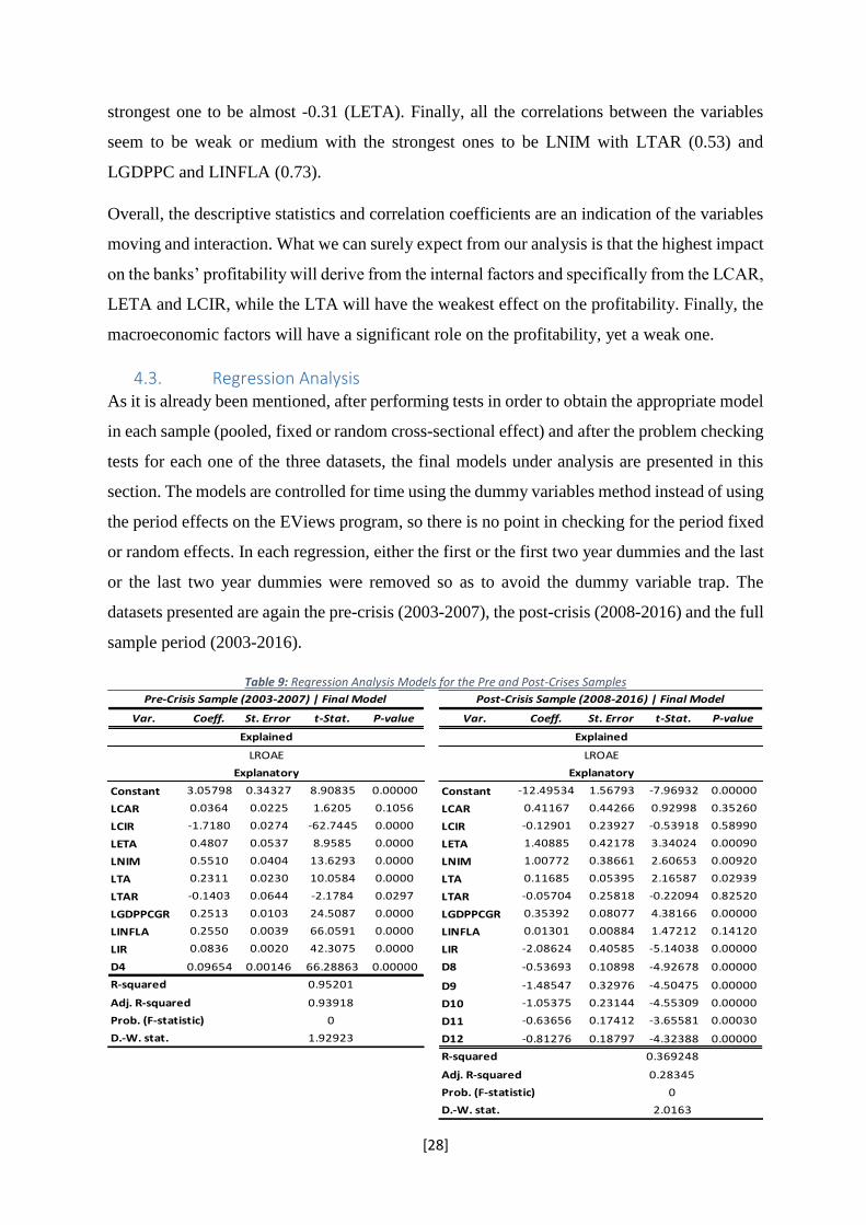
4.3. Regression Analysis As it is already been mentioned, after performing tests in order to obtain the appropriate model
in each sample (pooled, fixed or random cross-sectional effect) and after the problem checking
tests for each one of the three datasets, the final models under analysis are presented in this
section. The models are controlled for time using the dummy variables method instead of using
the period effects on the EViews program, so there is no point in checking for the period fixed
or random effects. In each regression, either the first or the first two year dummies and the last
or the last two year dummies were removed so as to avoid the dummy variable trap. The
datasets presented are again the pre-crisis (2003-2007), the post-crisis (2008-2016) and the full
sample period (2003-2016).
Table 9: Regression Analysis Models for the Pre and Post-Crises Samples
Var. Coeff. St. Error t-Stat. P-value Var. Coeff. St. Error t-Stat. P-value
Constant 3.05798 0.34327 8.90835 0.00000 Constant -12.49534 1.56793 -7.96932 0.00000
LCAR 0.0364 0.0225 1.6205 0.1056 LCAR 0.41167 0.44266 0.92998 0.35260
LCIR -1.7180 0.0274 -62.7445 0.0000 LCIR -0.12901 0.23927 -0.53918 0.58990
LETA 0.4807 0.0537 8.9585 0.0000 LETA 1.40885 0.42178 3.34024 0.00090
LNIM 0.5510 0.0404 13.6293 0.0000 LNIM 1.00772 0.38661 2.60653 0.00920
LTA 0.2311 0.0230 10.0584 0.0000 LTA 0.11685 0.05395 2.16587 0.02939
LTAR -0.1403 0.0644 -2.1784 0.0297 LTAR -0.05704 0.25818 -0.22094 0.82520
LGDPPCGR 0.2513 0.0103 24.5087 0.0000 LGDPPCGR 0.35392 0.08077 4.38166 0.00000
LINFLA 0.2550 0.0039 66.0591 0.0000 LINFLA 0.01301 0.00884 1.47212 0.14120
LIR 0.0836 0.0020 42.3075 0.0000 LIR -2.08624 0.40585 -5.14038 0.00000
D4 0.09654 0.00146 66.28863 0.00000 D8 -0.53693 0.10898 -4.92678 0.00000
D9 -1.48547 0.32976 -4.50475 0.00000
D10 -1.05375 0.23144 -4.55309 0.00000
D11 -0.63656 0.17412 -3.65581 0.00030
D12 -0.81276 0.18797 -4.32388 0.00000
Post-Crisis Sample (2008-2016) | Final Model
Explained
LROAE
Explanatory
R-squared
Adj. R-squared
Prob. (F-statistic)
D.-W. stat.
0.369248
0.28345
0
2.0163
Pre-Crisis Sample (2003-2007) | Final Model
LROAE
R-squared
Adj. R-squared
Prob. (F-statistic) 0
Explained
Explanatory
0.93918
0.95201
1.92923D.-W. stat.

[29]
In the above table (Table 9), the regression models for the pre-crises and the post-crises samples
are reported respectively.
Regarding the period from 2003 to 2007, the regression produced a R-squared of 95.2% and
adjusted R-squared 93.92%, meaning that the variation in the dependent variable is highly
explained (almost 95%) by the variation of the explanatory variables. A value of R2 almost
0.95 suggests that the deployed bank profitability model explains about 95% of the variance in
the Return on Average Equity. The unexplained part (5%) can be affiliated with two reasons,
with the circumstances that the model fails to explain or with the untested explanatory variables
(the variables not included in the model). The model’s probability of F-statistic (0.00) shows
the high significance of the model. Finally, the durbin-watson stat. is close to 2 (1.93), meaning
that there is no problem of autocorrelation in the residuals. In the same notion, the results for
the post-crises period (2008-2016) can be interpreted. The R-squared of the regression is
considerably lower at 37%, while the adj. R-squared is equal to 28%. However, the significance
of the model seems to be acceptable since the probability of the F-statistic is equal to 0. Finally,
the durbin-watson statistic is again close to 2 (2.01) and there is no presence of autocorrelation
in the residuals.
Regarding the explanatory variables, it can been seen that not all the bank profitability
determinants’ proxies, in both samples, are the same in the two samples. In the pre-crises
sample the LCIR and LTAR have a negative impact on the LROAE and as a result on the bank
profitability. The rest of the variables produce a positive effect on the dependent variable,
meaning that an increase in the aforementioned variables will lead in the increase of the
profitability. In addition, LCAR is not statistically significant, while the rest are significant.
Statistically significant at a 95% confidence level, or by using α=5%, is every variable that has
a prob. lower than 0.05. In the post-crises period we can observe some differences. The
variables LCIR, LTAR and LIR show a negative impact on the bank profitability
(performance) meaning that an increase in these variables will lead to a reduced performance
for the bank. The rest of the variables are producing a positive relationship with LROAE. The
statistically significant variables during that period are all of them except LTAR, LINFLA and
LCAR for α=5%.
Thus, there is a difference in what determines the bank performance in US prior and after the
financial crisis. More precisely, not only some of the variables that had a positive impact on
bank profitability changed to a negative impact, but the degree of the impact has changed too.
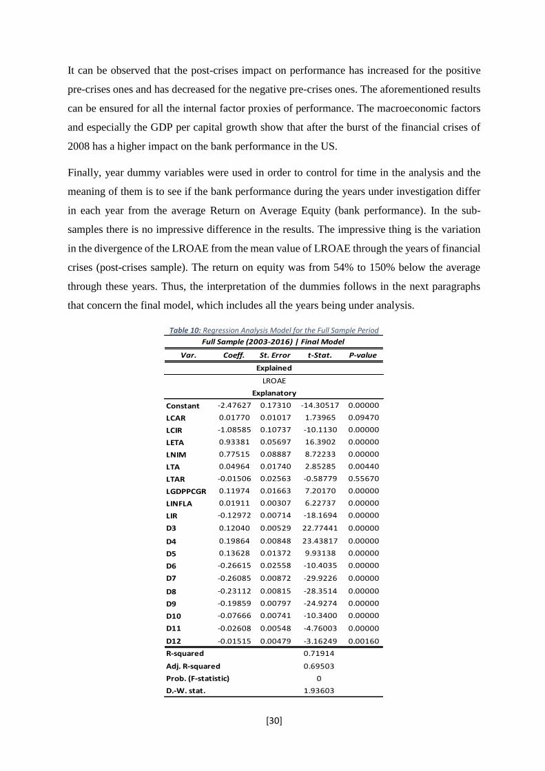
[30]
It can be observed that the post-crises impact on performance has increased for the positive
pre-crises ones and has decreased for the negative pre-crises ones. The aforementioned results
can be ensured for all the internal factor proxies of performance. The macroeconomic factors
and especially the GDP per capital growth show that after the burst of the financial crises of
2008 has a higher impact on the bank performance in the US.
Finally, year dummy variables were used in order to control for time in the analysis and the
meaning of them is to see if the bank performance during the years under investigation differ
in each year from the average Return on Average Equity (bank performance). In the sub-
samples there is no impressive difference in the results. The impressive thing is the variation
in the divergence of the LROAE from the mean value of LROAE through the years of financial
crises (post-crises sample). The return on equity was from 54% to 150% below the average
through these years. Thus, the interpretation of the dummies follows in the next paragraphs
that concern the final model, which includes all the years being under analysis.
Table 10: Regression Analysis Model for the Full Sample Period
Var. Coeff. St. Error t-Stat. P-value
Constant -2.47627 0.17310 -14.30517 0.00000
LCAR 0.01770 0.01017 1.73965 0.09470
LCIR -1.08585 0.10737 -10.1130 0.00000
LETA 0.93381 0.05697 16.3902 0.00000
LNIM 0.77515 0.08887 8.72233 0.00000
LTA 0.04964 0.01740 2.85285 0.00440
LTAR -0.01506 0.02563 -0.58779 0.55670
LGDPPCGR 0.11974 0.01663 7.20170 0.00000
LINFLA 0.01911 0.00307 6.22737 0.00000
LIR -0.12972 0.00714 -18.1694 0.00000
D3 0.12040 0.00529 22.77441 0.00000
D4 0.19864 0.00848 23.43817 0.00000
D5 0.13628 0.01372 9.93138 0.00000
D6 -0.26615 0.02558 -10.4035 0.00000
D7 -0.26085 0.00872 -29.9226 0.00000
D8 -0.23112 0.00815 -28.3514 0.00000
D9 -0.19859 0.00797 -24.9274 0.00000
D10 -0.07666 0.00741 -10.3400 0.00000
D11 -0.02608 0.00548 -4.76003 0.00000
D12 -0.01515 0.00479 -3.16249 0.00160
D.-W. stat.
0.71914
0.69503
0
1.93603
R-squared
Adj. R-squared
Prob. (F-statistic)
Full Sample (2003-2016) | Final Model
Explained
LROAE
Explanatory

[31]
The results presented in the above table (Table 10), include all 169 US banks and 14 years of
data (2003-2016). Once again, a cross-section fixed effect model was used as the most
appropriate for the analysis according to tests. The outcomes indicate a high significance model
the probability of F-statistic being equal to 0 and almost the 72% of LROAE variations are
explained by the variations in the explanatory variables, which can be considered as acceptable.
The rest 28% can be attributed to the explanatory variables not included in the model. That
could be the industry related factors that due to lack of data the appropriate variables have not
been incorporated in the model. The year dummies incorporated in the model are present for
the control of time, except the first two and the last two years for reasons mentioned in the
beginning of the analysis. Finally, the d-w stat. is again near to the value of 2 (1.94), which
denotes that the autocorrelation in the residuals is probably not present.
All the variables are statistically significant at 5% (prob. is lower than 0.05) except the LCAR
and the LTAR. However, LCAR is statistically significant for the level of α=10%. The
variables with a positive effect on audit fees are LCAR, LETA, LNIM, LTA, LINFLA and
GDPPCGR, while the ones with a negative effect are the LCIR, LTAR, LIR and the Constant.
That means that an increase of 1% in capital adequacy ratio, or in equity to assets, or in net
interest margin, or in total assets, or in inflation rate or in GDP per capital growth, will increase
the bank profitability by the respective percentage of the coefficient of the respective variable
and vice versa. For example, an increase of 1% in CAR will lead to an increase of ROAE by
almost 0.018%. On the other hand, an increase in the cost to income ratio or in loans to assets
ratio, or in long-term interest rates will decrease the return on average equity and as a result
the bank performance and vice versa. For example, an in increase in the cost to income ratio
by 1% will lead to a 1.09% decrease in ROAE. The results are almost as expected according
to the theory and the previous literature besides the relationship of ROAE and the interest rates
that it seems to have a negative correlation using the model.
The year dummies used in this model in order to control for time are all statistically significant
at any level. The results indicate that during the first 5 years of the analysis until the 2008 (pre-
crises period) the return on average equity figures of banks were from 12% up to 20% higher
than the average, while after 2008 (post-crisis) were by 1.5% up to 26.6% below the average.
That depicts the differences on bank performance before and after the burst of the financial
crisis of 2008.

[32]
To summarize, concerning the internal factors of profitability we can see that the risk
management has a positive impact when reducing liquidity risk and a negative impact when
increasing credit risk. Thus, the better the risk management the higher the profitability. Size
and capital of the bank seem to have a positive impact on the bank performance. Finally, the
expenses the higher they are the lower the profitability meaning that the expenses management
has a significant effect on bank performance. Regarding the macroeconomic factors, GDP per
capital growth and inflation rates show a positive correlation with bank profitability. However,
the long-term interest rates seem to have a negative impact on bank profitability when increase
and that is opposed to prior literature and findings.
4.4. Discussion of the Results After performing the statistical and econometric analysis, it is time to compare our findings
with the prior literature and discuss various policy recommendations according to the results.
4.4.1. Comparison with Prior Findings
Previous researches have established the main determinants of the bank profitability. The
results of these researches can be summarized in Table 2 of this thesis and in the first 3 columns
of Table 11. These outcomes was the base of this analysis, used as a guide for what to be
expected as a result. Thus, comparing the findings of this specific analysis with prior literature
it can easily be observed that our findings totally agree with prior literature except the long-
term interest rates that it is found to have the exact opposite effect from what it was expected.
Table 11: Comparison of the Research Outcome
The interesting part of the results is the not so strong reaction of policy makers or of the bank
managers so as to avoid the decrease of the bank performance in US. In the next part some
policy recommendations or actions suggested to be taken are being cited.
Variable Measurement Expected Impact Research Findings
LROAE - N/A N/A
LNIM Liquidity Risk + +
LTAR Credit Risk - -
LTA Size + +
LETA Capital + +
LCAR Capital + +
LCIR Expenses mngm. - -
LINFLA Macroeconomic + +
LIR Macroeconomic + -
LGDPPCGR Macroeconomic + +

[33]
4.4.2. Policy Recommendations
The analysis outcome showed that the recent financial crises that outburst in 2008 had a
significant impact on the bank profitability. It can easily be derived the factors that used to
affect the profitability of a bank had changed. That led to the huge decrease of their
performance. As a result it is crucial for the banks to change their policies in order to be in a
more stable financial condition and achieve higher numbers of profitability.
Concerning the full period from 2003 to 2016 we can easily observe that there are internal and
external factors that affect the profitability of a bank. Since the external factors are not easily
managed by a bank as an individual, the suggestions in their managements and decisions would
concern only the internal factors that are more easily managed. Thus, as far as the internal
factors are concerned, the three most important factors affecting the bank profitability are the
capital management, liquidity risk management and expenses management. Since the expenses
management is the factor that is affecting the bank profitability the most, the results suggest
that banks in order to avoid decreasing their profitability, they should have a more efficient
expenses management program. Since the cost-to-income ratio it was used for the analysis it
is suggested that the banks should either increase their income or decrease their expenses.
Furthermore, the second important factor affecting the bank profitability is the risk
management, especially the liquidity risk management. Since the net interest margin affects
the profitability in a positive way by decreasing liquidity risk, it is recommended for the banks
to increase their net interest margin in order to increase their performance. Finally, the third
most important factor is the capital management of the bank in a way that a more effective
capital management will lead to increased performance. As the equity-to-assets ratio it was
used, it is recommended that banks must increase their equity or decrease their assets in order
to be more profitable. However, the results of the analysis denote that the size of the bank is
positively affecting the profitability, and so the decrease of the assets is not recommended. All
these could either be accomplished by the bank managements by taking the proper actions or
by a higher institution that is responsible for the financial institutions’ actions and policies.

[34]

[35]
5. CONCLUDING REMARKS The final section of the thesis is comprised of the conclusions derived from the analysis, the
limitations that appeared during this investigation and cites areas that could be the base for
further research in the bank profitability factors’ field.
5.1. Research Conclusions This investigation tries to shed light into the determinants of bank profitability in the US
context. Furthermore, the main aim of this research is twofold. Besides the determination of
the group of determinants that affect bank profitability, it tries to capture the alterations in these
determinants through the years of the recent financial crises of 2008. More specifically, this
thesis contributes to the literature by using all the group of factors affecting the bank
performance, namely the internal (bank-specific) and external (macroeconomic) factors, for
the recent years in order to capture the effect of the financial crises. Examining the disclosed
return on equity figures for the years 2003-2016 and in a special way of creating sub-samples
(pre and post-crises), provides evidence to the extent of what is important that banks must
consider in order to be more profitable.
By deploying a regression model for the 14 years of sample panel data, the results produced
interesting results. The four main groups of internal factors, namely size, capital, risk
management and expenses management, seem to have a positive impact on the bank
profitability in all periods (before crises, after crises and for the whole period), but with
different weights in each period. Suggesting that what can be considered as important in bank
profitability has changed through the years and that is probably due to the crises that the
banking system suffered from. Finally, the macroeconomic environment (external factor)
seems to have a significant role in the profitability of the bank as it was expected. However,
the effect of the changes in the outer environment of the banking system seems to affect the
performance of the banks in small figures.
The conjecture of the effect of the world financial crisis, it was also being tested and it seems
to have a severe impact on bank performance. The way that banks manage to increase their
profitability, is different compared to the pre-crisis period. The results suggest that all the
factors that had a negative impact on return on equity before the burst of the crises has now
been oppressed, while all the positive effect factors have been increased. Meaning that banks
managed to take measures in order to be protected. However, the number of returns after the
2008 seem to be significantly below the average of the whole period of 14 years, denoting a
significant decrease in bank performance.
[36]
5.2. Research Limitations Various limitations has risen during this research. Firstly, this investigation used the US bank
dataset that can be considered as an abundant database in terms of availability of data.
Nevertheless, difficulties in data collecting that are mentioned in various sections throughout
the analysis, have risen and the object of this study is limited to the listed banks from 2003 to
2016, so the representation of the conclusion could be considered limited as well. A nice
example of the difficulties faced was in the data availability for obtaining the industry related
necessary data. Thus, the variables utilized in the analysis may be numerous but not enough in
order to capture all the possible determinants of the bank profitability. Thus, the existence of
other factors, not being able to be identified and be put to test is highly probable. Finally, a
larger dataset with extended time-periods may be beneficiary as it was mentioned before, to
capture more events of the past (Sarbanes and Oxley Act), but the difficulties in managing such
a large and complex dataset would be very difficult.
5.3. Suggestions for Future Research The dataset of this investigation is comprised of variables for the timespan from 2003 to 2016.
The dataset could be, in future researches, be expanded backwards in order to capture more
significant events of the past. In addition, this dataset comprises only from listed banks,
meaning that all the small and medium banks have been eliminated from the analysis. The
determinants of bank performance could produce interesting results for those banks too.
Finally, more variables such as the industry-related factors must be incorporated in the models
used for the analysis in order to obtain a more holistic consensus about the bank performance.

[37]
REFERENCES Abreu, M., & Mendes, V., (2001), “Commercial bank interest margins and profitability:
evidence for some EU countries”, Preliminary Draft.
Alper, D., & Anbar, A. (2011), “Bank specific and macroeconomic determinants of
commercial bank profitability: empirical evidence from Turkey”, Business and Economics
Research Journal, 2(2), 139-152.
Anarfi, D., Abakah, E. J. A. and Boateng, E., (2016), “Determinants of Bank Profitability
in Ghana: New Evidence”, Asian Journal of Finance and Accounting, 8(2).
Athanasoglou, P. P., Brissimis, S. N., & Delis, M. D., (2008), “Bank-specific, industry-
specific and macroeconomic determinants of bank profitability”, Journal of International
Financial Markets, Institutions and Money, 18(2), 121-136.
Athanasoglou, P. P., Delis, M. D., & Staikouras, C. K. (2006), “Determinants of Bank
Profitability in the South Eastern European Region”, (No. 47). Bank of Greece.
Barth, J.R., Caprio, G., Levine, R., (2004), “Bank supervision and regulation: What works
best?”, Journal of Financial Intermediation, 13(2), 205-248.
Beltratti, A., & Stulz, R. M., (2009), “Why did some banks perform better during the credit
crisis? A cross-country study of the impact of governance and regulation”, (No. 15180).
National Bureau of Economic Research.
Bennaceur, S., & Goaied, M., (2008), “The determinants of commercial bank interest
margin and profitability: evidence from Tunisia”, Frontiers in Finance and Economics,
5(1), 106-130.
Berger, A. N. (1995), “The relationship between capital and earnings in banking”, Journal
of Money, Credit and Banking, 432-456.
Berger, A.N., Hannan, T.H., (1989), “The price-concentration relationship in banking”,
Review of Economics and Statistics, 71, 291-299.
Bikker, J.A., Hu, H., (2002), “Cyclical patterns in profits, provisioning and lending of
banks and procyclicality of the new Basel capital requirements”, BNL Quarterly Review,
221, 143-175.
Bourke, P. (1989), “Concentration and other determinants of bank profitability in Europe,
North America and Australia”, Journal of Banking & Finance, 13(1), 65-79.
Chowdhury, M. A. F., Haque, M. and Masih, M., (2017), “Re-Examining the Determinants
of Islamic Bank Performance: New Ecidence from Dynamic GMM, Quantile Regression,

[38]
and Wavelet Coherence Approaches”, Emerging Markets Finance and Trade, 53, 1519-
1534.
Cornett, M. M., McNutt, J. J., & Tehranian, H., (2010), “The Financial Crisis, Internal
Corporate Governance, and the Performance of Publicly-Traded US Bank Holding
Companies”, SSRN Working Paper Series.
Daly, S. & Frikha, M. (2017), “Determinants of bank Performance: Comparative Study
between Conventional and Islamic Banking in Bahrain”, Journal of the Knowledge
Economy, 8(2), 471-488.
Demirgüç-Kunt, A., & Huizinga, H. (1999), “Determinants of commercial bank interest
margins and profitability: some international evidence”, The World Bank Economic
Review, 13(2), 379-408.
Demirgüç-Kunt, A., & Huizinga, H. (2000), “Financial Structure and Bank Profitability”,
World Bank Policy Research Working Paper, (2430).
DeYoung, R., and T. Rice, (2004), “Non interest income and financial performance at US
commercial banks”, The Financial Review, 39, 101–127.
Dietrich, A., & Wanzenried, G. (2011), “Determinants of bank profitability before and
during the crisis: Evidence from Switzerland”, Journal of International Financial
Markets, Institutions and Money, 21(3), 307-327.
Djalilov, K. and Piesse, J., (2016), “Determinants of bank profitability in transition
countries: What matters most?, Research in International Bussiness and Finance, 38, 69-
82.
Flamini, V., McDonald, C. A. & Schumacher, L., (2009), “The Determinants of
Commercial Bank Profitability in Sub-Saharan Africa” (No. 09/15). International
Monetary Fund.
Fukuyama, H. and Matousek, R., (2017), “Modelling bank performance: A network DEA
approach”, European Journal of Operational Research, 259(2), 721-732.
García-Herrero, A., Gavilá, S., & Santabárbara, D. (2009), “What explains the low
profitability of Chinese banks?”, Journal of Banking & Finance, 33(11), 2080-2092.
Goddard, J., Liu, H., Molyneux, P., & Wilson, J. O. (2010), “Do Bank Profits Converge?”,
(No. 10004). Bangor Business School, Prifysgol Bangor University (Cymru/Wales).
Goddard, J., Molyneux, P., & Wilson, J. O. (2001), “European banking: efficiency,
technology and growth”, Wiley & Sons Ltd.

[39]
Goddard, J., Molyneux, P., & Wilson, J. O. (2004), “The profitability of European banks:
a cross‐sectional and dynamic panel analysis”, The Manchester School, 72(3), 363-381.
Haslem, J.A., (1968), “A statistical analysis of the relative profitability of commercial
banks”, Journal of Finance, 23, 167-176.
Kosmidou, K. (2008), “The determinants of banks' profits in Greece during the period of
EU financial integration”, Managerial Finance, 34(3), 146-159.
Kosmidou, K., Tanna, S., & Pasiouras, F. (2005), “Determinants of profitability of
domestic UK commercial banks: panel evidence from the period 1995-2002”, Money
Macro and Finance (MMF) Research Group Conference, 45.
Laeven, L., Ratnovski, L. and Tong, H., (2016), “Bank size, capital, and systemic risk:
Some international evidence”, Journal of Banking and Finance, 69, s25-s34.
Mergaerts, F. and Vennet, R. V, (2016), “Business models and bank performance: A long-
term perspective”, Journal of Financial Stability, 22, 57-75.
Miller, S.M., Noulas, A.G., (1997), “Portfolio mix and large-bank profitability in the
USA”, Applied Economics, 29(4), 505-512.
Molyneux, P., & Thornton, J. (1992), “Determinants of European bank profitability: A
note”, Journal of banking & Finance, 16(6), 1173-1178.
Pasiouras, F., & Kosmidou, K. (2007), “Factors influencing the profitability of domestic
and foreign commercial banks in the European Union”, Research in International Business
and Finance, 21(2), 222-237.
Perry, P. (1992), “Do banks gain or lose from inflation?”, Journal of Retail Banking, 14(2),
25-40.
Poi, H. S., Shamsher, M. and Ariff, M. (2017), “Determinants driving bank performance:
A comparison of two types of banks in the OIC”, Pacific-Basin Finance Journal, 43, 193-
203.
Revell, J., (1979), “Inflation and financial institutions”, Financial Times, London.
Short, B. K. (1979), “The relation between commercial bank profit rates and banking
concentration in Canada, Western Europe, and Japan”, Journal of Banking & Finance,
3(3), pp. 209-219.
Smirlock, M. (1985), “Evidence on the (Non) Relationship between Concentration and
Profitability in Banking”, Journal of Money, Credit and Banking, 17(1), 69-83.
Staikouras, C., & Wood, G. (2004), “The determinants of European bank profitability”,
International Business & Economics Research Journal, 3(6), 57-68.

[40]
Stiroh, K. J., & Rumble, A. (2006), “The dark side of diversification: The case of US
financial holding companies”, Journal of banking & finance, 30(8), 2131-2161.
Trujillo‐Ponce, A. (2013), “What determines the profitability of banks? Evidence from
Spain”, Accounting & Finance, 53(2), 561-586.
Xiao, Y. (2009), “French Banks Amid the Global Financial Crisis”, (No. 09/201).
International Monetary Fund.
Zhang, Z., Xie, L., Lu, X. and Zhang, Z., (2016), “Determinants of Financial Distress in
Large Financial Institutions: Evidence from U.S. Bank Holding Companies”,
Contemporary Economic Policy, 34(2), 250-267.
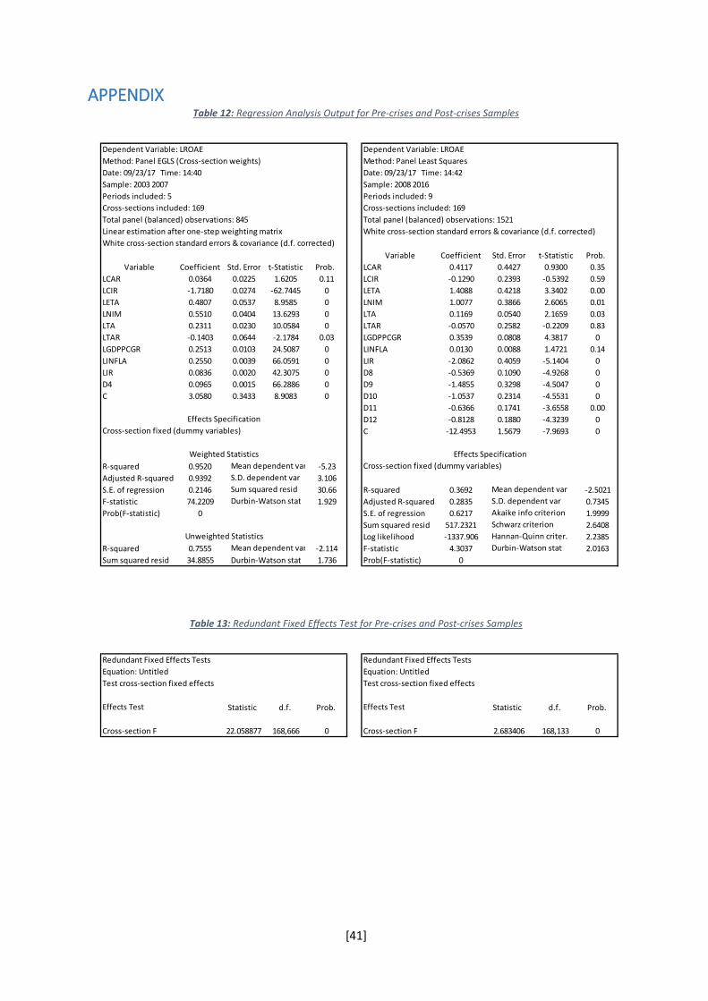
[41]
APPENDIX Table 12: Regression Analysis Output for Pre-crises and Post-crises Samples
Table 13: Redundant Fixed Effects Test for Pre-crises and Post-crises Samples
Variable Coefficient Std. Error t-Statistic Prob.
Variable Coefficient Std. Error t-Statistic Prob. LCAR 0.4117 0.4427 0.9300 0.35
LCAR 0.0364 0.0225 1.6205 0.11 LCIR -0.1290 0.2393 -0.5392 0.59
LCIR -1.7180 0.0274 -62.7445 0 LETA 1.4088 0.4218 3.3402 0.00
LETA 0.4807 0.0537 8.9585 0 LNIM 1.0077 0.3866 2.6065 0.01
LNIM 0.5510 0.0404 13.6293 0 LTA 0.1169 0.0540 2.1659 0.03
LTA 0.2311 0.0230 10.0584 0 LTAR -0.0570 0.2582 -0.2209 0.83
LTAR -0.1403 0.0644 -2.1784 0.03 LGDPPCGR 0.3539 0.0808 4.3817 0
LGDPPCGR 0.2513 0.0103 24.5087 0 LINFLA 0.0130 0.0088 1.4721 0.14
LINFLA 0.2550 0.0039 66.0591 0 LIR -2.0862 0.4059 -5.1404 0
LIR 0.0836 0.0020 42.3075 0 D8 -0.5369 0.1090 -4.9268 0
D4 0.0965 0.0015 66.2886 0 D9 -1.4855 0.3298 -4.5047 0
C 3.0580 0.3433 8.9083 0 D10 -1.0537 0.2314 -4.5531 0
D11 -0.6366 0.1741 -3.6558 0.00
D12 -0.8128 0.1880 -4.3239 0
C -12.4953 1.5679 -7.9693 0
R-squared 0.9520 -5.23
Adjusted R-squared 0.9392 3.106
S.E. of regression 0.2146 30.66 R-squared 0.3692 -2.5021
F-statistic 74.2209 1.929 Adjusted R-squared 0.2835 0.7345
Prob(F-statistic) 0 S.E. of regression 0.6217 1.9999
Sum squared resid 517.2321 2.6408
Log likelihood -1337.906 2.2385
R-squared 0.7555 -2.114 F-statistic 4.3037 2.0163
Sum squared resid 34.8855 1.736 Prob(F-statistic) 0
Akaike info criterion
Schwarz criterion
Hannan-Quinn criter.
Durbin-Watson stat
Effects Specification
Cross-section fixed (dummy variables)
Mean dependent var
S.D. dependent var
Mean dependent var
Durbin-Watson stat
Dependent Variable: LROAE
Method: Panel Least Squares
Date: 09/23/17 Time: 14:42
Sample: 2008 2016
Periods included: 9
Cross-sections included: 169
Total panel (balanced) observations: 1521
White cross-section standard errors & covariance (d.f. corrected)
Weighted Statistics
Mean dependent var
S.D. dependent var
Sum squared resid
Durbin-Watson stat
Unweighted Statistics
Total panel (balanced) observations: 845
Linear estimation after one-step weighting matrix
White cross-section standard errors & covariance (d.f. corrected)
Effects Specification
Cross-section fixed (dummy variables)
Dependent Variable: LROAE
Method: Panel EGLS (Cross-section weights)
Date: 09/23/17 Time: 14:40
Sample: 2003 2007
Periods included: 5
Cross-sections included: 169
Statistic d.f. Prob. Statistic d.f. Prob.
22.058877 168,666 0 2.683406 168,133 0
Effects Test
Cross-section F
Test cross-section fixed effects
Effects Test
Cross-section F
Redundant Fixed Effects Tests
Equation: Untitled
Test cross-section fixed effects
Redundant Fixed Effects Tests
Equation: Untitled

[42]
Table 14: Regression Analysis Output for Full Sample. No effects, Fixed Effects & Random Effects
Variable Coefficient Std. Error t-Statistic Prob. Variable Coefficient Std. Error t-Statistic Prob. Variable Coefficient Std. Error t-Statistic Prob.
LCAR -0.004232 0.034123 -0.12401 0.90 LCAR 0.017695 0.010171594 1.7396486 0.09 LCAR 0.007428 0.108771 0.068287 0.95
LCIR -0.984407 0.049011 -20.08525 0 LCIR -1.085854 0.107372 -10.11303 0 LCIR -0.685547 0.24793 -2.765085 0.01
LETA -1.001553 0.051004 -19.63661 0 LETA 0.933807 0.056973 16.39022 0 LETA -1.072872 0.153099 -7.007704 0
LNIM 0.602551 0.062903 9.579015 0 LNIM 0.775153 0.08887 8.722326 0 LNIM 0.741083 0.194828 3.803787 0.000
LTA 0.017778 0.006014 2.956261 0.003 LTA 0.049635 0.017398 2.852853 0.004 LTA 0.018052 0.023253 0.776315 0.44
LTAR -0.207536 0.03616 -5.73943 0 LTAR -0.015064 0.025629 -0.587786 0.56 LTAR -0.19388 0.070079 -2.766607 0.01
LGDPPCGR -0.047345 0.020024 -2.364375 0.02 LGDPPCGR 0.119735 0.016626 7.201696 0 LGDPPCGR -0.118936 0.038866 -3.060144 0.002
LINFLA 0.001277 0.003207 0.398252 0.69 LINFLA 0.019107 0.003068 6.227365 0 LINFLA -0.024551 0.003643 -6.738463 0
LIR -0.129824 0.006832 -19.00334 0 LIR -0.129721 0.00714 -18.16939 0 LIR -0.285536 0.013086 -21.81936 0
D3 0.137759 0.004356 31.62545 0 D3 0.120401 0.005287 22.77441 0 D3 0.216543 0.012236 17.69755 0
D4 0.210175 0.006432 32.67812 0 D4 0.198644 0.008475 23.43817 0 D4 0.364364 0.018824 19.3564 0
D5 0.169836 0.011228 15.12624 0 D5 0.136282 0.013722 9.931377 0 D5 0.223723 0.024149 9.264118 0
D6 -0.226933 0.027977 -8.111403 0 D6 -0.266147 0.025582 -10.40352 0 D6 -0.456134 0.077925 -5.853526 0
D7 -0.26466 0.008437 -31.36824 0 D7 -0.260845 0.008717 -29.92255 0 D7 -0.274119 0.021299 -12.87007 0
D8 -0.253593 0.006767 -37.47328 0 D8 -0.231118 0.008152 -28.35144 0 D8 -0.417039 0.03102 -13.44397 0
D9 -0.198143 0.005797 -34.17748 0 D9 -0.198594 0.007967 -24.92743 0 D9 -0.349889 0.038054 -9.194589 0
D10 -0.10422 0.004093 -25.46088 0 D10 -0.076661 0.007414 -10.34 0 D10 -0.289092 0.028872 -10.01278 0
D11 -0.031722 0.004346 -7.299698 0 D11 -0.026077 0.005478 -4.760027 0 D11 -0.096649 0.028635 -3.375173 0.001
D12 -0.009819 0.003995 -2.457722 0.01 D12 -0.015152 0.004791 -3.162491 0.002 D12 -0.078117 0.014819 -5.271537 0
C -4.128483 0.141683 -29.13892 0 C -2.476269 0.173103 -14.30517 0 C -4.596791 0.401177 -11.45825 0
R-squared 0.551261 -4.23 S.D. Rho
Adjusted R-squared 0.547627 2.680 0.18435 0.104
S.E. of regression 0.556411 726.3 0.542196 0.896
F-statistic 151.6833 1.310 R-squared 0.719144 -4.709
Prob(F-statistic) 0 Adjusted R-squared 0.69503 2.949
S.E. of regression 0.503496 552.1 R-squared 0.238559 -1.461
F-statistic 29.82282 1.686 Adjusted R-squared 0.232393 0.621
R-squared 0.246247 -2.364 Prob(F-statistic) 0 S.E. of regression 0.544146 694.6
Sum squared resid 787.2529 1.606 F-statistic 38.68431 1.787
Prob(F-statistic) 0
R-squared 0.364388 -2.364
Sum squared resid 663.8614 1.912
R-squared 0.254543 -2.36
Sum squared resid 778.5879 1.59
Unweighted Statistics
Mean dependent var
Unweighted Statistics Durbin-Watson stat
Mean dependent var
Durbin-Watson stat
Durbin-Watson stat S.D. dependent var
Mean dependent var Sum squared resid
Durbin-Watson stat Durbin-Watson stat
Mean dependent var
Weighted Statistics S.D. dependent var
Unweighted Statistics
Sum squared resid Mean dependent var
S.D. dependent var Cross-section random
Sum squared resid Weighted Statistics Idiosyncratic random
Durbin-Watson stat
Cross-section fixed (dummy variables)
Weighted Statistics Effects Specification Effects Specification
Mean dependent var
Linear estimation after one-step weighting matrix Linear estimation after one-step weighting matrix Swamy and Arora estimator of component variances
White cross-section standard errors & covariance (d.f. corrected) White cross-section standard errors & covariance (d.f. corrected) White cross-section standard errors & covariance (d.f. corrected)
Cross-sections included: 169 Cross-sections included: 169 Cross-sections included: 169
Total panel (balanced) observations: 2366 Total panel (balanced) observations: 2366 Total panel (balanced) observations: 2366
Sample: 2003 2016 Sample: 2003 2016 Sample: 2003 2016
Periods included: 14 Periods included: 14 Periods included: 14
Method: Panel EGLS (Cross-section weights) Method: Panel EGLS (Cross-section weights) Method: Panel EGLS (Cross-section random effects)
Date: 09/23/17 Time: 14:46 Date: 09/23/17 Time: 14:45 Date: 09/23/17 Time: 14:46
Dependent Variable: LROAE Dependent Variable: LROAE Dependent Variable: LROAE

[43]
Table 15: Redundant Fixed Effects Test and Random Effects Hausman Test
Chi-Sq. Statistic Chi-Sq. d.f. Prob.
17.223 19 0.02964
Statistic d.f. Prob.
8.533189 168,217 0
Effects Test
Cross-section F
Redundant Fixed Effects Tests
Equation: Untitled
Test cross-section fixed effects
Test Summary
Cross-section random
Equation: Untitled
Test cross-section random effects
Correlated Random Effects - Hausman Test