Financial Markets, Banks’ Cost of Funding, and Firms’

Decisions:

Lessons from Two Crises

PIERLUIGI BALDUZZI1, EMANUELE BRANCATI2, and FABIO SCHIANTARELLI3

This draft: August 9, 2016

ABSTRACT

We test whether adverse changes to banks’ market valuations during the financial and sovereigndebt crises affected firms’ real decisions. Using new data linking over 5,000 non-financial Italianfirms to their bank(s), we find that increases in banks’ CDS spreads, and decreases in their equityvaluations, resulted in lower investment, employment, and bank debt for younger and smaller firms.These effects dominate those of banks’ balance-sheet variables. Moreover, CDS spreads mattermore than equity valuations. Finally, higher CDS spreads led to lower aggregate investment andemployment, and to less efficient resource allocations, especially during the sovereign debt crisis.

JEL # E44, G01, E22, E24, G21

Keywords: Financial crisis, sovereign debt crisis, credit default swaps, investment, employment

1 Corresponding author, Boston College, Carroll School of Management, 140 Commonwealth Avenue, Chestnut Hill,

MA 02467, phone: 617-552-3976, e-mail: balduzzp@bc.edu. 2 LUISS Guido Carli University, Viale Romania 32,

Rome, Roma 00100, Italy, phone: 39-06-85225-550, e-mail: ebrancati@luiss.it. 3 Boston College, Economics Depart-

ment, 140 Commonwealth Avenue, Chestnut Hill, MA 02467, phone: 617-552-4512, e-mail: fabio.schiantarelli@bc.edu.

We thank Gaetano Antonetti, Kit Baum, Steve Bond, Riccardo De Bonis, Francesco Giavazzi, Luigi Guiso, Rony

Hamaui, Anil Kashyap, Amiyatosh Purnanandam, Jun Qian, David Roodman, Roberto Savona, Mark Schaffer,

Alessandro Sembenelli, Nicolas Serrano-Velarde, Phil Strahan, and Carmine Trecroci, for useful conversations. We

also thank seminar participants at Boston College (Economics and Finance), University of Brescia, Bocconi Univer-

sity, the Federal Reserve Bank of Boston, the Bank of Italy, the European University Institute, the OECD, the NBER

Summer Institute, Fordham University, the University of Zurich, the 2015 CESifo Conference on Macroeconomics

and Survey Data, and the 2016 WFA meetings for useful comments. Finally, we thank Monitoraggio Economia e

Territorio (MET) for providing the survey data that made this study possible, and Giacomo Candian for expert

research assistance.

Introduction

The financial and sovereign debt crises have generated substantial fluctuations in the market value

of individual banks, reflecting their differential exposures to U.S. assets or banks, and to Euro-

zone sovereign debt. This paper asks whether these fluctuations matter for firms’ investment and

employment and investigates the nature of the transmission mechanism of financial shocks to real

outcomes. Specifically, we address two questions. First, we ask whether two firms, identical in

terms of observable characteristics, made different real choices because of the financial valuations

of their lending banks, even after controlling for the bank’s fundamentals. Second, we ask whether

two firms borrowing from the same bank were impacted differently by the two crises depending

upon their age and/or size.

We address the questions above in the context of the financial and sovereign debt crises in

Italy. However, the relevance of our analysis goes beyond the recent Italian experience, as any

financial crisis has the potential to affect the real economy through its effects on banks’ financial

valuations. Importantly, this new form of the bank lending channel transmits financial shocks even

to privately held companies, as long as there are frictions in the substitution of bank credit with

other types of funding.

We argue that banks’ financial market valuations provide useful summary measures of bank

funding costs and, hence, of credit conditions for bank customers. As compared to the traditional

balance-sheet based measures of bank health typically used in the literature, financial market val-

uations have two advantages. First, they are forward-looking and they are likely to incorporate

more information than what is currently reflected in a bank’s balance-sheet variables. Second, they

embed information about a bank’s riskiness and aggregate risk and risk aversion and may also re-

flect “market dislocation” effects.1 It is likely that bank managers respond to all of these factors in

1Fleckenstein, Longstaff, and Lustig (2014) and Pasquariello (2014), for example, document pronounced mispricing

1

setting lending policies.

We concentrate on the banks’ Credit Default Swap (CDS) spread and Tobin’s Q as market-

based measures of bank’s health, and assess the impact of these measures on the investment, em-

ployment, and bank debt of client firms. The CDS spread captures banks’ cost of debt over and

above the risk-free rate; whereas Tobin’s Q directly measures the cost of equity capital, but at the

same time may also reflect borrowing costs. Both measures, although not necessarily to the same

degree, should capture the credit conditions faced by client firms.

Whereas several contributions have analyzed the effects of the financial crisis on bank lending,

there is more limited evidence about the resulting effects on firms’ real decisions.2 Even less is known

about the real effects of the sovereign debt crisis.3 To the best of our knowledge, this is the first

paper to provide evidence for both episodes, using a sample that includes micro and small Italian

firms, the more likely to be bank-dependent. As we will argue, Italy is an important laboratory to

study the effect of the two crises.

Studying the effects of the two crises on firms’ real decisions, investment and hiring, is

important because firms may have access to alternative sources of funds and, hence, may be able

to at least partly neutralize shocks to the availability and cost of bank funding (Adrian, Colla, and

Shin, 2012, and Becker and Ivashina, 2014). Our joint analysis of the effects of the two crises is

warranted because the two episodes are different in their origin and had different effects on banks’

health. Hence, it is natural to ask how the bank lending channel operated in each case and which

one of the two negative shocks had more severe real effects. By focusing on a sample that includes

small and micro firms, we are able to have accurate quantitative estimates of the real effects of the

across different markets during the financial crisis. Aizenmann, Hutchinson, and Jinjarak (2012) argue that thepricing of sovereign risk was “noisy” during the global crisis period and, especially, in 2010.

2See the studies by Chodorow-Reich (2014), for the U.S., Bentolila, Jansen, Jimenez, and Ruano (2013) for Spain,and Cingano, Manaresi, and Sette (2013) for Italy, which will be discussed in Section 1 below.

3Our paper, and the concurrent paper by Acharya, Eisert, Eufinger, and Hirsh (2014), which uses DealScan datafor large European firms, are, to our knowledge, the only contributions to date on this topic.

2

two crises. Conversely, limiting the analysis to large firms, as other studies have done, is likely to

lead to underestimating the importance of the bank lending channel.

Our empirical analysis focuses on the Italian economy between 2006 and 2013. Hence, our

sample starts immediately before the financial crisis and ends after the Italian sovereign debt crisis

was brought under control by the appointment of the Monti government, the introduction of the

ECB’s Long Term Re-financing Operations at the end of 2011, and Draghi’s “whatever it takes”

speech of July 26, 2012. There are several reasons why the Italian experience is instructive and

relevant. First, Italy is a country of central importance within the Eurozone and the largest economy

directly affected by the sovereign debt crisis (Italy’s GDP is approximately equal to the GDP of

Spain, Greece, Portugal, and Ireland, combined). Second, both crises can be viewed as shocks that

are largely exogenous to the Italian non-financial corporate sector, in contrast to countries such

as Ireland and Spain, where the crises originated with the burst of a real estate bubble and the

ensuing collapse of the domestic real estate and construction sectors. Third, the two crises generate

heterogeneous time variation in banks’ cost of funding, depending upon their exposure to U.S. banks

and Italian sovereign debt. This differential response allows us to estimate the effects of changes

in banks’ cost of funding on client firms’ real decisions. Fourth, Italian banks rely heavily on bond

issuance as a source of funding and, hence, are severely exposed to changes in the cost of debt.

Moreover, Italian banks had large holdings of Italian sovereign bonds: roughly 7% of their assets

in 2010.4 Fifth, Italian firms are predominantly small and privately held, and are largely unable

to cushion shocks to the cost and availability of bank lending by resorting to the capital markets.

Finally, Italian firms mainly finance themselves with variable-rate credit, a substantial fraction of

which is short-term, and, hence, are especially vulnerable to changes in the cost and availability of

bank funding.5

4Gennaioli, Martin, and Rossi (2014).5On the prevalence of variable-rate funding for Italian firms, see, for example, the supplement to the

3

In addressing the question above, we employ a newly available data set of over 5,000 Italian

firms. This data set includes a large number of privately held small and micro firms, and provides

information on the identity of the bank(s) each firm has a relationship with. This information

allows us to exploit the time variation of the cross-sectional differences in banks’ cost of funding to

identify the real effects of banks’ financial market valuations on borrowing firms.

Our data set provides a more comprehensive coverage of small and micro firms than other

data sets, such as the Credit Registry of the Bank of Italy. Indeed, small and micro firms (less than

20 employees) account for more than half of sales, value added, investment, and employment in the

Italian economy, for the crisis period 2008–2011.6 In addition, the vast majority of the firms in our

sample (over 80%) borrow from one bank only, which limits their ability to adjust to credit-supply

shocks.

We allow the effects of banks’ financial market valuations on firm’s decisions to depend on

the likelihood of the firm being financially constrained, as measured by age and size. Moreover,

we investigate whether other bank-related variables, in addition to our cost-of-funding measures,

impact firms’ decisions. We do so by including in the investment equation controls for bank balance-

sheet variables (Tier 1 capital ratio, liquidity, etc.) at the beginning of each period, as well as

expectations of banks’ fundamentals based on analysts’ earnings forecasts. Although our main

focus is on investment, we show that our basic results also hold for firms’ employment and bank

debt.

Obviously, Italian firms not only faced funding shocks, but were also exposed to the negative

demand shocks associated with the two crises. As in other studies of the bank lending channel, this

February 2015 Bank of Italy’s Statistical Bulletin: http://www.bancaditalia.it/pubblicazioni/moneta-banche/2015-moneta/en suppl 07 15.pdf?language id=1. As to debt maturity, for the firms in our sample, the median share ofshort-term (less than one year) bank borrowing is roughly 60% of total bank borrowing; see Section 4.3 for details.

6Authors’ calculations based on ISTAT data. At the EU level, the role of small and micro firms (less than 50employees) is equally important: as of 2009, they account for about 40% of value added (Eurostat).

4

creates a challenge in disentangling the effect of bank credit supply on firms’ decisions from the

effects of demand conditions. We address this central identification problem using a two-pronged

approach. First, we introduce in our regressions (that always contain firm-specific time invariant

effects) time-varying firm-level balance sheet variables and year fixed effects that, in the most

general specifications, are allowed to vary by industry, region, age, size, export status, and bank-

size.7 Moreover, for the subset of firms with a single banking relationship, we can also control for

time-varying unobservable bank-specific characteristics.8

Second, we develop an instrumenting strategy in the context of a GMM estimator (see, for

example, Arellano and Bond, 1991; and Blundell and Bond, 1998).9 The need to instrument banks’

financial valuations may still arise because of their potential endogeneity due, for instance, to omit-

ted variables and reverse-causality effects: banks’ financial market conditions could be correlated

with omitted unobservable variables in the investment, employment, and bank-debt equations, and

could be themselves affected by the choices of client firms. Moreover, the firm-level variables that

we use to control for firm’s investment opportunities are also likely to be correlated with the error

term.

We go beyond the standard use in dynamic panels of appropriately lagged values of the

regressors as internal instruments. More precisely, we instrument banks’ valuations with their pre-

crisis exposure to dollar-denominated assets—interacted with the (lagged) CDS spread on U.S.

banks—and with their exposure to sovereign bonds—interacted with the (lagged) CDS spread on

Italian Treasury bonds. In other words, we use the fact that banks’ market valuations respond

differently to the two crises, depending upon banks’ exposures to the two types of risky assets.

7Note that the predominance of single firm-bank relationships in our sample prevents us from implementing theKhwaja and Mian (2008) within-firm estimator when we model firms’ bank debt. Hence, we are also unable to use theresulting estimates to control for demand effects in specifications for single firm-level outcomes, such as investmentand employment. See the end of Section 3.3.1 for a discussion of these issues.

8Note, though, that in this case we can only estimate how the effect of banks’ market valuations differs acrosstypes of firms.

9A detailed discussion of our econometric technique is contained in Section 3.

5

Our identifying assumption is that these interacted exposures are orthogonal to the idiosyncratic

shocks to firms’ decisions. The use of pre-crisis exposures deals with possible feedback from firms’

decisions to bank portfolio choices. Furthermore, even though the financial and sovereign debt

crises originated outside the Italian non-financial corporate sector, the use of lagged—as opposed

to contemporaneous—CDS spreads represents an extra degree of caution in instrument selection.

The main results of the empirical analysis are easily summarized: an increase in a bank’s

CDS spread, CDS volatility, and stock price volatility, and a decline in Tobin’s Q, all affect the

investment activity of client firms. Ceteris paribus, these effects are negative and significant for

younger and smaller firms. For example, for the CDS spread, the effect is negative and significant

for firms up to 8 years of age, which represent the 29th percentile of the age distribution. The effect

is also economically significant: after controlling for firm-specific effects and common year effects,

a one-standard deviation increase in a bank’s CDS spread decreases the investment activity of a

client firm at the 10th percentile of the age distribution—a three-year old firm—by 0.5 standard

deviations. On the other hand, the effect is insignificant, or even mildly positive, for the oldest

firms. This result underscores the importance of including young (small) firms in the sample. If

we only focused on older (larger) firms, we would erroneously conclude that the the two crises had

no adverse effects on capital accumulation through the bank lending channel. We also document

significant negative effects of changes in the CDS spread on employment and bank debt of younger

and smaller firms. Therefore, there is evidence of a bank lending channel in the transmission of

adverse financial shocks, characterized by a flight away from more informationally opaque borrowers.

The results above are robust to the inclusion of a variety of controls for firms’ investment

opportunities and creditworthiness. Importantly, while bank balance-sheet fundamentals enter the

construction of the two external instruments described earlier, they do not matter as additional

covariates. The beginning-of-period amounts of dollar-denominated assets, sovereign bond holdings,

6

and liquid assets, the Tier-1 capital ratio, and the amounts of deposits and charge-offs, are largely

insignificant, after controlling for the market-based cost-of-funding measures. Among the bank

cost-of-funding measures used in our empirical work, the banks’ CDS spread dominate Tobin’s Q,

suggesting that debt, rather than equity, is the marginal source of funding for the banks in our

sample, and that CDS spreads are the better measure of banks’ borrowing costs. Moreover, both

the level and the (orthogonalized) volatility of CDS spreads matter. Finally, adverse financial shocks

also have a negative impact on the employment and bank debt of young and small firms.

While our econometric analysis is performed at the firm level, we also investigate the aggre-

gate implications of our results. Specifically, we compute the deviation of actual firm investment

and employment from the counterfactual investment and employment, had the CDS spread of the

lender bank(s) stayed at the previous year’s level. We then aggregate across firms to compute the

aggregate effect of CDS changes, and we relate the aggregate effect to the average aggregate stock

of capital or aggregate employment over the two years. Furthermore, we compute indicators of

allocative efficiency for both investment and net employment changes: we relate the correlation

of the marginal-revenue product of capital (labor) with actual investment (employment changes)

to the correlation with counterfactual investment (employment changes). The increase in banks’

CDS spreads after the financial crisis and the even larger one during the sovereign debt crisis led

to a net reduction in the aggregate investment rate that was particularly substantial in 2011, when

banks’ valuations were severely affected. In all years, but 2013, actual investment is allocated less

efficiently than counterfactual investment, with the more pronounced efficiency losses in 2008, and

2011-2012. As to employment decisions, the changes in banks’ CDS spreads led to negative ag-

gregate employment growth in all years, but 2013, and the employment losses are largest in 2011

and 2012. In all years, but 2013, the allocation of net employment changes is less efficient than the

counterfactual allocation, with the largest efficiency loss also in 2011-2012. Therefore, the aggregate

7

effects of the bank-lending-channel are more pronounced for the sovereign debt crisis than for the

financial crisis.

In summary, our paper provides several novel findings. First, the two crises had significant

real effects through the bank lending channel, which operated mainly through the banks’ cost of

funding, as measured by the banks’ financial market valuations. However, given the dynamics

of CDS spreads and equity market valuations, the adverse effects of the sovereign debt crisis on

both investment and employment were much larger than those generated by the financial crisis.

Moreover, banks’ financial market valuations dominate balance-sheet variables and still matter over

and above analysts’ earnings forecasts. Finally, CDS spreads matter more than equity valuations.

Overall, we highlight an important channel through which financial market shocks affect the real

economy. Even in countries where the fraction of firms with publicly traded financial instruments

is small, financial market fluctuations may have a powerful impact on firms’ real decisions, through

their effect on banks’ cost of funding, and, hence, on the lending conditions to firms. Moreover,

shocks to banks’ financial valuations matter over and above measurable banks’ fundamentals.

The structure of the paper is as follows. Section 1 further discusses our contribution to the

existing literature. Section 3 presents the empirical methodology we use, with an emphasis on how

we deal with possible endogeneity issues. Section 4 describes the data and, in particular, the novel

survey data set containing the information on firm-bank relations used in the analysis. Section 5

discusses the empirical results. Section 6 explores the aggregate implications of the analysis. Section

7 concludes the paper.

8

1 Related literature

Although our paper focuses on the real effects of the bank lending channel, it builds on and com-

plements the rich set of contributions that analyze the effect of the financial crisis and the sovereign

debt crisis on bank credit.10 Ivashina and Scharfstein (2010), for example, document that U.S.

banks reduced their lending more during the crisis, if they had a less stable deposit base, or if

they were more exposed to credit-lines drawdowns because of co-syndicated loans with Lehman

Brothers.11

In an international context, Puri, Rocholl, and Steffen (2011) show that more loan applica-

tions were rejected by German banks, if these banks had holdings in Landesbanken with substantial

U.S. subprime exposure. Jimenez, Ongena, Peydro, and Saurina (2012a,b) use Spanish data to show

that banks’ capitalization and liquidity matter for the probability of obtaining a loan in time of crisis

and for the transmission of monetary policy.12 Iyer, Peydro, da Rocha-Lopes, and Schoar (2014),

on the other hand, use Portuguese data to show that banks relying more on interbank borrowing

before the crisis, decreased their credit supply more during the crisis. Moreover, the contraction in

credit supply was stronger for smaller firms with weaker banking relationships. Two recent papers

have focused on the effects of the sovereign debt crisis: Popov and Van Horen (2013) and De Marco

(2013), using data from the European Banking Authority, show that banks with higher exposure

to sovereign shocks tighten credit supply by more than less exposed banks.

Focusing on the Italian experience during the financial crisis, Albertazzi and Marchetti (2010)

10These papers, in their emphasis on banks’ balance-sheet variables, build on the earlier contributions on theimportance of the bank lending channel of monetary policy by Kashyap, Stein, and Wilcox (1993), and Kashyapand Stein (2000). They also build on Peek and Rosengren (1997, 2000), who study the international transmissionof bank-credit supply shocks following the stock market and real estate crashes in Japan. Another example of banklending response to external shocks is the impact of nuclear tests in Pakistan, studied by Khwaja and Mian (2008).

11See also Cornett, McNutt, Strahan, and Tehranian (2011), who emphasize the importance of core deposits, andMontoriol-Garriga and Wang (2011), who document the deterioration of access to credit for small firms during theGreat Recession.

12Jimenez, Mian, Peydro, and Saurina (2014) show that banks’ ability to securitize real estate assets enabled themto expand credit supply more, prior to the crisis.

9

and Bonaccorsi and Sette (2012) document a stronger contraction in loan supply after the Lehman

default, for less capitalized and less liquid banks, and for banks that were more reliant on non-bank

sources of funding. Bofondi, Carpinelli, and Sette (2012), instead, focus on the sovereign debt crisis,

and show that the supply of credit of foreign banks dropped less than that of Italian banks.13

All the papers above suggest that shocks to banks’ balance sheets due to the financial crisis

or the sovereign debt crisis had a powerful effect on the supply of credit. Whether this has an

effect on firms’ real decisions, though, depends upon firms’ ability to replace bank funding with

other forms of external finance. Adrian, Colla, and Shin (2012), and Becker and Ivashina (2014),

for instance, find evidence that, for large U.S. firms, the fall in bank credit is compensated by bond

issuance.

Indeed, there are only few contributions on the real effects of the financial crisis through the

bank lending channel, and even fewer on the real effect of the sovereign debt crisis. Focusing on the

financial crisis, Chodorow-Reich (2014) uses data on syndicated loans to non-financial U.S. firms

from DealScan. He finds that firms with pre-crisis relationships with less healthy lenders—with

health measured by the change in the amount of credit given to other firms—faced worse credit

conditions and reduced employment more during the crisis.14 Bentolila, Jansen, Jimenez, and Ruano

(2013), instead, use Credit Registry data to show that Spanish banks bailed out during the Great

Recession reduced credit supply more than the other banks, and firms that obtained a significant

share of their funding from these banks suffered an additional fall in employment between 3 and

13See also Presbitero, Udell, and Zazzaro (2012), who find that the effect of the credit crunch is greater in provinceswith more distantly headquartered banks.

14A critical view of the importance of lending shocks in the aftermath of the post-Lehman crisis in the U.S. isprovided by Khale and Stulz (2013), who find that bank-dependent publicly traded firms, or firms with high initialleverage, do not experience a greater fall in net debt issuance or in investment early on during the crisis. However,they do not address the issue of whether the decrease in investment differs depending upon the health of the bank(s)each firm is borrowing from. Duchin, Ozbas, and Sensoy (2010) and Almeida, Campello, Laranjeira, and Weisbenner(2012) focus on firms’ balance-sheet conditions and show that U.S. firms with lower cash reserves and higher short-term debt, or with long-term debt maturing in late 2007, respectively, reduce their investment more in the aftermathof the financial crisis.

10

6 percentage points between 2006 and 2010. Finally, Cingano, Manaresi, and Sette (2013), study

the Italian experience also using Credit Registry data. They find that firms borrowing from banks

with higher exposure to the interbank market experience a larger fall in bank loans, investment,

and employment.15

We differ from the studies above by covering both crises and because of our choice of banks’

market valuations as a summary measure of banks’ funding costs. The focus on a sample including

small and micro firms is an additional difference with respect to Chodorow-Reich (2014), whose

firms have median employment close to 3,000—our median value is 11. Cingano, Manaresi, and

Sette (2013) study a sample that is richer in terms of size distribution. However, even in their case,

median total firm assets are around five million Euros, more than three times the median value for

our sample.16

Besides our paper, the only other paper that studies the real effect of the sovereign debt

crisis is Acharya, Eisert, Eufinger, and Hirsh (2014). They use information from syndicated loans

data from DealScan, matched to firm-level data for European firms, to assess the impact of the

sovereign debt crisis on real outcomes for large European firms in the periphery of the Eurozone.

They show that firms whose banks have higher GIIPS dependence display slower employment and

sales growth, and lower investment. Again, our study differs by focusing on a sample that includes

small and micro firms and by using financial market valuations as summary measures of bank

health. Finally, our analysis compares the importance of the bank lending channel in the two crises,

whereas Acharya, Eisert, Eufinger, and Hirsh (2014) focus on the sovereign debt crisis alone.

15See also Gaiotti (2013), who shows that the impact of bank lending on firms’ investment is more pronounced inperiods of contraction of economic activity, particularly at the beginning of a recession, because alternative sourcesof funding also dry up.

16Bentolila, Jansen, Jimenez, and Ruano (2013) consider a sample of firms more comparable to ours: their averagenumber of employees is 25, as compared to 23 in our sample.

11

2 The role of market valuations

In this section, we briefly remind the reader of the information content of CDS spreads and equity

valuations for the purpose of our analysis. Let sk0 denote the CDS spread for a one-period contract

with a $1 notional principal, having bank k as the reference entity.17 Let rk1 denote the recovery

value in the event of default. The payoff to the protection buyer is given by:

ck1 = max{1− rk1, 0}. (1)

Hence, we have:

sk0

1 + y0

= E0(m1ck1)

=E0(ck1)

1 + y0

+ cov0(m1, ck1)

=πk0 × E0{1− rk1|rk1 ≤ 1}

1 + y0

+ cov0(m1, ck1), (2)

where y0 denotes the current risk-free rate, m1 is the next-period’s realization of the pricing kernel,

and πk0 is the probability of default. Hence, relative to purely balance-sheet based indicators of

bank health, the CDS spread has the potential of being more informative as it is forward-looking

and incorporates information about risk and risk aversion, in addition to information about default

probabilities and expected losses.18 In addition, to the extent that there is noise in the financial

market assessment of the firm’s fundamentals, this noise is captured by market valuations and not

by balance-sheet variables. The same reasoning obviously applies to the bank’s equity.

17The spread is paid at time 1, but it is negotiated at time 0.18Note that we can write:

cov0(m1, ck1) =cov0(m1, ck1)

var0(m1)var0(m1),

where the first term quantifies the systematic risk of default and the second term captures aggregate risk and riskaversion.

12

3 Empirical methodology

This section describes the empirical strategy used in identifying the effect of banks’ cost of funding

on client firms’ decisions. We first discuss the financial variables employed and why they contain

information on the credit conditions of client firms. We then illustrate the econometric issues we

face, and present the model-specification and instrumental-variable strategy employed in addressing

them.

3.1 Banks’ financial valuations and credit supply conditions

There are several reasons why banks’ financial valuations measure their cost of funding and, hence,

are likely to affect the credit-supply conditions of client firms. First, CDS spreads are tightly

correlated with the rates at which banks borrow in the bond markets—in a frictionless economy,

arbitrage activity ensures that bond credit spreads are the same as CDS spreads.19,20 Importantly,

Italian banks rely heavily on bond issuance as a source of funding. Indeed, in 2009, Italian banks

displayed a bond-to-deposit ratio of 40%, the highest among European banks (Grasso, Linciano,

Pierantoni, and Siciliano, 2010). Banks’ cost of debt is likely to be passed on to their customers,

possibly more than in a one-to-one fashion.21

19Obviously, arbitrage activity may be subject to frictions, especially at times of high volatility, and the differentialbetween CDS spreads and bond credit spreads—the CDS “basis”—may deviate significantly from zero. Fontana(2009) and Bai and Collin-Dufresne (2010) document a negative CDS basis during the financial crisis. In our setting,the presence of a non-zero CDS basis does not invalidate the CDS spread as a measure of the cost of funding, aslong as the basis has only constant bank-specific and common time-varying components, since these components arecaptured by the firm and time fixed effects that we control for in the empirical analysis.

20Note that, in turn, banks’ CDS spreads are likely to be correlated with sovereign CDS spreads, and, hence,there may be a transmission of sovereign debt shocks to the real economy through banks’ cost of funding. Indeed,Neri (2013) documents how tensions in the sovereign debt markets had a substantial impact on bank lending ratesin the peripheral countries of the Eurozone—Italy, Spain, Greece, and Portugal—during 2011. Furthermore, DelGiovane, Nobili, and Signoretti (2013) use survey evidence and bank-level data for Italy and provide evidence thatsupply shocks had a greater impact on the quantity and cost of credit during the sovereign debt crisis than duringthe financial crisis. These considerations motivate our choice of instruments discussed in the next section.

21Note that CDS spreads reflect a risk-adjusted probability of default, which incorporates the objective probabilityof default, as well as compensation for risk. While we do not take a stand as to the drivers of CDS spread variationin our analysis, we do show that the effects of banks’ CDS spreads on firm investment are robust to the inclusion ofvariables capturing banks’ fundamentals.

13

Second, equity valuations reflect the expected rates of return required by stockholders and,

hence, the cost of issuing equity capital. This cost should be factored in when the bank makes

investment—i.e., lending—decisions. Moreover, equity valuations also contain information on the

bank’s net worth, which affects client firms’ availability and cost of debt financing in models such

as Gertler and Kiyotaki (2011).

Finally, changes in banks’ financial valuations are likely to be driven by investors’ risk aver-

sion.22 These changes in investors’ risk aversion may affect bank managers’ own risk aversion and,

hence, their lending policies.

In addition to the level of banks’ valuations, the volatility of valuations is also likely to

impact bank managers’ risk aversion, willingness to lend, and the credit conditions offered to client

firms. This is an additional reason why the volatility of banks’ valuations is likely to translate into

volatility of the credit conditions offered to client firms, which may also affect investment.

Also noteworthy is the fact that Italian firms mainly finance themselves with adjustable-rate

credit, a large fraction of which is short-term. Indeed, Casolaro, Eramo, and Gambacorta (2006)

document how 90% of Italian firms borrow at rates that are either variable or adjustable within

the year. Moreover, the 2011 Bank of Italy Bulletin reports how 38% of bank credit has a term of

less than 12 months. Hence, both the cost and availability of bank credit to Italian firms has the

potential to be highly variable.23 In summary, there are good reasons why we would expect banks’

financial valuations to capture banks’ cost of funding and, hence, the credit-supply conditions of

client firms.

22See Cochrane (2011) for a discussion of the role of expected discount rates versus expected growth in cash flowsas drivers of financial valuations.

23This general picture has been confirmed by private conversations with bank managers, who have also emphasizedthe recent widespread recourse to overdraft as a source of funding. The rate on overdraft is typically indexed to theshort-term Euribor rate, with a variable spread, where the amount of overdraft available is also variable. The use ofoverdraft is partly motivated by the lack of financial expertise on the part of Italian firms, but also by the lack ofavailable longer-term bank credit.

14

3.2 Firms’ cost of capital equation

To formalize the economic mechanisms underlying the analysis and to lay the groundwork for

our empirical implementation, denote with cit the firm-specific discount factor, or cost of capital,

affecting investment decisions by firm i at time t, inclusive of all financial frictions in accessing

external funds. We assume that cit can be written as

cit = γ>1iFINVARit + γ>2ixbit + γ>3 x

1fit + µkt + ωi + εit, (3)

where FINVARit denotes the vector of market-based measures of the funding cost for firm i’s bank(s)

at time t—CDS spreads and equity valuations, and their volatility.

Note, though, that if bond markets are the more common marginal source of funds for the

bank, it is likely that CDS spreads are more informative than stock market valuations in determining

banks’ cost of funding. Firms’ credit conditions are also likely to be related to other indicators of

bank health obtained from bank balance sheets or from analysts’ expectations of banks’ profitability,

denoted by xbit. We explore their role as well, and compare it to that of banks’ market-based measures

of their cost of funding. All bank-level variables may have a different effect on the overall credit

conditions faced by the firm, depending upon the degree of bank dependence. Young (small) firms,

for instance, are likely to be more informationally opaque or short of collateralizable assets and,

therefore, less likely to be able to substitute bank credit with market funds. As a result, adverse

changes in the health of the lender bank(s) are likely to have a larger negative effect on the cost of

capital of young (small) firms. This is why we allow γ1i and γ2i to vary by firm type in equation

(3).

Finally, firms’ credit conditions may also depend directly upon observable time-varying firm

characteristics, x1fit , such as balance-sheet conditions, unobservable firm-specific and time-invariant

15

characteristics, ωi, a time fixed effect specific to the k-th group of firms, µkt, and an idiosyncratic

error component, εit. The error term has the standard error-component structure: ωi, and εit are

mean zero and uncorrelated with each other; moreover, εit is uncorrelated over time and in the

cross-section.

3.3 Model specification and instrumenting strategy

3.3.1 Econometric issues

There are three main interrelated issues that we must address in assessing the effect of banks’

financial valuations on firms’ decisions. The first issue is the need to control for credit-demand

factors, which, in turn, affect firms’ expected returns from investing. Not controlling properly for

demand conditions gives rise to an omitted-variable bias in evaluating the effect of market-induced

credit supply shocks on firms’ decisions.

The second related issue has to do with the problem of reverse causality, whereby banks’

financial valuations do not cause investment, but are the result themselves of factors affecting

firms’ investment activity, which, in turn, affect banks’ bottom line and valuations. Positive shocks

to investment are associated with a healthier firm’s balance sheet and result in improved banks’

profitability (reflected in their valuations), because, for instance, of a reduction in the amount of

non-performing loans. It is true that most of our firms are small, so that idiosyncratic shocks to

their investment prospects have a negligible effect on a bank’s bottom line, but this effect may be

substantial if firms borrowing from the same bank are hit by correlated shocks and these shocks are

not controlled for.

A third issue is one of selection: a firm with better investment prospects at a given time may

choose to borrow from banks with more favorable market valuations. If permanently better firms

16

have associations with permanently better banks, this problem is easily addressed by controlling for

the time-invariant component of the error term. Indeed, firm-bank relationships in Italy are rather

stable and most firms have long-term associations with a single bank.24

One additional econometric issue has to do with the fact that there are other covariates, in

addition to the banks’ cost-of-funding measures, which enter contemporaneously our specifications

(for example, the cash-flow-to-capital and sales-to-capital ratios) and can be correlated with the

model error. Moreover, even lagged covariates can be correlated with the time-invariant, firm-

specific component of the error.

A final econometric issue has to do with measurement error. For example, both the CDS

spread and Tobin’s Q are possibly noisy proxies for a bank’s cost of funding. It is well known

that in a single-regressor setting, measurement error leads to an attenuation bias in standard OLS

estimation.

We address the issues above with an estimation strategy that allows for a firm-specific,

time-invariant, component of the error term, to capture fixed unobservable firm characteristics. In

addition, we include firm-specific, time-varying observables, as well as time fixed effects that can

either be common or, in the more general specifications, specific to groups of firms—according to

industry, region, age, size, export status and bank-size. Moreover, in one of the specifications, we

also include bank-specific time fixed effects to capture unobservable time-varying bank character-

istics. Finally, we instrument the covariates with appropriately lagged “internal” and “external”

instruments (more on this in Section 3.3.3 below).

In the literature on the effects of banks’ balance-sheet shocks on firms’ bank debt, some

authors have controlled for demand factors by introducing firm-specific time fixed effects in econo-

24It is possible, however, that some firms with improved (unobservable) prospects may be able to more easilydiversify the portfolio of their bank relationships, which may be reflected in the average valuations of the multiplebanks a firm has a relationship with. This issue is interrelated with the fact that we observe the bank-firm relationshiponly at the end of the sample and is discussed below in Section 4.3.

17

metric specifications modeling the change in lending by different banks to the same firm, under

the assumption that unobservable firm shocks affect relationships with all banks in the same way

(see, for example, the within-firm estimators of Khwaja and Mian, 2008, Jimenez, Ongena, Peydro,

and Saurina, 2012a, and Jimenez, Ongena, Peydro, and Saurina, 2012b).25 The within-firm esti-

mator results can then be used to correct estimates of specifications describing firm-level outcomes

(Jimenez, Mian, Peydro, and Saurina, 2014, and Cingano, Manaresi, and Sette, 2013).26

However, the strategy described above is possible only for firms with multiple banking rela-

tionships. On the other hand, in our sample of Italian firms, the vast majority of the firms, across

age and size quartiles, borrow from only one bank; see Section 4.3 and Table 3. Moreover, even when

implementable, the strategy above would help if one believed that, after controlling for our extensive

set of firm-level observable characteristics and time dummies specific to different groups of firms,

there are important unobservable demand factors that are correlated with the instruments used in

the GMM estimation. In fact, across all specifications, our tests of overidentifying restrictions do

not indicate significant evidence of correlation between instruments and model residuals.

3.3.2 Investment equation

We discuss our econometric approach in the context of a simple specification of the investment equa-

tion. Assume that the investment rate IitKit−1

depends upon covariates capturing firm profitability,

25The assumption is rather restrictive as there may be a specificity in the relationship between a firm and eachbank due, for instance, to the length of the relationship, the type of assets being financed, and the amount borrowed.This specificity gives raise to a loan-demand function that differs across banks.

26Jimenez, Mian, Peydro, and Saurina (2014) use the difference between OLS and fixed-effects estimates of theloan-level equation to correct the coefficient of the firm-level debt equation. Cingano, Manaresi, and Sette (2013)use the estimated firm-specific time fixed effect from the loan-level equation as a control for demand effects in aninvestment equation.

18

x2fit , and the friction-adjusted cost of capital, cit:

27

IitKit−1

= β>1 x2fit + β2cit + λkt + ηi + uit. (4)

As in equation (3), the time effects are allowed to vary by firm or bank type in some specifications.

Substitute (3) into (4) and assume that the effect of bank-level variables on firms’ credit conditions

differs by age (or size). We obtain our estimating equation:

IitKit−1

= α>1iFINVARit + α>2ixbit + α>3 x

fit + ηi + λkt + uit, (5)

where α1i = α10 + α11 ln(1 + ageit) and α2i = α20 + α21 ln(1 + ageit).

We allow the effect of FINVARit to differ according to the age of the firm, to account for the

fact that market-generated changes in bank-credit conditions are likely to have a different impact

depending on firm type. As an alternative to age, we also use firm size, measured by the beginning-

of-period logarithm of total assets in the interaction terms. In addition, investment may depend

upon the other bank-level variables, xbit, capturing the effect of other bank characteristics (balance-

sheet variables, measures of profitability, and expected earnings) on the firm’s cost of capital, cit.

Their coefficients can also vary by firm age or size. Investment is also a function of the union

(denoted by xfit) of all the firm-level variables x1fit and x2f

it that affect either the firm’s cost of capital

or its expected profitability. In all specifications, we include in xfit the output-to-capital ratio and

the cash-flow-to-capital ratio, in addition to age or size.28 We also check the robustness of our

27One way to rationalize our investment equation is to think of a firm facing quadratic adjustment costs. Inthat case, the investment rate can be written as a function of the expected discounted sum of the marginal revenueproducts of capital. To a first-order approximation, the latter term can be expressed as the sum of the presentvalue of the expected marginal revenue products (with a fixed common discount rate) and the present value of thefirm- and time-specific discount factor summarizing all the possible financial frictions faced by the firm. Assumingthat expectations about marginal revenue products and the discount factors are formed on the basis of the variablescontained in x2fit and cit respectively, yields equation (4); see Gilchrist and Himmelberg (1998).

28With a Cobb-Douglas production function and log-linear demand, the marginal revenue product of capital for

19

results to the inclusion of other variables, such as the firm’s Altman Z-score (Altman, 1968).

Most of the literature focused initially on the role of a firm’s balance-sheet variables in

determining the firm’s discount factor. Other contributions, old and recent, have focused, instead,

on banks’ balance-sheet conditions. Our novel contribution is to emphasize the effect of banks’

financial valuations on firm investment through their impact on the (unobservable) firm’s discount

factor. Since banks’ financial valuations may also capture credit demand conditions, we control

for common factors that may have affected firms’ investment opportunities and demand for credit

during the turbulent years of our sample. The year effect, λkt (≡ λkt +β2µt), is assumed common to

all firms in our basic specification, but it is allowed to vary by firm and bank type in more general

specifications.

In our estimating equation, the firm-specific, time-invariant component of the error term,

ηi (≡ ηi + β2ωi), and the idiosyncratic component, uit (≡ uit + β2εit), are assumed to satisfy the

standard assumptions E(ηi) = E(uit) = 0, E(ηiuit) = 0, and E(ujsuit) = 0 for j 6= i or s 6= t.

However, in our robustness exercises, we also allow uit to be contemporaneously correlated across

firms borrowing from the same bank, within the same region or sector. In other words, we implement

a two-way clustering of standard errors by firm and bank-region-year or bank-region-industry-year.29

3.3.3 GMM estimation and choice of instruments

In order to obtain consistent estimates of the parameters of interest, we use the Two-step System

GMM (Blundell and Bond, 1998, building on Arellano and Bond, 1991, and Arellano and Bover,

1995) as implemented in STATA by Roodman (2009). The Two-step GMM system estimator is

asymptotically more efficient than the traditional panel instrumental variable estimator, partly due

an imperfectly competitive firm is proportional to the output-to-capital ratio; see Gilchrist and Himmelberg (1998).A firm’s cash flow is likely to contain information both about a firm’s demand and cost of capital, but we do notattempt to identify these separate effects here.

29We thank David Roodman for providing us with a STATA routine for two-way clustering in the context of thextabond2 command.

20

to a larger set of orthogonality conditions. Moreover, it allows the coefficients of the first-stage

regression to vary with each cross-section.30

The system estimator combines the orthogonality conditions for the differenced and the level

models. The differenced equation uses appropriately lagged levels of the variables as instruments,

while the level equation is instrumented with lagged first differences of the included variables.31 In

the calculation of the standard errors we use the Windmeijer (2005) finite-sample correction.

In our setting, we use as instruments values of the output-to-capital ratio and cash-flow-to-

capital ratio (or other included firm-level variables or bank-fundamental variables) lagged twice or

more for the differenced model. Given the rich set of controls included in the investment equation,

one could argue that the variables in FINVARit are likely to be orthogonal to the idiosyncratic

component of the error term. Yet, in our main analysis, we instrument FINVARit and we go

beyond the conventional option of using its value lagged (twice or more) as instrument in the

differenced equation. Our choice of instruments emphasizes the crucial role of the two main shocks

that have buffeted financial markets in the recent past: the post-Lehman financial crisis and the

sovereign debt crisis. More specifically, we use as instruments the 2006 (pre-crisis) exposure to

dollar-denominated assets interacted with the CDS spread for U.S. banks—lagged two and three

periods—and the 2006 exposure to sovereign bonds interacted with the value of the CDS spread for

Italian Treasury bonds, also lagged two and three periods.32

30 It is important to note that, even FINVARit were exogenous to the firm’s decisions, the OLS estimator would notbe appropriate, as our specifications include the output-to-capital and cash-flow-to-capital ratios, which are jointlydetermined with the investment rate.

31The error term in the difference equation is ∆uit, so that variables dated t−2 or earlier are legitimate instruments,if uit is serially uncorrelated. We provide, therefore, the results of the serial correlation test proposed by Arellanoand Bond (1991). Moreover, we assume that all the firm- or bank-level variables follow mean-stationary processes.This means that the deviation of the initial observation for each variable from its steady state value is uncorrelatedwith ηi, which allows us to use once-lagged first differences as instruments for the level equation (Blundell and Bond,1998, and Blundell, Bond, and Windmeijer, 2000).

32Albertazzi, Ropele, Sene, and Signoretti (2013) document that, even when controlling for the standard economicvariables that influence bank activity, a rise in the spread on Italian sovereign bonds is followed by an increase inthe cost of funding for Italian banks.

21

The use of the pre-crisis exposure to dollar-denominated assets and sovereign bonds virtually

eliminates the problem of anticipatory behavior of banks in determining their bond portfolio. More-

over, the use of lagged values of the CDS spread for U.S. banks and for Italian government bonds

is motivated by an extra degree of caution in the (unlikely) case that our common or group-specific

time effects have not fully controlled for aggregate shocks to the economy that affect firms’ in-

vestment opportunities, which may be correlated with contemporaneous values of the CDS spreads

(particularly the one for Italian government bonds).33 In other words, our identification strategy

requires that the level of the CDS spread for U.S. banks and for Italian sovereign debt in 2008 and

2009 (interacted with the 2006 bank-portfolio allocations) is not correlated with the changes in the

idiosyncratic component of the shock in the firm’s investment equation between 2010 and 2011.34

We regard this as highly plausible. The combination of extensive controls for a firm’s investment

opportunities and creditworthiness, and our instrumenting strategy, leaves us confident that what

we are capturing is the effect of fluctuations in banks’ financial valuations on investment through a

bank lending channel.

Importantly, our choice of external instruments can also address the issue of measurement

error in the banks’ cost-of-funding measures, as it is unlikely that measurement error in the banks’

CDS spread and Tobin’s Q is correlated with banks’ 2006 exposures and with lagged U.S. banks’

and Italian sovereign CDS spreads. Note that an alternative approach to dealing with the possible

presence of measurement error has been developed by Erickson and Whited (2000) and Erickson and

Whited (2002), the EW estimator.35 The EW estimator uses information contained in the third-

and higher-order moments of the joint distribution of the observed regression variables. As it turns

33Chodorow-Reich (2014) uses an instrumenting strategy similar to the one used here. In estimating the effect ofcredit supply shocks on employment, he instruments the chosen measure of bank health (the change in lending by afirms’ pre-crisis syndicate to all of its other borrowers) with the pre-crisis exposure to Lehman Brothers and to toxicmortgage-backed securities, and with balance-sheet items not related to the corporate loan portfolio.

34We also add to the instruments for the level equation the interactions between the 2006 exposures and the change(lagged once) in the value of the U.S. banks and Italian government debt CDS spreads.

35See also Almeida, Campello, and Galvao (2010) and Erickson and Whited (2012), for Monte Carlo studies.

22

out, in our sample, there is not enough skewness to identify parameters precisely. Moreover, the

EW estimator assumes independence between the model error and the true values of the covariates.

This is not true in our setting because of the omitted-variable, reverse-causality, selection, and other

endogeneity issues discussed in Section 3.3.1. In light of these considerations, in our main analysis,

we rely on our implementation of the Blundell and Bond (1998) system estimator. However, we

discuss the use of the EW estimator further in the robustness analysis of Section 5.1.5.

4 The data

The final estimation sample is the result of matching several data sets containing information on

firm-bank relationships, firm balance-sheet data, bank balance-sheet data and annual reports, banks’

cost-of-funding measures, and analysts’ bank-earnings forecasts.36 In the following, we describe the

different data sources employed.

4.1 The MET dataset

The source of data on firm-bank relationships is the Monitoraggio Economia e Territorio (MET)

2013 survey of Italian firms. The original sample contains about 25,000 cross-sectional observations,

including both corporations and partnerships, belonging to the manufacturing (about 60%) and ser-

vice (about 40%) sectors. The sampling design aims at having representativeness at the size, region,

and industry levels, while at the same time allowing for an oversampling on some characteristics of

interest. Differently from other Italian and European datasets, the sample contains information on

firms of all size classes, even very small firms with less than ten employees.37 In addition to polling

36The Appendix contains detailed definitions of all the variables used in the analysis.37Note that our data set covers a different sample of firms from those covered by the Centrale dei Rischi (CdR)

data set. Indeed, in order to be included in the CdR data set, solvent Italian firms needed to borrow from a singlebank at least 75,000 (30,000) Euros until 2009 (after 2009). As a result, the median number of employees for thefirms covered by the CdR data set was 277, for instance, in 1993 (D’Auria, Foglia, and Reedtz, 1999), while it is 23

23

firms on a very rich set of firm characteristics and behaviors, the survey asks each firm to specify the

financial institutions it has a relationship with. Moreover, the 2013 wave also contains retrospective

information on the banking relationships as of 2008. This is the crucial piece of information that

makes our analysis possible.38

Our empirical exercise focuses on the subset of firms with stable banking relationships be-

tween 2008 and 2013, which we then project backwards to 2006 assuming stability over the pre-crisis

period. This restriction aims at dealing with possible biases in the analysis induced by “switchers”,

i.e., firms that changed banking partners over the sample as a result of the financial and sovereign

debt crises. For example, if firms that are capable of establishing relationships with new banks are

less opaque, have better performances, and cherry-pick their financial institution (i.e., choose banks

that are less exposed to financial market fluctuations), their decision to change (or add) banking

relationships may lead to overestimating the effect of banks’ financial market valuations on firms’

real decisions. Since switchers represent a marginal fraction of the original sample (9.2%), their

exclusion or inclusion does not does not have significant effects on our main results (as we show in

Section 5.1.5).

In the case of local banks belonging to a banking group, we attribute to the local bank

the cost-of-capital measure of the group, in order to match as many cases as possible. Finally, for

firms that borrow from multiple institutions, bank variables are computed as the equally-weighted

averages across the related financial institutions.39

From the original sample of firms we drop those firms without any balance-sheet information

(roughly half of the firms, typically organized as partnerships) and those firms whose balance-sheet

in our data set.38A previous version of this paper was based on the 2011 wave of the MET survey which only contains information

on bank relationships as of 2011.39For banking groups that resulted from mergers taking place during the sample, we constructed 2006 values for

dollar and sovereign exposures by taking the weighted average of the exposures of each individual bank in the group,where the weights are the ratios of the total assets of the individual bank over the total assets of the banking group.

24

information is incomplete (roughly half of the remaining firms). We also require that the firms

included in the analysis have complete balance-sheet information for at least four consecutive years.

All quantitative variables are expressed in units of standard deviation and winsorized at the 1% and

99% level in order to reduce the influence of outliers. Overall, the dataset includes roughly 30,000

firm-year observations, for a total number of 5,600 firms for the years between 2006 and 2013.

4.2 Other sources

Several different data sets are matched to the firm-bank identifier. Firm balance-sheet data, avail-

able only for corporations, are from CRIBIS D&B. Bank balance-sheet variables are from the

Bankscope Bureau van Dijk dataset, while data on the exposures to the U.S. economy and to

sovereign debt are hand-collected from banks’ annual reports. Analysts’ earnings forecasts are from

the I/B/E/S (Thomson Reuters) database.

A relevant part of the data needed for the analysis consists of banks’ cost-of-funding mea-

sures. Individual bank CDS spreads, stock prices, and Tobin’s Qs are from Bloomberg. We have

CDS spreads for ten banking groups, covering a total of 96 banks, and equity valuations for 21

banking groups, covering a total of 123 banks, representing 90% or more of the firm-bank relation-

ships in our sample; see the Appendix for details. CDS spreads for U.S. banks and Italian Treasury

bonds are from Datastream.

All the financial variables used in the estimations are the result of aggregations from higher

frequency data. CDS spreads and Tobin’s Qs are computed as the average of daily observations over

the fiscal year. Equity volatilities and CDS volatilities are, respectively, the standard deviations

of daily continuously compounded equity returns and daily changes of CDS spreads over the same

period. Expected earnings are computed as the discounted sum of analysts’ earnings forecasts for

25

years t− 1, t, and t+ 1.40

4.3 Summary statistics and the nature of banking relationships

Figures 1 and 2 plot the behavior of aggregate financial valuations for Italian banks during the

2006–2013 period. As it is apparent from the figures, banks’ cost-of-funding conditions worsened

and became more volatile following the Lehman crisis and, especially, the sovereign debt crisis, as

reflected by higher CDS spreads, lower stock valuations, and higher volatility of CDS spreads and

stock prices.41 Furthermore, the evolution of banks’ market valuations was not uniform, as can

be seen from the widening of the one-standard deviation bands: different banks fared differently,

particularly at the times of the two crises.

Tables 1 and 2 present summary statistics for the banks and firms in our sample, respectively.

Two features of the data are worth highlighting. First, the statistics on the number of employees

show that we are, indeed, focusing on small and micro firms: the median is 23, the 25th percentile

of the distribution is nine, and the 75th percentile is 65. The statistics on total assets confirm

this impression: the median value is 2.73 million Euros, and even at the 75th percentile of the

distribution, total assets do not exceed ten million Euros. Second, a large fraction of bank debt for

the firms in our sample is short-term debt, with maturity less than one year. Indeed, the median

share of short-term bank debt is roughly 77% of the total bank debt, and the 75th percentile of the

share is 100%. This fact is important because it implies that changes in banks’ funding conditions

can be transmitted quickly to client firms.

Table 3 documents the number of 2013 banking relationships by firm age and firm size. It

40From monthly earnings forecasts at different horizons we compute their averages over the first three months ofthe year and we aggregate them assuming a discount rate of 0.967; see Vuolteenaho (2002). As a robustness check,we also try different values of the discount rate and we include a perpetuity component in the expectation from t+ 2forward, with very similar results.

41Note that the level and volatility of CDS spreads has likely been affected by market-wide effects during oursample. These market-wide effects are controlled for in our empirical specifications through the use of time-specificfixed effects.

26

is evident the prevalence of single bank relationships, ranging between 76.7% (65.5%) and 81.8%

(83.1%) of the sample across age (size) quartiles.42 Also evident, though, is how older (larger) firms

tend to have more banking partners.

Note that, even with the retrospective information on 2008 banking relationships, there is

still the possibility that some firms switched banks between 2006 and 2008, thus biasing some of our

results. However, this very unlikely to be a problem. D’Auria, Foglia, and Reedtz (1999) document

the tendency of Italian firms to maintain banking relationships over time and to add, rather than

switch, banking partners. Hence, the possibility of mis-measuring the bank-firm relation arises

mainly for firms that, in 2013, had multiple banking relations. These firms are a small fraction of

the sample. Moreover, we will estimate our basic specification of the investment function also for

the sub-sample of firms with a single banking relationship in 2008 and 2013, firms that, based on

the evidence of D’Auria, Foglia, and Reedtz (1999), are unlikely to have changed bank over the

sample.43 Our basic results are unchanged for this sample of firms (see discussion in Section 5.1.5

below).

5 Empirical results

In this section, we discuss the empirical results of the analysis. We first provide results for investment

decisions. We then turn to employment and bank debt.

42Similar percentages of single and multiple banking relationships are documented for firms with less than 20employees (the vast majority in our sample and in Italy) in the CdR database; see Mistrulli and Vacca (2011).Albertazzi and Marchetti (2010), and Bofondi, Carpinelli, and Sette (2012) (among others), find a higher percentageof multiple banking relationships because of their focus on a sample of larger firms.

43Note that, for the firms in our sample that had stable firm-bank relationships, which is the case for most Italianfirms, the firm-specific fixed effect also captures the specificity of the firm-bank relationship(s). In other words, forthese firms, controlling for firm fixed effects is equivalent to controlling for both firm and bank fixed effects.

27

5.1 Investment

5.1.1 Main results

The core results of the paper are presented in Table 4. An increase in a bank’s CDS spread reduces

the investment rate of client firms, but this effect is attenuated (or even reversed) as the age or

size of the firm increases, and both the direct and the interaction effect of the CDS spread are

significant.44,45 The same effect occurs as the volatility of the CDS spread and the volatility of the

stock price increases. The bank’s Tobin’s Q, on the other hand, has effects of the opposite sign, as

one would expect. We also extract the first principal component (PC) of the four financial market

indicators, which loads positively on the CDS spread, the volatility of the CDS spread, and the

stock volatility, and loads negatively on Tobin’s Q. The first PC affects negatively the investment

rate, with an effect that is attenuated by age and size. The coefficients associated with the other

firm-level variables (cash-flow and sales-to-capital ratio) are positive, as one would expect, and

significant.46,47

Figures 3–4 plot the impact of the four financial variables on the investment rate as a function

of a firm’s age. For the CDS spread, the effect is negative and significant (at the 5% level) for firms

with age less or equal to eight years, which represents the 29th percentile of the age distribution.

The effect is insignificant between the 29th and the 81st percentile of the age distribution, and it only

44When we include the CDS spread alone (no interaction with age or size), the CDS spread is not significant. Inother words, the bank-supply channel that we document goes through a reallocation of credit from one set of firmsto another, and not through a homogeneous change in credit availability.

45When we interact FINVARit with both age and size, only age remains significant. Hence, in all the subsequentspecifications of the investment equation, we only report results for the case where age is the proxy for the firm’sability to access to credit. Also, we tested whether the effect of FINVARit differs depending on whether the firm hasa single or multiple banking relationships, and we found that it does not.

46We also allowed the coefficient of the cash-flow- and sales-to-capital ratios to vary by age (size), but the interactioneffect is not statistically significant and our main results are not affected. Moreover, we also experimented withincluding the lagged investment rate as a regressor. Its coefficient is minuscule and mostly insignificant, while themain conclusions do not change.

47We also investigated whether FINVARit impacted firms’ cash holdings, finding that it is not the case. Thisfinding supports the notion that the firms’ in our sample did not reduce cash holdings in response to worseningcredit conditions, while they reduced investment.

28

becomes positive and significant beyond the 81st percentile. For instance, a one-standard deviation

increase in a bank’s CDS spread significantly decreases the investment activity of a client firm at the

10th percentile of the age distribution—a three-year old firm—by 0.58 standard deviations, while

it significantly increases investment by 0.24 standard deviations for firms at the 90th percentile—a

34-year old firm. We see similar patterns for the volatility of the CDS spread and of the stock price.

The pattern is reversed for Tobin’s Q, as one would anticipate.48,49

The reduction in the effect of the CDS spread (or CDS volatility, Tobin’s Q, and equity

volatility) supports the presence of a relative reallocation away from younger (smaller) firms and

towards older (larger) firms. We use the word “relative” because the year dummies absorb the

effect of a change in the banks’ CDS spread common to all firms, so that the CDS-spread coefficient

captures the differential effect of CDS-spread changes relative to their year-specific cross-sectional

average. Older (larger) firms are likely to have more established relationships with banks, which

makes them less informationally opaque. In Section 6 we will discuss whether this leads to a more

or less efficient allocation of investment (and employment).

The result above highlights the importance of having included young and small firms in our

sample. If our sample only included older and larger firms, we would have erroneously concluded

that the two crises had no adverse effects on capital accumulation through the bank lending channel.

In all specifications, there is no evidence of misspecification of the model. The Arellano-Bond

test for serial correlation of the residuals in the difference equation does not reject the hypothesis

of no second-order correlation, making variables lagged twice or more legitimate instruments. The

Hansen test of over-identifying restrictions is also not suggestive of model mis-specification. This

48The effect is positive and significant up to the 39th percentile of the age distribution, insignificant between the39th and the 95th percentile, and negative and significant only beyond the 95th percentile.

49We also modeled the “extensive margin” of investment; i.e., the probability of (positive) investment taking place.Specifically, we estimated a linear probability model where the dependent variable equals one if investment is positive,and zero otherwise. A one-standard deviation increase in a bank’s CDS reduces (increases) the probability that athree-year (38-year) old firm will invest by 17.6% (7.4%).

29

result is crucial, given the potential concern about the presence of unobservable demand factors

correlated with the GMM instruments.

There are no simple first-stage regression statistics available for the difference and system

GMM estimator to assess the “strength” of the instruments. However, it is informative for the

difference GMM estimator to calculate the F statistics on our key instruments in a pooled OLS

regression of the change in banks’ CDS spreads on our instruments in levels (plus values of the firm

cash-flow-to-capital and sales-to-capital ratio, lagged two and three periods, and year dummies).50

Similarly, for the system GMM estimator, we regressed the level of banks’ CDS spreads on the

once-lagged lagged change of our instruments (plus once-lagged changes of the firm cash-flow-

to-capital and sales-to-capital ratio and year dummies). We find that our key instruments are

strongly significant in predicting both changes and levels of banks’ CDS spreads—the p-values of

the corresponding F -statistics are essentially zero.51

5.1.2 Controlling for firms’ creditworthiness and credit-demand effects: additional

results

In the following, we discuss the results of a number of exercises addressing the possibility that the

effects that we document are, in fact, due to demand effects that we may not be controlling for; see

Table 5, where we report results for the case where FINVARit is measured by the CDS spread.

Firms’ creditworthiness. In order to further address the possible concern that banks’ market

valuations may reflect, in part, firms’ creditworthiness and credit-demand effects that are not

properly controlled for by the cash-flow- and sales-to-capital variables and by the common

year effects, we introduce as an additional regressor the Altman Z-score as well as the first

50Recall that the key instruments are the 2006 exposures to dollar-denominated assets and sovereign bonds,interacted with the twice-lagged change of the CDS spread for U.S. banks and Italian Treasury bonds.

51Lagged firm-specific variables—cash-flow- and sales-to-capital ratios—have little or no explanatory power forCDS spreads, providing no evidence that individual firms’ observables impact banks’ financial valuations.

30

principal component of several firm-level financial ratios (see the Appendix for details).52

The coefficients of these additional controls are insignificant. Moreover, for all measures of

FINVARit our results are unchanged.

More detailed time effects. In addition to controlling for creditworthiness, we introduce more

detailed specifications of the time fixed effects. Namely, we allow for time fixed effects that

are specific to the industry (12 industries), geographical region (20 regions), age (young and

old), size (large and small), export status (exporter or not), and firm’s bank size (large and

small). These group effects are introduced initially one at the time and then all together.

This approach allows us to deal, for instance, with demand shocks that are industry or region

specific, or that vary by firm or bank size, and increases the likelihood that the idiosyncratic

component of the error term is uncorrelated with the instruments. Our basic conclusions are

largely unchanged. For instance, even when all group effects are allowed for, the impact of the

CDS remains negative and significant at the 5% level for firms of 14 years of age or younger

(it was 8 years of age with common time effects) and the size of the effect is somewhat larger

(in absolute value).53

In summary, the results of this section support the notion that that our results are not driven

by unobserved borrower characteristics.

5.1.3 Banks’ market valuations versus balance-sheet fundamentals

Having established our main results, we now test their robustness when we control for banks’

fundamentals. While pre-crisis bank balance-sheet variables enter the construction of the two

52In computing the Z-score, we use the coefficients employed by Altman, Danovi, and Falini (2012), in their analysisof Italian firms.

53The impact of the CDS becomes positive and significant only for firms of 22 years of age or older (it was 28 yearsof age with common time effects).

31

external instruments employed in the GMM estimation, it is possible that bank fundamentals at

the beginning of each period determine credit-supply conditions, over and above the market-based

cost-of-funding measures.

Our analysis below shows that the effects of banks’ market valuations on firms’ investment

decisions are robust to the inclusion of variables capturing beginning-of-period banks’ fundamentals.

Moreover, with the exception of analysts’ earnings forecasts, bank balance-sheet fundamentals—

including measures of capital losses on dollar-denominated assets and sovereign bonds and current

earnings—are largely insignificant.

Banks’ balance-sheet variables. In Table 6, we control for the banks’ dollar-denominated

exposure to other financial intermediaries and the exposure to sovereign risk. In addition, we

also control for the liquidity of bank assets, the Tier-1 capital ratio, the stability of the sources

of funding, and the amount of loan losses. The additional controls are largely insignificant,

whereas the effects of our market-based measures of banks’ cost of funding do not change.

Bank profitability. In Table 7, we control for bank profitability. Specifically, we control for

capital gains on dollar-denominated claims on other financial intermediaries and on holdings

of sovereign bonds. In addition, we also control for the bank’s ROE. Again, the additional

controls are mainly insignificant, whereas the size and significance of the coefficient of our

banks’ cost-of-funding measures remain unaffected. We attribute the dominance of banks’

financial market valuations over balance-sheet variables to their superior information content,

to their forward-looking nature, and to the fact that they contain information not only on

expected cash flow fundamentals, but also on expected discount rates.

Analysts’ earnings forecasts. In Table 8, we control for banks’ earnings forecasts formulated by

32

sell-side analysts.54 Specifically, we aggregate the earnings forecasts formulated during the first

three months of the year pertaining to the previous year, the current year, and the next year.

The earnings forecasts are then standardized by the bank’s assets at the end of the previous

year to construct an expected ROA measure. The analysis in Table 8 shows how an increase in

a bank’s expected earnings leads client firms to invest significantly more, but that this effect

is attenuated by age and size. At the same time, the effects of the banks’ cost-of-funding

measures do not change. Therefore, banks’ market-based cost of funding appears to matter

over and above banks’ balance-sheet conditions and earnings forecasts. This suggests that

fluctuations in banks cost of funding, unrelated to future expected cash-flow fundamentals,

can have real consequences.

In summary, otherwise similar banks in terms of fundamentals appear to have practiced

different lending policies in response to differences in their financial market valuations. This result

bears a resemblance with the evidence in Morck, Shleifer, and Vishny (1990), and Blanchard,

Rhee, and Summers (1993), who document that stock market fluctuations have an effect on firms’

investment, even after one controls for fundamentals.55 The crucial difference, however, is that

these papers focus on firms’ market valuations, whereas we focus on banks’ cost of funding and

its effect on credit conditions. Our result is also related to the aggregate evidence in Gilchrist and

Zakrajsek (2012). They partition an index of credit spreads into a component reflecting information

on firms default risk and a residual component—the excess bond premium—finding that the latter

has greater predictive power for aggregate economic activity.

54See also Cummins, Hassett, and Oliner (2006) for the use of analysts’ forecasts of firms’ earnings in investmentequations. We focus instead on analysts’ forecasts of banks’ earnings.

55More recently, van Binsbergen and Opp (2016) document how the mispricing related to financial marketanomalies—i.e., deviations from the CAPM—leads to significant differences in the investment policies of corpo-rations, whereas Warusawitharana and Whited (2016) evaluate how managers’ rational responses to mis-valuationaffect shareholder value.

33

5.1.4 CDS spreads or equity prices? CDS levels or volatility?

One of our contributions is to test which of banks’ cost-of-funding measures is empirically more

important for firm’s investment decisions. Specifically, we compare the explanatory power of CDS

spreads to that of equity prices and we assess whether the volatility of CDS spreads contains

information over and above their level.

CDS spreads v. equity prices. Table 9 compares the effects of CDS spreads to those of equity

valuations, when both these variables are included in the equation. We first consider the level

of the CDS spread and Tobin’s Q. While the effect of the CDS spread is strongly significant,

the effect of Tobin’s Q is insignificant. We obtain the same results when we include both

CDS and equity volatility, or both the first principal component of the level and volatility of

the CDS spread, and the first principal component of Tobin’s Q and equity volatility. This

is consistent with debt being the marginal source of funding for the banks in our sample and

the CDS spread being a good measure for it.

CDS spreads: levels v. volatility. Table 10 explores whether both the level and the volatility

of CDS spreads matter. In this analysis, given the high correlation between the level and

volatility of CDS spreads, we use as regressors the level of the CDS spread and the residual

of a regression of the volatility of the CDS spread on the level. We find that both the level

and the volatility of CDS spreads matter. This result complements the results of papers

showing that equity volatility affects investment decisions, over and above the level of equity

valuations. Leahy and Whited (1996), Bloom, Bond, and Van Reenen (2007), and Stein and

Stone (2012), for example, find a negative effect on a firm’s investment of the volatility of

its own stock. Our focus, however, is on the volatility of banks’ valuations, and not of firms’

valuations.

34

5.1.5 Further robustness checks

We implement several checks to verify the robustness of our results, focusing on the case where the

banks’ cost of funding is measured by the CDS spread and the interaction is with age (see Table 11

for the first five robustness checks, and Table 12 for the last one).

Sample with only single banking relationships. We implement our analysis on the subsample

of firms with a single and stable banking relationship (i.e., firms that had a single banking

relationship with the same bank in 2008 and 2013). As explained earlier, this addresses the

concern that changes in the firm-bank relationship may introduce measurement error in the

cost-of-funding variables. Results are very similar to those of Table 4.

Sample including “changers.” We extend our analysis to all firms in the sample, including

those that changed banking relationships between 2008 and 2013, typically by adding new

banks. Again, the results are essentially unchanged.

Bank-specific time effects. For the sample of firms with a single banking relationship, we allow

for bank-specific time fixed effects, thus controlling for all time-varying bank-specific factors.

Note that, when we include bank-specific time fixed effects, we are not able to estimate the

direct effect of FINVARit. However, the estimate of the coefficient of the interaction between

FINVARit and age remains significant and of similar magnitude as in Table 4.

Alternative instrumenting strategies. We consider three alternative instrumenting strategies

for the CDS spread: i) we assume that the CDS spread is exogenous; ii) we instrument the

CDS spread with its own lagged values (internal instruments); iii) we instrument it with the

2006 dollar-denominated exposure to other financial intermediaries and the 2006 holdings of

sovereign bonds, interacted with the contemporaneous CDS spread on U.S. banks and Italian

35

Treasuries, respectively. Our conclusions are not sensitive to these changes in the choice of

instruments.

Alternative GMM estimators. We implement the two-step GMM estimator on the differenced

specification alone as well as the one-step system GMM estimator. Both approaches yield

very similar results to those of the two-step system estimator.

Alternative clustering of standard errors. We cluster standard errors at the bank-region, bank-

industry, and bank-region-industry levels. We also double-cluster standard errors both by firm

and bank-region-year and by firm and bank-region-industry-year. Both the magnitude and

significance of the estimates of the parameters of interest are very similar to those in the main

analysis.

Testing for structural breaks. We perform the estimation separately on the financial-crisis

sample (2006–2009) and the sovereign debt crisis sample (2010–2011). In all but one specifi-

cation (the one using equity volatility as FINVARit, not reported) we cannot reject the null

of equality of coefficients across sample periods. We conclude that the mechanism through

which banks’ market-based valuations affect the real economy is very similar in the two crises,

even though the absolute magnitude of the effects may differ.

Non-parametric modeling of interaction effects. We model the effect of FINVARit as varying

as a function age and size bins. We find significant effects for young and old firms: young and

small (old and large) firms are negatively (positively) affected by adverse changes in banks’

financial market valuations.

In addition to the robustness checks discussed above, we also experimented with allowing the

effect of banks’ financial variables to further depend on the cash flow of the firm, the lagged stock

36

of liquid assets relative to total assets (or capital), and the Altman Z-score. While the coefficient on

FINVARit is essentially unchanged, the coefficients of these interaction terms are never significant.

This suggests that other factors beside creditworthiness may be driving the allocation of credit to

Italian firms. In summary, our main conclusions are validated by the extensive set of robustness

checks discussed above.

Finally, we explore the applicability of the Erickson-Whited (EW) estimator in our context.

Specifically, for each of the six years in the sample, we test the individual and joint significance of

the moments in equations (17) and (18) in Erickson and Whited (2000), for the variables in levels,

deviations from the within mean, and first differences.56 Rejection of the null of zero moments

is necessary for the implementation of the EW estimator. We consider the two cases where the

banks’ CDS spread or Tobin’s Q, together with its interaction with a firm’s age, is the possibly

imperfect measure of a bank’s cost of funding. Each case leads to four orthogonality conditions

per year, for each of the three specifications. Overall, we only have few rejections (5% level) of

the null hypothesis of zero moments, suggesting that the implementation of the EW estimator is

problematic on our data.57 Indeed, when we turn to estimation, coefficient estimates are somewhat

imprecise and sensitive to the choice of overidentifying restrictions.58

5.2 Employment

Do bank valuations affect other firms’ real decisions such as those regarding employment? The

model in Table 13 uses the change in the logarithm of the number of employees as the dependent

56Our tests extend the test for the single-variable case contained in the SAS code available on Toni Whited’swebsite (http://toni.marginalq.com/idtest.sas.zip).

57For the case of Tobin’s Q, we have only one (one) rejection, out of 24 (six) tests, for the variables in levels, inindividual (joint) tests. For the variables in deviations from the mean, we have one (two) rejections, in individual(joint) tests; and for the variables in first differences, we have two (two) rejections, in individual (joint) tests. Resultsare very similar for the case of the CDS spread.

58We use various specifications of the estimator coded in STATA’s xtewreg routine, which formulates the estimatorin terms of the third and higher moments or cumulants of the variables of interest (Erickson, Jiang, and Whited,2014). The code is available at http://ideas.repec.org/c/boc/bocode/s457525.html.

37

variable. The covariates are essentially the same as in the basic investment specification of Table

5, with the addition of the logarithm of the lagged number of employees.59 In Figure 5, we plot the

effects of the CDS spread and its volatility on employment growth. Again, worse banks’ financial

market conditions impact negatively young and small firms. For instance, for a firm of three years

of age, a one-standard-deviation increase in the CDS spread leads to a reduction of the growth

rate in employment of 0.27 standard deviations (significant at the 1% level). The main difference,

relative to the results on investment, is that there is no significant positive effect for older/larger

firms.

As in the case of the investment function, we implement several robustness checks. For

instance, we control for measures of the firm’s creditworthiness; we control for industry-specific,

region-specific, firm-age specific, firm-size specific, and bank-size specific time fixed effects; we

modify our choice of instruments; and we model the effect of FINVARit as varying as a function of

the age and size terciles. Again, our main results hold.

5.3 Bank debt

The effect of fluctuations in the banks’ cost of funding is likely to be transmitted to firms’ real

decision through the impact they have on the cost and access to bank debt. We do not have

information about the interest rate charged to firms or other aspects of debt contracts, such as

collateral requirements. However, for a subset of firms, we have balance-sheet information on the

stock of bank debt, which reflects the interaction between the credit supply decisions on the part

of the bank and the credit demand decisions on the part of the firm.

Table 14 models the log change of firms’ bank debt.60 In addition to the effects of banks’

59Output-to-capital and sales-to-capital ratios are replaced by the output-to-total-assets and sales-to-total-assetsratios.

60We also experimented with using as dependent variable the change in bank debt relative to the previous period’sfirm’s assets or total debt. The results are analogous to those for our basic specification.

38

cost-of-funding measures in levels and interacted with age and size, we also control for the lagged

logarithm of bank debt, sales growth, the ratio of tangible assets to total assets, sales and cash flow

over total assets, and the logs of age and size. As in the case of investment and employment, worse

banks’ financial market conditions result in a slowdown in the growth rate of bank debt for small

and young firms. For a three-year old firm, a one-standard-deviation increase in the CDS spread

leads to a reduction of the growth rate of bank debt of 0.72 standard deviations.61

In Figure 5, we plot the effects of the different bank financial variables on the growth of

bank debt. Again, the effects are qualitatively analogous to those documented for the investment

and employment equations.

6 Implied aggregate effects and allocative efficiency

While our empirical analysis is performed at the firm level, it is also interesting to assess the

quantitative effect of changes in banks’ cost of funding on aggregate investment and employment,

and on the efficiency of the allocation of capital and labor.

6.1 Methodology

We perform a simple, but informative, ceteris paribus exercise, whereby we compute the difference

between actual investment and the counterfactual investment. The counterfactual investment is

computed as the investment that would have resulted had the bank cost of funding stayed at the

previous year’s level, while all the other covariates (year dummies included) and the residual of the

investment equation are kept at their realized values.62 In fact, our exercise is likely to underestimate

61We performed the same robustness checks as in the case of the employment function and our main results arelargely unchanged.

62Our exercise is similar in spirit to the analysis of Chodorow-Reich (2014), who computes a counterfactual measureof firm-level employment, based on the assumption that the health of the firm’s loan syndicate, as measured by thesyndicate’s lending to other firms, was the same as that of the healthiest syndicate.

39

the impact of changes in banks’ financial valuations as we ignore their effect on firms’ cash flows

and sales.63 Using equation (5), we compute:

Iit − Iit = Kit−1

[Iit

Kit−1

−( IitKit−1

)]= Kit−1αit(FINVARit − FINVARit−1), (6)

where a “hat” denotes the counterfactual quantities. The quantity above measures the difference

between the firm’s actual investment and its counterfactual investment had FINVARit—the CDS

spread, in this analysis—stayed at the previous year’s level.

We aggregate the difference between actual and counterfactual investment across firms for

which Iit− Iit is negative and relate it to the aggregate average capital stock over years t and t− 1,

to obtain:

NEGt =

∑i,Iit−Iit<0wi|Iit − Iit|∑Nt

i=1wi(Kit +Kit−1)/2, (7)

where wi is the firm-specific sampling weight employed to reproduce the population aggregates.

NEGt measures the aggregate percentage reduction in the capital stock as a result of the change in

banks’ financial valuations. Similarly, we aggregate the difference between actual and hypothetical

investment across firms for which Iit − Iit is positive, to obtain:

POSt =

∑i,Iit−Iit≥0wi(Iit − Iit)∑Nt

i=1wi(Kit +Kit−1)/2. (8)

The net effect of changes in FINVARit on the aggregate rate of capital accumulation in year

t equals NETt = POSt − NEGt. In addition, it is interesting to measure the total reallocation of

63Moreover, we are keeping constant the year dummies that contain the effects of the common component of theCDS spreads together with other macro factors. This may lead to further underestimating the total impact of CDSspreads on investment activity.

40

investment due to changes in FINVARit: a large reallocation of investment may take place even

when the net aggregate effect is small.64 The total amount of investment reallocation is measured

as SUMt = POSt+NEGt. The amount of investment reallocation in excess of the minimum amount

needed to accommodate the net investment change is EXCt = SUMt − |NETt|.

We are also interested to measure how the reallocation of investment has impacted the

efficiency of resource allocation. To do so, for each year, we compute the cross-sectional correlation

between the sales-to-capital ratio and the actual investment rate, CORR1t, and the cross-sectional

correlation between the sales-to-capital ratio and the counterfactual investment rate, CORR2t.65

We use the ratio between the two correlation coefficients,

EFFt ≡CORR1t

CORR2t

=corrt(Sit/Kit−1, Iit/Kit−1)

corrt(Sit/Kit−1, Iit/Kit−1), (9)

to measure the allocative efficiency of actual investment activity as compared to the counterfactual

investment activity, had the CDS spread stayed at its previous year’s value. The basic idea is to see

whether resources are allocated to more profitable firms, relative to the counterfactual benchmark,

as measured by the relative value of the correlation coefficients between marginal returns and

investment.66

We perform a similar analysis for the net change in employment. Let ∆Eit denote the

64See Herrera, Kolar, and Minetti (2013) for an analysis of credit reallocation across firms in U.S. states followingderegulation of the credit markets. Their calculations and ours are in the spirit of Davis, Haltinwanger, and Schuh(1998).

65Recall that if firms have a log-linear demand function and a Cobb-Douglas production function, the sales-to-capital ratio is proportional to the marginal-value product of capital.

66Note that the index in (9) has the attractive property of being invariant to changes in the origin and scale of thevariables involved. For a different, but similar in spirit, index of allocative efficiency, see Galindo, Schiantarelli, andWeiss (2007).

41

counterfactual change in the number of employees. We have:

NEGt =

∑i,∆Eit−∆Eit<0

wi|∆Eit − ∆Eit|∑Nt

i=1wi(Eit + Eit−1)/2(10)

POSt =

∑i,∆Eit−∆Eit≥0

wi|∆Eit − ∆Eit|∑Nt

i=1wi(Eit + Eit−1)/2(11)

and

EFFt =corrt(Sit/Eit−1,∆Eit/Eit−1)

corrt(Sit/Eit−1, ∆Eit/Eit−1). (12)

6.2 Results

Results for aggregate investment are presented in Table 15, where we focus on the CDS spread as

the cost-of-funding measure. With the exceptions of 2010 and 2013, the net effect of the change in

banks’ cost of funding on aggregate investment, NETt, is negative, and sizable in 2011: −3.53%.

Moreover, in 2011 we also have the largest investment reallocation, SUMt, 8.01% and the largest

excess investment reallocation, EXCt, 4.48%. Hence, times of financial turmoil are characterized by

a large reallocation of investment across firms, over and above what is needed to accommodate the

net change.

Turning now to the efficiency index, EFFt it is always less than one, with only the exception

of 2013, when the average bank CDS rate fell relative to the previous year. The index is as low as

0.917, 0.949, and 0.940 in 2008, 2011, and 2012, respectively, indicating, respectively 7.5%, 4.2% and

5.1% losses of allocative efficiency relative to 2007.67 Hence, the 2011 sovereign debt crisis, through

its effect on banks’ cost of funding, lead to a significant reduction in the aggregate investment rate.

67It is also worth noting the pattern of variation of CORR1t and CORR2t over time: both correlation coefficientsare highest in 2007, prior to the two crises, at 0.313 and 0.316, respectively; and they are lowest in 2008, at 0.143and 0.156.

42

In addition, both crises brought about a reduction in the efficiency of capital allocation.

Results for the net aggregate change in employment are reported in Table 16. With the

exception of 2013, the vast majority of the differentials relative to the counterfactual employment

change are negative. Hence, the aggregate positive differential, POSt, is essentially zero, and the

aggregate net differential, NETt, is negative and equal to −NEGt. Moreover, the total amount

of employment reallocation, SUMt, equals NETt, and, hence, the excess reallocation, EXCt, equals

zero. The aggregate net employment change is substantial in 2011 and 2012, representing reductions

of 2.02% and 1.36%, respectively. As to the efficiency index, with the only exception of 2013, it

is always less than one, reaching a minimum value of 0.927 in 2012, and the second lowest value,

0.931, in 2011 (a reduction of around 6% relative to 2007), confirming that the two crises led to a

reduction in efficiency, with both capital and labor allocated away from the more profitable firms.68

Overall, the aggregate bank lending-channel effects of the sovereign debt crisis on quantities

and allocative efficiency are more pronounced than those of the financial crisis. Our joint analysis

of the two episodes is important in highlighting this difference.

To further investigate the patterns of change in capital accumulation, we compute the ag-

gregate investment effects separately for firms in the different terciles of the age distribution; see

Table 17. In all years, the sign of the effect of CDS changes on capital accumulation differs for

firms in the first and third tercile of the age distribution. The effect is negative (positive) on the

investment activity of young (old) firms, in all years, but 2013, when the sign switches. This pattern

confirms the notion that changes in banks’ financial market valuations affected aggregate capital

accumulation mainly through the decrease in investment by younger firms. For instance, in 2011,

68Note, though, that both CORR1t and CORR2t are substantially lower for employment changes than for in-vestment, never exceeding 0.08. In other words, both actual and counterfactual (percentage) employment changescorrelate with the sales-to-labor ratio much less than the actual or counterfactual investment rate correlates withthe sales-to-capital ratio. We conjecture that this may be due to the substantial hiring/firing costs faced by Italianfirms.

43

the reduction in capital accumulation for firms in the first age tercile was 10%, a very substantial

drop. As to the efficiency of capital allocation, the differences across terciles in the evolution of the

index is less clearcut. However, we do observe after the financial crisis and the foreign debt crisis

a decrease in the index for the larger firms in the second a third tercile, suggesting a worsening of

the resource allocation within these two terciles.

7 Conclusions

This paper studies the real effects of both the financial and sovereign debt crises through the

bank lending channel, focusing not only on large firms, but on small and micro firms as well. As

demonstrated by our empirical analysis, the inclusion of young and small firms is crucial to identify

significant adverse bank-lending-channel effects of the two crises. To the best of our knowledge, this

is the first paper to summarize banks’ health with financial market valuations (CDS spreads and

equity prices).

We focus on the Italian experience during the two crises, which generate heterogeneous time-

series variation in banks’ market valuations, depending upon their U.S. or sovereign debt exposure,

and this variation is crucial for our identification strategy. The Italian case is especially important,

as Italy is the largest economy directly affected by the sovereign debt crisis and Italian firms are

heavily dependent on bank lending.

In our analysis, we take advantage of a unique data set, covering a large number of small,

privately held firms, with information on firm-bank relationships. We find robust evidence that

higher banks’ cost of funding results in young and small client firms investing less, hiring fewer

workers, and experiencing a reduction in the growth rate of bank lending. Importantly, the effects

that we document go over and beyond the effects of banks’ balance-sheet variables and analysts’

44

earnings expectations. Among the financial variables used in our empirical work, banks’ CDS

spreads are more informative than Tobin’s Q for the decisions of client firms, consistent with the

notion that banks’ cost of debt, as measured by the CDS spread, matters more than their cost

of equity. Moreover, both the level of CDS spreads and their (orthogonalized) volatility seem to

matter. We conclude that financial volatility has real consequences, even for privately held firms,

and a key transmission channel is the banking system.

While our econometric analysis is performed at the firm level, it also has important aggregate

implications. Through their impact on banks’ cost of funding, the financial market fluctuations

associated with the 2008 and 2011 crises led to sizable reductions in aggregate investment and

employment growth. Moreover, the two crises led a to a reduction in the efficiency with which

capital and labor are allocated. Importantly, all of these effects are more marked for the sovereign

debt crisis than for the financial crisis.

45

Data appendix

A.1 Banks in the sample

CDS spreads are available for ten banking groups (covering a total of 96 individual banks; see numbers by

group reported in parenthesis): Unicredit (9), Intesa Sanpaolo (32), Monte dei Paschi di Siena (4), Banca

Nazionale del Lavoro, Banca Popolare di Milano (5), Banca Popolare dell’Emilia Romagna (14), Unione

di Banche Italiane (14), Banco Popolare (12), Credit Agricole (4), Deutsche Bank.

Equity valuations are available for 21 banking groups (covering a total of 123 individual banks;

see numbers by group in parenthesis) including, in addition to the groups listed above, also: Tercas (3),

Credito Emiliano, Cassa di Risparmio di Genova (4), Banca Popolare di Vicenza (3), Banca Popolare di

Sondrio, Banca Sella, Veneto Banca (3), Credito Valtellinese (6), Banca Popolare dell’Etruria e del Lazio

(3), Banco di Desio e della Brianza, Cassa di Risparmio di San Miniato.

A.2 Variable definitions

A.2.1 Firm-level variables

• Iit: gross investment—the change in gross capital. Gross capital is defined as the sum of net capital

(tangible fixed assets) and the accumulated depreciation on tangible assets.

• Kit: end-of-year net capital (tangible fixed assets).

• Salesit: total sales.

• Cash flowit: cash flow. Cash flow is defined as income before depreciation net of taxes payable,

interest payments, non-operating income, and extraordinary items.

• Ageit: end-of-year age.

• Assetsit: end-of-year total assets.

46

• Altman scoreit: Altman Z-score as computed in Altman, Hartzell, and Peck (1995)— Zit = 6.56 ×

X1,it + 3.26 ×X2,it + 6.72 ×X3,it + 1.05 ×X4,it, where X1,it through X4,it are the working-capital-

to-total-assets, retained-earnings-to-total-assets, EBIT-to-total-assets, and book-value-of-equity-to-

total-liabilities ratios, respectively.

• PC of bal. sheet charact. : the first principal component of the sales-to-total-assets, cash-flow-to-total-

assets, floating-capital-to-total-assets, liquid-assets-to-total-assets, working-capital-to-sales, equity-

to-fixed-assets, long-term-debt-to-fixed-assets, long-term-debt-to-total-debt, total-debt-to-total-assets,

liquidity-to-short-term-debt, labor-costs-to-value-added, value-added-to-sales ratios, ROA, and ROE.

The first principal component explains the 35% of the total variance.

• Employeesit: end-of-year employees.

• Bank Debtit: end-of-year stock of bank debt.

• Sales growthit: rate of growth of sales.

• Tangible assetsit: end-of-year tangible assets.

A.2.2 Bank-level variables

• CDSit: average of daily CDS spreads during year t.

• CDS volit: standard deviation of daily changes in the CDS spread during year t.

• Tobin’s Qit: average daily Tobin’s Q over year t. Tobin’s Q is defined as the ratio between the

market value of the bank and the replacement cost of its assets, i.e., equity-market capitalization,

plus liabilities, preferred equity, and minority interest, over total assets.

• Equity volit: standard deviation of daily continuously-compounded equity returns during year t.

• PCit: first principal component extracted from CDSit, CDS volit, Tobin’s Qit, and Equity volit.

• Sovereign debt heldit: end-of-year amount of Euro-denominated sovereign bonds.

47

• $ Assetsit: end-of-year amount of dollar-denominated assets.

• CDSITA,t: average of daily five-year CDS spreads on Italian Treasury bonds during year t.

• CDSUS,t: average of daily five-year CDS spreads for the U.S. banking sector during year t.

• Exposure to U.S. banks: $ Assetsi2006

Total assetsi2006× CDSUS,t.

• Exposure to Italian sovereign debt:Sovereign debt heldi2006

Total assetsi2006× CDSITA,t.

• Liquid assetsit: end-of-year liquid assets, defined as the sum of cash and equivalents, deposits with

banks, loans to banks, deposits with central banks and government authorities, and other securities.

• Short-term fundingit: end-of-year short-term funding, defined as the sum of deposits and other

short-term borrowing (loans with maturity less than one year).

• Tier 1 capital ratioit: end-of-year Tier-1 capital ratio, defined as the ratio between Tier 1 regulatory

capital and risk-weighted assets. Regulatory Tier 1 capital, is the sum of common equity—including

equity injections from the government—and retained earnings.

• Depositsit: end-of-year total deposits—the sum of customer deposits (current, savings, and term),

bank deposits, and other deposits (those deposits that do not belong to the previous categories).

• Total fundingit: end-of-year total funding, defined as the sum of short- and long-term funding.

• Charge-offsit: end-of-year total charge-offs, defined as non-performing loans that the bank recognizes

to be no longer collectable.

• ROEit: return on equity over the year, defined as the ratio between net income and total equity.

• Earnings forecastsit−1:t+1 discounted sum of analysts’ earnings forecasts for years t− 1, t and t+ 1.

We compute the discounted sum of expected earnings at different horizons, with a discount rate of

0.967.

48

• PC (CDS, CDS vol)it: first principal component of CDS spread and CDS-spread volatility. The

factor loading are 0.71 and 0.70, respectively. The overall explained variance is 98%.

• PC (Tobin’s Q, Equity vol)it: first principal component of Tobin’s Q and Equity vol. The factor

loadings are −0.71 and 0.70, respectively. The overall explained variance is 70%.

• CDS vol. residualit: residual of a pooled OLS regression of CDS volit on CDSit, with βCDS = 0.88

and R2 = 0.92.

• Equity vol residualit: residual of a pooled OLS regression of Equity volit on Tobin’s Qit with βTobin’s Q =

−.39 and R2 = 0.16.

49

References

Acharya, Viral, Tim Eisert, Christian Eufinger, and Christian Hirsh, 2014, Real effects of the sovereign

debt crisis in Europe: Evidence from syndicated loans, CEPR Discussion Paper No. 10108.

Adrian, Tobias, Paolo Colla, and Hyun Song Shin, 2012, Which financial frictions? Parsing the evidence

from the financial crisis of 2007–9, NBER Macro Annual.

Aizenmann, Joshua, Michael Hutchinson, and Yothin Jinjarak, 2012, What is the effect of european

sovereign debt defaults? fiscal space, cds spreads and market pricing of risk, Journal of International

Money and Finance 34, 37–59.

Albertazzi, Ugo, and Domenico Junior Marchetti, 2010, Credit supply, flight to quality and evergreening:

An analysis of bank-firm relationships after Lehman, Bank of Italy Working Paper 756.

Albertazzi, Ugo, Tiziano Ropele, Gabriele Sene, and Federico Signoretti, 2013, The impact of the sovereign

debt crisis on the activity of Italian banks, Bank of Italy Working Paper 133.

Almeida, Heitor, Murillo Campello, and Antonio Galvao, 2010, Measurement errors in investment equa-

tions, Review of Financial Studies 23, 3279–3328.

Almeida, Heitor, Murillo Campello, Bruno Laranjeira, and Scott Weisbenner, 2012, Corporate debt matu-

rity and the real effects of the 2007 credit crisis, Critical Finance Review 1, 3–58.

Altman, Edward, 1968, Financial ratios, discriminant analysis and the prediction of corporate bankruptcy,

Journal of Finance 23, 189–209.

, Alessandro Danovi, and Alberto Falini, 2012, Z-score models’ application to Italian companies

subject to extraordinary administration, Mimeo, New York University.

Altman, Edward, John Hartzell, and Matthew Peck, 1995, Emerging markets corporate bonds: A scoring

system, Levich, R. and Mei, J.P, “The Future of Emerging Market Flaws,” Kluwer.

50

Arellano, Manuel, and Steve Bond, 1991, Some tests of specification for panel data: Montecarlo evidence

and application to employment equations, Review of Economic Studies 58, 277–297.

Arellano, Manuel, and Olympia Bover, 1995, Another look at the instrumental variable estimation of

error-components models, Journal of Econometrics 68, 29–51.

Bai, Jennie, and Pierre Collin-Dufresne, 2010, The determinants of the CDS-bond basis during the financial

crisis of 2007-2009, Mimeo, FRBNY.

Becker, Bo, and Victoria Ivashina, 2014, Cyclicality of credit supply: Firm level evidence, Journal of

Monetary Economics 62, 76–93.

Bentolila, Samuel, Marcel Jansen, Gabriel Jimenez, and Sonia Ruano, 2013, When credit dries up: Job

losses in the great recession, Mimeo, Bank of Spain.

Blanchard, Olivier, Changyon Rhee, and Lawrence Summers, 1993, The stock market, profits, and invest-

ment, Quarterly Journal of Economics 108, 115–136.

Bloom, Nick, Stephen Bond, and John Van Reenen, 2007, Uncertainty and investment dynamics, Review

of Economic Studies 74, 391–415.

Blundell, Richard, and Stephen Bond, 1998, Initial conditions and moment restrictions in dynamic panel

data model, Journal of Econometrics 87, 115–143.

Blundell, Richard, Steve Bond, and Frank Windmeijer, 2000, Dynamic panel data models: Improving

on the performance of the standard GMM estimator, B.H. Baltagi (ed.) Advances in Econometrics:

Nonstationary Panels, Panel Cointegration and Dynamic Panels.

Bofondi, Marcello, Luisa Carpinelli, and Enrico Sette, 2012, Credit supply during a sovereign crisis, Mimeo,

Bank of Italy.

51

Bonaccorsi, Emilia, and Enrico Sette, 2012, Bank balance sheets and the transmission of financial shocks

to borrowers: Evidence from the 2007–2008 crisis, Bank of Italy Working Paper 848.

Casolaro, Luca, Ginette Eramo, and Leonardo Gambacorta, 2006, Un modello econometrico per il credito

bancario alle imprese in Italia, Moneta e Credito 59, 151–83.

Chodorow-Reich, Gabriel, 2014, The employment effects of credit market disruptions: Firm-level evidence

from the 2008–09 financial crisis, Quarterly Journal of Economics 129, 1–59.

Cingano, Federico, Francesco Manaresi, and Enrico Sette, 2013, Does credit crunch investments down?

New evidence on the real effects of the bank-lending channel, Mimeo, OECD and Bank of Italy.

Cochrane, John, 2011, Presidential address: Discount rates, Journal of Finance 66, 1047–1108.

Cornett, Marcia Millon, Jamie John McNutt, Philip Strahan, and Hassan Tehranian, 2011, Liquidity risk

management and credit supply in the financial crisis, Journal of Financial Economics 101, 297 – 312.

Cummins, Jason, Kevin Hassett, and Stephen Oliner, 2006, Investment behavior, observable expectations,

and internal funds, American Economic Review 96, 796–810.

D’Auria, Claudio, Antonella Foglia, and Paolo Marullo Reedtz, 1999, Bank interest rates and credit rela-

tionships in Italy, Journal of Finance 23, 1067–1093.

Davis, Steven, Jonh Haltinwanger, and Steven Schuh, 1998, Job creation and destruction, MIT Press

Books.

De Marco, Filippo, 2013, Bank lending and the sovereign debt crisis, Mimeo, Boston College.

Del Giovane, Paolo, Andrea Nobili, and Federico Signoretti, 2013, Supply tightening or lack in demand: Is

the sovereign debt crisis different from Lehman?, Mimeo, Bank of Italy.

Duchin, Ran, Oguzhan Ozbas, and Berk Sensoy, 2010, Costly external finance, corporate investment, and

the subprime mortgage crisis, Journal of Financial Economics 97, 418–435.

52

Erickson, Timothy, Colin Jiang, and Toni Whited, 2014, Minimum distance estimator of the error-in-

variables model using linear cumulant equations, forthcoming, Journal of Econometrics.

Erickson, Timothy, and Toni Whited, 2000, Measurement error and the relationship between investment

and q, Journal of Political Economy 108, 1027–1057.

, 2002, Two-step GMM estimation of the errors-in-variables model using high-order moments,

Econometric Theory 18, 776–799.

, 2012, Treating measurement error in Tobin’s q, Review of Financial Studies 25, 1286–1329.

Fleckenstein, Matthias, Francis Longstaff, and Hanno Lustig, 2014, The tips-treasury bond puzzle, Journal

of Finance 69, 2151–2197.

Fontana, Alessandro, 2009, The persistent negative CDS-bond basis during the 2007/08 financial crisis,

Mimeo, Universita Ca’ Foscari.

Gaiotti, Eugenio, 2013, Credit availability and investment: Lessons from the great recession, European

Economic Review 59, 212–227.

Galindo, Arturo, Fabio Schiantarelli, and Andrew Weiss, 2007, Does financial liberalization improve the

allocation of investment? Micro-evidence from developing countries, Journal of Development Economics

82, 562–587.

Gennaioli, Nicola, Alberto Martin, and Stefano Rossi, 2014, Banks, government bonds, and default: What

do the data say?, Mimeo, Bocconi University.

Gertler, Mark, and Nobuhiro Kiyotaki, 2011, Financial intermediation and credit policy in business cycle

analysis, Handbook of Monetary Economics, Friedman and Woodford eds. pp. 547–599.

Gilchrist, Simon, and Charles Himmelberg, 1998, Investment: Fundamentals and finance, NBER Macroe-

conomics Annual 13, 223–274–1720.

53

Gilchrist, Simon, and Egon Zakrajsek, 2012, Credit spreads and business cycle fluctuations, American

Economic Review 102, 1692–1720.

Grasso, Renato, Nadia Linciano, Lucia Pierantoni, and Giovanni Siciliano, 2010, Bonds issued by Italian

banks, Mimeo, CONSOB.

Herrera, Ana Marıa, Marek Kolar, and Raoul Minetti, 2013, Credit reallocation and the macroeconomy,

Mimeo, Michigan State University.

Ivashina, Victoria, and David Scharfstein, 2010, Bank lending during the financial crisis of 2008, Journal

of Financial Economics 97, 319–338.

Iyer, Rajkamal, Jose-Luis Peydro, Samuel da Rocha-Lopes, and Antoinette Schoar, 2014, Interbank liquid-

ity crunch and the firm credit crunch: Evidence from the 2007-2009 crisis, Review of Financial Studies

27, 347–372.

Jimenez, Gabriel, Atif Mian, Jose-Luis Peydro, and Jesus Saurina, 2014, The real effects of the bank

lending channel, Mimeo, Bank of Spain.

Jimenez, Gabriel, Steven Ongena, Jose-Luis Peydro, and Jesus Saurina, 2012a, Credit supply and monetary

policy: Identifying the bank balance-sheet channel with loan applications, American Economic Review

102, 2301–2326.

, 2012b, Credit supply versus demand: Bank and firm balance-sheet channels in good and crisis

times, EBC/Tilburg University Working Paper 2012–003.

Kashyap, Anil, and Jeremy Stein, 2000, What do a million observations on banks have to say about the

monetary transmission mechanism?, American Economic Review 90, 407–428.

, and David Wilcox, 1993, Monetary policy and credit conditions: Evidence from the composition

of external finance, American Economic Review 83, 78–98.

54

Khale, Kathleen, and Rene Stulz, 2013, Access to capital, investment, and the financial crisis, Journal of

Financial Economics 110, 280–299.

Khwaja, Asim Ijaz, and Atif Mian, 2008, Tracing the impact of bank liquidity shocks: Evidence from an

emerging market, American Economic Review 98.

Leahy, John, and Tony Whited, 1996, The effect of uncertainty on investment: Some stylized facts, Journal

of Money Credit and Banking 28, 64–83.

Mistrulli, Paolo Emilio, and Valerio Vacca, 2011, I confidi e il credito alle piccole imprese durante la crisi,

Bank of Italy Working Paper 105.

Montoriol-Garriga, Judit, and Christina Wang, 2011, The great recession and bank lending to small busi-

nesses, FRBB Working Paper 11–16.

Morck, Randall, Andrei Shleifer, and Robert Vishny, 1990, The stock market and investment: Is the market

a sideshow?, Brookings papers on Economic Activity 2, 157–215.

Neri, Stefano, 2013, The impact of the sovereign debt crisis on bank lending rates in the Euro area, Mimeo,

Bank of Italy.

Pasquariello, Paolo, 2014, Financial market dislocations, Review of Financial Studies 27, 1868–1914.

Peek, Joe, and Eric Rosengren, 1997, The international transmission of financial shocks, American Eco-

nomic Review 87, 495–505.

, 2000, Collateral damage: Effects of the Japanese bank crisis on real activity in the United States,

American Economic Review 90, 30–45.

Popov, Alexander, and Neeltje Van Horen, 2013, The impact of sovereign debt exposure on bank lending:

Evidence from the European debt crisis, Working Paper.

55

Presbitero, Andrea, Gregory Udell, and Alberto Zazzaro, 2012, The home bias and the credit crunch: A

regional perspective, MoFiR Working Paper 60.

Puri, Manju, Jorg Rocholl, and Sascha Steffen, 2011, Global retail lending in the aftermath of the US

financial crisis: Distinguishing between supply and demand effects, Journal of Financial Economics

100, 556–578.

Roodman, David, 2009, How to do xtabond2: An introduction to difference and system GMM in Stata,

STATA Journal 90, 86–136.

Stein, Luke, and Elizabeth Stone, 2012, The effect of uncertainty on investment, hiring, and R&D: Causal

evidence from equity options, Mimeo, Stanford University.

van Binsbergen, Jules, and Christian Opp, 2016, Real anomalies: Are financial markets a sideshow?,

Working Paper.

Vuolteenaho, Tuomo, 2002, What drives firm-level stock returns?, The Journal of Finance 57, 233–264.

Warusawitharana, Missaka, and Toni Whited, 2016, Equity market misvaluation, investment, and finance,

Review of Financial Studies forthcoming.

Windmeijer, Frank, 2005, A finite sample correction for the variance of linear efficient two-step GMM

estimators, Journal of Econometrics 126, 25–51.

56

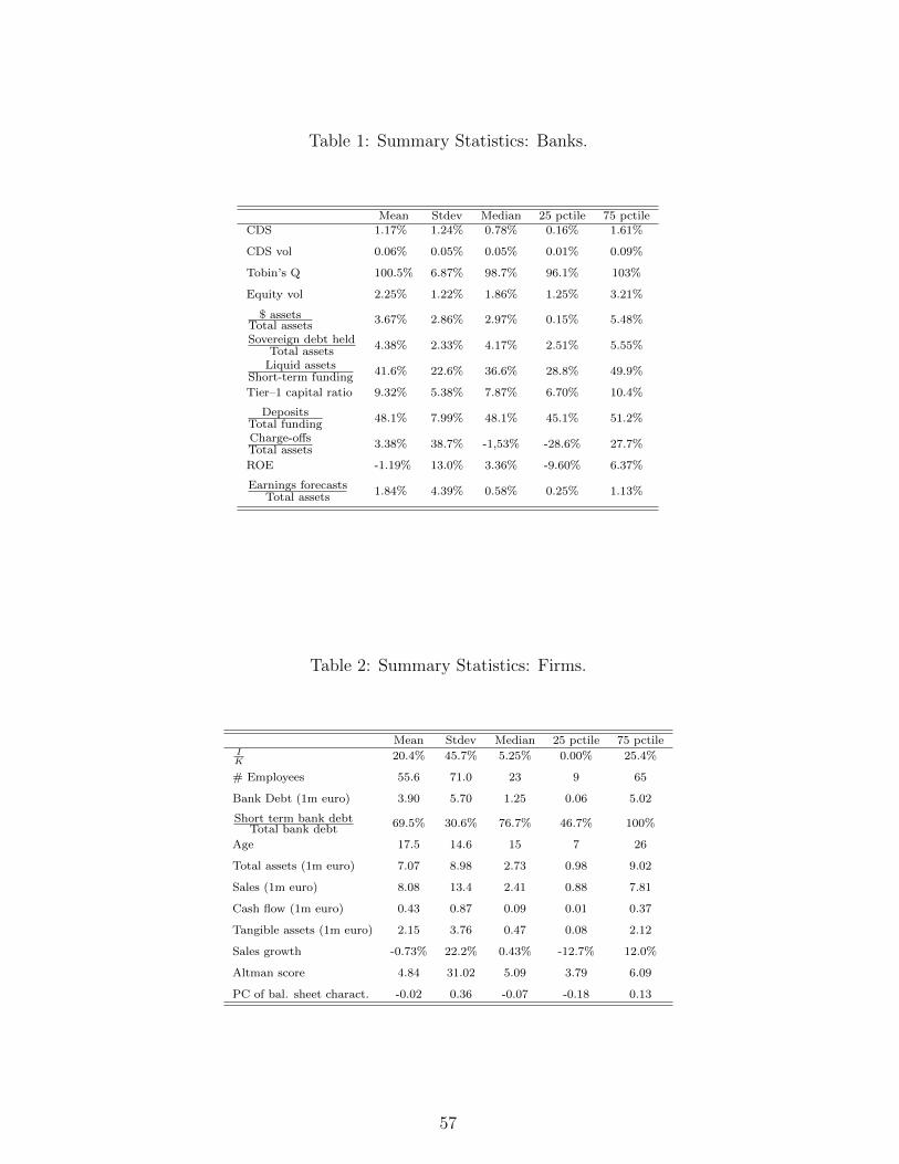
Table 1: Summary Statistics: Banks.

Mean Stdev Median 25 pctile 75 pctileCDS 1.17% 1.24% 0.78% 0.16% 1.61%

CDS vol 0.06% 0.05% 0.05% 0.01% 0.09%

Tobin’s Q 100.5% 6.87% 98.7% 96.1% 103%

Equity vol 2.25% 1.22% 1.86% 1.25% 3.21%

$ assetsTotal assets

3.67% 2.86% 2.97% 0.15% 5.48%

Sovereign debt heldTotal assets

4.38% 2.33% 4.17% 2.51% 5.55%

Liquid assetsShort-term funding

41.6% 22.6% 36.6% 28.8% 49.9%

Tier–1 capital ratio 9.32% 5.38% 7.87% 6.70% 10.4%

DepositsTotal funding

48.1% 7.99% 48.1% 45.1% 51.2%

Charge-offsTotal assets

3.38% 38.7% -1,53% -28.6% 27.7%

ROE -1.19% 13.0% 3.36% -9.60% 6.37%

Earnings forecastsTotal assets

1.84% 4.39% 0.58% 0.25% 1.13%

Table 2: Summary Statistics: Firms.

Mean Stdev Median 25 pctile 75 pctileIK

20.4% 45.7% 5.25% 0.00% 25.4%

# Employees 55.6 71.0 23 9 65

Bank Debt (1m euro) 3.90 5.70 1.25 0.06 5.02

Short term bank debtTotal bank debt

69.5% 30.6% 76.7% 46.7% 100%

Age 17.5 14.6 15 7 26

Total assets (1m euro) 7.07 8.98 2.73 0.98 9.02

Sales (1m euro) 8.08 13.4 2.41 0.88 7.81

Cash flow (1m euro) 0.43 0.87 0.09 0.01 0.37

Tangible assets (1m euro) 2.15 3.76 0.47 0.08 2.12

Sales growth -0.73% 22.2% 0.43% -12.7% 12.0%

Altman score 4.84 31.02 5.09 3.79 6.09

PC of bal. sheet charact. -0.02 0.36 -0.07 -0.18 0.13

57

Table 3: Banking Relationships.

Type of banking relationshipSingle Double Multiple

Age - Q1 81.8% 17.4% 0.80%

Age - Q2 79.3% 19.1% 1.60%

Age - Q3 77.5% 20.3% 2.20%

Age - Q4 76.7% 19.8% 3.50%

Size - Q1 83.1% 16.2% 0.70%

Size - Q2 73.4% 24.4% 2.20%

Size - Q3 70.2% 26.7% 3.10%

Size - Q4 65.5% 26.3% 8.20%

Total 78.9% 19.2% 1.90%

Notes: Percentage of firms with one, two, or multiple banking relationships, for different age and size quartiles.

58

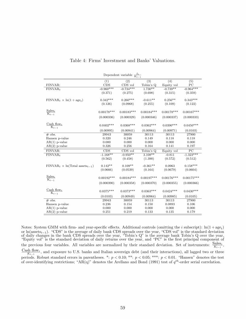
Table 4: Firms’ Investment and Banks’ Valuations.

Dependent variable ItKt−1

(1) (2) (3) (4) (5)FINVAR: CDS CDS vol Tobin’s Q Equity vol PCFINVARt -0.960*** -0.734*** 1.730** -0.739** -0.964***

(0.371) (0.275) (0.698) (0.315) (0.359)

FINVARt × ln(1 + aget) 0.342*** 0.260*** -0.611** 0.256** 0.343***(0.126) (0.0968) (0.255) (0.109) (0.122)

SalestKt−1

0.00178*** 0.00183*** 0.00184*** 0.00178*** 0.00167***

(0.000336) (0.000329) (0.000346) (0.000337) (0.000333)

Cash flowt

Kt−10.0402*** 0.0368*** 0.0362*** 0.0390*** 0.0450***

(0.00995) (0.00941) (0.00964) (0.00971) (0.0103)# obs. 29943 30059 30113 30113 27900Hansen p-value 0.320 0.246 0.149 0.118 0.118AR(1) p-value 0.000 0.000 0.000 0.000 0.000AR(2) p-value 0.326 0.256 0.164 0.141 0.197

FINVAR: CDS CDS vol Tobin’s Q Equity vol PCFINVARt -1.168** -0.950** 3.108** -0.811 -1.323***

(0.562) (0.458) (1.390) (0.572) (0.512)

FINVARt × ln(Total assetst−1) 0.142** 0.109** -0.361** 0.0963 0.158***(0.0666) (0.0539) (0.164) (0.0679) (0.0604)

SalestKt−1

0.00192*** 0.00184*** 0.00197*** 0.00176*** 0.00175***

(0.000390) (0.000358) (0.000370) (0.000355) (0.000366)

Cash flowt

Kt−10.0375*** 0.0373*** 0.0363*** 0.0424*** 0.0430***

(0.0103) (0.00949) (0.00964) (0.00985) (0.0105)# obs. 29943 30059 30113 30113 27900Hansen p-value 0.236 0.154 0.150 0.0893 0.106AR(1) p-value 0.000 0.000 0.000 0.000 0.000AR(2) p-value 0.251 0.219 0.133 0.135 0.179

Notes: System GMM with firm- and year-specific effects. Additional controls (omitting the i subscript): ln(1 + aget)or ln(assetst−1). “CDS” is the average of daily bank CDS spreads over the year, “CDS vol” is the standard deviationof daily changes in the bank CDS spreads over the year, “Tobin’s Q” is the average bank Tobin’s Q over the year,“Equity vol” is the standard deviation of daily returns over the year, and “PC” is the first principal component of

the previous four variables. All variables are normalized by their standard deviation. Set of instruments: Salest

Kt−1,

Cash flowt

Kt−1, and exposure to U.S. banks and Italian sovereign debt (and their interactions), all lagged two or three

periods. Robust standard errors in parentheses. *: p < 0.10; **: p < 0.05; ***: p < 0.01. “Hansen” denotes the testof over-identifying restrictions; “AR(q)” denotes the Arellano and Bond (1991) test of qth-order serial correlation.

59

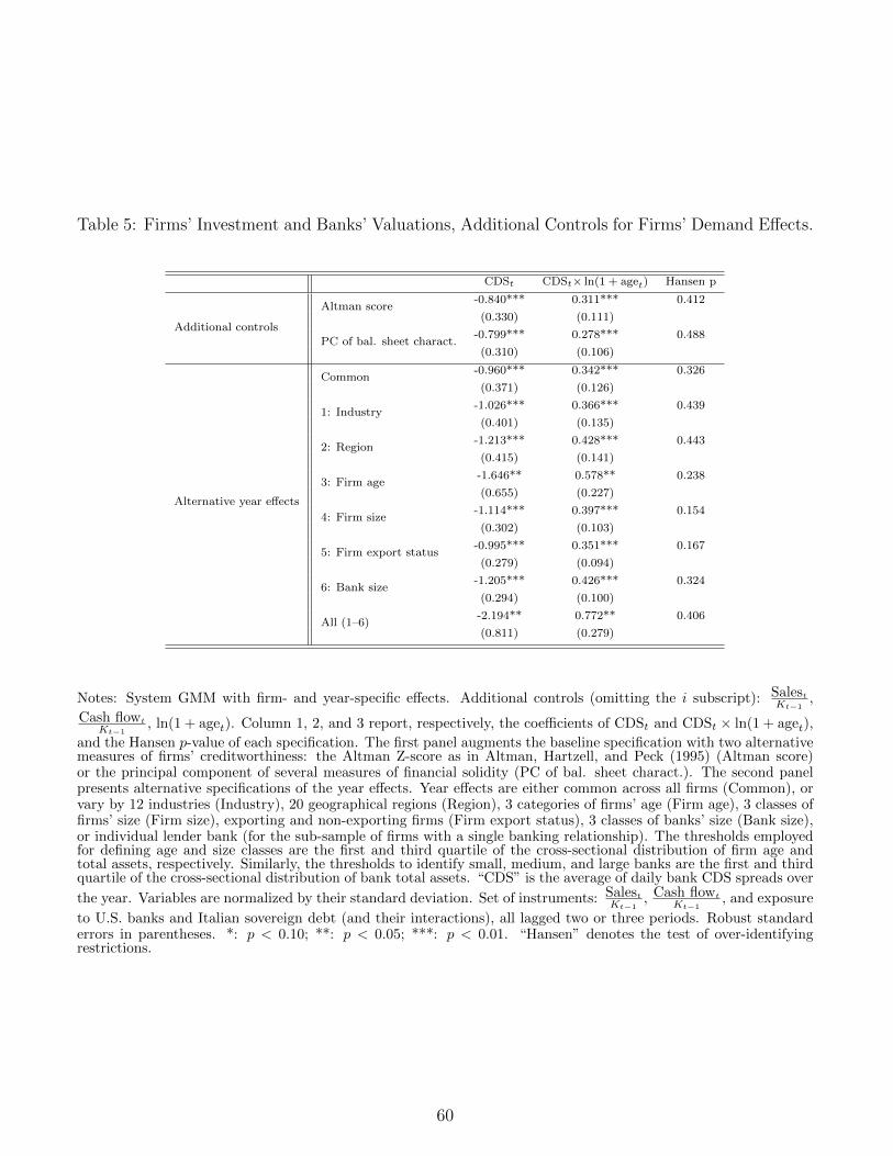
Table 5: Firms’ Investment and Banks’ Valuations, Additional Controls for Firms’ Demand Effects.

CDSt CDSt× ln(1 + aget) Hansen p

Additional controls

Altman score-0.840*** 0.311*** 0.412

(0.330) (0.111)

PC of bal. sheet charact.-0.799*** 0.278*** 0.488

(0.310) (0.106)

Alternative year effects

Common-0.960*** 0.342*** 0.326

(0.371) (0.126)

1: Industry-1.026*** 0.366*** 0.439

(0.401) (0.135)

2: Region-1.213*** 0.428*** 0.443

(0.415) (0.141)

3: Firm age-1.646** 0.578** 0.238

(0.655) (0.227)

4: Firm size-1.114*** 0.397*** 0.154

(0.302) (0.103)

5: Firm export status-0.995*** 0.351*** 0.167

(0.279) (0.094)

6: Bank size-1.205*** 0.426*** 0.324

(0.294) (0.100)

All (1–6)-2.194** 0.772** 0.406

(0.811) (0.279)

Notes: System GMM with firm- and year-specific effects. Additional controls (omitting the i subscript): Salest

Kt−1,

Cash flowt

Kt−1, ln(1 + aget). Column 1, 2, and 3 report, respectively, the coefficients of CDSt and CDSt × ln(1 + aget),

and the Hansen p-value of each specification. The first panel augments the baseline specification with two alternativemeasures of firms’ creditworthiness: the Altman Z-score as in Altman, Hartzell, and Peck (1995) (Altman score)or the principal component of several measures of financial solidity (PC of bal. sheet charact.). The second panelpresents alternative specifications of the year effects. Year effects are either common across all firms (Common), orvary by 12 industries (Industry), 20 geographical regions (Region), 3 categories of firms’ age (Firm age), 3 classes offirms’ size (Firm size), exporting and non-exporting firms (Firm export status), 3 classes of banks’ size (Bank size),or individual lender bank (for the sub-sample of firms with a single banking relationship). The thresholds employedfor defining age and size classes are the first and third quartile of the cross-sectional distribution of firm age andtotal assets, respectively. Similarly, the thresholds to identify small, medium, and large banks are the first and thirdquartile of the cross-sectional distribution of bank total assets. “CDS” is the average of daily bank CDS spreads over

the year. Variables are normalized by their standard deviation. Set of instruments: Salest

Kt−1, Cash flowt

Kt−1, and exposure

to U.S. banks and Italian sovereign debt (and their interactions), all lagged two or three periods. Robust standarderrors in parentheses. *: p < 0.10; **: p < 0.05; ***: p < 0.01. “Hansen” denotes the test of over-identifyingrestrictions.

60

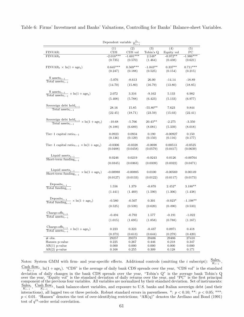
Table 6: Firms’ Investment and Banks’ Valuations, Controlling for Banks’ Balance-sheet Variables.

Dependent variable ItKt−1

(1) (2) (3) (4) (5)FINVAR: CDS CDS vol Tobin’s Q Equity vol PCFINVARt -2.018*** -1.601*** 2.548* -0.972** -1.986***

(0.735) (0.570) (1.464) (0.438) (0.621)

FINVARt × ln(1 + aget) 0.645*** 0.569*** -1.043** 0.337** 0.711***(0.247) (0.188) (0.525) (0.154) (0.215)

$ assetst−1

Total assetst−1-5.076 -8.613 26.00 -14.14 -18.89

(14.70) (15.80) (16.79) (13.80) (18.85)

$ assetst−1

Total assetst−1× ln(1 + aget) 2.072 3.316 -9.162 5.133 6.982

(5.408) (5.788) (6.423) (5.133) (6.977)

Sovereign debt heldt−1

Total assetst−128.16 15.85 -55.80** 7.623 9.844

(22.45) (18.71) (23.59) (15.03) (22.41)

Sovereign debt heldt−1

Total assetst−1× ln(1 + aget) -10.68 -5.766 20.43** -2.275 -3.350

(8.188) (6.689) (8.081) (5.339) (8.018)

Tier–1 capital ratiot−1 0.0923 0.0934 0.190 -0.00927 0.150(0.136) (0.129) (0.150) (0.116) (0.177)

Tier–1 capital ratiot−1 × ln(1 + aget) -0.0306 -0.0328 -0.0698 0.00513 -0.0525(0.0488) (0.0458) (0.0579) (0.0417) (0.0639)

Liquid assetst−1

Short-term fundingt−10.0246 0.0219 -0.0243 0.0126 -0.00764

(0.0345) (0.0363) (0.0339) (0.0322) (0.0471)

Liquid assetst−1

Short-term fundingt−1× ln(1 + aget) -0.00988 -0.00885 0.0100 -0.00569 0.00149

(0.0127) (0.0133) (0.0122) (0.0117) (0.0173)

Depositst−1

Total fundingt−11.556 1.379 -0.870 2.452* 3.188**

(1.441) (1.469) (1.590) (1.306) (1.438)

Depositst−1

Total fundingt−1× ln(1 + aget) -0.580 -0.507 0.301 -0.923* -1.198**

(0.525) (0.539) (0.620) (0.490) (0.533)

Charge-offst−1

Total assetst−1-0.494 -0.792 1.577 -0.191 -1.022

(1.015) (1.695) (1.858) (0.788) (1.167)

Charge-offst−1

Total assetst−1× ln(1 + aget) 0.223 0.323 -0.437 0.0971 0.418

(0.373) (0.613) (0.644) (0.278) (0.420)# obs. 29257 29373 29486 29486 27410Hansen p-value 0.225 0.267 0.446 0.218 0.347AR(1) p-value 0.000 0.000 0.000 0.000 0.000AR(2) p-value 0.168 0.255 0.309 0.128 0.171

Notes: System GMM with firm- and year-specific effects. Additional controls (omitting the i subscript): Salest

Kt−1,

Cash flowt

Kt−1, ln(1 + aget). “CDS” is the average of daily bank CDS spreads over the year, “CDS vol” is the standard

deviation of daily changes in the bank CDS spreads over the year, “Tobin’s Q” is the average bank Tobin’s Qover the year, “Equity vol” is the standard deviation of daily returns over the year, and “PC” is the first principalcomponent of the previous four variables. All variables are normalized by their standard deviation. Set of instruments:Salest

Kt−1, Cash flowt

Kt−1, bank balance-sheet variables, and exposure to U.S. banks and Italian sovereign debt (and their

interactions), all lagged two or three periods. Robust standard errors in parentheses. *: p < 0.10; **: p < 0.05; ***:p < 0.01. “Hansen” denotes the test of over-identifying restrictions; “AR(q)” denotes the Arellano and Bond (1991)test of qth-order serial correlation.

61

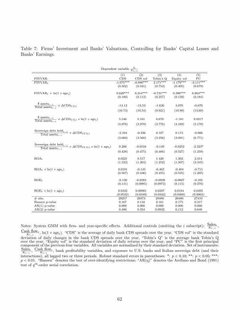
Table 7: Firms’ Investment and Banks’ Valuations, Controlling for Banks’ Capital Losses andBanks’ Earnings.

Dependent variable ItKt−1

(1) (2) (3) (4) (5)FINVAR: CDS CDS vol Tobin’s Q Equity vol PCFINVARt -1.675*** -0.886*** 2.171*** -1.179*** -3.111***

(0.502) (0.341) (0.753) (0.405) (0.679)

FINVARt × ln(1 + aget) 0.629*** 0.314*** -0.731*** 0.396*** 0.864***(0.180) (0.112) (0.257) (0.139) (0.184)

$ assetst−1

Total assetst−1×∆CDSUS,t -14.13 -13.53 -1.626 4.070 -0.676

(10.73) (10.54) (9.921) (10.99) (13.60)

$ assetst−1

Total assetst−1×∆CDSUS,t × ln(1 + aget) 5.546 5.101 0.670 -1.181 0.0317

(4.076) (3.978) (3.776) (4.169) (5.170)

Sovereign debt heldt−1

Total assetst−1×∆CDSITA,t -2.164 -0.336 0.167 0.115 -0.666

(3.060) (3.560) (3.256) (3.091) (6.771)

Sovereign debt heldt−1

Total assetst−1×∆CDSITA,t × ln(1 + aget) 0.200 -0.0534 -0.149 -0.0252 -2.323*

(0.428) (0.475) (0.466) (0.527) (1.259)

ROAt 0.0221 0.517 1.420 1.302 2.314(1.523) (1.204) (1.252) (1.507) (3.345)

ROAt × ln(1 + aget) 0.0191 -0.145 -0.462 -0.404 -0.715(0.567) (0.436) (0.455) (0.535) (1.205)

ROEt -0.120 -0.0383 -0.0939 -0.0607 -0.165(0.141) (0.0985) (0.0972) (0.115) (0.270)

ROEt × ln(1 + aget) 0.0432 0.00981 0.0297 0.0184 0.0495(0.0532) (0.0349) (0.0342) (0.0400) (0.0964)

# obs. 29257 29373 29486 29486 27410Hansen p-value 0.167 0.134 0.161 0.175 0.317AR(1) p-value 0.000 0.000 0.000 0.000 0.000AR(2) p-value 0.486 0.354 0.0932 0.112 0.640

Notes: System GMM with firm- and year-specific effects. Additional controls (omitting the i subscript): Salest

Kt−1,

Cash flowt

Kt−1, ln(1 + aget). “CDS” is the average of daily bank CDS spreads over the year, “CDS vol” is the standard

deviation of daily changes in the bank CDS spreads over the year, “Tobin’s Q” is the average bank Tobin’s Qover the year, “Equity vol” is the standard deviation of daily returns over the year, and “PC” is the first principalcomponent of the previous four variables. All variables are normalized by their standard deviation. Set of instruments:Salest

Kt−1, Cash flowt

Kt−1, bank profitability variables, and exposure to U.S. banks and Italian sovereign debt (and their

interactions), all lagged two or three periods. Robust standard errors in parentheses. *: p < 0.10; **: p < 0.05; ***:p < 0.01. “Hansen” denotes the test of over-identifying restrictions; “AR(q)” denotes the Arellano and Bond (1991)test of qth-order serial correlation.

62

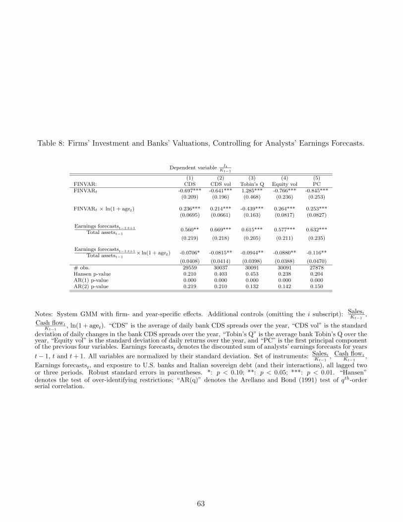
Table 8: Firms’ Investment and Banks’ Valuations, Controlling for Analysts’ Earnings Forecasts.

Dependent variable ItKt−1

(1) (2) (3) (4) (5)FINVAR: CDS CDS vol Tobin’s Q Equity vol PCFINVARt -0.697*** -0.641*** 1.285*** -0.766*** -0.845***

(0.209) (0.196) (0.468) (0.236) (0.253)

FINVARt × ln(1 + aget) 0.236*** 0.214*** -0.439*** 0.264*** 0.253***(0.0695) (0.0661) (0.163) (0.0817) (0.0827)

Earnings forecastst−1:t+1

Total assetst−10.560** 0.669*** 0.615*** 0.577*** 0.632***

(0.219) (0.218) (0.205) (0.211) (0.235)

Earnings forecastst−1:t+1

Total assetst−1× ln(1 + aget) -0.0706* -0.0815** -0.0944** -0.0880** -0.116**

(0.0408) (0.0414) (0.0398) (0.0388) (0.0470)# obs. 29559 30037 30091 30091 27878Hansen p-value 0.210 0.403 0.453 0.238 0.204AR(1) p-value 0.000 0.000 0.000 0.000 0.000AR(2) p-value 0.219 0.210 0.132 0.142 0.150

Notes: System GMM with firm- and year-specific effects. Additional controls (omitting the i subscript): Salest

Kt−1,

Cash flowt

Kt−1, ln(1 + aget). “CDS” is the average of daily bank CDS spreads over the year, “CDS vol” is the standard

deviation of daily changes in the bank CDS spreads over the year, “Tobin’s Q” is the average bank Tobin’s Q over theyear, “Equity vol” is the standard deviation of daily returns over the year, and “PC” is the first principal componentof the previous four variables. Earnings forecastst denotes the discounted sum of analysts’ earnings forecasts for years

t− 1, t and t+ 1. All variables are normalized by their standard deviation. Set of instruments: Salest

Kt−1, Cash flowt

Kt−1,

Earnings forecastst, and exposure to U.S. banks and Italian sovereign debt (and their interactions), all lagged twoor three periods. Robust standard errors in parentheses. *: p < 0.10; **: p < 0.05; ***: p < 0.01. “Hansen”denotes the test of over-identifying restrictions; “AR(q)” denotes the Arellano and Bond (1991) test of qth-orderserial correlation.

63

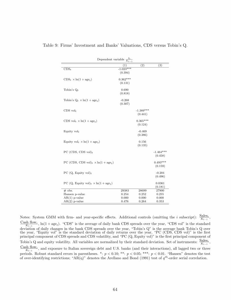
Table 9: Firms’ Investment and Banks’ Valuations, CDS versus Tobin’s Q.

Dependent variable ItKt−1

(1) (2) (3)CDSt -1.023***

(0.394)

CDSt × ln(1 + aget) 0.362***(0.131)

Tobin’s Qt 0.690(0.818)

Tobin’s Qt × ln(1 + aget) -0.268(0.307)

CDS volt -1.389***(0.441)

CDS volt × ln(1 + aget) 0.365***(0.124)

Equity volt -0.469(0.386)

Equity volt × ln(1 + aget) 0.156(0.135)

PC (CDS, CDS vol)t -1.464***(0.458)

PC (CDS, CDS vol)t × ln(1 + aget) 0.493***(0.159)

PC (Q, Equity vol)t -0.204(0.496)

PC (Q, Equity vol)t × ln(1 + aget) 0.0361(0.181)

# obs. 29383 28699 27900Hansen p-value 0.254 0.252 0.255AR(1) p-value 0.000 0.000 0.000AR(2) p-value 0.476 0.264 0.353

Notes: System GMM with firm- and year-specific effects. Additional controls (omitting the i subscript): Salest

Kt−1,

Cash flowt

Kt−1, ln(1 + aget). “CDS” is the average of daily bank CDS spreads over the year, “CDS vol” is the standard

deviation of daily changes in the bank CDS spreads over the year, “Tobin’s Q” is the average bank Tobin’s Q overthe year, “Equity vol” is the standard deviation of daily returns over the year, “PC (CDS, CDS vol)” is the firstprincipal component of CDS spreads and CDS volatility, and “PC (Q, Equity vol)” is the first principal component of

Tobin’s Q and equity volatility. All variables are normalized by their standard deviation. Set of instruments: Salest

Kt−1,

Cash flowt

Kt−1, and exposure to Italian sovereign debt and U.S. banks (and their interactions), all lagged two or three

periods. Robust standard errors in parentheses. *: p < 0.10; **: p < 0.05; ***: p < 0.01. “Hansen” denotes the testof over-identifying restrictions; “AR(q)” denotes the Arellano and Bond (1991) test of qth-order serial correlation.

64

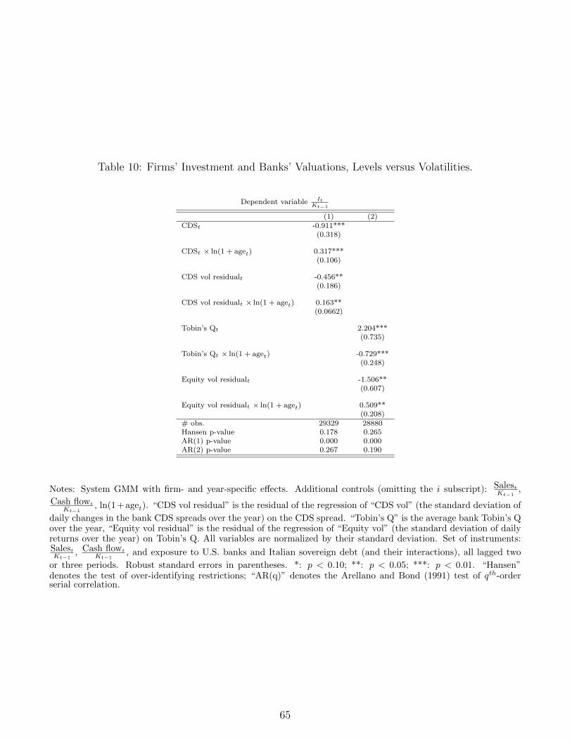
Table 10: Firms’ Investment and Banks’ Valuations, Levels versus Volatilities.

Dependent variable ItKt−1

(1) (2)CDSt -0.911***

(0.318)

CDSt × ln(1 + aget) 0.317***(0.106)

CDS vol residualt -0.456**(0.186)

CDS vol residualt × ln(1 + aget) 0.163**(0.0662)

Tobin’s Qt 2.204***(0.735)

Tobin’s Qt × ln(1 + aget) -0.729***(0.248)

Equity vol residualt -1.506**(0.607)

Equity vol residualt × ln(1 + aget) 0.509**(0.208)

# obs. 29329 28880Hansen p-value 0.178 0.265AR(1) p-value 0.000 0.000AR(2) p-value 0.267 0.190

Notes: System GMM with firm- and year-specific effects. Additional controls (omitting the i subscript): Salest

Kt−1,

Cash flowt

Kt−1, ln(1+aget). “CDS vol residual” is the residual of the regression of “CDS vol” (the standard deviation of

daily changes in the bank CDS spreads over the year) on the CDS spread. “Tobin’s Q” is the average bank Tobin’s Qover the year, “Equity vol residual” is the residual of the regression of “Equity vol” (the standard deviation of dailyreturns over the year) on Tobin’s Q. All variables are normalized by their standard deviation. Set of instruments:Salest

Kt−1, Cash flowt

Kt−1, and exposure to U.S. banks and Italian sovereign debt (and their interactions), all lagged two

or three periods. Robust standard errors in parentheses. *: p < 0.10; **: p < 0.05; ***: p < 0.01. “Hansen”denotes the test of over-identifying restrictions; “AR(q)” denotes the Arellano and Bond (1991) test of qth-orderserial correlation.

65

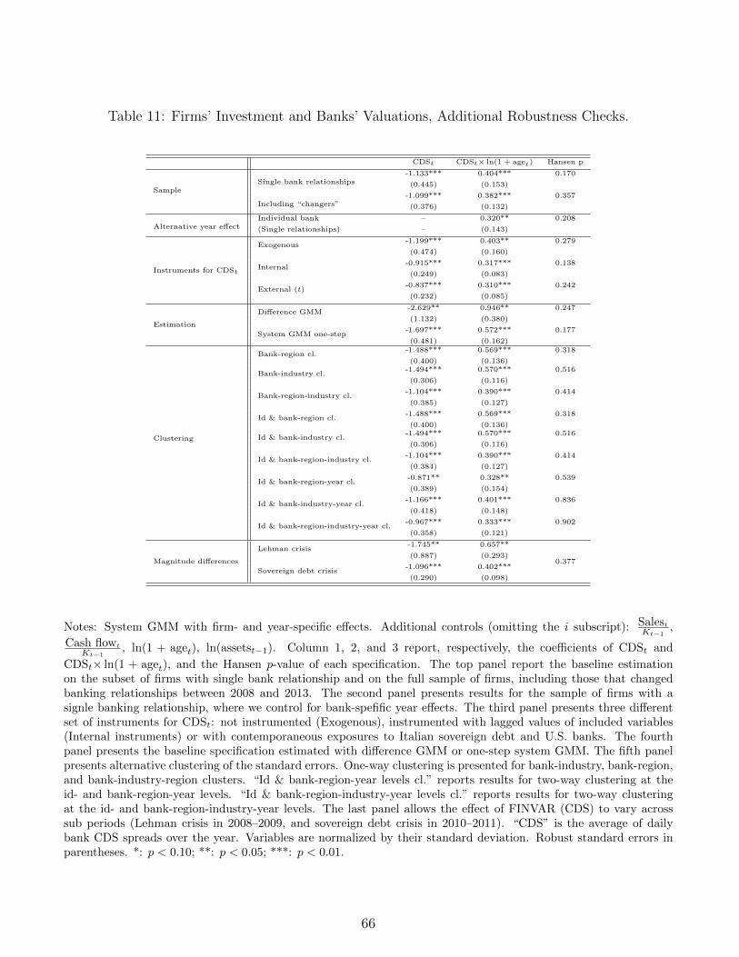
Table 11: Firms’ Investment and Banks’ Valuations, Additional Robustness Checks.

CDSt CDSt× ln(1 + aget) Hansen p

SampleSingle bank relationships

-1.133*** 0.404*** 0.170

(0.445) (0.153)

Including “changers”-1.099*** 0.382*** 0.357

(0.376) (0.132)

Alternative year effectIndividual bank – 0.320** 0.208

(Single relationships) – (0.143)

Instruments for CDSt

Exogenous-1.199*** 0.403** 0.279

(0.474) (0.160)

Internal-0.915*** 0.317*** 0.138

(0.249) (0.083)

External (t)-0.837*** 0.310*** 0.242

(0.232) (0.085)

Estimation

Difference GMM-2.629** 0.946** 0.247

(1.132) (0.380)

System GMM one-step-1.697*** 0.572*** 0.177

(0.481) (0.162)

Clustering

Bank-region cl.-1.488*** 0.569*** 0.318

(0.400) (0.136)

Bank-industry cl.-1.494*** 0.570*** 0.516

(0.306) (0.116)

Bank-region-industry cl.-1.104*** 0.390*** 0.414

(0.385) (0.127)

Id & bank-region cl.-1.488*** 0.569*** 0.318

(0.400) (0.136)

Id & bank-industry cl.-1.494*** 0.570*** 0.516

(0.306) (0.116)

Id & bank-region-industry cl.-1.104*** 0.390*** 0.414

(0.384) (0.127)

Id & bank-region-year cl.-0.871** 0.328** 0.539

(0.389) (0.154)

Id & bank-industry-year cl.-1.166*** 0.401*** 0.836

(0.418) (0.148)

Id & bank-region-industry-year cl.-0.967*** 0.333*** 0.902

(0.358) (0.121)

Magnitude differences

Lehman crisis-1.745** 0.657**

0.377(0.887) (0.293)

Sovereign debt crisis-1.096*** 0.402***

(0.290) (0.098)

Notes: System GMM with firm- and year-specific effects. Additional controls (omitting the i subscript): Salest

Kt−1,

Cash flowt

Kt−1, ln(1 + aget), ln(assetst−1). Column 1, 2, and 3 report, respectively, the coefficients of CDSt and

CDSt× ln(1 + aget), and the Hansen p-value of each specification. The top panel report the baseline estimationon the subset of firms with single bank relationship and on the full sample of firms, including those that changedbanking relationships between 2008 and 2013. The second panel presents results for the sample of firms with asignle banking relationship, where we control for bank-spefific year effects. The third panel presents three differentset of instruments for CDSt: not instrumented (Exogenous), instrumented with lagged values of included variables(Internal instruments) or with contemporaneous exposures to Italian sovereign debt and U.S. banks. The fourthpanel presents the baseline specification estimated with difference GMM or one-step system GMM. The fifth panelpresents alternative clustering of the standard errors. One-way clustering is presented for bank-industry, bank-region,and bank-industry-region clusters. “Id & bank-region-year levels cl.” reports results for two-way clustering at theid- and bank-region-year levels. “Id & bank-region-industry-year levels cl.” reports results for two-way clusteringat the id- and bank-region-industry-year levels. The last panel allows the effect of FINVAR (CDS) to vary acrosssub periods (Lehman crisis in 2008–2009, and sovereign debt crisis in 2010–2011). “CDS” is the average of dailybank CDS spreads over the year. Variables are normalized by their standard deviation. Robust standard errors inparentheses. *: p < 0.10; **: p < 0.05; ***: p < 0.01.

66

Table 12: Firms’ Investment and Banks’ Valuations, Interaction Effects by Age Terciles.

(1)

Dependent variable: ItKt−1

CDSt × youngt -0.405***(0.155)

CDSt × middle agedt -0.0130(0.0998)

CDSt × oldt 0.298**(0.146)

# obs. 29943Hansen p-value 0.219AR(1) p-value 0.000AR(2) p-value 0.405

Notes: System GMM with firm- and year-specific effects. Additional controls (omitting the i subscript): Salest

Kt−1,

Cash flowt

Kt−1, ln(1 + aget). “CDS” is the average of daily bank CDS spreads over the year. “young” “middle aged”,

and “old” are dummy variables identifying the terciles of the firm age distribution. All variables are normalized by

their standard deviation. Set of instruments: Salest

Kt−1, Cash flowt

Kt−1, and exposure to U.S. banks and Italian sovereign

debt (and their interactions), all lagged two or three periods. Robust standard errors in parentheses. *: p < 0.10; **:p < 0.05; ***: p < 0.01. “Hansen” denotes the test of over-identifying restrictions; “AR(q)” denotes the Arellanoand Bond (1991) test of qth-order serial correlation.

67

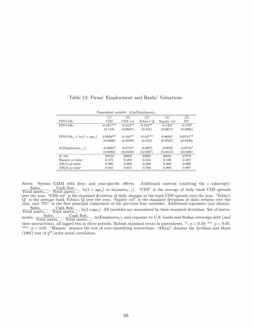
Table 13: Firms’ Employment and Banks’ Valuations.

Dependent variable: ∆ ln(Employees)t

(1) (2) (3) (4) (5)FINVAR: CDS CDS vol Tobin’s Q Equity vol PCFINVARt -0.381*** -0.212** 0.724** -0.135* -0.170*

(0.118) (0.0947) (0.345) (0.0817) (0.0906)

FINVARt × ln(1 + aget) 0.0958** 0.102** -0.447** 0.0858* 0.0745**(0.0400) (0.0506) (0.213) (0.0507) (0.0340)

ln(Employeest−1) -0.0692* -0.0741* -0.0675 -0.0632 -0.0754*(0.0386) (0.0448) (0.0507) (0.0413) (0.0406)

# obs. 29559 30037 30091 30091 27878Hansen p-value 0.575 0.203 0.224 0.196 0.287AR(1) p-value 0.000 0.000 0.000 0.000 0.000AR(2) p-value 0.941 0.837 0.780 0.998 0.997

Notes: System GMM with firm- and year-specific effects. Additional controls (omitting the i subscript):Salest

Total assetst−1, Cash flowt

Total assetst−1, ln(1 + aget) or ln(assetst−1). “CDS” is the average of daily bank CDS spreads

over the year, “CDS vol” is the standard deviation of daily changes in the bank CDS spreads over the year, “Tobin’sQ” is the average bank Tobin’s Q over the year, “Equity vol” is the standard deviation of daily returns over theyear, and “PC” is the first principal component of the previous four variables. Additional regressors (not shown):

Salest

Total assetst−1, Cash flowt

Total assetst−1, ln(1+aget). All variables are normalized by their standard deviation. Set of instru-

ments: Salest

Total assetst−1, Cash flowt

Total assetst−1, ln(Employeest), and exposure to U.S. banks and Italian sovereign debt (and

their interactions), all lagged two or three periods. Robust standard errors in parentheses. *: p < 0.10; **: p < 0.05;***: p < 0.01. “Hansen” denotes the test of over-identifying restrictions; “AR(q)” denotes the Arellano and Bond(1991) test of qth-order serial correlation.

68

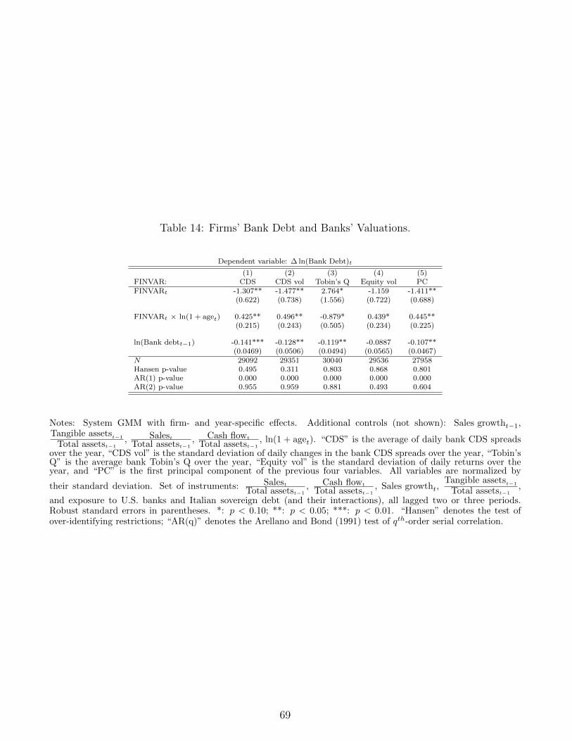
Table 14: Firms’ Bank Debt and Banks’ Valuations.

Dependent variable: ∆ ln(Bank Debt)t

(1) (2) (3) (4) (5)FINVAR: CDS CDS vol Tobin’s Q Equity vol PCFINVARt -1.307** -1.477** 2.764* -1.159 -1.411**

(0.622) (0.738) (1.556) (0.722) (0.688)

FINVARt × ln(1 + aget) 0.425** 0.496** -0.879* 0.439* 0.445**(0.215) (0.243) (0.505) (0.234) (0.225)

ln(Bank debtt−1) -0.141*** -0.128** -0.119** -0.0887 -0.107**(0.0469) (0.0506) (0.0494) (0.0565) (0.0467)

N 29092 29351 30040 29536 27958Hansen p-value 0.495 0.311 0.803 0.868 0.801AR(1) p-value 0.000 0.000 0.000 0.000 0.000AR(2) p-value 0.955 0.959 0.881 0.493 0.604

Notes: System GMM with firm- and year-specific effects. Additional controls (not shown): Sales growtht−1,Tangible assetst−1

Total assetst−1, Salest

Total assetst−1, Cash flowt

Total assetst−1, ln(1 + aget). “CDS” is the average of daily bank CDS spreads

over the year, “CDS vol” is the standard deviation of daily changes in the bank CDS spreads over the year, “Tobin’sQ” is the average bank Tobin’s Q over the year, “Equity vol” is the standard deviation of daily returns over theyear, and “PC” is the first principal component of the previous four variables. All variables are normalized by

their standard deviation. Set of instruments: Salest

Total assetst−1, Cash flowt

Total assetst−1, Sales growtht,

Tangible assetst−1

Total assetst−1,

and exposure to U.S. banks and Italian sovereign debt (and their interactions), all lagged two or three periods.Robust standard errors in parentheses. *: p < 0.10; **: p < 0.05; ***: p < 0.01. “Hansen” denotes the test ofover-identifying restrictions; “AR(q)” denotes the Arellano and Bond (1991) test of qth-order serial correlation.

69

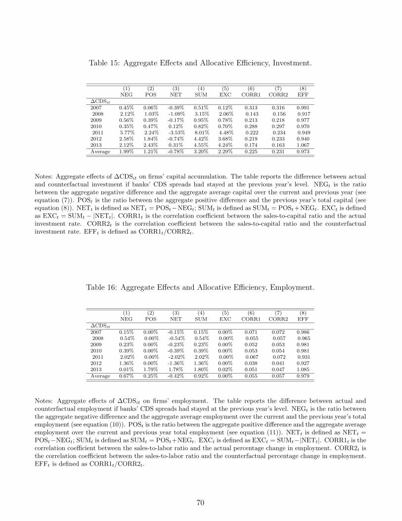
Table 15: Aggregate Effects and Allocative Efficiency, Investment.

(1) (2) (3) (4) (5) (6) (7) (8)NEG POS NET SUM EXC CORR1 CORR2 EFF

∆CDSit

2007 0.45% 0.06% -0.39% 0.51% 0.12% 0.313 0.316 0.9912008 2.12% 1.03% -1.09% 3.15% 2.06% 0.143 0.156 0.917

2009 0.56% 0.39% -0.17% 0.95% 0.78% 0.213 0.218 0.9772010 0.35% 0.47% 0.12% 0.82% 0.70% 0.288 0.297 0.9702011 5.77% 2.24% -3.53% 8.01% 4.48% 0.222 0.234 0.949

2012 2.58% 1.84% -0.74% 4.42% 3.68% 0.219 0.233 0.9402013 2.12% 2.43% 0.31% 4.55% 4.24% 0.174 0.163 1.067Average 1.99% 1.21% -0.78% 3.20% 2.29% 0.225 0.231 0.973

Notes: Aggregate effects of ∆CDSit on firms’ capital accumulation. The table reports the difference between actualand counterfactual investment if banks’ CDS spreads had stayed at the previous year’s level. NEGt is the ratiobetween the aggregate negative difference and the aggregate average capital over the current and previous year (seeequation (7)). POSt is the ratio between the aggregate positive difference and the previous year’s total capital (seeequation (8)). NETt is defined as NETt = POSt−NEGt; SUMt is defined as SUMt = POSt+NEGt. EXCt is definedas EXCt = SUMt − |NETt|. CORR1t is the correlation coefficient between the sales-to-capital ratio and the actualinvestment rate. CORR2t is the correlation coefficient between the sales-to-capital ratio and the counterfactualinvestment rate. EFFt is defined as CORR1t/CORR2t.

Table 16: Aggregate Effects and Allocative Efficiency, Employment.

(1) (2) (3) (4) (5) (6) (7) (8)NEG POS NET SUM EXC CORR1 CORR2 EFF

∆CDSit

2007 0.15% 0.00% -0.15% 0.15% 0.00% 0.071 0.072 0.9862008 0.54% 0.00% -0.54% 0.54% 0.00% 0.055 0.057 0.965

2009 0.23% 0.00% -0.23% 0.23% 0.00% 0.052 0.053 0.9812010 0.39% 0.00% -0.39% 0.39% 0.00% 0.053 0.054 0.9812011 2.02% 0.00% -2.02% 2.02% 0.00% 0.067 0.072 0.931

2012 1.36% 0.00% -1.36% 1.36% 0.00% 0.038 0.041 0.9272013 0.01% 1.79% 1.78% 1.80% 0.02% 0.051 0.047 1.085Average 0.67% 0.25% -0.42% 0.92% 0.00% 0.055 0.057 0.979

Notes: Aggregate effects of ∆CDSit on firms’ employment. The table reports the difference between actual andcounterfactual employment if banks’ CDS spreads had stayed at the previous year’s level. NEGt is the ratio betweenthe aggregate negative difference and the aggregate average employment over the current and the previous year’s totalemployment (see equation (10)). POSt is the ratio between the aggregate positive difference and the aggregate averageemployment over the current and previous year total employment (see equation (11)). NETt is defined as NETt =POSt−NEGt; SUMt is defined as SUMt = POSt+NEGt. EXCt is defined as EXCt = SUMt−|NETt|. CORR1t is thecorrelation coefficient between the sales-to-labor ratio and the actual percentage change in employment. CORR2t isthe correlation coefficient between the sales-to-labor ratio and the counterfactual percentage change in employment.EFFt is defined as CORR1t/CORR2t.

70

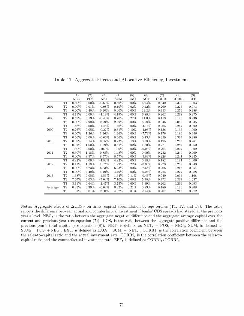
Table 17: Aggregate Effects and Allocative Efficiency, Investment.

(1) (2) (3) (4) (5) (6) (7) (8) (9)NEG POS NET SUM EXC ACT CORR1 CORR2 EFF

2007T1 0.60% 0.00% -0.60% 0.60% 0.00% 6.94% 0.340 0.339 1.003T2 0.09% 0.01% -0.08% 0.10% 0.02% 0.42% 0.269 0.276 0.973T3 0.00% 0.40% 0.40% 0.40% 0.00% 23.2% 0.253 0.256 0.988

2008T1 4.19% 0.00% -4.19% 4.19% 0.00% 6.88% 0.262 0.268 0.975T2 0.57% 0.13% -0.43% 0.70% 0.27% 11.0% 0.113 0.120 0.936T3 0.00% 2.99% 2.99% 2.99% 0.00% 6.58% 0.046 0.050 0.935

2009T1 1.46% 0.00% -1.46% 1.46% 0.00% -4.14% 0.265 0.267 0.992T2 0.26% 0.05% -0.22% 0.31% 0.10% -4.93% 0.136 0.136 1.000T3 0.00% 1.26% 1.26% 1.26% 0.00% -7.79% 0.176 0.186 0.946

2010T1 0.66% 0.00% -0.66% 0.66% 0.00% 0.13% 0.359 0.364 0.986T2 0.09% 0.14% 0.05% 0.23% 0.18% 0.08% 0.195 0.203 0.961T3 0.01% 1.60% 1.59% 0.61% 0.02% 1.80% 0.271 0.282 0.960

2011T1 10.0% 0.00% -10.0% 10.0% 0.00% -0.23% 0.204 0.202 1.009T2 0.30% 1.18% 0.88% 1.48% 0.60% 0.00% 0.232 0.240 0.969T3 0.00% 8.57% 8.57% 8.57% 0.00% -5.89% 0.228 0.241 0.945

2012T1 4.82% 0.00% -4.82% 4.82% 0.00% 0.38% 0.182 0.181 1.006T2 0.11% 1.18% 1.07% 1.29% 0.22% -0.38% 0.273 0.289 0.943T3 0.00% 6.23% 6.23% 6.23% 0.00% -2.58% 0.206 0.216 0.954

2013T1 0.00% 4.49% 4.49% 4.49% 0.00% -0.25% 0.225 0.227 0.988T2 1.58% 0.05% -1.53% 1.64% 0.11% -0.43% 0.040 0.035 1.168T3 7.07% 0.03% -7.04% 7.10% 0.06% 5.28% 0.272 0.262 1.037

AverageT1 3.11% 0.64% -2.47% 3.75% 0.00% 1.39% 0.262 0.264 0.993T2 0.43% 0.39% -0.04% 0.82% 0.21% 0.83% 0.180 0.186 0.968T3 1.01% 3.01% 2.00% 4.02% 0.01% 2.94% 0.207 0.213 0.972

Notes: Aggregate effects of ∆CDSit on firms’ capital accumulation by age terciles (T1, T2, and T3). The tablereports the difference between actual and counterfactual investment if banks’ CDS spreads had stayed at the previousyear’s level. NEGt is the ratio between the aggregate negative difference and the aggregate average capital over thecurrent and previous year (see equation (7)). POSt is the ratio between the aggregate positive difference and theprevious year’s total capital (see equation (8)). NETt is defined as NETt = POSt − NEGt; SUMt is defined asSUMt = POSt + NEGt. EXCt is defined as EXCt = SUMt − |NETt|. CORR1t is the correlation coefficient betweenthe sales-to-capital ratio and the actual investment rate. CORR2t is the correlation coefficient between the sales-to-capital ratio and the counterfactual investment rate. EFFt is defined as CORR1t/CORR2t.

71

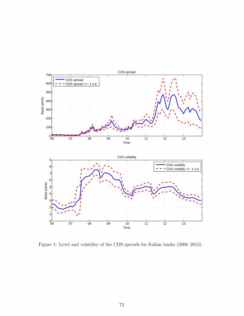
06 07 08 09 10 11 12 130

100

200

300

400

500

600

700

Time

Bas

is p

oint

s

CDS spread

06 07 08 09 10 11 12 130

1

2

3

4

5

6

7

8

9

Time

Bas

is p

oint

s

CDS volatility

CDS spreadCDS spread +/− 1 s.d.

CDS volatilityCDS volatility +/− 1 s.d.

Figure 1: Level and volatility of the CDS spreads for Italian banks (2006–2013).

72

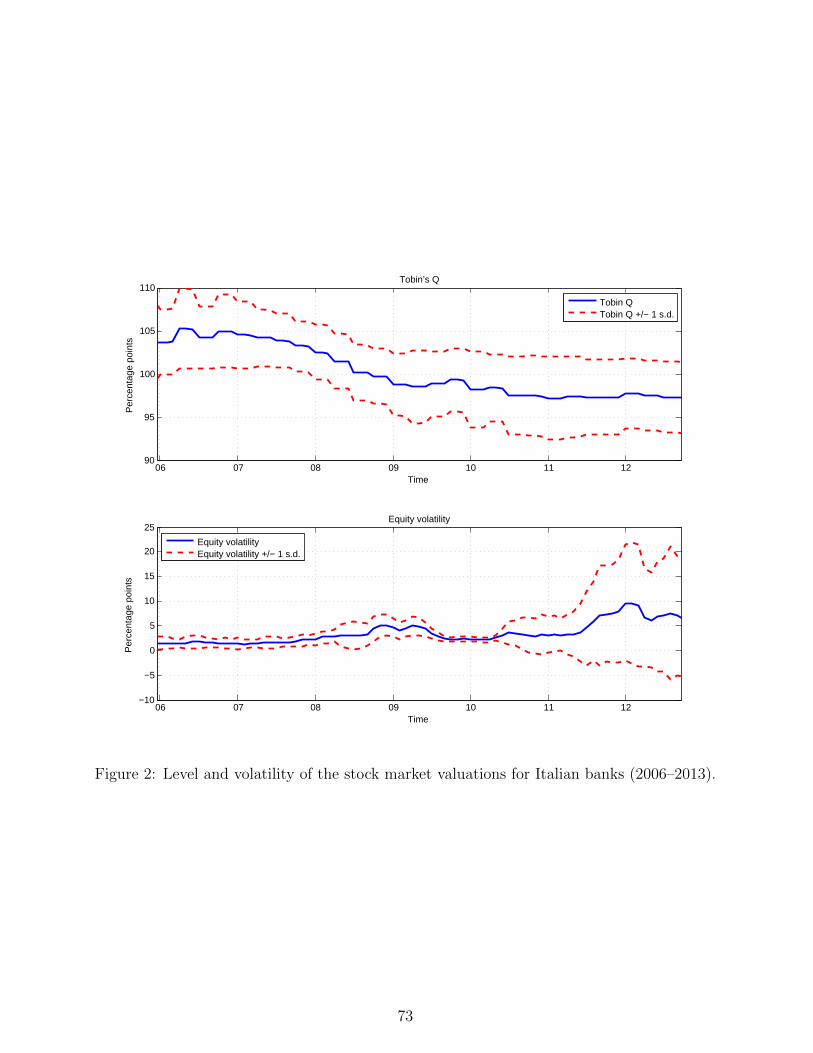
06 07 08 09 10 11 1290

95

100

105

110

Time

Per

cent

age

poin

ts

Tobin’s Q

06 07 08 09 10 11 12−10

−5

0

5

10

15

20

25

Time

Per

cent

age

poin

ts

Equity volatility

Tobin QTobin Q +/− 1 s.d.

Equity volatilityEquity volatility +/− 1 s.d.

Figure 2: Level and volatility of the stock market valuations for Italian banks (2006–2013).

73

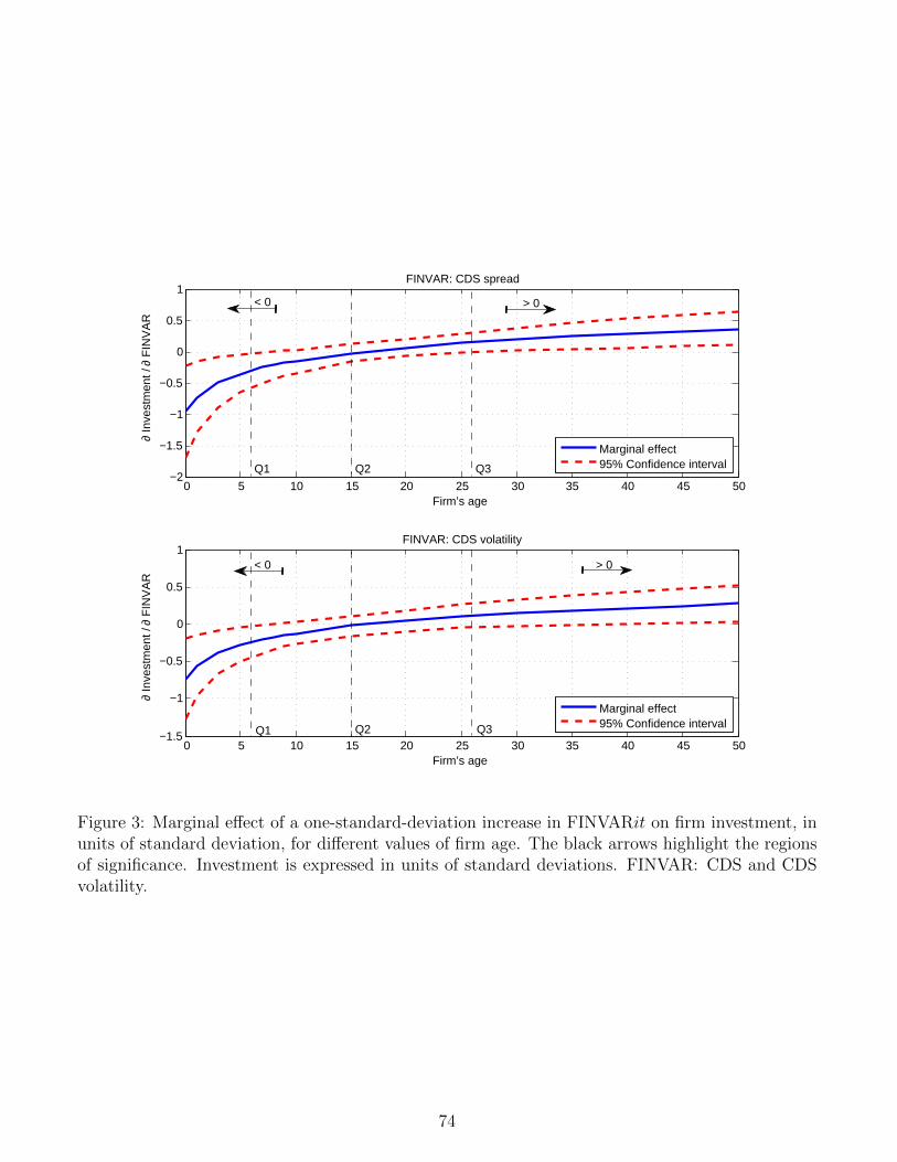
0 5 10 15 20 25 30 35 40 45 50−2

−1.5

−1

−0.5

0

0.5

1FINVAR: CDS spread

∂ In

vest

men

t / ∂

FIN

VA

R

Firm’s age

Marginal effect95% Confidence interval

0 5 10 15 20 25 30 35 40 45 50−1.5

−1

−0.5

0

0.5

1FINVAR: CDS volatility

∂ In

vest

men

t / ∂

FIN

VA

R

Firm’s age

Marginal effect95% Confidence interval

Q1 Q3Q2

Q1 Q2 Q3

> 0

> 0

< 0

< 0

Figure 3: Marginal effect of a one-standard-deviation increase in FINVARit on firm investment, inunits of standard deviation, for different values of firm age. The black arrows highlight the regionsof significance. Investment is expressed in units of standard deviations. FINVAR: CDS and CDSvolatility.

74

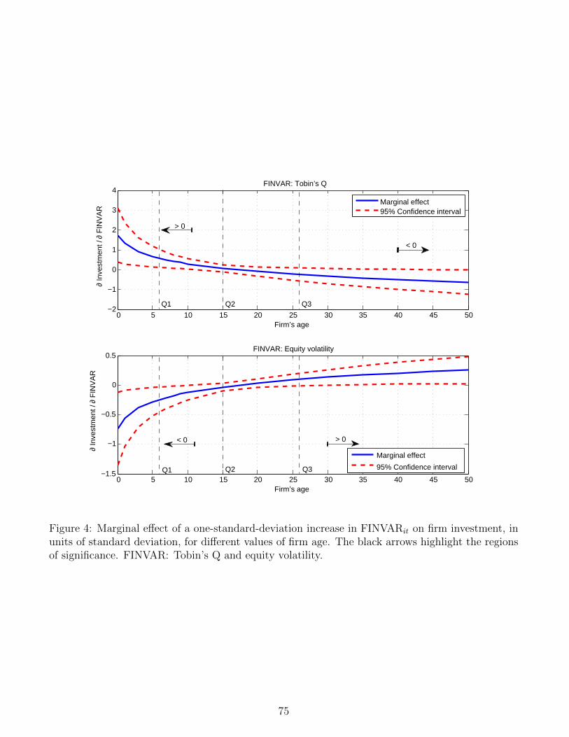
0 5 10 15 20 25 30 35 40 45 50−2

−1

0

1

2

3

4FINVAR: Tobin’s Q

∂ In

vest

men

t / ∂

FIN

VA

R

Firm’s age

Marginal effect95% Confidence interval

0 5 10 15 20 25 30 35 40 45 50−1.5

−1

−0.5

0

0.5FINVAR: Equity volatility

∂ In

vest

men

t / ∂

FIN

VA

R

Firm’s age

Marginal effect

95% Confidence interval

Q1 Q3Q2

Q1 Q2 Q3

< 0

> 0

< 0 > 0

Figure 4: Marginal effect of a one-standard-deviation increase in FINVARit on firm investment, inunits of standard deviation, for different values of firm age. The black arrows highlight the regionsof significance. FINVAR: Tobin’s Q and equity volatility.

75

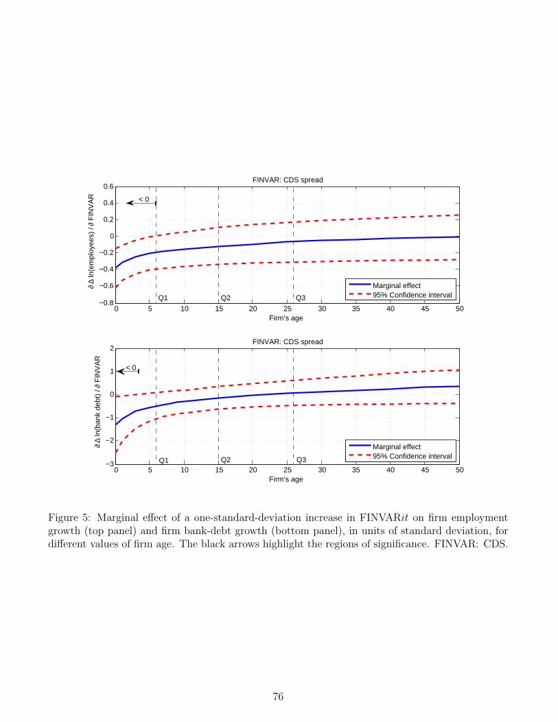
0 5 10 15 20 25 30 35 40 45 50−0.8

−0.6

−0.4

−0.2

0

0.2

0.4

0.6FINVAR: CDS spread

∂ ∆

ln(e

mpl

oyee

s) /

∂ F

INV

AR

Firm’s age

Marginal effect95% Confidence interval

0 5 10 15 20 25 30 35 40 45 50−3

−2

−1

0

1

2FINVAR: CDS spread

∂ ∆

ln(b

ank

debt

) / ∂

FIN

VA

R

Firm’s age

Marginal effect95% Confidence interval

Q1 Q3Q2

Q1 Q2 Q3

< 0

< 0

Figure 5: Marginal effect of a one-standard-deviation increase in FINVARit on firm employmentgrowth (top panel) and firm bank-debt growth (bottom panel), in units of standard deviation, fordifferent values of firm age. The black arrows highlight the regions of significance. FINVAR: CDS.

76