Financial Management

Liliya N. Zhilina, World Economy and Inrernational Relations Department, Vladivostok State University of Economic and Services (VSUES).

liliya.zhilina@vvsu.ru

8. Corporate Valuation and Value-Based Management.9. Capital budgeting. Risks Analysis.

8. Corporate Valuation and Value-Based Management

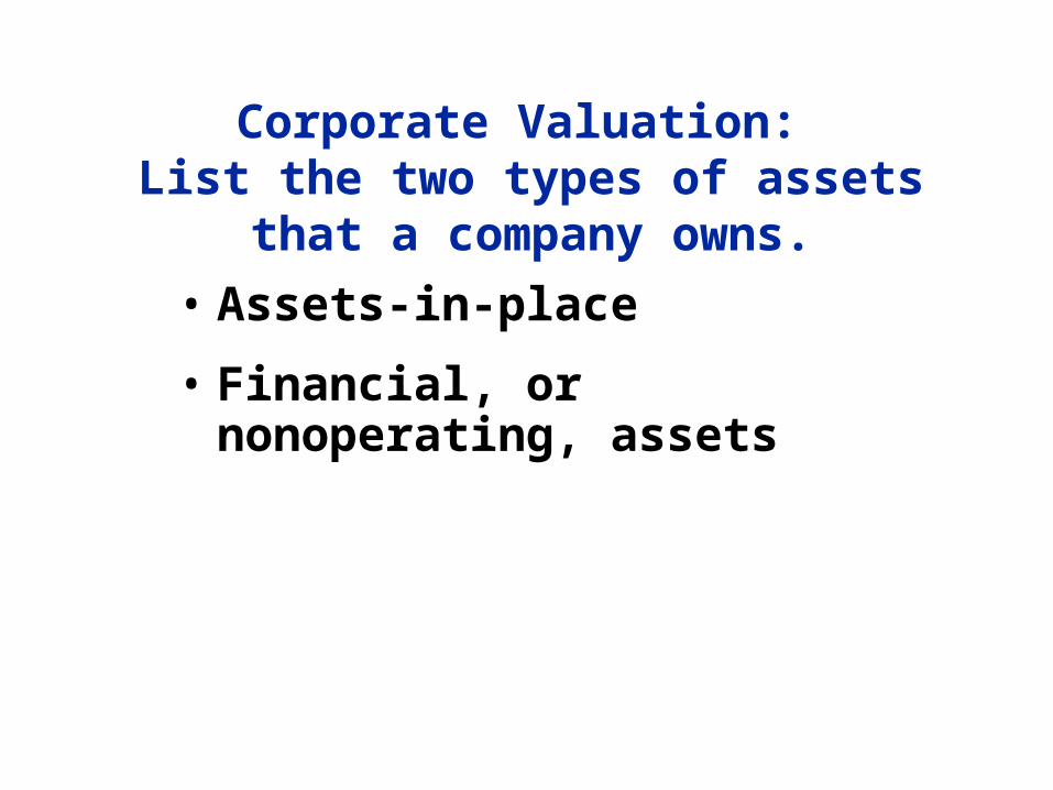
Corporate Valuation: List the two types of assets that a

company owns.

• Assets-in-place

• Financial, or nonoperating, assets

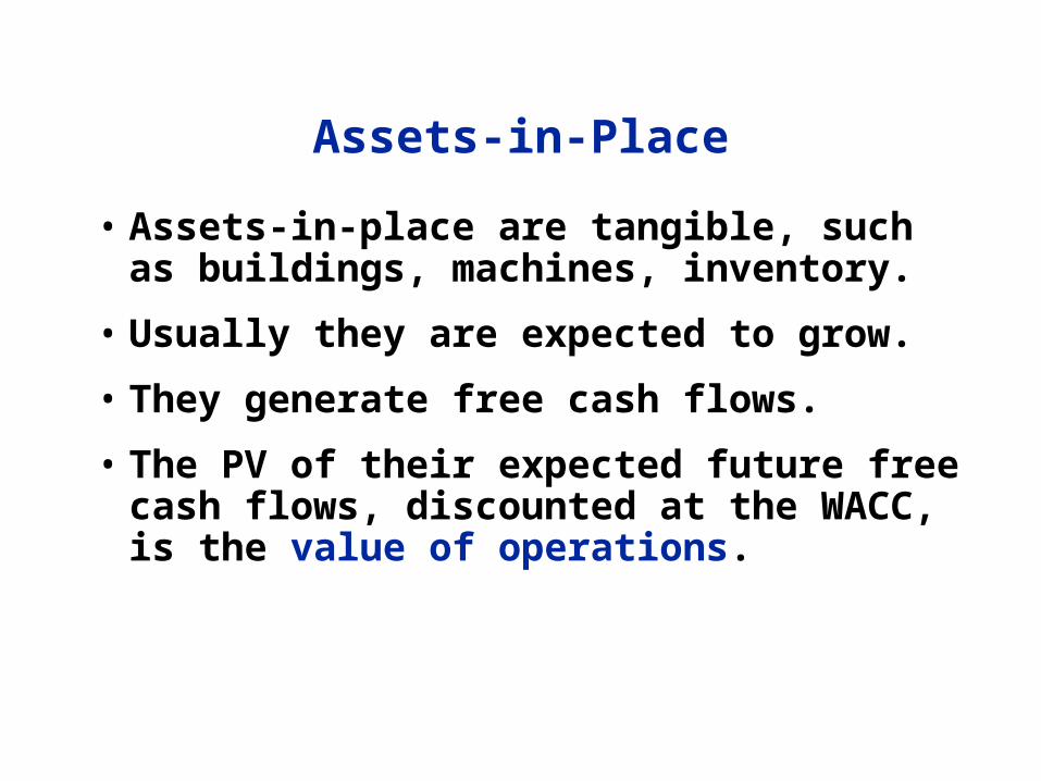
Assets-in-Place

• Assets-in-place are tangible, such as buildings, machines, inventory.

• Usually they are expected to grow.

• They generate free cash flows.

• The PV of their expected future free cash flows, discounted at the WACC, is the value of operations.

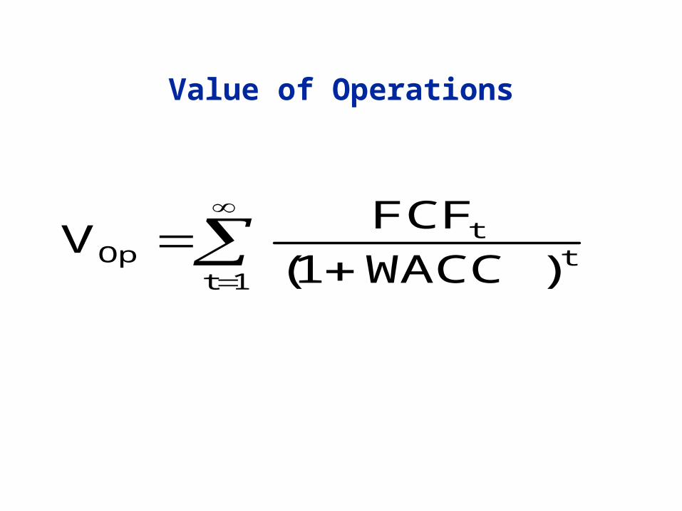
Value of Operations

1tt

tOp )WACC1(

FCFV

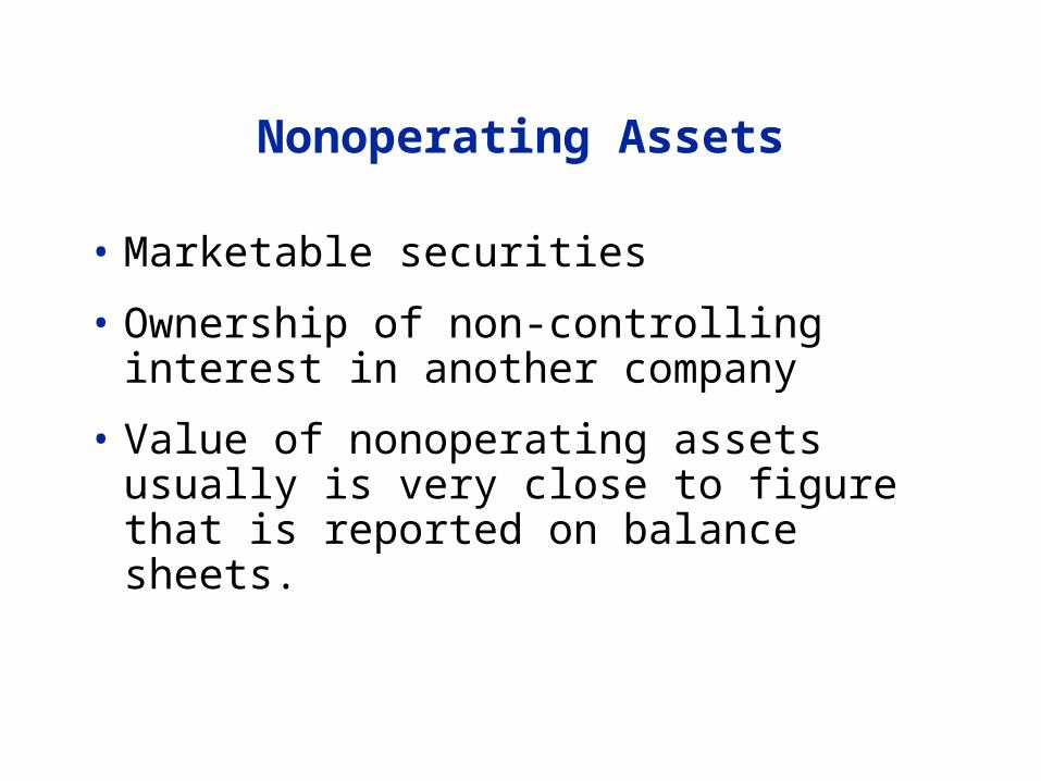
Nonoperating Assets

• Marketable securities

• Ownership of non-controlling interest in another company

• Value of nonoperating assets usually is very close to figure that is reported on balance sheets.

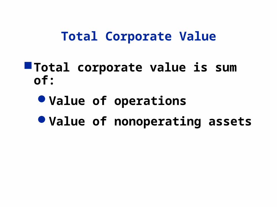
Total Corporate Value

Total corporate value is sum of:

Value of operations

Value of nonoperating assets

Claims on Corporate Value

• Debtholders have first claim.

• Preferred stockholders have the next claim.

• Any remaining value belongs to stockholders.

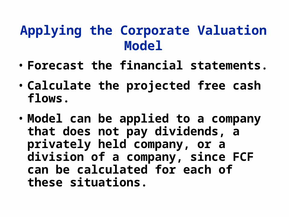
Applying the Corporate Valuation Model

• Forecast the financial statements.

• Calculate the projected free cash flows.

• Model can be applied to a company that does not pay dividends, a privately held company, or a division of a company, since FCF can be calculated for each of these situations.

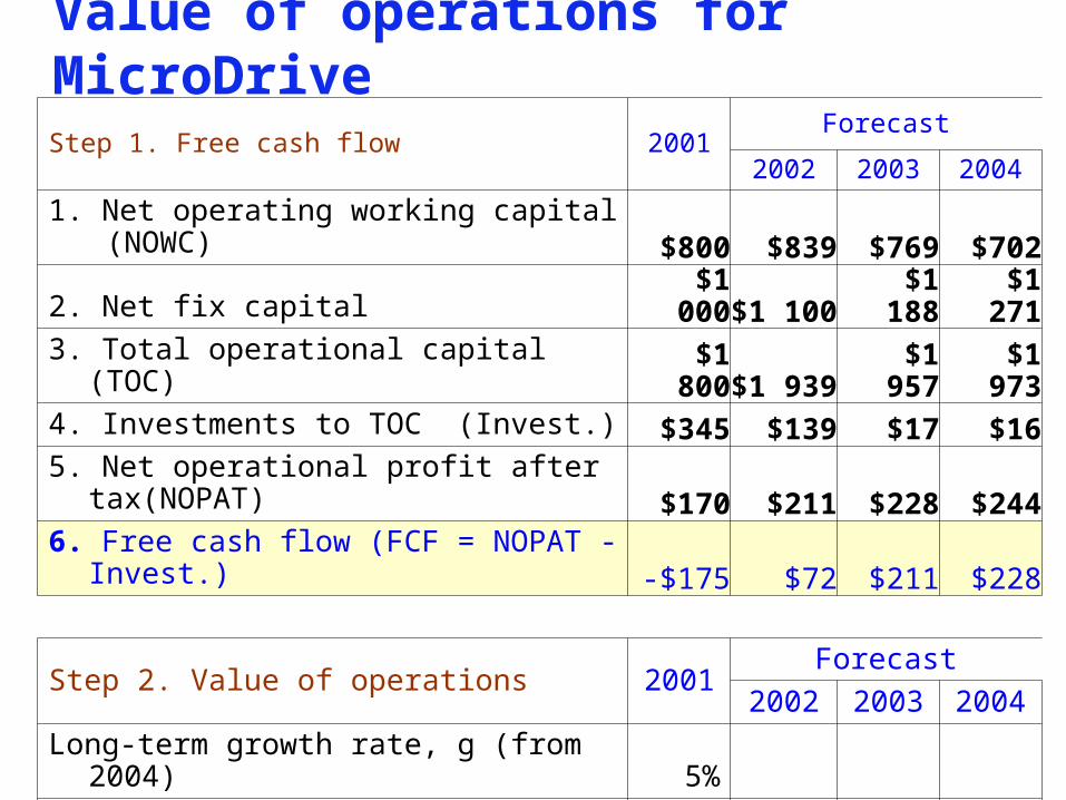
Value of operations for MicroDrive

Step 1. Free cash flow 2001Forecast

2002 2003 2004

1. Net operating working capital (NOWC) $800 $839 $769 $7022. Net fix capital $1 000 $1 100 $1 188 $1 2713. Total operational capital (TOC) $1 800 $1 939 $1 957 $1 9734. Investments to TOC (Invest.) $345 $139 $17 $165. Net operational profit after tax(NOPAT) $170 $211 $228 $2446. Free cash flow (FCF = NOPAT - Invest.) -$175 $72 $211 $228

Step 2. Value of operations 2001Forecast

2002 2003 2004

Long-term growth rate, g (from 2004) 5%      

WACC11,0

%      

FCF   $72 $211 $228

Vop at 3

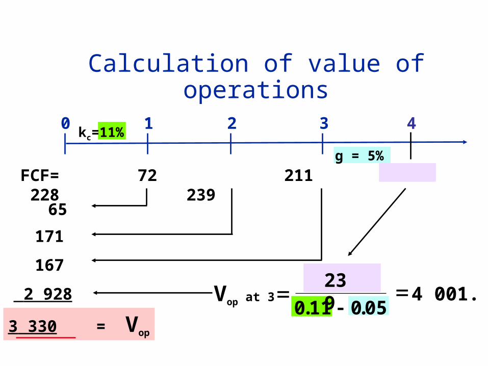
Calculation of value of operations

0

65

171

167

2 928

1 2 3 4kc=11%

3 330 = Vop

g = 5%

FCF= 72 211 228 239

239

. . 4 001.

11 0 05

0

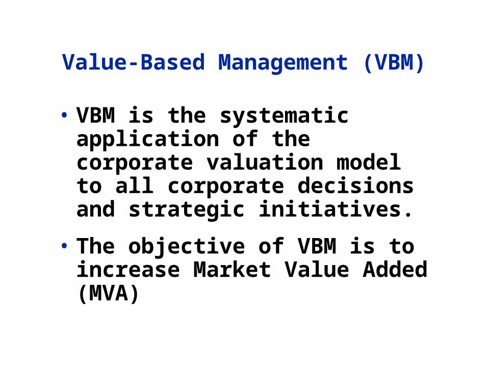
Value-Based Management (VBM)

• VBM is the systematic application of the corporate valuation model to all corporate decisions and strategic initiatives.

• The objective of VBM is to increase Market Value Added (MVA)

MVA and the Four Value Drivers

MVA is determined by four drivers:

Sales growth

Operating profitability (OP=NOPAT/Sales)

Capital requirements (CR=Operating capital / Sales)

Weighted average cost of capital

9. Capital budgeting. Cash Flow Estimation. Risk Analysis.

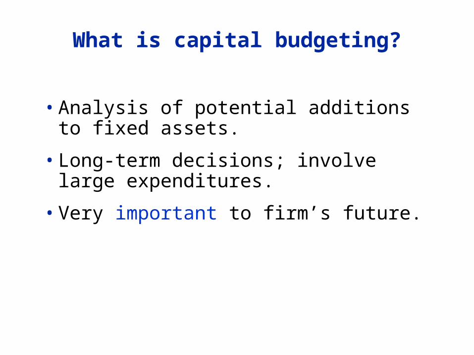
What is capital budgeting?

• Analysis of potential additions to fixed assets.

• Long-term decisions; involve large expenditures.

• Very important to firm’s future.

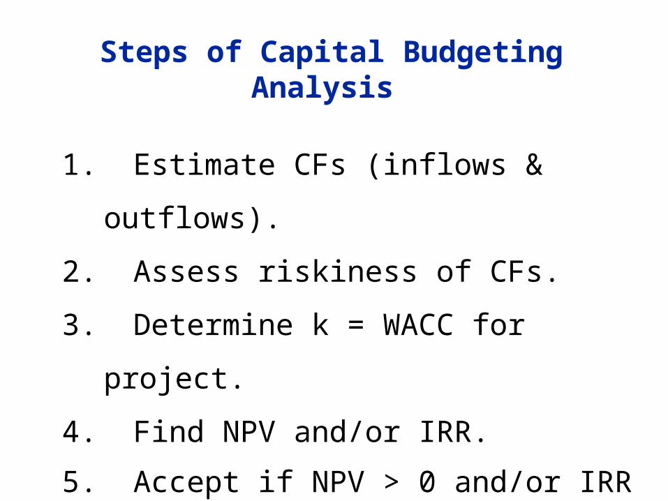
Steps of Capital Budgeting Analysis

1. Estimate CFs (inflows & outflows).

2. Assess riskiness of CFs.

3. Determine k = WACC for project.

4. Find NPV and/or IRR.

5. Accept if NPV > 0 and/or IRR > WACC.

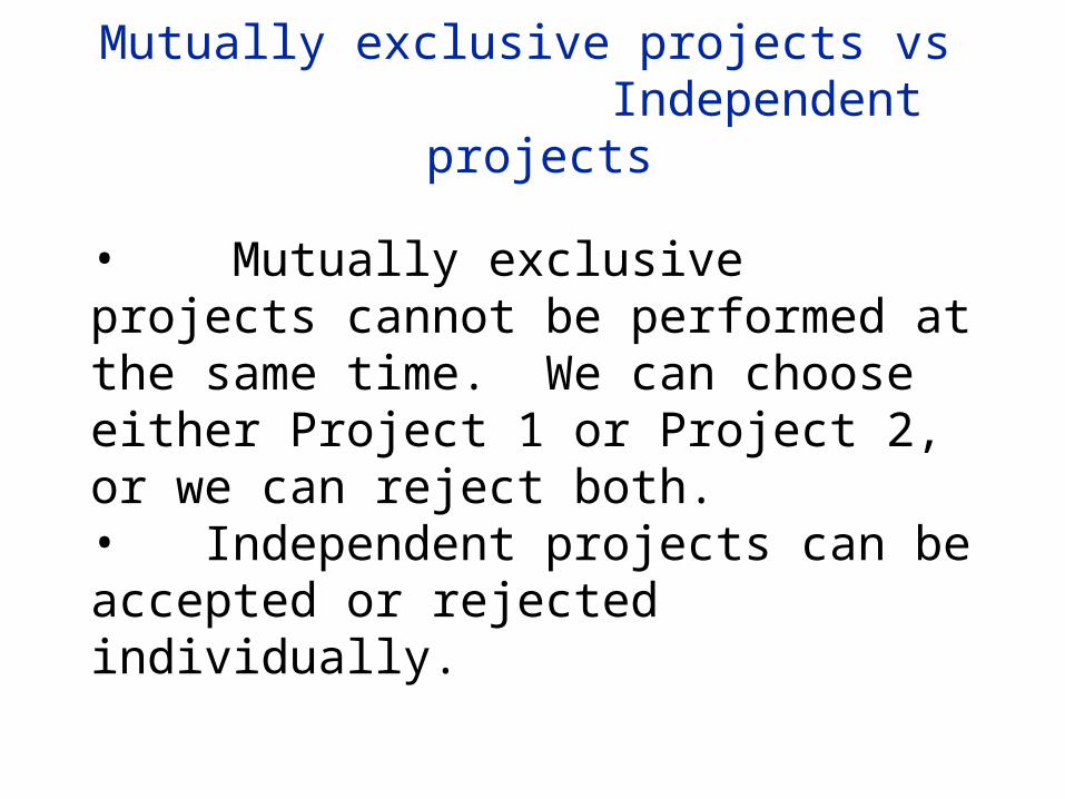
Mutually exclusive projects vs Independent projects

• Mutually exclusive projects cannot be performed at the same time. We can choose either Project 1 or Project 2, or we can reject both. • Independent projects can be accepted or rejected individually.

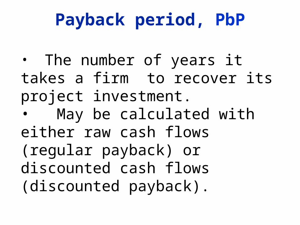
Payback period, PbP

• The number of years it takes a firm to recover its project investment. • May be calculated with either raw cash flows (regular payback) or discounted cash flows (discounted payback).

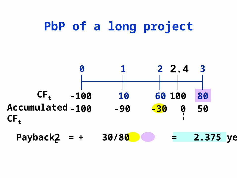
PbP of a long project

10 8060

0 1 2 3

-100

=

CFt

-100 -90 -30 50

PaybackL 2 + 30/80 = 2.375 years

0100

2.4

Accumulated CFt

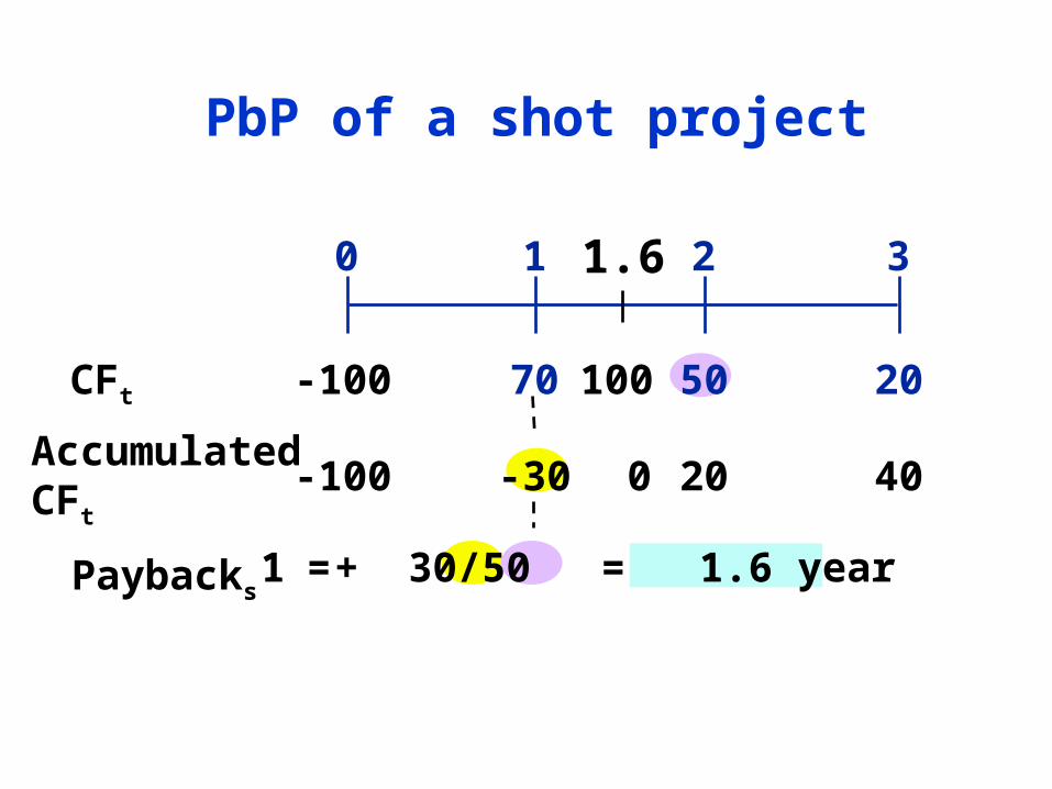
PbP of a shot project

70 2050

0 1 2 3

-100CFt

-100 -30 20 40

1 + 30/50 = 1.6 year

100

0

1.6

=

Accumulated CFt

Paybacks

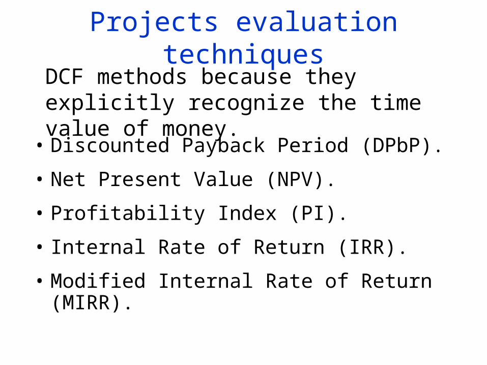
Projects evaluation techniques

• Discounted Payback Period (DPbP).

• Net Present Value (NPV).

• Profitability Index (PI).

• Internal Rate of Return (IRR).

• Modified Internal Rate of Return (MIRR).

DCF methods because they explicitly recognize the time value of money.

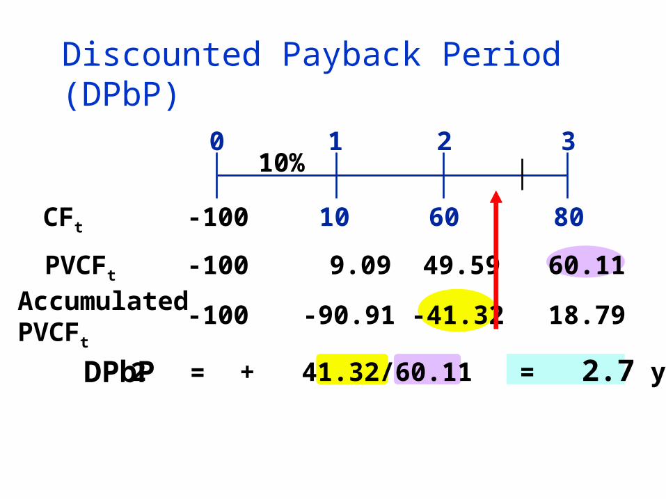
10 8060

0 1 2 3

CFt

Accumulated PVCFt

-100 -90.91 -41.32 18.79

DPbP 2 + 41.32/60.11 = 2.7 years

Discounted Payback Period (DPbP)

PVCFt -100

-100

10%

9.09 49.59 60.11

=

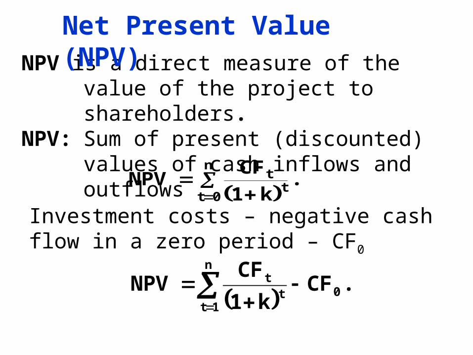
NPV

CF

kt

nt

t 0 1

.

NPV is a direct measure of the value of the project to shareholders.

NPV: Sum of present (discounted) values of cash inflows and outflows

Investment costs – negative cash flow in a zero period – CF0

.CF

k1

CFNPV 0t

tn

1t

Net Present Value (NPV)

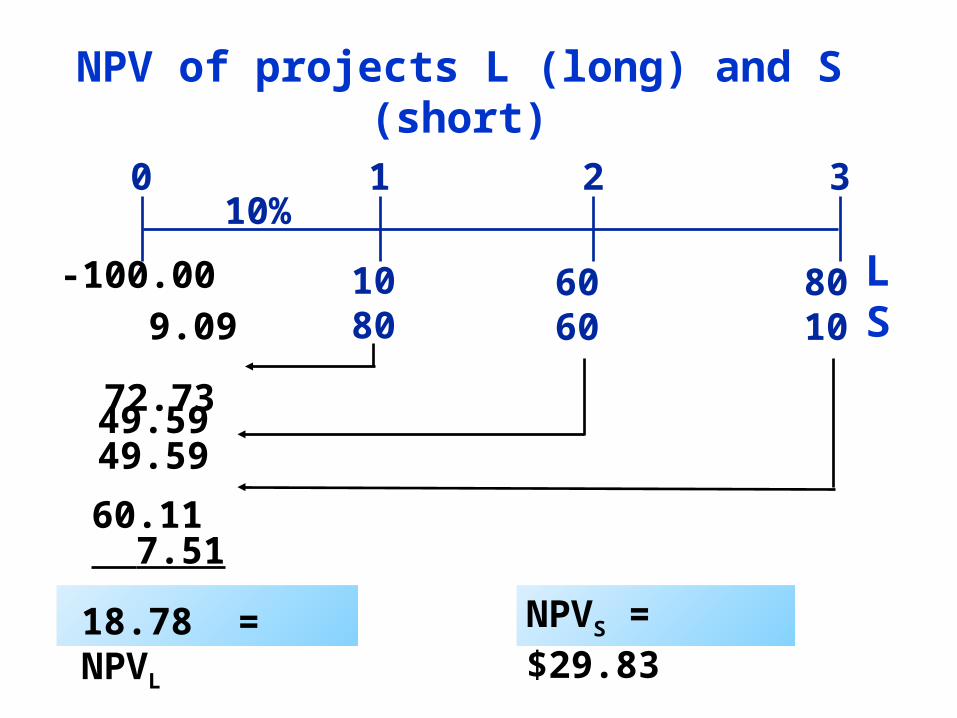
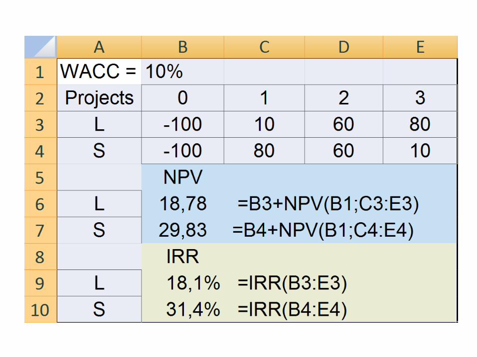
NPV of projects L (long) and S (short)

1080

8010

6060

0 1 2 310%

-100.00 9.09 72.73

49.5949.59

60.11 7.51

18.78 = NPVLNPVS = $29.83

LS

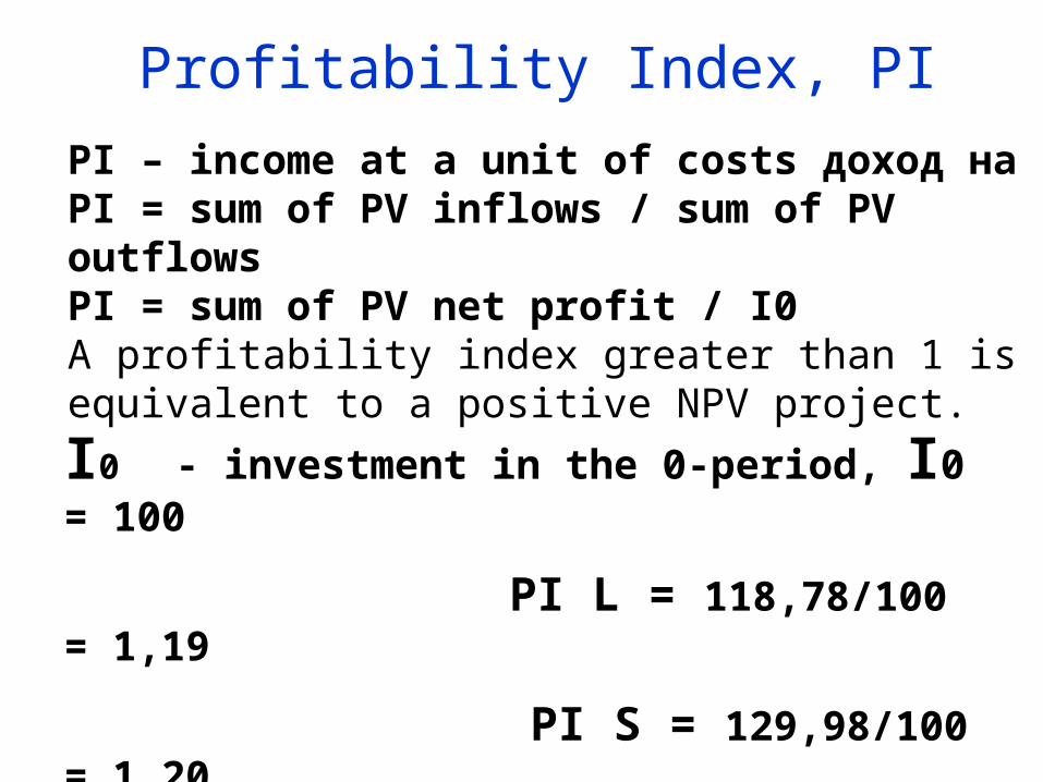
Profitability Index, PI

PI – income at a unit of costs доход наPI = sum of PV inflows / sum of PV outflowsPI = sum of PV net profit / I0A profitability index greater than 1 is equivalent to a positive NPV project.

I0 - investment in the 0-period, I0 = 100

PI L = 118,78/100 = 1,19

PI S = 129,98/100 = 1,20

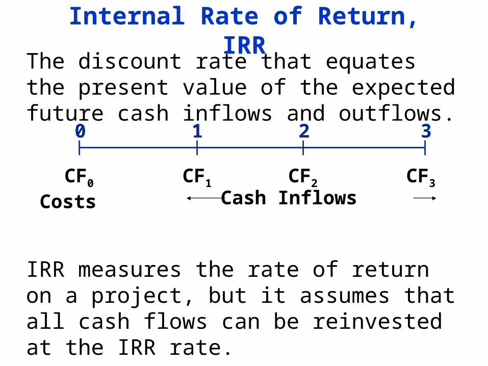
Internal Rate of Return, IRR

0 1 2 3

CF0 CF1 CF2 CF3

Costs Cash Inflows

The discount rate that equates the present value of the expected future cash inflows and outflows.

IRR measures the rate of return on a project, but it assumes that all cash flows can be reinvested at the IRR rate.

IRR проектов L и S

10 8060

0 1 2 3IRR = ?

-100.00

PV3

PV2

PV1

0 = NPV

IRRL = 18,1 % IRRS = 31,4 %

80 60 10L

S

Decision by IRR on S and L projects

• If S and L are independent projects they can be accepted (IRR > WACC).

• If S и L mutually exclusive projects we can choose Project S (IRRS > IRRL).

WACC = 10%

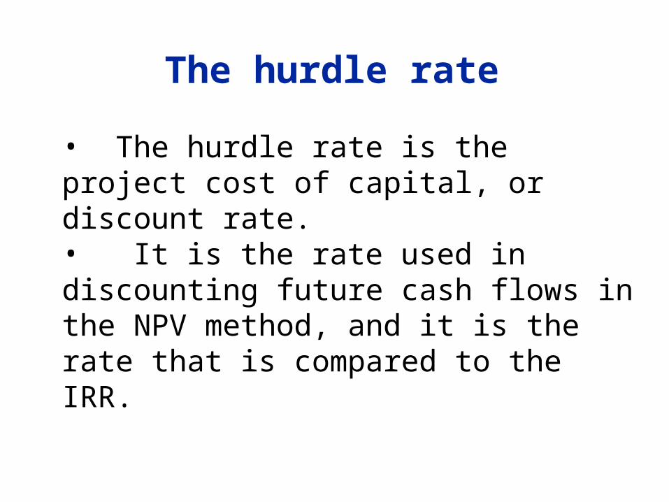
The hurdle rate

• The hurdle rate is the project cost of capital, or discount rate. • It is the rate used in discounting future cash flows in the NPV method, and it is the rate that is compared to the IRR.

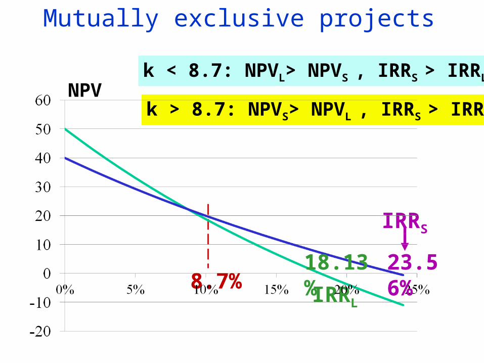
Mutually exclusive projects

8.7%

NPV

IRRS

IRRL

k < 8.7: NPVL> NPVS , IRRS > IRRL

k > 8.7: NPVS> NPVL , IRRS > IRRL

18.13% 23.56%

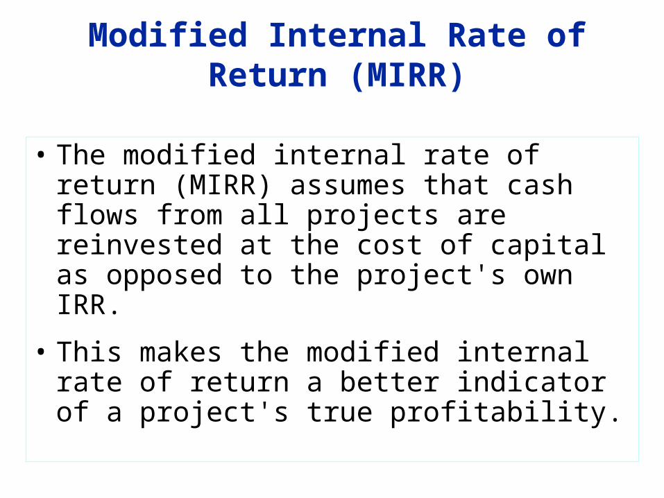
Modified Internal Rate of Return (MIRR)

• The modified internal rate of return (MIRR) assumes that cash flows from all projects are reinvested at the cost of capital as opposed to the project's own IRR.

• This makes the modified internal rate of return a better indicator of a project's true profitability.

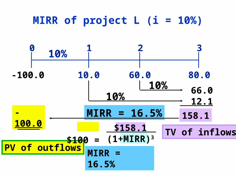
MIRR = 16.5%

10.0 80.060.0

0 1 2 310%

66.0 12.1

158.1

MIRR of project L (i = 10%)

-100.010%

10%

TV of inflows

-100.0

PV of outflowsMIRR = 16.5%

$100 = $158.1(1+MIRR)3

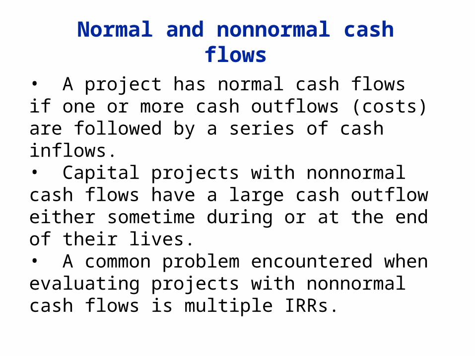
Normal and nonnormal cash flows

• A project has normal cash flows if one or more cash outflows (costs) are followed by a series of cash inflows.• Capital projects with nonnormal cash flows have a large cash outflow either sometime during or at the end of their lives. • A common problem encountered when evaluating projects with nonnormal cash flows is multiple IRRs.

 

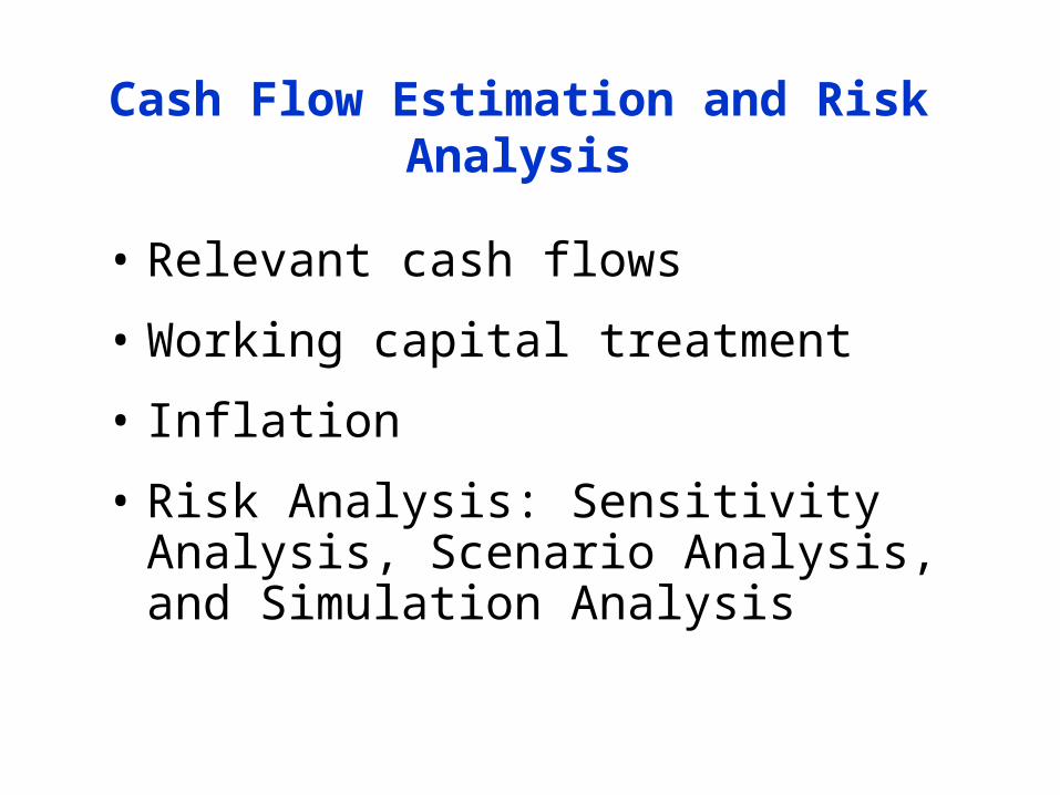
• Relevant cash flows

• Working capital treatment

• Inflation

• Risk Analysis: Sensitivity Analysis, Scenario Analysis, and Simulation Analysis

Cash Flow Estimation and Risk Analysis

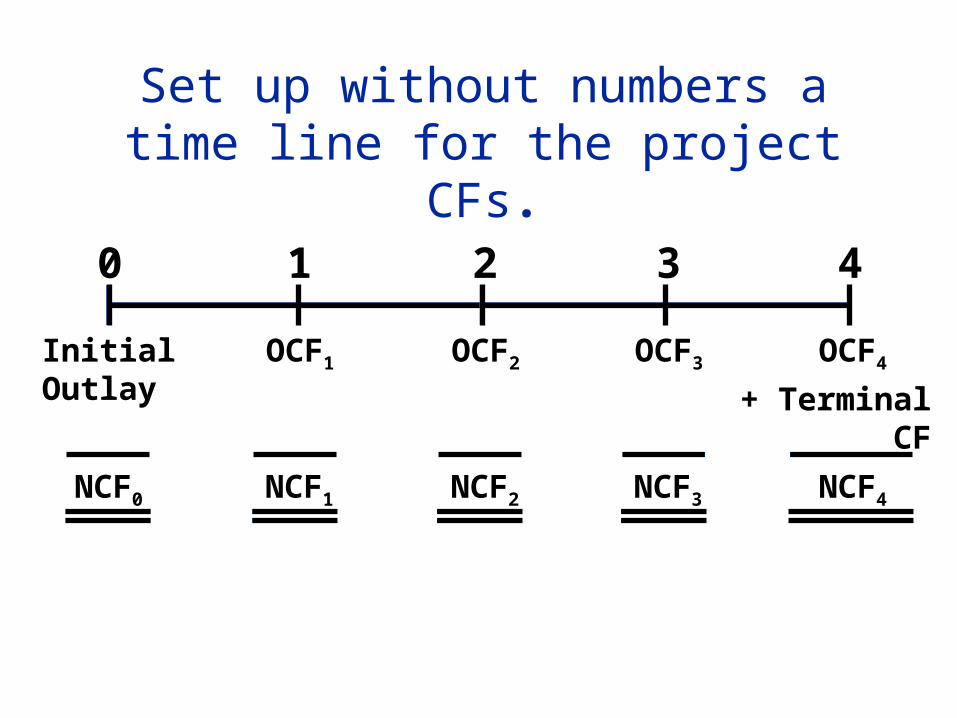
Set up without numbers a time line for the project CFs.

0 1 2 3 4

InitialOutlay

OCF1 OCF2 OCF3 OCF4

+ Terminal CF

NCF0 NCF1 NCF2 NCF3 NCF4

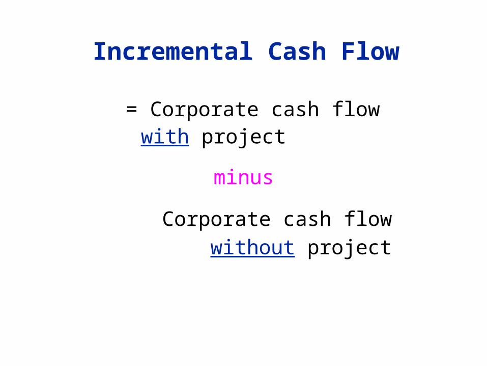
= Corporate cash flow with project

minus

Corporate cash flow

without project

Incremental Cash Flow

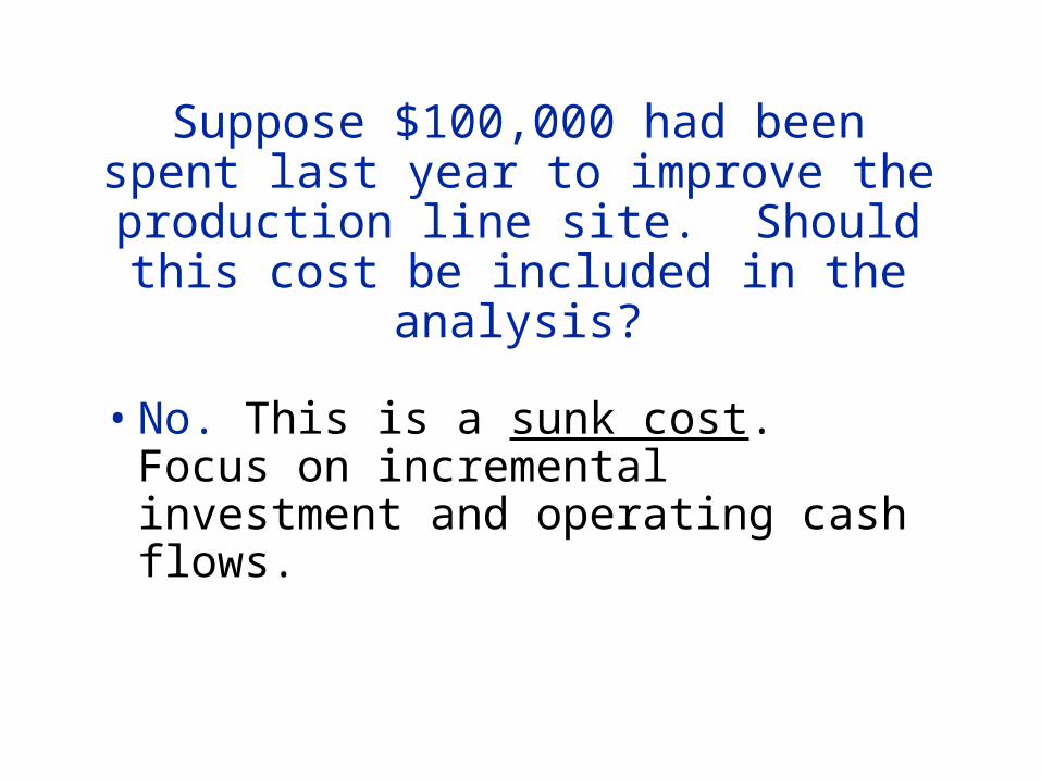
• No. This is a sunk cost. Focus on incremental investment and operating cash flows.

Suppose $100,000 had been spent last year to improve the production line site.

Should this cost be included in the analysis?

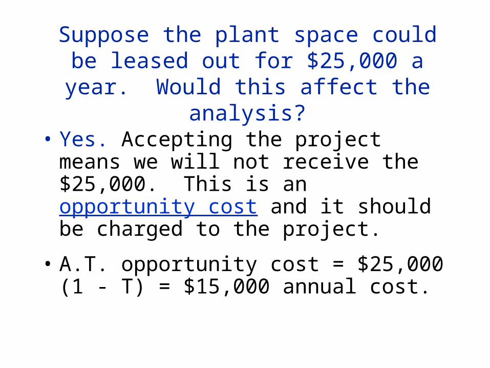
• Yes. Accepting the project means we will not receive the $25,000. This is an opportunity cost and it should be charged to the project.

• A.T. opportunity cost = $25,000 (1 - T) = $15,000 annual cost.

Suppose the plant space could be leased out for $25,000 a year. Would this affect

the analysis?

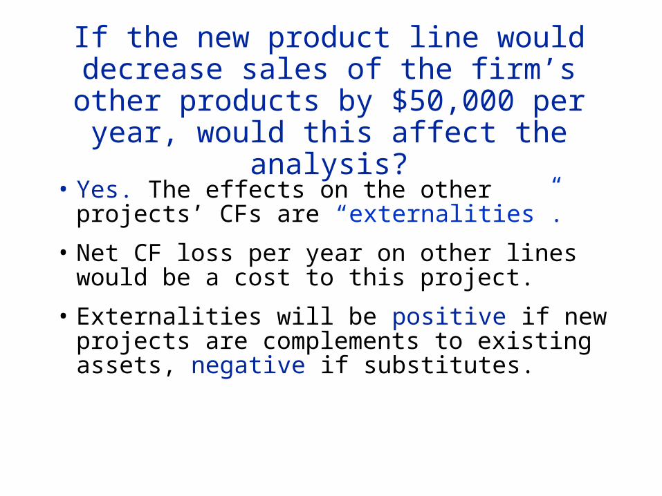
• Yes. The effects on the other projects’ CFs are “externalities”.

• Net CF loss per year on other lines would be a cost to this project.

• Externalities will be positive if new projects are complements to existing assets, negative if substitutes.

If the new product line would decrease sales of the firm’s other products by

$50,000 per year, would this affect the analysis?

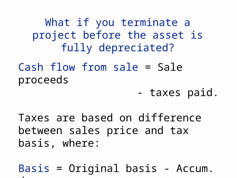
What if you terminate a project before the asset is fully depreciated?

Cash flow from sale = Sale proceeds- taxes paid.

Taxes are based on difference between sales price and tax basis, where:

Basis = Original basis - Accum. deprec.

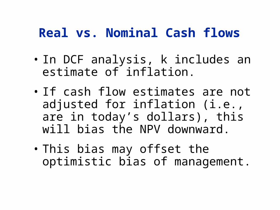
• In DCF analysis, k includes an estimate of inflation.

• If cash flow estimates are not adjusted for inflation (i.e., are in today’s dollars), this will bias the NPV downward.

• This bias may offset the optimistic bias of management.

Real vs. Nominal Cash flows

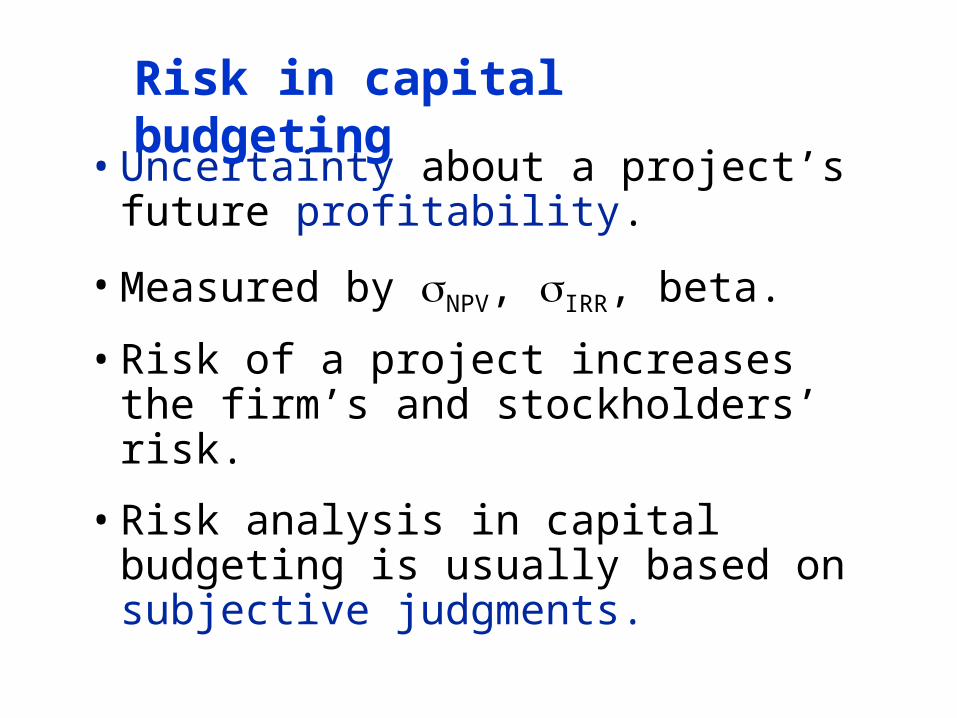
• Uncertainty about a project’s future profitability.

• Measured by NPV, IRR, beta.

• Risk of a project increases the firm’s and stockholders’ risk.

• Risk analysis in capital budgeting is usually based on subjective judgments.

Risk in capital budgeting

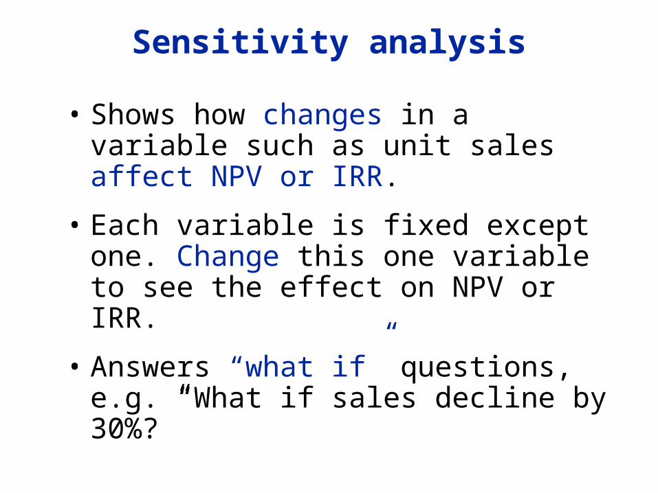
• Shows how changes in a variable such as unit sales affect NPV or IRR.

• Each variable is fixed except one. Change this one variable to see the effect on NPV or IRR.

• Answers “what if” questions, e.g. “What if sales decline by 30%?”

Sensitivity analysis

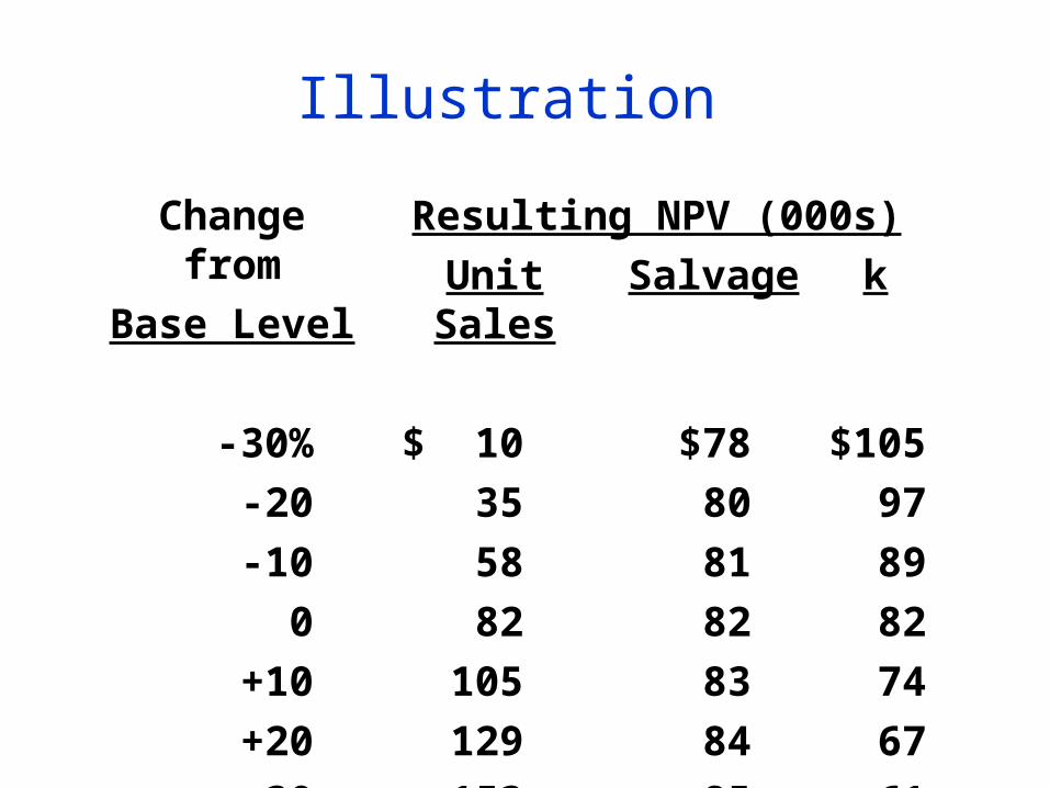
Change from

Base Level

Resulting NPV (000s)

Unit Sales Salvage k

-30% $ 10 $78 $105

-20 35 80 97

-10 58 81 89

0 82 82 82

+10 105 83 74

+20 129 84 67

+30 153 85 61

Illustration

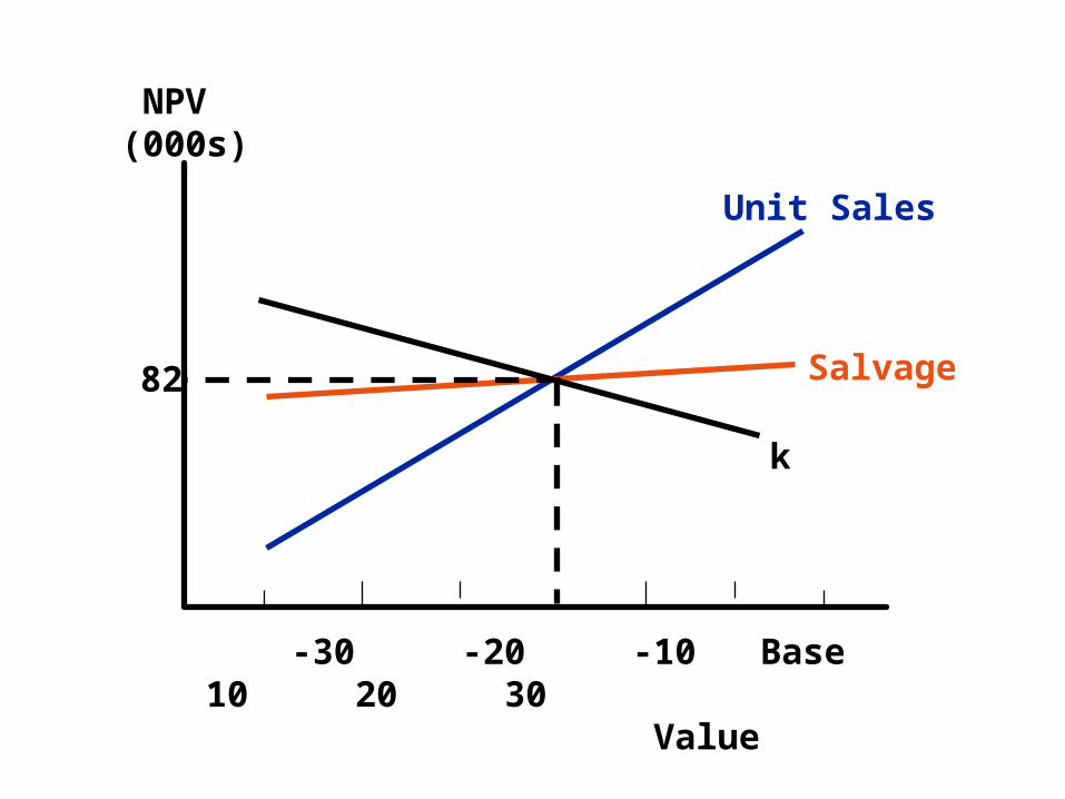
-30 -20 -10 Base 10 20 30 Value

82

NPV(000s)

Unit Sales

Salvage

k

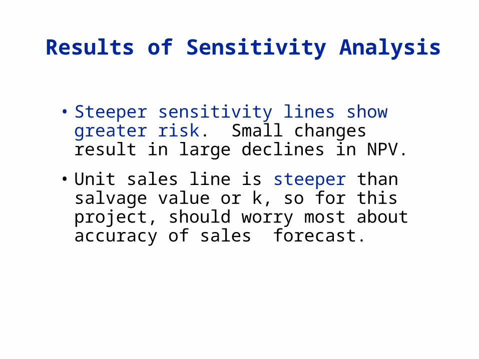
• Steeper sensitivity lines show greater risk. Small changes result in large declines in NPV.

• Unit sales line is steeper than salvage value or k, so for this project, should worry most about accuracy of sales forecast.

Results of Sensitivity Analysis

• Does not reflect diversification.

• Says nothing about the likelihood of change in a variable, i.e. a steep sales line is not a problem if sales won’t fall.

• Ignores relationships among variables.

Weaknesses ofsensitivity analysis

• Gives some idea of stand-alone risk.

• Identifies dangerous variables.

• Gives some breakeven information.

Why is sensitivity analysis useful?

• Examines several possible situations, usually worst case, most likely case, and best case.

• Provides a range of possible outcomes.

Scenario analysis

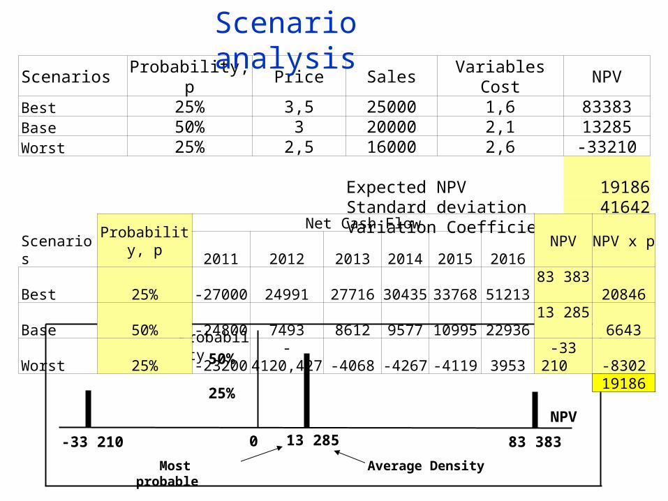
-33 210 0 83 38313 285

Average Density Most probable

NPV

Probability

50%

25%

Scenarios Probability, p Price Sales Variables Cost NPVBest 25% 3,5 25000 1,6 83383Base 50% 3 20000 2,1 13285Worst 25% 2,5 16000 2,6 -33210

Expected NPV 19186Standard deviation 41642Variation Coefficient 2,17

ScenariosProbability, p

Net Cash FlowNPV NPV x p

2011 2012 2013 2014 2015 2016Best 25% -27000 24991 27716 30435 33768 51213 83 383 20846Base 50% -24800 7493 8612 9577 10995 22936 13 285 6643Worst 25% -23200 -4120,427 -4068 -4267 -4119 3953 -33 210 -8302

19186

Scenario analysis

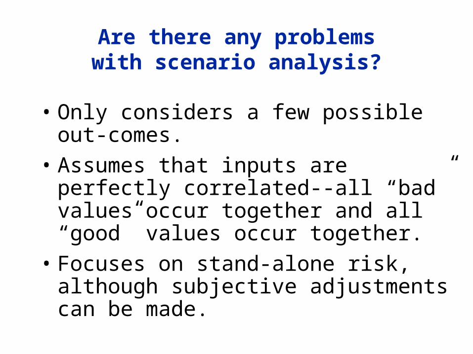
• Only considers a few possible out-comes.

• Assumes that inputs are perfectly correlated--all “bad” values occur together and all “good” values occur together.

• Focuses on stand-alone risk, although subjective adjustments can be made.

Are there any problems with scenario analysis?

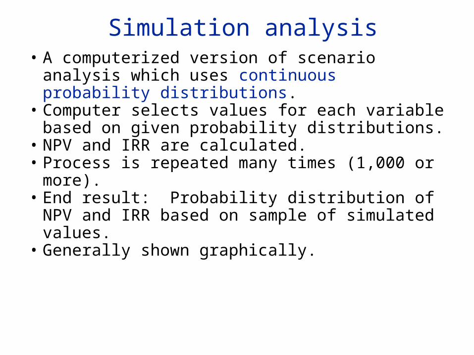
• A computerized version of scenario analysis which uses continuous probability distributions.

• Computer selects values for each variable based on given probability distributions.

• NPV and IRR are calculated.• Process is repeated many times (1,000 or

more).• End result: Probability distribution of NPV and

IRR based on sample of simulated values.• Generally shown graphically.

Simulation analysis

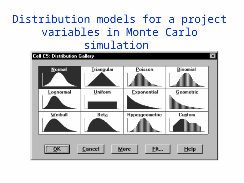
Distribution models for a project variables in Monte Carlo simulation

Probability Density (NPV)

Also gives NPV, CVNPV, probability of NPV > 0.

0 E(NPV) NPV

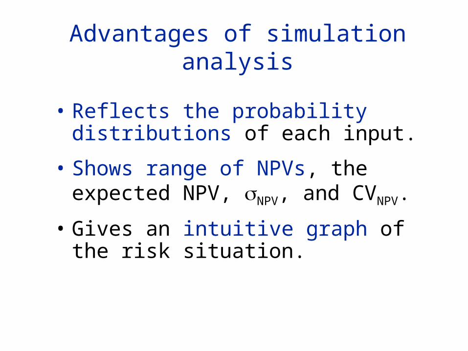
• Reflects the probability distributions of each input.

• Shows range of NPVs, the expected NPV, NPV, and CVNPV.

• Gives an intuitive graph of the risk situation.

Advantages of simulation analysis

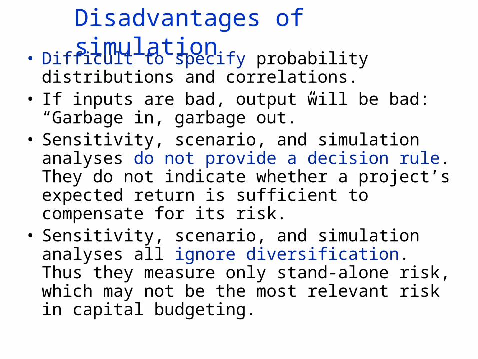
• Difficult to specify probability distributions and correlations.

• If inputs are bad, output will be bad:“Garbage in, garbage out.”

• Sensitivity, scenario, and simulation analyses do not provide a decision rule. They do not indicate whether a project’s expected return is sufficient to compensate for its risk.

• Sensitivity, scenario, and simulation analyses all ignore diversification. Thus they measure only stand-alone risk, which may not be the most relevant risk in capital budgeting.

Disadvantages of simulation