FINANCIAL LIBERALISATION - Journal€¦ · Web view), Dutt (1990) and Burkett and Dutt (1991) Using Tobin’s portfolio framework for household, thus household choice of investments

INTEREST RATE LIBERALISATION AND ECONOMIC GROWTH IN NIGERIA: EVIDENCE BASED ON ARDL-BOUNDS TESTING

APPROACH1

Erasmus L. Owusu2

University of South Africa (UNISA)12 Rosedale Close, Redditch, B97 6JQ, UK.

Email: [email protected]

And

Prof. Nicholas M. OdhiamboDepartment of EconomicsUniversity of South Africa

P.O Box 392, UNISA0003, PretoriaSouth Africa

Email: [email protected]/ [email protected]

(A manuscript submitted for publication)

August 2011

1 This paper is based on my doctoral research at the University of South Africa (UNISA). The usual disclaimer applies.2 Corresponding Author.

mailto:[email protected]

mailto:[email protected]/

mailto:[email protected]

INTEREST RATE LIBERALISATION AND ECONOMIC GROWTH IN NIGERIA: EVIDENCE BASED ON ARDL-BOUNDS TESTING

APPROACH

Abstract

This paper examines the relationship between interest rate liberalisation policies and sustainable economic

growth in Nigeria. Employing autoregressive distributed lag (ARDL) - bounds testing approach and using

GDP per capita as growth indicator, the paper establishes a long run relationship between economic growth

and interest rate liberalisation which is represented by an index calculated using principal component

analysis (PCA). The paper finds that in the long run, interest rate liberalisation policies have positive effect

on economic growth in Nigeria. This supports the numerous past studies which have reported positive

results regarding the effects of interest rate liberalisation on economic growth. The paper concludes that

interest rate liberalisation polices together with increase in the productivity of labour, increase in capital

stock and increase in foreign direct investments determine economic growth in Nigeria.

Keywords:

Economic Growth, Interest Rate Liberalisation, ARDL-Bounds Testing Approach, Cointegration and

Nigeria.

1 Introduction

McKinnon (1973) and Shaw (1973) were the first to suggest theoretical arguments against the policies of

financial repression. They pointed out the important role of the financial sector in increasing the volume of

savings as a result of creating appropriate incentives. In order to reach higher savings and hence investment

rates, McKinnon (1973) and Shaw (1973) argue that governments should abolish interest rate ceilings and

allow real interest rates to be determined by the market. This they argue, will lead to increase in savings

and hence investment and ultimately leading to economic growth as well as bringing inflation down

(Gibson and Tsakalotos, 1994). Based on this hypothesis, many governments in the developing countries

liberalised their interest rate with some achieving significant accelerations in economic growth rates but in

some cases the policy was associated with excessively high and volatile real interest rates as well as

stagflation (Grabel, 1995). Van Wijnbergen (1983) contrasts his hypothesis to those of McKinnon (1973)

and Kapur (1976). He expresses the view that the outcome of McKinnon-Kapur depends crucially on one

implicit assumption on asset market structure, an assumption that is never stated explicitly: that the

portfolio shift into bank deposit is coming out of “unproductive” assets like gold, cash or inventories. Van

Wijnbergen (1983) further argues that it is not at all obvious that bank deposits are closer substitute to cash

or gold rather to loan extended on the informal sector. Stiglitz (1989) also criticises the policy of financial

liberalisation3 on the theoretical ground of market failures in financial markets.

The purpose of this paper is to empirically investigate and provide insight into the impact of interest rate

liberalisations on sustainable economic growth in Nigeria (a member of the Economic Community of West

African States - ECOWAS4). In this investigation, the paper constructs an interest rate liberalisation index

factor5 which encompasses all the relevant policies of interest rate liberalisation taken in Nigeria using

principal component analysis (PCA). The paper employs the more efficient univariate DF-GLS test for

autoregressive and the Phillips and Peron (PP) unit root tests rather than the conversional augmented

Dickey-Fuller (ADF) to test for the stationarity of the variables used in this study. After that the paper

applies the empirical analytical method of autoregressive distributed lag (ARDL) – Bounds testing

approach in an attempt to establish a long term relationship between interest rate liberalisation and

sustainable economic growth using time series data. Lastly, a dynamic unrestricted error correction model

(UECM) will be derived from the ARDL – Bounds testing models. The sources of the data include

various issues of World Bank’s World Development Indicators, World Bank’s African

Development Indicators, IMF’s International Financial Statistics, Central Bank of

Nigeria, Nigerian Office of Federal Statistics and other relevant sources. Furthermore,

3Note that financial liberalisation and interest rate liberalisation is used interchangeably.4The Economic Community of West African States is made up of 15 countries in the in the West African sub-region, namely: Benin, Burkina Faso, Cape Verde, Cote d’Ivoire, Gambia, Ghana, Guinea-Bissau, Guinea, Liberia, Mali, Niger, Nigeria, Senegal, Sierra

Leone and Togo.5This factor will be used instead of dummies to represent the effect of interest rate liberalisation policies in Nigeria. A similar approach was employed by Caprio et al (2001) and Laeven (2003).

this paper contributes to the literature on interest rate liberalisation by establishing whether interest rate

liberalisation has any positive influence on economic growth in Nigeria. This paper uses data from 1969

and 2008, thus covering both the periods of financial repression and interest rate liberalisation. However,

the main period of this paper is the post liberalisation periods. The motivation for using the interest rate

liberalisation index factors is to ensure that all the various interest rate liberalisation policies implemented

towards the attainment of full financial liberalisation status are taken into accounts for Nigeria and also to

help solve the problem of quantification of the effect of interest rate liberalisation which is usually one of

the problems associated with empirical studies in this area (Caprio et al, 2001; Laeven, 2003).

Moreover, most of the earlier studies completed on interest rate liberalisation and economic growth are

based on evidence from Latin American and the East Asian countries with little attention devoted to

African countries, especially, primary commodity exporter countries in the region like Nigeria. The

potential weakness of this paper is that the results should be applied to any other country with caution This

paper is among the first to examine in detail the dynamic impact of interest rate liberalisation on economic

growth in a primary commodity exporter countries, Nigeria, using constructed interest rate liberalisation

index and the ARDL – Bounds testing approach by looking at the effects of interest rate liberalisation on

economic growth. This paper is divided into six sections including the introduction. In section two, the

paper reviews the interest rate liberalisation policies in Nigeria. This is followed in section three with the

literature review, both theoretical and empirical. In section four, the paper looks at the methodology and the

empirical analysis. The conclusion comes in section five followed by references.

2 Overview of interest rate liberalisation policy in Nigeria

The Structural Adjustment Programme (SAP) was adopted in 1986 against the background of international

oil market crashes and the resultant deteriorating economic conditions in the country. It was designed to

achieve fiscal balance and balance of payments viability by altering and restructuring the production and

consumption patterns of the economy, eliminating price distortions, reducing the heavy dependence on

crude oil exports and consumer goods imports, enhancing the non-oil export base and achieving sustainable

growth. Other aims were to rationalise the role of the public sector and accelerate the growth potentials of

the private sector. The main strategies of the programme were the deregulation of external trade and

payments arrangements, the adoption of a market determined exchange rate for the Naira, substantial

reduction in complex price and administrative controls and more reliance on market forces as a major

determinant of economic activity (Adebiyi, 2005). With the switch to indirect instruments came the change

of the goal of monetary policy to the reduction of inflation. This change was prompted by the belief that

monetary policy has only temporal effects on real variables and long run effects on prices (Ibid). Empirical

evidence over the years has shown that low inflation is a prerequisite for economic growth. Given the high

levels of inflation in the country at the time especially after the implementation of the reforms policy, there

was the need to bring inflation under control before a sustained path to growth could be attained. Using the

implementation of policy in line with the IMF financial programming framework, control of growth in

money supply became a very important factor in the fight against rampant inflation (Ibid). Targets were set

each year for growth in broad money and inflation rate. The implementation of the policy has involved

monitoring the deviation of growth in money from target. Controlling the growth of money supply proved

to be a difficult task especially in the years just after financial deregulation (Adebiyi, 2005; Ojo, 2001).

3 Theoretical and Empirical literature review

3.1 Theoretical issues

The main proponents of the McKinnon-Shaw hypothesis are Kapur (1976), Matheison (1980), Galbis

(1977) and Jao (1985) among others. Kapur (1976), for example, examines the impact of interest rate

liberalisation in an economy characterised by under-utilised fixed capital and surplus labour. He argues

that the real supply of credits affect capital accumulation through its role as the sole source of finance for

working capital requirements. Real credit supply is determined by the demand for broad money which

itself is a function of inflation and the deposit rate of interest. A rise in the deposit rate works more

indirectly on the supply of credits and hence the supply of banks deposits increases. This allows banks to

give more credits (Ibid). Mathieson (1980) model is similar to that of Kapur (1976) with the only difference

being that bank credits finances are not only net additions to working capital but also to fixed assets. In

both Kapur (1976) and Mathieson (1980), increased growth is the result of an increase in the quantity of

investment whiles McKinnon and Shaw’s growth is as a result of increase in the quality and quantity of

investments (Gibson and Tsakalotos, 1994).

The principal critics of the McKinnon-Shaw hypothesis are Van Wijnbergen (1983) and Taylor (1983)6.

Using Tobin’s portfolio framework for household, thus household choice of investments includes time

deposit, loans to business through the informal sector and gold or currency, they argue that in response to

increase in interest rate on deposits, household will substitute these for gold or cash and loans in the

informal sector. Van Wijnbergen (1983) contrasts his model to those of McKinnon (1973) and Kapur

(1976). He expresses the view that the outcomes of McKinnon-Kapur models depend crucially on one

implicit assumption on asset market structure, an assumption that is never stated explicitly: that the

portfolio shift into bank deposit is coming out of “unproductive” assets like gold or cash, inventories. He

further argues that it is not at all obvious that bank deposit are closer substitute to cash, gold, livestock and

other commodities but rather to loan extended on the informal sector (Gibson and Tsakalotos, 1994).

3.2 Some Empirical Evidence

Empirical evidence of the McKinnon-Shaw hypothesis has been shown to have rather mixed results. This

may be an indication that interest rate liberalisation policy alone is a necessary but an insufficient condition

for sustainable economic growth in developing countries. Most of the evidence of interest rate liberalisation

hypothesis seem to suggest a significantly improvement in the quality of investment but not in the quantity

of investment and the volume of savings. One thing which seems to be clear from the available evidence is

that in addition to macroeconomic stabilisation, sound and proven regulation of the financial sector seems

to play an important role for the successful implementation of the interest rate liberalisation policy. Roubini

and Sala-i-Martin (1992) using a cross-section data from 98 countries for the period of 1960-1985, show

that various measures of financial repression affect growth negatively. They also find empirical support for

the hypothesis that real interest rates below -5% as well as moderately negative real interest rates are

significantly associated with low economics growth rates. They interpret this as an indication that only

severe financial repression inhibits growth. Other writers have also used panel data (for example, Seck and

6See also Grabel (1995, 1994), Studart (1996), Dutt (1990) and Burkett and Dutt (1991)

El Nil, 1993; Charlier and Oguie, 2002; Allen and Ndikumana, 2000.) to investigate the relationship

between interest rate liberalisation and economic growth in Africa (Fowowe, 2002). Seck and El Nil (1993)

and Charlier and Oguie (2002), for instance, find a significant positive relationship between economic

growth and the real interest rate liberalisation (ibid).

There are various studies which results are inconclusive or are against the financial liberalisation

hypothesis. For example, Goldsmith (1969) using sample data from 35 countries over a period from 1860-

1963, reports a rough or inconclusive correlation between interest rate liberalisation and economic growth.

In King and Levine (1993), the authors specifically stated that about one third of the difference between

very fast and very slow growing economies can be removed by increasing the depth of the financial

intermediation sector. Bhatia and Khatkhate (1975) using correlation graphs to examine the relationship

between economic growth and interest rate liberalisation in eleven African countries find no definite

relationship between economic growth and financial liberalisation for the studied countries either

individually, or for the whole group. Also, Ogun (1986) using cross sectional analysis on data for 20

countries in Africa from 1969 – 1983 estimates the correlation between interest rate liberalisation and

economic growth and finds no support to the economic growth enhancing capabilities of financial

liberalisation.

4 Methodology and Empirical Analysis

4.1 Methodology

According to McKinnon (1973) and Shaw (1973), interest rate liberalisation spurs

economic growth through the efficiency of the financial sector. They are of the view

that increase in savings, increase in financial deepening and increase in investment

are some of the long term impact of interest rate liberalisation policy. In line with

this, the paper adopts the models used by Shrestha and Chowdhury (2007) to test

the effect of interest rate liberalisation on savings, investments and ultimately,

economic growth. However, in place of using time deposits held at the banks as a

proxy for savings, total bank credits as a proxy of investments and real GDP, the

paper uses real total financial savings7 (TFS), credit to the private sector (CPS) and

real GDP per capita (RGDP) to represent savings and investments and aggregate

income respectively. As the McKinnon and Shaw’s hypothesis is made up of two

unique relationships, i.e. the interest rate effects on savings and the effects on

investment via saving, their model is more relevant compared to most of the models

found in the literature. In addition, an extra model will be specified to investigate the

direct linkage between interest rate liberalisation and economic growth.

Interest rate liberalisation on savings model.

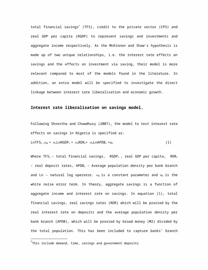
Following Shrestha and Chowdhury (2007), the model to test interest rate effects on savings in Nigeria is

specified as:

LnTFSt =0 + 1LnRGDPt + 2RDRt+ 3LnAPDBt +ut (1)

Where TFSt – total financial savings, RGDPt , real GDP per capita, RDRt – real deposit rates, APDBt –

Average population density per bank branch and Ln – natural log operator. 0 is a constant

parameter and ut is the white noise error term. In theory, aggregate savings is a function of

aggregate income and interest rate on savings. In equation (1), total financial savings, real savings rates

(RDR) which will be proxied by the real interest rate on deposits and the average population density per

bank branch (APDB), which will be proxied by broad money (M2) divided by the total population. This has

been included to capture banks’ branch proliferation. This can also be viewed as a relative measure of

financial deepening in the economy. The McKinnon-Shaw hypothesis argues that financial repression

stifles savings. Therefore only financial liberalisation will lead to higher savings, higher investment and

ultimately to accelerated economic growth in the economy. Interest rate can be viewed as the cost for

borrowing money or as the opportunity cost of lending money for a period of time. The real interest rate,

the rate adjusted for anticipated inflation, is thus vital for the supply and demand for financial resources.

The hypothesis further asserts that higher real interest rate also helps direct the funds to the most productive

7This include demand, time, savings and government deposits

enterprises and facilitate technological innovation leading to economic growth. It maintains that by paying

a rate of interest on financial assets that is significantly above the marginal efficiency of investment in

existing techniques, one can induce some entrepreneurs to disinvest from inferior processes to improved

technology and increased scale in other high yielding enterprises (McKinnon, 1973). The release of

resources from inferior means of production is as important as generating net new savings. Savings

provides the resources for investment in physical capital. Hence, it is an important determinant of economic

growth. Increased savings are also beneficial in reducing foreign dependence and insulating the economy

from external shocks (McKinnon, 1973).

Real per capita (RGDP) which is computed as real GDP divided by the total population is usually used to

indicate the size of individual income and rate of economic development of a country. In theory, given the

marginal propensity to save, the higher the income, the higher the amount of income saved. It is therefore

plausible to use it as an independent variable to investigate the effects of interest rate liberalisation on

savings. It is argued that as the number of bank branches increases, the banks are able to mobilise more

deposits and therefore the increased number of bank branches is viewed as having positive effect on the

total deposit mobilisation and hence total savings (Shrestha and Chowdhury 2007). According to

Chandrasekhar (2007), there is no reason to expect a linear and positive relationship between proliferation

of bank branches and increased financial savings. Branch proliferation and increased financial

intermediation have their uses when economies develop and become more complex, but they are not virtues

in themselves (Ibid). In all economies, the value of financial proliferation depends on its ability to increase

savings or deposits mobilisation, ease transactions, facilitate investment and direct financial resources to

the projects that yield the best social returns and ultimately lead to economic growth. However, despite the

elaborate and sometimes expensive branch proliferation in developing countries, there tends to be relatively

little savings mobilisation through these process of expansion (Ghosh, 2005). In equation (1), 0 represent

the constant whilst ut is the error term. Based on the theoretical and the empirical analysis above, the

coefficient 1 and 2 are expected to be positive. Like Shrestha and Chowdhury (2007), this paper expects

3 to be negative.

Interest rate liberalisation on investment model.

The other part of the liberalisation hypothesis postulated by McKinnon (1973) and

Shaw (1973) is the positive relationship between real interest rate and investment

through savings. In line with Shrestha and Chowdhury (2007), the model to test this

part, .i.e. the effects of interest rate liberalisation on investments through savings is specified as:

LnCPSt= β0 + β1LnTFSt+ β2RBLRt+ β3RRRt + β4RBCBt + et (2)

Where CPSt – investment (proxied by the volume of credit to the private sector), TFS t - savings (proxied

by the total financial savings), RBLRt – real bank lending rate, RRRt – real refinance rate (proxied by the

real discount rates), RBCBt – real borrowings from central bank and Ln – natural log operator. β 0 is a

constant parameter and et is the white noise error term. The McKinnon-Shaw hypothesis

argues that financial repression stifles economic growth as a result of controls on financial resources. They

argue that only liberalisation of the financial sector will lead to increase in savings which in turn lead to

increase in investment and hence economic growth. In equation (2), investment (CPS) is expressed as a

function of savings (TFS), real lending rate (RBLR), real refinance rate (RRR) and real borrowing from the

central bank (RBCB). The equation suggests that investment is determined by prior savings and the real

returns available on other assets. Theoretically, savings is equal to investments in equilibrium (Montiel,

1995). This is true in McKinnon’s world, as per his complementarity hypothesis. However, Shaw’s debt

intermediation hypothesis, assumes no prior savings and to cater for investment outside savings the real

borrowing from the central bank (RBCB) have been include in equation (2) to capture investments outside

savings. Credit to the private sector (CPS) as the ratio of total credit extended to the

private sector by the banks to the GDP, measures the level of activities and efficiency

of the financial intermediation. An increase in the financial resources, especially

credits, to the private sector is expected to increase private sector efficiency and

production and consequently lead to economic growth.

Theoretically, investment decisions are based on marginal benefit versus marginal cost process and it is

determined by the expected rate of return on the investment and the interest rate that must be paid to the

lender of the financial resources. An investment is therefore made if the expected rate of return is higher

than the interest rate. This would suggest that there is an inverse relationship between the interest rate on

lending and the expected rate of return on one hand and the quantity or level of investment demanded. In

equation (2), real lending rate (RBLR) and real refinance rate (RRR), which will be proxied by the discount

rate, have been included to represent interest rate on lending and expected rate of return respectively.

Haavelmo (1960) and Jorgenson (1963) show that increasing the interest rate reduces investment by raising

the cost of capital. However, Chetty (2007) investigating interest rate and investment, shows that this may

sometime not be the case as firms make irreversible investments with uncertain pay-offs. In this

environment, he argues, investment becomes a “backward-bending” function of the interest rates.

Furthermore, Eregha (2010) investigating interest rates and investment determinants in Nigeria, reveals that

variation in interest rates and higher rate on interest rate have a negative and significant influence on

investment decisions and demand for credit have negative influence on interest rate in the short run as well

as in the long run. In line with Shrestha and Chowdhury (2007) and the above analysis, the coefficients β1

andβ4 are expected to be positive but β2 and β3 are expected to be negative. Now let’s look at the effects

interest rate liberalisation on economic growth.

Interest rate liberalisation on economic growth model.

The gist of the McKinnon-Shaw hypothesis is that interest rate liberalisation promotes savings and

investment and ultimately leads to increase in economic growth. They argue that real interest rates

influence economic growth through their positive effects on savings and investment. The McKinnon and

Shaw hypothesis can be expressed in the form of Harrod-Domar growth model (Hussain, 1995). Thus:

g = z(S8/Y) = z(I/Y) (3)

8 This is total savings and not financial savings.

where g is the rate of growth of real output, z is the productivity of capital and (S/Y) is the ratio of domestic

savings to GDP when in equilibrium is equal to the ratio of domestic investment to GDP (i.e. I/Y).

Accordingly, given the productivity of capital, the growth rate should increase, the higher the ratio of

savings (investments) to GDP. Conversely, if the ratio of savings to GDP is given, the growth rate can be

increased by improving the efficacy of investments which will then raise the productivity of capital, z

(Hussain, 1995). The orthodox approach suggests that interest rate liberalisation will increase both the

savings and improve the efficiency of investments (Shaw 1973). Okuda (1990) points out that to do this, it

is important to promote investment that will support efficient production in the sectors of the economy with

the highest expectation of rapid economic growth (Hussain et al, 2002). Based on the above analysis, the

paper specifies a modified version of the growth model used by Beck et al (2000) and then by Fowowe

(2002) where the growth rate of GDP per capita is regressed on other financial sector indicators. Thus,

following Beck et al (2002) and Fowowe (2002), our economic growth model is specified as:

LnRGDPt= σ0 + σ1LnLt+ σ2LnKt+σ3FDIt +σ4LnCPSt + σ5FLIRt + et (4)

where RGDPt , real GDP per capita, FDIt – foreign direct investments, CPSt – investment (credit to the

private sector), FLIRt – interest rate liberalisation index and Ln – natural log operator. σ0 is a constant

parameter and et is the white noise error term. In equation (4), economic growth

(RGDP) is expressed as a function of real investment (CPS) which in turn is expressed

as a function of savings as in equation (2) as well as foreign investments (FDI).

According to McKinnon-Shaw hypothesis, liberalisation of interest rate leads to

increase in savings then increase in investments and ultimately leading to increase in

economic growth. Montiel (1995) using a simple aggregate production function

framework, shows that interest rate liberalisation can alter the economic growth rate

through three main channels. He identified these three channels as: (i) increase in

investment resulting from the increase in savings rate; (ii) improvement in the

efficiency of capital stock and (iii) improvement in the financial intermediation. These

are similar factors to that of the Harrod-Domar growth model explained above.

To improve the efficiency of capital requires human effort and this has been captured

by including capital stock (K) and a labour factor (L) in equation (4). In a closed

economy, savings will equal investments in equilibrium, however, Nigeria is an open

economy and hence to capture the effects of external investment, foreign direct

investment (FDI) have been included as a control variable. Foreign direct investments

are known to have positive effects on economic growth (Bengoa-Calvo, 2002). To

capture the improvement in the financial intermediation, an interest rate

liberalisation index (FLIR) has been included in equation (4). This is because

improvement in intermediation comes through policy changes which the index will

reflect. Based on the above analysis, all the coefficients, σ1, σ2, σ3 and σ4, are expected to

be positive.

The ARDL - bounds testing approach based on unrestricted error correction model (UECM) technique

involves two stages. The first stage is to estimate the ARDL model of interest by ordinary least squares

(OLS) in order to test for the existence of a long run relationship among the relevant variables. This is done

by construction an unrestricted error correction models (UECM) and then testing whether the lagged levels

of the variables in each of the equations are statistically significant or not. In other words, whether the null

hypothesis of no long term relationship is rejected or accepted. This is done by conducting a Wald test (F-

test version for bound testing methodology) for the joint significance of the lagged levels of the variables,

i.e. testing the null hypothesis against the alternative hypothesis. If the F-statistics is above the upper

critical value, the null hypothesis of no long run relationship can be rejected irrespective of the orders of

integration for the time series. Conversely, if the test statistics falls below the lower critical values then the

null hypothesis cannot be rejected. However, if the statistics falls between the upper and the lower critical

values, then result is inconclusive. In this case the asymptotic distribution of the Wald test (F- statistics) is

non-standard under the null hypothesis of no cointegration relation between the variables of interest,

irrespective whether the explanatory variables are purely I(0) or I(1).

Once the long run relationship or cointegration has been established, the second stage of the testing

involves the estimation of the long run coefficients (which represent the optimum order of the variables

after selection by AIC or SBC) and then estimate the associated error correction model in order to estimate

the adjustment coefficients of the error correction term (Masih et al, 2008). The short run effects therefore

will be captured by the coefficients of the first differenced variables in the UECM model. According to

Bahmani-Oskooee and Brooks (1999) the existence of a long term relationship derived from Equations 1, 2

and 4 do not necessarily imply that the estimated coefficients are stable. This suggests that there is the need

to perform series of tests diagnosis on the model established. This involves testing of the residuals (i.e.

homoscedasticity, non-serial correlation, etc.) as well as stability tests to ensure that the estimated model is

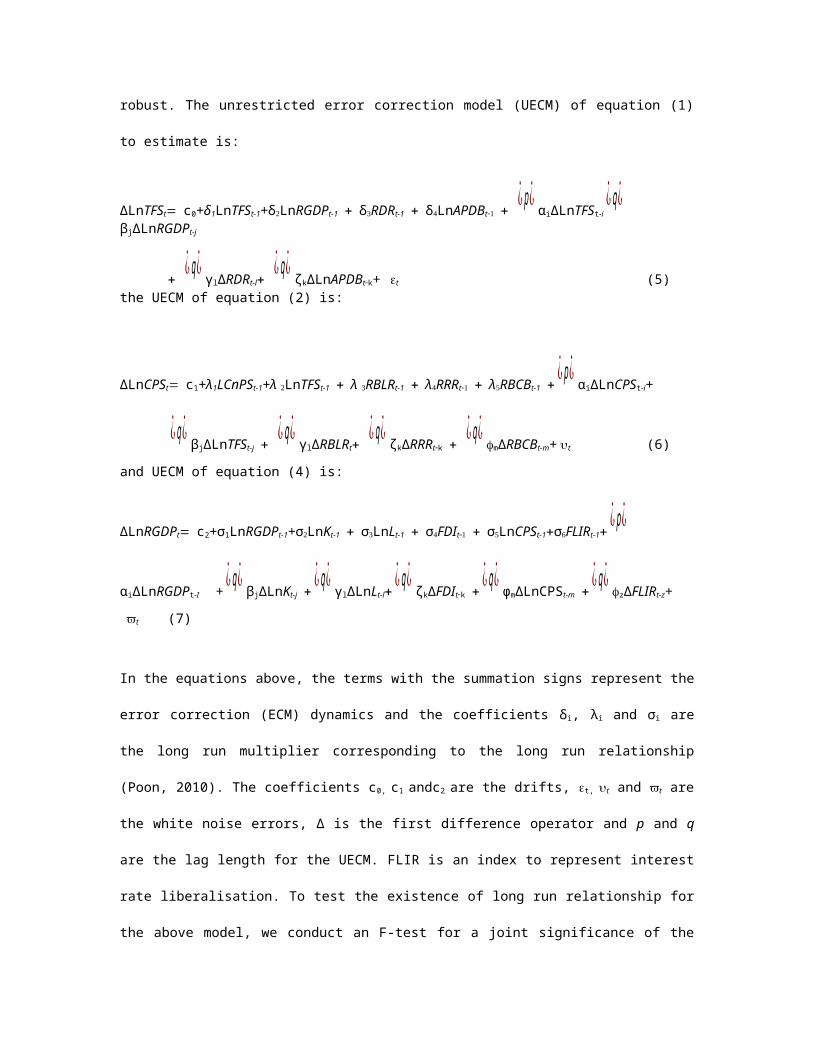
statistically robust. The unrestricted error correction model (UECM) of equation (1) to estimate is:

ΔLnTFStc0+δ1LnTFSt-1+δLnRGDPt-1δRDRt-1δLnAPDBt¿ p¿

αiΔLnTFSt-i¿ q¿

βjΔLnRGDPt-j

¿ q¿

γlΔRDRt-l¿ q¿

ζkΔLnAPDBtk+ t

(5)the UECM of equation (2) is:

ΔLnCPStc1+λ1LCnPSt-1+λLnTFSt-1λRBLRt-1λRRRtλRBCBt-1¿ p¿

αiΔLnCPSt-

i+

¿ q¿βjΔLnTFSt-j

¿ q¿γlΔRBLRt

¿ q¿ζkΔRRRtk

¿ q¿mΔRBCBt-m+ t

(6)and UECM of equation (4) is:

ΔLnRGDPtc2+σ1LnRGDPt-1+σLnKt-1σLnLt-1σFDItσLnCPSt-1σFLIRt-1¿ p¿

αiΔLnRGDPt-I +¿ q¿

βjΔLnKt-j¿ q¿

γlΔLnLt-l¿ q¿

ζkΔFDItk¿ q¿ϕmΔLnCPSt-m

¿ q¿zΔFLIRt-z+

t (7)

In the equations above, the terms with the summation signs represent the error correction (ECM) dynamics

and the coefficients δi, λi and σi are the long run multiplier corresponding to the long run relationship (Poon,

2010). The coefficients c0, c1 andc2 are the drifts, t, t and t are the white noise errors, Δ is the first

difference operator and p and q are the lag length for the UECM. FLIR is an index to

represent interest rate liberalisation. To test the existence of long run relationship for the above

model, we conduct an F-test for a joint significance of the coefficient of the lagged levels by using ordinary

least square (OLS). Thus, test the null hypotheses, HN : δ1 = δ2= δ3= δ4= 0, HN : λ1 = λ 2= λ 3= λ 4= λ 5= 0 and

HN : σ1 = σ2= σ3= σ4= σ5= σ6 = 0 which indicate no long run relationship against the alternative hypotheses,

HA : δ1 δ2 δ3 δ4 0, HA : λ1 λ2 λ 3 λ 4 λ5 0 and HA : σ1 σ2 σ3 σ4 σ5 σ6 0. The

functions which normalise the tests are denoted by FLnTFS (LnTFS| LnRGDP, RDR, LnAPDB), FLnCPS

(LnCPS| LnTFS, RBLR, RRR, RBCB) and FLnRGDP (LnRGDP| LnL, LnK, FDI, LnCPS, FLIR).

The general UECM model is tested downwards sequentially by dropping the statistically non-significant

first differenced variables for each of the equations to arrive at a “goodness of fit” models using general-to-

specific strategy (Poon, 2010). Once the cointegration relationships are established, the order of the ARDL

for the model is selected using Akaike information criteria (AIC) or Schwarz Bayesian Criteria (SBC). The

long run elasticities or coefficients can then be generated from UECM by using the estimated coefficients

of the one lagged independent variables, multiplied by a negative sign, and divided by the estimated

coefficient of the one lagged dependent variable (Bardsen, 1989). The short run coefficients are then

derived from the estimated coefficient of the first differenced variable in UECM models (Poon, 2010).

4.2 Empirical Analysis.

The bounds testing approach involves two stages. In the first stage, an arbitrary number of lags are imposed

on the first differenced variables then the F-test for joint significance is carried out to test for cointegration

among the relevant variables. However, according to Bahmani-Oskooee and Brooks (1999) as well as

Bahmani-Oskooee and Goswani (2004), the results of the F-test on this basis could be sensitive to the

choice of the lag length (Bahmani-Oskooee and Karacal, 2006). As a result, following Bahmani-Oskooee

and Karacal (2006), this paper first estimates the ARDL model then uses either Akaike Information

Criterion (AIC) or the Schwarz Bayesian Criterion (SBC) to select the optimum number of lags before

carrying out the F-test of joint significance at the optimum lags. Before the paper goes ahead with the

ARDL bounds testing, it will first test for the stationarity of all the variables that are going to be used in the

analysis to ensure that they are all in the order of I(0) or I(1) stationary so as to avoid spurious results

(Ouattara, 2004).

4.2.1 Unit root tests for variables.

The results of the Dickey-Fuller generalised least squares (DF-GLS) and the Phillips and Peron (PP) unit

root tests for Nigeria are reported in Tables 1 to 4 below. The DF-GLS lag length is selected automatically

by AIC whilst the PP truncation lag is selected automatically on the Newey-West bandwidth.

Table 1: DF-GLS unit root tests for the variables in levels.Variable No Trend Result Trend Result

LnAPDB

LnCPS

FDI

FLIR

LnK

LnL

LnRGDP

RBCB

RBLR

RDR

RRR

LnTFS

-0.680370

0.367708

-1.558110

0.846217

-0.933244

-3.400259***

-1.484503

-1.842932*

-3.906732***

-4.136936***

-4.061984***

-1.164602

N

N

N

N

N

S

N

S

S

S

S

N

-1.567795

-2.405547

-2.805986

-1.827261

-1.635655

-3.479230**

-2.115570

-2.900083*

-4.391699***

-4.406230***

-4.305378***

-1.489884

N

N

N

N

N

S

N

S

S

S

S

N

Notes: *, ** and *** denote the rejection of the null hypothesis at 10%, 5% and 1% significant levels respectively. S = Stationary and N = Non-stationary. Ln is the natural log operator. The log of one plus the inflation rates were used to diminish the impact of some outlier observations.

Table 2: DF-GLS unit root tests for the variables in first differences.Variable No Trend Result Trend Result

∆LnAPDB

∆LnCPS

-4.826463***

-4.258093***

S

S

-5.211895***

-4.444681***

S

S

Variable No Trend Result Trend Result

∆FDI

∆FLIR

∆LnK

∆LnRGDP

∆LnTFS

-10.64796***

-6.114258***

-4.596922***

-2.742804***

-1.858083*

S

S

S

S

S

-10.43796***

-6.528555***

-5.025509***

-4.06934***

-4.948947***

S

S

S

S

S

Notes: S = Stationary and N = Non-stationary. ∆ is the difference operator and L is the log operator. *, ** and *** denote the rejection of the null hypothesis at 10%, 5% and 1% significant levels respectively.

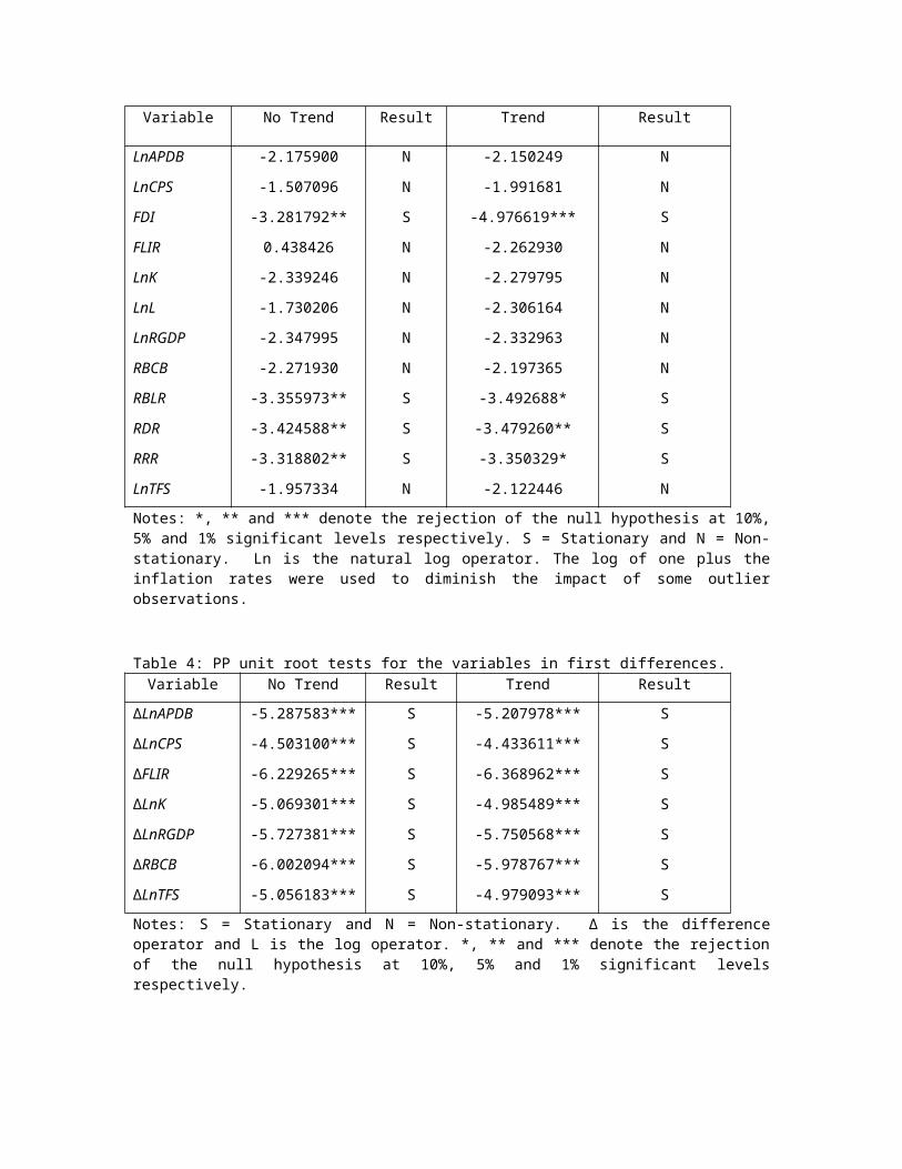
Table 3: PP unit root tests for the variables in levels.Variable No Trend Result Trend Result

LnAPDB

LnCPS

FDI

FLIR

LnK

LnL

LnRGDP

RBCB

RBLR

RDR

RRR

LnTFS

-2.175900

-1.507096

-3.281792**

0.438426

-2.339246

-1.730206

-2.347995

-2.271930

-3.355973**

-3.424588**

-3.318802**

-1.957334

N

N

S

N

N

N

N

N

S

S

S

N

-2.150249

-1.991681

-4.976619***

-2.262930

-2.279795

-2.306164

-2.332963

-2.197365

-3.492688*

-3.479260**

-3.350329*

-2.122446

N

N

S

N

N

N

N

N

S

S

S

N

Notes: *, ** and *** denote the rejection of the null hypothesis at 10%, 5% and 1% significant levels respectively. S = Stationary and N = Non-stationary. Ln is the natural log operator. The log of one plus the inflation rates were used to diminish the impact of some outlier observations.

Table 4: PP unit root tests for the variables in first differences.Variable No Trend Result Trend Result

∆LnAPDB

∆LnCPS

∆FLIR

∆LnK

∆LnRGDP

∆RBCB

∆LnTFS

-5.287583***

-4.503100***

-6.229265***

-5.069301***

-5.727381***

-6.002094***

-5.056183***

S

S

S

S

S

S

S

-5.207978***

-4.433611***

-6.368962***

-4.985489***

-5.750568***

-5.978767***

-4.979093***

S

S

S

S

S

S

S

Notes: S = Stationary and N = Non-stationary. ∆ is the difference operator and L is the log operator. *, ** and *** denote the rejection of the null hypothesis at 10%, 5% and 1% significant levels respectively.

As can be seen from Tables 1 to 4 all the variables are either I(0) or I(1) using both tests for Nigeria. The

paper therefore rejects the null hypothesis that the variables have unit roots on the basis of Akaike

Information Criteria (AIC) and the Newey-West bandwidth as well as the serial correlation diagnostic tests

from the stationarity regression results. Hence, the paper concludes that there are no I(2) variables in the

case of Nigeria.

Testing for the McKinnon-Shaw hypothesis and the effects of interest rate liberalisation on economic growth.

The results from the stationarity tests indicate that the savings model can be implemented as an ARDL

model using bounds testing approach as in Pesaran et al (2001). The calculated F-statistics FLnTFS (LnTFS|

LnRGDP, RDR, LnAPDB) = 6.8207 at an optimum lag of 2. This is higher than the upper bound critical

value of 5.23 at 1% significant level (Table 5)

Table 5: Modelling of Savings Function - Bounds F-test for cointegration.Dependent variable Function F-test statistics

LnTFS FLnTFS (LnTFS| LnRGDP, RDR, LnAPDB) 6.8207***

Asymptotic Critical Values

Pesaran et al (2001),

p.301, Table CI(iv) Case

IV

1% 5% 10%

I(0) I(1) I(0) I(1) I(0) I(0)

4.30 5.23 3.38 4.23 2.97 3.74

Note: *** denotes statistical significant at the 1% level.

Thus, the null hypothesis of non-existence of cointegration among the variables is rejected. This implies

that there is a long run cointegration relationship amongst the variables when the model is normalised on

real total financial savings (LnTFS) in Nigeria. In determining the optimum lag, the paper has followed

Bahmani-Oskooee and Brooks (1999), Bahmani-Oskooee and Goswani (2004) and Bahmani-Oskooee and

Karacal (2006) who argue that the result of the F-statistics could be sensitive to the choice of the lag length.

Therefore, the paper first estimates the ARDL model then uses AIC or SBC to select the optimum lag. The

SBC based ARDL (2, 0, 0, 2) model was selected because it has a lower mean prediction errors as well as a

lower estimated standard error than the AIC based model (Shrestha and Chowdhury, 2007). The long run

results of the selected model are reported in Table 6 below.

Table 6: Modelling of Savings Function - Results of ARDL (2, 0, 0, 2) long run model selected on SBC.Regressor Co-efficient Standard Error T-Ratio Prob.

C

LnRGDP

RDR

LnAPDB

12.1833

-2.3999

0.070385

1.1211

17.1629

2.7643

0.041745

0.27899

0.70986

-0.86819

1.6861

4.0184

0.483

0.392

0.100

0.000

Notes: Dependent variable: LnTFS

The long run model result (Table 6) reveal that the real interest rate on deposit (RDR) and average

population per bank (LnAPDB) in Nigeria are the key determinants of financial savings. The coefficient of

0.070385 for RDR is positive as expected and is statistically significant at the 10% significant level. It

suggests that in the long run, an increase of 1% in the real deposit rate is associated with an increase of

$1.18 billion in total financial savings in Nigeria9. The results also show that real GDP per capita

(LnRGDP) has statistically insignificant effect on economics growth in Nigeria. Furthermore, the sign is

not what was expected. Also, the coefficient of the Average population per bank in Nigeria is significant at

1% level, but the sign is not what was expected. The positive sign for this coefficient may suggest that bank

branch proliferation leads to increase in savings mobilisation in Nigeria. This is contrary to Ghosh (2005)

and Chandrasekhar (2007). The short run dynamics of the model are shown in Table 7.

Table 7: Modelling of Savings Function - Results of ARDL (2, 0, 0, 2) ECM model selected on SBC.Regressor Co-efficient Standard Error T-Ratio Prob.

∆LnTFS-2 -0.37341 0.14789 -2.5249 0.017

∆LnRGDP-1 -0.14829 0.14627 -1.0138 0.319

∆RDR-1 0.0043490 0.0012554 3.4643 0.002

∆LnAPDB-1 1.0104 0.040118 25.1870 0.000

∆LnAPDB-2 0.44289 0.14752 3.0021 0.005

ecm(-1) -0.061788 0.032703 -1.7306 0.093

9LnTFS is in a log form while RDR is in the level form. An anti-log of the coefficient of RDR, which is 0.070385, is 1.18.

Regressor Co-efficient Standard Error T-Ratio Prob.

R-Squared 0.97114 R-Bar-Squared 0.96441S.E. of Regression 0.068257 F-Stat. F(6,31) 168.26501[0.000]Residual Sum of Squares 0.13977 DW-statistic 1.9901Akaike Info. Criterion 44.5819 Schwarz Bayesian Criterion 38.0315Notes: Dependent variable: ∆LnTFS-1

Table 7 indicates that the coefficients of ∆LnTFS-2, ∆RDR-1, ∆LnAPDB-1 and ∆LnAPDB-2 are all

statistically significant but ∆LnTFS-2 has negative impact. This implies that real deposit rate and average

population per bank have some significant impact in the long run on total financial savings in Nigeria

(Table 6) as well as short run impacts. The table also shows that ∆LnRGDP-1 has negative and insignificant

on total financial savings in the short run. The coefficient of ECM(-1) is found to be statistically significant

at 10% level. This confirms the existence of a long run relationship between the variables. The coefficient

of ECM term is -0.061788, which suggests a very slow rate of adjustment process. This implies that the

disequilibrium occurring due to a shock is totally corrected in about 16 years and 2 months at a rate of 6.2%

per annum.

Table 8: Modelling of Savings Function - ARDL-VECM model diagnostics tests.LM Test Statistics Results

Serial Correlation:CHSQ(1)

Functional Form: CHSQ(1)

Normality: CHSQ(2)

Hetroscedasticity: CHSQ(1)

0.064171[0.800]

0.95114[0.329]

0.22452[0.894]

0.0084663[0.927]

Finally, the regression for the underlying ARDL model fits very well at R square = 99.5% and also it passes

the diagnostic tests against serial correlation, Functional Form, Normality and Hetroscedasticity as shown

in Table 8. Also, an inspection of the cumulative sum (CUSUM) and the cumulative sum of squares

(CUSUMSQ) graphs (Figures 1 and 2) from the recursive estimation of the model reveals there is stability

and there is no systematic change detected in the coefficient at 5% significant level over the sample

period.The above findings show that the real deposit rate plays a positive and significant role in increasing

the total financial savings in Nigeria. These results clearly support the first part of the McKinnon-Shaw

hypothesis in Nigeria. Now let us look at the second part of the McKinnon-Shaw hypothesis in Nigeria.

The results from the stationarity tests indicate that the investment model can be implemented as an ARDL

model using bounds testing approach as in Pesaran et al (2001). The calculated F-statistics F LnCPS (LnCPS|

LnTFS, RBLR, RRR) = 5.0970 at an optimum lag of 5. This is higher than the upper bound critical value of

4.23 at 5% significant level (Table 9).

Table 9: Modelling of Investment Function - Bounds F-test for cointegration.Dependent variable Function F-test statistics

LnCPS FLnCPS (LnCPS| LnTFS, RBLR, RRR) 5.0970**




IV

1% 5% 10%

I(0) I(1) I(0) I(1) I(0) I(0)

4.30 5.23 3.38 4.23 2.97 3.74

Note: ** denotes statistical significant at the 5% level.



real credit to the private sector (LnCPS) in Nigeria. The paper has followed Bahmani-Oskooee and Brooks

(1999), Bahmani-Oskooee and Goswani (2004) and Bahmani-Oskooee and Karacal (2006) in determining

the optimum lag. Thus, the paper first estimates the ARDL model then uses AIC or SBC to select the

optimum lag. The SBC based ARDL (2, 1, 5, 5) model was selected because it has a lower mean prediction

errors as well as a lower estimated standard error than the AIC based model (Shrestha and Chowdhury,

2007). The real borrowing from central bank (RBCB) variable has been excluded as it is statistically

insignificant. The long run results of the selected model are reported in Table 10 below.

Table 10: Modelling of Investment Function - Results of ARDL (2, 1, 5, 5) long run model selected on SBC.Regressor Co-efficient Standard Error T-Ratio Prob.

C

LnTFS

RBLR

RRR

-0.34608

1.1317

0.16975

-0.17718

0.19919

0.061857

0.032153

0.036367

-1.7375

18.2964

5.2795

-4.8720

0.099

0.000

0.000

0.000

Notes: Dependent variable: LnCPS

The long run results reported in Table 10 show that the total financial savings is the main determinant of

credit to the private sector (a proxy for investment) in Nigeria. The coefficient of total financial savings

(LnTFS) of 1.1317 is positive, as expected and statistically significant at 1% level. This implies that an

increase in the total financial savings by $1billion would lead to an increase in credit to the private sector

by $1.1317 billion in the long run. The real bank lending rate (RBLR) is found to be positive and

statistically significant at 1%. This may suggest that the lending rate of banks does have impact on the

volume of bank credit to the private sector in Nigeria. The real refinance rates (discount rates) also were

found to have the expected sign and statistically significant at 1% in the long run. The short run dynamics

of the model are shown in Table 11.

Table 11: Modelling of Investment Function - Results of ARDL (2, 1, 5, 5) ECM model selected on SBC.Regressor Co-efficient Standard Error T-Ratio Prob.

∆LnCPS-2 -0.12485 0.067652 -1.8455 0.079

∆LnTFS-1 0.87231 0.054358 16.0474 0.000

∆RBLR-1 0.0032875 0.013345 0.24635 0.808

∆RBLR-2 -0.067790 0.019818 -3.4206 0.003

∆RBLR-3 -0.036403 0.018664 -1.9505 0.065

∆RBLR-4 -0.065860 0.018497 -3.5606 0.002

∆RBLR-5 -0.059810 0.014107 -4.2397 0.000

∆RRR-1 -0.0057082 0.013612 -0.41934 0.679

∆RRR-2 0.068574 0.019723 3.4769 0.002

∆RRR-3 0.036719 0.018716 1.9618 0.063

∆RRR-4 0.061747 0.018862 3.2735 0.004

∆RRR-5 0.061763 0.014496 4.2609 0.000

ecm(-1) -0.54693 0.13558 -4.0341 0.001

R-Squared 0.96779 R-Bar-Squared 0.93917S.E. of Regression 0.090477 F-Stat. F(13,21) 41.6089[0.000]Residual Sum of Squares 0.14735 DW-statistic 2.3428Akaike Info. Criterion 29.0673 Schwarz Bayesian Criterion 15.8468Notes: Dependent variable: ∆LnCPS-1

Table 9 reports the short run dynamics of the second part of the McKinnon-Shaw hypothesis. The

coefficient of ECM(-1) is -0.54693 and statistically significant at 1% level. This implies that the

disequilibrium occurring due to a shock to the volume of credit advanced by the banks to the private sector

is totally corrected in about 1 year 10 months at a rate of about 54.69% per annum. The ECM result also

shows that a change in the total financial savings is also associated with a positive change in credit to the

private sector (∆LnCPS-1) and is very significant at 1% level. However, both the coefficients of ∆RRR -1

and ∆RBLR-1 are statistically insignificant and show that changes in the real refinance rates (discount rates)

and real borrowing rates have insignificant impact on the change in credit to the private sector.

Table 12: Modelling of Investment Function - ARDL-VECM model diagnostic tests.LM Test Statistics Results

Serial Correlation: CHSQ(1)


Normality: CHSQ(2)


1.7562[0.185]

0.081192[0.776]

0.36393[0.834]

0.50540[0.477]

Finally, the regression for the underlying ARDL model fits very well at R square = 99.35% and also it

passes all the diagnostic tests against serial correlation, functional form, Normality and Hetroscedasticity as

shown in Table 12. Furthermore, an inspection of the cumulative sum (CUSUM) and the cumulative sum

of squares (CUSUMSQ) graphs (Figures 3 and 4) from the recursive estimation of the model reveals there

is stability and there is no systematic change detected in the coefficient at 5% significant level over the

sample period. The above findings show that the total financial savings play a positive and significant role

in increasing the volume of credit that the banks extend to the private sector (proxy for investments) in

Nigeria. These results clearly support the second part of the McKinnon-Shaw hypothesis in Nigeria. We

now test for the effects of interest rate liberalisation on the economic growth in the Nigerian economy.

The results from the stationarity tests indicate that the economic growth model can be implemented as an

ARDL model using bounds testing approach as in Pesaran et al (2001). The calculated F-statistics FLnRGDP

(LnRGDP| LnL, LnK, FDI, LnCPS, FLIR) = 4.6485 at an optimum lag of 4. This is higher than the upper

bound critical value of 4.63 at 1% significant level (Table 13).

Table 13: Modelling of Economic Growth Function - Bounds F-test for cointegration.Dependent variable Function F-test statistics

LnY = LnRGDP FLnRGDP (LnRGDP| LnL, LnK, FDI, LnCPS, FLIR) 4.6485***




IV

1% 5% 10%

I(0) I(1) I(0) I(1) I(0) I(0)

3.50 4.63 2.81 3.76 2.49 3.38

Note: *** denotes statistical significant at the 1% level.



real GDP per capita in Nigeria. The optimum lag has been determined as in Bahmani-Oskooee and Brooks

(1999), Bahmani-Oskooee and Goswani (2004) and Bahmani-Oskooee and Karacal (2006). Thus, the paper

first estimates the ARDL model then uses AIC or SBC to select the optimum lag. The SBC based ARDL

(4, 0, 1, 3, 0, 0) model was selected because it has a lower mean prediction errors as well as a lower

estimated standard error than the AIC based model (Shrestha and Chowdhury, 2007). The long run results

of the selected model are reported in Table 14 below.

Table 14: Modelling of Economic Growth Function - Results of ARDL (4, 0, 1, 3, 0, 0) long run model selected on SBC.Regressor Co-efficient Standard Error T-Ratio Prob.

C

LnK

LnL

FDI

LnCPS

FLIR

-18.7164

0.062332

7.0675

0.048008

-0.085445

0.055067

5.74486

0.025968

1.6637

0.014753

0.033346

0.017913

-3.2558

2.4003

4.2481

3.2542

-2.5624

3.0741

0.004

0.025

0.000

0.004

0.018

0.006

Notes: Dependent variable: LnRGDP = LnY

The long run results reported in Table 14 show that the interest rate liberalisation has a positive long run

effect on the economic growth in Nigeria. The coefficient of the interest rate liberalisation index is positive

as expected as well as statistically significant. This suggest that 1% increase in the interest rate

liberalisation index, a proxy for policy changes, leads to an increase of 0.06% in economic growth. In fact,

all the other variables included in the model, Labour (LnL), Capital Stock (LnK) and Foreign Direct

Investments (FDI) are all statistically significant in Nigeria. This supports previous studies [e.g. Roubini

and Sala-i-Martin (1992) and Charlier and Ogun (2002) to mention a few] which found long run

relationship between economic growth and interest rate liberalisation. It is also observed that the

coefficient of credit to the private sector (LnCPS) has a negative sign contrary to expectation. Obamuyi

(2009) also finds a negatives relationship between credits to the private sector and economic growth in

Nigeria. He attributes this to the fact that private sector credits are mainly used to buying and selling

instead of productive activities. The coefficient may suggest that 1% increase in the volume of credit to the

private sector in Nigeria leads to a reduction of 0.09% in economic growth. The short run dynamics of the

model are shown in Table 15.

Table 15: Modelling of Economic Growth Function - Results of ARDL (4, 0, 1, 3, 0, 0) ECM model selected on SBC.Regressor Co-efficient Standard Error T-Ratio Prob.

∆LnRGDP-2 0.17318 0.17257 1.0036 0.326

∆LnRGDP-3 0.12008 0.13631 088092 0.387

∆LnRGDP-4 057774 0.11457 5.0426 0.000

∆LnK-1 0.039101 0.020196 1.9361 0.065

∆LnL-1 -3.6885 2.0270 -1.8197 0.081

∆FDI-1 0.0027760 0.0033115 0.83828 0.410

∆FDI-2 -0.017328 0.0058547 -2.9597 0.007

∆FDI-3 -0.0085091 0.0043433 -1.9591 0.062

∆LnCPS-1 -0.053600 0.017677 -3.0321 0.006

∆FLIR-1 0.034544 0.0074544 4.6340 0.000

ecm(-1) -0.62731 0.16657 -3.7661 0.001

R-Squared 0 .79898 R-Bar-Squared 0.68020S.E. of Regression 0.030301 F-Stat. F(11,21) 7.9493[0.000]Residual Sum of Squares 0.020199 DW-statistic 2.1509Akaike Info. Criterion 69.6599 Schwarz Bayesian Criterion 58.5753

Notes: Dependent variable: ∆LnRGDP-1 = ∆LnY-1

Table 15 reports the short run dynamics of the relationship between interest rate liberalisation and

economic growth. The coefficient of ECM(-1) is -0.62731 and statistically significant. This implies that the

disequilibrium occurring due to a shock to economic growth is totally corrected in about 1 year 7 months at

a rate of about 62.73% per annum. This confirms that there is a long run relationship between interest rate

liberalisation and economic growth in Nigeria. The ECM results however, show that a change in Labour is

also associated with a negative change in economic growth (∆LnRGDP-1) and is very significant at 10%

level. Also, the coefficient of ∆LnK-1 shows that a change in the capital stock is positively associated with

the change in economic growth but statistically significant at 10% level. Furthermore, the coefficient of the

change in the foreign direct investments (∆FDI-1) is positive but statistically insignificant. However, the

coefficient of ∆FDI-2, ∆FDI-3, and ∆LnCPS-1 are all negative and statistically significant. These three

coefficients may suggest that the bulk of the credit extended to the private sector by the banks and other

financial institutions goes into the import business (mostly buying and selling of imported finished

consumer goods) rather than production for domestic consumption in the real economy.

Table 16: Modelling of Economic Growth Function - ARDL-VECM model diagnostic tests.LM Test Statistics Results

Serial Correlation: CHSQ(1)


Normality: CHSQ(2)


0.62719[0.428]

2.4138[0.120]

0.60238[0.740]

0.48788[0.485]

Finally, the regression for the underlying ARDL model fits very well at R square = 96.06% and also it

passes all the diagnostic tests against serial correlation, functional form, Normality and Hetroscedasticity as

shown in Table 16. Also, an inspection of the cumulative sum (CUSUM) and the cumulative sum of

squares (CUSUMSQ) graphs (Figures 5 and 6) from the recursive estimation of the model reveals there is

stability and there is no systematic change detected in the coefficient at 5% significant level over the

sample period.

5 Conclusion

The main objective of this paper is to empirically examine and investigate the impact of interest rate

liberalisation policies on economic growth in Nigeria. The paper employs the ARDL bounds testing

approach and unrestricted error correction model (UECM) to cointegration analysis popularised by Pesaran

et al (2001) to establish the long run relationship between the relevant time series variables. It also applies a

multi-dimensional financial liberalisation index constructed from a number of financial liberalisation policy

measures implemented as a result of the interest rate liberalisation process in Nigeria.

The unit root tests employed suggest that, all the variables were found to be either I(0) or I(1) stationary.

Also, all the dependent variables were found to be cointegrated with the independent variables. This means

that long run relationships between the variables of interest were established. The empirical findings show

that the effect of interest rate liberalisation policies on economic growth in Nigeria is significant and

positive. The results from Nigeria do support the McKinnon-Shaw hypothesis, i.e. in the long run; interest

rate liberalisation will ultimately lead to rapid economic growth. The empirical findings also show that

interest rate liberalisation polices together with increase in the productivity of labour, increase in capital

stock and increase in foreign direct investments influence economic growth in Nigeria.

The policy implication arising out of the empirical findings is that the interest rate liberalisation policies

have been supportive but more needs to be done by the authorities in Nigeria to realise its full potential

effects on economic growth. These can be done by increasing financial deepening and the removal of

bottlenecks in the financial sectors of the economy. Also, by improving the effectiveness of credit to

private sector, efficient credit evaluation, public sector surveillance and abiding by stringent accounting

standards and auditing best practices, as well as adopting proper legal framework to help shape the

financial deepening process.

Figure 1: Plot of CUSUM for coefficients stability for ECM model (equation 5).

-20

-10

0

10

20

1971 1981 1991 2001 2008The straight lines represent critical bounds at 5% significance level

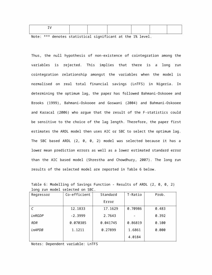
Figure 2: Plot of CUSUMSQ for coefficients stability for ECM model (equation 5).

-0.4

-0.2

0.0

0.2

0.4

0.6

0.8

1.0

1.2

1.4



-20

-10

0

10

20



-0.4

-0.2

0.0

0.2

0.4

0.6

0.8

1.0

1.2

1.4



-20

-10

0

10

20



-0.4

-0.2

0.0

0.2

0.4

0.6

0.8

1.0

1.2

1.4


References

Adebiyi, MA. 2005. Broad money demand, financial liberalisation and currency substitution in Nigeria. 8th

Capital Markets Conference: Indian Institute of capital Markets. India.

Bahmani-Oskooee, M and Karacal, M. 2006. The demand for money in Turkey and currency substitution, Applied Economics Letter, Vol. 13 (10): 635 – 642.

Bahmani-Oskooee, M and Brooks, TJ. 1999. Bilateral J-curve between U.S and her trading partners, Weltwirtschaftliches Archiv, Vol. 135: 156 – 165.

Bahmani-Oskooee, M and Goswami, G. 2004.Exchange rate sensitivity of Japans bilateral trade flow, Japan and the World Economy, Vol. 16: 1– 15.

Bardsen, G. 1989. Estimation of Long-Run Coefficients in Error Correction Models, Oxford Bulletin of Economics and Statistics, Vol: 51: 345-350.

Central Bank of Nigeria. 2009. Section A - Financial Statistics, Annual Statistical Bulletin, various issues.

Dickey, D and Fuller, W. 1979. Distribution of the Estimators for Autoregressive Time Series with a Unit Root, Journal of the American Statistical Association, 74, No. 1.

Fowowe, B. 2002. Financial liberalisation policies and Economic growth: Panel Data Evidence from Sub-Saharan Africa. African Econometrics Society Conference in 2008 (www.africametrics.org/documents/conference/2008).

Galbis, V. 1977. Financial intermediation and economic growth in less-developed countries: A theoretical approach. Journal of Development Economics, Vol. 13: 58-72.

Gibson, HD and Tsakalotos, E. 1994. The scope and limits of financial liberalisation in developing countries: A critical survey, Journal of Development Studies, pp: 578-628.

Goldsmith, RW. 1969. Financial structure and development. New Haven: Yale University Press.

Grabel, I. 1995. Speculation-led economic development: A post-Keynesian interpretation of financial liberalisation programmes in the Third World, International Review of Applied Economics,Vol. 9: 127-149.

Grabel, I. 1994. The political economy of theories of “optimal” financial repression: A critique, Review of Radical Political Economics, pp: 47-55.

International Monetary Fund (IMF). 2009. International Financial Statistics Yearbook,various issues to 2009, Washington DC.

Kapur, BK. 1983. Optimal financial and foreign-exchange liberalisation of less-developed country, Quarterly Journal of Economics, Vol.98:41-62

Kapur, BK. 1976. Alternative Stabilisation policies for Less Developed Countries, Journal of Political Economy, Vol. 84 (4): 777-795.

Kapur, BK. 1978. Alternative stabilisation policies for less-developed economies, Journal of Political Economy, Vol.84:777-95

Mathieson, DJ. 1979). Financial Reform and Capital Flows in a Developing Economy, IMF Staff Papers, Vol. 26 (3): 450-489.

Matheison, DJ. 1980. Financial reform and stabilisation policy in a Developing Economy, Journal of Development Economics, Vol.7: 359-95.

McKinnon, RI. 1973. Money and capital in Economic development. Washington DC: Brookings Institution.

Owusu, EL. 2011. Financial liberalisation and sustainable economic growth in primary commodity exporter countries (PCECs).PhD Thesis, University of South Africa (UNISA), Pretoria, South Africa.

Perron P. 1997. Further Evidence on Breaking Trend Functions in MacroeconomicVariables.Journal of Econometrics; Vol.80: 355-385.

Pesaran MH and Pesaran B. 1997.Working with Microfit 4.0: Interactive Econometric Analysis. Oxford, Oxford University Press.

Pesaran MH and Smith RP. 1998. Structural Analysis of Cointegrating VARs. Journal of Economic Survey; Vol.12: 471-505.

Pesaran MH and Shin Y. 1999. An Autoregressive Distributed Lag Modelling Approach to Cointegration Analysis. In S. Strom, A. Holly and P. Diamond (Eds.), Econometrics and Economic Theory in the 20th Century: The Ragner Frisch Centennial Symposium. Cambridge, Cambridge University Press. Available at: www.econ.cam.ac.uk/faculty/pesaran/ADL.pdf.

Pesaran, MH, Shin, Y and Smith RJ. 2001. Bounds Testing Approaches to the analysis of level relationships, Journal of Applied Econometrics, Vol.16:289-326.

Pesaran MH and Pesaran B. 2009.Working with Microfit 5.0: Interactive Econometric Analysis. Oxford, Oxford University Press.

Phillips PCB and Perron P. 1988.Testing for a Unit Root in Time Series Regression. Biometrica; Vol.75: 335-346.

Poon, W-C. 2010. A monetary policy rule: The augmented Monetary Conditions Index for Philippines using UECM and bounds tests, Discussion Paper 04/10, Issn 1441-5429, Monash University, Department of Economics.

Roubini, N and Sala-i-Martin, X. 1992. Financial Repression and EconomicGrowth, Journal of Development Economics; Vol.39(1): 5-30.

Shaw, ES. 1973. Financial deepening in economic development. New York: Oxford University Press.

Shrestha, MB and Chowdhury, K. 2007. Testing financial liberalisation hypothesis with ARDL modelling approach, Journal of Applied Financial Economics, Vol.17:1529-1540.

Taylor, L. 1983. Structuralist Macroeconomics: Applicable models for the Third World. New York: Basic Books.

Tobin, J. 1965. Money and Economic Growth, Econometrica; Vol. 33(4): 671-684.

Van Wijnbergen, S. 1983. Interest rate management in LDCs. Journal of Monetary Economics, Vol.12: 443-52.

World Bank. 1987. World Development Report. New York: Oxford University Press.

World Bank. 2009. World Development Report, various issues to 2009, Washington DC.

World Bank. 2009. African Development indicators, various issues to 2009, Washington DC

Documents

FINANCIAL LIBERALISATION - Journal€¦ · Web view), Dutt (1990) and Burkett and Dutt (1991) Using Tobin’s portfolio framework for household, thus household choice of investments