Department Socioeconomics

Financial Investment Constraints. A Panel

Threshold Application to German Firm

Level Data.

Artur Tarassow

DEP (Socioeconomics) Discussion Papers

Macroeconomics and Finance Series

5/2014

First version: September 2014

Revised version: August 2015

Hamburg, 2014

Financial Investment Constraints in Germany. A Panel

Threshold Application to Firm Level Data.

Artur Tarassow∗

Universität Hamburg

First Version: September 2014

Revised Version: September 2015

Abstract

This article tests the hypothesis that financial supply-side shifts help to explain the low-

investment climate of private firms in Germany. The core contention is that a firm’s financial

position contributes to its access to external finance on credit markets. Special emphasis is

put on small and medium-sized firms as these are assumed to face more restrictive access to

external sources of funds. The application of a non-linear panel threshold model allows us

to group firms endogenously according to their financial position. As potential threshold

variables nine different balance sheet indicators are used. The results reveal a positive

relationship between cash flows and fixed capital accumulation. Additional nonlinearity

suggests that financially fragile firms rely more heavily on retained earnings. In contrast to

frequent assumptions, firm size does not seem to be a relevant grouping variable in general

with the only exception being micro firms for which the probability to fall into a financially

constrained regime is higher compared to other companies.

JEL Classifications: A10, C23, D24, E22, E30, G31

Key Words: Firm investment, Balance sheet, Financial frictions, Credit rationing, SME,

Non-linear panel

∗Corresponding author, e-mail:artur.tarassow@wiso.uni-hamburg.de. I am grateful to Ingrid Größl, StevenFazzari, Ulrich Fritsche, Roberta Colavecchio, Jan-Oliver Menz, Stefan Schäfer, Nadja König, Annemarie Paul,Eva Arnold and participants at the 2013 IMK conference in Berlin as well as 2014 at the 8th InternationalConference on Computational and Financial Econometrics in Pisa for helpful comments and discussions. Thisarticle is part of my PhD dissertation project. Any remaining errors or omissions are strictly my own.

1

1 Introduction

Private investment growth has received much attention in recent years as a consequence of the

observed low growth in advanced economies since the outbreak of the recent great financial crisis

(GFC henceforth) in 2008 (IMF, 2015, Ch. 4).1 Different contributing factors of the sharp

recent downturn in investments are discussed, ranging from increased economic and political

uncertainty delaying investment decisions, over a slowdown in aggregate demand resulting in a

decline in expected profits, to an increase in financial constraints caused by a crash on credit

markets (IMF, 2015, Ch. 4). However, the persistently low fixed private investment rates realized

in Germany are not intuitive on a first glance as average bank lending rates are low, German firms

have increased their capital base on average during the past years, measures of credit constraints

have come down considerably since 2010, and energy prices are on historical lows. We argue

that the weak private investment dynamics observed on the aggregate level can be traced back

to financial frictions on the microeconomic level, in particular leveraged enterprises face. This

is in line with recent arguments made by the ECB that the weak recovery is mainly caused by

financial constraints stemming from the supply side on credit markets (ECB, 2013).

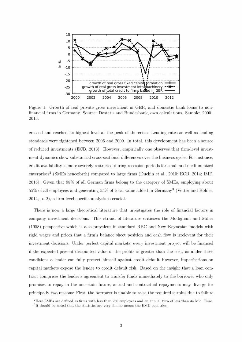
First evidence of an empirical relationship between private fixed investments and credit pro-

vided to non-financial firms operating in Germany, is displayed in Figure 1. Between 2000 and

2012 the annual average growth rates of real gross fixed capital formation and real gross invest-

ment into machinery are 0.28% and 1.06%, respectively. After a temporary increase in 2005,

private investments sharply collapsed as a result of the GFC. Between 2008 and 2009 real gross

fixed capital formation dropped by almost 15% and real gross investment into machinery even

by 25%. Throughout the whole period, low private investment rates were coupled with slow

credit growth to non-financial firms (around 2.3% on average). During the GFC, overall credit

growth remained still positive (except in 2010 when the growth rate was about −2.5%) but at

a decreasing rate. It should also be mentioned that according to Lenger and Ernstberger (2011)

some firms in Germany already faced credit constraints between 2000 and 2006 which helps to

explain the low investment climate since the early 2000s.

Additional evidence comes from recent ECB bank lending surveys, which indicate that ham-

pered access of non-financial firms to external finance has intensified the weak recovery since

2008. Supply-side driven financial frictions have tightened as banks’ perceptions of risk in-

1Monetary policy decision makers are interested in investment dynamics as the efficacy of transmission mech-anisms of monetary operations and its propagation effects on the business cycle crucially depend on the under-standings of the determinants of firm-level investments. Furthermore, the issue of capital accumulation is alsoclosely related to growth and innovation aspects, market competition; and hence a key variable for industrialpolicy decisions.

2

-30-25-20-15-10

-5 0 5

10 15

2000 2002 2004 2006 2008 2010 2012

in %

growth of real gross fixed capital formationgrowth of real gross investment into machinery

growth of total credit to firms based in GER

Figure 1: Growth of real private gross investment in GER, and domestic bank loans to non-financial firms in Germany. Source: Destatis and Bundesbank, own calculations. Sample: 2000–2013.

creased and reached its highest level at the peak of the crisis. Lending rates as well as lending

standards were tightened between 2006 and 2009. In total, this development has been a source

of reduced investments (ECB, 2013). However, empirically one observes that firm-level invest-

ment dynamics show substantial cross-sectional differences over the business cycle. For instance,

credit availability is more severely restricted during recession periods for small and medium-sized

enterprises2 (SMEs henceforth) compared to large firms (Duchin et al., 2010; ECB, 2014; IMF,

2015). Given that 98% of all German firms belong to the category of SMEs, employing about

55% of all employees and generating 55% of total value added in Germany3 (Vetter and Köhler,

2014, p. 2), a firm-level specific analysis is crucial.

There is now a large theoretical literature that investigates the role of financial factors in

company investment decisions. This strand of literature criticizes the Modigliani and Miller

(1958) perspective which is also prevalent in standard RBC and New Keynesian models with

rigid wages and prices that a firm’s balance sheet position and cash flow is irrelevant for their

investment decisions. Under perfect capital markets, every investment project will be financed

if the expected present discounted value of the profits is greater than the cost, as under these

conditions a lender can fully protect himself against credit default However, imperfections on

capital markets expose the lender to credit default risk. Based on the insight that a loan con-

tract comprises the lender’s agreement to transfer funds immediately to the borrower who only

promises to repay in the uncertain future, actual and contractual repayments may diverge for

principally two reasons: First, the borrower is unable to raise the required surplus due to failure

2Here SMEs are defined as firms with less than 250 employees and an annual turn of less than 44 Mio. Euro.3It should be noted that the statistics are very similar across the EMU countries.

3

of the investment project, second the debtor is unwilling to repay accordingly to the contract.

Both possibilities expose the lender to the risk that the debtor defaults. Thus, financial market

imperfections help to explain specific features of financial markets like the characteristics of debt

contracts such as the role of collateral, credit limits and credit and/or equity rationing phenom-

ena as an equilibrium outcome. On the aggregate level, macroeconomic models incorporating

financial frictions are used to explain the source of financial market perturbations as well as the

amplification and persistence of shocks (Bernanke and Gertler, 1989; Stiglitz and Greenwald,

2003).4

Financial market imperfections can be explained in terms of imperfect, costly and asymmetric

information between creditors and debtors (see Jaffee and Russell (1976); Stiglitz and Weiss

(1981)), transaction costs5, bankruptcy costs, costs associated with verifying the states of nature

(see e.g. Townsend (1979); Williamson (1986, 1987)) and costs of writing and enforcing contracts

(Stiglitz, 2015, p. 14) as well as the importance of risk-averse lenders (Fischer, 1986; Größl-

Gschwendtner, 1993).6 A key consequence of imperfect capital markets is that financial variables

such as retained earnings or other balance sheet items play an important role for firm investment

decisions and the availability of external funds.

Additionally, the distinction between firm sizes takes up a crucial point in the literature on

financial frictions. SMEs are more likely to face capital market imperfections due to a variety

of arguments: Firm size matters for the degree of economies of scale effects, and hence for

productivity and cost differences. Furthermore, SMEs have less opportunities to diversify their

product portfolio, geographical business areas and access to external finance. Also SMEs are

assumed to be informationally more opaque, it is difficult for them to provide high quality

collateral, and they face higher default risks. This makes them more sensitive to external market

shocks. Overall, SMEs operate in a totally different economic environment compared to large

companies (Berger and Udell, 1998, 2006). Typically, SMEs are more dependent on bank lending

4Early exceptions stressing financial considerations for firm investment demand are Kalecki (1937); Duessen-berry (1958), Robinson (1966) and Minsky (1975). These authors argue that investment demand is constrainedby the availability of financing a firm can internally generate or obtain from external sources. However, theseapproaches have not been explicitly derived from first-principles, which is deemed to be standard nowadays. Nev-ertheless, their theoretical implications share key aspects with the modern approaches to credit and investment.

5Asymmetrically distributed information is existent, for instance, if the borrower has more information on aproject’s risk in comparison to the lender. This poses principal-agent conflicts if the objective functions of bothagents deviate which leads to conflicting interests. As already mentioned before, limited liability of the borrowerleads to default risk, implying that the creditor bears the default costs. To make lending feasible in this case,the creditor will demand a collateral which covers the potential loss. The third element refers to credit rationingwhich may occur as an equilibrium outcome.

6This latter less known approach models banks as being risk-averse against default operating under imperfect-capital markets and facing the possibility of unforeseen events are expected to behave. Under such scenariosphenomena like credit rationing are likely to emerge even under the assumption of symmetric information betweencreditors and debtors.

4

and it is harder for them to acquire alternative sources of financing such as debt issuance which

is associated with high fixed costs. Also there is evidence that credit availability is more severely

restricted during recession periods for SMEs compared to large firms (Duchin et al., 2010; ECB,

2014).

These theoretical implications and the empirical evidence demand an analysis of investment

dynamics on the micro-level, as conducted in this study. We construct a representative company

panel data set for firms located in Germany, covering the period 2006 to 2012. This data

set is used to estimate the empirical investment equation and to investigate the role played by

financial factors. Specifically we want to compare the investment model for firms characterized by

differences in their financial status (financial constrained vs. unconstrained firms). We estimate

a nonlinear investment equation incorporating threshold effects, and test various hypotheses.7

The reduced form investment equation controls for various firm-level and macroeconomic level

effects as well as for the effect of cash flow on investment. As outlined before, an effect of current

cash flow on investment can be seen as an indirect hint for financing constraints. We also focus

in the question whether the intensity of credit constraint differs between financially solid and

less solid or fragile firms.

The well-known line of research initiated by Fazzari and Athey (1987) and Fazzari et al. (1988),

has applied different indicators to split the sample into financially solid and fragile firms before

the investment equation augmented by financial variables is estimated. For instance, Fazzari et al.

(1988); Bond and Meghir (1994) have used the dividend-payout ratio as firm’s signal of financial

soundness, Hoshi et al. (1991); Engel and Middendorf (2009); Lenger and Ernstberger (2011)

applied the degree of bank affiliation as a sample-splitting variables referring to the literature

on relationship-lending (Petersen and Rajan, 1994; Boot, 2000), Whited (1992) argues that

bond rated firms are typically less opaque than non-rated ones, and others have used firm size

and firm age as signaling indicators (Oliner and Rudebusch, 1992; Gertler and Gilchrist, 1994;

Hubbard, 1998; Harhoff, 1998; Audretsch and Elston, 2002). An indirect approach was suggested

by Fuss and Vermeulen (2006) who identified periods when firms suffer from exceptional liquidity

7Typical alternative models applied in the literature are the error-correction model or the Euler-equationspecification. Even though these specifications use the GMM methods which controls for possible biases due tounobserved firm-specific effects and endogeneity issues and captures the influence of expectations properly, thesemodels do usually not allow for nonlinearities (see Bond et al. (2003)). However, there are objections to theEuler equation approach. First, the test on over-identifying restrictions may not reject the null hypothesis of nofinancial constraints if the available sample is too short in the time dimension. This is especially the case if thetightness of the constraint only marginally changes over time (Schiantarelli, 1995, p. 190). Second, instability, forinstance of adjustment costs over time, may lead to a rejection of the null of perfect capital markets even thoughfirms do actually operate under such circumstances. Thus, misspecification of production technology, adjustmentcosts or inappropriate instruments may bias the empirical outcomes. Also the estimation of the Euler equationdoes not allow to quantify the degree of market imperfections (Fazzari and Petersen, 1993, p. 329).

5

shortages and hence financing constraints become binding, while Chirinko and von Kalckreuth

(2002) use a discriminant analysis to compile a measure of creditworthiness by means of an index

comprising balance sheet information.

However, these sample-splitting procedures suffer from methodological drawbacks. First, some

of the grouping-variables, for instance the dividend-to-payout ratio, are likely to be endogenous,

and it may be plausible that firms adjust their dividend-payout ratio to their investment plans

rather than the other way around (Hansen, 1999). Also, firms are typically classified according to

a single indicator alone which is a strong assumption as other indicators may be relevant as well.

However, the inclusion of further control variables may increase the dimension of the econometric

model substantially, affecting statistical inference negatively. Third, the belonging of a firm to

a specific group is often assumed to be fixed over the sample period. It is more realistic to

assume that a firm switches from one group to another during its life-time (Hu and Schiantarelli,

1998). For further issues on sample separation criteria see Schiantarelli (1995, p. 192 ff.). Facing

these critical points, Hu and Schiantarelli (1998) and Hansen (1999) have suggested alternative

separation frameworks. Both authors apply methods which separate groups endogenously using

a data-driven approach.8 Alternatively, Hansen derives the statistical properties of a piecewise-

linear panel model with fixed-effects. He proposes an algorithm to test for multiple thresholds

and derives the asymptotics for further inference. This threshold panel model is in fact a special

case of the more general switching model but much simpler to implement and to estimate. In

the following we introduce Hansen’s idea in more detail .

The main contribution our this article to the literature is twofold: First, our empirical work

exploits a database which comprises listed as well as unlisted companies from various industrial

sectors of different firm sizes and legal statuses in Germany using recent data. Only few previous

studies have exploited such heterogeneous datasets. Second, we employ an empirical data-driven

sample-split procedure to differentiate between financially constrained and unconstrained firms.

This helps us to circumvent the often applied but to some degree ad hoc methods, as named

before. The procedure relies on the panel threshold regression method suggested by Hansen

(1999). As the regime is latent, one needs a signal to extract the unobservable from observables.

As observables we use different balance sheet items such as leverage, interest coverage ratio,

measures of solvency and collateral as well as common factors comprising different balance sheet

variables.

8More concrete, Hu and Schiantarelli estimate endogenous switching regressions. They use different balance-sheet indicators which trigger the probability of a firm being in a constrained or unconstrained regime, respectively.The cash-flow-to-investment sensitivity depends on the regime a firm operates in.

6

In line with recent studies using panel data on the firm-level (Bond et al., 2003; Martinez-

Carrascal and Ferrando, 2008; Engel and Middendorf, 2009; Lenger and Ernstberger, 2011) the

main result of our article reveals that the weak private fixed investment performance of firms

in Germany between 2006 and 2012 can be explained by financial constraints. We find that

rather than firm size, as frequently argued, a firm’s financial position crucially matters for the

intensity of such constraints. For various specifications, there is statistically robust evidence

that financial variables such as lagged cash flow rates are positively correlated with realized fixed

private investment rates. Furthermore, the cash-flow-to-investment sensitivity is non-linearly

related to a firm’s financial position. We show that neglecting existing threshold effects results

in biased coefficient estimates, and underrates the importance of financial constrains firms face.

The capital accumulation rate of firms with short-term debt over total cash at hand (1/liquidity)

larger than 13.6, debt-to-cash-flow ratios (1/solvency) above 4.2, leverage ratios (lev) above 1.1 or

dynamic debt shares (dyndebtshare) above 0.041 depends substantially stronger on internal funds

in comparison to financially solid enterprises. This indicates that financially robust firms are less

credit constrained than fragile firms. Interestingly, firm size is not found being a reasonable

predictor for a firm’s degree of financial constraints. Using a measure of solvency or debt share,

according to our data about 30% to 40% of all firms in the sample belong to a financially solid

regime facing low levels of financial restrictions. This holds for all firm types with the only

exception being micro firms (less than 20 employees), for which the share of firms operating in

a solid regime is found being lower. Hence, micro firms were hit hardest during the GFC, such

that many of these enterprises switched from a solid to a rather fragile financial regime.

This paper proceeds in five sections. In Section 2, we review the literature on credit markets

imperfections and financial constraints on firm investment. Section 3 introduces the methodolog-

ical approach and we selectively review the empirical literature on firm-level fixed-investments.

The econometric approach and the fixed-investment estimation results are presented and dis-

cussed in Section 4. Section 5 concludes, while details of the dataset and its construction can be

found in the Appendix.

2 The Empirical Investment Equations

Two different econometric models of firm-level investment are estimated. The models specified

are a static linear fixed-effects model and a static nonlinear threshold model which are described

in the following.

7

2.1 The linear fixed-effects model

Fazzari and Athey (1987) and Fazzari et al. (1988) proposed an alternative way testing for

financial frictions by analyzing the relationship between investment, cost of capital and internal

funds. According to the standard literature, Tobin’s q (1956) should fully predict firm investment

decisions on perfect capital markets. Hence, financial factors such as cash flow should have no

additional predictive power for investment dynamics. In order to test this hypothesis, a standard

investment function augmented by financial factors is estimated. If investment depends on other

financial variables, conditional on Tobin’s q, this is interpreted as indirect evidence for existing

financial constraints. However, as we have listed as well as unlisted firms in our dataset, there

is no possibility to construct a measure of Tobin’s q which should capture expected profitability

for the latter categories of firms. This issues is well known, and we follow previous studies using

the same or similar datasets to ours (see e.g. Lenger and Ernstberger (2011)).

The following augmented linear investment function will be estimated

IitKit−1

= µi + β

(

CFit−1

Kit−2

)

+ α1Dit−1 + α2D2it−1 + φXit + eit (1)

where the disturbances are assumed to be stochastic with eit independent and identically dis-

tributed with zero mean and constant variance σ2e ; the set of regressors is assumed to be inde-

pendent of the eit for all firms i and periods t. The dependent IitKit−1

is a scalar, the scalar µi

denotes a unit-specific intercept, and I, K and CF refer to gross nominal firm investment, firms’

nominal capital stock, and the financial variable measure namely nominal cash flow. Lagged

values are used to avoid possible endogeneity issues. The additional term of lagged cash flow

rates allows us to investigate the role of financial variables. It is expected that the investment-

to-cash-flow sensitivity increases (maybe in a non-linear manner) in the degree of capital market

imperfections. Hence, for unconstrained firms, one expects a priori a low cash flow sensitivity

of investment or no effect at all, as any positive net-present value project could fully be financed

by external funds. Variable Dit−1 corresponds to an additional balance-sheet variable (to be

described in Section 3) different from cash flow. Also the squared value of Dit−1 is added to

capture additional nonlinear effects.9 Furthermore, Xit is a p by 1 vector including p additional

control variables both on the firm- as well as macroeconomic level while φ is a 1 by p vector

associated with the corresponding coefficients. The set of control variables on the micro-level

comprises the lagged number of workers (in logs) (wit−1), lagged growth of real sales revenues

9The balance sheet variable D is added here as it will serve as the threshold variable in the nonlinear modelwhich will be described below. This allows us to compare the linear with the nonlinear model.

8

(gtit−1), lagged real return on investment (roiit−1) and its squared value (roi2it−1), the current

depreciation rate (dit) and its squared value (d2it). Furthermore, we add three macroeconomic

control variables namely the current real output gap (gdpt), a dummy which captures a perma-

nent level shift in the conditional mean after the GFC in 2007 ((gfct, takes zero up to 2007 and

unit afterwards) and an interaction term between this dummy and firm size approximated by

the number of workers (gfct · wit):

X ′

it = [wit−1, gtit−1, roiit−1, roi2it−1, dit, d

2it, gdpt, gfct, gfct · wit] .

Growth of real sales revenues captures the real side of investment decisions. For instance, the

variable encompasses potential accelerator effects which may capture further investment demand

factors. Additionally, real return on investment and its squared value are added to the specifi-

cation.10 Both growth of real sales revenues and the real rate of return also capture profit ex-

pectations on imperfectly competitive output markets (Himmelberg and Petersen, 1994; Lenger

and Ernstberger, 2011). Expected profitability may also help to approximate prospective profit

opportunities of an investment project (Fazzari et al., 1988). The consideration of these informa-

tion is an attempt to argue against the claim that a positive cash flow effect on investment is a

pure result from omitted demand factors (Fazzari and Petersen, 1993, p. 333).11 The number of

workers per firm controls for differences in the accumulation rate due to firm size. The effect of

firm size is ambiguous: it is typically positively related to firm age, and older firms are assumed

to be more diversified and transparent as they may have longer track records with investors,

creditors, suppliers and customers. Overall, this may make older companies less prone against

bankruptcy risks, and hence associated agency costs should be rather low. On the other hand,

small firms may face lower agency costs as their ownership structure (typically a small number of

managers own large portions of the firm) is less prone to conflicting interests. Thus, in total the

effect of firm size is ambiguous. Current depreciation and its square value are added as another

important source of internal funding as it accounts for a substantial fraction of total funding

10We did not consider the squared value of gtt−1 as it was in none of the specifications statistically significant.11A short note is provided on a related problem. The standard q-model of investment with perfect capital

markets predicts that investments react to a positive output shift not due to higher levels of retained earningstoday but as expected profitability increases as it makes capital more valuable. High cash flows may reflect afirm’s sound market position and indicate high future profitability. Hence, current cash flow will be correlated withfuture profitability. This makes it hard to distinguish whether investment changes because of changes in currentcash flow or due to expected profitability shifts. As a result, one will observe a positive correlation between currentcash flow and investment even in the absence of financial constraints as cash flow simply proxies future expectedprofitability (see Schiantarelli (1995, p. 180ff.) for more on this). Indeed, Cummins et al. (2006) find in their firm-level study that the cash-flow-investment relationship breaks down after controlling for expected earnings. Thisfinding is robust even among apparently financially constrained firms, and may explain why firm fundamentals aremore relevant than the presence of financial constraints in the U.S. economy – at least according to these authors.The growth of real sales revenues should, however, appropriately capture these expectation effects and ensurethat cash flow actually does not capture future profits and investment opportunities but current profitability.

9

next to retained earnings (Bundesbank, 2012). The econometric specification also comprises ad-

ditional macroeconomic variables to control for non-idiosyncratic effects. The contemporaneous

real output gap accounts for business cycle effects and reflects the current state or climate of the

overall economy which might also affect optimal investment. The dummy variable gfct corrects

for level shifts in accumulation rates due to the recent financial crisis. Additionally, the interac-

tion term between gfct and wi,t controls for different impacts of the crisis according to firm size.

It might be the case that larger firms were better able to cope with the crisis, e.g. due to better

market or product diversification and more business experience. More detailed information on

the variable construction can be found in the Data Appendix.

We closely follow Fazzari et al.’s framework in this paper, but augment the empirical anal-

ysis by allowing for a data-driven way to group firms into constrained and unconstrained ones

endogenously. The approach will be described after a brief overview of the existing empirical

literature.

2.2 The threshold fixed-effects model

Whereas the linear model assumes constant coefficients, the nonlinear model allows for regime-

dependent effects. Namely, we want to model the effect of cash flow on investment, α1 in eq. (1),

being a function of the value of the balance sheet variable Di,t. The panel model proposed by

Hansen (1999) belongs to the class of static nonlinear panel models. The basic idea is to split the

sample into a small number of classes (regimes), before the regime-dependent and -independent

coefficients are estimated in a second step. The transition across regimes is assumed to be

instantaneous (non-gradually) and driven by a transition variable D being below or above a—to

be determined—threshold value γ.12 The structural equation for a 2-regime (single threshold)

model, taken for illustration, is given by

IitKit−1

= µi + βLOW

(

CFit−1

Kit−2

)

I(Dit−1 ≤ γ) + βHIGH

(

CFit−1

Kit−2

)

I(Dit > γ) (2)

+ α1Dit−1 + α2D2it−1 + φXit + eit

12A more general class of models is known as smooth transition regression models (see Gonzalez et al. (2005);Fok et al. (2005) on panel models). The parameters are allowed to change smoothly between multiple regimes,depending on the value of a transition variable and critical location values. However, theoretically it is quite plau-sible to assume that lenders classify in a manner reasonable in line with threshold behavior. For instance, bankshave a standard classification scheme and rank potential clients according to a vector of bankruptcy indicatorswhich is consistent with a threshold approach. Furthermore, smooth transition models are much more complexto estimate. The estimation of the non-linear model part involves complex optimization issues and standardprocedures such as grid searches may result in a local instead of a global optimum. Nevertheless, this does notrule out the application of this approach in future work.

10

where all definitions remain as in model eq. (1) except that the vector(

CFit−1

Kit−2

)

(here only

a scalar, namely the cash flow rate) is regime-dependent, I(·) denotes an indicator function

and γ is the threshold value corresponding to the threshold variable Dit−1. The indicator term

takes unity if the threshold variable exceeds the threshold value γ and otherwise zero. Thus,

the pre-period observable threshold value signals in which regime the firm operates in. The

composition of the model involves the regime-independent coefficients µi, α1,α2 and φ as well

as the regime-dependent effects of cash flow on the investment rate captured by the respective

coefficients βLOW and βHIGH . The subscripts LOW and HIGH may refer to regimes where

the balance sheet threshold variable D (for instance firm leverage) is below γ or above. The

economic meaning of the regime (e.g. when Dit−1 ≤ γ) may be linked to a firm whose leverage

is below a certain critical value which is associated with low (expected) default probability while

a firm for which Dit−1 > γ may be characterized by a fragile balance sheet situation. Instead of

classifying firms into specific regimes in a ad hoc manner, as often applied in past studies, firms

are allowed to switch from one regime to other over time, even though the threshold value γ is

time-invariant.13 The assumption that eit is i.i.d, requires that lagged dependent values are not

included (Hansen, 1999, p. 347). The regression model is estimated for i = 1, ..., n firms and

t = 1, ..., T observations. The analysis holds for fixed T as n → ∞. It should be noted that the

model can easily be extended along those lines to allow for more than a single threshold.

For a given γ, the regime-dependent β-coefficients can be estimated by OLS after the fixed

effects transformation. In order to estimate γ, Chan (1993) and Hansen (1999) have shown the

validity of the least square technique in this context:

γ̂ = argmin(γ)S1(γ) . (3)

The scalar S1(γ), the sum of squared errors (SSE) of the model specification with a single

threshold, only depends on γ through the indicator function. The sum of SSE is a step function

with at most nT steps occurring at distinct values of the observed threshold variable D. A

standard procedure is to sort the distinct values of the threshold variable in an ascending order

and to eliminate the smallest and largest η-% values. Next, one can search for γ̂ over the N

13However, an inherent assumption of this framework is that the regime-dependent effect, which is supposedto capture cross-sectional heterogeneity across firms, is assumed to be constant over time. Recently, Bordo andHaubrich (2010) have emphasized that historically the credit channel is strongest during economic downturns.This is somehow confirmed by the empirical results obtained by Gaiotti (2013) based on firm-level Italian data.Gaiotti argues that the impact of bank credit on a firm’s investment is time-varying and strongest during contrac-tion periods when alternative sources of finance also become restricted. Nevertheless, this issue is left open forfuture research as the simultaneous consideration of time-varying effects would require a more complex modelingframework. Additionally, as the time dimension of the panel is rather small, it remains under debate how muchtime-variation actually can be found in the data.

11

remaining values of γ by running regressions over all N values. The estimate of γ̂ is given for the

regression with the smallest SSE. Hansen (1999) suggests to divide the N values of the set of γ

values into specific quintiles which reduces the number of regressions performed but nevertheless

is most likely to be sufficiently precise.

The null hypothesis of no threshold and its alternative of a single threshold are expressed as:

H0 : βLow = βHigh vs. H1 : βLow 6= βHigh . (4)

This hypothesis can be tested by a standard LR test. As the threshold parameter is not iden-

tified under the null hypothesis, the distribution of the test statistics is non-standard (Andrews

and Ploberger, 1994; Hansen, 1996). However, the FE model belongs to the class of models

considered by Hansen (1996), and his proposed bootstrap procedure can be applied to simulate

the asymptotic distribution of the LR test based on the test statistics

F1 =S0 − S1(γ)

σ̂2(5)

where S0 and S1 refer to the sum of squared errors under the null and the alternative, respectively.

For more information on the inference part and determination of multiple thresholds see Hansen

(1999).14

The described approach has two major advantages: First, the threshold values are endoge-

nously determined allowing for the classification of firms according to their financial position in

a data-driven way. Second, the different regime models are sequentially tested against each other

using a bootstrap technique. This allows one to determine empirically the number of regimes or

groups of firms. In fact we test for multiple thresholds in the application below. In a first step

a linear model is tested against a two-regime (single threshold) model. If the null of linearity

against a two-regime model is rejected, the null of a two-regime against a three-regime model is

tested, and so on.

14For the following empirical applications a grid with 300 quintiles after eliminating the η = 5% extremevalues of the threshold variable is used. To compute the simulated asymptotic distribution of the LR test, werun a bootstrap procedure (draw with replacement from the empirical distribution) with 999 iterations. Allcomputation is done using the open-source econometric software package gretl (Cottrell and Lucchetti, 2013).The code is available from the author upon request. The original GAUSS code is provided by Bruce Hansen onhttp://www.ssc.wisc.edu/~bhansen/progs/joe_99.zip.

12

3 Data

3.1 Data description

The largest German credit rating agency Creditreform and Bureau Van Dijk provide the DAFNE

database used in this paper. The database comprises historical accounting data of a representa-

tive pool of German firms for the period between 2006 and 2012. Only firms from non-financial

and non-public industry sectors having their main activities in mining, manufacturing over con-

struction to information and communication are selected; see for details the Data Appendix. The

final panel includes stock companies, limited liability companies and others. Limited liability

companies represent the most prevalent legal firm type in Germany. The dataset is corrected for

missing values, outliers and implausible values. Again we refer to the Data Appendix for details

on data manipulation.

The econometric analysis is based on a balanced panel for three reasons. First, the economet-

ric technique applied requires balanced panel data (Hansen, 1999). Second, a balanced panel

eliminates the problem of biased estimates of the threshold parameter due to changing sample

compositions over time. Last, as we want to asses the evolution of a firm’s financial position

and its impact on investment, we need to monitor firms over the whole time period. The num-

ber of valid observations depends on the variables considered as the number of missing values

differs among the set of potential threshold variables. In total, the number of cross-sectional

units ranges between 214 and 268, with the exception of the two factor variables (factor1 and

factor2) for which only about 65 units exist respectively.

The dependent variable is the investment rate which is defined as the change in gross tangible

fixed assets (equivalent to the capital stock) over pre-period gross tangible fixed assets , IitKit−1

.

This definition of capital is widely used and assumes that capital is homogeneous (Barnett and

Sakellaris, 1998, p. 268). Cash flow is measured by current retained earnings re-scaled by the

lagged capital stock, CFit

Kit−1

, and often named the cash flow rate. The current depreciation rate

is measured by current depreciation on fixed assets (DPit ) over pre-period tangible fixed assets,

dit =DPit

Kit−1

. Firm size is approximated by the number of workers (in logs), wit, real sales revenue

(gtit) is nominal sales revenue deflated by the GDP price level and the real rate of return refers

to nominal return on investment minus the GDP price level inflation rate. The real GDP output

gap measure, gdpt is obtained from the AMECO database and the dummy gfct takes zero for

all observations up to 2007 and unit otherwise.

As it remains unclear which balance sheet item may contain predictive information on a firm’s

13

financial position, we specify a number of models using nince different balance sheet measures as

potential threshold variables, Dit. The variables used reflect a common selection of balance sheet

items to predict corporate defaults in practice, as shown by the reviewed literature as well as the

recent survey by Silva and Carreira (2012).15 Also, it is quite standard in the macroeconomic

literature to measure bankruptcy risk by balance sheet variables. Early approaches can be found

in Kalecki (1937) and Minsky (1975, 2008). For more recent applications see e.g. Gertler and

Gilchrist (1994). Additionally, we conduct a principal component analysis comprising a vector

of our seven balance sheet measures to capture common factors among those items. Common

factors may contain superior predictive information for a firm’s financial position and thus their

investment decisions. The set of balance sheet items, D, consists of:

• levit, Total liability to total equity ratio as a measure of leverage

• lglevit, Total long-term liability to total equity

• intcfit, Net interest expenditures over cash flow as a measure of interest coverage ratio

• 1/collatit, Inverse of the sum of the stock of inventory, tangible assets and cash holdings

to total tangible assets as a measure of collateral

• 1/solvencyit, Inverse of cash flow to total liability

• 1/liquidityit, Inverse of cash at hand over short-term liability

• dyndebtshareit, Dynamic debt measure

• 1/factor1it Inverse of first factor of the principal component analysis including levit, lglevit,

intcfit, collatit, solvencyit, liquidityit and dyndebtshareit.

• 1/factor2i,t Inverse of second factor of the principal component analysis including levit,

lglevit, intcfit, collatit, solvencyit, liquidityit and dyndebtshareit.

Calculating the inverse for some of the variables simply enhances interpretation, as a low value

is now associated with a solid firm’s balance sheet while high values (may) refer to a fragile

one. The inverse of factor1 is positively correlated with lev (ρ ≈ 0.81), lglev (ρ ≈ 0.70), intcf

(ρ ≈ 0.69) and dyndebtshare (ρ ≈ 0.75), and negatively with solvency (ρ ≈ −0.81) but not at

all with collateral. The inverse of factor2 is strongly positively correlated with collateral and

15See for instance Moody’s premier private firm probability of default model for the German market which reliesheavily on financial ratios as predictor variables. URL: http://www.moodysanalytics.com/~/media/Brochures/Enterprise-Risk-Solutions/RiskCalc/RiskCalc-Germany-Fact-Sheet.ashx.

14

liquidity (ρ ≈ 0.67). Thus, both factors capture specific but different balance sheet signals. For

details on the principal component analysis, see Table 7 in the Appendix.

In order to present some basic features of this dataset, firms are grouped according to the

number of workers (W ) as follows:16

• Micro firms: W < 20

• Small firms: 20 ≥ W < 50

• Medium firms: 50 ≥ W < 250

• Large firms: 250 ≥ W < 1000

• Big firms: W ≥ 1000

About 20% of all firms in the sample are stock corporations, almost 70% are classified as limited

liability companies (LLC) while other legal types account for about 10%. A decomposition

according to firm size reveals that 55% of all firms fall into the category of small and medium-

sized firms (SMEs) while about 5% are micro firms. Large companies represent about 30% and

big ones about 10% of all firms in our sample.

3.2 Descriptive statistics

Table 1 reports the median values of the variables used in our econometric analysis according

to firm size between 2006 and 2012. The investment rate (It/Kt−1) is lowest for micro firms

(0.03) and slightly increases in size. However, the real rate of return (roit) is about 0.03 for

micro, large and big firms but about 0.05 (0.04) for small (medium) companies. The growth of

real sales revenues (gtt) is lower for SMEs compared to larger firms. The data indicate that big

and large firms are slightly less leveraged compared to smaller companies. The median leverage

(levt) of micro firms and SMEs is around 1.5 whereas the value for large firms is 1.4 and 1.2 for

big companies. In terms of long-term leverage (lglevt) no clear tendency is observable as the

long-term leverage is 0.59 for small companies, 0.7 for medium and large ones and highest for

micro firms (0.78). Overall there are some indications that micro firms and SMEs issue relatively

more debt and a higher share of long-term debt instruments in comparison to larger firms. A

16Note that this definition slightly deviates from the official one used by the ECB for their Survey on the

access to finance of enterprises: micro firms employ 1-9, small enterprises 10-49, medium-sized firms 50-249,and large enterprises more than 250 employees. URL: https://www.ecb.europa.eu/stats/money/surveys/sme/html/index.en.html

15

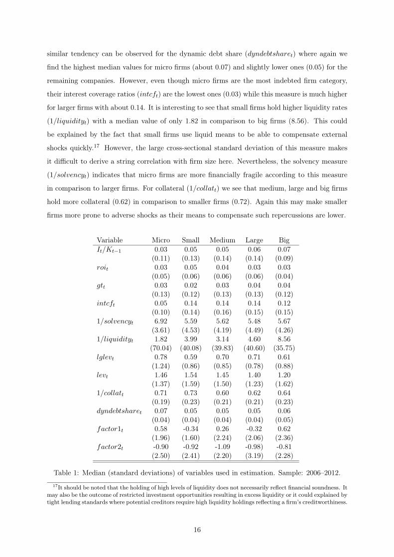
similar tendency can be observed for the dynamic debt share (dyndebtsharet) where again we

find the highest median values for micro firms (about 0.07) and slightly lower ones (0.05) for the

remaining companies. However, even though micro firms are the most indebted firm category,

their interest coverage ratios (intcft) are the lowest ones (0.03) while this measure is much higher

for larger firms with about 0.14. It is interesting to see that small firms hold higher liquidity rates

(1/liquidityt) with a median value of only 1.82 in comparison to big firms (8.56). This could

be explained by the fact that small firms use liquid means to be able to compensate external

shocks quickly.17 However, the large cross-sectional standard deviation of this measure makes

it difficult to derive a string correlation with firm size here. Nevertheless, the solvency measure

(1/solvencyt) indicates that micro firms are more financially fragile according to this measure

in comparison to larger firms. For collateral (1/collatt) we see that medium, large and big firms

hold more collateral (0.62) in comparison to smaller firms (0.72). Again this may make smaller

firms more prone to adverse shocks as their means to compensate such repercussions are lower.

Variable Micro Small Medium Large Big

It/Kt−1 0.03 0.05 0.05 0.06 0.07(0.11) (0.13) (0.14) (0.14) (0.09)

roit 0.03 0.05 0.04 0.03 0.03(0.05) (0.06) (0.06) (0.06) (0.04)

gtt 0.03 0.02 0.03 0.04 0.04(0.13) (0.12) (0.13) (0.13) (0.12)

intcft 0.05 0.14 0.14 0.14 0.12(0.10) (0.14) (0.16) (0.15) (0.15)

1/solvencyt 6.92 5.59 5.62 5.48 5.67(3.61) (4.53) (4.19) (4.49) (4.26)

1/liquidityt 1.82 3.99 3.14 4.60 8.56(70.04) (40.08) (39.83) (40.60) (35.75)

lglevt 0.78 0.59 0.70 0.71 0.61(1.24) (0.86) (0.85) (0.78) (0.88)

levt 1.46 1.54 1.45 1.40 1.20(1.37) (1.59) (1.50) (1.23) (1.62)

1/collatt 0.71 0.73 0.60 0.62 0.64(0.19) (0.23) (0.21) (0.21) (0.23)

dyndebtsharet 0.07 0.05 0.05 0.05 0.06(0.04) (0.04) (0.04) (0.04) (0.05)

factor1t 0.58 -0.34 0.26 -0.32 0.62(1.96) (1.60) (2.24) (2.06) (2.36)

factor2t -0.90 -0.92 -1.09 -0.98) -0.81(2.50) (2.41) (2.20) (3.19) (2.28)

Table 1: Median (standard deviations) of variables used in estimation. Sample: 2006–2012.

17It should be noted that the holding of high levels of liquidity does not necessarily reflect financial soundness. Itmay also be the outcome of restricted investment opportunities resulting in excess liquidity or it could explained bytight lending standards where potential creditors require high liquidity holdings reflecting a firm’s creditworthiness.

16

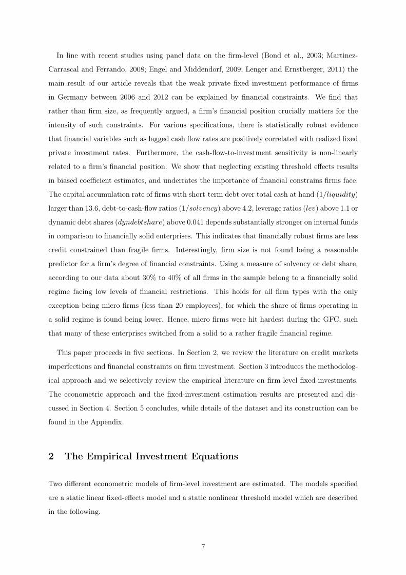
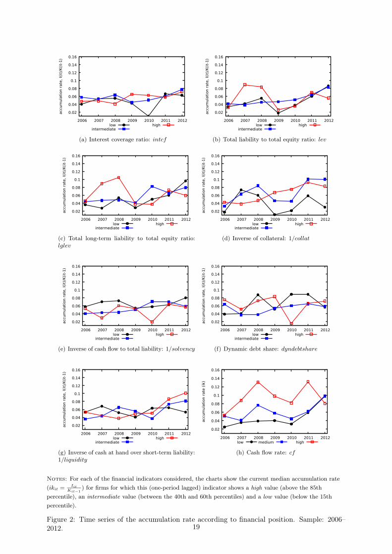
To obtain some first evidence on the relationship between a firm’s accumulation rate and its

financial position, we plot investment rates over time according to different levels of creditworthi-

ness. More concrete, we compare the investment rates of firms for which the respective pre-period

financial indicator is below the 15th percentiles (denoted by low), with firms for which the finan-

cial indicator is between the 40th and 60th percentile (intermediate) and firms with values above

the 85th percentile (high).18 Figure 2 depicts the accumulation rate for each of the balance sheet

items considered in this paper, with the only exception of the two common factors. Note, that

this is a simple unconditional correlation exercise and has to be interpreted with caution.

As can be seen in Figure 2(a), the accumulation rate is weakly correlated with firms’ interest-

coverage ratio. There is a temporary downturn of the accumulation rate for firms operating at

the lower quantiles in 2010 followed by a quick recovered. Debt has a dual character : On the

one hand more credit (for given equity), and hence higher leverage, allows firms to invest at

higher speed but this debt is also associated with high cash outflows for interest and principal

payments which may signal low creditworthiness. Also a firm might have a low leverage either

due to high equity or as its access to external credit is restricted. The dual character of debt is

partly reflected in the data. The accumulation rate of highly-leveraged firms (see Figure 2(b))

strongly exceeds the ones of the other firms in the pre-crisis period until 2008. However, the GFC

let to a more severe downturn in the accumulation rate of highly leveraged firms in comparison

to the remaining companies in the following two years. This may support the perspective that

lenders applied more strict lending standards making it harder for firms with a debt-overhang

to obtain credit at all or at least at reasonable conditions. The investment ratio of low- and

medium-leveraged firms is found being much smoother during the crisis-episode. For both low

and medium leveraged firms no adverse repercussions on investment rates can be observed; their

rates are actually increasing.

In Figure 2(f) the investment dynamics for firms grouped according to the dynamic debt share

are depicted. Firms with low levels of dynamic debt share experienced the highest accumulation

rates over the entire period on average. For firms with medium levels one can observe a smooth

investment path instead but the associated rate is slightly lower over time. Firms with a high

dynamic debt share had on average the highest investment rates until 2009 before their investment

activities massively declined. Hence, the data suggest an inverse but weak relationship between

the level of dynamic debt and a firm’s accumulation rate. Grouping firms according to their

collateral rates, 1/collat, shows that the firms with the lowers collateral also exhibit the least

18For a more detailed country-wise analysis of the impact of the recent GFC on fixed-investment see ECB (2013,p. 60ff.).

17

investment rates over time (see Figure 2(d)). This is at least visible since 2009 even though these

firms had similar investment rates as the more financially solid counterparts. Again, this suggest

that since the GFC potential lenders have tightened their lending standards which affected firms

with low collateral holdings adversely. Using solvency as a sample-splitting variable indicates

no differences in the accumulation rate of firms with intermediate and high solvency rates, as

depicted in Figure 2(e). Their investment paths are very smooth and the GFC had no adverse

repercussions. The investment dynamics of the least solvent firms are in contrast much more

volatile over time, and one can observe a temporary decline in the investment rate in 2010 here. A

firm’s liquidity position does not seem to be correlated with their accumulation rate as displayed

in Figure 2(g). This may be explained by different reasons high liquidity holdings may imply,

as argued before. Lastly, one can see a clear hierarchy between a firm’s cash flow rate and its

investments, as displayed in Figure 2(h). There is a strong positive correlation between the cash

flow rate and investment rate.

Overall, this simple graphical description provides some initial evidence for an existing link

between a firm’s financial position and its investment rates. However, the link cannot be observed

for all financial indicators. Furthermore, there maybe non-linear relationships between financial

pressure and fixed-investment growth which is in line with recent findings on the Euro area

firm-level (ECB, 2013, p. 59). This may be explained by the dual character of debt, enhancing

potential growth on the one hand but also leading to higher debt burdens accompanied by higher

real debt servicing costs on the other hand. This nonlinear relationship is partly reflected in our

estimation results as will be shown in the following.

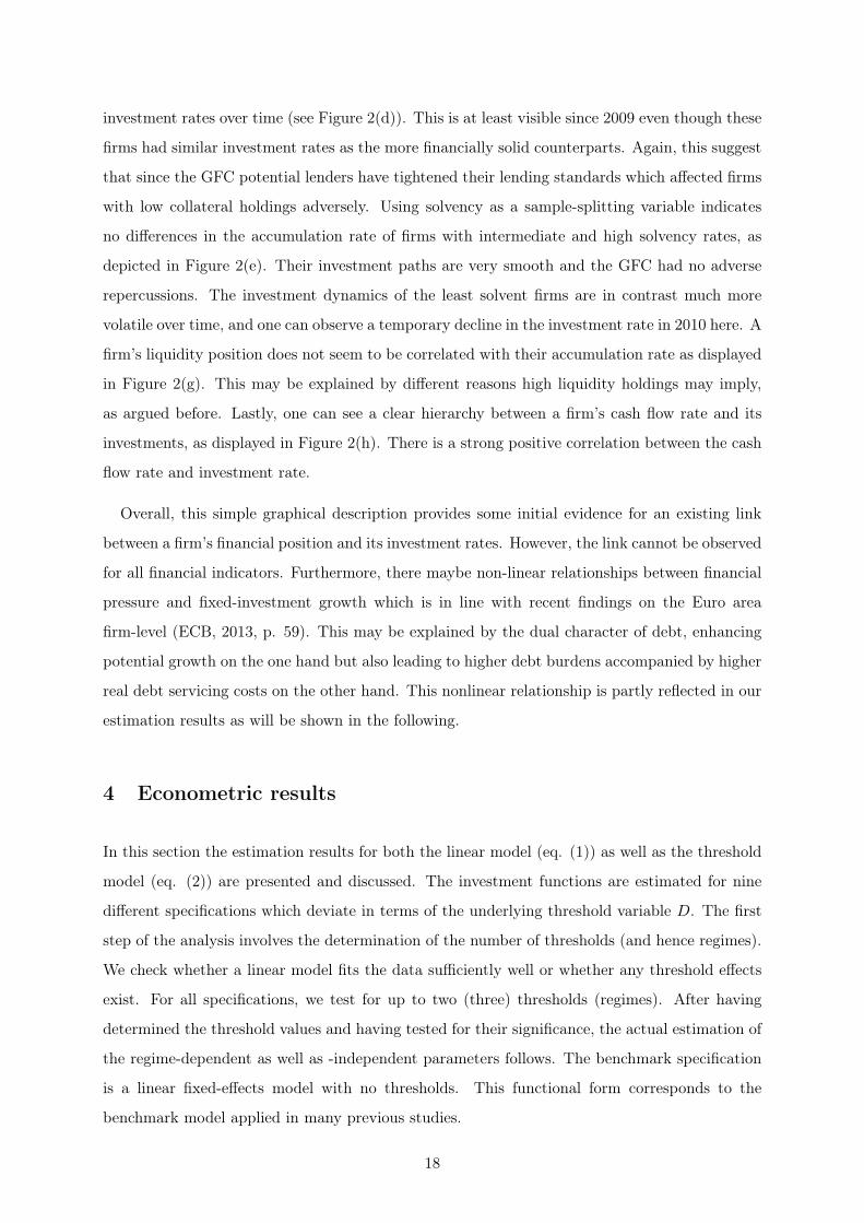
4 Econometric results

In this section the estimation results for both the linear model (eq. (1)) as well as the threshold

model (eq. (2)) are presented and discussed. The investment functions are estimated for nine

different specifications which deviate in terms of the underlying threshold variable D. The first

step of the analysis involves the determination of the number of thresholds (and hence regimes).

We check whether a linear model fits the data sufficiently well or whether any threshold effects

exist. For all specifications, we test for up to two (three) thresholds (regimes). After having

determined the threshold values and having tested for their significance, the actual estimation of

the regime-dependent as well as -independent parameters follows. The benchmark specification

is a linear fixed-effects model with no thresholds. This functional form corresponds to the

benchmark model applied in many previous studies.

18

0.02

0.04

0.06

0.08

0.1

0.12

0.14

0.16

2006 2007 2008 2009 2010 2011 2012

accum

ula

tion r

ate

, I(

it)/

K(i

t-1)

lowintermediate

high

(a) Interest coverage ratio: intcf

0.02

0.04

0.06

0.08

0.1

0.12

0.14

0.16

2006 2007 2008 2009 2010 2011 2012

accum

ula

tion r

ate

, I(

it)/

K(i

t-1)

lowintermediate

high

(b) Total liability to total equity ratio: lev

0.02

0.04

0.06

0.08

0.1

0.12

0.14

0.16

2006 2007 2008 2009 2010 2011 2012

accum

ula

tion r

ate

, I(

it)/

K(i

t-1)

lowintermediate

high

(c) Total long-term liability to total equity ratio:lglev

0.02

0.04

0.06

0.08

0.1

0.12

0.14

0.16

2006 2007 2008 2009 2010 2011 2012

accum

ula

tion r

ate

, I(

it)/

K(i

t-1)

lowintermediate

high

(d) Inverse of collateral: 1/collat

0.02

0.04

0.06

0.08

0.1

0.12

0.14

0.16

2006 2007 2008 2009 2010 2011 2012

accum

ula

tion r

ate

, I(

it)/

K(i

t-1)

lowintermediate

high

(e) Inverse of cash flow to total liability: 1/solvency

0.02

0.04

0.06

0.08

0.1

0.12

0.14

0.16

2006 2007 2008 2009 2010 2011 2012

accum

ula

tion r

ate

, I(

it)/

K(i

t-1)

lowintermediate

high

(f) Dynamic debt share: dyndebtshare

0.02

0.04

0.06

0.08

0.1

0.12

0.14

0.16

2006 2007 2008 2009 2010 2011 2012

accum

ula

tion r

ate

, I(

it)/

K(i

t-1)

lowintermediate

high

(g) Inverse of cash at hand over short-term liability:1/liquidity

0.02

0.04

0.06

0.08

0.1

0.12

0.14

0.16

2006 2007 2008 2009 2010 2011 2012

accum

ula

tion r

ate

(ik

)

low medium high

(h) Cash flow rate: cf

Notes: For each of the financial indicators considered, the charts show the current median accumulation rate

(ikit =Iit

Kit−1

) for firms for which this (one-period lagged) indicator shows a high value (above the 85th

percentile), an intermediate value (between the 40th and 60th percentiles) and a low value (below the 15th

percentile).

Figure 2: Time series of the accumulation rate according to financial position. Sample: 2006–2012. 19

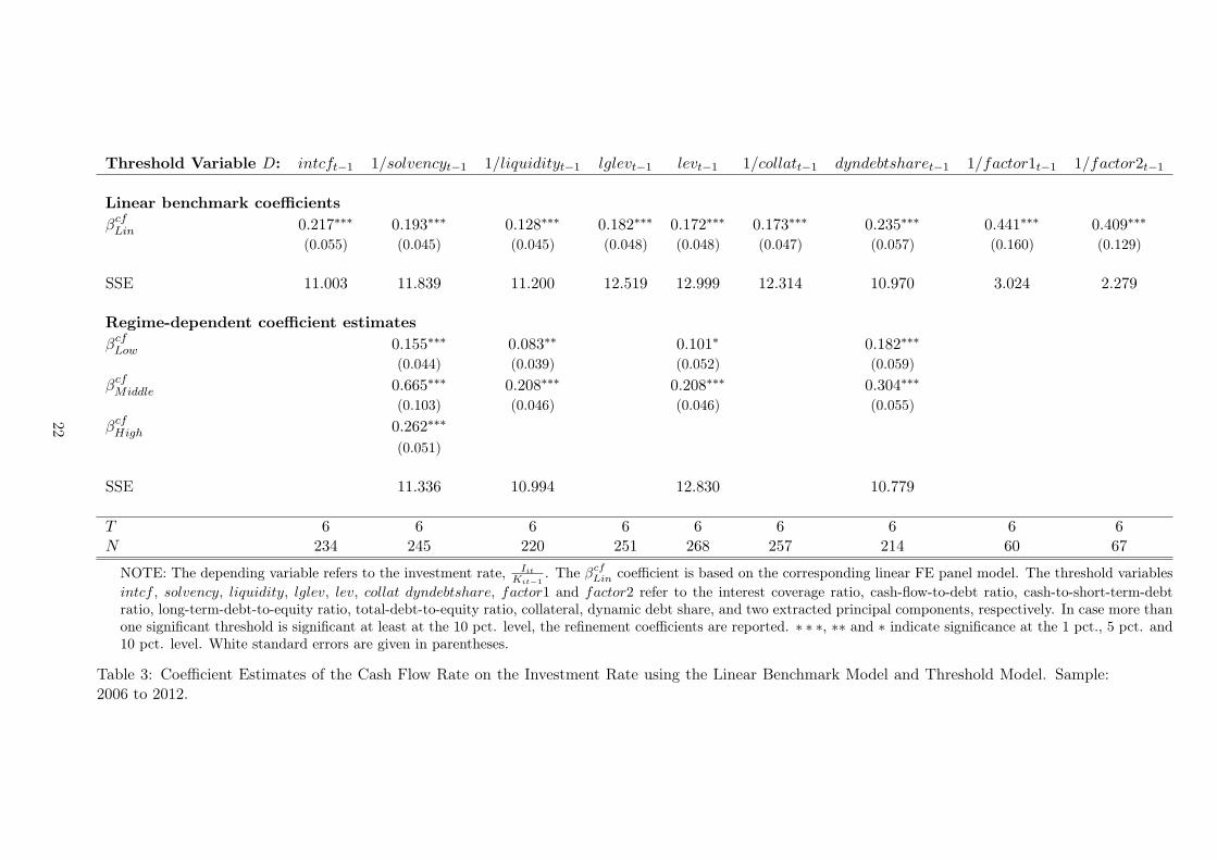
4.1 Estimation results and cash flow sensitivity of investments

First the linear model results are reported. In the first part of Table 3 the cash flow sensitivities

of investment using the linear benchmark model are reported for all nine specifications. The

respective linear coefficient estimate is denoted by βcfLin. Irrespective of the considered balance

sheet variable Dit−1, we find for all nine linear specifications positive and significant (at the 1%

level) point estimates ranging from 0.128 to 0.441. This directs attention to existing financial

constraints firms in Germany face, even though we haven’t split the sample into some categories

at this stage. Nevertheless, these results confirm previous findings as described before. However,

it should be noted that the estimates are biased and inefficient in case the true data generating

process is nonlinear.

Next, we test for nonlinear threshold effects for which the results are reported in Table 2. The

first column displays the name of the respective threshold variable Dit−1 applied as outlined in

eq. (2). The testing sequence starts with the null hypothesis of no threshold against a single

threshold (H0 : T = 0 vs. H1 : T = 1). If the null is rejected, one proceeds by testing the

null of a single threshold against two thresholds (H0 : T = 1 vs. H1 : T = 2). The second

column computes the respective bootstrap p-value, and the last two columns tabulate the point

estimates (plus 95% confidence intervals) of the threshold value(s), γ. In case more than one

threshold is found, the refinement values of γ are provided.

For four specifications evidence of regime-dependency is found. The specifications for which

thresholds effects are found separately include leverage (levit−1), the inverse solvency measure

(1/solvencyit−1), the inverse liquidity measure (1/liquidityit−1) and the dynamic debt share

(dyndebtshareit−1). Using 1/solvencyit−1 as a threshold variable, we find evidence for two

thresholds (each significant at the 1% level) and a single threshold for the levit−1 (significant at

the 5% level), dyndebtshareit−1 (significant at the 1% level) and 1/liquidityit−1 (significant at

the 5% level), respectively. Hence, at least for these four specifications a linear model results in

biased estimates of cash flow on investment.

20

Threshold Variable D : p-value γ1 γ2

Interest coverage ratio: intcfit−1

H0 : T = 0 vs. H1 : T = 1 0.229 0.064(-0.005|0.370)

H0 : T = 1 vs. H1 : T = 2 0.219 0.064 0.252(-0.005|0.370) (0.054|0.254)

Inverse of cash flow to total liability: 1/solvencyit−1

H0 : T = 0 vs. H1 : T = 1 0.002 4.187(4.030|4.187)

H0 : T = 1 vs. H1 : T = 2 0.000 4.187 4.301(4.030|4.187) (4.301|4.314)

Inverse of cash at hand over short-term liability: 1/liquidityit−1

H0 : T = 0 vs. H1 : T = 1 0.011 13.633(11.494|17.177)

H0 : T = 1 vs. H1 : T = 2 0.289 13.633 0.627(11.494|17.177) (0.466|61.691)

Total long-term liability to total equity: lglevit−1

H0 : T = 0 vs. H1 : T = 1 0.133 0.298(0.252|1.937)

H0 : T = 1 vs. H1 : T = 2 0.163 0.298 1.824(0.252|1.937) (0.621|1.937)

Total liability to total equity: levit−1

H0 : T = 0 vs. H1 : T = 1 0.033 1.145(0.670|1.893)

H0 : T = 1 vs. H1 : T = 2 0.177 1.145 2.843(0.670|1.893) (0.670|3.246)

Inverse of collateral: 1/collatit−1

H0 : T = 0 vs. H1 : T = 1 0.199 0.358(0.349|0.402)

H0 : T = 1 vs. H1 : T = 2 0.618 0.358 0.317(0.349|0.402) (0.280|0.946)

Dynamic debt share: dyndebtshareit−1

H0 : T = 0 vs. H1 : T = 1 0.005 0.041(0.041|0.045)

H0 : T = 1 vs. H1 : T = 2 0.167 0.041 0.129(0.041|0.045) (0.014|0.131)

Inverse of 1st common factor: 1/factor1it−1

H0 : T = 0 vs. H1 : T = 1 0.481 0.436(-3.117|2.385)

H0 : T = 1 vs. H1 : T = 2 0.101 0.436 0.468(-3.117|2.385) (0.468|0.468)

Inverse of 2nd common factor: 1/factor2it−1

H0 : T = 0 vs. H1 : T = 1 0.793 0.709(-4.782|3.096)

H0 : T = 1 vs. H1 : T = 2 0.004 0.709 0.766(-4.782|3.096) (0.749|0.769)

Note: The test results for multiple thresholds are provided. T0 vs. T1 andT1 vs. T2 refer to the null hypotheses of a linear model against a singlethreshold model (2 regimes) and a single threshold against a double thresholdmodel. We provide the bootstrap p-values based on 999 replications. γ1 andγ2 denote the estimated threshold values (in square brackets the 95 pct. CIsare provided). For the test on two threshold, the refinement estimates arereported. The number of quantiles checked is 300.

Table 2: Threshold Test Results. Sample: 2006 to 2012.

21

Threshold Variable D: intcft−1 1/solvencyt−1 1/liquidityt−1 lglevt−1 levt−1 1/collatt−1 dyndebtsharet−1 1/factor1t−1 1/factor2t−1

Linear benchmark coefficients

βcfLin 0.217∗∗∗ 0.193∗∗∗ 0.128∗∗∗ 0.182∗∗∗ 0.172∗∗∗ 0.173∗∗∗ 0.235∗∗∗ 0.441∗∗∗ 0.409∗∗∗

(0.055) (0.045) (0.045) (0.048) (0.048) (0.047) (0.057) (0.160) (0.129)

SSE 11.003 11.839 11.200 12.519 12.999 12.314 10.970 3.024 2.279

Regime-dependent coefficient estimates

βcfLow 0.155∗∗∗ 0.083∗∗ 0.101∗ 0.182∗∗∗

(0.044) (0.039) (0.052) (0.059)

βcfMiddle 0.665∗∗∗ 0.208∗∗∗ 0.208∗∗∗ 0.304∗∗∗

(0.103) (0.046) (0.046) (0.055)

βcfHigh 0.262∗∗∗

(0.051)

SSE 11.336 10.994 12.830 10.779

T 6 6 6 6 6 6 6 6 6N 234 245 220 251 268 257 214 60 67

NOTE: The depending variable refers to the investment rate, IitKit−1

. The βcfLin coefficient is based on the corresponding linear FE panel model. The threshold variables

intcf , solvency, liquidity, lglev, lev, collat dyndebtshare, factor1 and factor2 refer to the interest coverage ratio, cash-flow-to-debt ratio, cash-to-short-term-debtratio, long-term-debt-to-equity ratio, total-debt-to-equity ratio, collateral, dynamic debt share, and two extracted principal components, respectively. In case more thanone significant threshold is significant at least at the 10 pct. level, the refinement coefficients are reported. ∗ ∗ ∗, ∗∗ and ∗ indicate significance at the 1 pct., 5 pct. and10 pct. level. White standard errors are given in parentheses.

Table 3: Coefficient Estimates of the Cash Flow Rate on the Investment Rate using the Linear Benchmark Model and Threshold Model. Sample:2006 to 2012.

22

We report and discuss the regime-dependent coefficient estimates only for the four specifica-

tions for which significant threshold effects were found. The regime-dependent coefficients are

denoted by βcfLow, βcf

Middle and βcfHigh, respectively, and are reported in Table 3. The abbrevia-

tions refer to the marginal effect of the cash flow rate on the fixed investment rate for firms with

low, intermediate and high values of the respective threshold variable (in case three regimes are

detected). The regimes are separated by the estimated threshold value γ, as reported before in

Table 2.

The estimated threshold values for the 1/solvency measure are close to each other, having

values of γ1 = 4.187 and γ2 = 4.301, respectively. The empirical median value of 1/solvency

is 6.9 for micro firms and about 5.6 for the remaining companies. Thus the a majority of firms

in our sample belong to the rather fragile regime according to this financial measure. The

cash flow sensitivity is lowest for firms with the highest solvency measure (1/solvency ≤ 4.187)

with a coefficient of CcfLow = 0.155 (significant at the 1% level) as reported in Table 3. This

point estimate is close to the linear benchmark coefficient βCFLin = 0.193. For the intermediate

regime (4.187 < 1/solvency ≤ 4.301) the cash flow sensitivity increases to CcfMiddle = 0.665

(significant at the 1% level) and indicates much tighter financial constraints for firms falling

into this regime. Surprisingly we find for firms operating in the regime with the lowest solvency

rates (1/solvency > 4.301) still a high cash flow coefficient CcfHigh = 0.262 (significant at the

1% level) but which is much lower compared to firms in the intermediate state. Still, the effect

is almost twice as high as for firms operating in the least restrictive financial regime. This

seemingly counterintuitive result may be explained as follows: A low level of solvency does

not necessarily go hand in hand with (expected) high default risk if existing debt is sufficiently

secured by existing collateral. Table 2 reports the median collateral holdings of firms falling

into a specific regime. The statistics indicate that the most solvent firms hold higher collateral

rates (1/collateral = 0.63) while the firms falling into the intermediate regime, characterized

by the tightest financial constraints, hold the least collateral rates (1/collateral = 0.7). The

least solvent firms are, however, characterized by higher collateral holdings (1/collateral = 0.68)

as the ones in the intermediate state which may explain why the cash flow sensitivity of these

companies is lower. Thus, the tight financial restrictions firms in the intermediate regime face,

potentially result (conditional on 1/solvency) from rather low levels of collateral available to

secure their debt commitments. Creditors consciously prefer to secure their credits by collateral,

and hence collateral comprises additional key information on financial constraints.

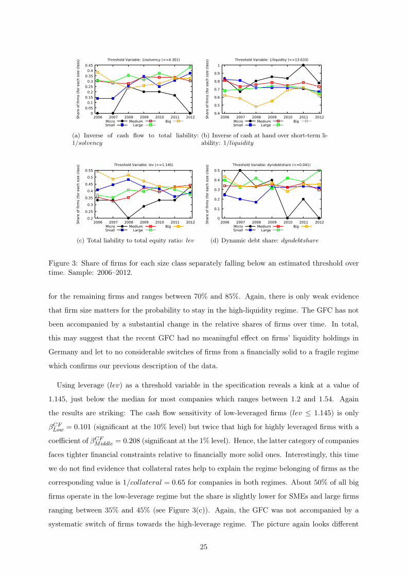
Figure 3 depicts the share of firms for each size class falling into a specific financial regime

23

over time.19 Until 2007 all micro firms operated in the low-solvency regime (1/solvency > 4.301)

(see Figure 3(a)). However, since 2008 the share of micro firms falling either into the medium-

or high-solvency regime has had increased to about 20% before decreasing again in 2012. In

contrast about 30% to 40% of all SMEs and larger firms operate at least in the intermediate

solvency-state. This result suggests that the probability to fall into a financially sound regime is

lower for micro firms in comparison to larger companies. Furthermore, small firms have caught

up in terms of solvency and stabilized their balance-sheets since 2008. Improved solvency rates

could be a consequence of increased lending standards creditors demanded after the GFC. In

total, the repercussions of the GFC on the solvency situation of firms seems to be modest, and

the correlation between the probability to stay in a specific regime and firm size is rather weak,

at least for SMEs and larger companies.

Financial regime 1/solvencyt 1/liquidityt levt dyndebtsharetLow 0.63 0.64 0.65 0.62

(0.24) (0.24) (0.25) (0.23)Middle 0.70 0.71 0.65 0.69

(0.20) (0.25) (0.25) (0.25)High 0.68

(0.24)

NOTE: The first column indicates the respective financial regime firms op-erate in, as estimated and reported in Table 2. The following three columnsreport the firms’ median value (standard deviation in brackets) of collateralholdings (1/collateral) for each specific regime.

Table 4: Median (standard deviation) collateral holdings according to the estimated regimes.Sample: 2006–2012.

Using the threshold variable 1/liquidity reveals one significant threshold at γ = 13.633. The

median value of 1/liquidity was found being 1.82 for micro firms and 8.56 for large firms im-

plying that the threshold value separates liquid from rather illiquid companies from each other.

According to the estimation results (see Table 3), the investment rate of firms with high liq-

uidity holdings (1/liquiidity ≤ 13.633) reacts less sensitive to changes in the cash flow rate

(βCFLow = 0.083 and significant at the 1% level) in comparison to firms operating in the financially

constrained regime for which βCFMiddle = 0.208 (significant at the 1% level). Again we find a corre-

lation with firms’ collateral holdings and their regime belonging: The most liquid firms facing the

least intense financial constraints are again holding higher collateral rates (1/collateral = 0.64)

compared to financially constrained companies (1/collateral = 0.71). Figure 3(b) depicts that

about 60% of all big firms operate in the high-liquidity regime. The fraction is slightly higher

19Find the corresponding plots for the remaining variables in the Appendix in Figure 4.

24

0

0.05

0.1

0.15

0.2

0.25

0.3

0.35

0.4

0.45

2006 2007 2008 2009 2010 2011 2012Share

of

firm

s (

for

each s

ize c

lass) Threshold Variable: 1/solvency (<=4.301)

MicroSmall

MediumLarge

Big

(a) Inverse of cash flow to total liability:1/solvency

0.4

0.5

0.6

0.7

0.8

0.9

1

2006 2007 2008 2009 2010 2011 2012Share

of

firm

s (

for

each s

ize c

lass) Threshold Variable: 1/liquidity (<=13.633)

MicroSmall

MediumLarge

Big

(b) Inverse of cash at hand over short-term li-ability: 1/liquidity

0.2

0.25

0.3

0.35

0.4

0.45

0.5

0.55

2006 2007 2008 2009 2010 2011 2012Share

of

firm

s (

for

each s

ize c

lass) Threshold Variable: lev (<=1.145)

MicroSmall

MediumLarge

Big

(c) Total liability to total equity ratio: lev

0

0.1

0.2

0.3

0.4

0.5

2006 2007 2008 2009 2010 2011 2012Share

of

firm

s (

for

each s

ize c

lass) Threshold Variable: dyndebtshare (<=0.041)

MicroSmall

MediumLarge

Big

(d) Dynamic debt share: dyndebtshare

Figure 3: Share of firms for each size class separately falling below an estimated threshold overtime. Sample: 2006–2012.

for the remaining firms and ranges between 70% and 85%. Again, there is only weak evidence

that firm size matters for the probability to stay in the high-liquidity regime. The GFC has not

been accompanied by a substantial change in the relative shares of firms over time. In total,

this may suggest that the recent GFC had no meaningful effect on firms’ liquidity holdings in

Germany and let to no considerable switches of firms from a financially solid to a fragile regime

which confirms our previous description of the data.

Using leverage (lev) as a threshold variable in the specification reveals a kink at a value of

1.145, just below the median for most companies which ranges between 1.2 and 1.54. Again

the results are striking: The cash flow sensitivity of low-leveraged firms (lev ≤ 1.145) is only

βCFLow = 0.101 (significant at the 10% level) but twice that high for highly leveraged firms with a

coefficient of βCFMiddle = 0.208 (significant at the 1% level). Hence, the latter category of companies

faces tighter financial constraints relative to financially more solid ones. Interestingly, this time

we do not find evidence that collateral rates help to explain the regime belonging of firms as the

corresponding value is 1/collateral = 0.65 for companies in both regimes. About 50% of all big

firms operate in the low-leverage regime but the share is slightly lower for SMEs and large firms

ranging between 35% and 45% (see Figure 3(c)). Again, the GFC was not accompanied by a

systematic switch of firms towards the high-leverage regime. The picture again looks different

25

for micro firms: In 2008 the share of micro firms in the low-leverage regime fell from 35% to 20%

before these companies were able to de-leverage again, improving their financial position.

The overall picture remains valid using the dynamic debt share as a potential threshold vari-

able. We find a single significant threshold at γ1 = 0.041 separating lowly indebted from highly

indebted companies. The median value of dyndebtshare ranges from 0.05 to 0.07. For firms

operating in the low-debt regime, we find a cash flow sensitivity of about βCFLow = 0.181 but a

much higher one for firms in the high-debt regime, βCFMiddle = 0.304 (both significant at the 1%

level). Furthermore, the least constraint firms hold higher collateral rates (1/collateral = 0.62)

as the constrained ones (1/collateral = 0.69). About 35% to 45% of all medium-sized, large and

big companies operate in the low-debt regime, as depicted by Figure 3(d). Between 2006 and

2008 only 20% of all small companies were located in the low-debt regime, but the fraction has

increased to 30% since 2009 suggesting some deleveraging process for these units. The corre-

sponding share of micro firms fluctuates between 25% and 40% between 2006 and 2009 before

the fraction has substantially declined since then. This indicates that SMEs and larger firms

were able to compensate the adverse effects of GFC much better in comparison to micro firms

which had to increase their dynamic debt shares, such that many micro firms switched out of

the low-debt regime into the high-debt regime.

Overall, we find strong evidence that firms in Germany face financial constraints. Furthermore,

the results indicate a specific regime dependency saying that the degree of financial constraint-

ness is much more intense for firms with weak balance sheets. Additionally, these financially

constrained firms are characterized by rather low levels of collateral. However, firm size, as often

argued, does not play a prominent role even though it cannot be fully neglected. The latter

aspect supports the findings of Martinez-Carrascal and Ferrando (2008) who also do not find

evidence that firm size matters for the degree of financial restrictions firms face. According to

our estimation, an exception may be micro firms for which we find, in comparison to larger

companies. In comparison, a higher fraction of micro firms holds rather high levels of liquidity

(probably reflecting tight lending standards applied), are more frequently belonging to the high-

leverage regime and are rather characterized by low levels of solvency. Nonetheless, the results

should be seen with caution as the number of micro firms in our sample is relatively low with

only about 10 cross-sectional units.

Regime-independent coefficient estimates Lastly, we briefly present the estimation results

of the regime-independent coefficients which are provided in Table 5. For most specifications we

find a negative effect of the number of workers (in logs) on capital accumulation. Growth of real

26

sales revenue is not statistically significant in any of the models. Real return on investment seems

to be positively but concavely related to capital accumulation. The effect of the depreciation

rate, d, is always positive, but there is also evidence for a concave relationship between d and

the investment rate. This is in line with the findings of the Bundesbank showing that deduction

is a major source of internal funding for firms (Bundesbank, 2012). The great financial crisis

is accompanied by a significant positive level shift in the investment rate. Additionally, the

interaction term gfc ∗ w indicates that the effect of the GFC on capital accumulation increases

in firm size measured by the (log) number of workers. Hence, larger firms were better able to

cope with the repercussions of the economic crisis in comparison to smaller firms. Furthermore,

firm-level investment is contemporaneously and pro-cyclically related to the output gap, gdp.

However, most interestingly there is only weak evidence for a relationship between capital

accumulation and the lagged level of the respective threshold variable. Only for the interest

coverage ratio (intcf), the dynamic debt share (dyndebtshare) and the second common factor

(factor2) a significant (at least at the 10% level) effect is found. The level of the interest coverage

ratio is negatively related to the investment rate while the two other effects are positive. This

mirrors the dual character of debt, as argued before. Overall, this result highlights an additional

channel through which financial conditions may affect realized investments: The status of the

balance-sheet not only has indirect effects on investments by providing signals of creditworthiness

but may also affect the accumulation rate by e.g. restricting the amount of available internal

funds. However, to be a valid finding this potential channel needs to be analyzed in more detail

in future research.

27

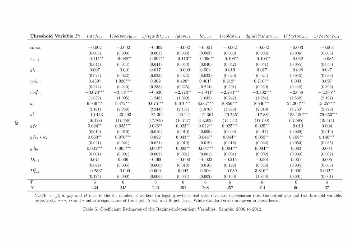
Threshold Variable D: intcft−1 1/solvencyt−1 1/liquidityt−1 lglevt−1 levt−1 1/collatt−1 dyndebtsharet−1 1/factor1t−1 1/factor2t−1

const −0.002 −0.002 −0.002 −0.002 −0.001 −0.002 −0.002 −0.003 −0.003(0.003) (0.003) (0.003) (0.003) (0.003) (0.003) (0.003) (0.006) (0.005)

wt−1 −0.111∗∗ −0.088∗∗ −0.094∗∗ −0.113∗∗ −0.096∗∗ −0.108∗∗ −0.104∗∗ −0.062 −0.085(0.044) (0.044) (0.044) (0.043) (0.040) (0.042) (0.051) (0.055) (0.056)

gtt−1 0.007 −0.001 0.017 −0.009 0.002 0.019 0.017 −0.026 0.027(0.024) (0.023) (0.023) (0.023) (0.022) (0.020) (0.024) (0.043) (0.034)

roit−1 0.439∗ 1.026∗∗∗ 0.362 0.426∗ 0.401∗ 0.512∗∗ 0.710∗∗∗ 0.033 0.097(0.244) (0.240) (0.238) (0.225) (0.214) (0.201) (0.260) (0.442) (0.392)

roi2t−1 −3.020∗∗∗ −3.447∗∗∗ −0.636 −2.770∗∗ −1.941∗ −2.764∗∗∗ −3.402∗∗∗ −2.658 −4.385∗∗

(1.039) (1.095) (1.246) (1.069) (1.032) (0.947) (1.284) (2.562) (2.197)

dt 6.946∗∗∗ 9.472∗∗∗ 9.075∗∗∗ 9.670∗∗∗ 8.067∗∗∗ 8.856∗∗∗ 8.546∗∗∗ 24.206∗∗∗ 15.257∗∗∗

(2.181) (2.258) (2.244) (2.151) (1.876) (1.983) (2.319) (4.753) (2.829)

d2t −10.443 −23.493 −25.304 −24.241 −12.364 −26.735∗ −17.881 −153.150∗∗∗ −79.653∗∗∗

(16.428) (17.356) (17.769) (16.747) (14.509) (15.434) (17.790) (37.595) (19.574)

gfc 0.024∗∗ 0.035∗∗∗ 0.026∗∗ 0.023∗∗ 0.022∗∗ 0.025∗∗∗ 0.025∗∗ −0.013 0.004(0.010) (0.010) (0.010) (0.010) (0.009) (0.009) (0.011) (0.020) (0.016)

gfct ∗ wt 0.053∗∗ 0.076∗∗∗ 0.022 0.043∗∗ 0.044∗∗ 0.044∗∗ 0.052∗∗ 0.108∗∗ 0.140∗∗∗

(0.021) (0.021) (0.021) (0.019) (0.019) (0.018) (0.022) (0.050) (0.035)

gdpt 0.005∗∗∗ 0.005∗∗∗ 0.003∗∗ 0.003∗∗ 0.004∗∗∗ 0.004∗∗∗ 0.004∗∗ 0.003 0.004(0.001) (0.001) (0.002) (0.001) (0.001) (0.001) (0.002) (0.003) (0.002)

Dt−1 0.071 0.006 −0.000 −0.006 −0.023 −0.215 −0.501 0.001 0.005(0.084) (0.005) (0.000) (0.018) (0.016) (0.198) (0.353) (0.004) (0.005)

D2t−1 −0.233∗ −0.000 0.000 0.002 0.000 −0.039 3.816∗∗ 0.000 0.002∗∗

(0.125) (0.000) (0.000) (0.004) (0.002) (0.160) (1.839) (0.001) (0.001)

T 6 6 6 6 6 6 6 6 6N 234 245 220 251 268 257 214 60 67

NOTE: w, gt, d, gdp and D refer to the the number of workers (in logs), growth of real sales revenues, depreciation rate, the output gap and the threshold variable,respectively. ∗ ∗ ∗, ∗∗ and ∗ indicate significance at the 1 pct., 5 pct. and 10 pct. level. White standard errors are given in parentheses.

Table 5: Coefficient Estimates of the Regime-independent Variables. Sample: 2006 to 2012.

28

4.2 A word of caution

A critical point in estimating reduced-form fixed-investment functions concerns the issue of con-

trolling for demand effects. One issue refers to the question whether Tobin’s q or growth in sale

revenues fully capture demand effects. If this identification issue remains unsolved, it is unclear

whether the positive cash flow effect stems from a shift on the demand side or whether it has

its causes in increased capital market imperfections emerging from the supply side. Hence, for

identification one needs to make sure that the control variables fully capture shifts in demand in

order to interpret the marginal effect of cash flow as reflecting supply side factors.

In their, unfortunately, less known paper Fazzari and Petersen (1993) have suggested an ex-

tension of their initially proposed estimation approach. The authors emphasize the dual role of

working capital as a use of funds as well as a source of liquidity.20 The authors start their argu-

ment by computing the correlation between working capital and fixed-investment. As working

capital behaves pro-cyclically and is positively correlated with sales and profits, the inclusion

of working capital into the fixed-investment function should result in a positive effect on fixed-

investment. However, this only holds true if working capital as a use of funds does not compete

with fixed-investment under a binding financial constraint. Thus, for firms facing imperfect

capital markets, the marginal effect of working capital is expected to be negative.

Secondly, Fazzari and Petersen claim that the standard reduced-form fixed-investment model

underestimates the full effect of capital market imperfections. They argue that the coefficients

estimated only reflect an "...average ’short-run’ impact of cash flow shocks, after the firm engages

in optimal investment smoothing" (Fazzari and Petersen, 1993, p. 329). In order to fully capture

financing constraints one has to control for endogenous changes in working capital as a source

of fund mitigating cash flow shocks. If one does not control for working capital in the fixed-

investment function, one cannot rule out that e.g. negative cash flow shocks are compensated

by the liquidity working-capital provides (especially cash holdings). If a firm holds a large stock

of working capital, the negative cash flow shock may be compensated. However, the same shock

will have a much larger impact on investment if the stock of working capital is small and does not

allow to smooth investment plans. Under this argumentation, the previously reported results,

due to the non-consideration of working capital in our investment function, may only capture the

very short-run cash-flow-to-fixed-investment sensitivity but not the long-run effects. In Fazzari

and Petersen’s study the marginal effect of cash flow on fixed-investment is found being indeed

20Working capital is defined as the difference between short-term assets comprising accounts receivable, inven-tories and cash, minus the sum of accounts payable plus short-term debt.

29

three to four times higher after considering working-capital as an additional regressor.

Unfortunately, the DAFNE dataset includes a high number of missing observations for working

capital. However, we estimated linear benchmark models including the contemporaneous effect of

working capital as an additional regressor. Overall its point estimate was found being significant

and positive. Surprisingly, the effect on the cash flow sensitivity was rather negligible. These

results are not reported here as the number of observations is too small to be sufficiently reliable.

This short paragraph is added to outline remaining limitation of our own work and of others on

measuring financial investment constraints.

Another aspect concerns the substitution effect. The financing instruments a firm can choose,

include among others equity, bank loans, debt securities, inter-company loans, trade credit fa-

cilities or informal loans. Thus, firms are to some degree flexible in their financing strategies.

However, it should be kept in mind that this flexibility is rather limited for typically informa-

tionally opaque SMEs. On the aggregate level there is evidence that in some Euro area countries

corporations have replaced bank loans with market-based funding instruments such as equity

and debt securities, trade credit as well as intra-sectoral financing between firms (ECB, 2013, p.

21ff.).21 A strong substitution channel may mitigate the relevance of financial frictions stemming

from bank credits. However, to control for substitution effects is demanding as an appropriate

model requires a multivariate or instrumental variable set-up in order to control for endogeneity

issues.

Lastly one should mention the potential repercussions of the recent financial crisis on the

estimation results. It might be the case that the relationships between the variables have changed

as a result of deeper structural changes due to the GFC. In this article we have dealt with this

issue by including a simple shift dummy which accounts for possible changes in the conditional

mean of the accumulation rate, as well as an interaction term between the shift dummy and the

(log) number of workers. The latter regressor controls for differences in the repercussions of the

GFC depending on firm size. This may be justified for two reasons: First, the article is about

the relationship between realized firm investment, cash flow and balance sheet aspects. Thus,

the GFC, captured in the data, may even provide information on rare events which helps us to

identify specific regimes. Second, as the time span covered is rather small, it is difficult to detect

parameter changes due to breaks over time using the econometric model applied. Nevertheless,

the question of how the GFC might have impacted on the relationships between investment, cash

flow and balance sheet measures is definitely of importance but should be addressed in another

21See also Casey and O’Toole (2013) for empirical evidence on the use of alternative sources of finance byEuropean SMEs during the financial crisis.

30

paper using a longer time span.

5 Policy Implications and Summary

This article has shown that a firm’s financial situation matters. In particular, it has linked firms’

balance-sheet positions to fixed capital accumulation. The paper contributes to the literature

on financial investment constraints which has gained renewed interest during the recent financial

crisis (IMF, 2015). The results from the estimation of investment functions reveal a significant

and positive effect of cash flow on fixed-investment. This confirms major previous findings in

the literature. Additionally, there is evidence that the cash-flow-investment nexus is regime-

dependent as the marginal effect of cash flow on capital accumulation is lower for financially

solid firms in comparison to fragile ones. The differences in the magnitude are substantial for

some specifications. Neglecting those nonlinearities results in biased coefficient estimates and

underrates the relevance of financial constraints firms face.

In contrast to standard contentions, we find only limited evidence that firm size is a relevant

variable to discriminate between financially constrained and unconstrained companies. It is

argued that balance sheet indicators are more appropriate to separate firms accordingly. The

only exception are micro firms for which the probability to fall into a financial constrained regime

is found being higher in comparison to other size classes. During the recent financial crisis period,

a considerable share of micro firms switched from a solid financial state to a fragile one. This

suggests that micro firms were hit hardest by the recent downturn. Our results clearly stress

that a symmetric macro-wide shock such as the recent financial crisis may have asymmetric

repercussions across heterogeneous firms.

Our findings help to explain the persistence of low investment growth in Germany over the

past decade. There is direct evidence that stresses the role of financial frictions in restricting

the availability of credit to firms (Hall, 2011; Stock and Watson, 2012). This channel may also

explain the long-lasting weak labor market development in Germany at the beginning of the

2000s, as restricted access to credit may result in persistent insufficient aggregate demand and

forces firms to purge excess labor. Chodorow-Reich (2013) has recently studied the link between

the health of a firm’s lenders and a firm’s employment outcomes, and finds an economically

important relationship.

As statistical numbers indicate, German firms were on average less indebted (according to

standard balance-sheet measures) compared to firms e.g. in Italy, Spain, Greece or Portugal

31

before the GFC. Thus, the share of firms falling into the financially fragile regime is rather

low in Germany. However, this may be different for economies in the periphery, and helps to

explain why the "deleveraging-aggregate demand" channel recently emphasized by Mian and

Sufi (2010) is less prevalent in Germany in comparison to other crisis countries. As firms and

households face high debt burdens and restricted access to external finance, they are forced to

de-leverage which has severe negative repercussions on aggregate demand (Biggs et al., 2010;

Keen, 2010; Eggertsson and Krugman, 2012; Mian et al., 2013). These links also help to point

out why the downturn accelerated in 2008 much stronger in these southern European economies

in comparison to Germany. Furthermore, it also provides an explanation of why the negative

economic repercussions of the GFC were rather limited in Germany in the period after 2008.

Finally, the finding that the financial regime a firm operates in does not depend on firm size

may highlight the working of relationship-banking in Germany. The literature suggests that

relationship-banking still plays a prominent role in Germany (Memmel et al., 2008). SMEs

typically hold long-term relationships with a single or a small number of banks which are mostly

public non-profit maximizing institutions. Relationship-lending can be a meaningful institutional

device to mitigate the impact of unforeseen events and/or asymmetric information problems on

credit lending (Gobbi and Sette, 2012). A bank-based system with widespread relationship-

banking characteristics may explain, why for German SMEs the degree of financial constraintness

in terms of access to external funds is rather low over the business cycle. Unfortunately, data

constraints limit further investigation on this issue but future research should put a focus on

whether relationship-banking aspects help to resolve the weak correlation between firm size and

the degree of financial frictions in Germany.

The implications for economic policy can be briefly summarized as follows: Stimulating ag-

gregate demand may foster firm-level investments, but is most likely not sufficient. According

to the results, corporate indebtedness impedes investment, and thus economic policy must find

instruments to deal with excessive debt and non-performing loans. Furthermore, policies should

be aimed at improving the access to capital at lower costs.

32

Data Appendix

The list of industrial sectors considered is provided in Table 6 below.

Industrial sectors included

Mining and quarryingManufacturingElectricity, gas, steam and air conditioning supplyWater supply, sewerage, waste management and remediation actConstructionWholesale and retail trade; repair; repair of motor vehicles and motorcyclesTransportation and storageAccommodation and food service activitiesInformation and communication

Table 6: Overview of industries considered in the dataset

Variable definition and sources All data are taken from the Creditreform DAFNE database,

as long as not differently stated.

Investment to capital stock ratio, iki,t =∆Ki,t

Ki,t−1

=Ii,t

Ki,t−1

, is the ratio of the change in tangible

fixed assets over tangible fixed assets of the previous period. Tangible fixed assets consists of

land, property, plant and equipment.

Cash flow over tangible fixed assets, cfi,t =Cfi,tK,t−1

, is the ratio of profits after taxes and interest

over tangible fixed assets of the previous period.

Depreciation on fixed assets over tangible fixed assets, di,t =DPi,t

K,t−1. The depreciation on fixed

assets had to be imputed due to missing values for all units calculating it alternatively by:

depreciation on total assets weighted by the ratio of tangible fixed assets to total assets. This

approach closely follows Engel and Middendorf (2009).

Real return on investment roii,t is the nominal return on investment minus GDP price level

inflation rate (AMECO: PVGD).

Growth of real sales revenue, gti,t, where nominal sales revenue is deflated by GDP price level

(AMECO: PVGD).

Log of the number of workers per firm, wi,t.

Total liabilities to total equity ratio, levi,t.

Total liabilities minus short-term liabilities (maturity up to one year) to total equity ratio, lglevi,t.

Interest coverage ratio, intcfi,t, equals interest expenditures minus interest income to cash flow

ratio, intcfi,t =Inti,tCf,t

33

Solvency measures the cash flow to total liability ratio, solvencyi,t.

Collateral equals the sum of total inventory stock, tangible assets plus cash available at hand or

at bank, over total tangible assets, collati,t.

Liquidity is the ratio of cash at hand over short-term debt, liquidityi,t.

Real GDP output gap, gdpt, (AMECO: AVGDGP).

Great Financial Crisis, gfct, is dummy variable which takes unity for observations T ≥ 2008,

otherwise zero.

Screening procedure The following screening procedure has been applied to the data to avoid

excessive outliers or further implausible values.

• Drop observations with negative values for the following variables: w, lev, lglev, liquidity,

collat and dyndebtshare.

• Drop observations for which w ≤ 0.

• Drop observations of the 5% and 95% percentiles of the following variable: ik, intcf ,

solvency, liquidity, lglev, lev, collat, dyndebtshare, factor1 and factor2.

• Drop observations of the 97.5% percentiles of the following variable: w, roi.

• Drop observations of the 95% percentiles of the following variable: cf , d.

• Drop observations of the 2.5% and 97.5% percentiles of the following variable: gt.

34

References

Andrews, D. W. K. and W. Ploberger (1994). Optimal tests when a nuisance parameter is present

only under the alternative. Econometrica 62 (6), pp. 1383–1414.

Audretsch, D. B. and J. A. Elston (2002). Does firm size matter? Evidence on the impact

of liquidity constraints on firm investment behavior in Germany. International Journal of

Industrial Organization 20 (1), 1–17.

Barnett, S. A. and P. Sakellaris (1998). Nonlinear response of firm investment to q: Testing a

model of convex and non-convex adjustment costs. Journal of Monetary Economics 42 (2),

261–288.

Berger, A. and G. Udell (2006). A more complete conceptual framework for sme finance. Journal

Of Banking And Finance (30), 2945–2966.

Berger, A. N. and G. F. Udell (1998). The economics of small business finance: The roles of

private equity and debt markets in the financial growth cycle. Journal of Banking & Fi-

nance 22 (6-8), 613–673.

Bernanke, B. S. and M. Gertler (1989). Agency costs, net worth, and business fluctuations.

American Economic Review 79 (1), 14–31.

Biggs, M., T. Mayer, and A. Pick (2010). Credit and economic recovery: Demystifying phoenix

miracles. SSRN eLibrary .

Bond, S., J. A. Elston, J. Mairesse, and B. Mulkay (2003). Financial factors and investment in

belgium, france, germany, and the united kingdom: A comparison using company panel data.

The Review of Economics and Statistics 85 (1), 153–165.

Bond, S. and C. Meghir (1994). Dynamic investment models and the firm’s financial policy.

Review of Economic Studies 61, 197–222.

Boot, A. W. (2000). Relationship banking: What do we know? Journal of Financial Interme-

diation 9 (1), 7 – 25.

Bordo, M. D. and J. G. Haubrich (2010). Credit crises, money and contractions: An historical

view. pp. 1–18.

Bundesbank, D. (2012, January). Long-term developments in corporate financing in germany –

evidence based on the financial accounts. Monatsberichtsaufsatz, Deutsche Bundesbank.

Casey, E. and C. O’Toole (2013). Bank-lending constraints and alternative financing during the

financial crisis: Evidence from European SMEs. Papers WP450, Economic and Social Research

Institute (ESRI).

Chan, K. S. (1993). Consistency and limiting distribution of the least squares estimator of a

threshold autoregressive model. The Annals of Statistics 21 (1), 520–533.

35

Chirinko, R. S. and U. von Kalckreuth (2002). Further evoidence on the realtionship between

firm investment and financial status. Technical report, Deutsche Bundesbank.

Chodorow-Reich, G. (2013). The employment effects of credit market disruptions: Firm-level

evidence from the 2008-9 financial crisis. The Quarterly Journal of Economics 129 (1), 1–59.

Cottrell, A. and R. Lucchetti (2013). Gretl User’s Guide.

Cummins, J. G., K. A. Hassett, and S. D. Oliner (2006). Investment behavior, observable

expectations, and internal funds. American Economic Review 96 (3), 796–810.

Duchin, R., O. Ozbas, and B. A. Sensoy (2010). Costly external finance, corporate investment,

and the subprime mortgage credit crisis. Journal of Financial Economics 97 (3), 418–435.

Duessenberry, J. S. (1958). Business cycles and economic growth. New York: McGraw-Hill.

ECB (2013, Aug.). Corporate finance and economic activity in the euro area. Occational Paper

Series 151, European Central Bank.

ECB (2014, July). Monthly bulletin. Monthly bulletin, European Central Bank.

Eggertsson, G. B. and P. Krugman (2012). Debt, Deleveraging, and the Liquidity Trap: A

Fisher-Minsky-Koo Approach. The Quarterly Journal of Economics 127 (3), 1469–1513.

Engel, D. and T. Middendorf (2009, November). Investment, internal funds and public banking

in Germany. Journal of Banking & Finance 33 (11), 2132–2139.

Fazzari, S. M. and M. J. Athey (1987). Asymmetric information, financing constraints, and

investment. The Review of Economics and Statistics 69 (3), pp. 481–487.

Fazzari, S. M., R. G. Hubbard, and B. C. Petersen (1988). Financing constraints and corporate

investment. Brookings Papers on Economic Activity 1988 (1), 141–206.

Fazzari, S. M. and B. C. Petersen (1993). Working capital and fixed investment: New evidence

on financing constraints. RAND Journal of Economics 24 (3), 328–342.

Fischer, T. R. (1986). Entscheidungskriterien für Gläubiger. Neue betriebswirtschaftliche

Forschung. Wiesbaden: Gabler.

Fok, D., D. van Dijk, and P. H. Franses (2005). A multi-level panel star model for us manufac-

turing sectors. Journal of Applied Econometrics 20 (6), 811–827.

Fuss, C. and P. Vermeulen (2006). The response of firms‘ investment and financing to adverse

cash flow shocks: the role of bank relationships. Working Paper Series 0658, European Central

Bank.

Gaiotti, E. (2013). Credit availability and investment: Lessons from the “great recession”. Euro-

pean Economic Review 59 (C), 212–227.

Gertler, M. and S. Gilchrist (1994). Monetary policy, business cycles, and the behavior of small

manufacturing firms. The Quarterly Journal of Economics 109 (2), 309–40.

36

Gobbi, G. and E. Sette (2012). Relationship lending in a financial turmoil. Mo.Fi.R. Working

Papers 59, Money and Finance Research group (Mo.Fi.R.) - Univ. Politecnica Marche - Dept.

Economic and Social Sciences.

Gonzalez, A., T. Teräsvirta, and D. van Dick (2005). Panel smooth transition regression models.

SSE/EFI Working Paper Series in Economics and Finance 604.

Größl-Gschwendtner, I. (1993). Kreditrationierung: Mikroökonomische begründung und

makrökonomische konsequenzen. Jahrbücher für Nationalökonomie und Statistik 212 (1-2),

120–139.

Hall, R. E. (2011). The high sensitivity of economic activity to financial frictions. Economic

Journal 121 (552), 351–378.

Hansen, B. E. (1999). Threshold effects in non-dynamic panels: Estimation, testing, and infer-

ence. Journal of Econometrics 93 (2), 345–368.

Hansen, P. S. (1996, July). Permanent effects of monetary policy in a dynamic menu cost model.

Economics Letters 52 (1), 61–66.

Harhoff, D. (1998). Are there financing constraints for r&d and investment in german manufac-

turing firms. Annales d’Economie et de Statistique (49-50), 421–456.

Himmelberg, C. P. and B. C. Petersen (1994). R&d and internal finance: A panel study of small

firms in high-tech industries. The Review of Economics and Statistics 76 (1), 38–51.

Hoshi, T., A. K. Kashyap, and D. Scharfstein (1991). Corporate structure, liquidity, and invest-

ment: Evidence from japanese panel data. Quarterly Journal of Economics 106, 33–66.

Hu, X. and F. Schiantarelli (1998). Investment and capital market imperfections: A switching

regression approach using u.s. firm panel data. Review of Econometrics and Statistics 80,

466–479.

Hubbard, R. G. (1998). Capital-market imperfections and investment. Journal of Economic

Literature 36 (1), 193–225.

IMF (2015). World economic outlook. uneven growth. short- and long-term factors. Technical

report, International Monetary Fund.

Jaffee, D. M. and T. Russell (1976). Imperfect information, uncertainty, and credit rationing.

The Quarterly Journal of Economics 90 (4), pp. 651–666.

Kalecki, M. (1937). The principle of increasing risk. Economica 4, 440–447.

Keen, S. (2010). Deleveraging is america’s future. Real-world economics review (54), 32–40.

Lenger, S. and J. Ernstberger (2011). Das finanzierungsverhalten deutscher unternehmen –

hinweise auf eine kreditklemme? Kredit und Kapital 44 (3), 367–392.

37

Martinez-Carrascal, C. and A. Ferrando (2008). The impact of financial position on investment:

an analysis for non-financial corporations in the euro area. Working Paper 0820, Banco de

Espagna.

Memmel, C., C. Schmieder, and I. Stein (2008). Relationship lending - empirical evidence for

germany. Economic and Financial Reports 2008/1, European Investment Bank, Economics

Department.

Mian, A., K. Rao, and A. Sufi (2013). Household balance sheets, consumption, and the economic

slump. The Quarterly Journal of Economics 128 (4), 1687–1726.

Mian, A. R. and A. Sufi (2010). Household leverage and the recession of 2007 to 2009. NBER

Working Papers 15896, National Bureau of Economic Research, Inc.

Minsky, H. P. (1975). John Maynard Keynes. Columbia New York University Press.

Minsky, H. P. (2008). Stabilizing An Unstable Economy (1st ed.). McGraw-Hill.

Modigliani, F. and M. H. Miller (1958). The cost of capital, corporate finance and the theory of

investment. American Economic Review 48, 261–297.

Oliner, S. and G. Rudebusch (1992). Sources of financing hierarchy for business investment. The

Review of Economic and Statistics 74, 643–654.

Petersen, M. A. and R. G. Rajan (1994). The benefits of lending relationships: Evidence from

small business data. The Journal of Finance 49 (1), pp. 3–37.

Robinson, J. (1966). The Accumulation of Capital (2nd ed.). Macmillan: London.

Schiantarelli, F. (1995). Financial constraints and investment: a critical review of methodological

issues and international evidence. Conference Series ; [Proceedings] 39, 177–226.

Silva, F. and C. Carreira (2012). Measuring Firms’ Financial Constraints: A Rough Guide.

GEMF Working Papers 2012-14, GEMF - Faculdade de Economia, Universidade de Coimbra.

Stiglitz, J. and B. Greenwald (2003, October). Towards a New Paradigm in Monetary Economics.

Raffaele Mattioli Lectures. Cambridge: Cambridge University Press.

Stiglitz, J. E. (2015). Towards a general theory of deep downturns. NBER Working Papers

21444, National Bureau of Economic Research, Inc.

Stiglitz, J. E. and A. Weiss (1981). Credit rationing in markets with imperfect information. The

American Economic Review 71 (3), 393–410.

Stock, J. H. and M. W. Watson (2012). Disentangling the channels of the 2007-09 recession.

Brookings Papers on Economic Activity 44 (1 (Spring)), 81–156.

Tobin, J. (1956). Liquidity Preference as Behavior Towards Risk. Cowles Foundation Discussion

Papers 14, Cowles Foundation for Research in Economics, Yale University.

38

Townsend, R. M. (1979). Optimal contracts and competitive markets with costly state verifica-

tion. Journal of economic theory 2, 265–293.

Vetter, S. and J. Köhler (2014, March). Unternehmensdemographie und -dynamik in europa.

Reserach briefing, Deutsche Bank Research.

Whited, T. M. (1992). Debt, liquidity constraints, and corporate investment: Evidence from

panel data. Journal of Finance 47 (4), 1425–1459.

Williamson, S. D. (1986). Costly monitoring, financial intermediation, and equilibrium credit

rationing. Journal of Monetary Economics 2, 159–179.

Williamson, S. D. (1987). Costly monitoring, loan contracts, and equilibrium credit rationing.

The Quarterly Journal of Economics 102 (1), 135–45.

39

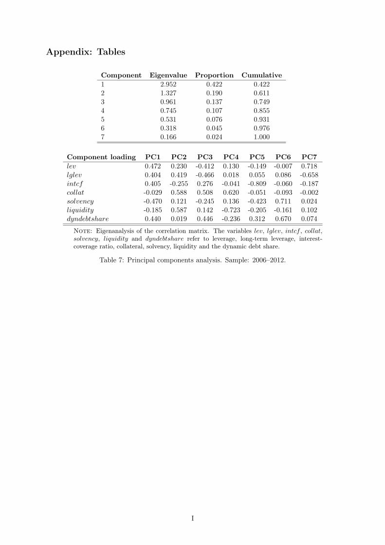
Appendix: Tables

Component Eigenvalue Proportion Cumulative

1 2.952 0.422 0.4222 1.327 0.190 0.6113 0.961 0.137 0.7494 0.745 0.107 0.8555 0.531 0.076 0.9316 0.318 0.045 0.9767 0.166 0.024 1.000

Component loading PC1 PC2 PC3 PC4 PC5 PC6 PC7

lev 0.472 0.230 -0.412 0.130 -0.149 -0.007 0.718lglev 0.404 0.419 -0.466 0.018 0.055 0.086 -0.658intcf 0.405 -0.255 0.276 -0.041 -0.809 -0.060 -0.187collat -0.029 0.588 0.508 0.620 -0.051 -0.093 -0.002solvency -0.470 0.121 -0.245 0.136 -0.423 0.711 0.024liquidity -0.185 0.587 0.142 -0.723 -0.205 -0.161 0.102dyndebtshare 0.440 0.019 0.446 -0.236 0.312 0.670 0.074

Note: Eigenanalysis of the correlation matrix. The variables lev, lglev, intcf , collat,solvency, liquidity and dyndebtshare refer to leverage, long-term leverage, interest-coverage ratio, collateral, solvency, liquidity and the dynamic debt share.

Table 7: Principal components analysis. Sample: 2006–2012.

I

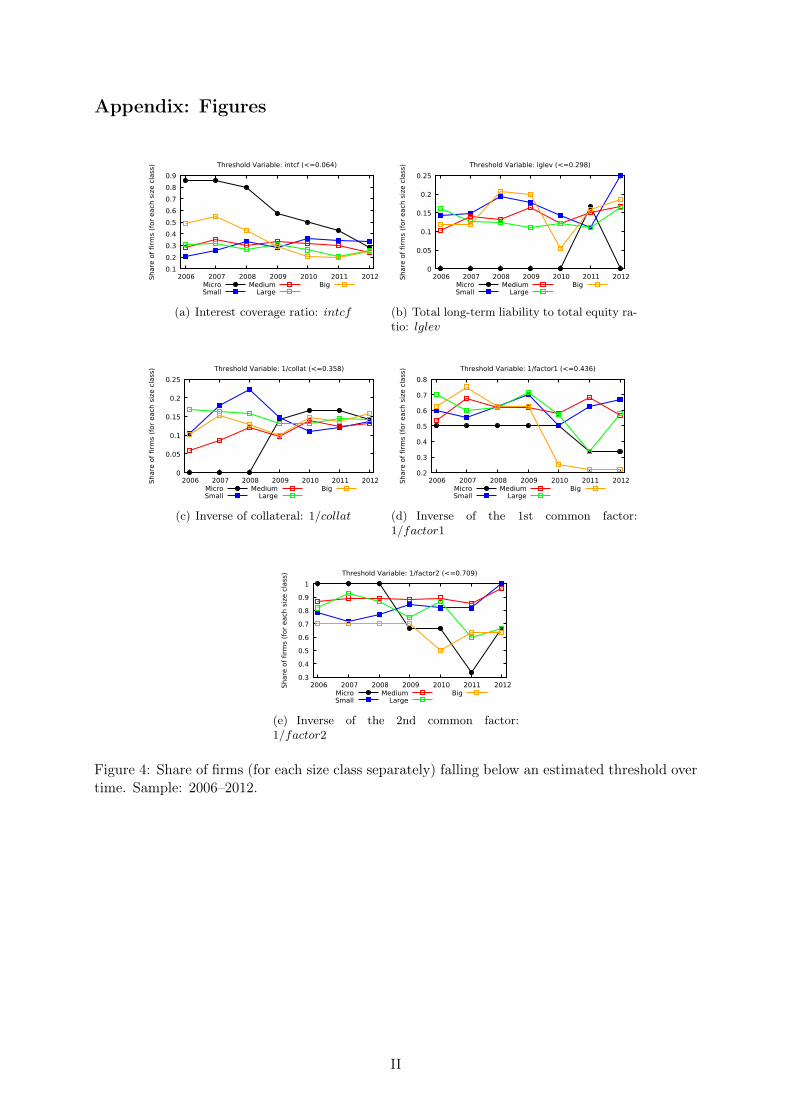
Appendix: Figures

0.1

0.2

0.3

0.4

0.5

0.6

0.7

0.8

0.9

2006 2007 2008 2009 2010 2011 2012Share

of

firm

s (

for

each s

ize c

lass) Threshold Variable: intcf (<=0.064)

MicroSmall

MediumLarge

Big

(a) Interest coverage ratio: intcf

0

0.05

0.1

0.15

0.2

0.25

2006 2007 2008 2009 2010 2011 2012Share

of

firm

s (

for

each s

ize c

lass) Threshold Variable: lglev (<=0.298)

MicroSmall

MediumLarge

Big

(b) Total long-term liability to total equity ra-tio: lglev

0

0.05

0.1

0.15

0.2

0.25

2006 2007 2008 2009 2010 2011 2012Share

of

firm

s (

for

each s

ize c

lass) Threshold Variable: 1/collat (<=0.358)

MicroSmall

MediumLarge

Big

(c) Inverse of collateral: 1/collat

0.2

0.3

0.4

0.5

0.6

0.7

0.8

2006 2007 2008 2009 2010 2011 2012Share

of

firm

s (

for

each s

ize c

lass) Threshold Variable: 1/factor1 (<=0.436)

MicroSmall

MediumLarge

Big

(d) Inverse of the 1st common factor:1/factor1

0.3

0.4

0.5

0.6

0.7

0.8

0.9

1

2006 2007 2008 2009 2010 2011 2012Share

of

firm

s (

for

each s

ize c

lass) Threshold Variable: 1/factor2 (<=0.709)

MicroSmall

MediumLarge

Big

(e) Inverse of the 2nd common factor:1/factor2

Figure 4: Share of firms (for each size class separately) falling below an estimated threshold overtime. Sample: 2006–2012.

II