Financial Innovation and New

Structured Products in the

Equity World

Dilip B. MadanRobert H. Smith School of Business

University of Maryland

CARISMA Event

7 City Learning

London

June 28 2007

OUTLINE

• Risk exposures of products.

• Supply side of structured products.

• Modelling the bid and ask prices.

Describing the Risks

• The structured products are contingent claims onthe paths of underliers and so they are exposed

to movements in the prices of these underlying

assets.

• They also embed many optionalities with respectto the paths of the underlying asset prices and can

in principle be hedged by positions in options.

• They are therefore exposed to the movements inthe option surface.

• They also deliver monies through time and thisexposes their values to interest rate risk and the

correlations between these and the underliers de-

termining the cash flows.

• Many of these risks can be managed by positionsin traded assets from time to time, as the expo-

sure detected is deemed undesirable and needs to

be mitigated.

• Of particular relevance in this context is productsthat build in what is called digital risk, where the

asset position required to mitigate the risk goes to

infinity and the risk can then not be realistically

managed.

• Yet another important feature is nonlinearity orconvexity/concavity of value which when sharp

requires further optionalities to build a hedge or

control the loss exposure.

Enumeration of Risks

• We may enumerate the risks as follows.

• From the underliers we have the

— The delta with respect to each underlier.

— The gamma with respect to each underlier in

case of convexity or concavity.

— The cross gamma or exposure to the second

order cross partial with respect to two asset

prices.

• From the option surface we have

— The level of volatilities

— The level of skews measured for instance as

the difference between the 90 − 110 impliedvolatilities.

— The convexity of the implied volatility curve.

— The volatility spread between longer and shorter

maturity options.

— The gammas with respect to each of the above

option surface risks in case of sharp convexities

or concavities.

∗ This leads to the· volgamma,

· skewgamma,

· convexitygamma, and

· the volspreadgamma.

• From the fixed income arena

— Exposure to the yield curve.

— Exposure to correlations between the under-

liers and interest rates.

Assessing the Risks

• We may value the product using a model cali-brated to the relatively more liquid surface of op-

tion prices and then we may shift the surface to

assess for example the surface risks.

• This is a complex calculation that is difficult todo for each product and each risk element.

• Somewhat cruder but helpful, is to understandthe risks in the components of the products, that

is the risk in each of the promised coupons with

their built in optionalities.

• For particular products we consider the exposureto volgamma, skewgamma and the convexity gamma.

Surface Exposures of Products

• We present with a view to illustrating option sur-face deltas and gammas the cliquet and reverse

cliquet volgamma and the ATM swing cliquet

skewgamma.

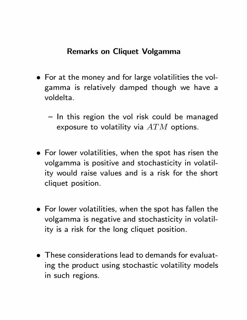
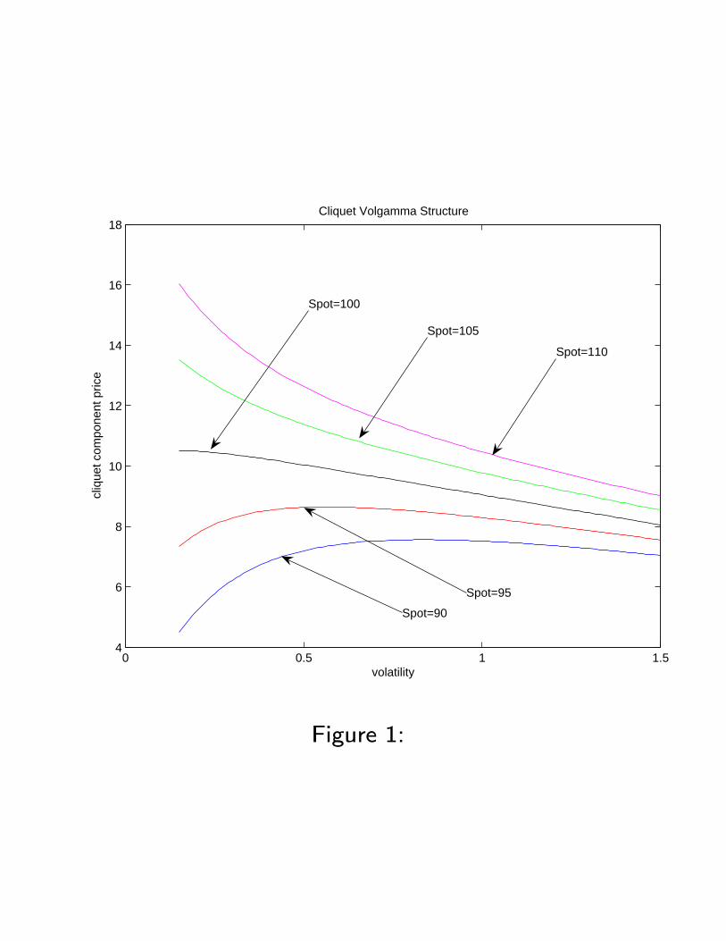
Remarks on Cliquet Volgamma

• For at the money and for large volatilities the vol-gamma is relatively damped though we have avoldelta.

— In this region the vol risk could be managedexposure to volatility via ATM options.

• For lower volatilities, when the spot has risen thevolgamma is positive and stochasticity in volatil-ity would raise values and is a risk for the shortcliquet position.

• For lower volatilities, when the spot has fallen thevolgamma is negative and stochasticity in volatil-ity is a risk for the long cliquet position.

• These considerations lead to demands for evaluat-ing the product using stochastic volatility modelsin such regions.

0 0.5 1 1.54

6

8

10

12

14

16

18

volatility

cliq

uet c

ompo

nent

pric

e

Cliquet Volgamma Structure

Spot=90

Spot=95

Spot=100

Spot=105

Spot=110

Figure 1:

• Additionally it is anticipated that option hedgesfor volatility may need to be rebalanced and the

costs for these must be anticipated.

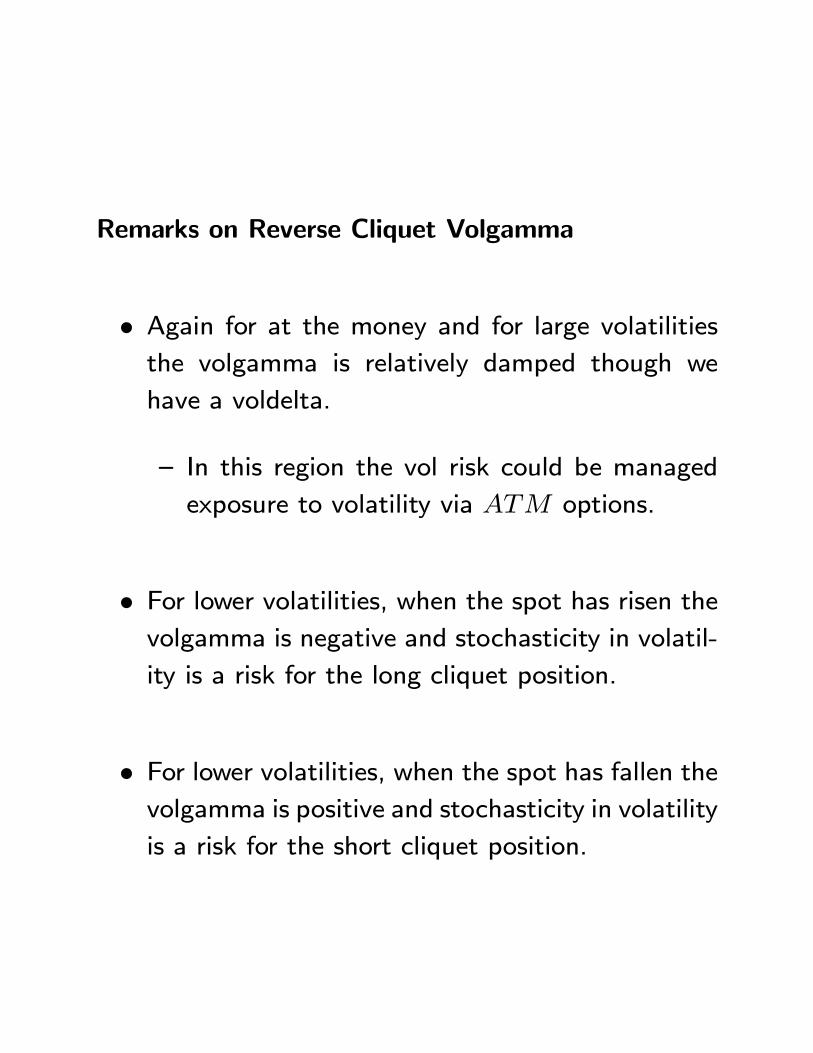
Remarks on Reverse Cliquet Volgamma

• Again for at the money and for large volatilitiesthe volgamma is relatively damped though we

have a voldelta.

— In this region the vol risk could be managed

exposure to volatility via ATM options.

• For lower volatilities, when the spot has risen thevolgamma is negative and stochasticity in volatil-

ity is a risk for the long cliquet position.

• For lower volatilities, when the spot has fallen thevolgamma is positive and stochasticity in volatility

is a risk for the short cliquet position.

0 0.5 1 1.52

4

6

8

10

12

14

16

volatility

Rev

erse

cliq

uet c

ompo

nent

pric

e

Reverse Cliquet Volgamma Structure

Spot=90Spot=95

Spot=100Spot=105 Spot=110

Figure 2:

Remarks of Swing Cliquet Skewgamma

• The presence of convexity in the value of theswing cliquet with respect to the skew suggests

that stochasticity in the skew may impact the

value of this claim upwards.

• Valuation of such claims under a stochastic skewmodel is then of some interest.

• Models of this type are now under construction.

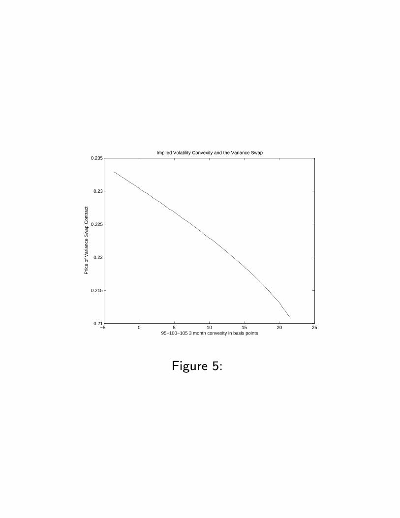
Marked to Market Risks of the Variance Swap

• The variance swap contract trades quite popularlyand options on volatility are beginning to trade.

The risk exposures of these contracts are of in-

terest as they are also used for covariance swap

contract construction.

• The well known robust hedge for the varianceswap is the short position in the log contract.

• This may easily be priced by any model fitting theoption smile at a single maturity with a known

characteristic function for the log price relative.

• We may also extract from the market the ATM

volatility, the 95-105 3 month skew and the 95-

100-105 3 month convexity.

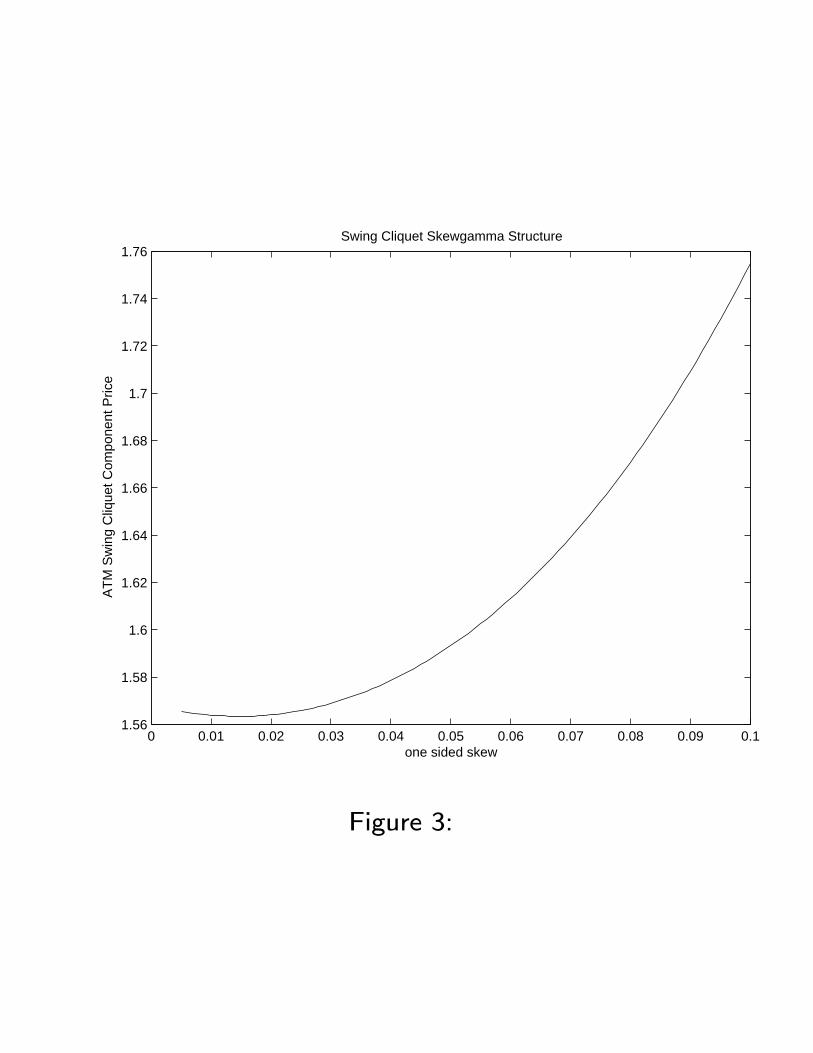
0 0.01 0.02 0.03 0.04 0.05 0.06 0.07 0.08 0.09 0.11.56

1.58

1.6

1.62

1.64

1.66

1.68

1.7

1.72

1.74

1.76

one sided skew

AT

M S

win

g C

lique

t Com

pone

nt P

rice

Swing Cliquet Skewgamma Structure

Figure 3:

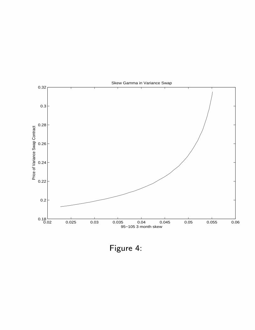
Skew gamma in variance swaps

• The presence of a skew gamma in the variance

swap contract is yet another reason for models

with stochastic skews.

0.02 0.025 0.03 0.035 0.04 0.045 0.05 0.055 0.060.18

0.2

0.22

0.24

0.26

0.28

0.3

0.32Skew Gamma in Variance Swap

95−105 3 month skew

Pric

e of

Var

ianc

e S

wap

Con

tract

Figure 4:

−5 0 5 10 15 20 250.21

0.215

0.22

0.225

0.23

0.235Implied Volatility Convexity and the Variance Swap

95−100−105 3 month convexity in basis points

Pric

e of

Var

ianc

e S

wap

Con

trac

t

Figure 5:

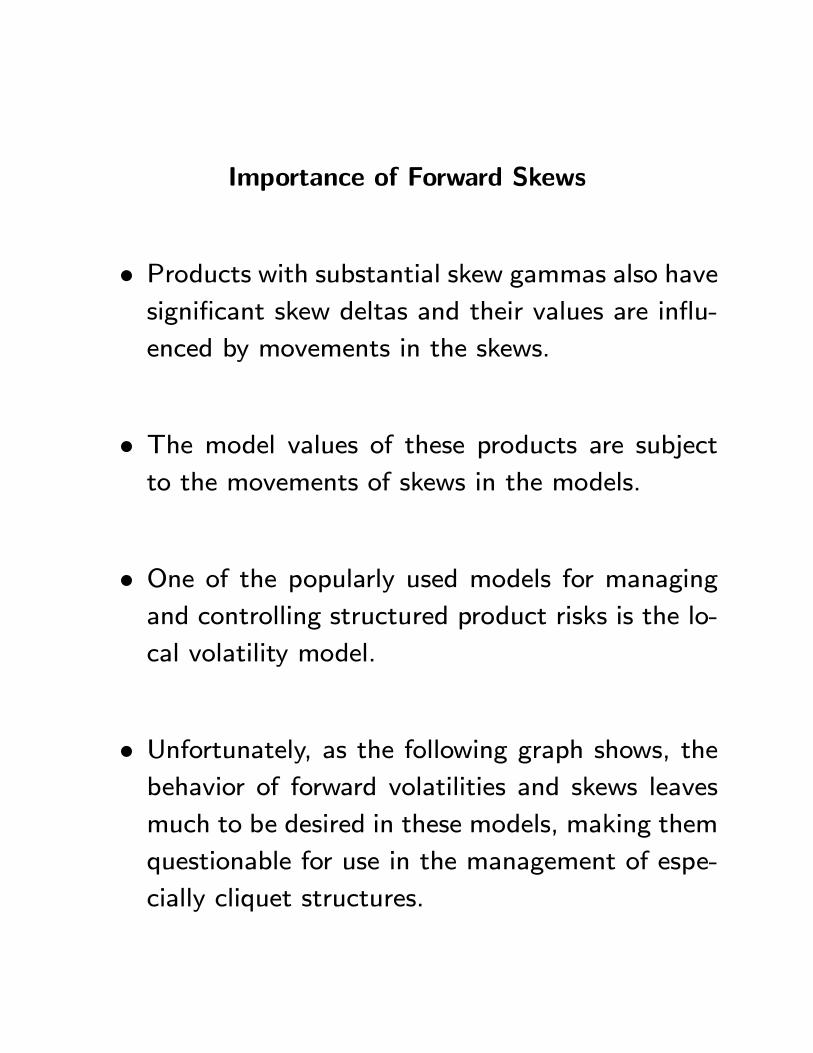
Importance of Forward Skews

• Products with substantial skew gammas also havesignificant skew deltas and their values are influ-

enced by movements in the skews.

• The model values of these products are subjectto the movements of skews in the models.

• One of the popularly used models for managingand controlling structured product risks is the lo-

cal volatility model.

• Unfortunately, as the following graph shows, thebehavior of forward volatilities and skews leaves

much to be desired in these models, making them

questionable for use in the management of espe-

cially cliquet structures.

• These considerations led to the development oflocal Levy models that better manage forward

skew evolution.

Cross Gamma Effects

• Structures involving Napoleonic features or de-pendencies on worst performers as the minimum

price across a set of names have a delta that is

primarily determined by the names that are cur-

rently the worst performer.

• When another name replaces these names as theworst performer, the primary delta effect switches

to the new asset.

• As a result, the delta with respect to the previ-ous worst performer can drop sharply without any

movement in its price but simply by the drop in

the value of the new worst performer.

• These effects are called cross gamma effects andfor certain products one needs to watch out for

these movements.

0.8 0.85 0.9 0.95 1 1.05 1.1 1.15 1.2 1.250.18

0.2

0.22

0.24

0.26

0.28

0.3Six Month Forward Start Implied Volatilities in Local Vol on SPX 20040706

Strike

Impl

ied

Vol

atili

ty

Six months out

2 years out

3 years out

4 years out

Figure 6:

Cross Gamma in Basket Option Trades

• Structured Products provided optionality over abasket of names may often be hedged by posi-

tions in the individual options. The result is a

value function that depends nonlinearly on both

the asset values.

• One may evaluate across the state space of as-set prices, the exposure of the delta hedged value

function to discover saddle point structures whereby

we have zero delta and positive gamma in each

direction so that the position looks good.

• However there may be a strong negative crossgamma with the consequence that if a pair of

prices moves in a certain direction then significant

losses are to be incurred.

• An eigen value analysis of the matrix of secondderivatives will reveal all the negative and positive

gamma directions.

• The hedged structure needs to be watchful ofthese directional gammas.

Structures Exposed to Digital Risk

• Sharp barrier clauses like knock outs or knock insof value on specific events lead to difficulties in

managing the risk near the barrier.

• It is best to cover these situations by option po-sitioning across the barrier event, as opposed to

relying on the delta hedging mechanisms.

• The positioning should be undertaken some whatin advance of the barrier to control the cost of

insurance purchase.

Correlation between Equity and Interest Rate Risks

• Equity Returns and interest rate movements gothrough periods of differing levels of correlation.

• A period of strong positive correlation has equitylinked notes making healthy payouts in higher in-

terest markets and this raises the value of the

payout to the investor.

• One may therefore wish to assess the value ofthe contract using a model that allowed for posi-

tive correlation between equity returns and inter-

est rates.

• Typically, if the cash flows are more bond likewith their volatility diminished, the correlation of

the timing with the interest rate environment gets

relatively more important.

• To the extent that equity volatility feeds into thepayout pattern the correlation effects with inter-

est rate movements get dominated.

• Particulary suited to such investigations are factormodels that are jointly driving the equity and the

instantaneous short rate.

Supply Side of Structured Products

• There are many risks to be understood, managedand priced into the ask price of structured prod-

ucts.

• How can we go about the production of liabilitiesincurred on the sale of a structured product.

• Clearly, to the extent we can take positions incurrent and future option market assets to cover

the liability, we have some understanding of how

to produce the structured product and what to

charge for it.

• Exact replication is however, unlikely and we needto determine how one may make the holding of

the residual an acceptable risk.

• These ideas lead to a stylised model for the de-termination of structured product ask, and if nec-

essary bid, prices.

The Relatively Liquid Hedging Assets

• We go back to viewing the structured productas a scenario contingent vector of payouts x =

(xs, s = 1, · · · ,M).

• Next we introduce traded assets whose prices areknown along the scenario paths and by financing

their prices we generate a matrix of zero cost cash

flows Y where Yjs is the present value cash flow

accessed by positioning in zero cost liquid asset j

on scenario s.

• These assets could include the financed purchaseof stock for some interval of time as well as the

financed purchase of current or forward starting

options held to maturity.

• If we adopt the hedge that takes the position αj

in liquid asset j then our residual cash flow is

α0Y − x0

• If this position is zero or nonnegative, it is clearlyacceptable.

• However, this is not likely to be the case.

Acceptable Risks

• Acceptable Risks have been effectively defined asa convex cone containing the positive orthant.

• Intuitively, if a sufficient number of counterpartiesvalue the gains in excess of the losses, then the

risk is acceptable.

• For practical purposes this amounts to the exis-tence of valuations that are probability times path

dissatisfaction weighted averages of the risky cash

flows, all which must be positive for a risk to be

accepted.

• Let B be the matrix of such valuation measures

used for testing acceptability. (See Carr, Geman,

Madan JFE 2002 for greater details).

• For the risk to be acceptable we must have(α0Y − x0)B ≥ 0

• It may be the case that such is not possible andso we add cash to the position, that is essentially

the price sought for the sale of the liability x.

• The smallest number a that rendersa+

³α0Y − x0

´B ≥ 0

is an admissible price for the sale of x coupled

with hedge α.

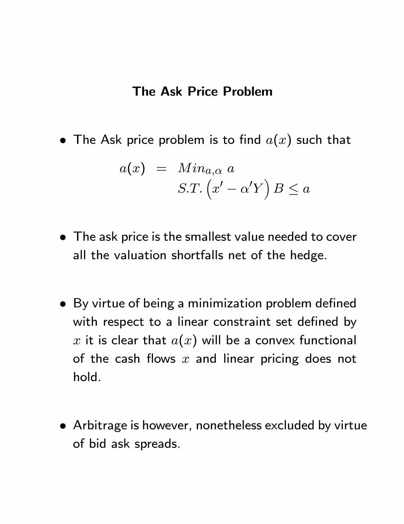
The Ask Price Problem

• The Ask price problem is to find a(x) such that

a(x) = Mina,α a

S.T.³x0 − α0Y

´B ≤ a

• The ask price is the smallest value needed to coverall the valuation shortfalls net of the hedge.

• By virtue of being a minimization problem definedwith respect to a linear constraint set defined by

x it is clear that a(x) will be a convex functional

of the cash flows x and linear pricing does not

hold.

• Arbitrage is however, nonetheless excluded by virtueof bid ask spreads.

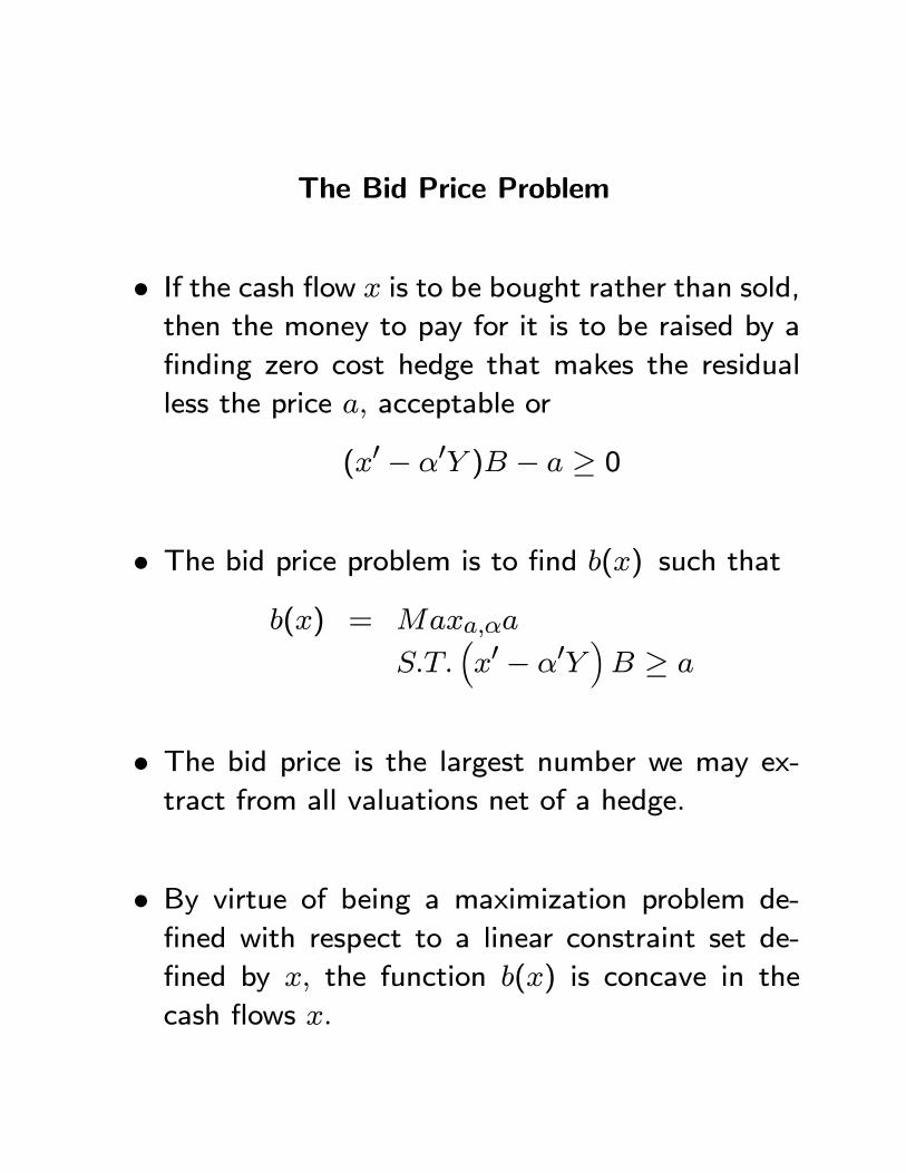
The Bid Price Problem

• If the cash flow x is to be bought rather than sold,

then the money to pay for it is to be raised by a

finding zero cost hedge that makes the residual

less the price a, acceptable or

(x0 − α0Y )B − a ≥ 0

• The bid price problem is to find b(x) such that

b(x) = Maxa,αa

S.T.³x0 − α0Y

´B ≥ a

• The bid price is the largest number we may ex-tract from all valuations net of a hedge.

• By virtue of being a maximization problem de-

fined with respect to a linear constraint set de-

fined by x, the function b(x) is concave in the

cash flows x.

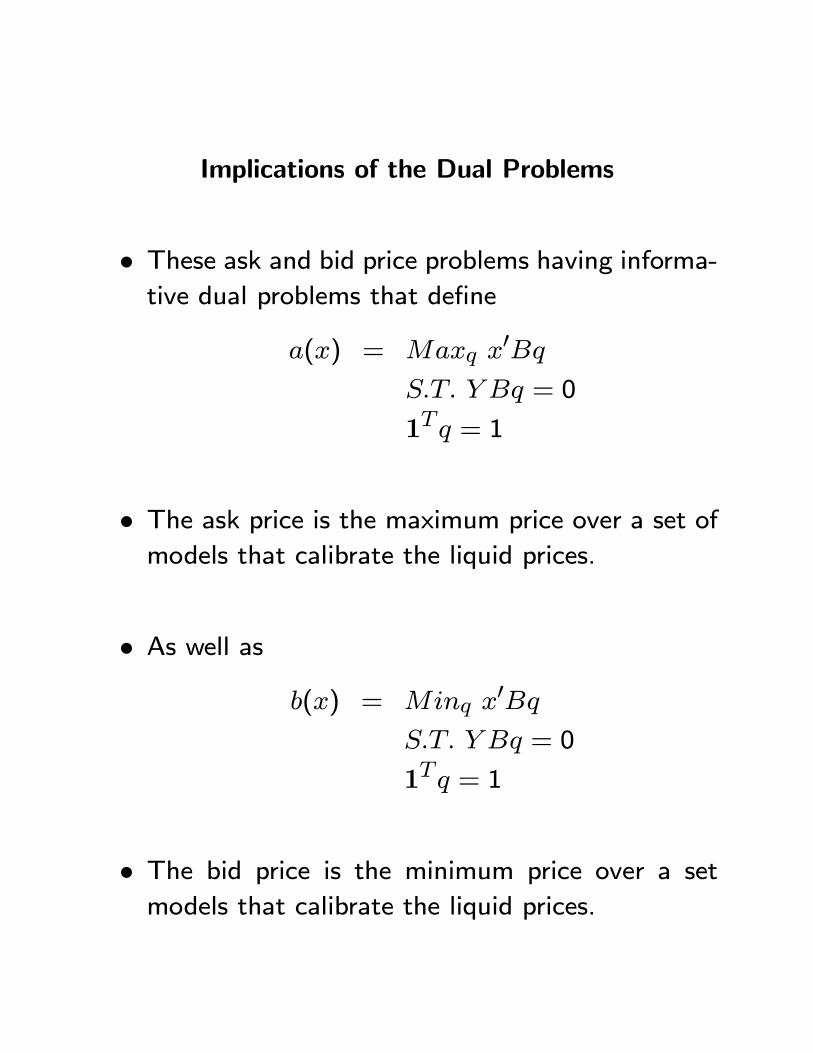
Implications of the Dual Problems

• These ask and bid price problems having informa-tive dual problems that define

a(x) = Maxq x0Bq

S.T. Y Bq = 0

1Tq = 1

• The ask price is the maximum price over a set of

models that calibrate the liquid prices.

• As well asb(x) = Minq x0Bq

S.T. Y Bq = 0

1Tq = 1

• The bid price is the minimum price over a set

models that calibrate the liquid prices.

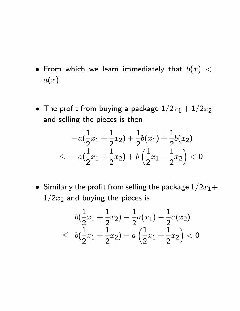
• From which we learn immediately that b(x) <

a(x).

• The profit from buying a package 1/2x1+ 1/2x2and selling the pieces is then

−a(1

2x1 +

1

2x2) +

1

2b(x1) +

1

2b(x2)

≤ −a(1

2x1 +

1

2x2) + b

µ1

2x1 +

1

2x2

¶< 0

• Similarly the profit from selling the package 1/2x1+1/2x2 and buying the pieces is

b(1

2x1 +

1

2x2)−

1

2a(x1)−

1

2a(x2)

≤ b(1

2x1 +

1

2x2)− a

µ1

2x1 +

1

2x2

¶< 0

Acceptability, Hedging, and Arbitrage

• Given a uniform definition or agreement on the

acceptability of risks, or agreement on the mea-

sures that test acceptability, one may define ac-

ceptable hedges that yield concave ask prices and

convex bid prices.

— Importantly, this structure excludes market par-

ticipants from exposure to arbitrage by coun-

terparties.

• Additionally, the differences generally observed inthe prices of structured products using vanilla op-

tion calibrated models are no evidence of model

risk, as none of these prices is a price.

— Their maximum is an ask price while their min-

imum is a bid price.

• Furthermore, it is a natural consequence of thetechnology of hedging to acceptability that dif-

ferent products are priced using different models.

— This is not an inconsistency, but just the recog-

nition that the ask price for different products,

seen as the maximum price over a set of cal-

ibrated models, attains this maximum at dif-

ferent models.

• Of course the fewer the set of risks that are ac-ceptable, the wider is the bid ask spread and the

less likely that there is a trading counterparty for

any particular product.

— Consensus over acceptability is attained as the

broad structure of models in use is eventually

widely disseminated.