Financial Flexibility: At What Cost??

Mark J. Garmaise and Gabriel Natividad∗

ABSTRACT

Firms strategically borrow in different locations. Approximately one quarter of Peruvian

companies with operations in multiple areas source their financing from more than one

province. Mining windfalls generate finance supply shocks leading to the provision of more

credit at lower average rates, and we show that firms exploit geographical financial flexibility

by concentrating their borrowing in booming locations. Firms are less likely to initiate

borrowing in new markets when their current borrowing provinces are thriving. The pursuit

of flexibility in borrowing markets, however, degrades a firm’s relationships with its existing

lenders, thereby heightening its risk of future financial distress.

*Garmaise is at UCLA Anderson (mark.garmaise@anderson.ucla.edu). Natividad is at Universidad de Piura

(gabriel.natividad@udep.pe).?We are grateful to the Superintendencia de Banca, Seguros, y AFPs and to Ministerio de la Produccion for

access to the data. We also thank audiences at New York University, Universidad de Montevideo, Universidad

de Piura and the Annual Conference of the Peruvian Central Reserve Bank for comments, and we thank

Guillermo Ramirez-Chiang, Jharold Montoya and Renzo Severino for valuable research assistance.

Achieving financial flexibility is a key policy goal for firms. Survey evidence (Graham and

Harvey 2001), theoretical models (e.g., Gamba and Triantis 2008) and empirical studies

(Denis 2011 provides an overview) have all emphasized the importance to corporations of

having ready and inexpensive access to credit. In this paper we examine one aspect of

optionality in financial choices: the ability of firms operating in multiple areas to strategically

focus their borrowing in thriving local markets. We show that firms do indeed choose to

borrow in their most prospering locales, where credit is plentiful and relatively inexpensive.

We also find, however, that the pursuit of geographic financial flexibility can come at a

cost. Firms that initiate borrowing in new flourishing markets neglect their existing banking

relationships and, as a result, experience higher risks of eventual financial distress. A firm’s

agility in accessing financing in different markets on attractive terms must therefore be

understood to carry the consequence of degrading important connections to their current set

of lenders.

We study a sample of Peruvian firms over the period 2001-2012. These firms have

business operations in multiple provinces. We first document that 25.5% of the firms borrow

in more than one province at some point during our sample period. Specifically, these firms

hold loans extended from bank branches located in different provinces. That is, we find that

for many quite small firms (the median number of employees at multi-province borrowers is

eight), seeking flexibility in the areas in which they borrow is an important aspect of their

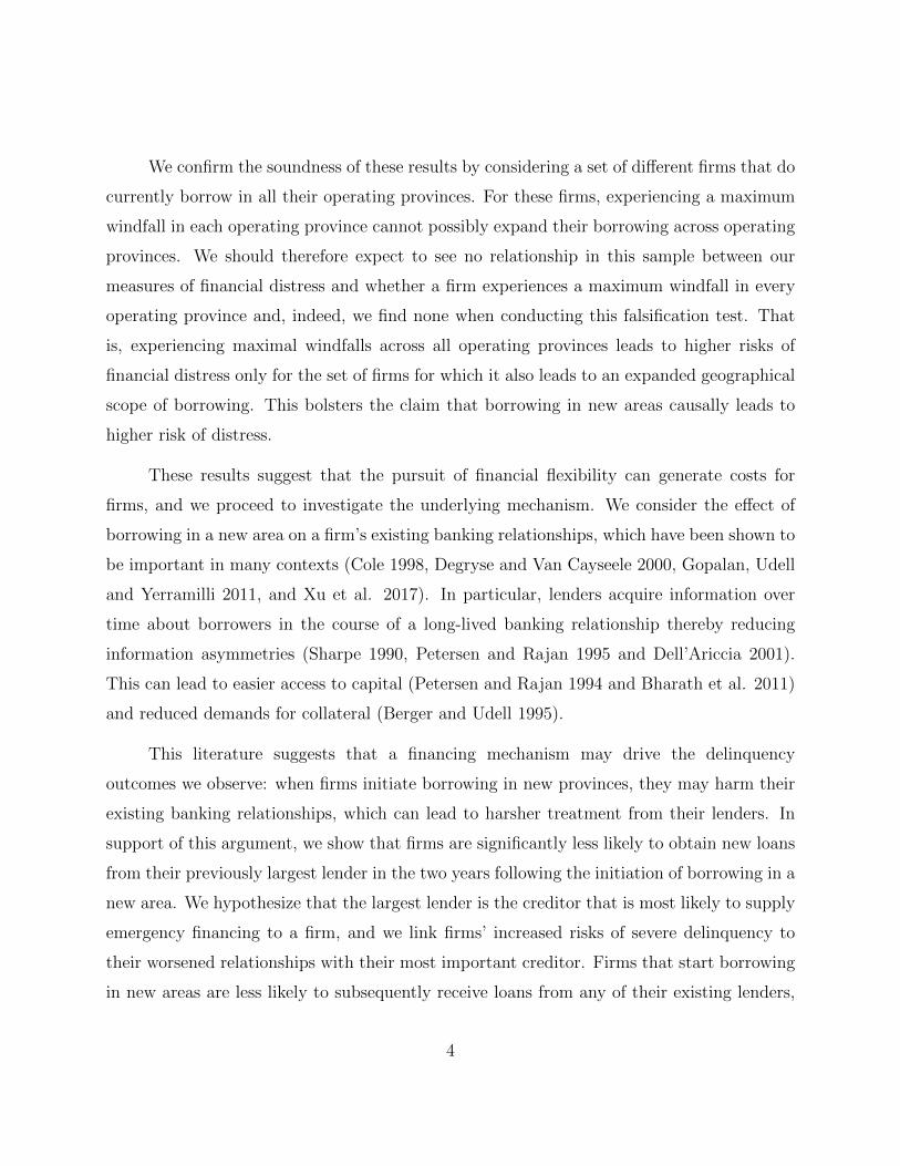
financial policy. Moreover, as displayed in Figure 1, total lending to multi-province borrowers

accounts for roughly 15%-25% of all commercial lending nationally. For firms that engage

in multi-location borrowing, only 50% of their financing comes from banks in the province

where the firm headquarters is situated.

Multi-location borrowing is not simply a firm strategy to gain access to a wider set

of banks. We find that more than 80% of multi-location borrowers take loans from a

bank outside their headquarters region that does, in fact, have a branch within the firms’

headquarters province. We also find no evidence that firms concentrate their most troubled

debt in banks in non-headquarters provinces.

1

Why, then, do firms borrow outside their headquarters regions? To better understand

the attractiveness of borrowing in different provinces, we explore the impact of changes in

commodity prices on the provision of credit. Peru is a natural resource-driven country and

mining is a critical sector. For each province we calculate local mining windfalls arising

from international commodity price changes multiplied by the mining production of these

commodities for all the mines located near the provincial centroid. We show that these

mining windfalls stimulate local borrowing booms for both single and multiple location firms

(across a variety of industries, not only in the mining sector), and we view them as generating

plausibly exogenous supply shocks to local financing conditions. Mining windfalls lead both

to a surge in the quantity of credit supplied and a reduction in the average interest rate

charged: a one standard deviation increase in the windfall increases the quantity of finance

supplied by 1.7% and reduces the interest rates on short-term debt by 24 basis points.

We study the drivers of multi-location borrowing by analyzing how it is influenced

by mining windfalls in different areas. We find that a one standard deviation increase in

the local mining windfall leads to a 5.4% increase in local borrowing, but a one standard

deviation increase in the mining windfall in other provinces generates a 4.3% decrease in local

borrowing. Firms thus appear to flexibly source their financing by borrowing in relatively

better-performing areas and reducing the credit they seek in distressed regions. This is

evidence that firm borrowing in one area serves as a substitute for borrowing in other regions.

We find that this substitution effect is concentrated in the firm’s existing bank relationships:

mining windfalls in other provinces lead to reduced borrowing from existing local lenders.

We analyze how firms widen their geographic financing options by studying their

decisions to initiate borrowing in new provinces in which they operate but do not currently

receive credit. Under our real options understanding of the role played by multi-location

borrowing, we should expect firms to start borrowing in new locations when the provinces

in which they are currently receiving financing are not prospering. On this view, the

attractiveness of borrowing in a new market will be determined by the most positive windfall

across a firm’s current borrowing provinces. We compare firms operating in the same province

2

that are currently unbanked in that province. We show that a one standard deviation increase

in the maximum windfall experienced by a firm across its existing borrowing provinces leads

to a 0.06% decrease in the probability of borrowing in the unbanked province, relative to

an average probability of 1.89% of initiating borrowing in a new province. The specification

for this test makes use of province-month-year fixed effects to control for any local demand

shocks. In other words, this result provides clear evidence that mining windfalls in a firm’s

borrowing provinces create finance supply shocks that have a strong influence on the firm’s

decision to initiate financing in a previously untapped area.

We document clear benefits of pursuing flexibility in the location of borrowing: a

greater supply of credit at a lower average price. What are the offsetting costs? We examine

this question by seeking a plausibly exogenous determinant of a firm’s decision to initiate

borrowing in a new area. We consider only the sample of firms that do not presently borrow in

all their operating provinces; these are firms that could initiate borrowing in a new operating

province. We argue that if a firm in this sample experiences a maximal monthly windfall over

the previous year in every one of its operating provinces, then it will certainly experience

a windfall in a province in which it did not previously borrow, and the firm is therefore

more likely to initiate borrowing in a new province. This firm will be exposed to attractive

borrowing conditions in new markets. We show that, controlling for headquarters province-

year-month fixed effects and for the maximum and average windfalls to which a firm is

exposed in its current borrowing provinces, it is indeed the case that firms that experienced

windfalls in all their operating provinces in the previous year are more likely to subsequently

initiate borrowing in a new province.

We therefore propose that experiencing a windfall in each operating province can serve

as an instrument for initiating borrowing in a new province. Using this instrument, we find

that firms that expand the set of provinces in which they borrow later experience more severe

loan delinquencies and are more likely to have loans become subject to judicial collection.

In other words, a causal effect of expanded geographical financial flexibility is an increased

risk of financial distress.

3

We confirm the soundness of these results by considering a set of different firms that do

currently borrow in all their operating provinces. For these firms, experiencing a maximum

windfall in each operating province cannot possibly expand their borrowing across operating

provinces. We should therefore expect to see no relationship in this sample between our

measures of financial distress and whether a firm experiences a maximum windfall in every

operating province and, indeed, we find none when conducting this falsification test. That

is, experiencing maximal windfalls across all operating provinces leads to higher risks of

financial distress only for the set of firms for which it also leads to an expanded geographical

scope of borrowing. This bolsters the claim that borrowing in new areas causally leads to

higher risk of distress.

These results suggest that the pursuit of financial flexibility can generate costs for

firms, and we proceed to investigate the underlying mechanism. We consider the effect of

borrowing in a new area on a firm’s existing banking relationships, which have been shown to

be important in many contexts (Cole 1998, Degryse and Van Cayseele 2000, Gopalan, Udell

and Yerramilli 2011, and Xu et al. 2017). In particular, lenders acquire information over

time about borrowers in the course of a long-lived banking relationship thereby reducing

information asymmetries (Sharpe 1990, Petersen and Rajan 1995 and Dell’Ariccia 2001).

This can lead to easier access to capital (Petersen and Rajan 1994 and Bharath et al. 2011)

and reduced demands for collateral (Berger and Udell 1995).

This literature suggests that a financing mechanism may drive the delinquency

outcomes we observe: when firms initiate borrowing in new provinces, they may harm their

existing banking relationships, which can lead to harsher treatment from their lenders. In

support of this argument, we show that firms are significantly less likely to obtain new loans

from their previously largest lender in the two years following the initiation of borrowing in a

new area. We hypothesize that the largest lender is the creditor that is most likely to supply

emergency financing to a firm, and we link firms’ increased risks of severe delinquency to

their worsened relationships with their most important creditor. Firms that start borrowing

in new areas are less likely to subsequently receive loans from any of their existing lenders,

4

but the effect is most severe for the largest initial lender. The initiation of borrowing in

a new province is also associated with a significantly higher risk of permanent relationship

termination with both the main initial lender and with any of their existing creditors. Firms

that achieve geographical borrowing flexibility attain access to financing opportunities in

multiple areas, but we show that this comes at the cost of degraded relationships with their

previous lenders and heightened risks of default.

We examine alternative mechanisms that may explain the link we find between

borrowing in a new province and subsequent delinquency. First, we consider whether the

future distress of firms that borrow in new areas is potentially linked to the exposure of

their new lenders to cycles in the mining industry. Even when including fixed effects for the

set of lenders from which a firm borrows over the next 24 months, however, we continue to

find that borrowing in a new area leads to higher delinquency risk. This indicates that the

composition of lenders does not drive our main results. Second, we also find that controlling

for differences in the means and standard deviations of the windfalls experienced by firms

does not affect our findings. This suggests that it is specifically the experience of having

a windfall in each operating province and thereafter initiating borrowing in a new province

that leads to future delinquency, not a factor arising from the general pattern of windfalls.

It is the specific mechanism of maximum windfalls realized in each operating province

that leads to borrowing in a new province and future delinquency, not whether the firm

experiences broadly positive or highly time varying windfalls.

Third, we explore whether negative future outcomes may be driven by poor investment

choices by firms that experience maximum windfalls in all their operating provinces. We find,

however, that even when controlling for the future level of delinquency, a firm that initiates

borrowing in a new area is more likely to be subjected to future judicial collection by its

lenders. This is evidence of harsher treatment, conditional on performance, by lenders.

Moreover, we also create comparison samples of firms that borrow in all their operating

provinces and those that do not that are matched firm-by-firm in their set of operating

5

provinces and overall debt levels. Even for these highly matched samples of firms that

experience the same windfalls, we find that maximum windfalls in each province lead to

worse future outcomes only for the firms that can initiate borrowing in a new province (i.e.,

those for which the financing mechanism is operative). For example, we find that initiating

borrowing in a new region leads to a 6.2% increase in the probability of having debt enter

judicial status. This may be compared to the 9% difference in the average frequency of

judicial status loans between the lowest and highest GDP growth years in our sample. These

matched sample tests show that our results do not arise from comparing firms that experience

varying shocks that propel different investment strategies: the key mechanism driving future

delinquency is borrowing in a new area.

If banking relationships are important for the information they provide to lenders,

we should expect to see that the disruption of these relationships is more costly for

informationally opaque firms. In particular, effects should be more severe for firms that have

low levels of tangible assets and for firms that are younger. This is indeed what we find: the

link between initiating borrowing in a new province and future deliquency is strongest for

firms with low asset to sales ratios and for firms that have relatively short histories in the

formal financial sector.

Our findings describe the importance of expanding the geographical locus of borrowing

as a central flexibility goal of financial policy for a wide class of firms including some rather

small businesses. Our work complements research that has emphasized the role of flexibility

in determining firms’ cash holdings (Faulkender and Wang 2006 and Ang and Smedema

2011), debt policies (Kahl et al. 2008, DeAngelo, DeAngelo and Whited 2011, Denis and

McKeon 2011 and DeAngelo, Goncalves and Stulz 2017) and equity payouts (Jagannathan,

Stephens and Weisbach 2000, Hoberg, Phillips and Prabhala 2011 and Kumar and Vergara-

Alert 2018).

Our study also relates to work depicting the strategic borrowing of multinational firms

across a variety of countries, with the level of within-country borrowing dependent on features

6

of the local financing environment (Desai, Foley and Hines 2004 and Jang 2017). Our study,

by contrast, considers multi-province borrowing by small and medium-sized firms active in

only one country with a broadly uniform regulatory environment. Moreover, we introduce the

idea that seeking geographic financial flexibility can damage existing banking relationships

and lead to higher risk of financial distress, a cost that has not been emphasized in previous

work.

Previous work has considered a firm’s choice between one or multiple sources of

financing (e.g., Detragiache, Garella and Guiso 2000). Our emphasis, by contrast, is on

studying where, rather than from whom, a firm borrows; we are interested in the influence of

credit conditions in different areas on the locus of financing. Our results showing that multi-

location firms borrow in healthier credit markets suggest that these firms may play a role in

mitigating the impact of regional financial shocks (Samolyk 1994) on other borrowers. Multi-

location firms tend to seek less financing in markets that are struggling, thereby leaving the

scarce capital in these areas for the single-location firms that operate there. Our results also

point to the importance of regional credit competition by banks (Rice and Strahan 2010 and

Dou, Ryan and Zou 2018) to attract the borrowing of multi-location firms; money centers

may have a negative impact on the financial development of nearby locales. These types

of economic geographical analyses are not the focus of the single versus multiple banking

relationship literature.

Our work complements prior research describing the impact of local shocks on the

lending activities of banks (Gilje, Loutskina and Strahan 2016 and Bustos, Garber and

Ponticelli 2016). Unlike these papers, we focus on firms rather than banks. We document

a different effect: the banking papers show that a positive local shock leads banks to lend

more in other areas, whereas we find that these shocks lead multi-location firms to borrow

less elsewhere. In some sense these two forces are in tension and have opposing effects on the

location of borrowing. The interplay of bank lending and firm borrowing decisions across

different geographies can thus be rather complex.

7

Our results documenting and analyzing multi-location lending also have connections

to the literature on internal capital markets. We examine geographical patterns in financing

provided by banks while internal capital markets research has largely concentrated on

investment decisions (Ozbas and Scharfstein 2010), the internal allocation of capital to

divisions and internal capital transfers within firms (Buchuk et al. 2014). The idea that

internal capital markets allow firms to engage in winner-picking by investing in the most

attractive division (Stein 1997, Matsusaka and Nanda 2002 and Ersahin et al. 2016) resonates

with our argument that multi-location borrowing generates a real option to borrow in the

most prosperous region. We study firms borrowing in different markets rather than borrowing

by multiple business units or subsidiaries of large firms (Kolasinski 2009). We differ from

the internal capital markets literature in both our emphasis on the geographic real option in

financing and in our study of the relationship costs of borrowing in multiple areas.

Our findings contribute to the growing understanding that flexibility is a central

objective of corporate financial policy. We emphasize, however, that flexibility is a multi-

dimensional attribute. Firms that obtain greater geographical flexibility by borrowing in

more local markets may, at the same time, degrade existing creditor relationships and thereby

impair their ability to borrow in times of need.

1 Data

We analyze monthly business bank loan data from Peru for the period January 2001-June

2012. The data are obtained from Superintendencia de Banca, Seguros, y AFPs (SBS) and

are labeled the RCD (Reporte Crediticio de Deudores) database. For each Peruvian financial

institution, the database includes the monthly loan balances of every business borrower

regardless of its size. For our study, we exclude firms that throughout their whole history

are recorded by SBS as only receiving micro-credit. The RCD includes information about the

financial institution branch’s province were the loan was granted. There are 196 provinces

8

in Peru.

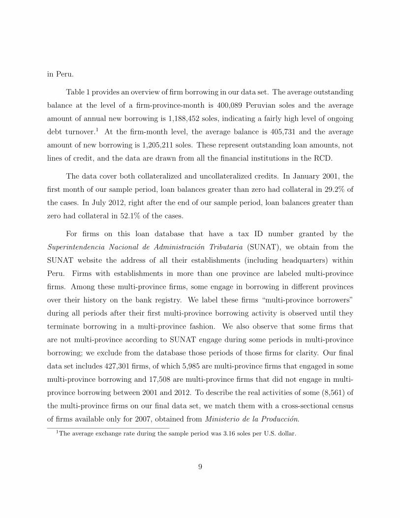
Table 1 provides an overview of firm borrowing in our data set. The average outstanding

balance at the level of a firm-province-month is 400,089 Peruvian soles and the average

amount of annual new borrowing is 1,188,452 soles, indicating a fairly high level of ongoing

debt turnover.1 At the firm-month level, the average balance is 405,731 and the average

amount of new borrowing is 1,205,211 soles. These represent outstanding loan amounts, not

lines of credit, and the data are drawn from all the financial institutions in the RCD.

The data cover both collateralized and uncollateralized credits. In January 2001, the

first month of our sample period, loan balances greater than zero had collateral in 29.2% of

the cases. In July 2012, right after the end of our sample period, loan balances greater than

zero had collateral in 52.1% of the cases.

For firms on this loan database that have a tax ID number granted by the

Superintendencia Nacional de Administracion Tributaria (SUNAT), we obtain from the

SUNAT website the address of all their establishments (including headquarters) within

Peru. Firms with establishments in more than one province are labeled multi-province

firms. Among these multi-province firms, some engage in borrowing in different provinces

over their history on the bank registry. We label these firms “multi-province borrowers”

during all periods after their first multi-province borrowing activity is observed until they

terminate borrowing in a multi-province fashion. We also observe that some firms that

are not multi-province according to SUNAT engage during some periods in multi-province

borrowing; we exclude from the database those periods of those firms for clarity. Our final

data set includes 427,301 firms, of which 5,985 are multi-province firms that engaged in some

multi-province borrowing and 17,508 are multi-province firms that did not engage in multi-

province borrowing between 2001 and 2012. To describe the real activities of some (8,561) of

the multi-province firms on our final data set, we match them with a cross-sectional census

of firms available only for 2007, obtained from Ministerio de la Produccion.

1The average exchange rate during the sample period was 3.16 soles per U.S. dollar.

9

We also employ information on the geocoded location and monthly production of mines

in Peru. The Ministerio de Energıa y Minas website supplies information on the production

and location of all 918 mining concessions between 2001 and 2012 that produced the leading

minerals of Peru (i.e., cadmium, copper, gold, iron, lead, molybdenum, silver, tin, tungsten,

and zinc), which is enhanced with geocoding tools obtained from Instituto Geologico, Minero

y Metalurgico. We employ that geocoded information to match the centroid of each province

in Peru with all mines within a certain distance in miles, as we describe in Section 2. Finally,

international end-of-month prices on each mineral produced by Peruvian mines are obtained

from Bloomberg.

2 Empirical Specification

We begin our empirical analysis with an examination of the frequency of multi-province

borrowing. We also provide a description of the financing patterns of multi-province

borrowers, illustrating where they borrow and the types of lenders from which they receive

credit.

We next turn to a causal analysis of the motivation for multi-province borrowing. We

make use of natural resource price changes in order to examine the impact of exogenous

shocks on the borrowing behavior of our firms. Mining is a large and important sector in

Peru (e.g., Sinnott, Nash and de la Torre 2010), and natural resource price changes are

likely to have broad economic effects. These price changes may also be regarded as plausibly

exogenous for almost all firms, as metal prices are determined at the international level.

For every mine j, we denote the month t − 1 production of metal k by that mine by

qj,k,t−1. The average price of metal k in month t− 1 is given by pk,t−1. For each mine every

month we define

10

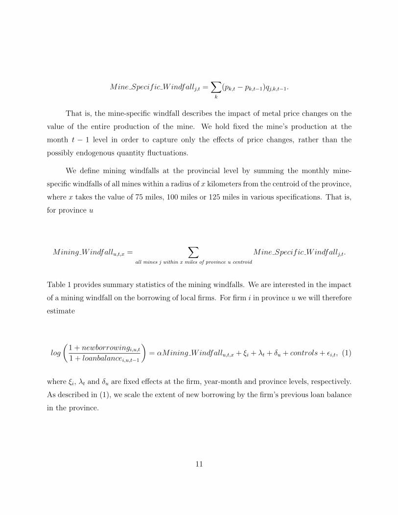
Mine Specific Windfallj,t =∑k

(pk,t − pk,t−1)qj,k,t−1.

That is, the mine-specific windfall describes the impact of metal price changes on the

value of the entire production of the mine. We hold fixed the mine’s production at the

month t − 1 level in order to capture only the effects of price changes, rather than the

possibly endogenous quantity fluctuations.

We define mining windfalls at the provincial level by summing the monthly mine-

specific windfalls of all mines within a radius of x kilometers from the centroid of the province,

where x takes the value of 75 miles, 100 miles or 125 miles in various specifications. That is,

for province u

Mining Windfallu,t,x =∑

all mines j within x miles of province u centroid

Mine Specific Windfallj,t.

Table 1 provides summary statistics of the mining windfalls. We are interested in the impact

of a mining windfall on the borrowing of local firms. For firm i in province u we will therefore

estimate

log

(1 + newborrowingi,u,t1 + loanbalancei,u,t−1

)= αMining Windfallu,t,x + ξi + λt + δu + controls+ εi,t, (1)

where ξi, λt and δu are fixed effects at the firm, year-month and province levels, respectively.

As described in (1), we scale the extent of new borrowing by the firm’s previous loan balance

in the province.

11

3 Results

3.1 Which Multi-province Firms Engage in Multi-province

Borrowing?

We begin with a general description of some of the differences between multi-province firms

that engage in multi-province borrowing and those that do not. For this description we

use the cross-sectional characteristics only of those firms covered by the 2007 Census. In

Table 2, Panel A we provide summary statistics on both multi-province and single-province

borrowers.

Two patterns stand out. First, the multi-province borrowing firms tend to be older

and larger (in terms of sales, employees, fixed assets and inventory) than multi-province

firms that borrow only in a single province. (Overall, many of these firms are quite small,

as the untabulated median number of employees for multi-province borrowers is eight and

for single-province borrowers is six.) Thus, one potential argument is that multi-province

borrowing is part of the development process of a firm as it ages and expands. There may

be fixed costs of borrowing in multiple regions that firms are only willing to bear once they

reach a certain minimum size. Second, multi-province borrowers are not more profitable, nor

are their operating units more distant from each other. Table 2, Panel B provides summary

statistics of multi-province borrowing by sector using all firms on the loan registry. There

is some variation across sectors in the frequency of multi-province borrowing, but it is not

uncommon in any sector.

3.2 Borrowing Patterns of Multi-province Borrowing Firms

In Table 3 we describe the broad financing policies for the set of firms with any history of

financing in multiple provinces using the credit registry. Many of these firms engage in multi-

province borrowing on an on-going basis: in any given month, there is a 57% probability of

12

multi-province borrowing, most often in 2 provinces. We find that new borrowing is common

in both HQ (headquarters) and non-HQ provinces, and in both provinces with the largest

outstanding loan balances for a firm and in other borrowing provinces. In other words, for

these firms, multi-province borrowing is frequent and found across a variety of jurisdictions.

Borrowing is not dramatically concentrated in HQ provinces: firm borrowing in HQ

provinces is on average only 50% of the firm total. The province in which a firm has its

largest outstanding balance is responsible on average for 81% of total firm borrowing, and

this is the HQ province in 52% of cases. Multi-province borrowing does not simply arise from

spillovers across neighboring provinces: considering the sample of multi-province borrowers

borrowing across exactly two provinces, we find that in only 14% of these firms does the

borrowing take place in adjacent provinces. For this group of firms, the average distance

between the centroids of their provincial borrowing locations is 238 miles.

Firms rarely borrow from the same bank in multiple locations; only 1% of multi-

province borrowers have same-bank and different-province debt in a given month. That is,

firms are borrowing in multiple locations from different banks. This suggests the possibility

that multi-province borrowing is motivated by a desire on the part of firms to get access

to new lenders who are only present in other locations. This hypothesis, however, is not

supported by the data: when firms borrow in non-HQ or non-largest debt provinces, the

banks providing these loans also do business in the HQ or largest-debt province 82% of the

time.

Are banks perhaps concentrating their troubled (delinquent) loans in one province

of the firm? We do not find much evidence for this. For both HQ and non-HQ debt,

the share that is troubled is 9%. The largest borrowing province has a troubled share of

8.33% compared to 9.96% for the non-largest province. The latter difference is statistically

significant at the 1% level but not large in magnitude.

The broad picture that emerges from these descriptive statistics is that multi-province

borrowing is a common practice in our sample of firms that is used by these firms to borrow

13

from multiple banks, even when they have access to the same set of banks in their HQ

provinces.

3.3 Mining Windfalls and the Quantity of Borrowing

In order to better understand the causal drivers of multi-province borrowing, we examine

how this borrowing responds to local shocks to the supply of finance. As described in Section

2, we estimate mining windfalls in different provinces and trace their impact on borrowing.

We emphasize here that our sample consists of firms from a variety of industries, not just

mining firms. In a resource-driven economy like Peru’s, mining windfalls may be expected

to affect a broad spectrum of firms.

The first question is whether mining windfalls have any impact on local borrowing. We

begin with an analysis of the quantity of lending that is supplied. To provide evidence on

this, we estimate equation (1) by regressing for each firm the log of one plus its new local

borrowing, scaled by the log of one plus its previous total local loan balance, on the local

mining windfall, firm, province and year-month fixed effects and a control for the province

population in the previous year. We begin by considering the sample of all firms –regardless of

whether they operate in one or multiple provinces– and we include in the windfall calculation

all mines within 100 miles of each provincial centroid. For multi-province firms, we treat

local borrowing in each province as a separate observation. We find, as shown in the first

column of Table 4, that the local mining windfall has a positive and significant impact on

firm borrowing (coefficient=1.156 and t-statistic=2.41); we double cluster standard errors

at both the province and year-month levels. A one standard deviation increase of 0.014 in

the mining windfall increases a firm’s borrowing by 1.7%. For an average firm, this results

in approximately 20,200 new soles in borrowing. This is evidence that metal price increases

lead to greater local financing.

Our main focus is on multi-province borrowing firms, so we split the sample into single-

province borrowers (firms that throughout the sample period borrow only in one province)

14

and multi-province borrowers. In the second column of Table 4 we show that single-province

firms borrow more when subject to a positive mining windfall (coefficient=1.085 and t-

statistic=2.13). In the third and fourth columns of the table we show that this conclusion is

robust to including mines within 75 miles of provincial centroids, but that the effects dampen

with distance and become statistically insignificant when including mines within 125 miles

of provincial centroids. In the fifth column of Table 4 we show that multi-province firm

borrowing is also sensitive to local mining windfalls (coefficient=2.290 and t-statistic=1.76).

Results in the sixth and seventh columns of Table 4 show that for multi-province borrowers

as well, we find a positive effect on borrowing of windfalls affecting mines within 75 miles

of provincial centroids and an insignificant effect of windfalls affecting mines with 125 miles

of provincial centroids. Table 4 establishes that windfalls affecting nearby mines lead to an

increased provision of financing to local firms.

3.4 Mining Windfalls and the Cost of Borrowing

In order to show that mining windfalls generate a finance supply shock, rather than simply

stimulate the demand for borrowing by local firms, we now turn to an analysis of the cost

of borrowing. Our data do not provide loan-level interest rates, but we do have access

to average lending rates at the bank-currency-month level. (Currencies of originations are

Peruvian soles and U.S. dollars.) For each bank every month we find the weighted average

mining windfall that it experiences across all of its lending provinces, using as weights the

amount of lending undertaken by the bank in each province. We regress a bank’s current

average lending rate over the subsequent twelve months on its weighted average mining

windfall, and we include as controls a currency dummy, bank fixed effects and year-month

fixed effects.

We begin by considering commercial interest rates on loans of maturity of 1 year or

less. As shown in the first column of Table 5, we find that a bank’s weighted average mining

windfall has a negative and significant effect (coefficent =-0.175 and t-statistic=-2.35) on

15

the average interest rates that it charges. Banks making loans in areas that benefit from

positive mining windfalls tend to charge lower interest rates to their commercial customers

over the next year. A one standard deviation increase of 0.0139 in the weighted average bank

mining windfall is associated with a reduction of 0.24 percentage points (i.e., 24 basis points)

in the average interest rate. In the second column of Table 5, we show that an increase in

the weighted average mining windfall also leads to a reduction in the average rate that a

bank charges on its commercial loans with maturity exceeding 1 year (coefficent =-0.223 and

t-statistic=-2.74).

These results and those described in Table 4 show that mining windfalls lead to reduced

local interest rates and an increase in local borrowing. These combined findings provide clear

evidence that the primary effect of a mining windfall is to generate a positive shock to the

supply of local finance.2 We now explore how multi-province borrowers exploit the effects of

windfalls on the financing environment.

3.5 Multi-province Borrowing

The results described in Tables 4 and 5 establish that mining windfalls lead to local finance

supply shocks for both single- and multi-province borrowing firms. Our main interest is

in the financing strategies of multi-province borrowers. In particular, what impact does a

mining windfall affecting one province of a multi-province firm have on its borrowing in

other provinces? There are two natural hypotheses. The first is that windfalls generate

local financing surpluses and these surpluses strengthen multi-province firms as a whole and

enable them to borrow more in other regions, as well. Under this hypothesis, windfalls in any

area in which the multi-province firm operates and borrows should lead to greater financing

in other provinces, as well.

The second hypothesis is that firms have relatively stable demand for financing and

2We provide further evidence in Section 3.6 below on the supply impact of mining windfalls on localborrowing.

16

that they borrow strategically in different markets to fulfill that demand. If one province in

which a firm is active receives a mining windfall generating a local financing surplus then

the firm will reduce its borrowing in other provinces.

We test these hypotheses by regressing for each multi-province borrowing firm the log

of one plus its new local borrowing, scaled by the log of one plus its previous total local loan

balance, on the local mining windfall, the average mining windfall in the other provinces

in which the firm borrows, firm-year fixed effects and the previous controls. The result,

displayed in the first column of Table 6, is that local borrowing increases in the local mining

windfall (coefficient=3.89 and t-statistic=4.12) and decreases in the average windfall in the

other provinces in which the firm borrows (coefficient=-2.58 and t-statistic=-1.93). Standard

errors are clustered at the province and firm-month levels. A one standard deviation increase

in the local mining windfall leads to a 5.4% increase in local borrowing, and a one standard

deviation increase in the mining windfall in other provinces generates a 4.3% decrease in

local borrowing.

The negative and significant coefficient on the average windfall in a firm’s other

provinces is clear support for the second hypothesis discussed above; when a firm experiences

a local financing surplus in one province, it reduces its borrowing in other areas. Multi-

province borrowing firms make use of flexibility in the location of their financing, borrowing

opportunistically in the provinces subject to positive shocks.

How do firms exploit local financing surpluses? Specifically, do they proceed by

expanding existing financing relationships or by initiating new relationships in areas

experiencing windfalls? We split each firm’s new financing into new financing received from

banks with which the firm has a pre-existing relationship and new financing received from

banks from which the firm had not borrowed before. As displayed in the second and third

columns of Table 6, we find that new financing from existing relationships increases in the

local windfall and decreases in the average windfall of other borrowing provinces, while

new financing from new relationships increases in the local windfall but is not significantly

17

related to other province windfalls. The spillover effect on local borrowing of mining windfalls

in other provinces is thus found exclusively for financing provided through the channel of

existing relationships. We also find, as shown in Table A.1 in the Appendix, that the

strongest spillover effects of windfalls in other areas are exhibited in the province that

currently supplies the largest share of a firm’s overall debt. Substitution thus mainly occurs

through the channel of existing relationships in areas in which the firm already has extensive

borrowing.3

The overall picture that emerges from Table 6 is that multi-location firms borrow more

in provinces subject to positive shocks and reduce their lending from existing relationships

when the local shocks are negative and other provinces are prospering. Multi-location firms

create flexibility in the geography of their financing through changes in the amounts borrowed

from the firm’s lenders in different areas. The pursuit of flexibility by multi-location firms

may be beneficial to single-location companies. Ill-fated regions may be subjected to negative

credit shocks that can hinder local development (Samolyk 1994). We have shown that

multi-location firms shift their borrowing from markets that are not performing well, which

may thereby leave more of the limited capital in these floundering regions to single-location

borrowers.

3.6 Initiating Multi-Province Firms’ Borrowing in Existing

Operating Provinces

The results presented in Table 6 show that multi-province borrowing firms exploit

geographical financial flexibility, borrowing more in the provinces that are subject to

relatively positive shocks. This suggests that firms opportunistically seek out the best

environments for borrowing. If that is true, then it will be primarily the firm’s areas with

3In Table A.1 in the Appendix we show that the sensitivity of local borrowing to other province windfallsis not related to a province’s banking density (defined as the total number of banks operating in a provincedivided by the total number of banks in the country).

18

the most positive shocks that are the ones determining the changes in its financing strategy.

In other words, a key determinant of a multi-province firm’s borrowing practices should be

the greatest mining windfall in all the provinces in which it borrows. In this section we test

this hypothesis by considering whether a multi-province firm’s decision to initiate banking

in a new province is influenced by its maximum windfall.

We consider the set of firms with operating branches in multiple provinces that are

currently not borrowing in at least one of those provinces. For the set of unbanked firm

locations, we ask whether the probability of initiating new borrowing in that province is

related to the highest windfall experienced in the firm’s existing set of borrowing provinces.

We regress an indicator for initiating new borrowing in the unbanked province in the next

12 months on the maximum windfall in any of the firm’s current borrowing provinces, and

we include firm and province-year-month fixed effects as controls.

We find that a higher maximum windfall across banked provinces reduces (coefficient=-

0.039 and t-statistic=-3.99) the probability of subsequently initiating borrowing in an

unbanked province of the firm, as shown in the first column of Table 7. A one standard

deviation increase in the maximum windfall leads to a 0.06% decrease in the probability of

borrowing in an unbanked province, relative to an average probability of 1.89% of initiating

borrowing in a new province. Firms that have enjoyed favorable shocks in their current

borrowing environments are less likely to seek out new locations in which to borrow.

The inclusion of province-year-month fixed effects in this regression allows us to control

for any local finance demand shocks in the operating province of interest. We are essentially

comparing two branches of different firms in the same province that are exposed to varying

mining windfalls in their other operating provinces. This finding isolates the impact of

windfall-driven supply shocks in a firm’s other areas of operation and shows that positive

shocks in other provinces reduce a firm’s interest in borrowing locally.

In column 2 of Table 7 we detail the results from regressing an indicator for initiating

borrowing in an unbanked province in the next month on the maximum windfall and firm

19

and province-month-year fixed effects. Again, we find a negative and significant effect

(coefficient=-0.005 and t-statistic=-2.72), indicating that the maximum windfall reduces

the probability of borrowing in new regions over both the short- and medium-terms.

The findings in Table 7 show that at both the one- and twelve-month horizons higher

maximum shocks in a firm’s existing borrowing regions discourage the firm from seeking out

flexibility by borrowing in new markets. The conditions in a firm’s most favorable borrowing

market have a large impact on its willingness to borrow elsewhere; a firm’s ability to borrow

in its best financing market grants it a crucial flexibility and is a central determinant of its

overall borrowing strategy, independent of any local demand effect.

These results also indicate that lenders in different regions engage in competition with

each other for the business of multi-location firms. The threat of entry by outside banks

has been shown to affect the pricing of finance (Rice and Strahan 2010) and banks’ loan-loss

provisions (Dou, Ryan and Zou 2018). Our findings complement this work by suggesting

that the presence of a large and successful money center with plentiful capital to lend can

discourage the development of borrowing markets in other areas, as multi-location firms will

likely concentrate their borrowing in the money center. Only when previously thriving credit

markets stumble will banks in other locales be able to secure the business of multi-location

companies.

3.7 The Costs of Financial Flexibility

The results in Tables 4 and 5 describe the benefits of financial flexibility: firms that borrow

in hot markets receive more financing and the average rates charged in these markets are

lower. Table 6 shows that firms do indeed borrow in their most strongly performing markets,

and Table 7 demonstrates that firms expand their borrowing to new markets when their

current best-performing market is not experiencing great success. Table 4 and 6 thus make

clear that firms do exploit geographical flexibility in financing, but Table 7 suggests that

firms are judicious in pursuing this flexibility. Why would firms ever refrain from pursuing

20

geographical flexibility in borrowing? In this section we analyze the potential costs of this

form of financial flexibility.

3.7.1 Firms that do not currently borrow in all their operating provinces

We begin by considering again the set of firms that do not borrow in all their operating

provinces. These are firms that could potentially pursue additional flexibility by initiating

borrowing in an existing operating province. For this set of firms we study the determinants

of whether the firm will initiate borrowing in a new province, conducting the analysis at the

firm-month level. The results in Tables 4, 6 and 7 indicate that a province is likely to be

most attractive as a borrowing location to a firm when that province experiences the greatest

windfall of all the firm’s provinces. As a result, we would expect that a firm that experiences

its greatest monthly windfall over the past year in each of its operating provinces would be

more likely to borrow in all its operating provinces, and hence to initiate borrowing in a new

province, relative to a firm that does not experience a maximum windfall in all its operating

provinces.

For each firm every month, we calculate the maximum windfall across all of the

firm’s operating provinces. We propose that an indicator for whether a firm experienced

a maximum windfall in each of its operating provinces in the last year may serve as a

potential instrument for whether the firm initiates a banking relationship in a new province

over the subsequent year. Formally, we estimate the following first-stage equation:

Firm Initiates Borrowing in a new province over next 12 monthsi,t

= γAll operating provinces achieved a maximum over the last 12 monthsi,t (2)

21

+ξi + υut + controls+ εi,t,

where ξi and υut are fixed effects at the level of the firm i and headquarter province u and

year-month t levels, respectively. We consider second-stage equations of the form:

Firm delinquency outcome over next 24 monthsi,t

= νF irm Initiates Borrowing in a new province over next 12 monthsi,t (3)

+ξi + υut + controls+ εi,t.

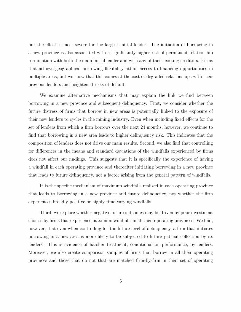
An illustration of the identification strategy is provided in Figure 2. As described in

the figure, we are contrasting two firms with headquarters in the same province (which

is Lima in this example). Both firms have a operating province in which they do not

currently borrow (Anta for Firm 1 and Puno for Firm 2). Firm 1 experiences a maximum

monthly windfall in each of its operating provinces, while Firm 2 does not. The first-stage

(equation (2)) prediction is that Firm 1 will initiate borrowing in a new province (Anta),

while Firm 2 will not initiate borrowing in a new province (Puno). In the second stage

(equation (3)), we explore the implications of the initiation of borrowing in a new province

by contrasting delinquency outcomes for Firms 1 and 2. Although it is not illustrated in

Figure 2, our approach also controls for both the maximum and average windfalls in all of a

firm’s borrowing provinces and firm fixed effects.

The exclusion restriction for this proposed instrument requires that delinquency

outcomes for Firms 1 and 2 be unrelated to their cross-province patterns of maximum

22

monthly windfalls other than through the mechanism of the initiation of borrowing in a

new province. From the standpoint of general plausibility, given that we are controlling

for the overall maximum windfall and the average windfall across all borrowing provinces

(and firm and headquarter province-year-month fixed effects), there is not a clear reason

why experiencing a maximum shock in each operating province should have a direct effect

on firm performance; we are already controlling for the largest and average shocks. In

other words, given that Firms 1 and 2 have the same maximum and average windfalls,

the exclusion restriction requires that their delinquency patterns should differ only due to

Firm 1’s likely initiation of borrowing in a new province. We provide more evidence on

this question in Section 3.7.2 below, in our analysis of firms that already borrow in all their

operating provinces.

As a preliminary matter, we consider whether firms display different financing

characteristics just before periods in which they experience a windfall maximum in all their

operating provinces. That is, we analyze whether firms exhibit shifts in their financial

conditions just prior to being affected by the proposed instrument. We consider some key

financial variables: the fraction of the firm’s debt that has entered judicial status,4 the

fraction of the firm’s debt that is troubled, the delinquency classification of the firm’s loans,5

and the firm’s overall debt balance.

The analysis of firm-demeaned 12-month lagged averages of these financial variables is

provided in Panel I of Table 8. (We consider firm-demeaned variables in light of our inclusion

of firm fixed effects in equations (2) and (3).) We find that the fraction of judicial debt, the

fraction of troubled debt and the debt balances are not statistically different between firms

that experienced a maximum windfall in all their operating provinces over the last twelve

months and those that did not. Firms that experienced a windfall in all their operating

4Judicial status debt is subject to collection through the legal system.5Each borrower in Peru is assigned a classification score by its lender from zero to four based on its

delinquency status: borrowers with current loans are given a score of zero, while borrowers with written-offloans are assigned a score of four. Greater delinquency is thus associated with higher scores. We calculatea weighted average loan classification by weighting by loan balances across different lenders.

23

provinces did have higher weighted classifications (t-statistic=1.65), but the magnitude of

the difference is 0.002, which is very small relative to the classification scale of zero to four and

the mean classification of 0.55. These results suggests that the pre-existing characteristics

of firms affected by the proposed instrument are quite similar to those that were unaffected,

which allays concerns that unobserved variables may influence both the instrument and the

future delinquency outcomes we study.

We test for the instrument first stage (equation (2)) by regressing the indicator for

initiating borrowing in a new province on an indicator for whether the firm experienced

maximum windfalls in each of its operating provinces, and including controls for the level of

the maximum windfall in its borrowing provinces over the last year and the average windfall

across all a firm’s borrowing provinces. We also include firm fixed effects and province-year-

month fixed effects for the firm’s headquarters province to control for firm and local demand

shocks. We show in Panel II of Table 8 that the coefficient on the indicator for experiencing

a maximum windfall in all operating provinces is positive and significant (coefficient=0.023

and t-statistic=5.27). It is indeed the case that having maximum windfalls in each operating

province leads to borrowing in a new province for this set of firms that did not previously

borrow in all their operating provinces.

The result in Panel II of Table 8 shows that the instrument of maximum windfalls

experienced in each operating province leads to the initiation of borrowing in a new province

in the subsequent year. For our second stage analysis (equation (3)), we consider the impact

of this borrowing in a new area on loan delinquency. It would likely require some time for

the initiation of borrowing to have an effect on delinquency. We therefore analyze over the

subsequent 24-month period a firm’s change in weighted classification and an indicator for

whether the firm has a loan that enters judicial status.

Using the two-stage least squares approach detailed above, we regress the change in a

firm’s weighted loan classification on an (instrumented) indicator for initiating borrowing in

a new province and the previously described set of controls. As displayed in the first column

24

of Panel I of Table 9, we find that firms that initiate borrowing in a new province experience

a significant increase (coefficient=1.38 and t-statistic=6.13) in their average weighted loan

classification. That is, these firms become significantly more delinquent.

To provide a sense of the magnitude and importance of the 1.38 increase in

weighted classification, we provide some summary statistics in Table A.2 in the Appendix.

The standard deviation of the weighted classification is 1.26, and the average weighted

classification ranges from 0.35 in the sample year with the highest GDP growth to 0.82 in

the year with the lowest GDP growth. An increase of 1.38 is thus quite large in magnitude. In

a descriptive regression in Table A.2, we show that firms with higher weighted classifications

are much less likely receive new loans over the subsequent 12 months.

We also regress an indicator for having a loan enter judicial status in the subsequent

two years on an (instrumented) indicator for initiating borrowing in a new province and

the previous controls, and we find a positive and significant effect (coefficient=0.28 and t-

statistic=2.81), as shown in the second column of Panel I of Table 9. We provide some

context on the magnitude of this effect in Table A.2 in the Appendix; we show that judicial

status ranges from 0.06 in the highest GDP growth year to 0.15 in the lowest GDP growth

year and that firms in judicial status are substantially less likely to receive new loans.

We have shown that initiating banking in a new province leads to a higher probability of

delinquency; this effect may arise from a financing mechanism, such as a hardening of existing

lender attitudes and a refusal on their part to supply necessary credit, or from an investment

mechanism, such as poorer project choices by the firm. Either of these mechanisms could

lead to the firm not making payments on time. Forcing a delinquent loan into judicial status,

however, is a decision made by lenders, not by the firm. To provide evidence distinguishing

the roles of the financing and investment mechanisms, we consider the impact of initiating

banking in a new province on entry into judicial collection, controlling for the change in

the average weighted classification of a firm’s loans (i.e., the dependent variable from the

regression described in the first column of the panel).

25

We find, as shown in the third column of Panel I of Table 9, that initiating borrowing

in a new region leads to an increase in the probability of entry into judicial status even

when controlling for the change in the weighted classification. We acknowledge that a

regression such as this one that includes a dependent outcome as an explanatory variable

must be interpreted with caution. Nonetheless, keeping this caveat in mind, we argue that

the result provides evidence of the importance of the financing mechanism, as it indicates

that after the firm initiates borrowing in a new province, lenders’ treatment of the firm’s

delinquent debts is tougher: for a given change in loan delinquency, lenders are more likely to

demand judicial collection. Delinquency may be driven by either the investment or financing

mechanisms. The higher probability of transition into judicial status, controlling for changes

in delinquency, however, clearly displays the importance of the financing mechanism.

Overall, the results on debt classifications and entry into judicial status indicate that

when firms initiate borrowing in new provinces for exogenous reasons, they tend to experience

worsened performance of their loans. Financial flexibility, which, from a positive perspective,

offers access to increased borrowing at cheaper rates in more markets, also comes at the cost

of a greater risk of serious default.

3.7.2 Firms that currently borrow in all their operating provinces: falsification

sample

The analysis above of the causal impact on firm performance of initiating a banking

relationship in a new province requires the validity of the proposed instrument, an indicator

for whether the firm experienced a maximum windfall in each of its operating provinces.

We contended above that, controlling for the maximum shock and the average shock, the

instrument should not plausibly be expected to influence firm performance other than

through its effect on whether a firm initiates borrowing in a province. To provide more

evidence to support this argument, we now turn to a set of firms that currently borrow in

all their operating provinces. According to the rules we used to construct our data set, these

26

firms cannot, by definition, expand their lending to a new province. As a result, whether

these firms experienced a maximum windfall in the past year in all their operating provinces

will have no impact on their set of borrowing provinces.

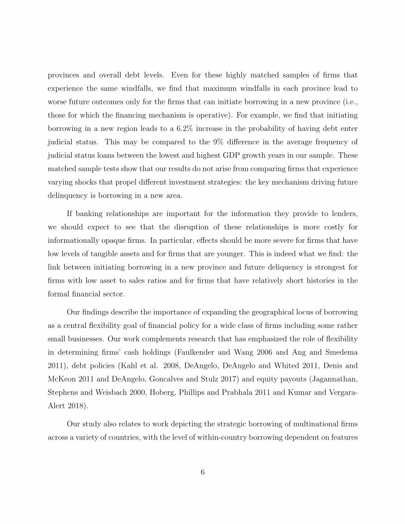
We use this sample of firms to design a falsification test as illustrated in Figure 3.

Firms 3 and 4 in this figure operate in the same provinces as Firms 1 and 2, respectively,

from Figure 2. Firms 3 and 4, however, already borrow in each of their operating provinces,

so mining windfall shocks to their operating provinces cannot lead to initiation of borrowing

in new provinces. As a result, there can be no first stage for these firms. We consider,

however, whether there are any differences in delinquency outcomes for Firms 3 and 4.

Evidence of differential outcomes for these two firms would indicate that the pattern of

maximal windfalls across provinces does have a direct effect on delinquency independent

of its impact on initiating borrowing in a new province; that is, it would suggest that the

exclusion restriction does not hold. Such a result would undermine the causal interpretation

of our two stage design and, in that manner, this specification serves as a falsification test.

For the sample of firms that already borrow in all their operating provinces, we regress

our measures of firm performance on an indicator for whether they experienced a maximum

windfall in all provinces, the maximum windfall across provinces, the average windfall and

firm and time fixed effects. That is, we conduct reduced form regressions of the 2SLS

specifications we described in Section 3.7.1. The results, at leads of two years for both

changes in firm classifications and entry into judicial status, are described in Panel II of

Table 9. We find no significant effect of the indicator for experiencing a maximal windfall

in every province. This supports the argument that experiencing a maximal windfall in

each province has an effect on firm performance only through its influence on the banking

relationships of a firm.

27

3.8 Flexibility and Damaged Relationships- the Financing

Mechanism

The results in Table 9 present the costs of pursuing flexibility; while borrowing in multiple

markets allows firms to exploit local financing supply shocks, it also leads to worse

performance over the subsequent two years. In this section we explore the mechanisms

of this decline in performance.

One potential mechanism is the financing mechanism described above. Firms that

initiate borrowing in new regions may neglect their existing relationships. This neglect

may harm the firm’s ability to manage its debt as new potential lenders will know less

about a firm than its prior banks (Sharpe 1990, Petersen and Rajan 1995 and Dell’Ariccia

2001). Information considerations may therefore restrict a firm’s ability to borrow when it

is dealing with lenders with which it does not have a prior relationship (Petersen and Rajan

1994 and Berger and Udell 1995). Bharath et al. (2011) find that banking relationships lead

to less expensive financing, particularly for borrowers subject to more severe informational

asymmetries, and facilitate the provision of larger loans.

We first consider the impact of initiating borrowing in a new province on the connection

between a firm and its largest lender. Using the same 2SLS specification as in Table 9,

we regress an indicator for whether a firm’s current largest lender (in terms of aggregate

loan size) extends a new loan to the firm in the subsequent two years on an (instrumented)

indicator for whether the firm initiates borrowing in a new province and the previous controls.

We find, as displayed in the first column of Panel I of Table 10, a strong negative effect

(coefficient=-0.73 and t-statistic=-4.25). Initiating borrowing in a new province significantly

reduces a firm’s likelihood of subsequently borrowing from its initial largest lender.

Firms may be expected to have close relationships with their largest lenders. As a

result, a firm’s largest lender is a potential source of emergency funding necessary to refinance

seriously delinquent loans extended by other creditors. It may be argued, therefore, that

28

firms that initiate borrowing in new provinces, and perhaps degrade their relationships with

their largest lenders, may find it more difficult to access the financing required to save

dangerously underperforming loans. A damaged relationship with its largest lender arising

from a firm’s pursuit of geographical financial flexibility may therefore lead to the more

severe delinquency described in Table 9.

Borrowing in new markets can have an impact on a firm’s relationships with other

existing lenders as well. We regress an indicator for whether any of the firm’s initial creditors

extends a new loan in the subsequent two years on an (instrumented) indicator for whether

the firm initiates borrowing in a new province and the standard controls. We find, as

displayed in the second column of Panel I of Table 10, a negative and significant effect

(coefficient=-0.30 and t-statistic=-3.42). Overall, borrowing in new areas leads to a reduced

probability of subsequent financing from existing lenders, and the effect on the largest lender

is especially strong.

It may be argued that perhaps the new financing in a previously unexploited province

simply substitutes for lending from existing creditors for a certain period of time. In other

words, perhaps the firm does not need new loans from its existing creditors for a couple of

years as it is now acquiring financing in a new market. We show, however, in the third column

of Panel I of Table 10 that the causal impact of initiating borrowing in a new province is to

increase the probability (coefficient=0.87 and t-statistic=3.13) that the firm experiences a

permanent termination of its relationship with its initial largest lender (i.e., the firm never

borrows again during our sample period from its initial largest lender). In fact, as shown in

the fourth column of Panel I of Table 10, initiating borrowing in a new province leads to a

significant increase (coefficient=0.73 and t-statistic=3.44) in the log of one plus the number

of terminations in relationships with all initial lenders. Borrowing in a new province does

not lead merely to a temporary disruption in a firm’s relationships with its existing lenders:

it leads to permanent relationship dissolutions.

These results in support of the financing mechanism fit well with those described

29

in earlier sections. In Table 6 we show that higher windfalls in other regions lead to

less borrowing in the focal province, with the effect concentrated on existing borrowing

relationships. In Table 9 we show that maximum windfalls realized across all of a firm’s

operating provinces (and, in particular, realized in operating provinces without any current

financing) make it more likely that a firm will initiate borrowing in a new province. Taken

together, the results in Tables 6 and 9 suggest that high windfalls in current non-borrowing

provinces are associated with both diminished borrowing from existing lenders and increased

borrowing in new areas. The results in Table 10 not only confirm that this is true, but also

establish that the initiation of borrowing in new provinces leads to relationship termination

with previous borrowers, not merely a reduction in the provision of financing.

Even though lenders in a new province may supply financing that had previously been

provided by existing creditors, the delinquency and default results in Panel I of Table 9

make clear that a firm that borrows in new areas does experience worse outcomes. Damaged

relationships with a firm’s current set of lenders cannot easily be replaced due to the

information considerations discussed above.

We are not arguing that borrowing in thriving, previously untapped markets is an error.

Firms, in general, do receive more credit in these markets and average interest rates are lower.

It is useful for firms to be able to borrow in prospering areas. Some firms experience the

good fortune of having already initiated borrowing in markets that later experience positive

windfalls. These firms are able to borrow in successful markets without expanding the

geographical scope of their financing. Other firms are less fortunate and can only receive

loans in flourishing markets by initiating borrowing in new areas. We find that for this

latter group of firms, exercising flexibility by seeking credit in unexploited regions does have

offsetting costs; it results in erosion of the firms’ current set of banking relationships, which

leads to increased risks of severe financial distress.

In order to further examine the plausibility of the financing mechanism, we consider

the same set of future lending outcomes for the sample of firms that currently borrow in all

30

their operating provinces (the sample used for the falsification tests in Section 3.7.2). If the

initiation of new relationships leads to deterioration in future lending outcomes, then these

effects should not be observed for this sample. In Panel II of Table 10 we display results

from the reduced form of our 2SLS specification showing that is indeed true; for firms that

currently borrow in all their operating provinces, achieving a maximum windfall in each

of these provinces has no impact on future lending or relationship terminations with their

current roster of lenders.

3.9 Alternative Mechanisms

We have interpreted the results in Tables 9 and 10 to show that initiating borrowing in a new

province damages existing banking relationships and leads to financial distress through this

financing mechanism. In this section we consider some alternative mechanisms that might

explain the connection between experiencing mining windfalls in all operating provinces and

subsequent distress.

One possibility is that firms that experience windfalls in all their operating provinces

come to borrow from a different set of lenders from firms that do not. For example, it may

be that the former set of firms borrow from banks with exposure to mining areas. Perhaps

subsequent mining busts then lead these lenders to contract their supply of financing thereby

causing harm to their borrowers.

We examine this mechanism by replicating the tests in the top panels of both Tables

9 and 10 while including an additional level of fixed effects: an indicator identifying the full

set of lenders from which a firm borrows over the subsequent 24 months. By including these

fixed effects we are essentially comparing two firms that borrowed from precisely the same

group of lenders over the next two years, one of which previously experienced windfalls in all

of its operating provinces and one of which did not. Given that these firms borrowed from

the same lenders, any differences in subsequent outcomes cannot be attributed to different

characteristics of their lenders.

31

The results are displayed in Panel I of Table 11. We find that in the presence of future

lender fixed effects our instrumented measure of initiating borrowing in a new province

continues to be associated with a worsening debt classification, a higher probability of

entry into judicial status and a disruption of existing borrowing relationships with the firm’s

main initial bank and all initial banks (the one exception is an insignificant impact on the

termination of existing relationships with initial banks). Overall, the evidence is clear that

even controlling for the composition of a firm’s future lenders, initiating borrowing in a new

province leads to worse subsequent delinquent measures.

A second possibility is that future delinquency is driven by the pattern of mining

windfalls in a manner that is unrelated to the initiation of borrowing in a new province. In

Panel II of Table 11 we display results from including fixed effects for the quartiles of both

the average windfall and the standard deviation of the windfall experienced by a firm in

the last 12 months. All the results in Tables 9 and 10 continue to hold in this specification,

suggesting that it is specifically the experience of having a windfall in each operating province

and thereafter initiating borrowing in a new province that leads to future delinquency, not

a factor arising from the general pattern of windfalls.

The instrument and falsification tests depicted in Table 9 provide clear evidence in

support of the argument that the key effect driving default is the initiation of borrowing

in a province. Might it be the case, however, that there are other differences between

firms that borrow in all their operating provinces and those that do not? In Panel I of

Table 12 we show that firms that have some operating provinces without borrowing have

significantly more total firm debt than firms that borrow in all their operating provinces.

Perhaps this difference may drive the differential responses of the two samples of firms to

receiving maximum windfalls in all their provinces. We address this concern by dropping

from consideration the largest loan balance firms that have some provinces with no borrowing

in order to create a sample that has the same mean loan balance as the sample of firms that

borrow in all their operating provinces. As shown in Panel II of Table 12, we replicate

the results of Panel I of Table 9 for this sample of firms with lower loan balances both

32

in specifications in which we include (columns one and two) and exclude (columns three

and four) fixed effects for level of firm debt rounded to the nearest million soles. These

findings indicate that even when adjusting for a firm’s debt level, we continue to find that

experiencing a maximal windfall in each province leads to future delinquency.

As a final test of alternative mechanisms, we create matched samples of firms that

borrow in all their operating provinces and those that do not. For every firm X that borrows

in all of its operating provinces, we identify the group of firms that share precisely the same

operating provinces but that do not borrow in one of those provinces, and we select as a

match the firm from this group that has a debt level that is closest to that of firm X and

that has future delinquency data available. If there is no matching firm, then we exclude

firm X from the sample. We then rerun the tests of Table 9 on these two matched samples.

The firms in these two samples are thus matched precisely in their set of operating provinces

and have similar debt levels. In effect, they are analogous to the firms in Figures 2 and 3 in

which Firms 1 and 3 and Firms 2 and 4 operate in exactly the same provinces.

Under the investment mechanism, the pattern of windfalls across provinces may lead a

firm to make investment choices that lead to bad outcomes. For example, firms may borrow

in boom areas, invest in those areas and then suffer in subsequent busts.6 In this matched

sample test, we are considering firms subject to identical patterns of mining windfalls, some

of which can initiate borrowing in new provinces (the instrument sample) and some of which

cannot (the falsification sample). We show in Panel III of Table 12 that experiencing a

maximum windfall in each province leads to worse delinquency outcomes for firms in the

instrument sample that do not currently borrow in all their operating provinces (and that

can therefore initiate borrowing in a new province). Initiating borrowing in a new province

leads to an 6.2% increase in the probability of entering judicial status, which is similar in

magnitude to the 9% difference between the average rates of judicial status in the lowest

and highest GDP growth years over 2001-2012. A maximum windfall in each province,

however, has no impact on firms in the falsification sample that do currently borrow in all

6We thank an anonymous referee for this point.

33

their operating provinces. These two contrasting sets of findings indicate that our main

results are not likely driven by the effects of windfall patterns on investments, as we are

considering two groups of firms that experience the same windfalls. Only the firms that

initiate borrowing in a new area (i.e., the firms subject to the financing mechanism) exhibit

negative future delinquency outcomes.

3.10 Asset Tangibility and Age

The results in Tables 9 and 10 establish a link between disrupted banking relationships

and future firm financial distress. Replacing ruptured relationships with connections to new

lenders may be difficult due to information asymmetries. These informational issues are

likely to be the most severe for firms with few tangible assets (Harris and Raviv 1991 and

Bester 1985) and for young firms (Petersen and Rajan 1994, Berger and Udell 1995 and

Kysucky and Norden 2015).

We test whether asymmetric information considerations help to drive our results by

conducting two sets of split sample tests. In the first set of tests, we make use of data

from the 2007 economic census to split firms into high- and low-asset-tangibility samples by

comparing their asset-to-sales ratios to the sample median. In Panel I of Table 13 we show

the results from running the tests in the top panels of Tables 9 and 10 separately in the two

samples. We find generally stronger results in the low tangibility sample: the coefficients

are significant and match the expected sign in four of the tests compared to two for the high

tangibility sample; the coefficients are also larger in magnitude in the low tangibility sample.

In the second set of tests we split the sample into new and old firms, where age is

measured by the number of years that the firm has participated in the formal financial

system and the median is used as the dividing point. As shown in Panel II of Table 13, we

find significant results of the expected sign in four of the tests for the sample of new firms,

in contrast to no significant results in the sample of old firms. Overall we find evidence that

the disruption of existing banking relationships is more severe and has a more serious impact

34

on future delinquency for firms with relatively low asset tangibility and for young firms.

Taken together, the results in Table 13 support the argument that the mechanism

linking broken lending relationships to subsequent financial difficulties is mediated through

the effects of asymmetric information. Firms for which information considerations are salient

suffer the greatest costs when they expand their financial flexibility by borrowing in new areas

and, by doing so, weaken their connections to their existing lenders.

4 Conclusion

We examine a group of firms operating in multiple locations in Peru and document that

approximately one quarter of them borrow from banks in different provinces. For these

multiple-province borrowers, only about half of their borrowing occurs in the province where

their headquarters is located. We use variation in commodities prices to estimate the extent

of local mining windfalls in different provinces, and we show that these windfalls generate

finance supply shocks resulting in the provision of more credit at lower average interest rates.

We demonstrate that multi-province firms exploit a geographic real option in financing by

concentrating their borrowing in prospering areas. We find that firms are less likely to expand

their borrowing into new provinces when their current borrowing provinces are enjoying

positive windfalls. We also show that increased geographical financial flexibility comes at

the cost to firms of degrading their existing borrowing relationships. As a result, firms that

begin to borrow in new areas face a heightened risk of financial distress.

Our results highlight both the promise and risks of the pursuit by firms of flexible

access to credit in multiple markets. Financial flexibility is multi-faceted and firm policies

that increase the set of potential borrowing options today may jeopardize future access to

credit in the face of darkening prospects.

35

References

Ang, James and Adam Smedema, 2011, Financial flexibility: Do firms prepare for recession?,

Journal of Corporate Finance 17, 774–787.

Berger, Allen, and Gregory Udell, 1995, Relationship lending and lines of credit in small firm

finance, Journal of Business 68, 351–381.

Bester, Helmut, 1985, Screening vs. rationing in credit markets with imperfect information,

American Economic Review 75: 850–855.

Bharath, Sreedhar T., Sandeep Dahiya, Anthony Saunders, and Anand Srinivasan, 2011,

Lending relationships and loan contract terms, Review of Financial Studies 24, 1141–1203.

Buchuk, David, Borja Larrain, Francisco Munoz, and Francisco Urzua, 2014, The internal

capital markets of business groups: Evidence from intra-group loans, Journal of Financial

Economics 112, 190-212.

Bustos, Paula, Gabriel Garber, and Jacopo Ponticelli, 2016, Capital allocation across regions,

sectors and firms: Evidence from a commodity boom in Brazil, Working Paper, University

of Chicago.

Cole, Rebel, 1998, The importance of relationships to the availability of credit, Journal of

Banking & Finance 22, 959–977.

DeAngelo, Harry, Linda DeAngelo, and Toni M. Whited, 2011, Capital structure dynamics

and transitory debt, Journal of Financial Economics 99, 235–261.

DeAngelo, Harry, Andrei Goncalves, and Rene Stulz, 2017, Corporate Deleveraging and

Financial Flexibility, Review of Financial Studies, forthcoming.

Degryse, Hans and Patrick Van Cayseele, 2000, Relationship lending within a bank-based

system: Evidence from European small business data, Journal of Financial Intermediation

9, 90–109.

36

Dell’Ariccia, Giovanni. 2001, Asymmetric information and the structure of the banking

industry, European Economic Review 45: 1957–1980.

Denis, David, 2011, Financial Flexibility and Corporate Liquidity, Journal of Corporate

Finance 17, 667–674.

Denis, David, and Steve McKeon, 2012, Debt Financing and Financial Flexibility: Evidence

from Pro-Active Leverage Increases, Review of Financial Studies 26, 1897–1929.

Desai, Mihir A., C. Fritz Foley, and James R. Hines, 2004, A multinational perspective on

capital structure choice and internal capital markets, The Journal of Finance 59, 2451-2487.

Detragiache, Enrica, Paolo Garella, and Luigi Guiso, 2000, Multiple versus single banking

relationships: Theory and evidence, The Journal of Finance 55, 1133–1161.

Dou, Yiwei, Stephen G. Ryan, and Youli Zou, 2018, The Effect of Credit Competition on

Banks Loan-Loss Provisions, Journal of Financial and Quantitative Analysis 53: 1195–1226.

Ersahin, Nuri, Rustom M. Irani and Hanh Le, 2016, Creditor Control Rights and Resource

Allocation within Firms, Working Paper, University of Illinois.

Faulkender, Michael and Rong Wang, 2006, Corporate financial policy and the value of cash,

Journal of Finance 61, 1957–1990.

Gamba, Andrea, and Alexander Triantis, 2008, The value of financial flexibility, Journal of

Finance 63, 2263–2296.

Gilje, Erik P., Elena Loutskina, and Philip E. Strahan, 2016, Exporting liquidity: Branch

banking and financial integration, Journal of Finance 71, 1159-1183.

Gopalan, Radhakrishnan, Gregory F. Udell, and Vijay Yerramilli, 2011, Why do firms form

new banking relationships?, Journal of Financial and Quantitative Analysis 46, 1335–1365.

Graham, John, and Campbell Harvey, 2001, The theory and practice of corporate finance:

Evidence from the field, Journal of Financial Economics 60, 187–243.

37

Harris, Milton, and Artur Raviv, 1991, The theory of capital structure, Journal of Finance

46: 297–355.

Hoberg, Gerard, Gordon Phillips, and Nagpurnanand Prabhala, 2014, Product market

threats, payouts, and financial flexibility, Journal of Finance 69, 293–324.

Jagannathan, Murali, Clifford P. Stephens, and Michael Weisbach, 2000, Financial Flexibility

and The Choice Between Dividends and Stock Repurchases, Journal of Financial Economics

57, 355–384.

Kahl, Matthias, Anil Shivdasani, and Yihui Wang, 2008, Do firms use commercial paper to

enhance financial flexibility, Working Paper, University of North Carolina.

Kolasinski, Adam C., 2009, Subsidiary debt, capital structure and internal capital markets,

Journal of Financial Economics 94, 327-343.

Kumar, Anil, and Carles Vergara-Alert, 2018, The Effect of Financial Flexibility on Payout

Policy, Journal of Financial and Quantitative Analysis, forthcoming.

Kysucky, Vlado, and Lars Norden, 2015, The benefits of relationship lending in a cross-

country context: A meta-analysis, Management Science 62: 90–110.

Lamont, Owen, 1997, Cash flow and investment: Evidence from internal capital markets,

Journal of Finance 52, 83-109.

Matsusaka, John G., and Vikram Nanda, 2002, Internal Capital Markets and Corporate

Refocusing, Journal of Financial Intermediation 11, 176-211.

Ozbas, Oguzhan, and David S. Scharfstein, 2010, Evidence on the Dark Side of Internal

Capital Markets, Review of Financial Studies 23, 581-599.

Petersen, Mitchell, and Raghuram Rajan, 1994, The benefits of lending relationships:

Evidence from small business data, Journal of Finance 49, 3–37.

Petersen, Mitchell, and Raghuram G. Rajan, 1995, The effect of credit market competition

38

on lending relationships. Quarterly Journal of Economics 110: 407–443.

Rice, Tara, and Philip E. Strahan, 2010, Does credit competition affect smallfirm finance?

Journal of Finance 65: 861–889.

Samolyk, Katherine, 1994, Banking conditions and regional economic performance: Evidence

of a regional credit channel, Journal of Monetary Economics 34: 259–278.

Sharpe, Steven A. 1990, Asymmetric information, bank lending, and implicit contracts: A

stylized model of customer relationships. Journal of Finance 45: 1069–1087.

Sinnott, Emily, John Nash, and Augusto de la Torre, 2010, Natural resources in Latin

America and the Caribbean - Beyond booms and busts?, The World Bank, Washington D.C.

Stein, Jeremy C., 1997, Internal capital markets and the competition for corporate resources,

The Journal of Finance 52, 111-133.

Xu, Yuqian, Anthony Saunders, Binqing Xiao and Xindan Li, 2017, The Cost of Involuntary

Relationship Destruction, Working Paper, University of Illinois.

39

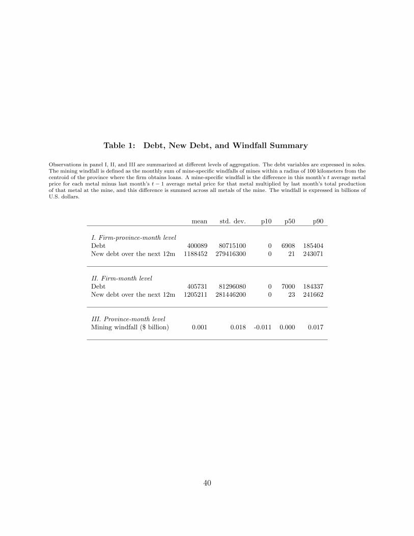
Table 1: Debt, New Debt, and Windfall Summary

Observations in panel I, II, and III are summarized at different levels of aggregation. The debt variables are expressed in soles.The mining windfall is defined as the monthly sum of mine-specific windfalls of mines within a radius of 100 kilometers from thecentroid of the province where the firm obtains loans. A mine-specific windfall is the difference in this month’s t average metalprice for each metal minus last month’s t − 1 average metal price for that metal multiplied by last month’s total productionof that metal at the mine, and this difference is summed across all metals of the mine. The windfall is expressed in billions ofU.S. dollars.

mean std. dev. p10 p50 p90

I. Firm-province-month levelDebt 400089 80715100 0 6908 185404New debt over the next 12m 1188452 279416300 0 21 243071

II. Firm-month levelDebt 405731 81296080 0 7000 184337New debt over the next 12m 1205211 281446200 0 23 241662

III. Province-month levelMining windfall ($ billion) 0.001 0.018 -0.011 0.000 0.017

40

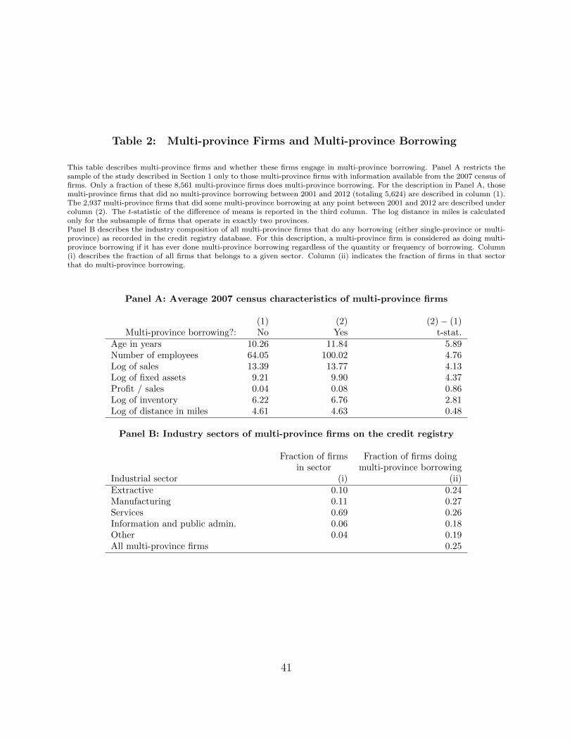
Table 2: Multi-province Firms and Multi-province Borrowing

This table describes multi-province firms and whether these firms engage in multi-province borrowing. Panel A restricts thesample of the study described in Section 1 only to those multi-province firms with information available from the 2007 census offirms. Only a fraction of these 8,561 multi-province firms does multi-province borrowing. For the description in Panel A, thosemulti-province firms that did no multi-province borrowing between 2001 and 2012 (totaling 5,624) are described in column (1).The 2,937 multi-province firms that did some multi-province borrowing at any point between 2001 and 2012 are described undercolumn (2). The t-statistic of the difference of means is reported in the third column. The log distance in miles is calculatedonly for the subsample of firms that operate in exactly two provinces.Panel B describes the industry composition of all multi-province firms that do any borrowing (either single-province or multi-province) as recorded in the credit registry database. For this description, a multi-province firm is considered as doing multi-province borrowing if it has ever done multi-province borrowing regardless of the quantity or frequency of borrowing. Column(i) describes the fraction of all firms that belongs to a given sector. Column (ii) indicates the fraction of firms in that sectorthat do multi-province borrowing.

Panel A: Average 2007 census characteristics of multi-province firms

(1) (2) (2) − (1)Multi-province borrowing?: No Yes t-stat.

Age in years 10.26 11.84 5.89Number of employees 64.05 100.02 4.76Log of sales 13.39 13.77 4.13Log of fixed assets 9.21 9.90 4.37Profit / sales 0.04 0.08 0.86Log of inventory 6.22 6.76 2.81Log of distance in miles 4.61 4.63 0.48

Panel B: Industry sectors of multi-province firms on the credit registry

Fraction of firms Fraction of firms doingin sector multi-province borrowing

Industrial sector (i) (ii)Extractive 0.10 0.24Manufacturing 0.11 0.27Services 0.69 0.26Information and public admin. 0.06 0.18Other 0.04 0.19All multi-province firms 0.25

41

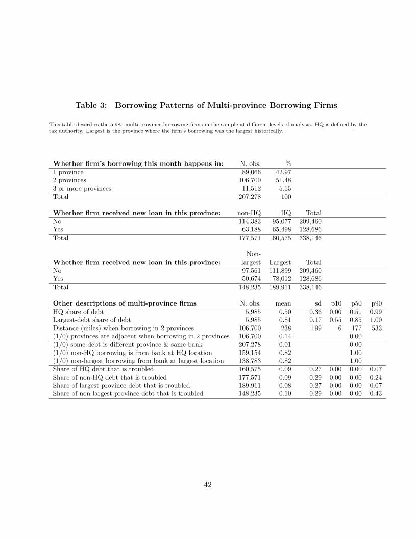
Table 3: Borrowing Patterns of Multi-province Borrowing Firms

This table describes the 5,985 multi-province borrowing firms in the sample at different levels of analysis. HQ is defined by thetax authority. Largest is the province where the firm’s borrowing was the largest historically.

Whether firm’s borrowing this month happens in: N. obs. %1 province 89,066 42.972 provinces 106,700 51.483 or more provinces 11,512 5.55Total 207,278 100

Whether firm received new loan in this province: non-HQ HQ TotalNo 114,383 95,077 209,460Yes 63,188 65,498 128,686Total 177,571 160,575 338,146

Non-Whether firm received new loan in this province: largest Largest TotalNo 97,561 111,899 209,460Yes 50,674 78,012 128,686Total 148,235 189,911 338,146

Other descriptions of multi-province firms N. obs. mean sd p10 p50 p90HQ share of debt 5,985 0.50 0.36 0.00 0.51 0.99Largest-debt share of debt 5,985 0.81 0.17 0.55 0.85 1.00Distance (miles) when borrowing in 2 provinces 106,700 238 199 6 177 533(1/0) provinces are adjacent when borrowing in 2 provinces 106,700 0.14 0.00(1/0) some debt is different-province & same-bank 207,278 0.01 0.00(1/0) non-HQ borrowing is from bank at HQ location 159,154 0.82 1.00(1/0) non-largest borrowing from bank at largest location 138,783 0.82 1.00Share of HQ debt that is troubled 160,575 0.09 0.27 0.00 0.00 0.07Share of non-HQ debt that is troubled 177,571 0.09 0.29 0.00 0.00 0.24Share of largest province debt that is troubled 189,911 0.08 0.27 0.00 0.00 0.07Share of non-largest province debt that is troubled 148,235 0.10 0.29 0.00 0.00 0.43

42

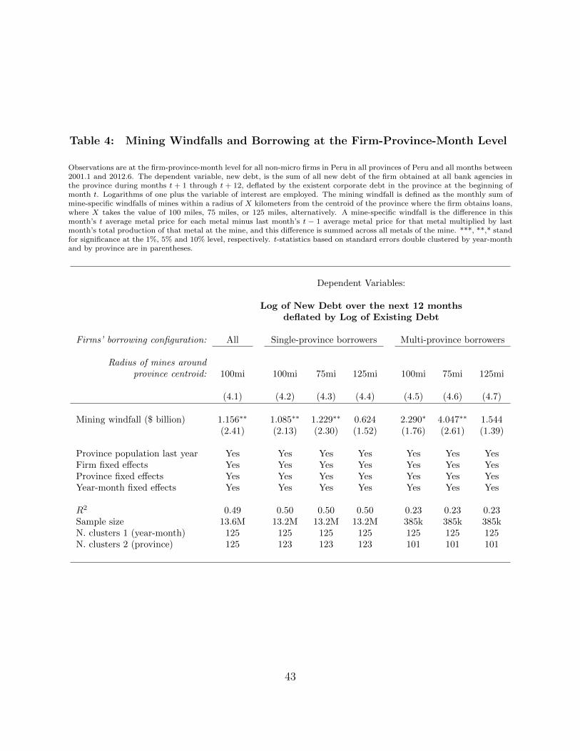
Table 4: Mining Windfalls and Borrowing at the Firm-Province-Month Level

Observations are at the firm-province-month level for all non-micro firms in Peru in all provinces of Peru and all months between2001.1 and 2012.6. The dependent variable, new debt, is the sum of all new debt of the firm obtained at all bank agencies inthe province during months t + 1 through t + 12, deflated by the existent corporate debt in the province at the beginning ofmonth t. Logarithms of one plus the variable of interest are employed. The mining windfall is defined as the monthly sum ofmine-specific windfalls of mines within a radius of X kilometers from the centroid of the province where the firm obtains loans,where X takes the value of 100 miles, 75 miles, or 125 miles, alternatively. A mine-specific windfall is the difference in thismonth’s t average metal price for each metal minus last month’s t − 1 average metal price for that metal multiplied by lastmonth’s total production of that metal at the mine, and this difference is summed across all metals of the mine. ***, **,* standfor significance at the 1%, 5% and 10% level, respectively. t-statistics based on standard errors double clustered by year-monthand by province are in parentheses.

Dependent Variables:

Log of New Debt over the next 12 monthsdeflated by Log of Existing Debt

Firms’ borrowing configuration: All Single-province borrowers Multi-province borrowers

Radius of mines aroundprovince centroid: 100mi 100mi 75mi 125mi 100mi 75mi 125mi

(4.1) (4.2) (4.3) (4.4) (4.5) (4.6) (4.7)

Mining windfall ($ billion) 1.156∗∗ 1.085∗∗ 1.229∗∗ 0.624 2.290∗ 4.047∗∗ 1.544(2.41) (2.13) (2.30) (1.52) (1.76) (2.61) (1.39)

Province population last year Yes Yes Yes Yes Yes Yes YesFirm fixed effects Yes Yes Yes Yes Yes Yes YesProvince fixed effects Yes Yes Yes Yes Yes Yes YesYear-month fixed effects Yes Yes Yes Yes Yes Yes Yes

R2 0.49 0.50 0.50 0.50 0.23 0.23 0.23Sample size 13.6M 13.2M 13.2M 13.2M 385k 385k 385kN. clusters 1 (year-month) 125 125 125 125 125 125 125N. clusters 2 (province) 125 123 123 123 101 101 101

43

Table 5: Mining Windfalls and Commercial Interest Rates

Observations are at the bank-currency-month level. Mining windfalls are averaged over all provinces of the bank each month,using as weights the amount of lending of the branches of the bank in those provinces. Currencies of origination are Soles andU.S. dollars. An interest rate of 20% is expressed as 0.20 for either currency. ***, **,* stand for significance at the 1%, 5% and10% level, respectively. t-statistics based on standard errors clustered by bank are in parentheses.

Dependent Variables:

Commercial Rates on Loans Commercial Rates on Loansof 1 Year or Less Maturity of more than 1 Year Maturity

averaged over the next 12 months averaged over the next 12 months

(5.1) (5.2)

W. Av. mining windfall ($ billion) −0.175∗∗ −0.223∗∗∗

(−2.35) (−2.74)

Currency dummy Yes YesBank fixed effects Yes YesYear-month fixed effects Yes Yes

R2 0.77 0.74Sample size 8020 7812N. clusters (bank) 51 49

44

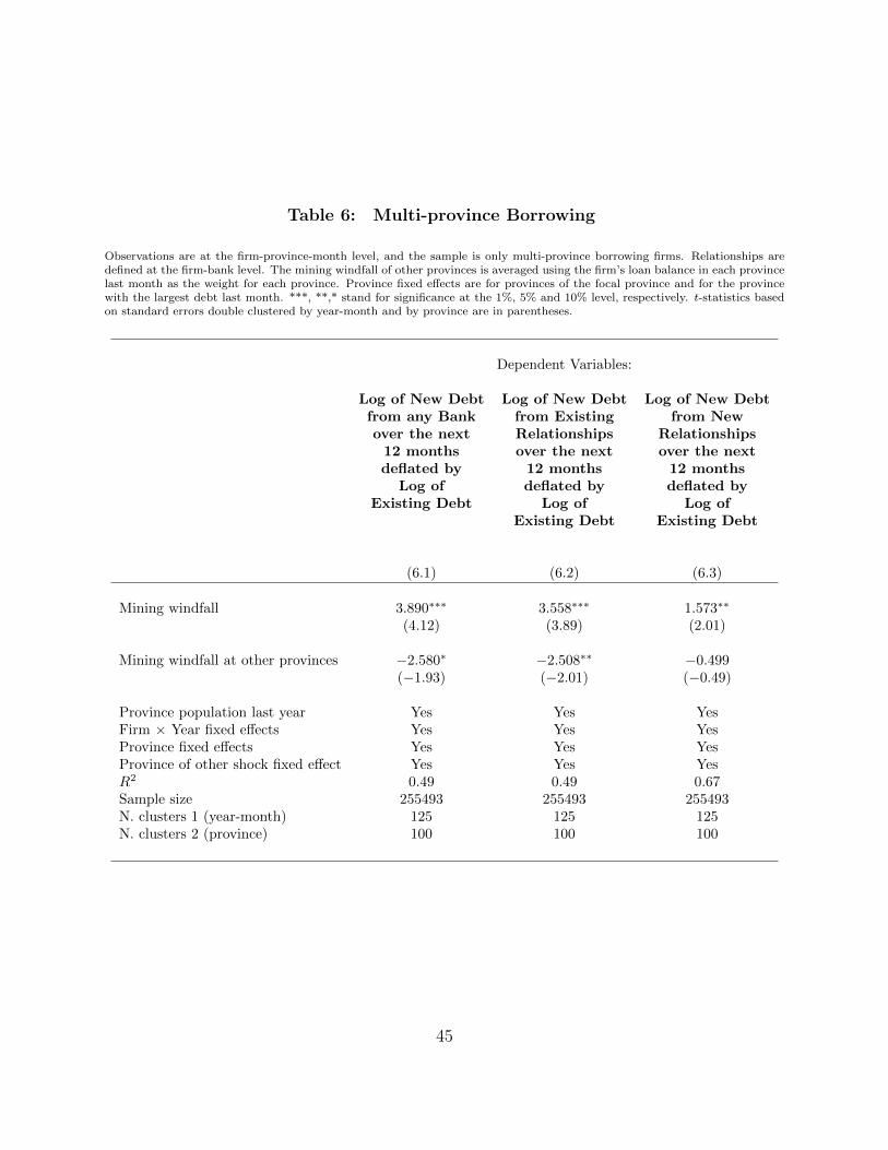
Table 6: Multi-province Borrowing

Observations are at the firm-province-month level, and the sample is only multi-province borrowing firms. Relationships aredefined at the firm-bank level. The mining windfall of other provinces is averaged using the firm’s loan balance in each provincelast month as the weight for each province. Province fixed effects are for provinces of the focal province and for the provincewith the largest debt last month. ***, **,* stand for significance at the 1%, 5% and 10% level, respectively. t-statistics basedon standard errors double clustered by year-month and by province are in parentheses.

Dependent Variables:

Log of New Debt Log of New Debt Log of New Debtfrom any Bank from Existing from Newover the next Relationships Relationships

12 months over the next over the nextdeflated by 12 months 12 months

Log of deflated by deflated byExisting Debt Log of Log of

Existing Debt Existing Debt

(6.1) (6.2) (6.3)

Mining windfall 3.890∗∗∗ 3.558∗∗∗ 1.573∗∗

(4.12) (3.89) (2.01)

Mining windfall at other provinces −2.580∗ −2.508∗∗ −0.499(−1.93) (−2.01) (−0.49)

Province population last year Yes Yes YesFirm × Year fixed effects Yes Yes YesProvince fixed effects Yes Yes YesProvince of other shock fixed effect Yes Yes YesR2 0.49 0.49 0.67Sample size 255493 255493 255493N. clusters 1 (year-month) 125 125 125N. clusters 2 (province) 100 100 100

45

Table 7: Initiating Firms’ Borrowing in an Existing Province

Observations are at the firm-province-month level for all firms operating in multiple provinces, including only those provinceswhere the firm has never borrowed before and where there is a bank present. ***, **,* stand for significance at the 1%, 5% and10% level, respectively. t-statistics based on standard errors double clustered by year-month and by province are in parentheses.

Dependent Variables:

Firm Initiates Borrowing in this Provinceover the next...

12 months month

(7.1) (7.2)

Maximum windfall in all firm’s borrowing provinces −0.039∗∗∗ −0.005∗∗∗

(−3.99) (−2.72)

Firm fixed effects Yes YesProvince-year-month fixed effects Yes YesR2 0.37 0.85Sample size 3.88M 3.88MN. clusters 1 (year-month) 138 138N. clusters 2 (province) 149 149

46

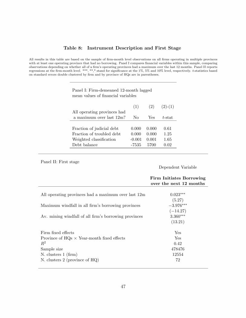
Table 8: Instrument Description and First Stage

All results in this table are based on the sample of firm-month level observations on all firms operating in multiple provinceswith at least one operating province that had no borrowing. Panel I compares financial variables within this sample, comparingobservations depending on whether all of a firm’s operating provinces had a maximum over the last 12 months. Panel II reportsregressions at the firm-month level. ***, **,* stand for significance at the 1%, 5% and 10% level, respectively. t-statistics basedon standard errors double clustered by firm and by province of HQs are in parentheses.

Panel I: Firm-demeaned 12-month laggedmean values of financial variables

(1) (2) (2)-(1)All operating provinces hada maximum over last 12m? No Yes t-stat

Fraction of judicial debt 0.000 0.000 0.61Fraction of troubled debt 0.000 0.000 1.25Weighted classification -0.001 0.001 1.65Debt balance -7535 5700 0.02

Panel II: First stageDependent Variable

Firm Initiates Borrowingover the next 12 months

All operating provinces had a maximum over last 12m 0.023∗∗∗

(5.27)Maximum windfall in all firm’s borrowing provinces −3.976∗∗∗

(−14.27)Av. mining windfall of all firm’s borrowing provinces 3.360∗∗∗

(13.21)

Firm fixed effects YesProvince of HQs × Year-month fixed effects YesR2 0.42Sample size 478476N. clusters 1 (firm) 12554N. clusters 2 (province of HQ) 72

47

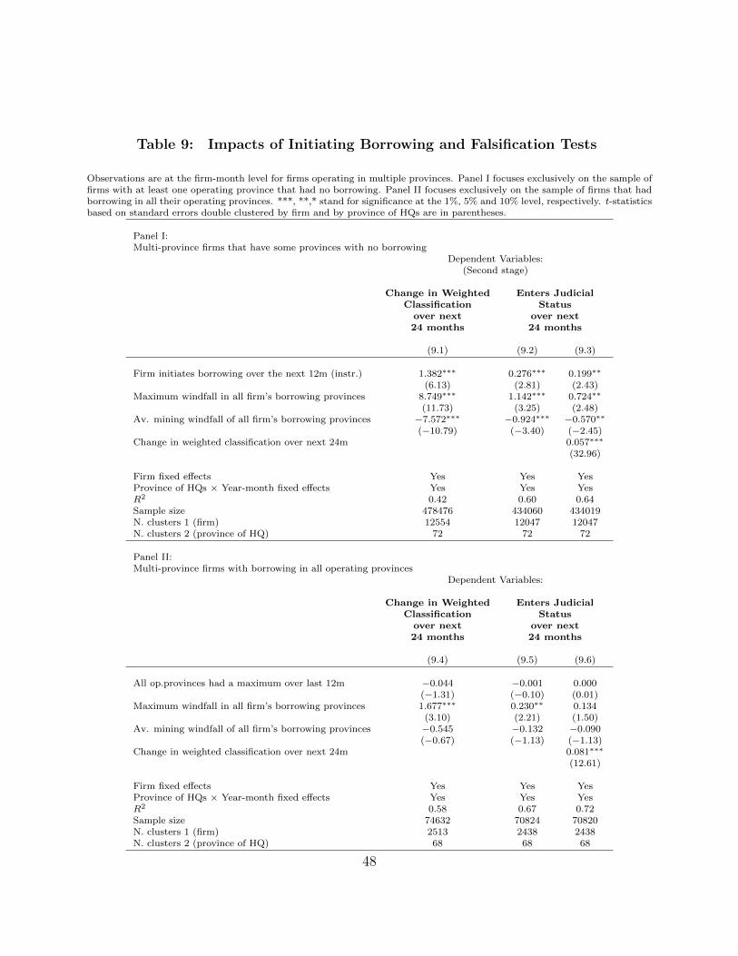
Table 9: Impacts of Initiating Borrowing and Falsification Tests

Observations are at the firm-month level for firms operating in multiple provinces. Panel I focuses exclusively on the sample offirms with at least one operating province that had no borrowing. Panel II focuses exclusively on the sample of firms that hadborrowing in all their operating provinces. ***, **,* stand for significance at the 1%, 5% and 10% level, respectively. t-statisticsbased on standard errors double clustered by firm and by province of HQs are in parentheses.

Panel I:Multi-province firms that have some provinces with no borrowing

Dependent Variables:(Second stage)

Change in Weighted Enters JudicialClassification Status

over next over next24 months 24 months

(9.1) (9.2) (9.3)

Firm initiates borrowing over the next 12m (instr.) 1.382∗∗∗ 0.276∗∗∗ 0.199∗∗

(6.13) (2.81) (2.43)Maximum windfall in all firm’s borrowing provinces 8.749∗∗∗ 1.142∗∗∗ 0.724∗∗

(11.73) (3.25) (2.48)Av. mining windfall of all firm’s borrowing provinces −7.572∗∗∗ −0.924∗∗∗ −0.570∗∗

(−10.79) (−3.40) (−2.45)Change in weighted classification over next 24m 0.057∗∗∗

(32.96)

Firm fixed effects Yes Yes YesProvince of HQs × Year-month fixed effects Yes Yes YesR2 0.42 0.60 0.64Sample size 478476 434060 434019N. clusters 1 (firm) 12554 12047 12047N. clusters 2 (province of HQ) 72 72 72

Panel II:Multi-province firms with borrowing in all operating provinces

Dependent Variables:

Change in Weighted Enters JudicialClassification Status

over next over next24 months 24 months

(9.4) (9.5) (9.6)

All op.provinces had a maximum over last 12m −0.044 −0.001 0.000(−1.31) (−0.10) (0.01)

Maximum windfall in all firm’s borrowing provinces 1.677∗∗∗ 0.230∗∗ 0.134(3.10) (2.21) (1.50)

Av. mining windfall of all firm’s borrowing provinces −0.545 −0.132 −0.090(−0.67) (−1.13) (−1.13)

Change in weighted classification over next 24m 0.081∗∗∗

(12.61)

Firm fixed effects Yes Yes YesProvince of HQs × Year-month fixed effects Yes Yes YesR2 0.58 0.67 0.72Sample size 74632 70824 70820N. clusters 1 (firm) 2513 2438 2438N. clusters 2 (province of HQ) 68 68 68

48

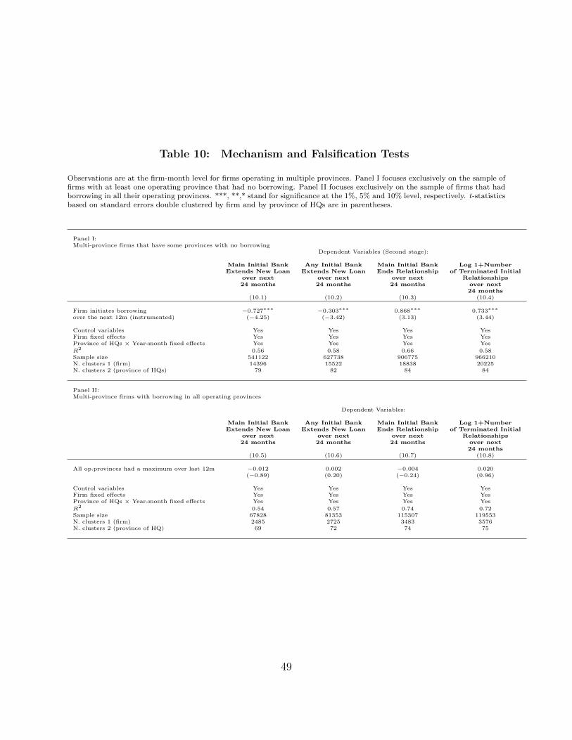
Table 10: Mechanism and Falsification Tests

Observations are at the firm-month level for firms operating in multiple provinces. Panel I focuses exclusively on the sample offirms with at least one operating province that had no borrowing. Panel II focuses exclusively on the sample of firms that hadborrowing in all their operating provinces. ***, **,* stand for significance at the 1%, 5% and 10% level, respectively. t-statisticsbased on standard errors double clustered by firm and by province of HQs are in parentheses.

Panel I:Multi-province firms that have some provinces with no borrowing

Dependent Variables (Second stage):

Main Initial Bank Any Initial Bank Main Initial Bank Log 1+NumberExtends New Loan Extends New Loan Ends Relationship of Terminated Initial

over next over next over next Relationships24 months 24 months 24 months over next

24 months(10.1) (10.2) (10.3) (10.4)

Firm initiates borrowing −0.727∗∗∗ −0.303∗∗∗ 0.868∗∗∗ 0.733∗∗∗

over the next 12m (instrumented) (−4.25) (−3.42) (3.13) (3.44)

Control variables Yes Yes Yes YesFirm fixed effects Yes Yes Yes YesProvince of HQs × Year-month fixed effects Yes Yes Yes Yes

R2 0.56 0.58 0.66 0.58Sample size 541122 627738 906775 966210N. clusters 1 (firm) 14396 15522 18838 20225N. clusters 2 (province of HQs) 79 82 84 84

Panel II:Multi-province firms with borrowing in all operating provinces

Dependent Variables:

Main Initial Bank Any Initial Bank Main Initial Bank Log 1+NumberExtends New Loan Extends New Loan Ends Relationship of Terminated Initial

over next over next over next Relationships24 months 24 months 24 months over next

24 months(10.5) (10.6) (10.7) (10.8)

All op.provinces had a maximum over last 12m −0.012 0.002 −0.004 0.020(−0.89) (0.20) (−0.24) (0.96)

Control variables Yes Yes Yes YesFirm fixed effects Yes Yes Yes YesProvince of HQs × Year-month fixed effects Yes Yes Yes Yes

R2 0.54 0.57 0.74 0.72Sample size 67828 81353 115307 119553N. clusters 1 (firm) 2485 2725 3483 3576N. clusters 2 (province of HQ) 69 72 74 75

49

Table

11:

Outc

om

es

and

Mech

anis

mco

ntr

oll

ing

for

Lender

Com

bin

ati

on

sand

Pri

or

Sh

ock

s

Ob

serv

ati

on

sare

at

the

firm

-month

level

for

all

firm

sop

erati

ng

inm

ult

iple

pro

vin

ces

that

had

at

least

on

eop

erati

ng

pro

vin

ceth

at

had

no

borr

ow

ing.

***,

**,*

stan

dfo

rsi

gn

ifica

nce

at

the

1%

,5%

an

d10%

level

,re

spec

tivel

y.t-

stati

stic

sb

ase

don

stan

dard

erro

rsd

ou

ble

clu

ster

edby

firm

an

dby

pro

vin

ceof

HQ

sare

inp

are

nth

eses

.

Panel

I:Set

of

lenders

over

the

next

24

month

sfi

xed

eff

ects

Dep

endent

Vari

able

s(S

econd

stage):

Change

inW

eig

hted

Enters

Main

Init

ial

Bank

Any

Init

ial

Bank

Main

Init

ial

Bank

Log

1+

Num

ber

Cla

ssifi

catio

nJudic

ial

Extends

New

Loan

Extends

New

Loan

Ends

Rela

tio

nship

of

Term

inated

Init

ial

over

next

over

next

over

next

over

next

over

next

Rela

tio

nship

s24

months

24

months

24

months

24

months

24

months

over

next

24

months

(11.1

)(1

1.2

)(1

1.3

)(1

1.4

)(1

1.5

)(1

1.6

)

Fir

min

itia

tes

borr

ow

ing

1.4

53∗∗∗

0.2

67∗∗

−0.9

69∗

−0.3

72∗∗

0.8

24∗∗

0.3

94

over

the

next

12m

(inst

rum

ente

d)

(4.6

6)

(2.1

3)

(−1.9

3)

(−2.0

6)

(1.9

7)

(1.1

0)

Contr

ol

vari

able

sY

es

Yes

Yes

Yes

Yes

Yes

Fir

mfi

xed

eff

ects

Yes

Yes

Yes

Yes

Yes

Yes

Pro

vin

ce

of

HQ

s×

Year-

month

fixed

eff

ects

Yes

Yes

Yes

Yes

Yes

Yes

Set

of

lenders

next

24m

fixed

eff

ects

Yes

Yes

Yes

Yes

Yes

Yes

R2

0.5

30.7

10.6

30.6

80.7

40.7

4Sam

ple

size

477187

432924

539747

626326

905264

964701

N.

clu

sters

1(fi

rm)

12542

12034

14385

15513

18832

20219

N.

clu

sters

2(p

rovin

ce

of

HQ

)72

72

79

82

84

84

Panel

II:

Inclu

din

gla

st12m

mean

shock

quart

ile

and

standard

devia

tion

shock

quart

ile

fixed

eff

ects

Dep

endent

Vari

able

s(S

econd

stage):

Change

inW

eig

hted

Enters

Main

Init

ial

Bank

Any

Init

ial

Bank

Main

Init

ial

Bank

Log

1+

Num

ber

Cla

ssifi

catio

nJudic

ial

Extends

New

Loan

Extends

New

Loan

Ends

Rela

tio

nship

of

Term

inated

Init

ial

over

next

over

next

over

next

over

next

over

next

Rela

tio

nship

s24

months

24

months

24

months

24

months

24

months

over

next

24

months

(11.7

)(1

1.8

)(1

1.9

)(1

1.1

0)

(11.1

1)

(11.1

2)

Fir

min

itia

tes

borr

ow

ing

1.3

92∗∗∗

0.2

80∗∗

−0.5

95∗∗∗

−0.2

21∗∗

0.8

75∗∗∗

0.6

12∗∗∗

over

the

next

12m

(inst

rum

ente

d)

(5.7

8)

(2.6

9)

(−4.1

9)

(−2.4

8)

(6.2

7)

(5.0

4)

Contr

ol

vari

able

sN

oN

oN

oN

oN

oN

oL

ast

12m

avera

ge

shock

quart

ile

fixed

eff

ects

Yes

Yes

Yes

Yes

Yes

Yes

Last

12m

std.d

ev.

shock

quart

ile

fixed

eff

ects

Yes

Yes

Yes

Yes

Yes

Yes

Fir

mfi

xed

eff

ects

Yes

Yes

Yes

Yes

Yes

Yes

Pro

vin

ce

of

HQ

s×

Year-

month

fixed

eff

ects

Yes

Yes

Yes

Yes

Yes

Yes

R2

0.4

10.6

00.5

40.5

40.6

50.5

7Sam

ple

size

478915

434479

577451

797234

964476

1221138

N.

clu

sters

1(fi

rm)

12564

12058

15630

16578

20478

21521

N.

clu

sters

2(p

rovin

ce

of

HQ

)72

72

80

82

84

85

50

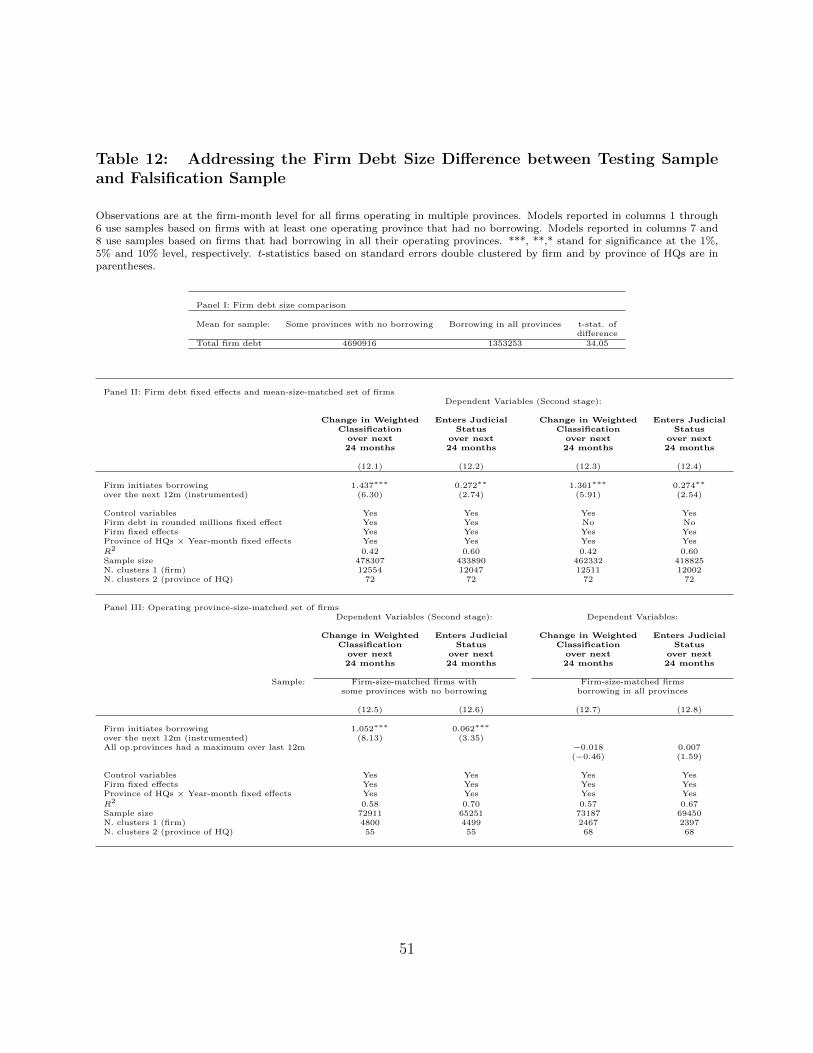
Table 12: Addressing the Firm Debt Size Difference between Testing Sampleand Falsification Sample

Observations are at the firm-month level for all firms operating in multiple provinces. Models reported in columns 1 through6 use samples based on firms with at least one operating province that had no borrowing. Models reported in columns 7 and8 use samples based on firms that had borrowing in all their operating provinces. ***, **,* stand for significance at the 1%,5% and 10% level, respectively. t-statistics based on standard errors double clustered by firm and by province of HQs are inparentheses.

Panel I: Firm debt size comparison

Mean for sample: Some provinces with no borrowing Borrowing in all provinces t-stat. ofdifference

Total firm debt 4690916 1353253 34.05

Panel II: Firm debt fixed effects and mean-size-matched set of firmsDependent Variables (Second stage):

Change in Weighted Enters Judicial Change in Weighted Enters JudicialClassification Status Classification Status

over next over next over next over next24 months 24 months 24 months 24 months

(12.1) (12.2) (12.3) (12.4)

Firm initiates borrowing 1.437∗∗∗ 0.272∗∗ 1.361∗∗∗ 0.274∗∗

over the next 12m (instrumented) (6.30) (2.74) (5.91) (2.54)

Control variables Yes Yes Yes YesFirm debt in rounded millions fixed effect Yes Yes No NoFirm fixed effects Yes Yes Yes YesProvince of HQs × Year-month fixed effects Yes Yes Yes Yes

R2 0.42 0.60 0.42 0.60Sample size 478307 433890 462332 418825N. clusters 1 (firm) 12554 12047 12511 12002N. clusters 2 (province of HQ) 72 72 72 72

Panel III: Operating province-size-matched set of firmsDependent Variables (Second stage): Dependent Variables:

Change in Weighted Enters Judicial Change in Weighted Enters JudicialClassification Status Classification Status

over next over next over next over next24 months 24 months 24 months 24 months

Sample: Firm-size-matched firms with Firm-size-matched firmssome provinces with no borrowing borrowing in all provinces

(12.5) (12.6) (12.7) (12.8)

Firm initiates borrowing 1.052∗∗∗ 0.062∗∗∗

over the next 12m (instrumented) (8.13) (3.35)All op.provinces had a maximum over last 12m −0.018 0.007

(−0.46) (1.59)

Control variables Yes Yes Yes YesFirm fixed effects Yes Yes Yes YesProvince of HQs × Year-month fixed effects Yes Yes Yes Yes

R2 0.58 0.70 0.57 0.67Sample size 72911 65251 73187 69450N. clusters 1 (firm) 4800 4499 2467 2397N. clusters 2 (province of HQ) 55 55 68 68

51

Table

13:

Outc

om

es

and

Mech

anis

ms

by

Ass

et

Tangib

ilit

yand

Age

Ob

serv

ati

on

sare

at

the

firm

-month

level

for

firm

sop

erati

ng

inm

ult

iple

pro

vin

ces

wit

hat

least

on

eop

erati

ng

pro

vin

ceth

at

had

no

borr

ow

ing.

Pan

elI

rest

rict

sth

esa

mp

leto

those

firm

sw

hat

wer

efo

un

din

the

Dec

emb

er2007

cen

sus,

an

dsp

lit

the

sam

ple

into

hig

han

dlo

wta

ngib

ilit

yu

sin

gth

e2007

valu

esof

ass

ets

over

sale

s.P

an

elu

seall

ob

serv

ati

on

sco

mp

ari

ng

old

an

dn

ewfi

rms

usi

ng

age

inth

efi

nan

cial

syst

em.

***,

**,

*st

an

dfo

rsi

gn

ifica

nce

at

the

1%

,5%

an

d10%

level

,re

spec

tivel

y.t-

stati

stic

sb

ase

don

stan

dard

erro

rsd

ou

ble

clu

ster

edby

firm

an

dby

pro

vin

ceof

HQ

sare

inp

are

nth

eses

.

Panel

I:H

igh

vs.

Low

Tangib

ilit

ym

easu

red

as

2007

rati

oof

ass

ets

over

sale

sH

igh

tangib

ilit

yL

ow

tangib

ilit

y

Change

Ent.

Main

I.B

.A

ny

Main

I.B

.L

og

1+

NC

hange

Ent.

Main

I.B

.A

ny

Main

I.B

.L

og

1+

Nw

.Cla

ss.

Judic

.N

ew

Loan

New

Loan

Ends

Term

.I.R

el.

w.C

lass

.Judic

.N

ew

Loan

New

Loan

Ends

Term

.I.R

el.

24m

24m

24m

24m

24m

24m

24m

24m

24m

24m

24m

24m

Fir

min

itia

tes

borr

ow

ing

0.0

76

0.2

55∗∗

−0.6

90∗

−0.2

16

0.1

58

−0.7

74∗

3.3

87∗∗

0.2

95∗

−1.0

64∗∗

−0.8

21∗∗

2.2

04

2.6

78

over

the

next

12m

(inst

r.)

(0.1

7)

(2.4

4)

(−1.7

7)

(−1.1

1)

(0.3

5)

(−1.7

9)

(2.1

0)

(1.7

3)

(−2.3

8)

(−2.2

4)

(1.1

6)

(1.5

7)

Contr

ol

vari

able

sY

es

Yes

Yes

Yes

Yes

Yes

Yes

Yes

Yes

Yes

Yes

Yes

Fir

mfi

xed

eff

ects

Yes

Yes

Yes

Yes

Yes

Yes

Yes

Yes

Yes

Yes

Yes

Yes

Pro

v.H

Qs×

Year-

month

f.e.

Yes

Yes

Yes

Yes

Yes

Yes

Yes

Yes

Yes

Yes

Yes

Yes

R2

0.3

10.4

60.4

20.4

40.6

70.5

90.4

40.5

60.4

40.4

60.7

20.6

3Sam

ple

size

177367

173398

188644

215744

273229

285428

110729

109061

126841

145977

200261

211890

N.

clu

sters

1(fi

rm)

3050

3032

3347

3472

3637

3740

2715

2705

3178

3337

3562

3693

N.

clu

sters

2(p

rov.H

Q)

49

48

59

59

60

60

57

57

63

64

65

66

Panel

II:

Old

vs.

new

firm

-month

obse

rvati

ons

base

don

age

inth

efi

nancia

lsy

stem

Old

New

Change

Ent.

Main

I.B

.A

ny

Main

I.B

.L

og

1+

NC

hange

Ent.

Main

I.B

.A

ny

Main

I.B

.L

og

1+

Nw

.Cla

ss.

Judic

.N

ew

Loan

New

Loan

Ends

Term

.I.R

el.

w.C

lass

.Judic

.N

ew

Loan

New

Loan

Ends

Term

.I.R

el.

24m

24m

24m

24m

24m

24m

24m

24m

24m

24m

24m

24m

Fir

min

itia

tes

borr

ow

ing

−6.2

02

−1.1

81

8.5

55

4.1

49

−1.7

52

5.9

94

0.3

75∗

0.0

73∗∗

−0.0

72

0.0

21

0.5

00∗∗

0.4

93∗∗∗

over

the

next

12m

(inst

r.)

(−0.6

6)

(−0.9

1)

(0.9

1)

(1.0

7)

(−0.9

2)

(1.2

1)

(1.7

7)

(2.0

9)

(−0.9

2)

(0.2

8)

(2.1

2)

(3.9

4)

Contr

ol

vari

able

sY

es

Yes

Yes

Yes

Yes

Yes

Yes

Yes

Yes

Yes

Yes

Yes

Fir

mfi

xed

eff

ects

Yes

Yes

Yes

Yes

Yes

Yes

Yes

Yes

Yes

Yes

Yes

Yes

Pro

v.H

Qs×

Year-

month

f.e.

Yes

Yes

Yes

Yes

Yes

Yes

Yes

Yes

Yes

Yes

Yes

Yes

R2

0.4

70.6

60.6

60.7

20.7

60.6

50.5

30.7

20.6

40.6

50.6

70.6

4Sam

ple

size

200215

179301

231753

261331

438391

459368

277049

253572

308211

365315

466906

505336

N.

clu

sters

1(fi

rm)

6093

5600

7206

7592

10684

11160

11534

11063

13467

14696

17585

19121

N.

clu

sters

2(p

rov.H

Q)

60

59

72

73

77

78

66

66

77

79

81

81

52

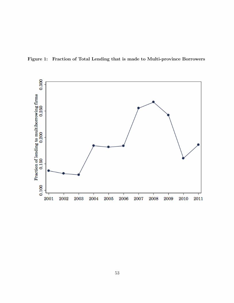
Figure 1: Fraction of Total Lending that is made to Multi-province Borrowers

53

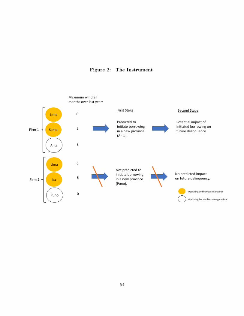
Figure 2: The Instrument

Lima

Maximum windfall months over last year:

Firm 1 Santa

Anta

Lima

Firm 2 Ica

Puno

6

3

3

6

6

0

Predicted to initiate borrowing in a new province (Anta).

Not predicted to initiate borrowing in a new province (Puno).

Potential impact of initiated borrowing on future delinquency.

No predicted impact on future delinquency.

First Stage Second Stage

Operating and borrowing province

Operating but not borrowing province

54

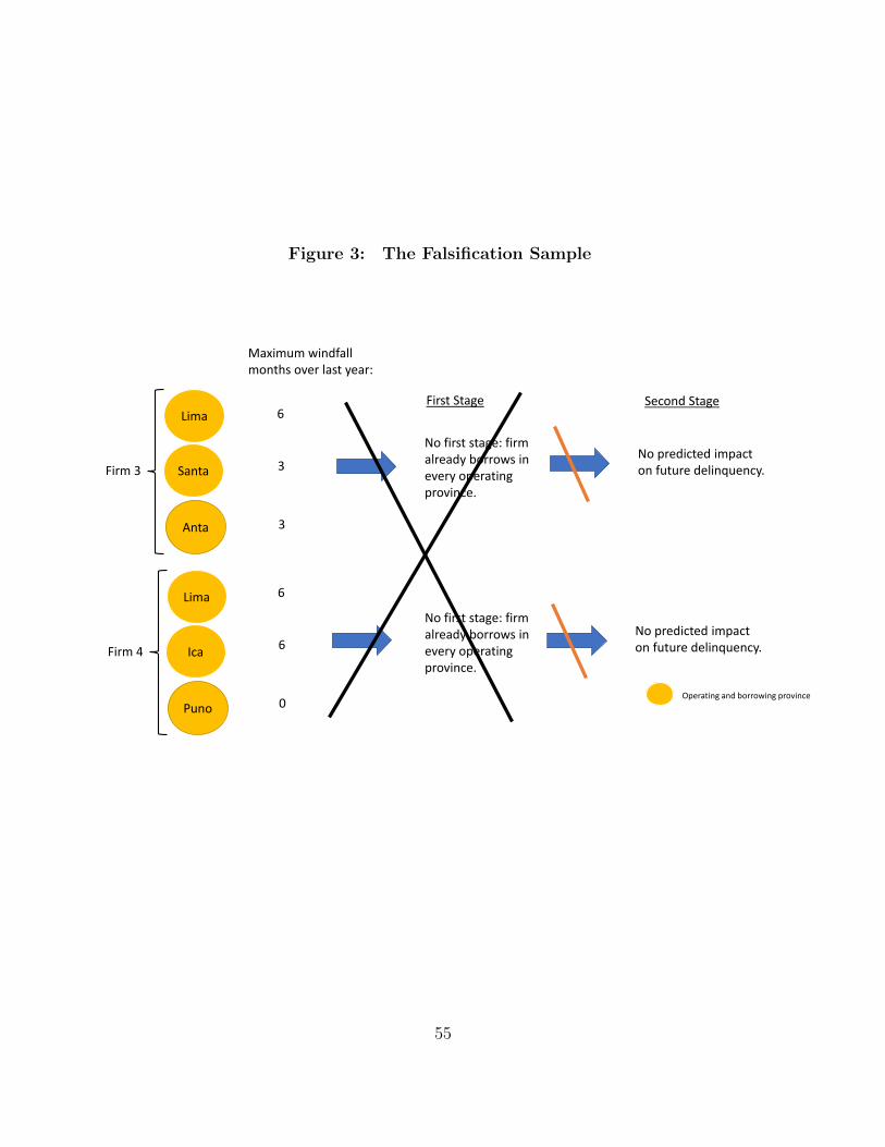
Figure 3: The Falsification Sample

Lima

Maximum windfall months over last year:

Firm 3 Santa

Anta

Lima

Firm 4 Ica

Puno

6

3

3

6

6

0

No first stage: firm already borrows in every operating province.

No predicted impact on future delinquency.

First Stage Second Stage

Operating and borrowing province

No first stage: firm already borrows in every operating province.

No predicted impact on future delinquency.

55

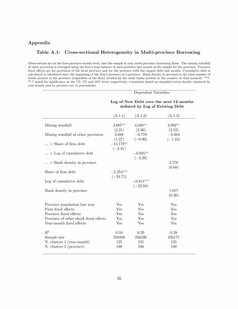
Appendix

Table A.1: Cross-sectional Heterogeneity in Multi-province Borrowing

Observations are at the firm-province-month level, and the sample is only multi-province borrowing firms. The mining windfallof other provinces is averaged using the firm’s loan balance in each province last month as the weight for the province. Provincefixed effects are for provinces of the focal province and for the province with the largest debt last month. Cumulative debt iscalculated is calculated since the beginning of the firm’s presence in a province. Bank density in province is the total number ofbanks present in the province (regardless of the firm) divided by the total banks present in the country at that moment. ***,**,* stand for significance at the 1%, 5% and 10% level, respectively. t-statistics based on standard errors double clustered byyear-month and by province are in parentheses.

Dependent Variables:

Log of New Debt over the next 12 monthsdeflated by Log of Existing Debt

(A.1.1) (A.1.2) (A.1.3)

Mining windfall 3.697∗∗ 4.028∗∗ 3.992∗∗

(2.21) (2.36) (2.52)Mining windfall of other provinces 2.088 −0.719 −3.984

(1.27) (−0.90) (−1.24)... × Share of firm debt −13.178∗∗

(−2.31)... × Log of cumulative debt −0.925∗∗

(−2.29)... × Bank density in province 3.776

(0.68)Share of firm debt −5.254∗∗∗

(−34.71)Log of cumulative debt −0.815∗∗∗

(−22.94)Bank density in province 1.017

(0.36)

Province population last year Yes Yes YesFirm fixed effects Yes Yes YesProvince fixed effects Yes Yes YesProvince of other shock fixed effects Yes Yes YesYear-month fixed effects Yes Yes Yes

R2 0.34 0.29 0.28Sample size 256326 256326 256171N. clusters 1 (year-month) 125 125 125N. clusters 2 (province) 100 100 100

56

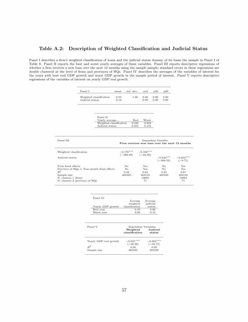
Table A.2: Description of Weighted Classification and Judicial Status

Panel I describes a firm’s weighted classification of loans and the judicial status dummy of its loans the sample in Panel I ofTable 9. Panel II reports the best and worst yearly averages of these variables. Panel III reports descriptive regressions ofwhether a firm receives a new loan over the next 12 months using the sample sample; standard errors in these regressions aredouble clustered at the level of firms and provinces of HQs. Panel IV describes the averages of the variables of interest forthe years with best real GDP growth and worst GDP growth in the sample period of interest. Panel V reports descriptiveregressions of the variables of interest on yearly GDP real growth.

Panel I mean std. dev. p10 p50 p90

Weighted classification 0.55 1.26 0.00 0.00 3.00Judicial status 0.10 0.00 0.00 0.00

Panel IIYearly average... Best WorstWeighted classification 0.345 0.822Judicial status 0.055 0.153

Panel III Dependent Variable:Firm receives new loan over the next 12 months

Weighted classification −0.176∗∗∗ −0.102∗∗∗

(−388.68) (−24.36)Judicial status −0.640∗∗∗ −0.250∗∗∗

(−308.53) (−9.71)

Firm fixed effects No Yes No YesProvince of HQs × Year-month fixed effects No Yes No Yes

R2 0.32 0.62 0.23 0.61Sample size 465225 463118 465239 463133N. clusters 1 (firm) 12003 12004N. clusters 2 (province of HQ) 71 71

Panel IVAverage Average

weighted judicialYearly GDP growth classification statusBest year 0.35 0.06Worst year 0.80 0.15

Panel V Dependent Variables:Weighted Judicial

classification status

Yearly GDP real growth −0.021∗∗∗ −0.004∗∗∗

(−40.06) (−34.17)

R2 0.00 0.00Sample size 465225 465239

57