Embed Size (px)
Citation preview

Financial Feasibility of Maglev Systems in Texas
by
Michael Cline Carla Easton James Gossie
Francisco Parra Edward Penton
Joshua Pickering Anup Shrestha Robert Watson
Parind Oza Amamath Tarikere
Jignesh Thakkar Shekkar Govind
Project Title: Innovative Technologies in Transportation Research Project No. 0-4219 Project Report No. 0-4219-2
Program Coordinator: Mary Owen Project Director: Ron Hagquist
Performed in cooperation with
Texas Department of Transportation Federal Highway Administration
The Department of Civil and Environmental Engineering The University of Texas at Arlington
December 2004

1. Report No. 2. Government Accession No.
FHW AlTX-05/0-4219-2
4. Title and Subtitle Financial Feasibility of Maglev Systems in Texas
7. Author(s)
Michael Cline, Carla Easton, James Gossie, Francisco Parra, Edward Penton, Joshua Pickering, Anup Shrestha, Robert Watson, Parind Oza, Amarnath Tarikere, Jignesh Thakkar, Shekhar Govind 9. Performing Organization Name and Address
Department of Civil and Environmental Engineering The University of Texas at Arlington 416 Yates, 425 Nedderman Hall Arlington, Texas 76019-0308 12. Sponsoring Agency Name and Address
Texas Department of Transportation Research and Technology Implementation Office P. O. Box 5080 Austin, Texas 78763-5080
15. Supplementary Notes
Technical Report Documentation Page 3. Recipient's Catalog No.
5. Report Date
December 2004
6. Performing Organization Code
8. Performing Organization Report No.
10. Work Unit No. (TRAIS)
11. Contract or Grant No.
0-4219
13. Type of Report and Period Covered
Technical Report August 2004
14. Sponsoring Agency Code
Project performed in cooperation with the Texas Department of Transportation and the Federal Highway Administration Project Title: Innovative Technologies in Transportation 16. Abstract
A brief description of different modes possible in the proposed TransTexas Corridor (TTC) is initiated. The main modal alternatives, which include highway, high speed rail, and maglev are discussed in detaiL Alternatives for financing the TTC infrastructure are discussed. A detailed financial feasibility of a maglev system along a hypothetical corridor between DFW and San Antonio is conducted for different cost and ridership assumptions. Conclusions are provided regarding viable financing options for building and operating a maglev system along the TTC.
17. KeyWord
Financial feasibility, TransTexas Corridor, TTC, highway, high speed rail, maglev, financing alternatives
18. Distribution Statement
No restrictions. This document is available to the public through the National Technical Information Service, Springfield, Virginia 22161, www.ntis.gov
19. Security Classif. (of this report)
Unclassified 20. Security Classif. (of this page)
Unclassified 21. No. of Pages 22. Price
119
Form DOT F 1700.7 (8-72) Reproduction of completed page authorized

DISCLAIMER
The contents of this report reflect the views of the authors, who are responsible
for the facts and the accuracy of the data presented herein. The contents do not
necessarily reflect the official views or policies ofthe Federal Highway Administration or
the Texas Department of Transportation. This report does not constitute a standard,
specification, or regulation.
1ll

ACKNOWLEDGEMENTS
This project is being conducted in cooperation with TxDOT and FHW A. The
authors would like to acknowledge Ms. Mary Owen, Program Coordinator (PC), Mr. Ron
Hagquist, Project Director (PD) of the Texas Department of Transportation for their
interest in and support of this project.
December 2004
iv
Michael Cline Carla Easton
James Gossie Francisco Parra Edward Penton
Joshua Pickering Anup Shrestha Robert Watson
ParindOza Am.amath Tarikere
Jignesh Thakkar Shekhar Govind

TABLE OF CONTENTS
Chapter 1 Introduction........ . ....... ............................ .... ......... ................. ............. 1
1.1 Introduction ....... , . ...... ............................ ........ ... .......... .... ............ .... 1
1.2 Problem Statement ....... ..... ......... .............. ......... ................. ......... ...... 2
1.3 Existing Conditions................................. ................................ 2
1.4 Historical Need.. ............................................................................... 4
1.5 Sampling and Measurements.... ........ ... ...... ... ................. .... 6
1.6 Problem Consequences ..................................................................... 11
1.7 Funding.............. ......................................... .............. ........................ 12
1.8 Environmental Impact.... .. .. . . . . .. .... . . . . . . .. . . . . .. . . . . . . . . .. .. . . . . . . .... 14
1.9 Public Opinion.............. ............. .......... .... ......... ................. ......... ....... 18
1.10 Right-of-Way Costs........................................................ 21
1.11 Future Conditions ................................................. '" . . . .. . . 21
1.12 Related Needs............................................................ .... 22
Chapter 2 Description of Alternatives.................................................... 25
2.1 Highway...................................................................... 25
2.2 High Speed Rail. . . .. . ... . .. . . . . .. . . . ... .. . ... . . . ... . .. . . . . . . . . . . . . . .. . . .. . .. 25
2.3 Maglev.... ........... .................. ....... ........... ...... ..... .......... 31
Chapter 3 Analysis of Alternatives....... ....................... ............................ 47
3.1 Highway....................................................................... 47
3.2 High Speed Rail. .. .. . . . . . . . .. . . . . .. . .. .... . . .. . .. . . .. ...... ... . . . ... ... . .. . .. 49
3.3 Maglev.... ..... ...... ... ... ........ .... ... .......... .......... ....... ......... 52
v

3.4 Intangible Benefits............................................................ 57
3.5 Implementation Risks....................... ............................... . 60
Chapter 4 Survey of Financing Alternatives.. . .. . . . . . . . . . . . . . .. . . .. . .. . .. . . . . . . .. . ... . .. 65
4.1 Potential Funding Sources for Capital Costs.............................. 65
4.2 Potential Financing Sources for Capital Costs............................ 67
4.3 Potential Revenue Sources for Operating Costs... ... . . . . . . . .. . .. . .... .... 70
4.4 Public Private Partnership (Alameda Corridor)........................... 71
Chapter 5 Financial Feasibility Analysis ................................................................. 75
5.1 Selection of Route..... ......................................................................... 75
5.2 Scenarios for Financial Analysis............ ......................... ...... 76
5.3 Ridership Assumptions. .. .. .. .... ... .... ... . .. . .. .. .. .. ...... ... .. ... .. ..... 77
5.4 Financial Analysis............................................................ 79
5.5 Discussion of Results. ....... ...................... ............. .............. 91
Chapter 6 Conclusion..... . . . . . . . .. . .. . .. . . . . . . . . . . .. . .. . . . . .. . .. . .. . . .. . .. ... ... ... ...... . . 99
Appendix
A. Abbreviations. . . . ..... . .. . .. . .. . .. . ... ... .. . . . . .. . . . . . .. . . . ... . .. . .. . .. . . .. . . . .. . .. 103
B. Ridership Projections for Texas................................................. 107
C. Cost of Maglev Infrastructure.............. .............. ..... ............... .... 111
Bibliography. .. . .... . . . . . . . . . . . . . . .. . .. . . . . . . . . .. .. . .. . ... . . . . . . .. . . .. . .. ... ... ... . .. . . . . .. ..... 117
Vl

LIST OF FIGURES
Figure No. Page
Figure 1.1 Texas-Mexico border crossing in both directions. NAFTA rail traffic data was provided by railroad companies areas flow characteristics 7
Figure 1.2 Current Amtrak rail lines in Texas and adjoining states traffic and direction design hourly volume 5
Figure 1.3 Projected trips with the study area to CBD by HSR 11
Figure 1.4 Noise levels for various technologies 16 Figure 1.5 Comparison of ambient magnetic field strength between a
Maglev train and common household items 20 Figure 1.6 Annual VMT (Trillions) 22 Figure 1.7 Conceptual ingress and egress to cities along the TTC 24
Figure 2.1 High speed rail projects in America 26 Figure 2.2 Cross section of double track railway alignment 30 Figure 2.3 Modern slab track system, showing the pre-construction
track which is suspended in the structure while concrete is poured around it 31
Figure 2.4 Elevated and at-grade guideway design 41 Figure 2.5 Guideway bendig switches 42 Figure 2.6 Vehic1e undercarriage components 43
Figure 3.1 Maintenance costs for IH-35 49
Figure 5.1 Estimated ridership for 30-minute headway 78 Figure 5.2 Estimated ridership for 20-minute headway 79 Figure 5.3 Payback scenario for headway of 30 minutes with costs
derived from the Baltimore-Washington Maglev project 85 Figure 5.4 Payback scenario for headway of 20 minutes with costs
derived form the Baltimore-Washington Maglev project 87 Figure 5.5 Payback scenario for headway of30 minutes for the Texas
Maglev project 89 Figure 5.6 Payback scenario for headway of 20 minutes for the Texas
Maglev project 91 Figure 5.7 Sensitivity of effective interest rate for headway of 30 minutes
for the Texas Maglev project 93 Figure 5.8 Sensitivity of effective interest rate for headway with 20
minutes for the Texas Maglev project 94
Vll

LIST OF TABLES
Table No. Page
Table 1.1 Conceptual definition of LOS is based on observation of flow characteristics 7
Table 1.2 Projected traffic volumes for IH-35 annual average daily traffic and direction design hourly volume 9
Table 1.3 Travel time in minutes from central business district (CBD) to CBDby HSR 10
Table 1.4 Flights and total passengers leaving from each city 11 Table 1.5 Revenue for proposed corridor by shipping with the brute system 14
Table 2.1 HSR projects around the world 27 Table 2.2 Capital costs for Tri-State II project 27 Table 2.3 O&M costs for the Tri-State II project 28 Table 2.4 Capital costs for the BW Maglev project (all cost in millions) 34 Table 2.5 Operating costs for the BW Maglev project (all costs in millions) 35 Table 2.6 Maintenance costs for the BW Maglev project (all costs in millions) 35 Table 2.7 Energy costs for the BW Maglev project (all costs in millions) 36 Table 2.8 Capital costs for Texas Maglev project (all costs in millions) 37 Table 2.9 O&M costs for the Texas Maglev project (all cost in millions) 38 Table 2.10 Transrapid trainset dimensions 39 Table 2.11 Dimensions for different sizes of the Transrapid trainset 40
Table 3.1 Capital costs escalated to year 2010 54 Table 3.2 Estimated O&M costs for the year 2020 56 Table 3.3 Overall maintenance costs for the year 2020 56
Table 5.1 Annual revenue requirements for 30-minute headway using cost estimate from the Baltimore-Washington Maglev project 83
Table 5.2 Different funding scenarios for varying ridership estimates for 30-minute headway using cost estimate from the Baltimore-Washington Maglev project 84
Table 5.3 Annual revenue requirements for 20-minute headway using cost estimate from the Baltimore-Washington Maglev project 86
Table 5.4 Different funding scenarios for varying ridership estimates for 20-minute headway using cost estimates from the Baltimore-Washington Maglev project 86
Table 5.5 Annual revenue requirements for 30-minute headway for the Texas Maglev project 88
Table 5.6 Different funding scenarios for varying ridership estimates for 30-minute headway for the Texas Maglev project 88
Table 5.7 Annual revenue requirements for 20-minute headway for the Texas Maglev project 90
Vlll

Table 5.8 Different funding scenarios for varying ridership estimates for 20-minute headway for the Texas Maglev project 90
Table 5.9 Average daily gasoline sales in Texas 95 Table 5.10 Gasoline tax increase with Baltimore-Washington costs 96 Table 5.11 Gasoline tax increase with Texas Maglev costs 97
Table B.I Ridership forecast for High Speed Rail in 2020 110
Table C.I Cost estimate for Texas Maglev for 30-minute derived from Baltimore-Washington costs 113
Table C.2 Cost estimate for Texas Maglev for 20-minute headway derived from Baltimore-Washington costs 114
Table C.3 Cost estimate for Texas Maglev for 30-minute headway derived from local costs for construction in Texas 115
Table C.4 Cost estimate for Texas Maglev for 20-minute headway derived from local costs for construction in Texas 116
IX

!!!!!!!!!!!!!!!!!!!"#$%!&'()!*)&+',)%!'-!$-.)-.$/-'++0!1+'-2!&'()!$-!.#)!/*$($-'+3!
44!5"6!7$1*'*0!8$($.$9'.$/-!")':!

CHAPTER 1
INTRODUCTION
1.1 Introduction
In January of 2002, Texas Governor Rick Perry announced an aggressive plan to
modernize the transportation infrastructure in the state of Texas. According to Governor
Perry, "There are four critical transportation problems in Texas: traffic congestion on
every major highway, hazardous material moving across our busiest highways and
through the middle of our urban areas, air pollution in our industrial centers, and
reduced economic activity because of the transportation obstacles businesses face." The
project, dubbed the Trans Texas Corridor (TTC), is an innovative approach to
transportation in a predominantly rural state.
TxDOT has been charged to find a feasible solution to this complicated task
with these criteria:
• Capital, operating, and maintenance costs
• Revenues from the passenger and freight transportation
• Limited access ROW 1,000 to 1,200-feet long
• Separate truck and auto lanes
• High-speed alternative mode of travel for both passengers and freight
• Means of underground utility conveyance such as water pipelines,
fiber optic communications lines, and high-voltage electric lines
This portion of the study will focus on the feasibility and evaluation of the
passenger and freight traffic within the right-of-way (ROW) of the TTC, using
primarily economic factors versus the benefits of each mode to relieve the growing
congestion on the current IH-35 corridor from the DallaslFort Worth area to Laredo,
Texas. The actual length of the corridor has not yet been finalized; therefore the
approximate used for this study is 400 miles. Access to the TTC will be limited to
prevent extended sprawl along its reach. Cost and exact path of the ROWand the
I

underground utilities are not considered in the scope of this report. The research for this
report takes place in the planning stages of the TTC.
1.2 Problem Statement
The existing conditions and the historical background of past attempts to
interconnect the state's major urban areas must be taken into consideration to avoid
making the same mistakes. Measurements of the infrastructure including interstate
corridors, rail corridors, and airways must be acquired to adequately represent current
use of the state network and estimate the future needs of the population. Public opinion
must ultimately be considered for the survival of the project.
1.3 Existing Conditions
Texas metropolitan areas generally utilize rail freight more than other
metropolitan areas. Houston has by far the highest share of rail freight tonnage and per
capita tonnage of the top ten U.S metropolitan areas. Dallas-Fort Worth ranks third in
rail tonnage per capita and fourth in rail tonnage market share. San Antonio also has a
much higher-than-average dependence on rail freight.
Overall the state has a small amount of passenger rail which is served by
Amtrak's Texas Eagle. Amtrak reported 246,414 riders in 2000, which was higher than
in the last 10 years. The Texas Eagle runs from Chicago to San Antonio each day. The
train stops at these major cities: Dallas, Fort Worth, Austin and San Antonio. The train
has a travel time of 15 hours between Texarkana and San Antonio. Once in San
Antonio, the train joins the Transcontinental Sunset Limited, which travels to Los
Angeles, CA. [ Cambridge]
Distances between major urban areas in Texas are generally too long for the
average drive and very short for commuter flights. In general the mode shifts occur at
distances of 150 and 300 miles from auto to rail and from rail to airline respectively.
This is the approximate distance between major urban areas in the state. Increased
airport security has increased boarding time, and thus the resulting factor has increased
the distance of the rail to airline shift. This added propensity for rail cannot be utilized
in Texas because of the extreme limitation of its rail network.
2

1.3.1 North American Free Trade Agreement
On January 1, 1994 the North American Free Trade Agreement (NAFTA) took
effect. One of the primary objectives of the agreement was to eliminate tariffs between
Canada, Mexico, and the United States on qualifying goods by the year 1998.
Originating goods from Canada and Mexico would be tariff free by 2008. Qualifying
goods are goods that are wholly the growth, product or manufacture of a Generalized
System of Preferences (GSP) designated country. It is likely that both rail and truck
freight volumes will expand at a higher-than-average rate in Texas because of the
comparatively rapid population growth rate. NAFTA also strives to promote fair
competition, increase investment in the territories, protect and enforce intellectual
property rights, and establish a framework for further cooperation between the
countries.
NAFTA related volumes are likely to increase the truck and rail volumes, since
Texas shares more of the Mexican border than any other state and serves as the closest
point of entry for 79% of the markets in Mexico, the United States, and Canada. Rail
border crossings over an eight year period are shown in Figure 1.1.
--
~ tOO
G law
Texas - Mexico Rail Border Crossing
~!e
-EaglolP_
-Latlldo -TctOlll
NAFTA
~
1991
· · ·
~§
· : ; : · !
19!N
Year
..",.--
/ / ~
-"
.,.--
1997 1998
Figure 1.1: Texas-Mexico border crossing in both directions. NAFTA rail traffic data was provided by railroad companies serving areas
3

1.4 Historical Need
The state of Texas has made efforts to interconnect major cities; some were
more successful than others. Amtrak and the Texas Triangle were two of the largest,
excluding the original interstate system which was largely a federal effort.
1.4.1 Amtrak
Amtrak started service on May 1, 1971, in New York Penn Station. At that time
Amtrak took over most of the passenger rail operations in the United States except for
three. At this time, Amtrak is the only railroad that has passenger service in the USA.
Presently, Amtrak serves 500 stations and operates in 46 states. Amtrak owns
3% of the tracks that it operates on. The other tracks are owned by freight railroads. On
weekdays, Amtrak operates up to 265 trains per day.
Amtrak was created by the US Congress in 1970 to relieve the freight railroads
of passenger operations and to preserve rail passenger service over a national system of
designated routes. Amtrak was to be a for-profit government corporation which was
granted the right of access to the tracks owned by the freight railroads at incremental
cost and with operating priority over freight trains. It has received federal subsidies for
many years and is expected to make a profit but has not since it was formed.
The Amtrak Texas Eagle originates in Chicago and runs through North Texas
including Dallas and Fort Worth. It connects with the Transcontinental Sunset Limited
in San Antonio which also stops in El Paso and Houston.
The Texas Appropriations Committee gave Amtrak a $5.6 million "bridge" loan
in 1997 to keep the Texas Eagle operating in Texas. The loan was made in order for
Amtrak to work on developing its revenue-generating mail and express business.
Amtrak paid back the loan and was expected to improve services in Texas.
However, Amtrak has failed to make a profit and has shown a 12% decrease on
the Eagle in ridership from a year ago. The Texas Eagle makes service on time only
21 % of the time, which is Amtrak's worst on-time performance rate. Amtrak is
requesting $1.2 billion from Congress to keep the failing railroad running through
4

September 2003. Figure 1.2 is a map of the current Amtrak rail lines in Texas
and adjoining states.
Figure 1.2: Current Amtrak rail lines in Texas and adjoining states
1.4.2 The Texas Triangle
Texas' first high speed rail (HSR) system was to connect Dallas, Houston, and
San Antonio and was to be privately financed. The company that won the high-speed
rail contract was the Texas Train it Grande Vitesse (TGV) Corporation. The contract
was awarded in 1991. Texas TGV Corporation spent over two years of competition
against a rival consortium backing the German ICE (Inter-City Express) technology.
The contract would have covered the design, construction, ownership and operation of
the high-speed rail system.
5

The State of Texas refused to allow state money to be allocated for HSR and
instructed Texas TOV Corporation to secure additional funding from the private sector.
The project's price was estimated at $5.6 billion. After many attempts to secure
funding, the Texas High Speed Rail Authority (THSRA) granted a one-year extension
to secure funding before December 31, 1993.
Texas TOV Corporation was able to get the Warburg Bank of London to issue
$200 million in bonds to finance the project. A major drawback to this agreement was
that the investors in Europe expected to be paid back from their investment within a two
year period by Morrison Knudsen Consulting or their investment would be converted
into shares of the Texas TOV Corporation. Morrison Knudsen Consulting made it
known that the company would not guarantee the bonds. Therefore, the financing fell
through, and the project went past the deadline with no money.
The project's overall estimated cost soared to $6.8 billion. As a result of the high
cost and no way to pay for it, representatives of the state decided that the Texas TOV
Corporation had failed to fulfill its August 1994 contract obligations and the 50-year
HSR development contract was withdrawn. By this time, the Texas TOV Corporation
had invested an estimated $40 million.
1.5 Sampling and Measurements
1.5.1 Interstate LOS
The Highway Capacity Manual (HCM) defines the quality of traffic service
provided by specific highway facilities under specific traffic demands by means oflevel
of service (LOS). The LOS characterizes the operating conditions on the facility in
terms of traffic performance measures related to speed and travel time, freedom to
maneuver, traffic interruptions, comfort, and convenience. The levels of service range
from LOS-A, which is the least congested, to LOS-F, which is the most congested and
is depicted in Table 1.1. The specific definitions of LOS differ by facility type. The
HCM presents a more thorough discussion of the level of service concept, also defined
in the TRB.
6

LOS GENERAL OPERATING
CONDITIONS
A Free flow
B Reasonably free flow
C Stable flow
D Approaching unstable flow
E Unstable flow
F Forced or breakdown flow
Table 1.1: Conceptual definition of LOS is based on observation of flow
characteristics
Multilane Highways may be treated similar to freeways if major crossroads are
infrequent, or if many of the crossroads are grade separated, and if adjacent
development is sparse so as to generate little interference. Even on those highways
where such interference is currently only marginal, the designer should consider the
possibility that by the design year the interference may be extensive unless access to the
highway is well managed. In most cases, the designer should assume that extensive
crossroad and business improvements are likely over the design life of the facility.
1.5.2 Interstate Annual Average Daily Traffic
Highway design should be considered based on the traffic volumes and
characteristics to be served. Traffic volumes indicate the need for the improvement and
directly affect the geometric design features, such as number of lanes, widths,
alignments, and grades. Information on traffic volumes serves to establish the loads for
the geometric highway design.
7

The data collected by State or local agencies include traffic volumes for days of
the year and time of the day, as well as the distribution of vehicles by type and weight.
The data also include information on trends from which the designer may estimate the
traffic to be expected in the future. Traffic data for a road or section of road are
generally available or can be obtained from field studies.
The current AADT volume for a highway is determined when continuous traffic
counts are available. When only periodic counts are taken, the AADT volume can be
estimated by adjusting the periodic counts according to such factors as the season,
month, or day of week.
However, the direct use of AADT volume in the geometric design of highways
is not appropriate except for local and collector roads with relatively low volumes
because it does not indicate traffic volume variations occurring during the various
months of the year, days of the week, and hours of the day. The amount by which the
volume of an average day is exceeded on certain days is appreciable and varied. At
typical rural locations, the volume on certain days may be double the AADT. Thus, a
highway designed for the traffic on an average day would be required to carry a volume
greater than the design volume for a considerable portion of the year, and on many days
the volume carried would be much greater than the design volume.
Trucks occupy more roadway space and have a greater effect on highway traffic
operation than do passenger vehicles. Trucks are normally defined as those vehicles
having manufacturer's gross vehicle weight ratings of 9,000 lb or more and having dual
tires on at least one rear axle.
The overall effect on traffic operation as well as on pavement condition of one
truck is often equivalent to several passenger cars. Thus, the larger the proportion of
trucks in a traffic stream, the greater the traffic demand and the greater the highway
capacity needed. For the geometric design of a highway, it is essential to have traffic
data on vehicles in the truck class. Trucks can be modeled as percentages of total traffic
on a given highway.
8

Texas has become the nation's second most populated state and added nearly as
many new residents over the past decade as California. This high growth rate is likely to
continue in the decades to come and therefore projections play an important role.
Projections indicate that Texas will continue to grow at rates well above the
national average. By 2025, Texas is likely to add another 55 percent to its population to
reach more than 32 million. The U.S. Census Bureau expects Texas to grow 60% faster
than the rest nation from 2000 to 2025. AADT Projections used in this study are based
on 3% annual growth, and can be seen in Table 1.2. The table also indicates the
Directional Design Hourly Volume (DDHV) for the current year and the projections for
2020.
CITIES 2000AADT 2000DDHV 2020DDHV
Laredo to SA 24960 1373 2479
SA to Austin 54590 3002 5423
Austin to Hillsboro 44550 2450 4425
Hillsboro to Dallas 26000 1430 2583
Hillsboro to FW - 23000 1265 2285
Table 1.2: Projected traffic volumes for IH-35 - annual average daily traffic and
direction design hourly volumes [TxDOT]
1.5.3 Rail Service
The AADT for freight cars that move from Laredo to DFW is assumed to be 6 to
8 cars per day from raw data for a 4 day period from a Union Pacific daily dispatch for
a typical train. The observed trains moved an average of 65 cars at an average of 68
gross tons per car. The average overall length for a train was 5700 ft.
9

The Table 1.3 describes the typical travel times between cities in the Texas
Triangle for HSR as projected by Charles River Associates, Inc.
FROM/TO AUSTIN nFW HOUSTON SAN ANTONIO
Austin 0 88 74 42
DFW 88 0 101 118
Houston 74 101 0 116
San Antonio 42 118 r 116 0
Table 1.3: Travel time in minutes from central business district (CBn) to CBn by
HSR [CRA]
1.5.4 Airline Traffic
With the addition of HSR in Texas there will be a decrease in air ridership.
Projections on air ridership are needed in order to estimate the amount of riders that will
be diverted to the TTC's Maglev or HSR system.
The Table 1.4 describes air connect trips between DFW Airport and other Texas
cities if HSR was absent. Charles River Associates projected the growth rates using
Federal Aviation Administration (FAA) forecasts: Fiscal Years 1993-2004 and the
assistance of Stanford Rederer, President of Aviation Planning and finance, Inc.
Washington, D.C. Table 1.4 shows the projected flights.
AVERAGE PASSENGERS PER PASSENGERS CITIES
PLANES PER nAY YEAR (2000) PER YEAR(2020)
Laredo 16 70,234 126,850
San Antonio 129 3,647,094 6,587,057
Austin 240 7,000,000 12,642,779
DFWairport 2222 60,687,122 109,607,693
Love field 679 7,077,549 12,782,841
Total 3293 78,481,999 141,747,220
Table 1.4: Flights and total passengers leaving from each city
10

The largest number of diverted travelers to HSR will come from business air
travelers. Overall HSR is expected to divert 25% of all travel between these cities.
Air travel is expected to increase between the TTC cities at 3% per year. The
AADT for this corridor is approximately 3300 planes per day. The corridor is made up
of the following airports: Austin-Bergstrom International, DFW International Airport,
Dallas Love Field Airport, and San Antonio International Airport. Approximately 75
million passengers flew through these airports in 2000. Figure 1.3 depicts the projected
airport trios in the proposed corridor.
'ii
" I :s ! ... .s -I I
1,800
1,600
1,400
1,200
1,000
800
600
400
200
0
1990
Projected Airport Passenger Trips
-DFWwAustin
- DFW-San Antonio -DFW-Waco --------.: ......... =---=--==----
1995 2000
Vear 2005 2010
Figure 1.3: Projected trips with the study area [eRA]
1.6 Problem Consequences
The existing interstate system was designed to carry a finite number of heavy
trucks during its lifespan. The exponential increase in the volume of truck traffic since
the enactment of NAFTA, while economically beneficial to Texas, has accelerated the
deterioration of its highway network. When the actual number of trucks that pass over
the pavement greatly exceeds the number expected, the end result is a shorter lifespan
11

of the roadway. The rehabilitation and replacement of these affected highways are on
the horizon for TxDOT.
Congestion in urban areas increases as a direct result of the bulkier and slow
moving trucks. Many of these trucks carry hazardous materials near densely populated
areas, thus creating the potential for disaster. The size differential between trucks and
automobiles also hinders visibility. The number of trucks entering Texas cannot legally
be curbed, and is increasing much faster than predicted, so the problem will only
compound.
With the existing problems of the interstate system increasing exponentially, a
new system is needed more than ever. Rehabilitation and replacement of the existing
roadways won't solve the problems at hand. Increased capacity, decreased congestion,
higher speeds, and safer driving conditions can only be accomplished by a new system
that can accommodate the needs of the traveling public. Doing nothing at this point is
not an option.
1-7 Funding
A project of this scale will require a variety of sources to draw funding. Several
obvious sources were named by Governor Perry, but inventive sources should also be
reviewed.
1.7.1 Exclusive Development Agreement
The state will make a contract with a group to do all or a portion of the
following: design, construct, operate, maintain, or finance the transportation project.
The state will conduct a needs assessment for the project and will submit a request for
proposals (RFP) from the competing groups on how they will complete the project. The
state will then select the group that best accommodates the RFP.
1.7.2 Toll Equity
Toll equity makes projects more attractive for private investors by sharing toll
revenue and will supplement project funds to help pay for the corridor.
1.7.3 Regional Mobility Authority
12

Regional Mobility Authority creates partnerships with urban areas to finance,
build, operate, and maintain new toll projects, which will complement and support the
corridor.
1.7.4 Texas Mobility Fund
Texas Transportation Commission is allowed to issue bonds to accelerate
construction on major highway projects. Monies raised from these bonds can be used to
finance road construction on state maintained highways, publicly owned toll roads and
other public transportation projects. Funds for the Texas Mobility Fund will be provided
by the state legislature.
1.7.5 Lease
Areas along the corridor may be leased to private companies to provide services
such as fuel, lodging, and restaurants. The property could be leased at a premium rate,
because the proprietors of these establishments would have a local monopoly.
1.7.6 Parcel Services
Tri-State II high-speed feasibility study produced key factors in the over all
make up of the system. Fares, on-board services (OBS), and parcel services each
contribute to the revenue of the system. OBS supply the food and drinks on the train
and is expected to cover the full cost of operations including contractor's profit. Parcel
services include but are not limited to the following: bank clearings, legal documents,
organs, tissues and other bio-medical products, broadcasting and media equipment,
convention materials, production parts, and other time sensitive items.
These packages can be shipped in what is known as a "Brute" at a size of 6 feet
by 6 feet by 3 feet, which holds on average 432 parcels. Price per parcel is $30. There
can be four parcels per cubic foot with 20% capacity. Generally 10% of gross revenue is
reported as profit. [MnDOT] Table 1.5 shows the revenue for the proposed corridor
given 2020 volume.
l3

NUMBER OF PARCELS NUMBER OF PRICE PER REVENUE PER
PER BRUTE RAILCARS PARCEL TRAIN
432 6 $30.00 $77,760.00
Table 1.5: Revenue for proposed corridor by shipping with the brute system
[MnDOT]
1-8 Environmental Impact
The Environmental Protection Agency (EPA) has established the National
Ambient Air Quality Standards (NAAQS) for criteria pollutants under the Clean Air
Act 1990 and establishes an adequate margin of safety to protect the public health.
Tarrant and Dallas counties are the only non-attainment counties that are located
within the study corridor. Both counties are non-attainment due to the high volumes of
ozone. [Parsons] Ozone pollution is a key component of smog and is typically at its
highest levels during the daytime hours and summer months. Ozone is not emitted
directly into the air; instead it is formed by sunlight heating primarily Oxides of
Nitrogen (NOx) and Volatile Organic Compound (VOC) emissions. NOx is produced
almost entirely as a by-product of high-temperature combustion.
Common sources of NOx include automobiles, trucks, and marine vessels,
construction equipment, power generation, industrial processes, and natural gas
furnaces. VOC includes many organic chemicals that vaporize easily, such as those
found in gasoline and solvents. They are emitted from several sources, including
gasoline stations, motor vehicles, airplanes, trains, boats, petroleum storage tanks, and
oil refineries.
The concentration of ozone in the air is determined by the amount of reactants,
in addition to weather and climatic factors. A combination of intense sunlight, warm
temperatures, stagnant high-pressure weather systems, and low wind speeds cause
ozone to accumulate in harmful amounts.
14

1.8.1 Highway
In May 2001, the 77th Texas Legislature established the Texas Emission
Reduction Plan (TERP), which is the latest effort to help reduce air pollution in Texas.
TERP will administer a program of grants and incentives for improving air quality
throughout the state including on the highways. The program may pay incremental costs
on the purchase or lease of "clean" heavy duty vehicles as well as light duty vehicles
that meet stablished emissions levels. Its funds may also be used to support the
repowering of on-road and off-road diesel vehicles with cleaner engines and assist in
establishing infrastructure for qualifying alternative fuels. [TxDOT]
In the future, TxDOT plans to further reduce its own emissions by using hybrid
electric passenger vehicles, dedicated alternative fuel vehicles, ultra low sulfur diesel,
and emerging technologies for off-road equipment. [TxDOT]
1.8.2 High Speed Rail
Three factors that are typically considered when looking at HSR are noise
pollution, air pollution, and energy consumption.
Noise is sound which is considered undesirable for a variety of reasons, but
usually because of intensity levels. The decibel (dB) is the standard unit used to
measure noise, and the A-weighted decibel (dBA) is used to describe the effect of sound
on a human. When looking at HSR the sources of noise are wheel to rail noise,
aerodynamic noise and electrical noise. Wheel noise can be modeled using 30-log
Speed. Aerodynamic noise can be calculated using 60-log Speed. [Regional Science]
Noise pollution from high-speed rail will generally lower property values in
some locations as well as loss of sleep, lower productivity, psychological discomfort
and annoyance for the residents living close to the railway tracks. While it is impossible
to put a price tag on any of these factors, they must be considered when placing a track
near residential areas. [Regional Science]
Since high-speed rail is electrically powered it can be assumed that there is
practically no mobile pollution source. The actual pollution will be reflected in the
increased electrical energy demand by HSR at point pollution sources across the state.
15

Power plants will have to generate more electricity in order to meet this demand.
Trying to figure out which of the 135 electrical power plants will supply the power will
be difficult, since Texas receives power from nuclear, natural gas, coal and lignite, and
water flow. Each power source employed by the electrical plants has very different
environmental impacts, and all are under intense government regulation. [Regional
Science]
1.8.3 Maglev
Similar to HSR, the environmental aspects impacted by Maglev are nOIse
pollution, air pollution, and energy consumption.
All current mass transit trains produce three primary categories of noise: motor,
rolling, and aerodynamic. The first two types of noise are eliminated with the use of a
Maglev train. The Maglev train uses an electric motor which produces no noise
pollution. There is no wheel contact with a rail therefore there is no rolling noise. The
only noise produced by Maglev is aerodynamic noise and is only significant when it
reaches 125 mph and higher speeds. [Parsons] The Transrapid Maglev train peaks at 98
dBA at a distance from the guideway of 82 feet and speed of the train at 270 mph. Even
at a speed of 155 mph the Maglev train is quieter then a typical commuter train passing
at 50 mph. Figure 1.4 compares the A weighted decibel rating of Maglev to other high
speed trains.
Figure 1.4: Noise levels for various technologies
16

All of this noise is produced by the aerodynamic design of the train itself. The
trains themselves create very little noise, less then freeways and airports, even during
the accelerating and braking of the train. 1 Since the train runs on electricity it lacks the
noise produced by an engine, therefore when approaching a town at a moderate speed,
noise produced is barely louder then the normal noise leveL
Maglev is powered by substations connected to the state's electrical power grid.
The substations receive power from a power plant which turns the mobile pollution
sources of cars into a point source. Reducing the number of cars on the road, and
therefore pollution, is a major goal of implementing Maglev technology. [Parsons] The
train also does very little damage to the surrounding environment. The trains are
propelled by electricity, not by burning fuel, and so they emit no harmful pollutants as
they pass. The Maglev train is adaptable to any area that it may pass through, so there is
no need for much of the earthwork or grade crossings that is often needed with
conventional trains. Maglev trains are also more energy efficient, requiring fifty
percent less energy per person than an automobile and seventy percent less than an
airplane.
Critics have questioned the efficiency of Maglevs with respect to noise,
environmental degradation and safety. In answer to these concerns, Maglev trains
produce small amounts of pollution and are one of the safest modes of transportation.
According to the California High-Speed Rail Authority (CHSRA) there is almost no
danger in this respect. Conventional trains are generally regarded as the safest form of
transportation available today and Maglev trains are even safer than traditional trains.
Magnetic levitation technology in Germany is estimated to be seven hundred times safer
then auto travel and twenty times safer than air traveL The original type of support,
propulsion, braking and guidance system, enclosing the vehicle on the guide way all
contribute to the virtual impossibility of ordinary derailment, even in the event of total
power failure. Also since the propulsion system is run from a control center and trains
are isolated on directional lines, collisions between two trains are almost impossible.
I Hanson, California High Speed Rail Authority (CHSRA)
17

1.9 Public Opinion
The public opinion of a mode can make or break a project. Each mode will have
its own intended set of customers to win over.
1.9.1 Highways
To maximize effectiveness of the environmental decision-making process, the
public along with TxDOT and the resource agencies must create new partnerships and
depart from traditional methods of planning, coordination and review. Ecosystem
mitigation and compensation should be important parts of this approach. The public,
TxDOT and resource agencies must look for "win-win" solutions that work toward
fulfilling objectives that benefit the corridor and the environment and strive to avoid or
minimize adverse environmental impacts. Databases, existing inventories and other
sources are used to identify tracts of land suitable for acquisition or conservation. This
will compensate for unavoidable impacts resulting from the corridor, according to
TxDOT. The TTC project will need to promote:
·Protection, conservation and restoration of important natural and cultural
resources.
• Wise management and sound stewardship of natural, biological and cultural
resources, while providing a range of goods and services such as recreation and
transportation.
-Ecologically sustainable development for current and future generations.
Objectives of the ecosystem and cultural resources must:
·Establish collaborative interagency relationships to promote healthy ecosystems
preserve historic refuges, support safe and efficient multi-modal, multi-use
transportation systems and encourage wise economic growth while recognizing
Texas' social and cultural diversity.
·Focus agency programs to establish collaborative approaches that enhance and
protect natural and cultural resources while providing better transportation
options for the public.
18

-Emphasize through public outreach how the successful integration of
ecological, cultural and socio-economic values makes Texas a better place to
live and work.
1.9.2 High Speed Rail
As Texas highways continue to get more congested, HSR will have to be
presented as an alternative to reduce the over crowded roadways and pollution we face
today. However, in order for HSR to receive funding it needs to gain public support in
the state of Texas.
Some reasons why people commute by automobile are: people value their time.
People find it very difficult to wait for a bus compared with waiting in stop and go
traffic. Rapid transit is not viewed as rapid and is not a cost effective alternative.
Typically rail transit averages 22 mph and may only have a top speed of 55 mph. The
public will have to be convinced that HSR will decrease their travel time considerably
for them to switch modes. Both travel time and out of pocket costs weigh the most to
the over all acceptance of the new system. A trip through the proposed corridor of 400
miles gives the passenger two polar options, plane or auto. The current out of pocket
cost runs approximately $92 for a one-way trip by plane. The travel time for a car is
over five hours. With these two factors HSR will need to stress the point that by
traveling on the alternative mode they can arrive much faster than in their car and at a
lower cost then flying. [Slater]
Special interest group, such as DERAIL (Demanding Ethics, Responsibility, and
Accountability in Legislation) lobbied in strong opposition to the Texas TOV project.
The resistance was founded on classical NIMBY (Not In My Back Yard) beliefs. Noise
and infrastructure is believed to drop property values and hurt farming and ranching.
Mitigation is expected in any large scale project involving reclaiming land by the state.
The Texas TOV Environmental Impact Study (EIS) included over 4,000 public
participants and provided a total of 15,000 separate comments at the 39 different public
hearings. This over whelming response shows the need to involve the public and
interest groups in all steps of this project. [Perl]
19

1.9.3 Maglev
The general public knows very little about Maglev or how it works. Their
understanding of it is limited because Maglev is a new technology. The major
difference between Maglev and rail trains is the propulsion and guideway systems. A
misconception of the Maglev propulsion system is that it emits high concentrations of
magnetic radiation. This is not true. It has been documented by the FRA that the
magnetic radiation experienced by the riders on a Maglev train is similar in magnitude
to the radiation emitted by the earth. Figure 1.5 shows a comparison of magnetic fields
of common items.
Magnetic Field Strength
]~~-----------------------------------------------
1000+-----------------------------__
»00+--------------------------------
EarlWs M8!J1elic
Field
Transrapid Color TV Hair Dryer Etectric Stove
Figure 1.5: Comparison of ambient magnetic field strength between a Maglev train
and common household items [Transrapid]
20

1.10 Right-of-Way Costs
TxDOT plans to purchase property for all components of the corridor as soon as
possible so that the land is preserved for future generations of the project. The ROW
will be acquired through public private investment, which includes financing by
utilities, railroads, developers, and landowners. Its cost is based on the assumption that
the corridor will be a controlled access facility on a new location. The estimate is also
based on the assumption that no land will be purchased near major metropolitan areas.
At least 146 acres per mile of ROW will be required for the 1,200 foot corridor at a cost
range of $20,000 to $65,000 an acre for acquisition. TX DOT has estimated ROW costs
for the entire corridor to be anywhere from $11.7 billion to $38 billion. ROW costs will
not be included in this preliminary study of the corridor, as it will be fixed relative to
the corridor design.
1.11 Future Conditions
1.11.1 Highways
Texas has become the nation's second most populated state and added nearly as
many new residents over the past decade as California. This high growth rate is likely to
continue in the decades to come and therefore projections play an important role.
Projections indicate that Texas will continue to grow at rates well above the
national average. By 2025, Texas is likely to add another 55 percent to its population to
reach more than 32 million. The U.S. Census Bureau, projects that Texas will grow 60
percent faster than rest of the nation from 2000 to 2025. Fig 1.6 gives an indication of
the increasing trend in the US in terms of Vehicle Miles Traveled (VMT).
21

Figure 1.6: Annual VMT (Trillions)
1.11.2 Rail Freight
Future rail freight traffic in the state of Texas is expected to increase due to
increasing populations and the growth in freight associated with NAFTA. However, for
decades rail freight has lost considerable market share to highway freight. Unless this
trend changes traffic congestion in the cities and on the highways will continue to get
worse. Rail freight traffic is expected to increase by one-half through 2020, with losses
to highway freight of 0.74% per year. This means that still more trucks will be moving
freight volume and Texas highways will be more congested.
1.12 Related Needs
Exact locations and degree of use for each need may vary with location and
amount of traffic and are not directly in the scope of this report. These suggestions are
listed to aide in future consideration for the corridor.
1.12.1 Toll Systems
There are several toll options including actuated and direct contact (traditional)
billing. Additionally, there are the two basic payment schemes "pay as you go" and
"payment upfront." Pay as you go requires the traveler to slow down to pay an attendant
at each junction and requires several payments during the trip. Payment upfront requires
22

the traveler to pay for the entire length of the toll way. This system would likely prove
cumbersome for such an extensive network. A benefit that can be applied to both
systems is the prospect of speed enforcement by using the travel time between booths.
1.12.2 Highway Traffic Management
A state of the art transportation facility will require an equally advanced
management system. Intelligent Transportation System (ITS) has been in use around the
state for years, and the most reliable and cost effective parts of the system.
Dynamic message signs (DMS) allow drivers to use real-time information to
make informed travel choices and help improve the traffic flow for all motorists. They
may also be used to address traffic concerns, including recurring congestion, accidents,
weather, and maintenance work. A DMS can be used in conjunction with Lane Control
Signals. These are rectangular signals mounted above each lane displaying symbols to
help guide motorists into the appropriate lanes on the freeways.
Highly reflective fixed signs will also be needed to complement the advanced
transportation computer network. These signs can be shared with DMS to warn of
hazards for particular routes. Cameras located along the corridor can locate or verify
incidents. This tool provides a quicker response time for emergency personnel or
courtesy patrol.
Limited access of the corridor will require several accommodations to protect
and aide stranded motorists. Emergency call boxes will be needed along all auto and
truck lanes in groups of four for each direction and both types. Courtesy patrols will
also be needed in higher numbers than on traditional Interstates.
Hazardous Materials Response Teams will be needed in the event of an incident
or spill. Hazardous materials are chemical or biological substances, which if released
can pose a threat to public health. These chemicals are used in industry, agriculture,
medicine, research, and consumer goods. Hazardous materials come in many forms
such as explosives, flammable and combustible substances, poisons, and radioactive
materials. These substances are most often released as a result of transportation
accidents. Hazardous materials are transported daily on our roadways and railways, so
any area is considered vulnerable to an accident. According to OHMS, the isolated
23

nature of the TTC will require teams that can respond quickly to the scene to contain the
damage to be stationed along the corridor.
1.12.3 Connections
The limited access nature of the TTC requires spurs to the main corridors; see
Figure 1.7. Any onramps, transit stations, or freight yards should be located along these
spurs so that the ingress-egress time to reach the corridor does not increase to that of
airports. The locations of these spurs should be limited, but politics may require more
than necessary to give some benefit to towns along the corridor.
SIIIIllI City CQnoo:lirm
I·\ .. ·~ '-''\ /-J'
... ,.'
Figure 1.7: Conceptual ingress and egress to cities along the TTC
1.12.4 Traveling Accommodations
Most drivers require time to rest during long trips, federal law mandates rest for
professional drivers. Facilities including rest stops, refueling stations, hotels, and
restaurants must be made available along the highway portion of the corridor. These
facilities should also be combined to central locations at intervals along the corridor.
They may require additional land to be purchased and can then be leased to private
companies as an additional source of revenue. The contracts will be very lucrative
because the hotels and restaurants will have a localized monopoly on the customers.
24

2.1.1 Cost and Design
CHAPTER 2
DESCRIPTION OF ALTERNATIVES
2.1 Highway
The estimated corridor costs are based on a typical section of the highway and
the projected number of interchanges and bridge structures. Typical sections will vary
over the length of the corridor, which may result in a different cost per mile. Average
unit bid data for pavement, grade separated bridge structures, and interchanges was used
for the estimate. Items such as signing, striping, landscaping and drainage are included
as a percentage of the total cost.
Pavement cost for the proposed truck traffic portion of the corridor has been
estimated by TxDOT to be $3,105,000 per centerline mile. This will consist of two 42
feet wide roadway sections, each comprised of two 13 foot lanes, 4 foot inside
shoulders, and 12 foot outside shoulders. According to this estimate, pavement costs are
approximately $63.00 per square yard for the chosen design depth. Thus, according to
TxDOT, the cost per lane mile for the designated truck lanes is $480,000.
The proposed passenger vehicle roadway will consist of two 56 feet sections
comprised of three 12 foot lanes, and 10 foot inside and outside shoulders, for a
pavement cost of $1,093,000 per centerline mile. This estimate suggests that the
pavement will cost $16.63 per square yard for the chosen design depth, resulting in
$117,100 per lane mile.
2.2 High Speed Rail
2.2.1 Cost
HSR will run 150 mph with two power cars and six passenger cars. Amtrak
currently runs the same configuration in the Boston-DC corridor. There are 50 seats per
car and therefore 300 seats per train. The estimated cost per car is $30 million. The
estimated cost per seat is $70,000, where as the estimated airplane seat cost $350,000,
as per the costs given by Tristate.
25

The average stopping distance of a nine car train is 6.25 miles with headway of
5 miles. The capacity of a single rail line is 58 trains over the 400 miles of track
connecting Dallas to Laredo. Charles River Associates estimated for the Texas TGV
project that in 2010, the corridors would carry 14 million people and generate $618
million in annual revenues. The diversion of traffic from other modes was found to be
11 percent from auto and 61 percent from air. These figures show the market potential
for high-speed rail in Texas.!
High-speed rail costs are in large debate within the United States because it has
yet to be developed here. The figures provide in Figure 2.1 show a comparison between
states that are currently reviewing high-speed rail as a mode alternative. The total cost
includes initial investment, operating and maintenance expenses, and continuing
investments.
Estimated Rail Cost per mile
~O~"----------~-~----------"-"----------------------"---~~~-·~
.- $35 +--------........... -------~-............. ------~ ............. -II'.) § $30 +---.. ------------............ -------~ ............. ~---
e $25 +--.......... ~----- .............. -------............... _--'lU~ ___ _
~ $W+-~----~~·r---------.: $- $15 +----~,"------ ........ .
~ $10 U
$5 $0
California South
Florida Texas Triangle Chicago-Detroit
Project
Figure 2.1: High Speed Rail projects in America
1 Peri, California Rail Authority
26
California(N -S)

i
The costs for completed rail projects are as follows. Taiwan, Hamburg
Wurzburg, and TGV Est. are mostly surface rail. Table 2.1 depicts costs for completed
HSR projects. The Korean rail is 46% tunnel and 26% viaducts. The ROW for this
study is considered mostly surface.
ROUTE COST PER TOTAL
NO HSR PROJECTS LENGTH ROUTE MILE COST
(MILES) (MILLIONS) (BILLIONS)
1 Taiwan High Speed 215 $129 $28
2 Hamburg - Wurzburg NA $97 NA
3 TGV Est. Phase 1, France 194 $23 $4
4 Seoul-Pusan, Korea 258 $77 $20
Table 2.1: HSR projects around the world
Table 2.2 lists capital costs estimated for the construction of the Tri-State II
system. Track work is the highest cost factor in estimating the price per mile for the
high-speed rail system. These figures estimate for a 400 mile track at $6 million per
mile to be $2.5 billion for track work. It is less expensive when constructing multiple
track lanes due to the shared roadbed cost.
NO. ITEM UNIT UNIT COST (MILLIONS)
1 Rolling Stock Per car $ 2.7
2 Track Work Per mile $ 4.6
Stations 3 I. Full design Each $ 1.6
II. Terminal Each $ 3.3 4 Signal System Installation Per mile $ 1.6
Table 2.2: Capital costs for Tri-State II project
27

Table 2.3 was created by the Tri-State II to show the cost of running the high
speed system on a daily or per mile basis. An additional cost is accrued in the number of
staffed stations. They state that to require a station to be staffed there would need to be a
minimum of 100,000 passengers per year that would use the facilities.
COST PER NO ITEM UNIT
UNIT
1 Crew Cost Shifts/day * rateslhr *
2.5 multiplier
2 On Board Services Train Mile $2.63
3 Track & ROW Maintenance Train Mile $7.38
4 Train Equipment Maintenance Train Mile $6.25
5 Fuel & Energy Train Mile $3.05
6 Station Personnel - $410,000
7 Sales / Marketing Passenger $4.76
8 Insurance Passenger Miles $0.02
9 Administration Costs Except
10% Insurance
Table 2.3: O&M costs for the Tri-State II project
2.2.2 Design
The design of the high-speed rail consists of several components from the
foundation to the electrification. The following is a basic description of the construction
of these elements that are considered in the cost estimate for the design.
28
2.2.3 Foundation
The fundamental part of the rail system is its foundation. The sub-structure
consists of three main elements: the formation, the sub-ballast and the ballast. These can
be constructed at ground level "at grade" or it can be an embankment or cutting. A
camber is provided in both cases to ensure adequate runoff to the drains provided on
each side of the line. [Trainweb]
2.2.4 Ballast
The ballast is made of granite stones, rough in shape to provide locking of the
stones to reduce movement. Loads on the rails can be as high as 55 tons for passenger
rail traffic. The ballast is laid to a depth of 9 to 12 inches and weighs about 2700 lbs per
cubic yard. The track form consists of two steel rails, secured on sleepers, or crossties,
so as to keep the rails at the correct distance apart and capable of supporting the weight
of trains.
2.2.5 Sleepers
There are various types of sleepers and methods of securing the rails to them.
Wooden sleepers are normally spaced at 25 to 30 inch intervals and will last up to 25
years. Concrete is the most popular of the new types of sleepers. Concrete sleepers are
much heavier than wooden ones, so they resist movement better. They work well under
most conditions but there are some railways that have found that they do not perform
well under the loads of heavy haul freight trains. They offer less flexibility and are
alleged to crack more easily under heavy loads with stiff ballast. This will not be a
problem due to the inability to move heavy freight at high speeds on this design. They
also have the disadvantage that they cannot be cut to size for turnouts and special track
work. A concrete sleeper can weighs up to 700 lbs compared with a wooden sleeper that
weighs about 225 lbs. Installing and securing the rails in tension minimizes expansion.
If the tension is adjusted to the correct level, equivalent to a suitable rail temperature
level, expansion joints are not normally needed. Special joints to allow rail adjustments
are provided at suitable locations. Rail tends to creep in the main direction of travel so
29

"rail anchors", or "anti-creepers", are installed at intervals along the track. They are
fitted under the rail against a base plate to act as a stop against movement. [Trainweb]
The spacing of concrete sleepers is about 25% greater than wooden sleepers.
Concrete sleepers are the best for this region due to the large temperature fluctuation.
Steel sleepers where considered but found to be suitable only where speeds are 100 mph
or less. Sleepers amount to about 2400 per mile of track. [Trainweb] Figure 2.2
illustrate a typical cross section of a double track HSR line.
Figure 2.2: Cross section of double track railway alignment
The rail is of the "flat bottom design" with wide base, web and rounded head it
is both stable and durable. The rail rests on a cast steel plate, which is screwed or bolted
to the sleeper. Rail Track, the infrastructure owning company in the United Kingdom,
has adopted UIC60 rail, which weighs 125 lbs per yard, as its standard for high-speed
lines. The rail weight varies from 80 to 90 lbs per cubic yard at a price of $46.55 per
yard. Rail is welded into long lengths, which can be up to several hundred yards long,
according to Trainweb. Figure 2.3 is a depiction of a typical cross section of one HSR
line.
30

Poutod C:oncrME! 8::lSQ
Plate Prec:;;st Sll3er; er
.... 4 .................... _................. .." ......... __ ...... .., ....... __ .................... i< io ................... _ ... __ ........ ,."" ....... ~ .. _ ............. ~.
t" I / Eartrl tfiOit
Tlmnel orVi<i~uct StfUtlutB
Figure 2.3: Modern slab track system, showing the pre-constructed track which is
suspended in the structure while concrete is poured around it.
Superelevation on a standard track is 6 inches of cant equal to 6 degrees.
Turnouts and crossings of the rail lines them selves where not considered in this project
due to the uninterrupted point-to-point wrought. [Trainweb]
2-3 Maglev
F or Maglev systems, weight is everything. The train cars are made of aluminum
or fiber reinforcement and other materials to reduce the weight. The train cars can carry
either passengers or cargo, although the weight capacity is much lower than
conventional cargo trains. Weight is mainly an issue of maintaining the magnetic
levitation. The lightweight design also helps in quicker acceleration. At speeds of 300
mph air resistance becomes the dominating force for the train's motion. As such, the
train cars have very aerodynamic lead cars. The cars are often very short in height, as
another method for reducing the air resistance on the train. The trains have a very high
rate of acceleration and deceleration. The deceleration limit is actually set to the
maximum allowable acceleration for the passengers. Another benefit of Maglev is that
it has a high-energy efficiency. This is primarily due to the fact that the Maglev systems
31

were designed to not experience friction. By levitating the trainset, the train and track
do experience friction. The magnetic propulsion also makes the train the only moving
part. As opposed to conventional engines where many parts move and cause friction,
which significantly reduces the efficiency of the engine.
While the actual trains do not release polluting emissions, they do require large
amounts of electricity. And electrical generation does have pollution involved.
However, the environmental benefit is that the pollution from electrical generation is
less than conventional combustion engines. This impact is also reduced by the fact that
generation plants are stationary sources of pollution, and much easier to monitor and
reduce as such.
2.3.1 Cost
All costs have been derived with reference to Baltimore Washington Project as
reported in June 2000. The capital cost is expressed in year 2000 dollars which also
include engineering, design and construction management, spare parts, and training. An
online prospectus stating the costs for the project and other associated studies was put
up on the Baltimore Washington Maglev website. Before estimating the costs for a
Texas Maglev system, let us take a brief look at the costs associated with the Baltimore
Washington Maglev project.
2.3.1.1 Baltimore Washington Maglev Project
Certain underlying assumptions were made with regard to this project. These are stated
as follows:
• 40-mile steel guideway
• 3 stations, one each at Union Station, Washington D.C., Camden Yards in
Baltimore and BWI International Airport
• 18 hour operation
• A fleet size of 6 with each trainset having 3 sections
• 40% contingency for technology and construction
32

The service scenario for the Baltimore Washington Maglev project was projected as
follows:
• Operating hours: 18 hours dailyl7 days a week
• Peak hour headway: 10 minutes
• One-way trip time: 19 minutes
• Total frequency per week 318 round trips
• Seating capacity: 3l2/trainset
Keeping the above assumptions and scenarios in mind, the capital costs, O&M
costs and energy costs were derived. Since these are the only costs that we will cover in
our design for Texas, we have only included these costs from the Baltimore Washington
Project study in this report.
2.3.1.1.2 Capital Costs
The capital costs for the project were derived by building up the costs of the
subsystem using a work breakdown structure and a numbering system. The capital costs
are given as "neat cost" and costs with contingency. All costs such as vehicle,
propulsion system, power, operation control, communication technology, guideway
structure, civil site work, documentation, training and spare parts are included in capital
costs. Additional costs such as engineering, design and construction management are
also included in capital costs under "neat" costs. The neat cost gives the cost of the
infrastructure without taking into account the contingencies.
For the project, all costs have been escalated at 3% per year to 2006, the
midpoint of the construction schedule. An overall contingency of 40% has been
considered for the sake of convenience. Table 2.4 gives the capital costs for the
Baltimore Washington Maglev project.
33

PARTICULARS NEAT
CONTINGENCY(40%) TOTAL
COST COSTS
Transrapid-08 Maglev vehicle $138 $55.40 $194
Propulsion System $367 $147 $515
Operation Control Tech. $72.20 $28.80 $101
Guideway Infrastructure $1,176 $470 $1,646
Communication/ Control Tech. $2.70 $1.10 $3.75
Stations $109 $43.80 $153
Construction Mgmt. $147 NIL $147
Project Eng. Costs $68.90 NIL $68.90
Training/Document/Spare Parts $40 NIL $40
Table 2.4: Capital costs for the BW Maglev project (all costs in millions)
2.3.1.1.3 Operating and Maintenance Costs
One of the most important criteria to be approved for federal funding is to have
a self-sustained system with revenue covering the operating costs, including
maintenance and replacement costs. The O&M costs are inclusive of trainset operating
cost, fixed facility operating cost, maintenance management, guideway infrastructure
management, vehicle maintenance, propulsion/energy system maintenance, operation
control system maintenance, station maintenance, other facility maintenance, general
repairs, janitor services, general administration, insurance and legal claims etc. Table
2.5 and Table 2.6 show the operating costs and maintenance costs, respectively, for the
Baltimore Washington Maglev project.
34

SUBCATEGORY TOTAL W/40% COSTS CONTINGENCY
Trainset Operating $1.15 $1.60
Fixed Facility Operating $2.65 $3.75
Table 2.5: Operating costs for the BW Maglev project (all costs in millions)
SUBCATEGORY TOTAL COSTS W/40%
CONTINGENCY
Maintenance Mgt. $1.50 $2
Guideway $2 $2.90
Vehicle $5 $7.10
PropUlsion! Energy $2 $2.80
Control! Communication $1.30 $1.80
Stations $0.20 $0.40
Other Facility Maintenance $1.60 $2.20
Table 2.6: Maintenance costs for the BW Maglev project (all costs in millions)
2.3.1.1.4 Energy Costs
Energy costs are also divided into trainset energy consumption and fixed facility
energy consumption. Trainset energy consumption is based on two major parameters,
namely total energy consumption and peak demand load for power supply. Annual
energy consumption costs for fixed facilities generally include expenses occurred to
maintain daily operation such as lighting, air conditioning, and general facility
equipment operations. Table 2.7 shows the energy costs incurred for the Baltimore
Washington Maglev project.
35

SUBCATEGORY CHARGE TOTAL W/40% CATEGORY COSTS CONTINGENCY
Trainset Energy Non-peak $2.80 $3.85 Consumption Peak $2.95 $4.10
Fixed Facility Energy Net total $1.25 $1.75
Consumption
Table 2.7: Energy costs for the BW Maglev project (all costs in millions)
2.3.1.2 Proposed Maglev Project/or Texas
The need for a transit system has never been as badly felt in the state of Texas as
today. We have already seen in Chapter 1 the problems related to highway congestion,
pollution etc. If these issues are not seriously addressed, they could lead to problems of
epic proportions in the not so distant future. Keeping this in mind, we have outlined a
Maglev system for the state of Texas, which runs from Dallas to Laredo, along a 430
mile corridor with 5 intermediate stops. This section covers the costs of building such a
system in Texas from scratch. For our study, we have estimated capital costs and O&M
costs (Note that energy costs have been included in O&M costs for our study for the
sake of convenience).
As in the case of the Baltimore Washington Maglev project, we have made
certain underlying assumptions with regard to the Dallas-Laredo Maglev project. These
assumptions are as stated below:
• 30 minute headways
• 16 hour operation
• Train seating capacity 318
• A verage operating speed = 185 mph
• 30% contingency costs
• 10 trainsets with 3 sections each
• Elevated guideway, 2-line operation
36

For the project, the ROW, and land acquisition cost are not included in the
estimation. All the costs are escalated at 2.81 % per year to 2010.
2.3.1.2.1 Capital Costs
All costs are included that are required to construct and operate the system. They
include vehicles, propulsion system, energy supply, operation control system,
communication technology, guideway infrastructure, civil site work, stations,
documentation, training, and initial spare parts. The technology and systems costs are
derived from the testing of the Transrapid based system over the last 25 years. The
Maglev technology for this project used TR08 Maglev Vehicle, and all of the associated
propulsion, energy supply, communication, and control systems for operation of the
vehicle. The local pricing of labor for the project is estimated for the civil structure and
site work. The quantities of the materials required for the project is based on the
structural and foundation design requirements. Table 2.8 shows capital costs for the
Texas Maglev project. The total estimated capital costs for the project is $24.1 billion.
(Other costs have not been included in the table)
PARTICULARS TOTAL W/30%
COSTS(millions) CONTINGENCY i
Guideway $4,785 $6,221
Substation $42 $54.60
Siding and Fencing $2 $2.60
Transrapid-08 $231 $300
train set
Capital station $104 $135
Administrative $2,480 $3,224
Propulsion system $3,160 $4,108
Table 2.8: Capital costs for Texas Maglev project (all costs in millions)
37
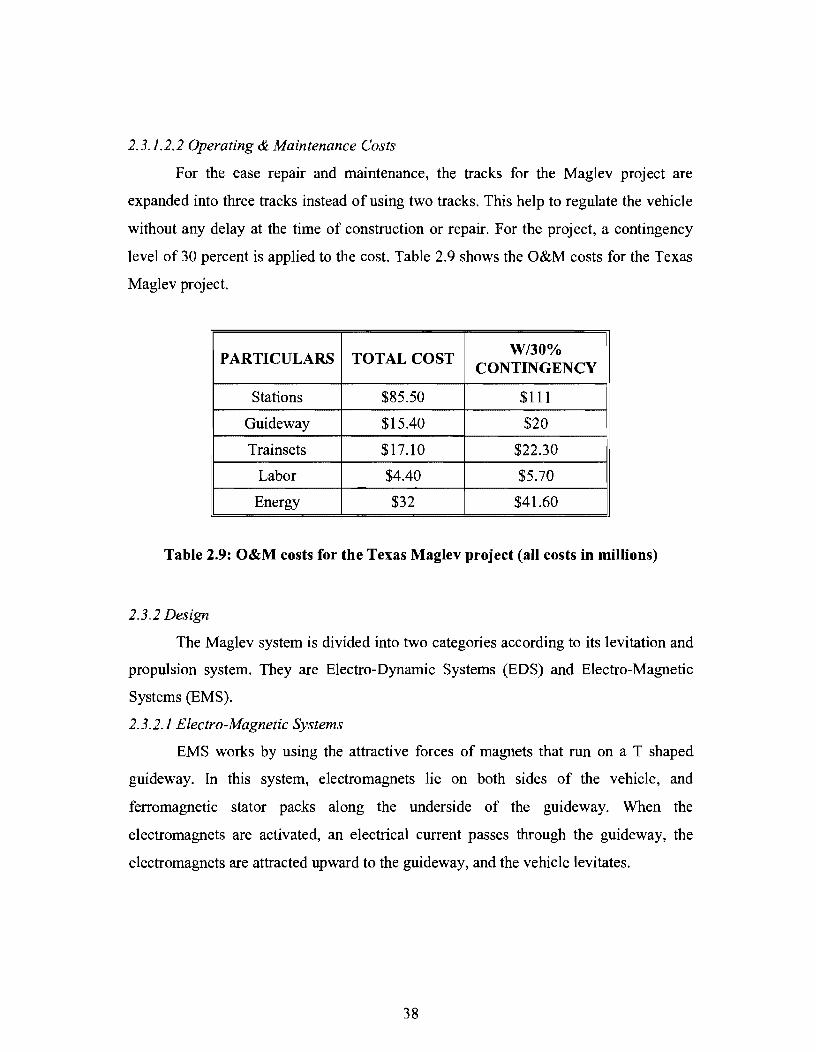
2.3.1.2.2 Operating & Maintenance Costs
For the ease repair and maintenance, the tracks for the Maglev project are
expanded into three tracks instead of using two tracks. This help to regulate the vehicle
without any delay at the time of construction or repair. For the project, a contingency
level of 30 percent is applied to the cost. Table 2.9 shows the O&M costs for the Texas
Maglev project.
PARTICULARS TOTAL COST W/30% CONTINGENCY
Stations $85.50 $111
Guideway $15.40 $20
Trainsets $17.10 $22.30
Labor $4.40 $5.70
Energy $32 $41.60
Table 2.9: O&M costs for the Texas Maglev project (all costs in millions)
2.3.2 Design
The Maglev system is divided into two categories according to its levitation and
propulsion system. They are Electro-Dynamic Systems (EDS) and Electro-Magnetic
Systems (EMS).
2.3.2.1 Electro-Magnetic Systems
EMS works by using the attractive forces of magnets that run on a T shaped
guideway. In this system, electromagnets lie on both sides of the vehicle, and
ferromagnetic stator packs along the underside of the guideway. When the
electromagnets are activated, an electrical current passes through the guideway, the
electromagnets are attracted upward to the guideway, and the vehicle levitates.
38

2.3.2.2 Electro-Dynamic Systems
EDS works by using the repulsive forces experienced by two magnets in close
proximity to each other. The trainset is then propelled forward via a charge run along
the track. One particular advantage of EDS is that the system inherently requires many
components to be integrated into the guideway. It is also an ideal time to integrate linear
synchronous motors into the guideway. LSM motors are the preferred motors for high
speed Maglev systems. The EDS system runs on a V-shaped guideway.
2.3.2.3 Trainset
The vehicle has two end sections and usually four to eight middle sections.
Although the body design varies according to the end use (passenger, cargo), the
undercarriage and all remaining components are identical. Each end section is fitted
with a driver's compartment, vehicle on-board operation control system and the payload
area for passengers, cargo, or freight. Middle sections are similar in overall composition
to end sections but do not have the driver's compartment and on-board Operation
Control Systems (OCS). Dimensions of typical Maglev trainsets are shown in
Table 2.10.
PARAMETERS I END SECTION MIDDLE SECTION
Length 26.99m 24.77m
Width 3.7Om 3.70,
Height 4.16m 4.16m
Empty Weight 48.0t 47.0t
Payload capacity 14.0t 17.5t
Total weight 92 + 2 wheelchairs 126
No. of seats 62.0t 64.5t
Table 2.10: Transrapid trainset dimensions [Transrapid]
39

The dimensions of the sections of the Transrapid maglev train are shown in Table 2.11
as follows:
PARAMETERS 2 SECTIONS 6 SECTIONS 10 SECTIONS
Length 53.98 m 153.06 m 252.l4m
Empty weight 96t 284t 472t
Payload capacity 28t 98t 168t
Total weight 124t 382t 640t
No. of seats* 128-184 up to 688 1192
Table 2.11: Dimensions for different sizes ofthe Transrapid trainset
2.3.4 Guideway
The guideway is manufactured from welded steel or reinforced concrete beams
and reinforced concrete supports and foundations. The guideway track gauge is 9.2 feet
with a double track center-to-center distance of 16.7 feet when speeds are up to 310
mph. The minimum radius of curvature is 1148 feet. At 186 mph, the radius increases to
1.0 miles. When the trains are a maximum speed of 310 mph the radius of curvature
will increase to 2.75 miles. Guideways can be elevated or at-grade. There are two
designs for elevated guideways and one design for the at-grade guideway, standardized
by Transrapid. The cross section of these different types of guideways is shown in
Figure 2.4.
40

Type III
Type II
Type I
Figure 2.4: Elevated and at-grade guideway design [Transrapidl
2.3.4.1 Elevated Guideway
The standard elevated guideway beam is from 25 m to 62 m long. The height of
the guideway ranges from 2.2 m to 20 m without special civil structures. An additional
civil structure such as a bridge is needed for the height to reach 20 m or span 31 m or
above. The guideway track is typically constructed on the foundation with individual
substructures of one column per track. A minimum guideway height of 6.7 m is
required for an overpass so that truck traffic can pass underneath. The substructure of
guideway is designed to meet the local traffic, environmental, and earthquake standards.
41

Transrapid has 2 designs for elevated guideways, namely Type I elevated and Type 2
elevated.
2.3.4.2 At-Grade Guideway
The at-grade guideway beam is 6.2 m long and has continuous foundations. The
height for at-grade guideway is from 1.35 m to 2.20 m high. The at-grade guideway has
fixed foundations as bridges, tunnels, stations. The total weight for a 6.2 m long steel
guideway beam is 9 ton. Table 2.8 contains the three different types of guideway
structures and their specific dimensions.
2.3.4.3 Switches
Bendable switches are used to allow low and high speed transfer of trains from
one track to another without stopping or waiting. The Transrapid switches consist of
special steel guideway beams that are elastically bent using electromechanical setting
drives to effect the turnout position. Transfer tables move parallel to their original
position using electromechanical drives to allow revenue trains or maintenance vehicles
to access to multiple tracks. Figure 2.5 is a picture of the Transrapid switch.
I * tt· if if 1t ft it 1t ,.. 14S.8m
Hgh-speed Bending Switch
Fig 2-5: Guideway bending switches
42

2.3.5 Levitation
The propulsion uses electro magnetic forces to levitate the trains to a 3/8 inch
gap. Levitation is maintained by long stator packs embedded in the guideway and
magnets on the train. The vehicle guideway is aT-guideway where the vehicles wrap
completely around the track. The trains are automatic and computer controlled using
control systems that are transmitted to the trains using digital radio transmission (38
GHz). Figure 2.6 shows the vehicle undercarriage components for a Transrapid system
and the framework for levitating the trainset.
Figure 2.6: Vehicle undercarriage components
2.3.6 Propulsion System
Based on German Transrapid system, the propulsion and braking use
synchronous longstator linear motor. The motor produces an electromagnetic traveling
field that propels the vehicle along the guideway. Ferromagnetic stator packs and three
phase stator windings are mounted on both sides along the underside of the guideway.
With the help of converters in substations along the route, the amplitude and frequency
of the alternating current could be changed allowing the vehicle to accelerate smoothly
from standstill to full speed. By slowing down the traveling field, the motor becomes a
43

generator and the vehicle is smoothly stopped without contact. If the public power or
propulsion system failed, independent backup brakes in each vehicle section stop the
train in the next available stopping area.
The propulsion components were fitted along the route according to the local
topography and performance requirements. The substations are installed at intervals of
6-31 mile along the route based on the train interval, speed profile, and load factors. In
addition, the substations contain energy supply components, maintenance personnel,
and spare parts. The substations receive 23 kV power from the energy supply system
and convert it into the proper format to propel the train. The propulsion control system
both controls and monitors the position of the train at all times.
The route is divided into propulsion segments through the spacing of the
substations. Each propUlsion segment is divided into smaller motor section, usually
between 0.31 mile and 1.24 mile in length. The longstator windings on the right and left
sides of the guideway are fed independently from the substation and physically offset
with respect to each other. This helps to smooth the transition between motor sections
and even if one side fails, the other has sufficient reserve to propel the train through the
segment. Wayside switch stations switch propulsion power from one section to the next
as the Transrapid train proceeds. The propulsion power is independently supplied by the
substation converters to the longstators on the right and left sides of guideway. If an
individual converter fails, or even the entire substation fails, the next substation can
provide power in its place, thereby allowing the vehicle to reach its destination.
2.3. 7 Substations
A substation could have up to 4 propulsion blocks, one per track per direction,
depending on the track layout. For the project, there will be 2 high powers, 1 medium
power, and 1 low power propulsion blocks installed.
The wayside equipment provides the feedback from the substations to the
individual propulsion segments. It includes switchgear, cables, two longstators motor
winding (right and left) with stator packs underneath the guideway, and the switch
stations. The feeder line switchgear connects or disconnects the propulsion block from
44
the route components and ensures the safe interruption of the braking energy flow
during a safe shutdown of the propulsion system.
The cables connect the converters in the propulsion blocks to the stators and
supply energy to the various wayside components. The cables are normally laid in one
cable trench for single-track guideway and one or two cable trenches for double track
guideway.
The stators consist of the laminated steel stator packs bolted to the underside of
the guideway, the three phase longstator windings mounted to the stator packs, and the
connection cabling to the switch stations. Since the stator packs are physically bolted to
the guideway beam, they are included in the guideway system. The three phase stator
windings are prefabricated aluminum cabling formed together and mounted in a
grounded harness to the stator packs.
2.3.8 Speed
The design speed of the Maglev is 340 mph with an operating speed of 31 0 mph.
The operational train headway is 5 minutes and is dependent on the number of stations
and track alignment. Because the technology is not the limiting factor, the train's
acceleration and braking can be set by the comfort conditions placed on the system by
the operators. During normal operation the trains accelerate and brake with similar
values. However during emergency braking the trains can increase the braking values
and still maintain a comfortable deceleration. Ride comfort parameters include a typical
acceleration less than 3 ftls2 and a typical braking less than 2.5 ftls2. Vertical
acceleration is limited to 2ft/s2 in a crest and 4 ftls2 in a sag curve.
2.3.9 Power
Power requirements are dependent on the number of sections, and the speed that
the train is traveling. For a ten section train power requirements are 16.1 MW at a
constant speed of 250 mph. The power is brought to guideway via substations located
along side the track. The propulsion force is powered by the substations while the train
car's onboard batteries power the levitation and guidance magnets. The batteries also
power the environmental controls, lights, and controls. However, when the trains travel
45

at a speed less than 50 mph, or are stopped at a station, the power is supplied from a
power rail that is located along side the guideway. At speeds above 50 mph, the
batteries are charged by a magnetic field that causes power to be induced into the car
batteries.
The 23 kV of electricity required for the internal energy supply and propulsion
system is drawn from the public power grid. The energy power system contains high
voltage switching equipment to connect to public grid. It also contains input
transformers, medium voltage switch gear, compensation and filtering equipment, route
power supply for wayside equipment, and control system for the energy supply
equipment. The energy supply system is installed in the substation.
2.3.10 Operation Control
The fully automated Operation Control System (OCS) controls all aspects of the
Transrapid operation. The OCS utilizes a radio based signal which is safer than a human
based operating system. The OCS maintains the train's speed within the operating
specifications and provides a safe and unobstructed travel path.
2.3.11 Communication Control Technology
The radio data transmission systems operate at 38 GHz. It also transmits the
communication signal from the vehicle to the central operation facility and vice-versa.
There are two vehicle control systems on board that are connected to separate antennas
on either end of the vehicle. These antennas connect with radio transmission masts set
at 1.25 mile intervals along the guideway. The OCS also collects maintenance and
failure information. This information is then sent to a maintenance archive and
scheduling system at the Central Maintenance Facility. The control of the Transrapid
system is divided into safety-relevant and non safety-relevant functions.
46

CHAPTER 3
ANAL YSIS OF ALTERNATIVES
3-1 Highway
Texas is considered to be the crossroads of North America because it
accommodates 79% of all US-Mexico trade traffic. As international traffic increases as
a result of the North American Free Trade Agreement, and population increases at
30,000 residents per month, the existing road and bridge system will not be sufficient to
serve the projected traffic volumes on IH-35. These high truck traffic volumes also
deteriorate the conditions of the existing roadways much faster than passenger vehicles,
according to TxDOT.
The TTC will provide a route for cross-state travel without passing through
metropolitan areas. There are several advantages to removing through traffic from the
city. It will relieve congestion on existing roadways, improving conditions for intercity
commuters and highway maintenance. It will also remove hazardous materials from
densely populated areas and improve air quality by reducing emissions in the city.
[TxDOT]
The fundamental design of the corridor is the separation of passenger vehicles
and trucks by divided lanes. Each section will have sufficient structural capacity such
that only overlays and surface texture maintenance will be required throughout the
design life of the corridor. [TxDOT]
Trucks that are transporting goods and commodities through Texas will have
two exclusive 13 foot lanes on a 42 foot wide roadway section that is designed to handle
severe loads. This will relieve congestion, allowing for faster and safer travel, as per
TxDOT. Passenger vehicles will have three 12 foot lanes on a 56 foot wide roadway
section, and will also benefit by faster and safer travel.
The IH-35 corridor is restricted in many locations by urban growth and cannot
be widened. If the required capacity cannot be met it does not make much sense to
spend state highway funds to replace a highway that will not improve congestion. The
47

TTC can provide an alternate route for through traffic and relieve the load on the
existing system. Also, monetary incentives from the federal government are promoting
research for alternatives to existing highway systems and TxDOT should not miss this
opportunity to receive federal funds.
Americans have seen tremendous changes since the authorization of the
Interstate Highway System in 1956. They have come to rely on the highway system to
accommodate their traveling needs. The highway section of the corridor will operate the
same as the existing Interstate Highway system, only much safer, faster, and more
efficient due to the separation of trucks and autos. This alternative will work in the
future because it is an improved highway.
Environmental and permitting issues for the TTC will be addressed in an
extensive environmental review so that adverse environmental impacts can be
minimized or avoided. Acquiring ROW cannot significantly affect planned growth or
land use, natural, cultural, recreational, historic or other resources. Nor can it relocate
significant numbers of people, involve air, noise or water quality impacts, or have any
significant environmental bearing. The impacts of the highway can most likely be
considered a categorical exclusion based on past experience of highway construction.
The costs for operating and maintaining highways consist of roadwork
operations and highway reconstruction. Roadwork cost will include all materials and
equipment required for maintaining the highway, the salaries and benefits for the
employees who perform the work, roadway striping, signing, and traffic signals, and
preservation expenditures such as crack sealing and resurfacing. Signing of the TTC
will incorporate ITS to provide drivers with current roadway, traffic, and weather
information. Examples of ITS include dynamic message signs, electronic toll collection,
traffic management centers, incident detection algorithms, and other smart systems. The
number of smart systems required for the corridor is dependent upon highway design.
Highway reconstruction costs will include the demolition and rebuilding of failed
structures. Rehabilitation and preventive maintenance on highways are covered under
Category-1 funding by TxDOT, which states that rehabilitation funds can be used for
48

highway main lanes, frontage roads, structures, signs, pavement markings, and striping.
Figure 3.1 is a graphical representation of maintenance cost for TxDOT districts for IH-
35.
-(I) c .2 .-:i c ---(I) 0 0 -; ::s c c «
$70.00
$60.00
$50.00
$40.00
$30.00
$20.00
$10.00
$-
Estimated Maintenance Costs
-Austin
1--------:::;=:;;;;;;;;;::-----------Dallas -Fort Worth
Laredo - San Antonio
+-__ ~------__ ----~~---Waro -Total
2002 2003 2004 2005
Year
Figure 3.1: Maintenance cost for IH-35 [TxDOT]
3-2 High Speed Rail
HSR has advantages in that it is faster than a car for longer distances and faster
than an airplane for short distances but with longer access time in the airports. HSR can
carry more people while using less space than an interstate highway. HSR consumes
less energy and produces less pollution compared to autos and airplanes.
HSR will only work efficiently on high speed tracks and is limited when placed
on regular rail. HSR has not been proven extensively in the US, which makes planning,
designing, and financing very difficult. HSR in Europe and Japan has been successful
connecting densely populated areas.
49

Other than the north-eastern coast, only the Los Angles-San Diego corridor has
the required population density to make HSR successful in the USA. HSR will only
move traffic from the airlines but not significantly from the highways which will not
improve the congestion on Texas' highways.'
If HSR is not installed in the TTC, then some of the potential riders will
continue to use the airline industry and IH-35 to get to the other Texas cities in the
corridor. Congestion and air pollution along IH-35 will continue to get worse. HSR
offers an option for the auto passenger to get off the highway. Doing nothing will not
improve the present situation; it will only make it worse.
HSR may not work in the future. American cities were organized around the
capabilities and the design of the car, unlike Europe and Japan which are organized
around rapid transit. The USA will have to spend enormous amounts of capital to
restructure the cities for a transit system to work. In the USA it is cheaper to travel by
car than it is in Europe or Japan. The average cost for gasoline in the USA is $1.40 per
gallon, however in Europe one can expect to pay $1 per liter or $4.80 per gallon.
In the USA we even enjoy relatively cheap air fares. This can be attributed to the
highly competitive airline industry. Air fares in the USA are approximately 20% to 50%
cheaper than Europe and Japan for the same distance traveled, with the exception of
NYC to Washington, D.C.
The recent history of passenger rail in this country has not been favorable for
HSR. Amtrak's ridership in this country has been low throughout its 31 years. Most
people that travel routes served by Amtrak would rather drive or fly. This is due to the
longer time that it takes to travel by rail thus affecting people's perception of rapid rail.
Amtrak has failed to operate without receiving huge sums of government subsidies.
With the economy in the state that it is in, it will be harder for HSR to find the funding
that it needs in Washington, D.C.
HSR train sets were designed to carry passengers and not freight. HSR trains
were designed to be light so that high speeds could be attained. This study found no
1 High-Speed Rail, Forth Worth
50

sources that have looked at and/or published any information regarding moving freight
on HSR. HSR will have to comply with all aspects of the National Environmental
Policy Act (NEP A). This alternative will have to address: air quality impacts, water
quality impacts, protected species, soils and unique geological features, hazardous
waste, noise, vibration, impacts on wildlife habitat and vegetation, archeological and
historic sites, land use, governmental plans and polices, utilities, public services and
facilities.
The life cycle for the system is 30 years. With routine maintenance the structure
will be repaired as needed. The cost of the repairs to equipment and infiltrator are based
on their usage, estimated by per train mile projections. Table 3.1 shows estimates per
year in 2020 given occupancy at different capacities. The design uses 50% capacity
because it was found to best represent the usage over the entire day taking into account
peak periods.
The maintenance costs are the largest portion of life cycle costs at about 60% of
total operational cost. Fuel and energy consumption is roughly 15% of the operating
budget. All costs are a factor of how many trains will make the trip during the year.
This factor is very difficult to estimate with accuracy. The estimated ridership is 1.75
million people in the year 2020. This number was found by looking at the projected
market share that HSR would have multiplied by the current travel volumes of car and
air. The totals were then projected to the year 2020 using a 3.13% growth factor. The
break down of operating cost multipliers is found in the cost section of HSR.
The costs of on-board services are to be covered by the sale of food and drinks
on the train, as well as the contractor's profit. Parcel services will also supplement the
operating cost. After the initial investment in the projects capital is repaid, HSR will
provide a profitable stock to its investors. Ticket sales along with parcel service will
contribute to $90 million in annual income.
51

3-3 Maglev
Maglev is a high speed option that could connect the major cities across the
state. It would allow travel between all the stations along the corridor. With a traveling
speed of up to 300 mph, this alternative is also the fastest. Maglev trains would be able
to quickly run cargo along the corridor. The only difficulty with moving cargo would be
breaking up the weight to allowable loads per car.
The Maglev system would greatly reduce travel time between the densely
populated areas in Texas. Ifwe were to do nothing, the heavy trucking would still occur
on IH-35 and the highway would continue to require regular maintenance. If the current
trucking loads on IH-35 continue, it will wear out its useful life, and a new stretch of
highway will have to be built much sooner than it should. This new highway will likely
continue the pattern of high maintenance and also drastically undershoot its design life.
For such a heavy shipping route, the Maglev system will likely have to have extra
strong foundations and a very tough guideway, but it will not have to undergo the
constant repairs and resurfacing the current highway does. The Maglev guideway could
more easily meet an adequate design life and, although expensive, would be easier to
replace after the design life is exceeded. There is not really a do nothing alternative
because the current traffic on IH35, which this design corridor would relieve, will
require replacement.
There is no doubt that Maglev is far superior to any other currently existing
ground surface transportation technology. They require less maintenance and are much
more energy efficient. In the future, the Maglev systems will likely operate much better
than now. Even a few systems in operation will also start a rapid decline in price and an
increase in the quality of the system. Maglev is a new idea not yet in service, and holds
great potential for the future.
Maglev offers a dramatic savings in time. It is common for traffic engineers to
view inaccessibility in units of travel time as opposed to distance. A shop that is 15
minutes and 10 miles away via mainly highway high speeds is just as likely to be visited
as a shop 2 miles away via a heavily congested collector road.
52

Due to the length of the proposed corridor, the differences in characteristics of
land environmental and permitting complications cannot be easily defined. The most
noticeable complications, nonspecific to land, are noise and visual pollution that an
elevated Maglev train will produce. However, the visual pollution that the elevated
track will produce will be minimal because the route alignment will be outside of the
major urban areas, and will only become a problem when the track enters an urban area
to pick up passengers at stations. As with visual pollution, the noise pollution will only
become a problem when the alignment reaches an urban area.
Permitting complications arise due to the development stages of Maglev;
however, it can be assumed that the guideway is comparable to a bridge with respect to
permitting.
3.3.1 Capital cost estimate
The capital cost is estimated by referring to the cost of the Baltimore
Washington Project reported in June 2000. The capital cost is expressed in year 2000
dollars that includes engineering, design and construction management, spare parts, and
training cost. For the project, the ROW, and land acquisition cost are not included in the
estimation. All the costs are escalated at 2.81 % per year to 20 I O.
All costs required to construct and operate the system are included in the
estimate. The costs include vehicles, propulsion system, energy supply, operation
control system, communication technology, guideway infrastructure, civil site work,
stations, operation and maintenance facilities, documentation, training, and initial spare
parts. The technology and systems costs are derived from the testing of Transrapid
based design over the last 25 years. The Maglev technology for this project uses the
TR08 Maglev Vehicle, and all of the associated propulsion, energy supply,
communication, and control systems for operation of the vehicle. The local pricing for
labor for the project is estimated for the civil structure and site work. The quantities of
the materials required for the project is based on the structural and foundation design
requirements. The guideway includes all substructures and superstructures. However,
the guideway excludes any required river crossing, embankment, earth excavation, and
53

tunnels that are roughly estimated as miscellaneous cost under the guideway
infrastructure.
For repair purposes, the tracks for the Maglev project are expanded into three
tracks instead of using two tracks. This helps to regulate the system so that no delay
during repair of the guideway will be experienced.
There are 318 seats per Maglev train, and estimated cost of $23.1 million. Thus,
the estimated cost per seat is $72,000. The guideway infrastructure for 400 miles comes
to 78.7% of total capital cost. The guideway infrastructure per mile per lane is
calculated to be $12 million. The total guideway cost amounts to $6.2 billion for the
entire corridor.
For the project, contingency level of 30 percent is applied to the cost. The total
cost for the Maglev Project from Dallas Forth Worth to Laredo, Texas came out to be
$18.5 billion for 3 tracks. The contingencies approximately added $5.4 billion to the
neat construction cost. Table 3.1 gives a brief summary of the costs of building the
guideway, keeping in mind the contingencies.
DESCRIPTION COST(BILLIONS)
Capital cost subtotal $16.0
Design & Construction Fees $2.4
Neat Construction total $13.1
30% contingency $5.3
Total with 30% contingency $18.4
Total with 2.81 % escalation to year 2010 $24.1
Table 3.1: Capital costs escalated to year 2010
Maglev systems have an estimated project life of 50 years. This number is taken
from the typical project life of bridges. Maglev systems inflict little damage to the rail
and surface as it is a contactless technology. The structure does still suffer from taking
54

the cyclic loadings as trains run across it. Because Maglev structures are typically
elevated, sometimes only 5 feet, and the lifetime damage to the elevating substructure is
very similar to that on a bridge. Over this project life, there will be some extra costs for
maintenance and repair, operation, and labor. The estimated values for 2020 in these
areas are discussed below. All of these numbers are derived from calculations made on
the California inter airport system. Using that projects estimated costs for the year 2020
and estimated ridership, a cost for each seat mile traveled on a Maglev system was
approximated. The calculations assumed that the yearly travel for the other system
averaged out at 85% occupation for the year. These cost per seatmile values were then
used to estimate this projects operation and maintenance costs for the year 2020.
Repair and maintenance are the big selling point for Maglev systems. Because
the trainset do not touch the guideway surface, except for small distances in EDS, there
is negligible damage to the guideway. The same is true for the trainset in that the
friction and scraping of contact does not take place. A majority of the repair on Maglev
will be on the components that do take forces. These are primarily the magnets, both on
the train and in the track, which do take the loading weight and then distribute it via the
substructure to the foundation. The loading and unloading on the track magnets can
wear on the concrete and casing that holds it in place in the structure. The trains' on
board magnet supports have to be designed to take prolonged heavy prolonged forces,
as if there was a wheel that made surface contact there. A portion of the repairs will also
take place on the train car's surface. The cars are taking heavy loads form the air drag
due to traveling at 300 mph. Both the train car surface and all the system's magnets
have to be checked regularly to make sure that they are operationaL A lot of the costs
come from these routine check-ups. As Maglev systems develop around the world, the
repair costs for materials and likely labor will begin to drop. The estimated maintenance
cost for the year 2020 is displayed in Table 3.2.
The operation costs shown in Tables 3.2 and 3.3 are broken down into energy,
labor, and total operational costs. The labor cost does look relatively low, but
considering the trains operation is primarily automated, the only real labor costs are
55

from monitoring the train's progress both on-board and off-board and the servicing
staff. In addition to the fact that the train travels at 300 mph not giving a lot of time per
trip for staff to accumulate hours. The energy costs were also surprising in that they
were quite high. It is likely that on this project, the costs may go down as the average
distance between stops is greater allowing for an overall higher average speed and
lower energy use per mile.
DESCRIPTION COST PER COST PER SEAT-MILE YEAR(MILLIONS)
Guideway $0.0110 $15.4 Maintenance
Equipment $0.0122 $17.1
Total $0.0261 $36.6 System
Labor $0.0031 $4.4 Operations
Energy $0.0028 $32.0
Grand Total $69.1
Table 3.2: Estimated O&M costs for the year 2020
O&MCOSTS UNIT COST PER
QUANTITY COST PER
UNIT(MILLIONS) YEAR(MILLIONS)
$9.8 5 $49.2 $6.1 5 $30.5 $0.3 5 $1.5
$14.3 N/A $14.3
$2.7 $2.7
Table 3.3: Overall maintenance costs for the year 2020
56

3.4 Intangible Benefits
3.4.1 Noise Reduction
Like many other environmental impacts, Maglev systems would reduce and
centralize the noise pollution. The noise from Maglev is generally based upon the
aerodynamics of the train, because the noise from the propulsion and levitation
components is virtually non-existent. An object traveling at 300 mph does make a
significant amount of noise. Anyone who has ridden in an airplane has heard the sound
of air resistance at 500 mph or above. While Maglev will not be quite as loud, it will be
barely elevated off the ground, and thus make noise pollution significant around the
guideway. The major advantage though is away from the track. The noise will be
centralized around the individual train sets, the advantage is that the noise is condensed
into spaced out sets that come and go very quickly. Also most Maglev designs don't
operate at full speed in densely populated areas. If the Maglev train is centered in the
ROW, the remaining distance will act as a buffer to the surrounding areas.
3.4.2 Hazardous Cargo
The routes will be located away from densely populated areas. Elaborate
monitoring systems intrinsic in Maglev will also assure that it is much safer than
through the local highways or traditional HSR. Compared to cars, trains in general have
fewer accidents. The monitoring systems and the wrap around guideway make Maglev
significantly safer than other modes. The primary drawback of using Maglev for
hazardous cargo is that at speeds up to 300 mph an accident would drastically increase
the possible area requiring containment.
3.4.3 Travel Time
In the modern world one of the most prized commodities is time, which is why
Maglev systems are expected to succeed. Maglev services could be charged at the cost
of transport plus the time savings. Transportation engineers commonly use travel time
as a description of distance. Compared to automobiles on the highway, Maglev would
operate at least 4 times as fast. That is a 75% reduction in travel time. While that would
not matter much for short trip, but it means that a person could travel from Dallas to San
57

Antonio in an hour as opposed to 5 hours. It is common for businessmen to travel
between Dallas and Fort Worth for business meetings; Maglev would also make it
feasible to travel to Austin or San Antonio for a meeting as well. The cost to ride a
Maglev system and ingress-egress time would be key factors in such usage.
3.4.4 Creates Jobs
The creation of a larger arterial through Texas will require workers to operate,
manage, and repair the stations and train sets. The jobs that would be adversely affected
would be other transport systems. Air travel would still dominate the long distance
travel; trucking companies would still have to transport the cargo to and from the
stations. The drivers would have a less congested route to carry their goods across the
states, even during peak traffic hours.
The biggest impact would likely be smaller air carriers that cover the planned
corridor routes, where cost and freedom of travel would likely affect the impact on the
system. Busing companies may also feel a smaller impact, in part because they would
also be able to use the system to move people. They may also restructure their operation
by configuring smaller routes to bring people to transit stations.
3.4.5 Increased Trade
The TTC has the potential to make transport cheaper. This would allow
companies to ship farther for the same price, or save money on the current shipping
price. It would also effectively reduce the distances between suppliers and consumers.
Not only is the transportation cheaper and faster, but the ability to meet face to face
would also increase. By making trade easier and cheaper in the state, the overall trade in
the state will increase.
3.4.6 Increased Safety
Maglev has two major concerns: it can move at 300 mph and it is not in direct
surface contact. For these reasons, the trains are highly monitored. Maglev guideways
are operated only one way at any given time, as it would catastrophic if two trains
collided head-on at 300 mph.
58

Maglev systems are also operated by a central control station as monitored by an
onboard conductor. This means that trains on the same track would be operated by one
system, and would continuously communicate between all trains on the same stretch of
rail. Although Maglev could be operated without an onboard staff, the trains are
typically manned to monitor the train's conditions and the track conditions.
While Maglev typically operates at comfortable decelerations, it is possible for a
train to stop extremely fast. A Maglev train traveling full speed could come to a
complete stop so quickly that it would likely be fatal to some passengers. Although if a
guideway has been discovered to be damaged such that the train may derail, it could
make that stop to prevent derailing risking only a few passengers. The fatality rate
would be much less, and repairs would be cheaper than a 300 mph derailment.
Maglev guideways are generally designed to prevent derailment or tipping. For
instance, EMS systems operate on a T-shaped guideway. The trains actually are
wrapped around the guideway. The train can glide and bump along the sliders on it, but
cannot leave the guideway without substantial damage to either the train or the
guideway or the train itself.
3.4.7 Centralize the Major Maintenance Needs
The biggest damage to our highways is the heavy cyclic loadings the road
experiences as large trucks pass over it. These loadings weaken the roadway all the way
to the foundation over time. On a highway with a large amount of trucks, like 1-35, the
surface often takes a beating and requires regular maintenance and resurfacing.
The typical damage starts as the sub-surface portions of the road settle creating a
dip in the road surface. From there it is just a matter of time before the surface begins to
break apart. Without repairs, the damage will develop into potholes, which are
devastating to vehicles at highway speeds.
With Maglev, the train does not contact the guideway surface, and therefore
reduces the damage to the guideway. The structure does undergo a heavy cyclic loading
fatigue that reacts similarly to a bridge, but does not require as much structural
59

maintenance due to the more uniform distribution of the load. These structures will
eventually need to be completely replaced.
Most of the required maintenance is generally in the elevation and propulsion
systems. Guideways require repair when damaged by an outside force, an example
would be if a train contacted the guideway with its skids. There is not much that can be
done about repairing or maintaining the damage form the heavy cyclic loads.
Carrying cargo on Maglev is effective at accumulating weight and redistributing
it since the weight from multiple trucks can be loaded onto one train creating one
effective loading cycle. Magnets allow for a more uniform distribution of weight versus
using wheels. The current weight requirements for cargo on Maglev would also mean
that the structure would undergo less stress than the typical heavy truck.
3.5 Implementation Risks
3.5.1 Trucking
The trucking industry may reject the proposal due to the toll facilities
established on the highway, even though the toll road may save the trucking companies
money in the longer run. If trucks are forced to take the new corridor instead of the
existing facility, their lobbyist may challenge the proposed relocation oftrucks.
3.5.2 Rail
The Governor's proposal of including freight lines would receive backlash from
rail industry because it competes with present rail businesses in the proposed corridor.
The rail industry would find this threatening to their current commerce in the rail
network. They would see this proposal as unfair competition from a government owned
rail line, which would receive government subsidies, and would lobby heavily against
the plan. HSR is unable of running freight at this time. The infrastructure needed to
accommodate such weight at high speeds is not possible without a more stable train to
track connection, like that of the Maglev.
60

3.5.3 Airlines
The Texas High-Speed Rail Authority is representative of what this project can
expect from its opponents. The Texas TOV faced scrutiny from the courts, where
Texas-based Southwest Airlines launched three lawsuits against the Texas High-Speed
Rail Authority. These lawsuits showed the true combativeness that the new rail would
bring to the market. Southwest Airlines was attacking the proposal in a public forum, as
opposed to the behind the scenes political tactics. This aggressiveness makes it clear to
the identity of the opposition... Southwest Airlines, which since deregulation has
consistently performed as America's most profitable air carrier, correctly perceived
much to be at stake in another travel mode's arrival in its home state.
In the routes to be serviced by the Texas Triangle Southwest Airlines has a 44%
share of the Airline market. They would have the most to lose by the instillation of an
alternative mode of transportation. Feldman reported that at the time, 6.6 percent of
Southwest's total traffic was either originating in or destined to the cities that Texas
TOV would serve and that 26.7 percent of Southwest's passengers flew to or from
Texas, where 180 out ofthe carrier's 1,400 daily flights originated. Little wonder, then,
that Southwest viewed Texas TOV as "enemy No.1" and fought the project "down and
dirty." [Perl]
Southwest's outspoken chairman, Herb Kelleher, did not mince words, or
threats, regarding his opposition to the Texas TOV. Calling high-speed rail supporters
"economic illiterates," he went on to challenge Texas TOV's claims head on:
"They are saying that the roads and airways will so
congested that the train wi 11 the t al ternative ... So
I have no ambition, no imagination, and no ingenuity." "If
that's the case, I'll just buy some 757s and double the
number of seats between Houston and Dallas. The whole
thing is just so ludicrous!"
Southwest's current structure of using a standard airplane for all of its routes
would make it difficult for such an expansion to 757s. An additional tactic was used
61

when San Antonio mayor Nelson Wolff floated the idea of using improvement fees to
provide rail access into his city-owned airport. To this news Kelleher publicly
threatened to pull all of Southwest's flights out of San Antonio. These accounted for 30
percent of San Antonio's scheduled air service. Kelleher told a meeting of his own
employees that if the Texas TGV obtained any assistance form the municipality," San
Antonio could become a train town instead of a plane town." [Perl]
It is difficult to tell which side truly won in the litigation brought against the
Texas TGV A. Even without winning in court, Southwest's legal actions had put Texas
TGV's required fundraising behind schedule. Helen Ng reported "Congressional
pressure helped to kill a federal subsidy for Texas TGV, because it was allegedly
damaging to Boeing's friend and customer, Southwest Airlines." [Perl]
Texas TGV's "investment grade" ridership forecast by Charles River Associates
helps to explain why Southwest Airlines and its colorful chairman devoted so much
effort to battling a mode, which was publicly disparaged as an unworthy competitor.
This study predicted that Texas TGV's lines would carry 14 million people and
generate $618 million in annual revenues by 2010. Diversion of traffic from other
modes ranged from 21 percent to 31 percent, among five different scenarios, leading
Charles River Associates to note, "This is a very significant travel impact for a single
new transportation facility serving a large existing market; it will have important
impacts on the amounts of air pollution and energy consumption involved in
transporting intercity travelers in Texas, and it will have potentially significant impacts
on the congestion levels at airports and on interstate highways in future years." [Perl]
3.4.4 Public Use
Public outcry may come in many forms. Tax payers may oppose the multi
billion dollar proposal, because they may not recognize the potential financial gain for
the State of Texas. Homeowners near the corridor will lose property in order to
establish the right of way. The plan, if implemented, may approach some communities
and cause disruption with noise and construction. Business owners may challenge the
corridor if it has a negative impact on their business. Many cities will not be included in
62

the connection of the corridor and will miss out on the possible increase in commerce
opportunities.
Environmental groups may challenge the construction of the corridor in fear that
the plan will affect the ecosystem of the surrounding areas. Steps must be made in order
to minimize the negative impact on the environment. People may avoid the system if
they are accustomed to regular routes. The out of pocket cost due to toll and ticket cost
might deter commuters.
63

!!!!!!!!!!!!!!!!!!!"#$%!&'()!*)&+',)%!'-!$-.)-.$/-'++0!1+'-2!&'()!$-!.#)!/*$($-'+3!
44!5"6!7$1*'*0!8$($.$9'.$/-!")':!
CHAPTER 4
SURVEY OF FINANCING ALTERNATIVES
The TTC, being a statewide system, requires huge capital investment and
innovative forms of financing. The financing tools proposed for funding the corridor are
toll equity, regional mobility authority, and Texas Mobility Fund. Other methods of
funding suggested include concessions, federal grants, and leasing right of way. It is
beyond the scope of this study to discuss the funding alternatives for the TTC.
However, a general discussion of potential funding and financing sources for the
proposed Maglev route is presented in this chapter. The potential funding and financing
sources in sections 4.1, 4.2, and 4.3 are cited from "South East High Speed Rail
Corridor Feasibility Report" prepared by the North Carolina Department of
Transportation (26).
4.1 Potential Funding Sources for Capital Costs (26)
Funding sources are those which do not have to be repaid. They are usually used
to cover the capital costs. Such funding is obtained in the form of grants. These are
referred to as subsidies throughout this report. Sections 4.1.1 through 4.1.7 list the
various funding sources that may be available for the capital costs.
4.1.1 Federal Funds
Federal funds are the grants provided by the federal government. There are
some federal regulations that require matching grants at state and local levels for a
project to secure these grants.
65

4.1.2 State Funds
State funds are grants from the state government. The main source of revenue
for the state to fund transportation projects is through gasoline tax and other vehicle
related taxes. A part of these revenues are allocated for transportation projects. Since
many projects compete for these funds, obtaining a budgetary allocation may be
difficult.
4.1.3 Local Public Funds
Local funds are grants that do not need to be repaid, although securing local
general revenue may be difficult and depend on the project's local support.
4.1.4 State/Local Tax Revenue
A legislated tax or fee can be imposed on a dedicated revenue source. Such a tax
will provide a steady stream of revenue that can be used to pay back the capital costs.
Such a funding source is relatively stable and easy to forecast. Securing such a funding
may be difficult due to political compulsions. Any state tax used for issuing debt
requires legislation, which requires voter approval.
4.1.5 Local Value Capture Methods (Real Estate Tax, etc.)
Tax can be imposed on the revenues resulting from enhanced real estate
development due to improvements in transportation corridors. Special assessment
districts can be created for imposing real estate taxes. The funds generated would
typically cover cost for station improvements. Transportation corridors improve the
economic activity in the surrounding areas. Hence, the property tax revenue generated
66

from that area increases. Tax increment financing is the allocation of incremental tax
revenues to transportation proj ects.
4.1.6 Regional Taxation Districts
Similar to tax increment financing but on a broader scale, a regional taxation
district is established to pay for the costs of infrastructure development, often spanning
the entire region benefiting from the infrastructure. Approval of a referendum is
required only in the districts.
4.1.7 Sale or Lease of Development Rights
The property owned by the state around the new transportation corridor can be
sold or leased to a private entity for development. This would provide a steady stream
of revenues for funding the capital costs or to make payments on debts. However, the
purchase price may be lower than that could be obtained at a later stage of development.
4.2 Potential Financing Sources for Capital Costs (26)
Financing sources are those which are used to cover capital costs and have to be
paid back over a period of time. A common tool used to raise capital is the issue of
bonds. The terminology bond is used throughout this report to represent this form of
financing. Sections 4.2.1 through 4.2.9 list various financing sources for capital costs.
4.2.1 Tax Exempt Revenue Bonds
Tax exempt revenue bonds can be issued to finance the capital costs. Federal
taxes are waived on the interest income from such bonds, resulting in lower interest
rates. Tax exempt revenue bonds offer a relatively stable and guaranteed form of
financing for the capital costs. Higher total value of bonds can be issued for the same
67

revenue as the interest rates are lower than taxable bonds. Such bonds are usually
backed by dedicated tax revenue.
4.2.2 Project Finance
Revenue bonds can be issued backed solely by the revenues generated by the
transportation project. These bonds may be tax exempt or taxable depending on the
ownership of the transportation system. Since the revenues of the system may not be
stable, project financing may be considered risky by the investors. As the bonds are not
backed by dedicated tax revenues, securing such funds would have lesser political
interference.
4.2.3 General Obligation Bonds
General Obligation bonds can be issued to pay for investments in public
transportation facilities, and are backed by the full faith and credit of the state. Thus, the
risk is transferred from the project to the state. However, any excess revenue generated
would be directed back to the state. Such bonds generate relatively more interest from
the investors as they would analyze the state's credit risk before making an investment.
4.2.4 State Guarantee
Project financing can be backed by a state guarantee. The guarantee would be
effective if the revenues generated by the system are not sufficient to pay for the annual
payments for the bonds. A state guarantee lowers the risk associated with the project,
which would attract investors, and reduce the interest rates on bonds.
68

4.2.5 Export Financing
Export/Import banks offer financing for purchase of equipment, technology or
service from foreign countries. Loans are offered with favorable financial terms so that
both the vendor and the buyer may be benefited.
4.2.6 Vendor Financing
The suppliers of equipment or technology may offer financing for a project to
encourage the sales of their products. Acquiring such a form of finance often requires a
lease agreement with the supplier. Vendor financing may be used for purchase of rolling
stock, signaling systems, etc. The rate of interest for the finance may be higher than that
for tax-exempt revenue bonds.
4.2. 7 Equipment Leasing
Substantial cost savings in the financing of facilities and equipment can be
achieved in the United States through the use of a tax-oriented lease. Tax benefits can
be claimed by the lessor in the form of depreciation deductions. The lessee can get tax
benefits too, as the lease payment is deducted as an expense. Realization of tax benefits
results in lower cost of financing.
4.2.8 Private Equity
Finance for capital costs may be raised by private equity investment. This is
achieved by issuing of shares of common stock. However, the shareholders would have
some control over the project if private equity investment is used.
69

4.2.9 Loans
Loans can be obtained from commercial banks for financing of infrastructure
projects. Although these loans are typically offered for five to eight years, longer
payback periods may be secured for infrastructure projects. Commercial loans have
higher interest rates than bonds. Also, the bank would assess the risk involved before
lending for any particular project.
4.3 Potential Revenue Sources for Operating Costs (26)
Revenue sources are those funds raised as a result of the normal operation of the
Maglev service. Typical revenue sources include fare box, advertising, and on-boardlin
station concessions. Sections 4.3.1 through 4.3.5 lists the various revenue sources for
operating costs.
4.3.1 Fare Box Revenue
Fare box revenue is the main source for operating costs. The total amount of
revenue generated by the ticket price during the normal operation of a transportation
system constitutes fare box revenue. The revenue estimates depend on the accuracy of
ridership forecasts, which are often difficult to predict. The ridership depends on
various factors such as ticket price, level of service of the system, etc.
4.3.2 On-Board and In-Station Concessions, Advertising
On-board concessions would involve the sale of goods and services on the train
such as food, beverages, and telephone service. In-station concessions would involve
such sales as food, beverages, telephone service, books and magazines, parking, etc.
The space in and around the stations can be sold for advertisements. The revenue
70

generated may be used for maintenance and operation of stations. These revenues are
relatively more predictable. However, the total amount of revenue generated by
advertising may not be significant.
4.3.3 High Speed Parcel Transpart
The high speed of Maglev trains may be used for express delivery of parcels.
The revenue generated from high speed parcel transport can be used for operation and
maintenance costs. The revenue generated may not be very high as the Maglevs have to
compete with air transportation in this sector.
4.3.4 Lease afRight-al-Way
The state can lease a part of the right-of-way to railroad operators for freight rail
operations. The railroad pays the annual lease amount that would provide a steady
stream of revenue. The railroad would also take the responsibility for maintenance of
right of way for the lease period.
4.3.5 Parallel Uses afRight-al-Way
The longitudinal rights along parts of right-of-way can be leased to firms in
telecommunications, power, or gas utility industries. This would provide predictable
revenues for a long period of time.
4.4 Public-Private Partnership (Alameda Corridor) (27)
The Alameda Corridor is located in southern Los Angeles County, California,
running from the Ports of Long Beach and Los Angeles 20 miles north to downtown
Los Angeles, primarily along and adjacent to Alameda Street. The project extends
71
through or borders the Cities of Vernon, Huntington Park, South Gate, Lynwood,
Compton, Carson, and Los Angeles, and the County of Los Angeles.
The Alameda Corridor Transportation Authority (ACT A) was created in August
1989 in response to the growing concern regarding traffic congestion in the port area.
From the outset, it was designed as a freight only rail expressway to alleviate the intense
freight traffic between the Ports of Long Beach and Los Angeles. The Alameda
Corridor is operated by a partnership between the Ports of Long Beach and Los
Angeles, Burlington North and Santa Fe Railroad, and Union Pacific Railroad.
The Ports of Long Angeles and Long Beach are the two busiest seaports in the
United States. The number of cargo containers moving through the ports in 2001 was
9.6 million units. The ports project the volume of cargo containers would increase to 24
million units by 2020.
Before the completion of Alameda Corridor, there were 20 to 35 daily train trips
on the branch lines serving the ports. The Alameda Corridor is designed to
accommodate the 100 daily train trips to and from the ports projected for 2020, with
trains averaging 30 to 40 mph.
The Alameda Corridor was funded by both public and private sources including
$1.16 billion in revenue bonds sold by ACTA, a $400 million loan from the U.S.
Department of Transportation, $394 million from the ports, and $347 million in grants
administered by the Los Angeles County Metropolitan Transportation Authority. Bond
debt service will be paid through fees collected from the railroads for the transportation
of cargo containers outside of southern California (28).
72
The Alameda Corridor was the first such joint venture of its kind and
successfully demonstrated what innovative financing could do for ground surface
transportation in America. It went a long way in changing the views and inhibitions
regarding such joint ventures.
73

!!!!!!!!!!!!!!!!!!!"#$%!&'()!*)&+',)%!'-!$-.)-.$/-'++0!1+'-2!&'()!$-!.#)!/*$($-'+3!
44!5"6!7$1*'*0!8$($.$9'.$/-!")':!

CHAPTERS
FINANCIAL FEASIBILITY ANALYSIS
5.1 Selection of Route
The route considered for the study runs from Dallas-Fort Worth to Laredo and
covers a distance of 435 miles. There are three stations along the way, in Waco, Austin,
and San Antonio, and two terminals, at Dallas-Fort Worth and Laredo. Maglev trains
would be used for the project. It covers the principal cities of central Texas and runs
along the major north-south corridor through Texas, starting close to the Oklahoma
border in the north, to the border with Mexico in the south.
Certain assumptions have been made with regard to the study route. These
assumptions are as follows
• Right of way is available (cost of right of way not considered).
• Transrapid system and trains are used.
• Beginning of project - 2005.
• Beginning of operation - 2015.
• Capital investment at midpoint of construction phase (2010) has been taken
into consideration. Capital investment will be required throughout the design
and construction phase. Since a detailed time line regarding these phases is
not available, it is assumed for the calculation purposes that the entire capital
investment is made at the mid point of construction phase.
75

• The average annual inflation rate calculated for years 1991 to 2000 from the
Consumer Price Index is 2.81 %. All costs in this report are in 2000 dollars
escalated using the above value. The effect of taxes which may be applicable
is not considered. The value of 2.81 % is considered as the effective rate of
interest in all the calculations (29).
5.2 Scenarios for Financial Analysis
Costs from the BW Maglev project have been considered and used to derive the
cost for the selected route. However, the costs shown for Texas have been derived using
local guideway construction costs for concrete infrastructure. Two different scenarios
have been considered for each segment, i.e., costs derived from the BW Maglev costs
and the Texas Maglev costs. Costs have been estimated for both scenarios and presented
in the form of charts in Appendix C (30, 31). These costs were then applied to the
segment considered from Dallas-Fort Worth to Laredo.
Revenue is calculated considering current travel trends in Texas and is based on
different headway and ridership assumptions. An average ticket price has been
considered for the whole length of the route. For any project to be implemented, the
benefit to cost ratio should be greater than one. Thus, an estimation of the revenues
generated is important to derive the benefit to cost ratio.
The different scenarios considered are described below.
• The cost estimate for a Maglev system between Dallas-Fort Worth and
Laredo is derived using the BW Maglev costs in the first scenario.
76

• The cost estimate for a Maglev system between Dallas-Fort Worth and
Laredo is derived using local construction costs in Texas in the second
scenario.
The analysis is done with 30-minute headway and 20-minute headway for each
of the above scenarios.
5.3 Ridership Assumptions
Before looking into the specifics of the scenarios, it is important to state the
assumptions that have been considered for each of the scenarios.
• 16 hour daily operation has been considered.
• The relationship between ticket price and ridership is assumed to be linear.
The relationship is generally non linear and depends on several factors such
as elasticity, propensity of riders, and level of service. However, at present,
the exact relationship for this particular project is not known. Hence a linear
relationship is assumed for the sake of simplicity.
• Average ticket price for the entire route length is considered for the purpose
of analysis. The ticket price range of $50 to $100 was fixed based on the
average one-way domestic airline fares between the cities considered in the
corridor (32).
It is assumed that ridership increases if the headways are shorter, even for the
same ticket price. For the ordinary traveler, frequency of service is a very important
consideration. For example, for a ticket price of $100, the ridership is assumed to be
50% of capacity if the headway is 30 minutes and the ridership increases to 60% of
77
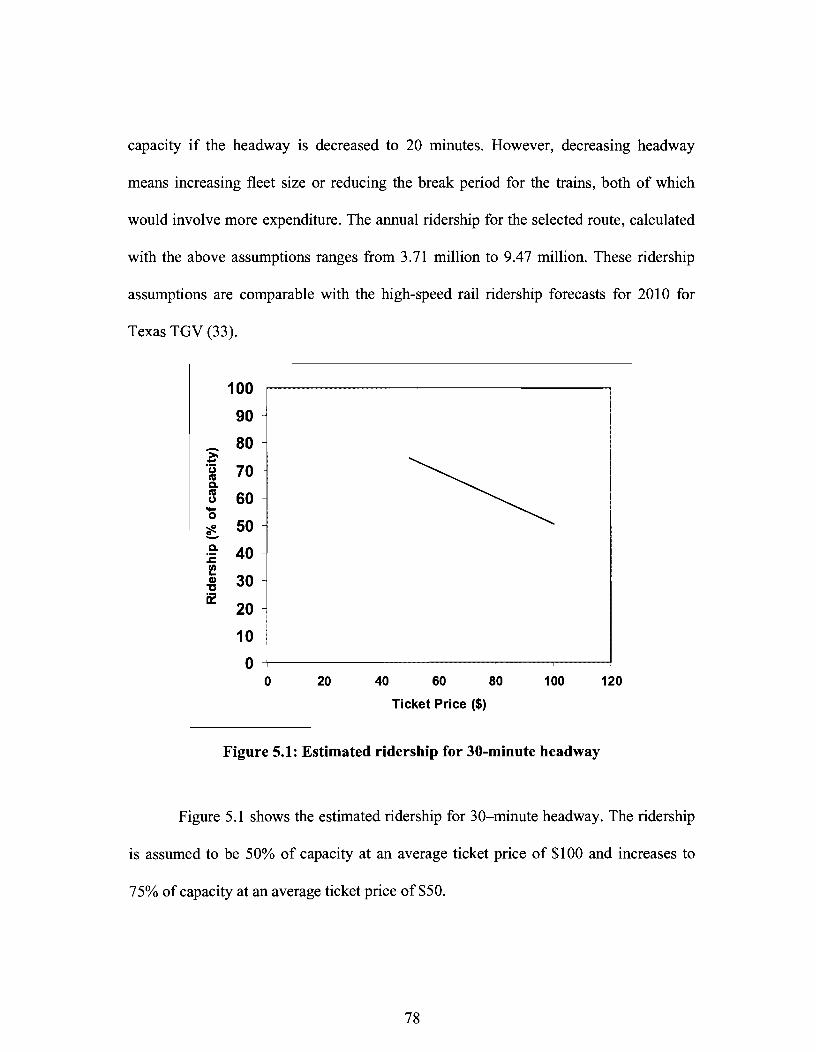
capacity if the headway is decreased to 20 minutes. However, decreasing headway
means increasing fleet size or reducing the break period for the trains, both of which
would involve more expenditure. The annual ridership for the selected route, calculated
with the above assumptions ranges from 3.71 million to 9.47 million. These ridership
assumptions are comparable with the high-speed rail ridership forecasts for 2010 for
Texas TGV (33).
100
90
- 80 ~ 'u 70 IV C. IV 60 CJ .... 0
";f!. 50 -c. 40 J:
~ 30 Q)
"C
ii 20
10
0 0 20 40 60 80 100 120
Ticket Price ($)
Figure 5.1: Estimated ridership for 30-minute headway
Figure 5.1 shows the estimated ridership for 30-minute headway. The ridership
is assumed to be 50% of capacity at an average ticket price of $100 and increases to
75% of capacity at an average ticket price of$50.
78

100
90
~ 80
'u 70 . ftI Co ftI 60 (,) .... 0
?ft. 50 -Co 40 :c f
30 &
" C2 20
10
0 0 20 40 60 80 100 120
Ticket Price ($)
Figure 5.2: Estimated ridership for 20-minute headway
Figure 5.2 shows the estimated ridership for 20-minute headway. The ridership
is assumed to be 60% of capacity at an average ticket price of $100 and increases to
85% of capacity at an average ticket price of $50.
5.4 Financial Analysis
The financial analysis is done for each of the scenarios with the assumptions
stated above. The annual payment required to repay the loan (for the capital cost) is
calculated for a 30 year and a 50 year payback period. The average annual operation
and maintenance costs are added to this payment to obtain the annual revenue required
in order to run the Maglev system and also make annual payments so that the capital
costs are recovered at the end of the payback period.
79

The revenue generated is calculated for various ridership assumptions and the
corresponding ticket price. This revenue will be used for operation and maintenance and
also to repay the capital cost which was paid for by issuing bonds or other means of
financing. Basically, the fare-box revenue is used to fund operation and maintenance
costs and to repay the bonds. The funds remaining after paying for operation and
maintenance costs can be used to repay the bonds. However, this amount is not always
sufficient to fund the entire capital costs. The remaining amount of the funds that have
to be procured is designated as the subsidies. The subsidies are funds procured through
grants that need not be returned.
The annual payment required to recover the capital cost is calculated using the
equation for uniform-series capital recovery factor given below (34).
Where
• A = End-of-period cash flows (or equivalent end of period values) in a
uniform series continuing for a specified number of periods. Here the letter
A implies annual.
• P = Present worth of money, i.e., the equivalent worth of one or more cash
flows at a relative point in time defined as present.
• i = Effective interest rate per period.
• N = Number of compounding periods.
80

For this analysis,
• i Inflation rate = 2.81 %.
• N = Payback period - 30 years or 50 years.
• P Capital cost at the middle of construction phase (2010).
• A Annual payment required to recover the capital cost.
The annual operation and maintenance cost is added to the value of A to obtain
the annual revenue requirement. The farebox revenue is calculated from the ridership
values and average ticket price. This amount is subtracted from the annual revenue
requirement to obtain the amount of subsidies required. This is explained for one
particular scenario and the sample calculations are shown below.
• Route length, L 435 miles.
• Average Speed, V 185 mph.
• Cycle time, C, is the time required for a Maglev train to complete one round
trip, C 2 * 435 /185 = 4.7 hours.
• Headway, H = 20 minutes.
• Train Capacity (Transrapid Train sets) = 318 seats.
• Hours of Operation 6 A.M. to 10 P.M. = 16 hours.
• Number of train sets required C / H = (4.7 * 60) / 20 = 14.1, i.e., 15 trains.
• Since Maglev trains have no contact with the guideway and very few
moving parts, the chances of breakdown can be expected to be low.
However, two spare trains are added to the required number of trains for
emergency.
81

• Number oftrain sets required = 17 trains.
• Capital cost derived for construction in Texas (2000 dollars), P = $18,804
million.
• Operation and maintenance cost (2000 dollar) = $175 million.
• Inflation rate, i = 0.0281.
• Payback period, N = 30 years.
Annual payment required to recover the capital cost
• A = P i(1 + i)N O+i)N -1
• A = 18804 0.02810 + 0.0281)30 0+ 0.0281)30 -1
• A = $ 936 million.
• Annual revenue requirement = 936 + 175 = $ 1,111 million.
• Ridership = 85% of capacity.
• Annual ridership = 9.47 million trips.
• Average ticket price = $50 per trip.
• Total fare-box revenue = 50 * 9.47 million = $ 474 million/year.
The fare-box revenue can be used for operation and maintenance and to repay
part of the capital cost funded by financing sources such as bonds. The remaining
amount, which cannot be repaid by the system, has to be subsidized. This amount is
designated as subsidies.
• Subsidies = 1111 - 474 = $638 million.
82

The above process is repeated by varying the capital cost, headway as follows
1. Costs from Baltimore-Washington Maglev; headway 30 minutes.
2. Costs from Baltimore-Washington Maglev; headway = 20 minutes.
3. Costs from Texas Maglev; headway 30 minutes.
4. Costs from Texas Maglev; headway = 20 minutes.
The results are tabulated in Tables 5.1 through 5.8 for different values of
ridership and average ticket price. The amount of subsidies and bonds are shown as
charts in Figures 5.3 through 5.6.
Table 5.1: Annual revenue requirements for 30-minute headway using cost estimate from the Baltimore-Washington Maglev project
Units - million $, Base Year 2000 Total Revenue Required I
O&M Annual Payment Year
Costs per 30 year 50 year 30 year 50 year Capital Cost year payback payback payback payback
35,468 155 1,765 1,329 1,920 1,484
83

Table 5.2: Different funding scenarios for varying ridership estimates for 30-minute headway using cost estimate from the Baltimore-Washington Maglev
project
Funds Ridership Annual (million $}
(%of Ridership Average Funding 30 yr 50 yr Ca,eacit.z:) ~millions2 Ticket Price Source ,ea.z:back ,ea.z:back
75 5.57 $50 Subsidies 1,641 1,205 Bonds 279 279
70 5.20 $60 Subsidies 1,608 1,172 Bonds 312 312
65 4.83 $70 Subsidies 1,582 1,146 Bonds 338 338
60 4.46 $80 Subsidies 1,563 1,127 Bonds 357
55 4.09 $90 Subsidies 1,552 1,116 Bonds 368 368
50 3.71 $100 Subsidies 1,549 1,112 Bonds 371 371
84

$1,800
$1 ,600 ~-[1!I!f-~---;;!It- -~--'--C=~~'-~-~-'-~--'---~~------~"'
$1 ,400 -H%1f----.. ~-nl___-~-IlIIi:1____~--__I!iIl___-·~___l_~-·-·fl:!I___-·-···-
~ $1,200 .2 :: $1,000 E -; $800
" c ~ $600
$400
$200
$0 , (f)
I ~ E (f)
05 i ~ 50 60
(f)
.!Q "'0
E :::I en
70 80
Ticket Price ($)
90
ID 32 (f) .0 :::I
i en 100
1.30 yr I !. 591~_
Figure 5.3: Payback scenario for headway of 30 minutes with costs derived from the Baltimore-Washington Maglev project
85

Table 5.3: Annual revenue requirements for 20-minute headway using cost estimates from the Baltimore-Washington Maglev project
Units - million $, Base Year 2000
Annual Payment Total Revenue Required / Year
0& M Costs 30 year 50 year 30 year 50 year Capital Cost per year payback payback payback payback
35,666 175 1,775 1,337 1,951 1,512
Table 5.4: Different funding scenarios for varying ridership estimates for 20-minute headway using cost estimates from the Baltimore-Washington Maglev
project
Funds Ridership Annual (million $)
(%of Ridership Average Funding 30yr 50 yr CaEaciti:) ~millions2 Ticket Price Source Eai:back Eai:back
85 9.47 $50 Subsidies 1,477 1,038 Bonds 474 474
80 8.91 $60 Subsidies 1,416 977 Bonds 535 535
75 8.36 $70 Subsidies 1,366 927 Bonds 585 585
70 7.80 $80 Subsidies 1,327 888 Bonds 624 624
65 7.24 $90 Subsidies 1,299 860 Bonds 652 652
60 6.69 $100 Subsidies 1,282 843 Bonds 669 669
86

$1,600
$1 ,400 +.i--"····~----ml-~---··-~----···--- -_ ...... _-
Iii $1,200 +mJ--~~---1_-··-___ ~-···-IIIII-------lM·~~ ___ ~-······~ c g $1,000
.§. $800
~ $600 :::I LI. $400
$200
$0
50 60 70 80 90 100
Ticket Price ($)
Figure 5.4: Payback scenario for headway of 20 minutes with costs derived from the Baltimore-Washington Maglev project
87

Table 5.5: Annual revenue requirements for 30-minute headway for the Texas Maglev project
Capital Cost
18,606
Units - million $, Base Year 2000
0& M Costs per year
155
Annual Payment 30 year 50 year payback payback
926 697
Total Revenue Required I
30 year payback
1,081
Year 50 year payback
852
Table 5.6: Different funding scenarios for varying ridership estimates for 30-minute headway for the Texas Maglev project
Funds Ridership Annual {million $2
(%of Ridership Average Funding 30yr 50yr Capacit~ ~mi11ions! Ticket Price Source pa~back pa~back
75 5.57 $50 Subsidies 802 573 Bonds 279 279
70 5.20 $60 Subsidies 769 540 Bonds 312 312
65 4.83 $70 Subsidies 743 514 Bonds 338 338
60 4.46 $80 Subsidies 724 495 Bonds 357 357
55 4.09 $90 Subsidies 713 484 Bonds 368 368
50 3.71 $100 Subsidies 709 480 Bonds 371 371
88

$900
$800
$700 -II) $600 c .2 :: $500 E - $400 II) 'tJ C :::I $300 u.
$200
$100
$0
50 60 70 80 90 100
Ticket Price ($)
Figure 5.5: Payback scenario for headway of 30 minutes for the Texas Maglev project
89
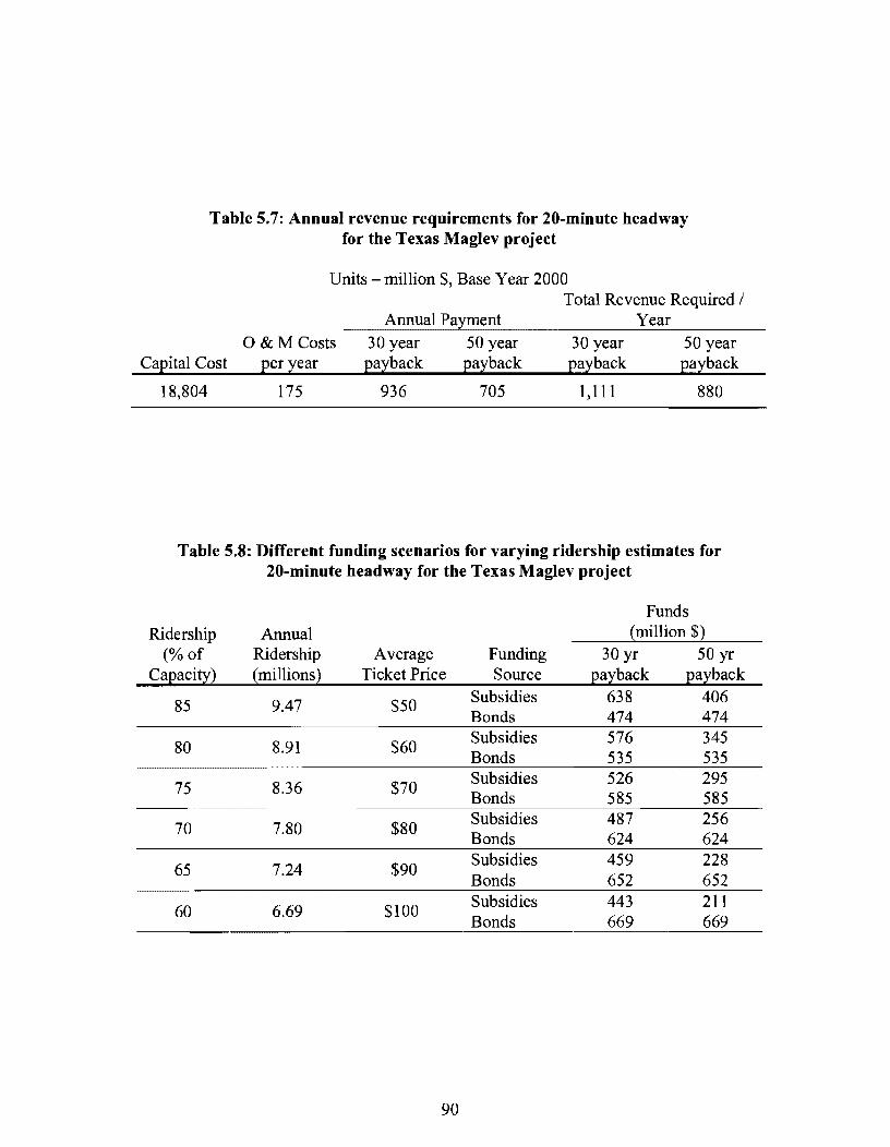
Table 5.7: Annual revenue requirements for 20-minute headway for the Texas Maglev project
Units million $, Base Year 2000 Total Revenue Required I
Annual Payment Year 0& M Costs 30 year 50 year 30 year 50 year
Capital Cost per year payback payback payback payback
18,804 175 936 705 1,111 880
Table 5.8: Different funding scenarios for varying ridership estimates for 20-minute headway for the Texas Maglev project
Funds Ridership Annual (million $}
(%of Ridership Average Funding 30yr 50 yr CaEacitx) ~mi1lionsl Ticket Price Source Eaxback Eaxback
85 9.47 $50 Subsidies 638 406 Bonds 474 474
80 8.91 $60 Subsidies 576 345 Bonds 535 535
75 8.36 $70 Subsidies 526 295 Bonds
70 7.80 $80 Subsidies 487 256 Bonds 624 624
65 7.24 $90 Subsidies 459 228 Bonds 652 652
60 6.69 $100 Subsidies 443 211 Bonds 669 669
90

$800~-------------------------------,
$700+-----------~-------------------~
u; $600 -t-I!\!!I------------'~--c o = $500 -t-I!\!!I-----~~
.§. $400
~ $300 c ~ $200
$100
$0
50
(f) Q)
:0 :2 :::l
(f)
60
(f) I (f) -0 Q) e: i :0 0 ,:2 a:l
l:::l .(f)
70 80
Ticket Price ($)
(f) (f) (f) I~ Q) -0 Q)
:0 e: :0 Ie: 'en 0
:2 :0
..c a:l .a:l
:::l :::l (f) (f)
I 90 100
.30yr
Figure 5.6: Payback scenario for headway of 20 minutes for the Texas Maglev project
5.5 Discussion of Results
The results of the analysis can be read from the charts in Figures 3.3 through
3.6. The x-axis contains the average ticket price ranging from $50 to $100 with a $10
interval. For each of these ticket prices, the amount of funds paid by subsidies and
amount of funds paid by bonds are represented in the form of bar graph, for 30-year
payback period and 50-year payback period.
Here, subsidies represent the fraction of funding that does not have to be repaid.
Bonds represent the fraction of funding that must be repaid by the revenues generated
by the normal operation of the Maglev system. The part of investment financed by
various sources such as revenue bonds has to be recovered from the system, Although
91

this is represented as bonds, there are various other financing sources as discussed
earlier which may be used to fund the capital costs.
Here is an illustrated example of reading these charts. Consider Figure 4.6
above. This represents a payback scenario for an estimated headway of 20 minutes for
the Texas Maglev project.
Suppose the ticket price is $50 and 30 year payback period is considered we can
read in Figure 4.6 that an amount of $630 million/year has to be subsidized and $470
million/year will be the revenue generated by the system which can be used to recover
the capital costs.
To find the least ticket price with a payback period of 50 years for which the
subsidies are less than 30% of total funds-
• For a 50 year payback period the total annual revenue required = $877
million
• Figure 4.6 shows that for 50 year payback period, the amount of subsidies
for a ticket price of $80 is $250 million/year which is 29% of total cost.
For this case, the ticket price has to be at least $80 for subsidies to be less than
30%. Similarly various cases can be studied by varying the attributes in the chart.
The general trends that can be seen from the Figures 4.3 through 4.6 are as
follows
• As the ticket price IS increased, the percentage of subsidies required
. decreases in spite of a decrease in ridership.
92

• The fraction of funds that have to be subsidized decreases as the total cost of
the project is decreased.
5.5.1 Sensitivity Analysisfor Effective Interest Rate
The effective interest rate used in the analysis is 2.81 %. The feasible regions
will be affected if the value of effective interest rate is varied. The feasible regions are
calculated for effective interest rates of 3%, 4%, and 5% and presented in Figures 5.7
and 5.8.
$100
$90
B 'C $80 D.. 1; ~ $70 i=
$60
I
,
i i
$50 :30 :rl-;; 1 ~o y; 1-~r 00;T 5O;13~r :5Dyr !.
• 2.81% I 3% I 4% 5% I
Effective Interest Rate
Figure 5.7: Sensitivity of effective interest rate for headway of 30 minutes for the Texas Maglev project
Figure 5.7 shows that for Texas Maglev project with 30-minute headway, there
is no feasible region for 30-year payback period. For 50-year payback period, the
feasible region decreases for 3% effective interest rate and there is no feasible region for
effective interest rates of 4% and 5%.
93

$100 ........... _--j A
$90
B $80 'i: ~ ...... ~.---
0. ... j u $70 -~-- t------t=
$60 i .............. --~
$50 ~ ~ ~,. ~,. ~
30 yr I 50yr 30 yr I 50yr 30 yr I 50yr 30 yr 50yr
2.81% 3% 4% 5%
Effedive Interest Rate
Figure 5.8: Sensitivity of effective interest rate for headway of 20 minutes for the Texas Maglev project
Figure 5.8 shows the feasible regions for Texas Maglev project with 20-minute
headway, The feasible region decreases for 4% and 5% effective interest rate for 30-
year payback period. For 50-year-payback period, there feasible region decreases only
for 5% effective interest rate.
The results are more sensitive to variation of effective interest rate with 30-
minute headway than with 20-minute headway.
5.5.2. Gas Tax Subsidies
The feasibility of the Maglev system depends on the amount of funding that can
be subsidized. In other words, the maximum percentage of subsidies that is acceptable
has to be defmed. Based on the example of Alameda Corridor, this value is assumed to
94

be 60%. A feasible solution exists only if the fraction of subsidies required for the
system to break even is less than or equal to 60%.
The subsidies are the funds that are provided in the form of grants and need not
be paid back by the system. Various funding sources are discussed earlier, one of which
is state funds. The state tax on gasoline in Texas as of 2003 is 20 cents/gallon (35), of
which about 12-13 cents are used for transportation. A part of the gas tax revenue may
be used to fund the Maglev system. This will divert a part of funds from other
competing expenditures and may be opposed. The other option would be to increase the
gas tax to generate more revenue. The total revenue generated depends on the amount
of gasoline sold/consumed. An increase in price might decrease the consumption.
However, if the increase is nominal the total sales might not be affected drastically.
Further, there is also a possibility of increase in demand of gasoline over next few
years.
The average daily gasoline sales in Texas for the years 1998 to 2002 are shown
in Table 5.9. The average annual gasoline sales are estimated by the average of those
five years.
Table 5.9: Average Daily Gasoline Sales in Texas (36)
Year 1998 1999 2000 2001 2002
Average
Average Gasoline Sales in Texas
(million gallons/day)
95
30.17 31.86 30.16 31.18 32.07 31.09

Average gasoline sales per year = 31.09 * 365 = 11,437 million gallons
The above quantity is assumed to be constant for the payback period of the
project and the amount of gas tax increase required for funding the subsidies is
calculated for various feasible solutions. Tables 5.10 and 5.11 show the increase in
gasoline tax for funding the subsidies for Baltimore-Washington costs and Texas
Maglev costs respectively.
The gas tax increase required to subsidize the Maglev ranges from 1.86
cents/gallon for the least conservative scenario to 14.46 cents/gallon for the most
conservative scenario.
Table 5.10: Gasoline Tax Increase with Baltimore-Washington Costs
Annual Subsidies Gas Tax Increase Reguired {million $} {Cents/Gallon}
Headway Average Ticket 30 year 50 year 30 year 50 year {min} Price Ea~back Ea~back Ea~back Ea~back
30 $50 1,641 1,205 14.46 10.62 $60 1,608 1,172 14.17 10.33 $70 1,582 1,146 13.94 10.10 $80 1,563 1,127 13.77 9.93 $90 1,552 1,116 13.68 9.84
$100 1,549 1,112 13.65 9.80 20 $50 1,477 1,038 13.02 9.15
$60 1,416 977 12.48 8.61 $70 1,366 927 12.04 8.17 $80 1,327 888 11.69 7.83 $90 1,299 860 11.45 7.58
$100 1,282 843 11.30 7.43
96

Table 5.11: Gasoline Tax Increase with Texas Maglev Costs
Annual Subsidies Gas Tax Increase Reguired ~million $) (Cents/Gallon)
Headway Average Ticket 30 year 50 year 30 year 50 year ~min) Price £a~back £a~back £a~back £a~back
30 $50 802 573 7.07 5.02 $60 769 540 6.78 4.73 $70 743 514 6.55 4.50 $80 724 495 6.38 4.34 $90 713 484 6.28 4.24
$100 709 480 6.25 4.20 20 $50 638 406 5.62 3.58
$60 576 345 5.08 3.04 $70 526 295 4.64 2.60 $80 487 256 4.29 2.26 $90 459 228 4.05 2.01
$100 443 211 3.90 1.86
97

!!!!!!!!!!!!!!!!!!!"#$%!&'()!*)&+',)%!'-!$-.)-.$/-'++0!1+'-2!&'()!$-!.#)!/*$($-'+3!
44!5"6!7$1*'*0!8$($.$9'.$/-!")':!

CHAPTER 6
CONCLUSION
The following is the summary of the various financial scenarios for funding of
the Maglev system.
• Since Maglev is a relatively new technology and there are no commercial
Maglev systems in United States, the cost estimate is only approximate and
likely to change by the time this project is implemented. However, as with
any nascent technology, the cost of building the Maglev system is likely to
decrease in the future with advances in technology.
• The revenue estimates are calculated from ridership assumptions on the basis
of ticket price and headway. This is done to provide an overall idea of
feasibility for the project. For more accurate revenue estimates, the ridership
values have to be estimated with other established methods. Since there is no
precedent of high speed surface transport system in Texas, accurate ridership
estimation may be difficult and may not be reliable. Hence, the feasibility
analysis is done for a range of ridership and ticket price rather than one
particular value.
• The analysis shows that it may not be possible to build the Maglev system
entirely through private investment. Some form of state support is necessary
for a private investor to fund the project. This fraction of funding, which is
called subsidies in the report, ranges from 39% to 85% for 30 year payback
99

period and 24% to 81 % for 50 year payback period. These values represent
the best and worst case scenarios for the ridership and ticket price variations
considered.
• The Alameda Corridor project had 47% of the funds in the form of bonds.
Although the total investment for Alameda Corridor is a lot lower than this
project, if Alameda Corridor funding is considered as a model for price
subsidies, the optimum value of ticket price and ridership for which the
Maglev system may be financially feasible can be found. The fraction of
subsidies required for the Texas Maglev project have to be more than that
for the Alameda Corridor project.
• If we consider that subsidies of 60% or less is feasible, the following are the
range of feasible solutions for assumed ridership and ticket price
1) For Baltimore-Washington Maglev costs and 30-minute headway, no
feasible solution is present.
2) For Baltimore-Washington costs and 20-minute headway, no feasible
solution exists for 30-year payback period. For 50-year payback period,
the Maglev system is feasible for ticket price of$80 to $100.
3) For Texas Maglev costs and 30-rninute headway, no feasible solution
exists for 30-year payback period. For 50-year payback period, the
Maglev system is feasible for ticket price of $70 to $100.
100

4) For Texas Maglev costs and 20-minute headway, the Maglev system is
feasible for ticket price of $50 and above for both 30-year and 50-year
payback period.
• The analysis showed that gas tax increase could be used for funding of
Maglev system. However the decision makers will have to be convinced
about the benefits of implementing the Maglev system in Texas for
justifying the tax increase. The Maglev has certain benefits in addition to the
potential benefits of the Trans Texas Corridor. Due to its high speed, the
Maglev will provide time savings for certain types of trips. The travel time
savings is significant for business travelers. Maglev systems would create
lower noise compared to high-speed rail. The noise from Maglev is generally
based upon the aerodynamics of the train, because the noise from the
propulsion and levitation components is virtually non-existent. Maglev
guideways are generally designed to prevent derailment or tipping. The
increased safety is one of the advantages of Maglev over high-speed rail.
Maglev can be used for freight transportation which would reduce the
number of trucks, which are the main cause for wearing of pavements, thus
reducing the annual highway maintenance costs. Further research needs to
be done to determine if the value of the above benefits is equal to or greater
than the cost of subsidizing the system.
101
!!!!!!!!!!!!!!!!!!!"#$%!&'()!*)&+',)%!'-!$-.)-.$/-'++0!1+'-2!&'()!$-!.#)!/*$($-'+3!
44!5"6!7$1*'*0!8$($.$9'.$/-!")':!

APPENDIX A
ABBREVIA nONS
103

!!!!!!!!!!!!!!!!!!!"#$%!&'()!*)&+',)%!'-!$-.)-.$/-'++0!1+'-2!&'()!$-!.#)!/*$($-'+3!
44!5"6!7$1*'*0!8$($.$9'.$/-!")':!

Abbreviations
dB Decibel
dBA A-weighted decibel
DMS Dynamic Message Signs
EDS Electrodynamic Systems
EPA Environmental Protection Agency
FAA Federal Aviation Administration
FRA Federal Railway Administration
GSP Generalized System of Preferences
HCM Hwy Capacity Manual
ICE Inter-City Express
ITS Intelligent Transportation System
NAFTA North American Free Trade Agreement
NAAQS National Ambient Air Quality Standards
NOx Nitrogen Oxides
OBS On Board Services
OHMS Office of Hazardous Materials Safety
RFP Request for Proposal
ROW Right-of-way
TERP Texas Emission Reduction Plan
THSRA Texas High Speed Rail Authority
TGV Train a Grande Vitesse (French for High Speed Rail)
TTC Trans Texas Corridor
TxDOT Texas Department of Transportation
VOC Volatile Organic Compound
105

!!!!!!!!!!!!!!!!!!!"#$%!&'()!*)&+',)%!'-!$-.)-.$/-'++0!1+'-2!&'()!$-!.#)!/*$($-'+3!
44!5"6!7$1*'*0!8$($.$9'.$/-!")':!

APPENDIXB
RIDERSHIP PROJECTIONS FOR TEXAS TGV
107

!!!!!!!!!!!!!!!!!!!"#$%!&'()!*)&+',)%!'-!$-.)-.$/-'++0!1+'-2!&'()!$-!.#)!/*$($-'+3!
44!5"6!7$1*'*0!8$($.$9'.$/-!")':!

Ridership Projections for Texas TGV
The Texas High Speed Rail Authority awarded a fifty-year high speed rail
franchise to the Texas TGV Corporation on 28 May 1991. Texas TGV was a
consortium made up of Morrison Knudsen (USA), Bombardier (Canada), GEC
Alsthom (France/uK, builder of the Train it Grand Vitesse (TGV)) and a group of
financial institutions comprising Crooit Lyonnais, Banque IndoSuez, Merrill Lynch, and
others.
The Texas TGV project was designed to connect the Texas Triangle, i.e., the
cities of Dallas-Fort Worth, San Antonio, and Houston. No state funding was available
for the project. A study was carried out by Charles River Associates with regard to
estimated ridership and revenues generated to give a better idea of how the project
would prove beneficial to the state of Texas. The study was described by the Texas
High Speed Rail Corporation as "one of the most complete and exhaustive examinations
of the high speed ground transportation demand and revenues ever completed for any
corridor in the United States" (37). Table B.l gives the estimated ridership for 2010
from the Charles River Associates study. However, the project was shelved in 1994 due
to lack of funds (38).
The ridership forecast by the Charles River Associates had five models. The
models vary in terms of alternative alignments, station locations, and connectivity to air
service at Dallas-Fort Worth International Airport (DFW Airport). Model 2 and Model
3 are based on variation in the alignment between Dallas-Fort Worth and Houston,
hence not considered for this project.
109

Table B.l: Ridership forecast for high speed rail in 2010 (39)
Modell Model 4 ModelS
DFW-SA 2,177,000 2,799,000 1,284,000
ADS-SA 1,196,000 1,196,000 1,196,000
DFW-ADS 2,619,000 3,228,000 1,785,000
TOTAL 5,992,000 7,223,000 4,265,000
Modell: Service to DFW Airport fully integrated with American Airlines (AA),
including on-line reservation system screen presence. High speed rail (HSR) service
would substitute for American Airlines flights between the Texas Triangle cities and
DFW airport.
Model 4: Modell as above; with HSR service fully integrated with Delta
Airlines in addition to American Airlines, including the substitution of HSR service for
Delta flight within the Texas Triangle.
Model 5: Service provided between major cities in the Texas Triangle. There is
no DFW Airport station to connect HSR service to long-haul carriers at DFW Airport.
Instead, there is a station located off the property just south ofDFW Airport.
110

APPENDIXC
COST OF MAGLEV INFRASTRUCTURE
111

!!!!!!!!!!!!!!!!!!!"#$%!&'()!*)&+',)%!'-!$-.)-.$/-'++0!1+'-2!&'()!$-!.#)!/*$($-'+3!
44!5"6!7$1*'*0!8$($.$9'.$/-!")':!

Table C.1: Cost estimate for Texas Maglev for 30-minute headway derived from Baltimore-Washington costs (10)
DFWto Unit Cost Laredo (million $) (million $)
Capital Costs Guideway (centerline-mile) 33.60 14,616 Substation every 29 miles (per station) 2.80 42 Transrapid-08 train set (each) 23.10 277 Capital station (each) 20.80 104 Administrative 24.80 2,480 Propulsion system Lump Sum 3,160 Total 20,679 Adding 30% Contingency, Total Capital
26,883 Cost Capital Cost for year 2010 @ 2.81 %
35,468 inflation rate
Operating Costs Operation and maintenance (per year) 69.00 69 Operation and maintenance per station
17.10 86 (per year)
Annual operation and maintenance costs 155
113

Table C.2: Cost estimate for Texas Maglev for 20-minute headway derived from Baltimore-Washington costs (10)
DFWto Unit Cost Laredo (million $) (million $)
Capital Costs Guideway (centerline-mile) 33.60 14,616 Substation every 29 miles (per station) 2.80 42 Transrapid-08 trainset (each) 23.10 393 Capital station (each) 20.80 104 Administrative 24.80 2,480 Propulsion system Lump Sum 3,160 Total 20,795 Adding 30% Contingency, Total Capital
27,033 Cost Capital Cost for year 20 I 0 @ 2.81 %
35,666 inflation rate
Operating Costs Operation and maintenance (per year) 90.00 90 Operation and maintenance per station
17.10 85 (per year)
Annual operation and maintenance costs 175
114

Table C.3: Cost estimate for Texas Maglev for 30-minute headway derived from local costs for construction in Texas (10,11)
DFWto Unit Cost Laredo (million $) (million $)
Capital Costs Guideway (centerline-mile) 11.00 4,785 Substation every 29 miles (per station) 2.80 42 Transrapid-08 trainset (each) 23.10 277 Capital station (each) 20.80 104 Administrative 24.80 2,480 Propulsion system Lump Sum 3,160 Total 10,848 Adding 30% Contingency, Total Capital
14,103 Cost Capital Cost for year 2010 @ 2.81 %
18,606 inflation rate
Operating Costs
Operation and maintenance (per year) 69.00 69 Operation and maintenance per station
17.10 85 (per ~earl
Annual operation and maintenance costs 154
115

Table C.4: Cost estimate for Texas Maglev for 20-minute headway derived from local costs for construction in Texas (10,11)
DFWto Unit cost Laredo
(million $) (million $) Capital Costs
Guideway (centerline-mile) 11.00 4,785 Substation every 29 miles (per station) 2.80 42 Transrapid-08 train set (each) 23.10 393 Capital station (each) 20.80 104 Administrative 24.80 2,480 Propulsion system Lump Sum 3,160 Total 10,964 Adding 30% Contingency, Total Capital
14,253 Cost Capital Cost for year 2010 @ 2.81 %
18,804 inflation rate
Operating Costs Operation and maintenance (per year) 90.00 90 Operation and maintenance per station
17.10 175 (per year)
Annual operation and maintenance costs 175
116

Bihilography
1) Parsons. California MAGLEV Project Description. Parsons Corporation, June 2000. Chap 5 pg 1-120
2) OHMS. Office of Hazardous Materials Safety. Department of Transportation, November 2002 http://hazmat.dot.gov
3) TxDOT. Texas Department of Transportation, 2002 http://www.dot.state.tx.us
4) TrainWeb. Track Design and Construction. Grande, Updated November 2002. http://www.trainweb.org/railwaytechnicalltrack.htm
5) Transrapid. F AQ for Transrapid Maglev System. Accessed October 2002 http://www.transrapid.de/en/fag/fag .html
6) MVP. Versuchs - un planungsgesellschaft fur Magnerbahnysteme m.b.H., 1999.
7) California High-Speed Rail Authority, 1999
8) Hanson. "In reference to noise pollution", Carl E. Hanson. 1999
9) Perl, Anthony, New Departures, Rethinking Rail Passenger Policy in the Twenty-First Century, The University press of Kentucky.2002, p334
10) TRB. Highway Capacity Manual. Transportation Research Board, 2000
11) Regional Science. The Full Cost of High Speed Rail: An Engineering Approach Levinson, Mathieu & Gillen, 1997
12) CRA. Independent Ridership and Passenger Revenue Projections for the Texas TGV Corporation High Speed Rail in Texas. Charles River Associates Incorporated. 1993
13) MnDOT. Tri-State II High Speed Rail Feasibility Study. Minnesota Department of Transportation, 2002 http://www.dot.state.mn.us/ofrwlReports/Tristate/Chapters/Chapter%206.pdf
14) Cambridge. The Texas Transportation Plan Update. Intercity Rail and Bus. Prepared for TxDOT By: Cambridge Systems, Inc. October 2002. DFW. DFW International Airport. Accessed December 2002. http://www.airportsandairplanes.com/airports/ dfw
117

15) Love. Dallas Love Field Airport. Accessed December 2002. http://www.airnav.comlairportiDAL
16) Waco. Waco Regional Airport. Accessed December 2002. http://www.wacocvb.comlmeet.html
17) San Antonio. San Antonio International Airport. Accessed 2002. http://www.sanantonio.gov/airportlfastfacts.asp?res= 1 024&ver=true
18) Laredo. Laredo International Airport. Accessed 2002. http://www.ci.laredo.tx.us/other/transportation.html
19) TPPF. Texas Public Policy Foundation, Accessed 2002 http://www . tppf.org/trans report exec/keyfomdomgs/html
20) High-Speed Rail (HSR) in the United States- Why Isn't There More? Lois S.
Thompson.
21) Japan Railway & Transport Review / October 1994.
22) Slater, Cliff, "Why we commute by auto". Accessed November 2002. http://lava.net/cslater/commute4.htm
23) TAMU. Texas A&M University, Texas Center for Border Economic and Enterprise Development, 2000
24) Baltimore-Washington Maglev Project official website http://www.bwmaglev.com
25) Pennsylvania Maglev Project official website http://www.maglevpa.com
26) North Carolina Department of Transportation (1999), "South East High Speed Rail Corridor Feasibility Report," <http://www. sehsr. org/reports/feasibilitylchapter 15. html> (Feb. 2003).
27) Alameda Corridor Transportation Authority (2003), <http://www.acta.org/projects_completed_alameda.htm> (Mar. 2003).
28) Rail Industry Resource Center (2002), "Alameda Corridor Opening Ceremony," <http://www.railindustry.comlcoverage/2002/2002d12a.html> (Mar. 2003).
29) U.S. Department of Labor, Bureau of Labor Statistics (2003), "Table containing History of Consumer Price Index," <ftp;//ftp.bls.gov/pub/special.requestslcpilcpiai.txt> (Mar. 2003).
118

30) Baltimore Washington Maglev Project (2003), <http://www.bwmaglev.com> (Feb. 2003).
31) Senior Design Project, University of Texas at Arlington (2003), "Feasibility Study for Trans Texas Corridor."
32) U.S. Department of Transportation (2003), "Domestic Airline Fares Consumer Reports: Fourth Quarter 2002," <http://ostpxweb.dot.gov/aviation/domfares/web024.pdf> (Oct. 2003).
33) Texas TGV Corporation (1991), "Franchise Application to Construct, Operate, Maintain, and Finance a High-Speed Rail Facility," Austin Texas: Texas TGV Consortium.
34) Gonen, T (1990), "Engineering Economy for Engineering Managers," New York: Wiley.
35) American Petroleum Institute (2003), "Nationwide and State-by-State Motor Fuel Taxes," <http://api-ep.api.org> (Oct. 2003).
36) U.S. Department of Energy, Energy Information Administration (2003), "Transportation Fuels, Prime Supplier Sales in Texas," <http://www.eia.doe.gov/emeu/states/oilsales_trans/oilsales_trans_tx.html> (Oct. 2003).
37) Texas High Speed Rail Authority, "An Inventory of Records at the Texas State Archives (1970-1995)," <http://www.lib.utexas.edultaroltslacl200711tsI20071.html> (Nov. 2003).
38) "The Texas TGV," (2003), <http://www.trainweb.org/tgvpages/texastgv.html> (Feb. 2003).
39) Charles River Associates (1993), "Independent ridership and passenger revenue projections for the Texas TGV Corporation high speed rail system in Texas," San Antonio, Texas: Independent Ridership Study, Texas TGV Corporation.
119