Embed Size (px)
Citation preview

Financial EconomicsA Concise Introduction to Classical and Behavioral Finance
Chapter 2
Thorsten Hens and Marc Oliver Rieger
Swiss Banking Institute, University of Zurich / BWL, University of Trier
July 31, 2010
T. Hens, M. Rieger (Zürich/Trier) Financial Economics July 31, 2010 1 / 57

Decision Theory
Decision Theory“As soon as questions of will or decision or reason or choiceof action arise, human science is at a loss.” Noam Chomsky
T. Hens, M. Rieger (Zürich/Trier) Financial Economics July 31, 2010 2 / 57
Decision Theory
Decisions
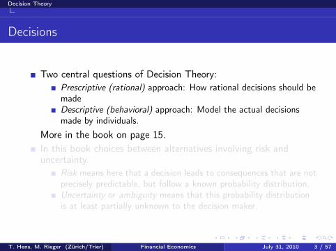
Two central questions of Decision Theory:Prescriptive (rational) approach: How rational decisions should bemadeDescriptive (behavioral) approach: Model the actual decisionsmade by individuals.
More in the book on page 15.In this book choices between alternatives involving risk anduncertainty.
Risk means here that a decision leads to consequences that are notprecisely predictable, but follow a known probability distribution.Uncertainty or ambiguity means that this probability distributionis at least partially unknown to the decision maker.
T. Hens, M. Rieger (Zürich/Trier) Financial Economics July 31, 2010 3 / 57

Decision Theory
Decisions
Two central questions of Decision Theory:Prescriptive (rational) approach: How rational decisions should bemadeDescriptive (behavioral) approach: Model the actual decisionsmade by individuals.
More in the book on page 15.In this book choices between alternatives involving risk anduncertainty.
Risk means here that a decision leads to consequences that are notprecisely predictable, but follow a known probability distribution.Uncertainty or ambiguity means that this probability distributionis at least partially unknown to the decision maker.
T. Hens, M. Rieger (Zürich/Trier) Financial Economics July 31, 2010 3 / 57

Decision Theory
Fundamental Concepts
Preference Relations between Lotteries
A lottery is a given set of states together with their respectiveoutcomes and probabilities.A preference relation is a set of rules that states how we makepairwise decisions between lotteries.Example (see page 16 in the book):
Boom: payoff a1prob1ooooooooo
Recession: payoff a2prob2 OOOOOOOOO
State preference approach:state probability stock bondBoom prob1 as
1 ab1
Recession prob2 as2 ab
2
T. Hens, M. Rieger (Zürich/Trier) Financial Economics July 31, 2010 4 / 57

Decision Theory
Fundamental Concepts
Preference Relations between Lotteries
Lottery approach: add the probabilities of all states where ourasset has the same payoff:
pc =∑
{i=1,...,S | ai=c}
probi .
A preference compares lotteries.A Â B : we prefer lottery A over B .A ∼ B : we are indifferent between A and B .
T. Hens, M. Rieger (Zürich/Trier) Financial Economics July 31, 2010 5 / 57

Decision Theory
Fundamental Concepts
Preference Relation
Definition
A preference relation º on P satisfies the following conditions:(i) It is complete, i.e., for all lotteries A, B ∈ P, either A º B or
B º A or both.(ii) It is transitive, i.e., for all lotteries A, B, C ∈ P with A º B and
B º C we have A º C.More in the book on page 17.
Woody Allen:
Money is better than poverty, if only for financial reasons.
T. Hens, M. Rieger (Zürich/Trier) Financial Economics July 31, 2010 6 / 57

Decision Theory
Fundamental Concepts
State Dominance
Definition
If, for all states s = 1, . . . S, we have aAs ≥ aB
s and there is at least onestate s ∈ {1, . . . , S} with aA
s > aBs , then we say that A state
dominates B. We sometimes write A ºSD B.We say that a preference relation º respects (or is compatible with)state dominance if A ºSD B implies A º B. If º does not respectstate dominance, we say that it violates state dominance.More in the book on page 18.
T. Hens, M. Rieger (Zürich/Trier) Financial Economics July 31, 2010 7 / 57

Decision Theory
Fundamental Concepts
Utility Functional
Definition
Let U be a map that assigns a real number to every lottery. We saythat U is a utility functional for the preference relation º if for everypair of lotteries A and B, we have U(A) ≥ U(B) if and only if A º B.In the case of state independent preference relations, we canunderstand U as a map that assigns a real number to every probabilitymeasure on the set of possible outcomes, i.e., U : P → R.More in the book on page 19.
T. Hens, M. Rieger (Zürich/Trier) Financial Economics July 31, 2010 8 / 57

Decision Theory
Expected Utility Theory
Origins of Expected Utility Theory
The concept of probabilities was developed in the 17th century byPierre de Fermat, Blaise Pascal and Christiaan Huygens, amongothers.Expected value of a lottery A having outcomes xi withprobabilities pi :
E(A) =∑
i
xipi .
T. Hens, M. Rieger (Zürich/Trier) Financial Economics July 31, 2010 9 / 57

Decision Theory
Expected Utility Theory
St. Petersburg Paradox
Daniel Bernoulli:After paying a fixed entrance fee, a fair coin is tossed repeatedly untila “tails” first appears. This ends the game. If the number of times thecoin is tossed until this point is k , you win 2k−1 ducats.
pk = P(“head” on 1st toss) · P(“head” on 2nd toss) · · ·· · ·P(“tail” on k-th toss)
=(1
2
)k.
E(A) =∞∑
k=1
xkpk =∞∑
k=1
2k−1(12
)k
=∞∑
k=1
12
= +∞.
Most people would be willing to pay not more than a couple of ducats.
T. Hens, M. Rieger (Zürich/Trier) Financial Economics July 31, 2010 10 / 57

Decision Theory
Expected Utility Theory
St. Petersburg Lottery
2
1
4
coin toss payoff
Daniel Bernoulli noticed, it is not at all clear why twice the moneyshould always be twice as good.
T. Hens, M. Rieger (Zürich/Trier) Financial Economics July 31, 2010 11 / 57

Decision Theory
Expected Utility Theory
St. Petersburg Paradox
In Bernoulli’s own words:“There is no doubt that a gain of one thousand ducats is moresignificant to the pauper than to a rich man though both gain thesame amount.”Utility function:
utility
money
T. Hens, M. Rieger (Zürich/Trier) Financial Economics July 31, 2010 12 / 57

Decision Theory
Expected Utility Theory
St. Petersburg Paradox
We want to maximize the expected value of the utility, in otherwords, our utility functional becomes
U(p) = E(u) =∑
i
u(xi )pi ,
This resolves the St. Petersburg Paradox.Assume u(x) := ln(x), then
EUT (Lottery) =∑k
u(xk)pk =∑k
ln(2k−1)
(12
)k
= (ln 2)∑k
k − 12k < +∞.
This is caused by the “diminishing marginal utility of money”, seein the book on page 24.
T. Hens, M. Rieger (Zürich/Trier) Financial Economics July 31, 2010 13 / 57

Decision Theory
Expected Utility Theory
Definitions
Definition (Concavity)
We call a function u : R → R concave on the interval (a, b) (whichmight be R) if for all x1, x2 ∈ (a, b) and λ ∈ (0, 1) the followinginequality holds:
λu(x1) + (1− λ)u(x2) ≤ u (λx1 + (1− λ)x2) .
We call u strictly concave if the above inequality is always strict (forx1 6= x2).
Definition (Risk-averse behavior)
We call a person risk-averse if he prefers the expected value of everylottery over the lottery itself.
T. Hens, M. Rieger (Zürich/Trier) Financial Economics July 31, 2010 14 / 57

Decision Theory
Expected Utility Theory
A Strictly Concave Function
x2x1 x0x0 = λx1 + (1− λ)x2
λu(x1) + (1− λ)u(x2)
u(x0)
T. Hens, M. Rieger (Zürich/Trier) Financial Economics July 31, 2010 15 / 57

Decision Theory
Expected Utility Theory
Definitions
Definition (Convexity)
We call a function u : R → R convex on the interval (a, b) if for allx1, x2 ∈ (a, b) and λ ∈ (0, 1) the following inequality holds:
λu(x1) + (1− λ)u(x2) ≥ u(λx1 + (1− λ)x2).
We call u strictly convex if the above inequality is always strict (forx1 6= x2).
Definition (Risk-seeking behavior)
We call a person risk-seeking if he prefers every lottery over itsexpected value.
T. Hens, M. Rieger (Zürich/Trier) Financial Economics July 31, 2010 16 / 57

Decision Theory
Expected Utility Theory
Propositions
Proposition
If u is strictly concave, then a person described by the Expected UtilityTheory with the utility function u is risk-averse. If u is strictly convex,then a person described by the Expected Utility Theory with the utilityfunction u is risk-seeking.
U is fixed only up to monotone transformations and u only up topositive affine transformations:
Proposition
Let λ > 0 and c ∈ R. If u is a utility function that corresponds to thepreference relation º, i.e., A º B implies U(A) ≥ U(B), thenv(x) := λu(x) + c is also a utility function corresponding to º.
More in the book on page 27.T. Hens, M. Rieger (Zürich/Trier) Financial Economics July 31, 2010 17 / 57

Decision Theory
Expected Utility Theory
Axiomatic Definition
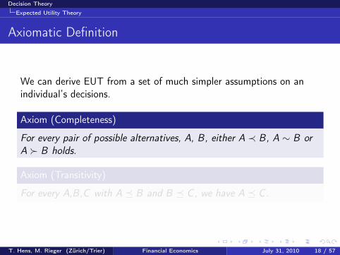
We can derive EUT from a set of much simpler assumptions on anindividual’s decisions.
Axiom (Completeness)
For every pair of possible alternatives, A, B, either A ≺ B, A ∼ B orA Â B holds.
Axiom (Transitivity)
For every A,B,C with A ¹ B and B ¹ C, we have A ¹ C.
T. Hens, M. Rieger (Zürich/Trier) Financial Economics July 31, 2010 18 / 57
Decision Theory
Expected Utility Theory
Axiomatic Definition
We can derive EUT from a set of much simpler assumptions on anindividual’s decisions.
Axiom (Completeness)
For every pair of possible alternatives, A, B, either A ≺ B, A ∼ B orA Â B holds.
Axiom (Transitivity)
For every A,B,C with A ¹ B and B ¹ C, we have A ¹ C.
T. Hens, M. Rieger (Zürich/Trier) Financial Economics July 31, 2010 18 / 57

Decision Theory
Expected Utility Theory
The Cycle of the “Lucky Hans”, Violating Transitivity
Gold
Horse
Cow
PigGoose
Nothing
Grindstone
T. Hens, M. Rieger (Zürich/Trier) Financial Economics July 31, 2010 19 / 57

Decision Theory
Expected Utility Theory
Axiomatic Definition
Definition
Let A and B be lotteries and λ ∈ [0, 1], then λA+ (1− λ)B denotes anew combined lottery where with probability λ the lottery A is played,and with probability 1− λ the lottery B is played.
An example can be found in the book on page 31.
Axiom (Independence)
Let A and B be two lotteries with A Â B, and let λ ∈ (0, 1] then forany lottery C, it must hold
λA + (1− λ)C Â λB + (1− λ)C .
T. Hens, M. Rieger (Zürich/Trier) Financial Economics July 31, 2010 20 / 57

Decision Theory
Expected Utility Theory
Axiomatic Definition
Axiom (Continuity)
Let A,B,C be lotteries with A º B º C then there exists aprobability p such that B ∼ pA + (1− p)C.
Theorem (Expected Utility Theory)
A preference relation that satisfies the Completeness Axiom 1, theTransitivity Axiom 2, the Independence Axiom 3 and the ContinuityAxiom 4, can be represented by an EUT functional. EUT alwayssatisfies these axioms.
The proof can be found in the book on page 33.
T. Hens, M. Rieger (Zürich/Trier) Financial Economics July 31, 2010 21 / 57
Decision Theory
Expected Utility Theory
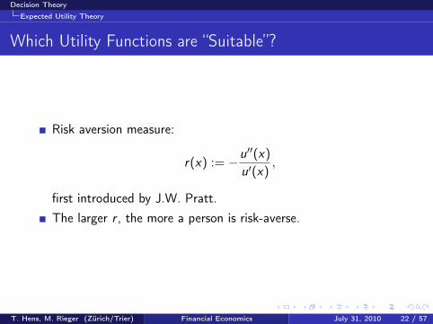
Which Utility Functions are “Suitable”?
Risk aversion measure:
r(x) := −u′′(x)
u′(x),
first introduced by J.W. Pratt.The larger r , the more a person is risk-averse.
T. Hens, M. Rieger (Zürich/Trier) Financial Economics July 31, 2010 22 / 57

Decision Theory
Expected Utility Theory
Which Utility Functions are “Suitable”?
Proposition
Let p be the outcome distribution of a lottery with E(p) = 0, in otherwords, p is a fair bet. Let w be the wealth level of the person, then,neglecting higher order terms in r(w) and p,
EUT (w + p) = u(w − 1
2var(p)r(w)
),
where var(p) denotes the variance of p. We could say that the “riskpremium”, i.e., the amount the person is willing to pay for aninsurance against a fair bet, is proportional to r(w).
The proof can be found in the book on page 37.
T. Hens, M. Rieger (Zürich/Trier) Financial Economics July 31, 2010 23 / 57
Decision Theory
Expected Utility Theory
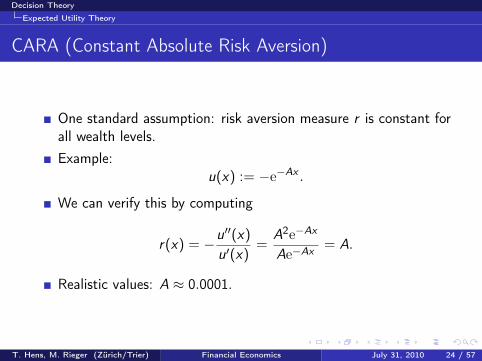
CARA (Constant Absolute Risk Aversion)
One standard assumption: risk aversion measure r is constant forall wealth levels.Example:
u(x) := −e−Ax .
We can verify this by computing
r(x) = −u′′(x)
u′(x)=
A2e−Ax
Ae−Ax = A.
Realistic values: A ≈ 0.0001.
T. Hens, M. Rieger (Zürich/Trier) Financial Economics July 31, 2010 24 / 57

Decision Theory
Expected Utility Theory
CRRA (Constant Relative Risk Aversion)
Another standard approach: r(x) should be proportional to x .Relative risk aversion:
rr(x) := xr(x) = −x u′′(x)
u′(x)
is constant for all x .Examples:
u(x) :=xR
R, where R < 1, R 6= 0,
u(x) := ln x .
Typical values for R are between −1 and −3.
T. Hens, M. Rieger (Zürich/Trier) Financial Economics July 31, 2010 25 / 57

Decision Theory
Expected Utility Theory
HARA (Hyperbolic Absolute Risk Aversion)
Generalization of the classes of utility functions.All functions where the reciprocal of absolute risk aversion,T := 1/r(x), is an affine function of x .
Proposition
A function u : R → R is HARA if and only if it is an affinetransformation of one of these functions:
v1(x) := ln(x + a), v2(x) := −ae−x/a, v3(x) :=(a + bx)(b−1)/b
b − 1,
where a and b are arbitrary constants (b 6∈ {0, 1} for v3). If we defineb := 1 for v1 and b := 0 for v2, we have in all three cases T = a + bx.
T. Hens, M. Rieger (Zürich/Trier) Financial Economics July 31, 2010 26 / 57

Decision Theory
Expected Utility Theory
Classes of Utility Functions
Class of utilities Definition ARA r(x) RRA rr(x) Special propertiesLogarithmic ln(x + c), c ≥ 0 decr. const. “Bernoulli utility”
Power 1α
xα, α 6= 0 decr. const. risk-averse if α < 1,bounded if α < 0
Quadratic x − αx2, α > 0 incr. incr. bounded, monotoneonly up to x = (2α)−1
Exponential −e−αx , α > 0 const. incr. bounded
“Super St. Petersburg Paradox”, see in the book on page 41.
Theorem (St. Petersburg Lottery)
Let p be the outcome distribution of a lottery. Let u : R → R be autility function.(i) If u is bounded, then EUT (p) :=
∫u(x) dp < ∞.
(ii) Assume that E(p) < ∞. If u is asymptotically concave, i.e.,there is a C > 0 such that u is concave on the interval [C , +∞),then EUT (p) < ∞.
T. Hens, M. Rieger (Zürich/Trier) Financial Economics July 31, 2010 27 / 57

Decision Theory
Expected Utility Theory
Measuring the Utility Function
Midpoint certainty equivalent method.A subject is asked to state a monetary equivalent to a lotterywith two outcomes.Each with probability 1/2.Such a monetary equivalent is called a Certainty Equivalent (CE).Set u(x0) := 0 and u(x1) := 1, then u(CE ) = 0.5.Set x0.5 := CE and iterate this method by comparing a lotterywith the outcomes x0 and x0.5 and probabilities 1/2 each etc.An example can be found in the book on page 44.
T. Hens, M. Rieger (Zürich/Trier) Financial Economics July 31, 2010 28 / 57

Decision Theory
Mean-Variance Theory
Definition and Fundamental Properties
Introduced in 1952 by MarkowitzKey idea: measure the risk of an asset by only one parameter, thevariance σ.
Definition (Mean-Variance approach)
A mean-variance utility function u is a utility function u : R×R+ → Rwhich corresponds to a utility functional U : P → R that only dependson the mean and the variance of a probability measure p, i.e.,U(p) = u(E(p), var(p)).
Definition
A mean-variance utility function u : R×R+ → R is called monotone ifu(µ, σ) ≥ u(ν, σ) for all µ, ν, σ with µ > ν. It is called strictlymonotone if even u(µ, σ) > u(ν, σ).
T. Hens, M. Rieger (Zürich/Trier) Financial Economics July 31, 2010 29 / 57

Decision Theory
Mean-Variance Theory
Definition and Fundamental Properties
Definition
A mean-variance utility function u : R× R+ → R is calledvariance-averse if u(µ, σ) ≥ u(µ, τ) for all µ, τ, σ with τ > σ. It iscalled strictly variance-averse if u(µ, σ) > u(µ, τ) for all µ, τ, σ withτ > σ.
Remark
Let u be a mean-variance function. Then the preference induced by uis risk-averse if and only if u(µ, σ) < u(µ, 0) for all µ, σ. Thepreference is risk-seeking if and only if u(µ, σ) > u(µ, 0).
Example:u1(µ, σ) := µ− σ2.
T. Hens, M. Rieger (Zürich/Trier) Financial Economics July 31, 2010 30 / 57
Decision Theory
Mean-Variance Theory
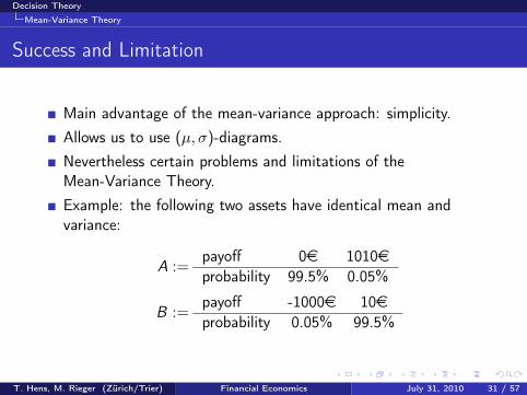
Success and Limitation
Main advantage of the mean-variance approach: simplicity.Allows us to use (µ, σ)-diagrams.Nevertheless certain problems and limitations of theMean-Variance Theory.Example: the following two assets have identical mean andvariance:
A :=payoff 0e 1010eprobability 99.5% 0.05%
B :=payoff -1000e 10eprobability 0.05% 99.5%
T. Hens, M. Rieger (Zürich/Trier) Financial Economics July 31, 2010 31 / 57

Decision Theory
Mean-Variance Theory
Success and Limitation
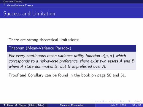
There are strong theoretical limitations:
Theorem (Mean-Variance Paradox)
For every continuous mean-variance utility function u(µ, σ) whichcorresponds to a risk-averse preference, there exist two assets A and Bwhere A state dominates B, but B is preferred over A.
Proof and Corollary can be found in the book on page 50 and 51.
T. Hens, M. Rieger (Zürich/Trier) Financial Economics July 31, 2010 32 / 57
Decision Theory
Mean-Variance Theory
Success and Limitation
There are strong theoretical limitations:
Theorem (Mean-Variance Paradox)
For every continuous mean-variance utility function u(µ, σ) whichcorresponds to a risk-averse preference, there exist two assets A and Bwhere A state dominates B, but B is preferred over A.
Proof and Corollary can be found in the book on page 50 and 51.
T. Hens, M. Rieger (Zürich/Trier) Financial Economics July 31, 2010 32 / 57

Decision Theory
Prospect Theory
Prospect Theory
How do people really decide?As if they were maximizing their expected utility?Or as if they were following the mean-variance approach?
T. Hens, M. Rieger (Zürich/Trier) Financial Economics July 31, 2010 33 / 57

Decision Theory
Prospect Theory
Example: Allais Paradox
Consider four lotteries A, B, C and D.In each lottery a random number is drawn from the set{1, 2, . . . , 100} where each number occurs with the sameprobability of 1%.The lotteries assign outcomes to every of these 100 possiblenumbers (states).The test persons are asked to decide between the two lotteries Aand B and then between C and D. Most people prefer B over Aand C over D.This behavior is not rational and violates the IndependenceAxiom.
T. Hens, M. Rieger (Zürich/Trier) Financial Economics July 31, 2010 34 / 57

Decision Theory
Prospect Theory
The four lotteries of Allais’ Paradox
Lottery AState 1–33 34–99 100Outcome 2500 2400 0
Lottery BState 1–100Outcome 2400
Lottery CState 1–33 34–100Outcome 2500 0
Lottery DState 1–33 34–99 100Outcome 2400 0 2400
T. Hens, M. Rieger (Zürich/Trier) Financial Economics July 31, 2010 35 / 57

Decision Theory
Prospect Theory
Observed Facts
People tend to buy insurances (risk-averse behavior) and takepart in lotteries (risk-seeking behavior) at the same time.People are usually risk-averse even for small-stake gambles andlarge initial wealth. This would predict a degree on risk aversionfor high-stake gambles that is far away from standard behavior.Does this mean, that the “homo economicus” is dead and that allmodels of humans as rational deciders are obsolete?Is “science at a loss” when it comes to people’s decisions?The “homo economicus” is still a central concept, and there aremodifications that describe human decisions.
T. Hens, M. Rieger (Zürich/Trier) Financial Economics July 31, 2010 36 / 57
Decision Theory
Prospect Theory
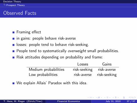
Observed Facts
Framing effectin gains: people behave risk-averselosses: people tend to behave risk-seeking.People tend to systematically overweight small probabilities.Risk attitudes depending on probability and frame:
Losses GainsMedium probabilities risk-seeking risk-averseLow probabilities risk-averse risk-seeking
We explain Allais’ Paradox with this idea.
T. Hens, M. Rieger (Zürich/Trier) Financial Economics July 31, 2010 37 / 57

Decision Theory
Prospect Theory
Original Prospect Theory
Kahneman and TverskyInstead of the final wealth we consider the gain and loss (framingeffect) instead of the real probabilities we consider weightedprobabilitiesSubjective utility:
PT (A) :=n∑
i=1
v(xi )w(pi ),
where v : R → R is the value function, defined on losses andgains. w : [0, 1] → [0, 1] is the probability weighting function.
T. Hens, M. Rieger (Zürich/Trier) Financial Economics July 31, 2010 38 / 57
Decision Theory
Prospect Theory
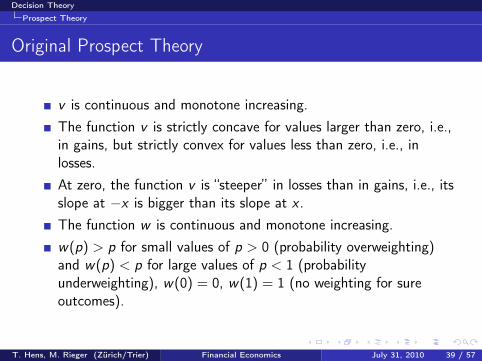
Original Prospect Theory
v is continuous and monotone increasing.The function v is strictly concave for values larger than zero, i.e.,in gains, but strictly convex for values less than zero, i.e., inlosses.At zero, the function v is “steeper” in losses than in gains, i.e., itsslope at −x is bigger than its slope at x .The function w is continuous and monotone increasing.w(p) > p for small values of p > 0 (probability overweighting)and w(p) < p for large values of p < 1 (probabilityunderweighting), w(0) = 0, w(1) = 1 (no weighting for sureoutcomes).
T. Hens, M. Rieger (Zürich/Trier) Financial Economics July 31, 2010 39 / 57

Decision Theory
Prospect Theory
Original Prospect Theory
relativereturn
value
1
1
prob.
weighted prob.
T. Hens, M. Rieger (Zürich/Trier) Financial Economics July 31, 2010 40 / 57

Decision Theory
Prospect Theory
Original Prospect Theory
If we have many events, all of them will probably be overweightedand the sum of the weighted probabilities will be large.Alternative formulation of Prospect Theory that fixes the problem:
PT (A) =
∑ni=1 v(xi )w(pi )∑n
i=1 w(pi ).
More about this and the four-fold pattern in the book on page 58.
T. Hens, M. Rieger (Zürich/Trier) Financial Economics July 31, 2010 41 / 57

Decision Theory
Prospect Theory
Original Prospect Theory
Definition (Stochastic dominance)
A lottery A is stochastically dominant over a lottery B if, for everypayoff x, the probability to obtain more than x is larger or equal for Athan for B and there is at least some payoff x such that thisprobability is strictly larger.
An example can be found in the book on page 59.
PT violates stochastic dominance.Another limitation: PT can only be applied for finitely manyoutcomes.In finance, however, we are interested ininfinitely many outcomes.
T. Hens, M. Rieger (Zürich/Trier) Financial Economics July 31, 2010 42 / 57

Decision Theory
Prospect Theory
Cumulative Prospect Theory
Key idea: Replace the probabilities by differences of cumulativeprobabilities.
Definition (Cumulative Prospect Theory)
For a lottery A with n outcomes x1, . . . , xn and the probabilitiesp1, . . . , pn where x1 < x2 < · · · < xn and
∑ni=1 pi = 1 we define
CPT (A) :=n∑
i=1
(w(Fi )− w(Fi−1)) v(xi ), (1)
where F0 := 0 and Fi :=∑i
j=1 pj for i = 1, . . . , n.
How this formula is connected to Prospect Theory is written in thebook on page 60.
T. Hens, M. Rieger (Zürich/Trier) Financial Economics July 31, 2010 43 / 57
Decision Theory
Prospect Theory
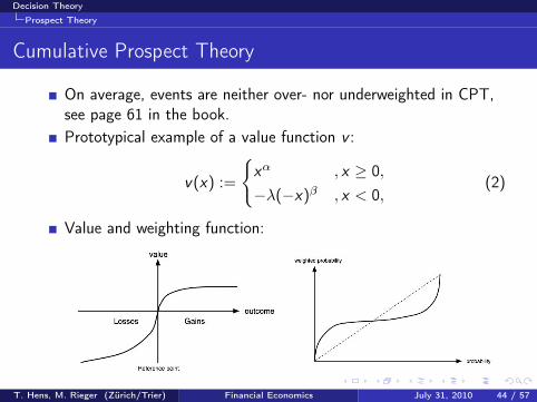
Cumulative Prospect Theory
On average, events are neither over- nor underweighted in CPT,see page 61 in the book.Prototypical example of a value function v :
v(x) :=
{xα , x ≥ 0,−λ(−x)β , x < 0,
(2)
Value and weighting function:
T. Hens, M. Rieger (Zürich/Trier) Financial Economics July 31, 2010 44 / 57

Decision Theory
Prospect Theory
Cumulative Prospect Theory
Probability weighting function w :
w(p) :=pγ
(pγ + (1− p)γ)1/γ,
Experimental values:
Study Estimate Estimatefor α,β for γ, δ
Tversky and Kahnemangains: 0.88 0.61losses: 0.88 0.69
Camerer and Ho 0.37 0.56Tversky and Fox 0.88 0.69Wu and Gonzalez
gains: 0.52 20.71Abdellaoui
gains: 0.89 0.60losses: 0.92 0.70
Bleichrodt and Pinto 0.77 0.67/0.55Kilka and Weber 0.76-1.00 0.30-0.51
T. Hens, M. Rieger (Zürich/Trier) Financial Economics July 31, 2010 45 / 57

Decision Theory
Prospect Theory
Cumulative Prospect Theory
Extend CPT to arbitrary lotteries.we can describe lotteries by probability measures, seeAppendix A.4 for details.
Definition
Let p be an arbitrary probability measure, then the generalized form ofCPT reads as
CPT (p) :=
∫ +∞
−∞v(x)
(ddt
w(F (t))|t=x
)dx , (3)
where
F (t) :=
∫ t
−∞dp.
T. Hens, M. Rieger (Zürich/Trier) Financial Economics July 31, 2010 46 / 57

Decision Theory
Prospect Theory
Cumulative Prospect Theory
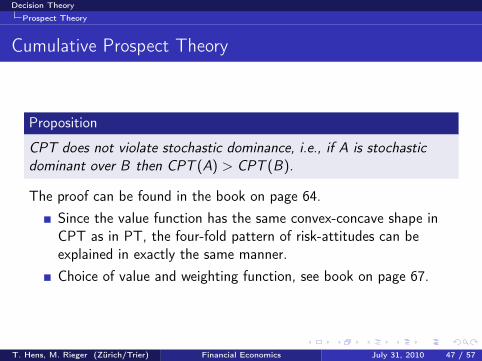
Proposition
CPT does not violate stochastic dominance, i.e., if A is stochasticdominant over B then CPT (A) > CPT (B).
The proof can be found in the book on page 64.Since the value function has the same convex-concave shape inCPT as in PT, the four-fold pattern of risk-attitudes can beexplained in exactly the same manner.Choice of value and weighting function, see book on page 67.
T. Hens, M. Rieger (Zürich/Trier) Financial Economics July 31, 2010 47 / 57
Decision Theory
Prospect Theory
Cumulative Prospect Theory
Proposition
CPT does not violate stochastic dominance, i.e., if A is stochasticdominant over B then CPT (A) > CPT (B).
The proof can be found in the book on page 64.Since the value function has the same convex-concave shape inCPT as in PT, the four-fold pattern of risk-attitudes can beexplained in exactly the same manner.Choice of value and weighting function, see book on page 67.
T. Hens, M. Rieger (Zürich/Trier) Financial Economics July 31, 2010 47 / 57

Decision Theory
Connecting EUT, Mean-Variance Theory and PT
EUT, Mean-Variance Theory and CPT
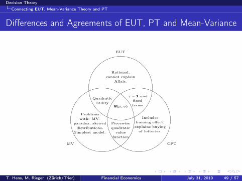
EUT is the “rational benchmark”. We will use it as a reference ofrational behavior and as a prescriptive theory when we want tofind an objectively optimal decision.Mean-Variance Theory is the “pragmatic solution”. The theory iswidely used in finance.CPT model “real life behavior”. We will use it to describebehavior patterns of investors.
T. Hens, M. Rieger (Zürich/Trier) Financial Economics July 31, 2010 48 / 57
Decision Theory
Connecting EUT, Mean-Variance Theory and PT
Differences and Agreements of EUT, PT and Mean-Variance
utility
γ = 1 andfixedframe
cannot explainAllais.
Quadratic
MV
framing effect,explains buyingof lotteries.
paradox, skewedwith: MV-
CPT
Includes
EUT
Simplest model.
Problems
distributions.Piecewisequadraticvalue
N(µ, σ)
Rational,
function
T. Hens, M. Rieger (Zürich/Trier) Financial Economics July 31, 2010 49 / 57

Decision Theory
Ambiguity and Uncertainty?
Ambiguity and Uncertainty
Often probabilities are known. We call this ambiguity oruncertainty.Example:There is an urn with 300 balls. 100 of them are red, 200 are blueor green. You can pick red or blue and then take one ball (blindly,of course). If it is of the color you picked, you win 100e, else youdon’t win anything. Which color do you choose?Most people choose red.Example:Same situation, you pick again a color (either red or blue) andthen take a ball. This time, if the ball is not of the color youpicked, you win 100e, else you don’t win anything. Which colordo you choose?Most people indeed pick red.
T. Hens, M. Rieger (Zürich/Trier) Financial Economics July 31, 2010 50 / 57

Decision Theory
Ambiguity and Uncertainty?
Ambiguity and Uncertainty
People go both times for the “sure” option, the option where theyknow their probabilities to win.Uncertainty-aversity, see book on page 81.People are often not very knowledgeable about the chances andrisks of financial investments.This explains why many people invest into very few stocks (thatthey are familiar with) or even only into the stock of their owncompany (even if their company is not performing well).
T. Hens, M. Rieger (Zürich/Trier) Financial Economics July 31, 2010 51 / 57

Decision Theory
Time Discounting
Time Discounting
Original utility:u(t) = u(0)e−δt ,
Classical time discounting leads to a time-consistent preference.More details in the book on page 82.Hyperbolic discounting:
u(t) =u(0)1 + δt
Quasi-hyperbolic discounting:
u(t) =
{u(0) , for t = 0,
11+βu(0)e−δt , for t > 0, where β > 0.
An example can be found in the book on page 84.
T. Hens, M. Rieger (Zürich/Trier) Financial Economics July 31, 2010 52 / 57

Decision Theory
Time Discounting
Rational versus Hyperbolic Time Discounting
time t
discounted utility
e−δt
u(t) =u(0)
1 + δt
T. Hens, M. Rieger (Zürich/Trier) Financial Economics July 31, 2010 53 / 57

References
References
T. Hens, M. Rieger (Zürich/Trier) Financial Economics July 31, 2010 54 / 57

References
References I
Abdeallaoui, M. (2000).Parameter-free elicitation of utilities and probability weightingfunctions.Management Science, 46:1497–1512.
Bleichrodt, H. and Pinto, J. L. (2000).A parameter-free elicitation of the probability weighting functionin medical decision analysis.Management science, 46:1485–1496.
Camerer, C. and Ho, T.-H. (1994).Violations of the betweenness axiom and nonlinearity inprobability.Journal of Risk and Uncertainty, 8:167–196.
T. Hens, M. Rieger (Zürich/Trier) Financial Economics July 31, 2010 55 / 57

References
References II
Kilka, M. and Weber, M. (2001).What determines the shape of the proability weighting functionunder uncertainty?Management Science, 47(12):1712–1726.
Tversky, A. and Fox, C. R. (1995).Weighing risk and uncertainty.Psychological Review, 102(2):269–283.
Tversky, A. and Kahneman, D. (1992).Advances in Prospect Theory: Cumulative representation ofuncertainty.Journal of Risk and Uncertainty, 5:297–323.
T. Hens, M. Rieger (Zürich/Trier) Financial Economics July 31, 2010 56 / 57

References
References III
Wu, G. and Gonzalez, R. (1996).Curvature of the probability weighting function.Management Science, 42:1676–1690.
T. Hens, M. Rieger (Zürich/Trier) Financial Economics July 31, 2010 57 / 57