FINANCIAL CONSTRAINTS, THE USER COST OF CAPITAL AND CORPORATE INVESTMENT IN AUSTRALIA

Gianni La Cava

Research Discussion Paper 2005-12

December 2005

Economic Analysis Reserve Bank of Australia

The author would like to thank Luci Ellis, James Holloway, Christopher Kent, Tony Richards, Geoffrey Shuetrim, James Vickery, seminar participants at the Reserve Bank of Australia and especially Alex Heath for helpful comments and discussion. The views expressed in this paper are those of the author and do not necessarily reflect the views of the Reserve Bank of Australia.

Abstract

This paper examines the factors that drive corporate investment in Australia using a panel of listed companies covering the period from 1990 to 2004. Real sales growth is found to be a significant determinant of corporate investment. The user cost of capital, which incorporates both debt and equity financing costs, also appears to be an important determinant.

The paper also explores the effects of cash flow on investment, allowing for the possibility that the availability of internal funding could significantly affect the investment of financially constrained firms. Cash flow is found to affect investment, though the effects appear more complicated than previously reported in empirical research using Australian data. One innovation of this study is that it distinguishes financially distressed firms from financially constrained firms. The presence of financially distressed firms appears to bias downwards the sensitivity of investment to cash flow. Once separate account has been taken of firms experiencing financial distress, and in contrast to theory, cash flow is found to matter for the investment of both financially constrained and unconstrained firms. Interestingly, the estimated degree of sensitivity appears to be roughly the same for both groups.

JEL Classification Numbers: E22, E44, E52

Keywords: investment, user cost of capital, panel data

i

Table of Contents

1. Introduction 1

2. Theory 3

2.1 Definition of Financial Constraints 3

2.2 Measurement of Financial Constraints 7

2.3 Financially Constrained versus Financially Distressed Firms 9

3. Data 11

3.1 Sample Selection 11

3.2 Variables in the Model 13

3.3 Sample Characteristics and Comparisons to Aggregate Data 16

4. Modelling Strategy and Results 19

4.1 Estimation Method 19

4.2 Other Modelling Issues 23

4.3 Results 24

4.4 The Effect of Financial Constraints and Financial Distress 28

5. Conclusion 30

Appendix A: Variable Definitions, Sources and Summary Statistics 31

Appendix B: Measurement Issues 34

Appendix C: Comparisons with Earlier Australian Studies 36

References 37

ii

FINANCIAL CONSTRAINTS, THE USER COST OF CAPITAL AND CORPORATE INVESTMENT IN AUSTRALIA

Gianni La Cava

1. Introduction

The pace and pattern of business investment in fixed capital are central to our understanding of economic activity. Business investment is one of the key determinants of an economy’s long-term growth rate and also plays a pivotal role in explaining business cycle fluctuations. And yet, despite extensive empirical research, it has been hard to clearly identify a role for some of the factors that are believed to drive capital spending.

This at least partly reflects an ‘aggregation problem’ – the drivers of capital spending can vary a lot in terms of both their magnitude and timing across different industries and markets. To circumvent this problem, this paper uses panel data on individual firms to model investment spending in Australia. The use of panel data has several advantages over aggregate data. First, by introducing cross-sectional variation, panel data can help to minimise the simultaneity problem that often occurs in macro studies of investment. For example, policy-makers, in anticipation of future excess demand, might raise interest rates at the same time that investment demand increases. All else equal, this would result in a positive relationship between interest rates and investment, in contrast to the predictions of neoclassical theory. Second, cross-sectional variation allows the relationships between investment and its determinants to be measured using fairly short time series. Finally, panel-data analysis allows us to determine whether changes in financing costs are more important for certain types of firms or industries. By recognising firm and industry heterogeneity we can better understand the monetary policy transmission mechanism.

This paper estimates an error correction model (ECM) of corporate investment. The ECM framework has the relative advantage of modelling both the short-run dynamics and long-run determinants of investment, such as real sales growth and the user cost of capital. To the best of my knowledge, this is the first time this has

2

been done using Australian panel data. As well as long-run determinants such as real sales growth and the user cost of capital, a vast literature suggests that financial factors are also important in explaining short-run fluctuations in investment.1 Transaction costs and/or information asymmetries induce a cost premium that makes external finance an imperfect substitute for internal finance (Jensen and Meckling 1976; Stiglitz and Weiss 1981; Myers and Majluf 1984). When capital markets are imperfect, some firms may be ‘financially constrained’ in the sense that they are unable to raise enough external funds to meet their desired level of investment spending. If this is the case, in the short run, the level of internal funding could significantly affect investment.

Including financial factors as short-run determinants is also important for understanding the monetary policy transmission process: if capital markets are imperfect and firms face additional costs of raising external finance, then interest rate changes may affect capital spending by influencing the amount of funds available. This effect can occur over and above the direct effect of interest rate changes on the relative price of capital goods and hence, business investment. It has become common practice to refer to these two channels of monetary policy as the ‘credit’ and ‘interest rate’ channels.

A finding that internal funding has a significant effect on firm-level investment can be taken as evidence of financial constraints. In principle, financially constrained firms should display greater sensitivity of investment to cash flow than unconstrained firms. However, internal funding could be relevant for investment because it also provides information about future investment opportunities (Bond et al 2004). To control for this, I also estimate a Q-type model in which the ratio of the market to book value of a firm’s equity (Q) plays a key role in explaining its investment. This is the approach used in earlier Australian studies (Shuetrim, Lowe and Morling 1993; Mills, Morling and Tease 1994; Chapman, Junor and Stegman 1996).

The paper is organised as follows. Section 2 begins with a discussion of the role of financial constraints in influencing investment. Section 3 discusses the panel data used and compares measures of investment, sales, the user cost of capital and cash

1 For surveys of the literature, see Blundell, Bond and Meghir (1992), Chirinko (1993),

Schiantarelli (1996), Hubbard (1998) and Bond and Van Reenen (2003).

3

flow at both the micro and macro levels. A model is then estimated in Section 4 to examine the determinants of corporate investment in Australia. This section also outlines the key results and makes some comparisons with the results of other international studies. Section 5 concludes.

2. Theory

2.1 Definition of Financial Constraints

Under the perfect capital market assumption, the Modigliani-Miller theorem suggests that a firm’s capital structure is irrelevant to its value. This implies that external finance (new debt and/or equity issues) and internal finance (retained earnings) are perfect substitutes and a firm’s investment and financing decisions are independent of each other. The availability of internal funding does not matter for investment, so the price at which firms can obtain funds becomes the only financial consideration in determining the level of investment.

However, there are a number of reasons why capital markets are not perfect. In particular, taxes, transaction costs and information asymmetries (between lenders and borrowers and/or between managers and shareholders) can make external sources of finance more costly than internal finance. If markets are characterised by imperfect information, investment finance may only be available on less favourable terms in external capital markets, or may not be available at all. This implies that the investment spending of some firms may be constrained by a shortage of internal funds. As a result, the level of internal funding could be an important determinant of investment empirically. To understand this concept of financial constraints it is useful to consider Figure 1.2

2 The discussion and graphical analysis are adopted from Bond and Meghir (1994).

4

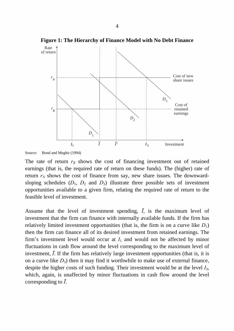
Figure 1: The Hierarchy of Finance Model with No Debt Finance

D1

Rateof return

Cost of newshare issues

Cost ofretainedearnings

Investment

D2

D3

I

rN

rR

I1 I3′I Source: Bond and Meghir (1994)

The rate of return rR shows the cost of financing investment out of retained earnings (that is, the required rate of return on these funds). The (higher) rate of return rN shows the cost of finance from say, new share issues. The downward-sloping schedules (D1, D2 and D3) illustrate three possible sets of investment opportunities available to a given firm, relating the required rate of return to the feasible level of investment.

Assume that the level of investment spending, Ī, is the maximum level of investment that the firm can finance with internally available funds. If the firm has relatively limited investment opportunities (that is, the firm is on a curve like D1) then the firm can finance all of its desired investment from retained earnings. The firm’s investment level would occur at I1 and would not be affected by minor fluctuations in cash flow around the level corresponding to the maximum level of investment, Ī. If the firm has relatively large investment opportunities (that is, it is on a curve like D3) then it may find it worthwhile to make use of external finance, despite the higher costs of such funding. Their investment would be at the level I3, which, again, is unaffected by minor fluctuations in cash flow around the level corresponding to Ī.

5

Consider the intermediate case, illustrated by the curve D2, where financial constraints (in the form of limited retained earnings) affect the investment spending of firms. Such firms have sufficiently profitable investment opportunities that they exhaust all their internal funds. However, their remaining projects are not so attractive that they can cover the higher rate of return required by external funding sources. The investment spending of such constrained firms is limited to the level that can be financed from retained earnings.

A ‘financially constrained’ firm can be thought of as a firm whose investment spending would rise (fall) if its retained earnings increased (decreased). For example, a rise in retained earnings would shift the maximum level of investment that can be financed internally, say from Ī to Ī´, so that there would be a commensurate increase in the investment of constrained firms.

Including debt finance complicates the story but the implications for investment remain basically the same.3 If the cost of debt finance rises with the amount raised (commensurate with the higher risk of default), the supply schedule for external funds has a kink in it at the investment level, Ī (Figure 2). For firms in Regimes 1 and 3 the situation is basically unchanged, although Regime 3 firms can now finance investment through both debt and equity issues.

On the other hand, firms in Regime 2 are no longer constrained to the level of investment given by Ī. They can finance higher investment by borrowing to the extent that they find it worthwhile to bear the increasing cost. In this case, their investment is determined by the rising cost of debt, giving the level I2. However, they are still financially constrained since an increase in cash flow would allow levels of investment above Ī to be financed at lower levels of borrowing. This reduces the effective cost of debt at each level of investment, resulting in higher investment at I2´. As before, the investment of firms in this position is limited by the availability of internal finance, even though they have access to external finance.

3 Debt finance is typically less costly than equity finance since debt holders will have priority

over equity holders in the event that the firm goes bankrupt.

6

Figure 2: Hierarchy of Finance Model with Debt Finance

D1

Rateof return

Cost of newshare issues

Cost ofretainedearnings

Investment

D2

D3

I

rN

rR

I1 I3′I I2 ′I2 Source: Bond and Meghir (1994)

Some of the channels of monetary transmission can also be distinguished using Figure 2. Take, for instance, the case of a tightening of monetary policy. This will increase the required rate of return on retained earnings, rR, and shift up the supply schedule for external funds. This rise in the relative cost of capital will reduce the investment of all firms, regardless of whether they are constrained or not. This effect is commonly referred to as the interest-rate channel of monetary policy.

However, the rate rise will also increase the gradient of the loan supply schedule. This happens either because the rate rise increases the net interest payments (reduces the cash flow) of leveraged firms, or because it reduces the discounted value of assets used as collateral.4 In either case, the firm’s risk premium (and hence effective cost of borrowing) should rise. This, in turn, will restrict the amount of funding available, thereby affecting the investment behaviour of financially constrained firms – the credit channel of monetary policy.

4 The rate rise will only directly affect the cash flow of leveraged firms with outstanding

floating-rate debt. The example also does not consider that firms may hedge against interest rate risk, which could partly dilute the effect of the credit channel on investment.

7

This theory implies that it may be necessary to include a measure of internal funding (such as cash flow) in an estimated model of investment spending. However, it is important to note that finding a significant role for internal funding measures in explaining investment does not necessarily imply that some firms are financially constrained. If the estimated model does not adequately control for investment opportunities then internal funding could be significant because it provides information about future profitability and hence investment. A structural Q-type model may alleviate this problem and this model is discussed in Section 4.5

2.2 Measurement of Financial Constraints

To assess the effects of financial constraints on corporate investment requires financially constrained firms to be identified. Unfortunately, there is no consensus as to the best method of measuring (unobservable) financial constraints. Studies have tried to identify financially constrained firms on the basis of dividend payout ratios, firm size, age, industrial group membership, the nature of the bank-firm relationship, the presence of bond ratings and the degree of ownership concentration (Schiantarelli 1996).

This paper uses reductions in dividend payments as an indication of financial constraint (Cleary 1999; Siegfried 2000). Firms that are unconstrained have no incentive to cut dividend payments while constrained firms can cut dividends to free up internal funds for profitable investment projects. Therefore, firms are classified as financially constrained if they have cut nominal dividend payments in either the current or previous period. This has the advantage over more ad hoc identification schemes since the decision to cut dividends is part of the firm’s optimisation problem (Schiantarelli 1996). By using a dummy for periods in which a firm makes a dividend cut, this classification scheme also allows firms to switch between constrained and unconstrained ‘regimes’ over the sample period.

5 However, there remains the possibility that internal funding is significant because managers

use free cash flow (cash flow remaining after investment in profitable projects has been realised) to over-invest. The ‘free cash flow hypothesis’ suggests that if managers engage in such sub-optimal investment policies, the Q model is also not an appropriate description of firm investment behaviour (Jensen 1986). While this remains a possibility, free cash flow is difficult to observe and testing this hypothesis is beyond the scope of this paper.

8

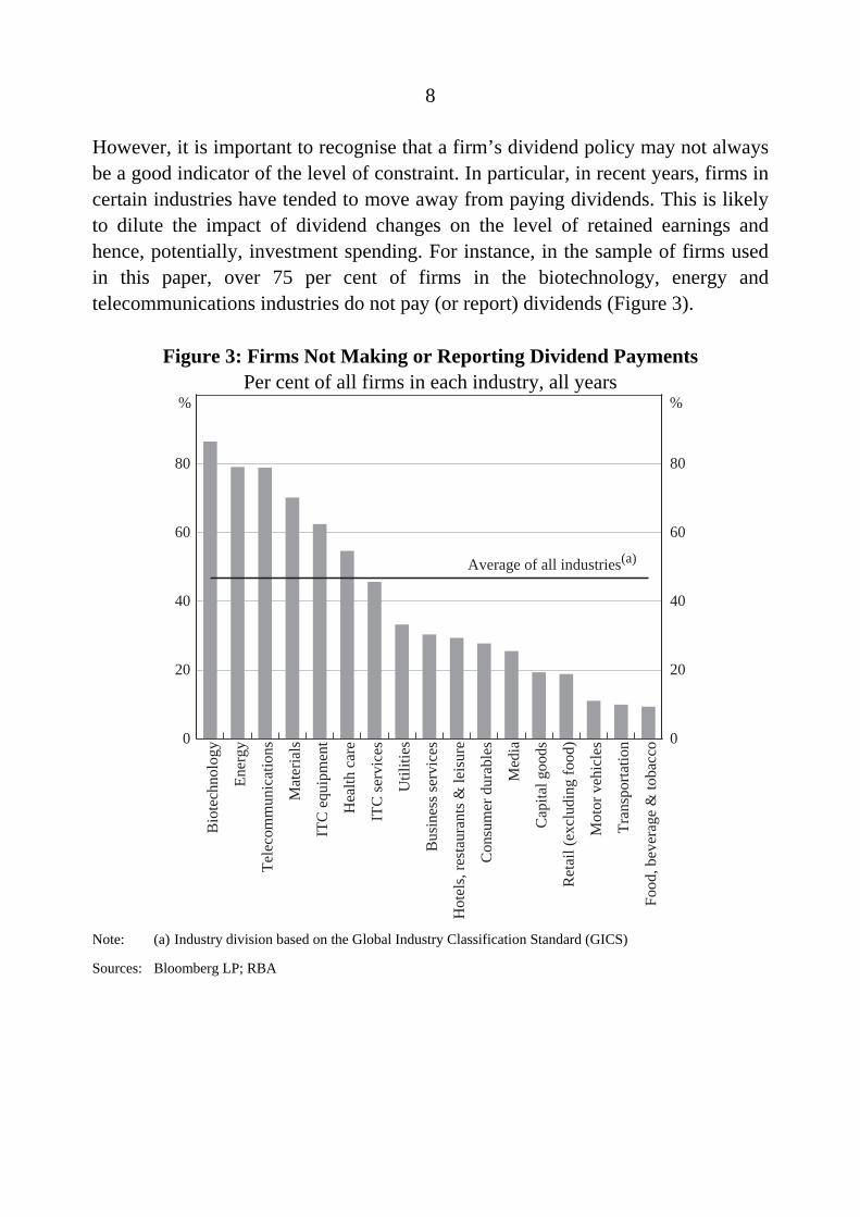
However, it is important to recognise that a firm’s dividend policy may not always be a good indicator of the level of constraint. In particular, in recent years, firms in certain industries have tended to move away from paying dividends. This is likely to dilute the impact of dividend changes on the level of retained earnings and hence, potentially, investment spending. For instance, in the sample of firms used in this paper, over 75 per cent of firms in the biotechnology, energy and telecommunications industries do not pay (or report) dividends (Figure 3).

Figure 3: Firms Not Making or Reporting Dividend Payments Per cent of all firms in each industry, all years

Bio

tech

nolo

gy

Ener

gy

Tele

com

mun

icat

ions

Mat

eria

ls

ITC

equ

ipm

ent

Hea

lth c

are

ITC

serv

ices

Util

ities

Bus

ines

s ser

vice

s

Hot

els,

rest

aura

nts &

leis

ure

Con

sum

er d

urab

les

Med

ia

Cap

ital g

oods

Ret

ail (

excl

udin

g fo

od)

Mot

or v

ehic

les

Tran

spor

tatio

n

Food

, bev

erag

e &

toba

cco0

20

40

60

80

0

20

40

60

80

Average of all industries(a)

%%

Note: (a) Industry division based on the Global Industry Classification Standard (GICS)

Sources: Bloomberg LP; RBA

9

Econometric analysis nonetheless suggests that dividend cutting is a useful measure of financial constraints in our data sample.6 One indication of this is that the proportion of firms identified as being financially constrained appears to be counter-cyclical, which seems fairly intuitive. I also experimented with other measures of financial constraints, including dividend payout ratios, firm size and age, the presence of corporate bond ratings and the firm’s implicit risk premium, measured as the difference between a firm’s average interest rate on debt and the risk-free interest rate (proxied by the yield on 10-year government bonds). The results of these exercises were qualitatively similar to those presented in this paper.

2.3 Financially Constrained versus Financially Distressed Firms

Assuming financial constraints are measured correctly, the preceding discussion implies that the investment of constrained firms should be more responsive to a given change in cash flow than the investment of unconstrained firms. However, a number of studies have found that the difference between the two groups is insignificant or that the investment of unconstrained firms is actually more responsive (Gilchrist and Himmelberg 1995; Kaplan and Zingales 1997; Cleary 1999; Allayannis and Mozumdar 2004).

One reason that constrained firms may not display a higher sensitivity to cash flow is because the sample of constrained firms could include firms that are in financial distress (Fazzari, Hubbard and Petersen 2000). Financially distressed firms can be thought of as those with negative cash flow. Such firms may be in such difficulty that they can only make absolutely essential investments so that any changes in investment in response to cash flow could be very limited. Even if their cash flow were to rise significantly, financially distressed firms have incentives to use the

6 In particular, I estimated a simple fixed-effects panel regression, regressing profitability (the

log of cash flow/assets) on year-fixed effects, industry dummies and a variable indicating dividend cuts (DIVCUT) under the hypothesis that the coefficient on DIVCUT should be negative and significant. The year-fixed effects should partly control for business cycle effects while the industry dummies should account for structural differences in dividend policies across sectors. The fact that I find a negative coefficient on the dividend cutting variable, which is significant at the 1 per cent level, implies that our measure of financial constraints is a reasonable proxy.

10

additional cash to reduce their debt levels, rather than using it for investment. As a result, the sensitivity of corporate investment to cash flow could be very low for these firms.7 If there are enough distressed firms in the sample, they may dampen the effect of cash flow on investment in an estimated model.

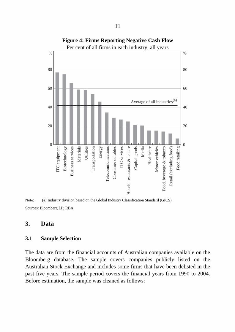
Empirically, such concerns also appear reasonable when considering the firms in the industries that account for most of the negative cash flow observations – generally firms in the ITC and biotechnology industries (Figure 4).8 These industries are characterised by firms that are generally young and growing rapidly, but which also face large start-up costs. For these firms, cash flow can be low (and falling) and the risk of default high even when prospects for future sales are good and the firms are investing heavily. Overall, these firms comprise over two-fifths of the sample and so will need to be accounted for in the estimated model.9

7 Another possible concern is the assumption of a positive (linear) relationship between

changes in cash flow and changes in investment. Some recent studies have argued that while changes in investment may be positively correlated with cash flow for certain levels of internal funding, at other levels, changes in investment may be negatively correlated with cash flow. In other words, a firm’s optimal investment function could be hump-shaped over a range of internal funding levels (Povel and Raith 2001; Allayannis and Mozumdar 2004; Cleary, Povel and Raith 2004; Cunningham 2004; Moyen 2004). However, I do not find compelling evidence for the hump-shaped hypothesis, which requires the investment of constrained firms to be sensitive to cash flow but also the investment of unconstrained and distressed firms to be relatively insensitive.

8 The measure of cash flow used in this paper is net profits after tax plus depreciation. If firms have engaged in new investment during the year, this will effectively reduce measured cash flow in that year. This is the standard measure used in the literature (for example, Von Kalckreuth 2001).

9 The overall proportion of firms reporting negative cash flow is much lower (though still quite high) in the final sample used in the regressions. This is because the exclusion criteria remove many of these firms from the final estimation (see Section 3.1).

11

Figure 4: Firms Reporting Negative Cash Flow Per cent of all firms in each industry, all years

ITC

equ

ipm

ent

Bio

tech

nolo

gy

Bus

ines

s ser

vice

s

Mat

eria

ls

Util

ities

Tran

spor

tatio

n

Ener

gy

Tele

com

mun

icat

ions

Con

sum

er d

urab

les

ITC

serv

ices

Hot

els,

rest

aura

nts &

leis

ure

Cap

ital g

oods

Med

ia

Hea

lthca

re

Mot

or v

ehic

les

Food

, bev

erag

e &

toba

cco

Ret

ail (

excl

udin

g fo

od)

Food

reta

iling

0

20

40

60

80

0

20

40

60

80

%%

Average of all industries(a)

Note: (a) Industry division based on the Global Industry Classification Standard (GICS)

Sources: Bloomberg LP; RBA

3. Data

3.1 Sample Selection

The data are from the financial accounts of Australian companies available on the Bloomberg database. The sample covers companies publicly listed on the Australian Stock Exchange and includes some firms that have been delisted in the past five years. The sample period covers the financial years from 1990 to 2004. Before estimation, the sample was cleaned as follows:

12

• banks, financial services, insurance and property trusts were removed (as the monetary policy transmission mechanism is likely to operate in a different manner for firms in the financial sector);

• firms with at least three consecutive years of financial accounts data within the sample period were retained; and

• for each variable in the model, the top and bottom 2 per cent of the distribution were trimmed to minimise the impact of outliers. However, for two variables, the investment rate and cash flow (as a share of capital), both the top and bottom 3 per cent of the distribution were trimmed.10

As will be seen, the estimation method also requires differencing the data, so that the first year of observations are lost. Controlling for possible endogeneity by using variables lagged over two years as instruments results in a final (unbalanced) panel of around 300 firms and 1 700 firm-year observations.

The non-random selection of the sample is likely to introduce several problems. For instance, the use of mainly listed companies means that the sample will be skewed towards larger firms. Assuming that larger firms are less likely to be constrained on average, this is likely to lower the estimated sensitivity of investment to cash flow. However, as will be seen in Section 4, it is not clear that this is necessarily the case.11

10 The additional trimming of these variables was needed to control for strong merger and

takeover activity and the information technology boom that occurred during the 1990s which affected the reported capital stock and profit figures of numerous companies. The extent of trimming is comparable to that seen in other overseas studies (for example, Von Kalckreuth 2001).

11 It is not immediately clear that the assumption of an inverse relationship between firm size and the level of financial constraints is a valid one. Recall that a financially constrained firm is one whose retained earnings are insufficient to match its investment opportunities. As a firm grows larger, it is not clear that a firm’s retained earnings will necessarily grow faster than its investment opportunities. However, economies of scale in credit management arguably imply that larger firms are less likely to be constrained on average. Also, smaller firms are more likely to be start-ups with little credit history, more subject to idiosyncratic risk and less likely to have developed a reputation with investors (Schiantarelli 1996).

13

Sources of company accounts data are also often subject to ‘survivor bias’. This occurs when delisted firms are removed from the sample, potentially giving a misleading picture of the corporate sector. However, this paper has the advantage over earlier Australian studies in that it includes some delisted companies. This minimises survivor bias and may better capture the effects of cash flow on firms that are probably financially distressed.12

Another potential problem in measuring investment with company accounts data is that firms that enter the sample satisfy certain selection criteria that may depend on unobservable factors that are likely to be correlated with investment and the business cycle. However, as will be discussed in Section 4, the econometric approach adopted should be able to control for these effects.

3.2 Variables in the Model

Appendix A summarises the construction of most of the variables used in the model. However, some variables are worth highlighting given their relative importance. The dependent variable is the investment rate, measured as the percentage change in the capital stock (after adding back depreciation). The explanatory variables include real sales (measured as firm-level sales revenue divided by the aggregate GDP deflator), cash flow and the real user cost of capital.

The calculation of the user cost of capital variable is relatively complex and is adapted from the measure constructed by Hall and Jorgenson (1967). The formula can be derived from neoclassical investment theory – a profit-maximising firm will accumulate capital up to the point where the marginal revenue from an extra unit of capital is just equal to the cost of employing that unit for the user. The user cost of capital incorporates not only the firm-specific cost of financing the purchase of capital (for example, through borrowing or new equity issues) but also sector-specific running costs (for example, depreciation rates) and other economy-wide variables (for example, corporate tax rates).

It is helpful to build the user cost of capital in a number of steps. First, assume that a representative firm finances the purchase or hire of capital through external

12 However, the improved coverage in the latter part of the sample introduces significant

heteroskedasticity in the data. This is controlled for in the estimation procedure.

14

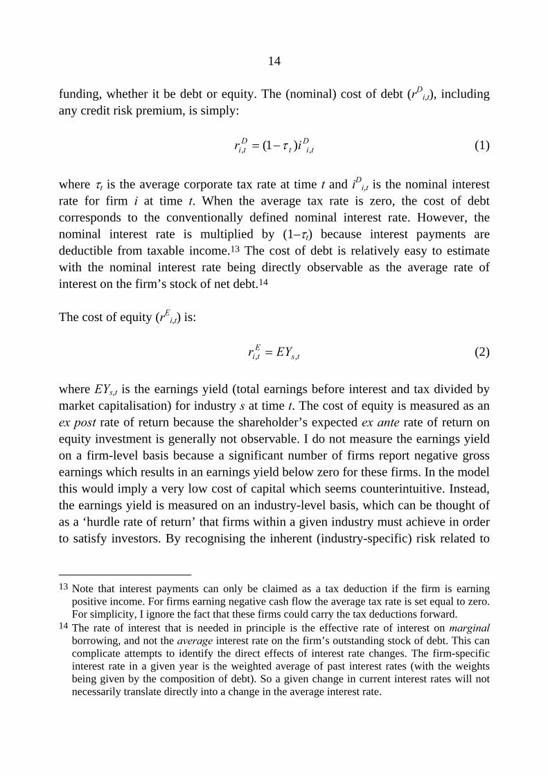
funding, whether it be debt or equity. The (nominal) cost of debt (rDi,t), including

any credit risk premium, is simply:

(1) Dtit

Dti ir ,, )1( τ−=

where τt is the average corporate tax rate at time t and iDi,t is the nominal interest

rate for firm i at time t. When the average tax rate is zero, the cost of debt corresponds to the conventionally defined nominal interest rate. However, the nominal interest rate is multiplied by (1–τt) because interest payments are deductible from taxable income.13 The cost of debt is relatively easy to estimate with the nominal interest rate being directly observable as the average rate of interest on the firm’s stock of net debt.14

The cost of equity (rEi,t) is:

(2) tsEti EYr ,, =

where EYs,t is the earnings yield (total earnings before interest and tax divided by market capitalisation) for industry s at time t. The cost of equity is measured as an ex post rate of return because the shareholder’s expected ex ante rate of return on equity investment is generally not observable. I do not measure the earnings yield on a firm-level basis because a significant number of firms report negative gross earnings which results in an earnings yield below zero for these firms. In the model this would imply a very low cost of capital which seems counterintuitive. Instead, the earnings yield is measured on an industry-level basis, which can be thought of as a ‘hurdle rate of return’ that firms within a given industry must achieve in order to satisfy investors. By recognising the inherent (industry-specific) risk related to

13 Note that interest payments can only be claimed as a tax deduction if the firm is earning

positive income. For firms earning negative cash flow the average tax rate is set equal to zero. For simplicity, I ignore the fact that these firms could carry the tax deductions forward.

14 The rate of interest that is needed in principle is the effective rate of interest on marginal borrowing, and not the average interest rate on the firm’s outstanding stock of debt. This can complicate attempts to identify the direct effects of interest rate changes. The firm-specific interest rate in a given year is the weighted average of past interest rates (with the weights being given by the composition of debt). So a given change in current interest rates will not necessarily translate directly into a change in the average interest rate.

15

equity investment, this measure should better reflect the cost of equity than simply using a long-term government bond rate, as in other studies (Gaiotti and Generale 2001; Chatelain and Tiomo 2001; Chatelain et al 2003). It also provides more cross-sectional variation in the data.15

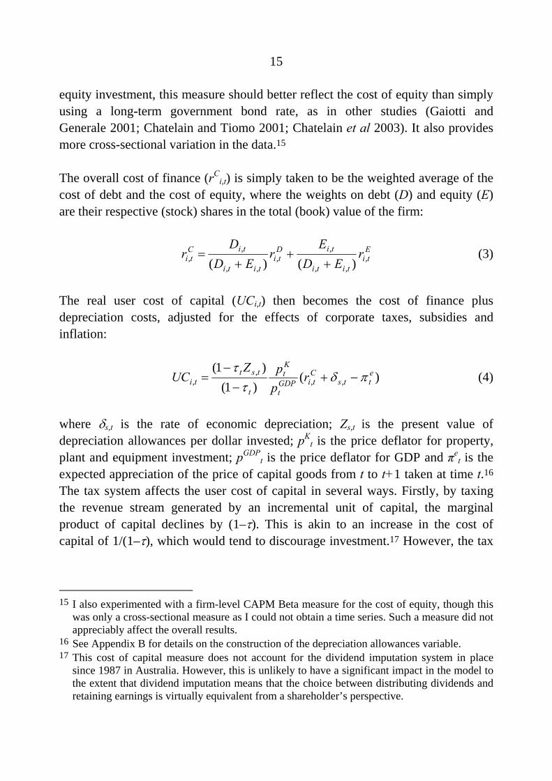
The overall cost of finance (rCi,t) is simply taken to be the weighted average of the

cost of debt and the cost of equity, where the weights on debt (D) and equity (E) are their respective (stock) shares in the total (book) value of the firm:

Eti

titi

tiDti

titi

tiCti r

EDE

rED

Dr ,

,,

,,

,,

,, )()( +

++

= (3)

The real user cost of capital (UCi,t) then becomes the cost of finance plus depreciation costs, adjusted for the effects of corporate taxes, subsidies and inflation:

)()1(

)1(,,

,,

etts

CtiGDP

t

Kt

t

tstti r

ppZ

UC πδτ

τ−+

−−

= (4)

where δs,t is the rate of economic depreciation; Zs,t is the present value of depreciation allowances per dollar invested; pK

t is the price deflator for property, plant and equipment investment; pGDP

t is the price deflator for GDP and πet is the

expected appreciation of the price of capital goods from t to t+1 taken at time t.16 The tax system affects the user cost of capital in several ways. Firstly, by taxing the revenue stream generated by an incremental unit of capital, the marginal product of capital declines by (1–τ). This is akin to an increase in the cost of capital of 1/(1–τ), which would tend to discourage investment.17 However, the tax

15 I also experimented with a firm-level CAPM Beta measure for the cost of equity, though this

was only a cross-sectional measure as I could not obtain a time series. Such a measure did not appreciably affect the overall results.

16 See Appendix B for details on the construction of the depreciation allowances variable. 17 This cost of capital measure does not account for the dividend imputation system in place

since 1987 in Australia. However, this is unlikely to have a significant impact in the model to the extent that dividend imputation means that the choice between distributing dividends and retaining earnings is virtually equivalent from a shareholder’s perspective.

16

system also allows various deductions that reduce the cost of capital and hence encourage investment. As we have already noted, corporate interest payments can be deducted for tax purposes, lowering the cost of debt. Also, the purchase price of a unit of capital is reduced by tax-depreciation allowances that can be claimed over time. Denoting the present value of deductions by Zs,t, the reduction in taxes is then given by (1–τZs,t).18

The user cost of capital is also affected by movements in capital goods prices. First, a higher price for capital goods relative to output prices increases the cost of installing the new capital, as captured by the term, pK

t/pGDPt. Second, if capital

goods prices are expected to increase over the coming period, then it pays to purchase the capital in the current period when it is cheaper. The firm can then benefit from the expected capital gain and, all other things being equal, this would reduce the user cost of capital for the firm. Expected capital goods price inflation is captured by the term, πe

t, which, in practice, is approximated by actual capital goods price inflation (Von Kalckreuth 2001).

3.3 Sample Characteristics and Comparisons to Aggregate Data

Before moving on to the econometric modelling, it is useful to examine the characteristics of the underlying sample of firms and to compare the firm-level data with data available at a more aggregated level. In terms of the number of firms, the final sample is about five times larger and covers a wider range of industries than previous Australian studies.19 The firm-level measures of investment, sales, user cost of capital and cash flow can also be compared with similar concepts at the aggregate level in order to assess the relative importance of this sample for aggregate investment and overall economic activity.

The (nominal) fixed investment, gross earnings and sales of firms in the sample constitute up to 70 per cent of their respective aggregate concepts, as reported in

18 The cost of capital is also effectively reduced by investment tax credits. However, these are

generally unavailable for investment in plant and equipment in Australia and so the tax credit is set equal to zero in the equation.

19 Details of the industry composition of the sample can be found in Appendix A.

17

the national accounts.20 Hence, these firms appear to explain a significant share of overall economic activity. It is also helpful to examine how investment, real sales, cash flow and the user cost of capital have moved at the aggregate level over the sample period and to compare these relationships with the measures at the firm level. The firm-level data are based on the median value for each year in order to minimise the impact of outliers.

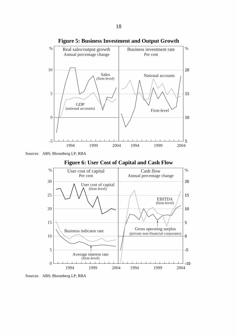
Not surprisingly given the smaller coverage, there tends to be more variability in the sample data than in the aggregate data. Still, movements in the firm-level measures of real sales growth and the rate of investment roughly appear to approximate the movements in the equivalent concepts at the aggregate level (Figure 5). Both measures appear to track the business cycle, with the firm-level measures clearly capturing the recession at the beginning of the sample period.

We can also see that the median user cost of capital has generally fallen over the 1990s, reflecting the gradual downward trend in borrowing rates, as illustrated by the business indicator rate in Figure 6.

There is a clear difference in the levels of, and movements in, the user cost of capital and the business indicator rate, reflecting the fact that the user cost of capital incorporates other costs such as depreciation and changes in capital goods prices. Stripping out these other factors and focusing just on the average interest rate embedded in the user cost measure, we can see a clearer correspondence with the indicator rate. Finally, there is also a fairly broad co-movement between the aggregate and firm-level measures of cash flow (Figure 6).

In summary, the aggregate and firm-level data appear reasonably well correlated over the sample period. As such, any significant relationships between investment, sales, cash flow and the user cost of capital uncovered at the microeconomic level are likely to provide insights into corresponding relationships at the macroeconomic level.

20 The aggregate concepts referred to are, specifically, gross investment in property, plant and

equipment, gross operating surplus for private non-financial corporations and GDP. The measure of GDP excludes government consumption and imputed dwelling rent in order to better approximate a measure of activity relevant to private non-financial corporations. The relative sizes of the sample aggregates vary on an annual basis, being generally lower in the earlier years because of poorer sample coverage.

18

Figure 5: Business Investment and Output Growth

-5

0

5

10

GDP

20045

10

15

20

5

10

15

20

(national accounts)

Real sales/output growthAnnual percentage change

Business investment ratePer cent

%%

Sales

Firm-level

National accounts(firm-level)

19991994200419991994 Sources: ABS; Bloomberg LP; RBA

Figure 6: User Cost of Capital and Cash Flow

0

5

10

15

20

25

30

Average interest rate

2004-10

-5

0

5

10

15

20

-10

-5

0

5

10

15

20

(firm-level)

User cost of capitalPer cent

Cash flowAnnual percentage change

%%

User cost of capital

Gross operating surplus

EBITDA

(firm-level)

(firm-level)

(private non-financial corporates)

19991994200419991994

Business indicator rate

Sources: ABS; Bloomberg LP; RBA

19

4. Modelling Strategy and Results

4.1 Estimation Method

Investment is typically a dynamic process, either because firms must develop some expectation of the likely future profitability of a project and/or because the nature of adjustment costs implies that it is cheaper for a firm to adjust its capital stock gradually.21 Models of business investment can generally be divided into two groups depending on whether the dynamics are modelled explicitly or implicitly. Explicit (or structural) models, such as the Tobin’s Q and Euler equations, allow dynamic elements to appear explicitly in the firm’s optimisation problem. These models have the benefit of directly linking the estimated coefficients to the underlying technology and expectation parameters (Chirinko 1993).

However, this paper focuses primarily on an implicit (or reduced form) model for several reasons. First, the main focus is to uncover the determinants of business investment rather than modelling the underlying technology or expectations formation processes. Second, while not explicitly derived, the investment equation still allows for short-run adjustment and expectation lags. Third, specifications similar to that used here have generally performed better than structural models in other microeconomic studies (Bond et al 1997; Chirinko, Fazzari and Meyer 1999; Von Kalckreuth 2001). Nevertheless, for comparability, I also estimate a Q-type model.22 Such a model assumes that the rate of investment is a function of Q – the ratio of the market value of new investment goods to their replacement cost. Under certain restrictive assumptions Q can be empirically measured using equity market data (Bond and Van Reenen 2003).23

21 This is true, for example, in the case of quadratic adjustment costs. 22 Despite being commonplace in micro studies of investment, the results of Q models have

generally been disappointing, often giving unreasonably low estimates of the effect of Q on investment (Bond and Van Reenen 2003). Furthermore, it is difficult to separately identify the interest rate and credit channels in a Q-type investment function. In practice, observable (average) Q is calculated from firms’ share prices, which are governed by fluctuations in asset prices and could therefore reflect either the interest rate or credit channel.

23 See Appendix A for details on the construction of the Q measure.

20

In constructing the main investment equation I start from the assumption that, in the absence of adjustment costs, the long-run equilibrium capital stock can be written as a (log-linear) function of real sales and the user cost of capital:

titititi ucyak ,,,, σρ −+= (5)

where ki,t is the (natural) log of firm i’s desired capital stock at time t, ai,t is an intercept term that captures productivity shocks, yi,t is the log of real sales, uci,t is the log of the firm’s user cost of capital and σ is the elasticity of substitution. This is consistent with profit maximisation subject to a constant elasticity of substitution (CES) production function and a single capital good. It allows for the possibility of constant returns to scale (ρ = 1), a fixed capital-output ratio (σ = 0), as well as the log-linear formulation with σ = 1, consistent with a Cobb-Douglas production function (Bond et al 2004).

The Error Correction Model (ECM) specification can be derived from this static capital demand equation. The procedure adopted here closely follows that of the existing literature (for example, Bond et al 1997). First, the equation is nested within a general dynamic regression model to account for the possibility of gradual adjustment of the capital stock to its long-run equilibrium.24 Productivity shocks are controlled for by including time-specific and firm-specific effects:

tii

T

jjj

tititititititititi

vd

ucucucyyykkk

,

1

1

2,21,1,02,21,1,02,21,1,

+++

+++++++=

∑−

=

−−−−−−

ηλ

γγγβββαα

(6)

where the dt’s are dummies to capture time-specific effects, ηi is a firm-specific effect, vi,t is a white noise error term and the time series runs from t = 1 to t = T. An assumption of constant returns to scale would require the restriction (β0+β1+β2)/ (1–α1–α2) = 1. Given the possible non-stationary nature of the data the equation is re-parameterised in error-correction form:

24 This implicitly assumes that the firm’s desired capital stock in the presence of adjustment

costs is proportional to its desired capital stock in the absence of adjustment costs, and that the short-run investment dynamics are stable enough over the sample period to be well approximated by the distributed lags in the regression model (Bond et al 1997).

21

tii

T

jjjtititi

tititi

tititi

vducucuc

yyy

kkk

,

1

12,2101,10,0

2,2101,10,0

2,121,1,

)()(

)()(

)1()1(

++++++∆++∆+

+++∆++∆+

−++∆−=∆

∑−

=−−

−−

−−

ηλγγγγγγ

ββββββ

ααα

(7)

Letting Ii,t denote gross investment, Ki,t the capital stock, and δi,t the depreciation rate, we can then use the approximation !ki,t = (Ii,t/Ki,t–1–δi,t) to obtain an ECM specification for the investment rate (Ii,t/Ki,t–1).25 To investigate the role of financial constraints, we also include current and lagged cash flow (CFi,t) terms in the equation.26 The ECM becomes:

iti

T

jjj

ti

ti

ti

ti

tititi

ti

titititi

ti

ti

ti

vdKCF

KCF

ucucuc

y

yykKI

KI

+++++

+++∆++∆+

+++

∆++∆+−++−=

∑−

=−

−

−

−−

−

−−−

−

−

ηλθθ

γγγγγγ

βββ

βββααα

1

12,

1,2

1,

,1

2,2101,10,0

2,210

1,10,02,122,

1,1

1,

,

)()(

)()(

)(

)()1())(1(

(8)

In Equation (8), the coefficient on the speed of adjustment term (α2+α1–1) is expected to be negative, as the firm should reduce investment if it has excess capacity. Financial constraints are modelled by augmenting the basic ECM of Equation (8) in one of two ways. The first is to use a dummy variable (DIVCUT) to identify financially constrained firms. This is equal to one if the firm has cut dividends (in either the current or previous year) and zero otherwise. This dummy is interacted with the cash flow variable to capture any differential effect of cash

25 The term, !ki,t, is the change in the log(Ki,t) which is roughly equal to the percent change in

Ki,t. This, in turn, is approximately equal to (Ii,t/Ki,t–1–δi,t). The depreciation rate, δi,t, can be subsumed into some combination of the last three terms in Equation (8), allowing !ki,t to be replaced with Ii,t/Ki,t�1.

26 Heteroskedasticity can be a problem with company accounts data. The cash flow and investment variables are scaled by the previous period’s net capital stock to minimise its effect (for example, through firm size effects). Estimating with robust standard errors should control for any additional effects of heteroskedasticity.

22

flow for financially constrained firms. These variables are denoted as DIVCUT*CF/K. The coefficients on the cash flow terms by themselves will capture the responsiveness of investment to cash flow for unconstrained firms (theory implies that these coefficients will be zero). The responsiveness of investment to cash flow for constrained firms is then given by the combination of the coefficients (θ1 and θ2) and the coefficients on the interactive DIVCUT*CF/K variables. The coefficients on these interactive terms are expected to be jointly significant and positively signed if financially constrained firms respond more strongly to cash flow than unconstrained firms.

As discussed in Section 2.2, the presence of distressed firms within the constrained group may bias the coefficient on these interactive terms. This bias could be significant given that negative cash flow (acting as a proxy for financial distress) occurs in around 15 per cent of the firm-year observations used in the model. The second way of augmenting the basic ECM attempts to deal with this problem by separating the financially constrained group into those earning positive and negative cash flow. This is done by the use of three separate dummies, again all interacting with the cash flow variable. The first dummy takes the value of one if the firm has cut dividends but earns positive cash flow (financially constrained, FC) and zero otherwise.27 The second dummy takes the value of one if the firm has cut dividends and has made a loss during the year (financially distressed, FD) and zero otherwise. I include a third dummy for firms that have made losses but not cut dividends, a group I refer to as ‘loss-makers’ (LM). These firms are technically financially distressed but have not cut dividends, perhaps because they operate in industries that do not pay dividends (as we saw in Section 2.2) or because dividend cuts act as a signal of weak profitability to investors. The remaining group of firms that have positive cash flow are then classified as unconstrained (UC).

These two approaches are summarised in Table 1. The first approach divides the sample into two parts, those that have cut dividends (the first column) and those that have not (the second column). The second approach makes a further distinction by splitting firms on the basis of positive versus negative cash flow (the top and bottom rows respectively).

27 Here, and in what follows, this refers to dividend cuts and cash flow of the current and the

previous year.

23

Table 1: Classification of Firm-year Observations Numbers (percentages) of each group

Indicator of financial constraint Dividend cut No dividend cut

Positive cash flow

346 (19.8%) FC � constrained

1 141 (65.4%) UC � unconstrained

Indicator of financial distress

Negative cash flow

98 (5.6%) FD � distressed

160 (9.2%) LM � loss-makers

1 745 (100%)

For comparability, I also estimate a structural Q-type Equation (Q1):

tii

T

jjj

ti

titi

ti

ti vdKCF

QKI

,

1

11,

,1,

1,

, )( ++++= ∑−

=−−

−

ηλθβ (9)

where all variables are as denoted before, with the addition of Qi,t�1 which represents the firm’s average Q, measured as the market value of the firm’s equity divided by the book value of the firm’s equity. Constrained firms are accounted for by using the two sets of dummy variables described above. The results from estimating both the ECM and the Q model are outlined in Section 4.3. Before turning to the results, some econometric issues specific to panel-data models need to be briefly addressed.

4.2 Other Modelling Issues

Panel-data models are usually estimated using either ‘fixed effects’ or ‘random effects’ techniques. In this paper, a form of fixed-effects estimation is adopted because firm-specific effects are likely to be present, either as a result of technological heterogeneity or non-random sampling, with these likely to be correlated with the explanatory variables (for example, managerial skills could be correlated with the level of cash flow). This approach can yield consistent

24

estimates even if the firm-specific error components and the explanatory variables are correlated.28 This is the approach taken to estimate the Q model.

However, the issue is complicated in dynamic panels with a finite time horizon, such as the ECM. In this case, fixed-effects estimation is inconsistent because the lagged dependent variable is correlated with the error term. As a result, the ECM is estimated using the Arellano-Bond two-step Generalised Method of Moments (GMM) estimator which is consistent in this dynamic setting. This estimation technique eliminates firm-specific effects by differencing the equations, and then uses lagged values of endogenous variables as instruments. If the error term in levels is serially uncorrelated, then the error term in first differences is MA(1), and instruments dated (t–2) periods and earlier should be valid. Under this assumption, consistent parameter estimates can be obtained. The validity of the instruments is tested by reporting both a Sargan test of the over-identifying restrictions, and direct tests of serial correlation in the residuals.

4.3 Results

The complete list of coefficient estimates, standard errors, and levels of significance for four separate versions of the ECM are presented in Tables 2 and 3. The first model (EC1) is the standard ECM without cash flow in the formulation. The second model (EC2) then includes cash flow. The third and fourth models (EC3 and EC4) are as per EC2 but augmented with the two different sets of dummy variables interacted with the cash flow variable as described above.

As can be seen in Table 2, the coefficient on the lagged investment rate is negative and significant across all four models, suggesting that investment is negatively correlated across successive time periods. This implies that ‘bursts’ of investment do not spill over to consecutive years, but are followed by lower investment rates in the future, on average. The speed of adjustment parameter is also of the expected (negative) sign implying that firms with excess capacity cut back on their investment plans.

28 While a consistent estimator, the use of many dummy variables means the fixed-effects

estimator is less efficient than the random-effects estimator.

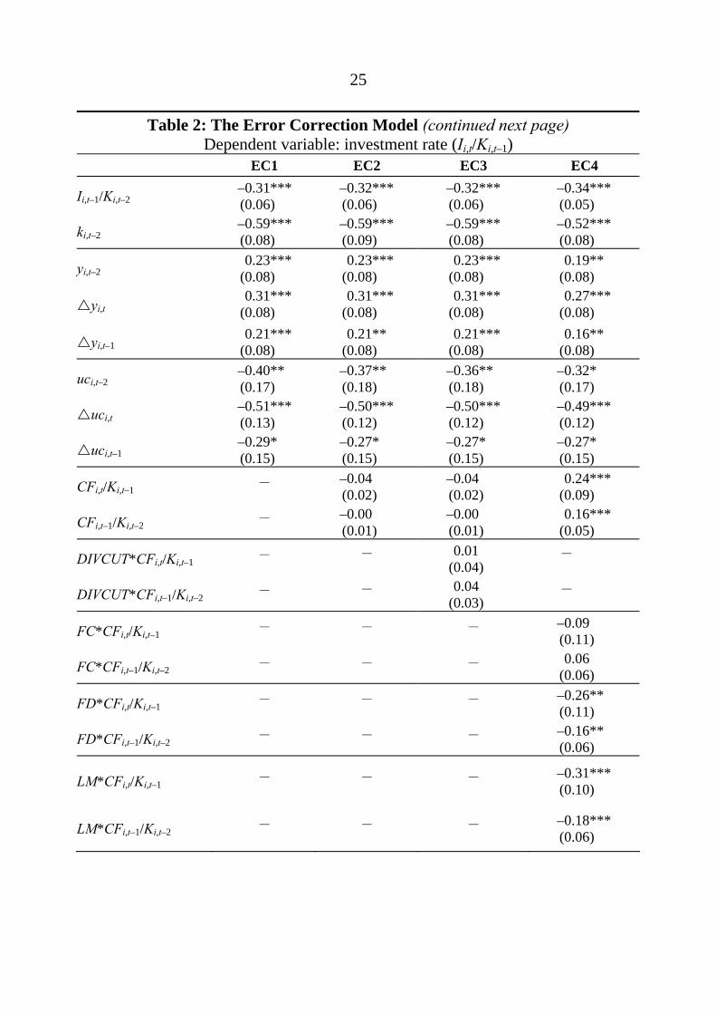
25

Table 2: The Error Correction Model (continued next page) Dependent variable: investment rate (Ii,t/Ki,t–1)

EC1 EC2 EC3 EC4

Ii,t–1/Ki,t–2 –0.31*** (0.06)

–0.32*** (0.06)

–0.32*** (0.06)

–0.34*** (0.05)

ki,t–2 –0.59*** (0.08)

–0.59*** (0.09)

–0.59*** (0.08)

–0.52*** (0.08)

yi,t–2 0.23***

(0.08) 0.23***

(0.08) 0.23***

(0.08) 0.19**

(0.08)

!yi,t 0.31***

(0.08) 0.31***

(0.08) 0.31***

(0.08) 0.27***

(0.08)

!yi,t–1 0.21***

(0.08) 0.21**

(0.08) 0.21***

(0.08) 0.16**

(0.08)

uci,t–2 –0.40** (0.17)

–0.37** (0.18)

–0.36** (0.18)

–0.32* (0.17)

!uci,t –0.51*** (0.13)

–0.50*** (0.12)

–0.50*** (0.12)

–0.49*** (0.12)

!uci,t–1 –0.29* (0.15)

–0.27* (0.15)

–0.27* (0.15)

–0.27* (0.15)

CFi,t/Ki,t–1 — –0.04 (0.02)

–0.04 (0.02)

0.24*** (0.09)

CFi,t–1/Ki,t–2 — –0.00 (0.01)

–0.00 (0.01)

0.16*** (0.05)

DIVCUT*CFi,t/Ki,t–1 — — 0.01 (0.04)

—

DIVCUT*CFi,t–1/Ki,t–2 — — 0.04 (0.03)

—

FC*CFi,t/Ki,t–1 — — — –0.09 (0.11)

FC*CFi,t–1/Ki,t–2 — — — 0.06 (0.06)

FD*CFi,t/Ki,t–1 — — — –0.26** (0.11)

FD*CFi,t–1/Ki,t–2 — — — –0.16** (0.06)

LM*CFi,t/Ki,t–1 — — — –0.31*** (0.10)

LM*CFi,t–1/Ki,t–2 — — — –0.18*** (0.06)

26

Table 2: The Error Correction Model (continued) Memoranda

Long-run elasticity of output growth 0.40*** 0.38*** 0.39*** 0.37***

Long-run elasticity of the user cost of capital –0.67** –0.62** –0.60** –0.62**

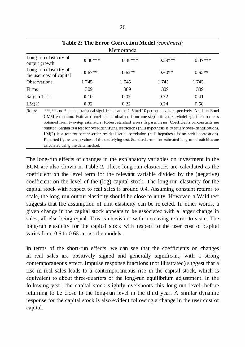
Observations 1 745 1 745 1 745 1 745 Firms 309 309 309 309 Sargan Test 0.10 0.09 0.22 0.41 LM(2) 0.32 0.22 0.24 0.58 Notes: ***, ** and * denote statistical significance at the 1, 5 and 10 per cent levels respectively. Arellano-Bond

GMM estimation. Estimated coefficients obtained from one-step estimators. Model specification tests obtained from two-step estimators. Robust standard errors in parentheses. Coefficients on constants areomitted. Sargan is a test for over-identifying restrictions (null hypothesis is to satisfy over-identification). LM(2) is a test for second-order residual serial correlation (null hypothesis is no serial correlation).Reported figures are p-values of the underlying test. Standard errors for estimated long-run elasticities are calculated using the delta method.

The long-run effects of changes in the explanatory variables on investment in the ECM are also shown in Table 2. These long-run elasticities are calculated as the coefficient on the level term for the relevant variable divided by the (negative) coefficient on the level of the (log) capital stock. The long-run elasticity for the capital stock with respect to real sales is around 0.4. Assuming constant returns to scale, the long-run output elasticity should be close to unity. However, a Wald test suggests that the assumption of unit elasticity can be rejected. In other words, a given change in the capital stock appears to be associated with a larger change in sales, all else being equal. This is consistent with increasing returns to scale. The long-run elasticity for the capital stock with respect to the user cost of capital varies from 0.6 to 0.65 across the models.

In terms of the short-run effects, we can see that the coefficients on changes in real sales are positively signed and generally significant, with a strong contemporaneous effect. Impulse response functions (not illustrated) suggest that a rise in real sales leads to a contemporaneous rise in the capital stock, which is equivalent to about three-quarters of the long-run equilibrium adjustment. In the following year, the capital stock slightly overshoots this long-run level, before returning to be close to the long-run level in the third year. A similar dynamic response for the capital stock is also evident following a change in the user cost of capital.

27

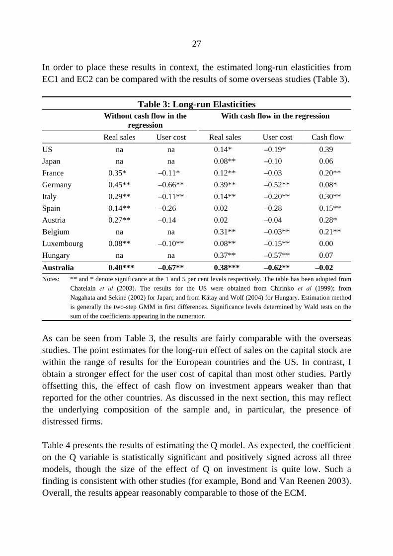
In order to place these results in context, the estimated long-run elasticities from EC1 and EC2 can be compared with the results of some overseas studies (Table 3).

Table 3: Long-run Elasticities Without cash flow in the

regression With cash flow in the regression

Real sales User cost Real sales User cost Cash flow US na na 0.14* –0.19* 0.39 Japan na na 0.08** –0.10 0.06 France 0.35* –0.11* 0.12** –0.03 0.20** Germany 0.45** –0.66** 0.39** –0.52** 0.08* Italy 0.29** –0.11** 0.14** –0.20** 0.30** Spain 0.14** –0.26 0.02 –0.28 0.15** Austria 0.27** –0.14 0.02 –0.04 0.28* Belgium na na 0.31** –0.03** 0.21** Luxembourg 0.08** –0.10** 0.08** –0.15** 0.00 Hungary na na 0.37** –0.57** 0.07 Australia 0.40*** –0.67** 0.38*** –0.62** –0.02 Notes: ** and * denote significance at the 1 and 5 per cent levels respectively. The table has been adopted from

Chatelain et al (2003). The results for the US were obtained from Chirinko et al (1999); from Nagahata and Sekine (2002) for Japan; and from Kátay and Wolf (2004) for Hungary. Estimation method is generally the two-step GMM in first differences. Significance levels determined by Wald tests on the sum of the coefficients appearing in the numerator.

As can be seen from Table 3, the results are fairly comparable with the overseas studies. The point estimates for the long-run effect of sales on the capital stock are within the range of results for the European countries and the US. In contrast, I obtain a stronger effect for the user cost of capital than most other studies. Partly offsetting this, the effect of cash flow on investment appears weaker than that reported for the other countries. As discussed in the next section, this may reflect the underlying composition of the sample and, in particular, the presence of distressed firms.

Table 4 presents the results of estimating the Q model. As expected, the coefficient on the Q variable is statistically significant and positively signed across all three models, though the size of the effect of Q on investment is quite low. Such a finding is consistent with other studies (for example, Bond and Van Reenen 2003). Overall, the results appear reasonably comparable to those of the ECM.

28

Table 4: The Q Model Q1 Q2 Q3

Qi,t–1 0.01***

(0.00) 0.01***

(0.00) 0.01***

(0.00)

CFi,t/Ki,t–1 –0.01** (0.00)

–0.01** (0.00)

0.35*** (0.03)

DIVCUT*CFi,t/Ki,t–1 — 0.04* (0.02)

—

FC*CFi,t/Ki,t–1 — — 0.08 (0.07)

FD*CFi,t/Ki,t–1 — — –0.39*** (0.04)

LM*CFi,t/Ki,t–1 — — –0.37*** (0.03)

Observations 2 595 2 595 2 595 Firms 391 391 391 Within R2 0.081 0.084 0.142 Notes: ***, ** and * denote statistical significance at the 1, 5 and 10 per cent levels respectively. Fixed-effects

estimation. Robust standard errors in parentheses. Coefficients on constants are omitted.

4.4 The Effect of Financial Constraints and Financial Distress

We are now in a position to assess the effect of financial constraints and distress on corporate investment in the models. In discussing the results, I generally focus on the preferred model, the ECM; most of the results from the Q model are broadly comparable.

Based on the results of the model EC2, cash flow appears to have a negligible influence on the investment rate, with the coefficients on cash flow negatively signed at both lags but not significantly different from zero (Table 2). Other parameter estimates appear robust to the inclusion of this variable. In contrast, the results of estimating the model Q2 suggest that the inverse relationship between cash flow and investment is statistically significant (Table 4). It is not clear why controlling for investment opportunities through the use of Q should necessarily lead to a significant negative correlation between cash flow and investment. It may simply reflect the fact that the size of the underlying sample differs between the two models, being somewhat larger in the Q model than in the ECM.

29

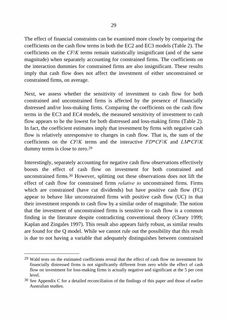
The effect of financial constraints can be examined more closely by comparing the coefficients on the cash flow terms in both the EC2 and EC3 models (Table 2). The coefficients on the CF/K terms remain statistically insignificant (and of the same magnitude) when separately accounting for constrained firms. The coefficients on the interaction dummies for constrained firms are also insignificant. These results imply that cash flow does not affect the investment of either unconstrained or constrained firms, on average.

Next, we assess whether the sensitivity of investment to cash flow for both constrained and unconstrained firms is affected by the presence of financially distressed and/or loss-making firms. Comparing the coefficients on the cash flow terms in the EC3 and EC4 models, the measured sensitivity of investment to cash flow appears to be the lowest for both distressed and loss-making firms (Table 2). In fact, the coefficient estimates imply that investment by firms with negative cash flow is relatively unresponsive to changes in cash flow. That is, the sum of the coefficients on the CF/K terms and the interactive FD*CF/K and LM*CF/K dummy terms is close to zero.29

Interestingly, separately accounting for negative cash flow observations effectively boosts the effect of cash flow on investment for both constrained and unconstrained firms.30 However, splitting out these observations does not lift the effect of cash flow for constrained firms relative to unconstrained firms. Firms which are constrained (have cut dividends) but have positive cash flow (FC) appear to behave like unconstrained firms with positive cash flow (UC) in that their investment responds to cash flow by a similar order of magnitude. The notion that the investment of unconstrained firms is sensitive to cash flow is a common finding in the literature despite contradicting conventional theory (Cleary 1999; Kaplan and Zingales 1997). This result also appears fairly robust, as similar results are found for the Q model. While we cannot rule out the possibility that this result is due to not having a variable that adequately distinguishes between constrained

29 Wald tests on the estimated coefficients reveal that the effect of cash flow on investment for

financially distressed firms is not significantly different from zero while the effect of cash flow on investment for loss-making firms is actually negative and significant at the 5 per cent level.

30 See Appendix C for a detailed reconciliation of the findings of this paper and those of earlier Australian studies.

30

and unconstrained firms, using other indicators of financial constraints (such as size, age and the presence of bond ratings) does not alter the main findings.

5. Conclusion

The effects of financial factors on corporate investment are estimated using a large sample of listed Australian companies over the period 1990 to 2004. Real sales and the user cost of capital appear to be significant determinants of firm-level investment in both the short and long run.

Theory suggests that internal funding should affect investment if some firms are financially constrained and cannot obtain enough external funding to meet their desired level of investment. However, this paper suggests that, across all firms, the response of investment to cash flow is minimal, whether or not the firms are financially constrained. However, there is evidence that this result may reflect the presence of firms experiencing financial distress (as indicated by the presence of negative cash flow). Among non-distressed firms, the investment response to cash flow is found to be positive, with the estimated sensitivity being roughly the same for both constrained and unconstrained firms. In summary, these results partly contradict the conventional view of the credit channel, and are in contrast to the results of Australian studies using data largely from the 1980s. Nevertheless, they are consistent with the findings of recent international studies.

31

Appendix A: Variable Definitions, Sources and Summary Statistics

Table A1: Summary of Variable Definitions Net capital stock (K) According to the perpetual inventory method (see Appendix B).Investment rate (I/K) (Net capital stock in current period – net capital stock in

previous period – fixed asset revaluations + depreciation)/net capital stock in previous period.

Depreciation rate (δ) Depreciation expenses/net capital stock. Calculated at industry level.

Depreciation allowances (Z) See Appendix B for details of calculations. Capital goods price deflator (PK) Implicit price deflator for property, plant and equipment,

ABS Cat No 5206.0. Output price deflator (PY) GDP deflator, ABS Cat No 5206.0. Corporate tax rate (τ) Corporate marginal tax rates, Australian Taxation Office. Average interest rate (i) Interest expenses/debt. User cost of capital (UC) According to Equations (1–4). Sales (S) Total sales or trading revenue. Output (Y) Total sales revenue/output price deflator. Cash flow (CF) Net profits after tax + depreciation expenses. Cash flow to capital ratio (CF/K) Cash flow/net capital stock in previous period. Dividend cutting dummy (DIVCUT)

Equals one if firm has cut dividends in the current and/or previous period; zero otherwise.

Financially constrained dummy (FC)

Equals one if firm has cut dividends in the current and/or previous period and reports cash flow > 0; zero otherwise.

Financially distressed dummy (FC)

Equals one if firm has cut dividends in the current and/or previous period and reports cash flow < 0; zero otherwise.

Loss maker dummy (LM) Equals one if firm has not cut dividends in the current and/or previous period but reports cash flow < 0; zero otherwise.

Book value of assets (A) Total assets. Market capitalisation / market value of equity (MKTCAP)

Product of the number of outstanding shares and the year-ended share price.

Book value of equity (E) Total assets – total liabilities. Debt (D) Short-term + long-term debt from financial institutions and

financial leases + non-current convertible notes. Book value is taken as a proxy for market value.

Liquid assets (CASH) Stock of cash and its equivalent, including cash on hand, cash and short-term deposits held at financial institutions.

Tobin’s Q (Q) (Market value of equity + book value of debt – cash) / (net capital stock at replacement cost + inventories). See Mills et al (1994) for further details.

32

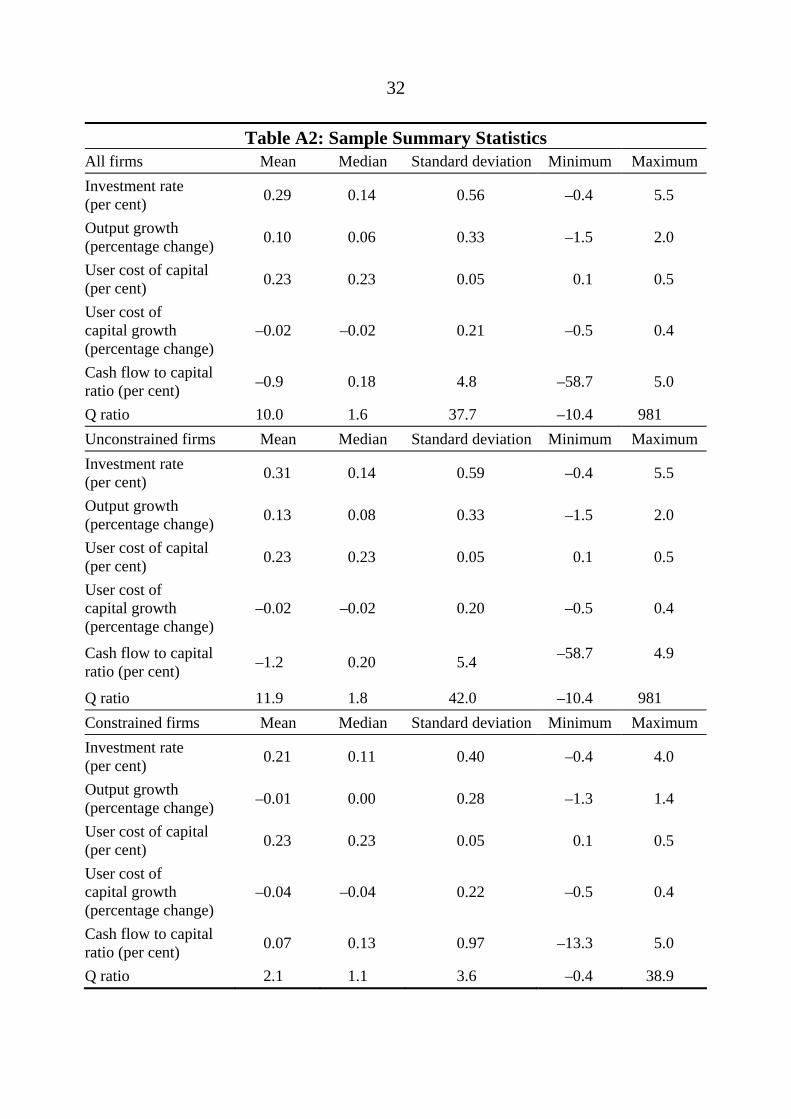
Table A2: Sample Summary Statistics All firms Mean Median Standard deviation Minimum Maximum Investment rate (per cent) 0.29 0.14 0.56 –0.4 5.5

Output growth (percentage change) 0.10 0.06 0.33 –1.5 2.0

User cost of capital (per cent) 0.23 0.23 0.05 0.1 0.5

User cost of capital growth (percentage change)

–0.02 –0.02 0.21 –0.5 0.4

Cash flow to capital ratio (per cent) –0.9 0.18 4.8 –58.7 5.0

Q ratio 10.0 1.6 37.7 –10.4 981 Unconstrained firms Mean Median Standard deviation Minimum Maximum Investment rate (per cent) 0.31 0.14 0.59 –0.4 5.5

Output growth (percentage change) 0.13 0.08 0.33 –1.5 2.0

User cost of capital (per cent) 0.23 0.23 0.05 0.1 0.5

User cost of capital growth (percentage change)

–0.02 –0.02 0.20 –0.5 0.4

Cash flow to capital ratio (per cent) –1.2 0.20 5.4 –58.7 4.9

Q ratio 11.9 1.8 42.0 –10.4 981 Constrained firms Mean Median Standard deviation Minimum Maximum Investment rate (per cent) 0.21 0.11 0.40 –0.4 4.0

Output growth (percentage change) –0.01 0.00 0.28 –1.3 1.4

User cost of capital (per cent) 0.23 0.23 0.05 0.1 0.5

User cost of capital growth (percentage change)

–0.04 –0.04 0.22 –0.5 0.4

Cash flow to capital ratio (per cent) 0.07 0.13 0.97 –13.3 5.0

Q ratio 2.1 1.1 3.6 –0.4 38.9

33

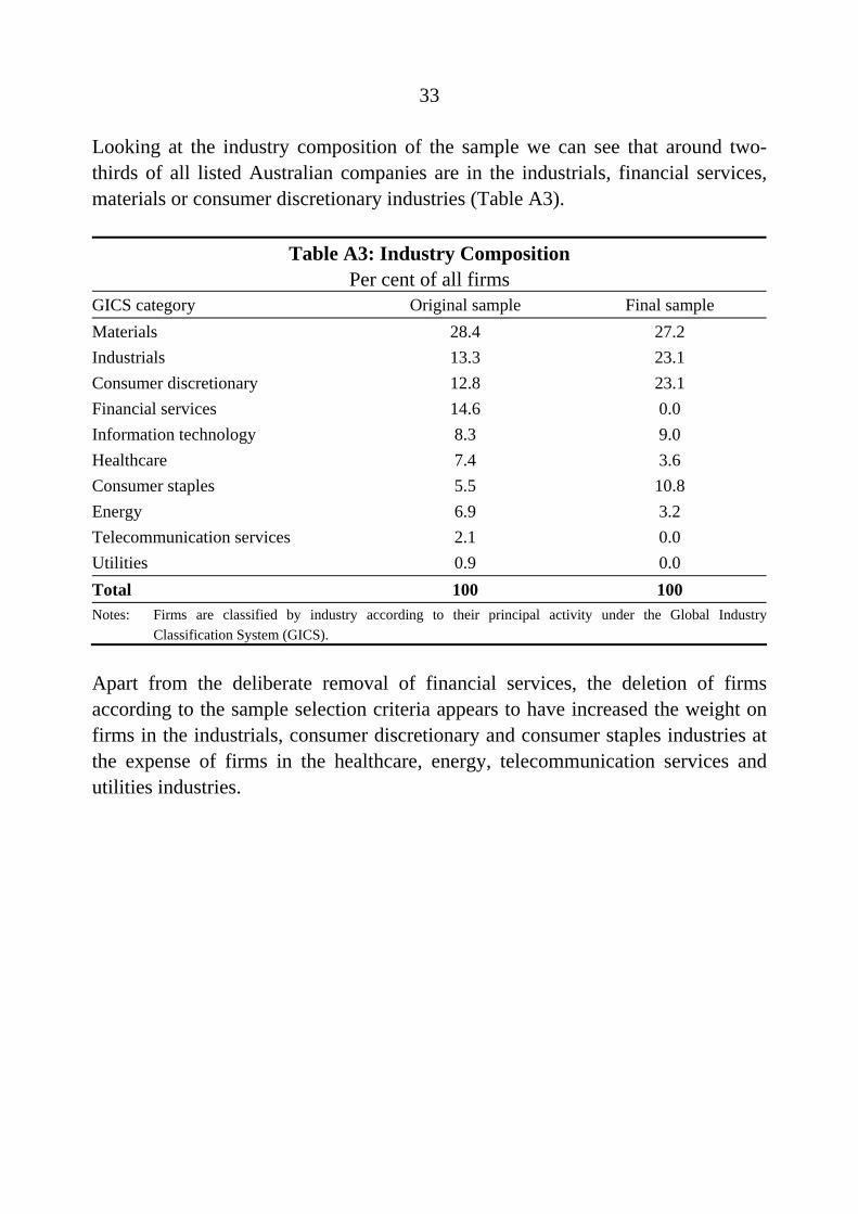
Looking at the industry composition of the sample we can see that around two-thirds of all listed Australian companies are in the industrials, financial services, materials or consumer discretionary industries (Table A3).

Table A3: Industry Composition Per cent of all firms

GICS category Original sample Final sample Materials 28.4 27.2 Industrials 13.3 23.1 Consumer discretionary 12.8 23.1 Financial services 14.6 0.0 Information technology 8.3 9.0 Healthcare 7.4 3.6 Consumer staples 5.5 10.8 Energy 6.9 3.2 Telecommunication services 2.1 0.0 Utilities 0.9 0.0 Total 100 100 Notes: Firms are classified by industry according to their principal activity under the Global Industry

Classification System (GICS).

Apart from the deliberate removal of financial services, the deletion of firms according to the sample selection criteria appears to have increased the weight on firms in the industrials, consumer discretionary and consumer staples industries at the expense of firms in the healthcare, energy, telecommunication services and utilities industries.

34

Appendix B: Measurement Issues

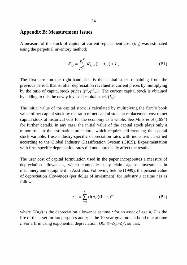
A measure of the stock of capital at current replacement cost (Ki,t) was estimated using the perpetual inventory method:

titstiKt

Kt

ti IKppK ,,1,

1, )1( +−= −

−

δ (B1)

The first term on the right-hand side is the capital stock remaining from the previous period, that is, after depreciation revalued at current prices by multiplying by the ratio of capital stock prices (pK

t/pKt–1). The current capital stock is obtained

by adding to this the newly invested capital stock (Ii,t).

The initial value of the capital stock is calculated by multiplying the firm’s book value of net capital stock by the ratio of net capital stock at replacement cost to net capital stock at historical cost for the economy as a whole. See Mills et al (1994) for further details. In any case, the initial value of the capital stock plays only a minor role in the estimation procedure, which requires differencing the capital stock variable. I use industry-specific depreciation rates with industries classified according to the Global Industry Classification System (GICS). Experimentation with firm-specific depreciation rates did not appreciably affect the results.

The user cost of capital formulation used in the paper incorporates a measure of depreciation allowances, which companies may claim against investment in machinery and equipment in Australia. Following Sekine (1999), the present value of depreciation allowances (per dollar of investment) for industry s at time t is as follows:

(B2) ∑=

−+=T

n

ntts rtnDz

1, )1)(,(

where D(n,t) is the depreciation allowance at time t for an asset of age n, T is the life of the asset for tax purposes and rt is the 10-year government bond rate at time t. For a firm using exponential depreciation, D(n,t)=δ(1–δ)n, so that:

35

δ

δ++

=t

tts r

rz

)1(, (B3)

For a firm using straight-line depreciation, D(n,t)=1/T for an existing asset and D(n,t) = 0 for a retired asset so that:

Tr

rrz

t

Ttt

ts])1(1)[1(

,

−+−+= (B4)

As we cannot identify a given firm’s method of depreciation, we simply take an average of the two methods to obtain the present value of depreciation allowances for each industry in each year.

36

Appendix C: Comparisons with Earlier Australian Studies

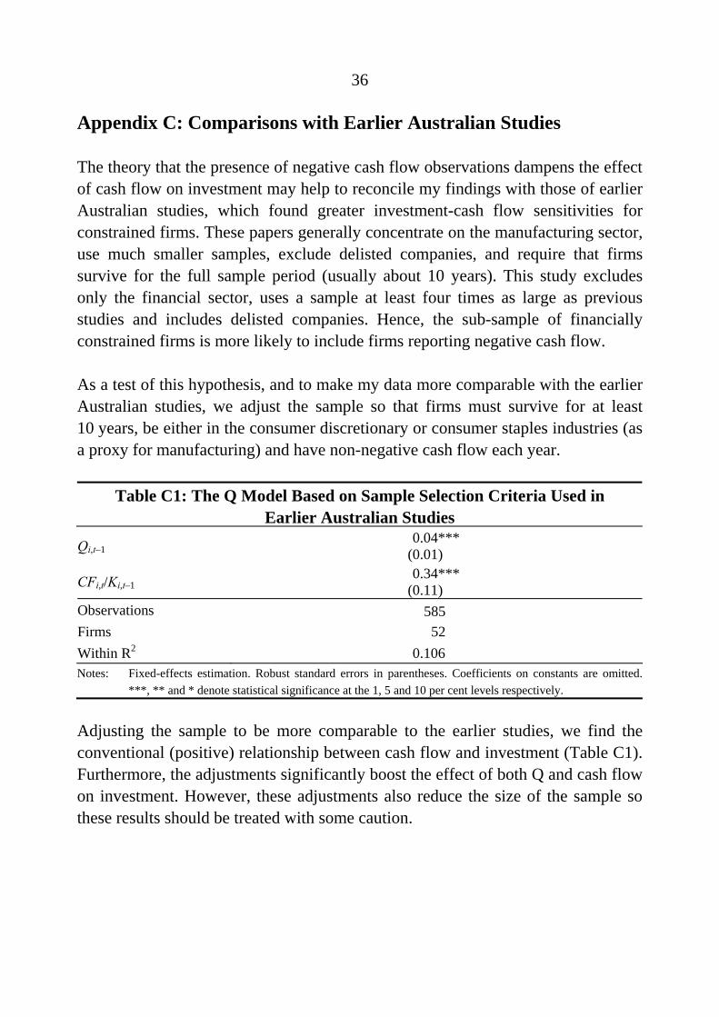
The theory that the presence of negative cash flow observations dampens the effect of cash flow on investment may help to reconcile my findings with those of earlier Australian studies, which found greater investment-cash flow sensitivities for constrained firms. These papers generally concentrate on the manufacturing sector, use much smaller samples, exclude delisted companies, and require that firms survive for the full sample period (usually about 10 years). This study excludes only the financial sector, uses a sample at least four times as large as previous studies and includes delisted companies. Hence, the sub-sample of financially constrained firms is more likely to include firms reporting negative cash flow.

As a test of this hypothesis, and to make my data more comparable with the earlier Australian studies, we adjust the sample so that firms must survive for at least 10 years, be either in the consumer discretionary or consumer staples industries (as a proxy for manufacturing) and have non-negative cash flow each year.

Table C1: The Q Model Based on Sample Selection Criteria Used in Earlier Australian Studies

Qi,t–1 0.04***

(0.01)

CFi,t/Ki,t–1 0.34***

(0.11) Observations 585 Firms 52 Within R2 0.106 Notes: Fixed-effects estimation. Robust standard errors in parentheses. Coefficients on constants are omitted.

***, ** and * denote statistical significance at the 1, 5 and 10 per cent levels respectively.

Adjusting the sample to be more comparable to the earlier studies, we find the conventional (positive) relationship between cash flow and investment (Table C1). Furthermore, the adjustments significantly boost the effect of both Q and cash flow on investment. However, these adjustments also reduce the size of the sample so these results should be treated with some caution.

37

References

Allayannis G and A Mozumdar (2004), ‘The impact of negative cash flow and influential observations on investment-cash flow sensitivity estimates’, Journal of Banking and Finance, 28(5), pp 901–930.

Blundell R, S Bond and C Meghir (1992), ‘Econometric models of company investment’, in L Matyas and P Sevestre (eds), The econometrics of panel data: a handbook of the theory with applications, Kluwer Academic Publishers, Dordrecht, pp 388–413.

Bond S and C Meghir (1994), ‘Financial constraints and company investment’, Fiscal Studies, 15(2), pp 1–18.

Bond S, J Elston, J Mairesse and B Mulkay (1997), ‘Financial factors and investment in Belgium, France, Germany and the UK: a comparison using company panel data’, NBER Working Paper Series No 5900.

Bond S and J Van Reenen (2003), ‘Microeconometric models of investment and employment’, Institute for Fiscal Studies, London, mimeo.

Bond S, A Klemm, R Newton-Smith, M Syed and G Vlieghe (2004), ‘The roles of expected profitability, Tobin’s Q and cash flow in econometric models of company investment’, Bank of England Working Paper Series No 222.

Chapman DR, CW Junor and TR Stegman (1996), ‘Cash flow constraints and firms’ investment behaviour’, Applied Economics, 28, pp 1037–1044.

Chatelain J-B, A Generale, I Hernando, U von Kalckreuth and P Vermeulen (2003), ‘New findings on firm investment and monetary transmission in the euro area’, Oxford Review of Economic Policy, 19(1), pp 73–83.

Chatelain J-B and A Tiomo (2001), ‘Investment, the cost of capital and monetary policy in the nineties in France: a panel data investigation’, European Central Bank Working Paper No 106.

38

Chirinko RS (1993), ‘Business fixed investment spending: a critical survey of modeling strategies, empirical results and policy implications’, Federal Reserve Bank of Kansas City Research Working Paper No 93-01.

Chirinko RS, SM Fazzari and AP Meyer (1999), ‘How responsive is business capital formation to its user cost? An exploration with micro data’, Journal of Public Economics, 74(1), pp 53–80.

Cleary S (1999), ‘The relationship between firm investment and financial status’, Journal of Finance, 54(2), pp 673–692.

Cleary S, P Povel and M Raith (2004), ‘The U-shaped investment curve: theory and evidence’, Centre for Economic Policy Research Discussion Paper No 4206.

Cunningham R (2004), ‘Finance constraints and inventory investment: empirical tests with panel data’, Bank of Canada Research Working Paper No 2004-38.

Fazzari S, RG Hubbard and B Petersen (2000), ‘Financing constraints and corporate investment: response to Kaplan and Zingales’, Quarterly Journal of Economics, 115(2), pp 695–705.

Gaiotti E and A Generale (2001), ‘Does monetary policy have asymmetric effects? A look at the investment decisions of Italian firms’, European Central Bank Working Paper No 110.

Gilchrist S and CP Himmelberg (1995), ‘Evidence on the role of cash flow for investment’, Journal of Monetary Economics, 36(3), pp 541–572.

Hall RE and DW Jorgenson (1967), ‘Tax policy and investment behavior’, American Economic Review, 57(3), pp 391–414.

Hubbard RG (1998), ‘Capital-market imperfections and investment’, Journal of Economic Literature, 36(1), pp 193–225.

Jensen M (1986), ‘Agency costs of free cash flow, corporate finance and takeovers’, American Economic Review, 76(2), pp 323–329.

39

Jensen M and W Meckling (1976), ‘Theory of the firm: managerial behavior, agency costs and ownership structure’, Journal of Financial Economics, 3(4), pp 305–360.

Kaplan S and L Zingales (1997), ‘Do investment-cash flow sensitivities provide useful measures of financing constraints?’, Quarterly Journal of Economics, 112(1), pp 169–215.

Kátay G and Z Wolf (2004), ‘Investment behavior, user cost and monetary policy transmission – the case of Hungary’, Magyar Nemzeti Bank Working Paper WP 2004/12.

Mills K, S Morling and W Tease (1994), ‘The influence of financial factors on corporate investment’, Reserve Bank of Australia Research Discussion Paper No 9402.

Modigliani F and MH Miller (1958), ‘The cost of capital, corporation finance, and the theory of investment’, American Economic Review, 48(3), pp 261–297.

Moyen N (2004), ‘Investment-cash flow sensitivities: constrained versus unconstrained firms’, Journal of Finance, 59(5), pp 2061–2092.

Myers S and N Majluf (1984), ‘Corporate financing and investment decisions when firms have information that investors do not have’, Journal of Financial Economics, 13(2), pp 187–221.

Nagahata T and T Sekine (2002), ‘The effects of monetary policy on firm investment after the collapse of the asset price bubble: an investigation using Japanese micro data’, Bank of Japan Working Paper No 02-3.

Povel P and M Raith (2001), ‘Optimal investment under financial constraints: the roles of internal funds and asymmetric information’, Carlson School of Management Working Paper No 0103.

40

Schiantarelli F (1996), ‘Financial constraints and investment: methodological issues and international evidence’, Oxford Review of Economic Policy, 12(2), pp 70–89.

Sekine T (1999), ‘Firm investment and balance-sheet problems in Japan’, IMF Working Paper No WP/99/111.

Shuetrim G, P Lowe and S Morling (1993), ‘The determinants of corporate leverage: a panel data analysis’, Reserve Bank of Australia Research Discussion Paper No 9313.

Siegfried NA (2000), ‘Monetary policy and investment in Germany: microeconomic evidence for a German credit channel’, University of Hamburg Quantitative Macroeconomics Working Paper No 1/00.

Stiglitz J and A Weiss (1981), ‘Credit rationing in markets with imperfect information’, American Economic Review, 71(3), pp 393–410.

Von Kalckreuth U (2001), ‘Monetary transmission in Germany: new perspectives on financial constraints and investment spending’, European Central Bank Working Paper Series No 109.