Embed Size (px)
Citation preview

FINAL-YEAR Project 02/05/11 - 17/09/11
WASEF RaymondMaster of Science in Physics of Energy 2010-2011
HEADTAIL simulation studies of Landau damping through octupoles in the LHC
CERN
Supervisor: Elias METRAL [email protected]
PHELMA supervisor: Jean-Marie DE CONTO [email protected]
WASEF Raymond Final-Year Project
Table of contents
Acknowledgements.....................................................................................2
I. Introduction...............................................................................................3
II. Useful concepts for the understanding of this report.................................4
II.1. Some accelerator physics basics...................................................4 II.2. Impedances and wake fields..........................................................5
II.3. Instabilities and Landau damping...................................................5
III. HEADTAIL simulation code......................................................................9
IV. LHC simulations......................................................................................11
V. Scan of the stability diagram...................................................................17
VI. Conclusion..............................................................................................30
References...................................................................................................31
Appendix.....................................................................................................32
Final-Year Project
WASEF Raymond 1

Acknowledgements
I would like to acknowledge all the working groups of
CERN for their warm welcome, their support and their
assistance during this internship. From the Beam
department, Accelerator Beam Physics group, the
Impedance and Collective Effects section (BE/ABP/
ICE), I would like to thank my supervisor and the head
of the section, Elias Metral for all of his support and
help. I would like to thank Nicolas Mounet and Benoit
Salvant for their very generous assistance helping me
with all the codes and theory, as well as Giovanni
Rumolo and Kevin Shing Bruce Li for their help and
support.
Final-Year Project
WASEF Raymond 2

I. Introduction
This internship was performed at the European Organization for Nuclear Research (CERN)
and more precisely in the Impedance and Collective Effects section (ICE), a section of the
Accelerator Beam Physics group (ABP) which itself is part of the Beam department (BE).
During this internship my work was in particle accelerator physics and especially in the beam
instabilities field. Therefore, in the first part of this report I will present some accelerator
physics and beam instability basics. Then I will present one of the simulation codes that I was
using and finally I will show the results of my work.
As the beam intensity increases, the beam can no longer be considered as a collection of
non-interacting particles. This introduces the notion of collective effects. There are four
different types of collective effects. The first one is the space charge which is the interaction
of the charged particles with themselves. On the other hand, the interaction of the particles
and their environment introduces the wake fields and the impedance concept. The third and
the fourth types are induced by the interaction of the charged particles with other charged
particles, which leads to electron cloud effects and beam-beam effects. These perturbations
can lead to coherent and incoherent effects as well as beam losses. and heating That’s why
they should be well studied and controlled. This internship was mainly about the impedance
effects on the beam and tried to compare theory and simulations in a special case to verify
the reliability of the simulation code in this case.
Final-Year Project
WASEF Raymond 3

I I. Useful concepts for the under- standing of this report
Section II begins with some accelerator physics definitions followed by some details about impedance effects and stability diagrams.
II.1. Some accelerator physics basicsIn a particle accelerator, charged particles follow the main designed orbit doing oscillations
around it in both transverse directions (x) and (y) . These transverse oscillations are called be-
tatron oscillations. Their number per turn is called the tune (Qx,Qy). On the other hand, the
particles make oscillations in the longitudinal plane as well. They are called synchrotron oscil-
lations and their number per turn is called synchrotron tune (Qs) [1].
Since all the particles of the beam have not a unique momentum (p), there is a momentum
spread (Δp). Therefore the particles do not all follow the same trajectory.This results in a tune
spread (ΔQ). One can now define the chromaticity Q' as following:
(1)
Another important concept is the emittance of a beam (ε). The emittance in one of the direc-
tions is the area of the beam in the longitudinal phase space and the area divided by π in the
transverse ones.
For a given configuration of an accelerator, there is an energy called transition energy. Below
this energy the revolution frequency increases with the energy and above it the revolution fre-
quency decreases when the energy increases. It is described by the slip factor η (transition
energy when η=0) [2].
Final-Year Project
WASEF Raymond 4
(2)

II.2. Impedances and wake fieldsIf the beam is in a perfectly conducting and smooth beam pipe, a ring of charged particles of
opposite sign will be formed on its wall and will travel with the beam; it is called induced cur-
rent. This induced current is formed where the electric field ends and leads to a real tune-
shift. If the beam pipe is not perfectly conducting or has discontinuities, the induced current
will be slowed down creating electromagnetic fields called wake fields. These fields create a
complex tune-shift which leads to instability.
These wake functions are real functions of time. Their Fourier transform gives the impedance
which is then a function of frequency. The concept of impedance has been introduced by
Sessler and Vaccaro [3] because the calculations are easier in the frequency domain and es-
pecially for cases where the relativistic factor β≠1 (in which a part of the wake field is in front
of the beam). The relations linking the wake functions and impedances are given by [4,5]:
(3)
Where:
W(z) is the transverse wake function, W'(z) the longitudinal one, and
are the transverse and longitudinal impedances, all functions of the azimuthal mode
(m) (see section II.3), s is the longitudinal coordinate, j the imaginary unit, k the
wavenumber, v the velocity and z=s-v.t .
II.3. Instabilities and Landau dampingWake fields have two effects on the beam:
• A long-range effect which means that the wake field of a particle in a bunch affects
other bunches or even the same bunch after one or more turns.
• A short-range effect, when the effect on the other bunches is negligible, where just the
interaction between the particles of a bunch and the internal circulation can induce
internal coherent modes and beam instability [5,6].
Final-Year Project
WASEF Raymond 5

The betatron frequency of a particle depends on its instantaneous momentum; therefore
there is a betatron frequency shift between the head and the tail of a bunch. This is the
physical reason of the so called head-tail instability. This instability is described by a mode
number (m), also called the head-tail mode number, which represents the number of betatron
wavelengths per synchrotron period, which is also the number of nodes of the signal given by
a pick up of the average transverse displacement along a bunch (Figure 1) .
Sacherer unified the long-range and the short-range effects by introducing a new mode
number (q), called the radial mode number [6,7]. Therefore, to a given radial mode and to a
given head-tail mode number corresponds a tune-shift . At sufficiently low intensity
the most coherent mode (see the following paragraph for the definition of coherent), which is
the one with the largest value of the coherent tune-shift, is given by the Sacherer formula for
q=m:
Where ( ) is the coherent complex frequency-shift for the mode (mm) in the horizontal
plane (x), (ωs) is the synchrotron frequency, (Ib) is the bunch current, (m0) is the particle mass,
Final-Year Project
WASEF Raymond 6
|m|=0 |m|=2 |m|=4 |m|=1
Figure 1: Transverse signal at a pick-up for four different modes
with
with
(4)

(Ω0) is the revolution frequency, (Lb) is the full bunch length in m, (Zx) is the horizontal compo-
nent of the impedance, (τb) is the total bunch length in s and finally with
where ξx = Q’/Q and (η) the slip factor.
As a convention and since I am only using q=m, I will only talk about the mode m instead of
mm.
As the bunch intensity increases, the different head-tail modes can no longer be treated
separately, and the wake fields couple the modes together. This mode coupling has a thresh-
old that depends on many factors like the transition energy, the chromaticity, longitudinal
emittance, etc. Some of the parameters can be adapted to make the beam the most stable
possible, but there are always other limitations and one is always forced to make trade-off
between different criteria.
One of the mechanisms that stabilizes the coherent instabilities is the Landau damping. Be-
sides its mathematical formalism, it can be described physically as the transfer of energy from
the coherent mode into incoherent motion. Every particle has its own incoherent motion and
there may also be a coherent motion of the beam or a group of particles of the beam. These
two different motions have different frequencies. A transfer of energy from the coherent insta-
bility to the incoherent motion is possible if the incoherent frequencies include the coherent
mode frequency. That's why a tune spread is needed to stabilize a beam and this tune
spread is obtained by introducing non-linearities. Indeed the larger the tune spread between
the difference particles, the larger the incoherent frequencies interval is and the more likely it
is to contain the coherent mode frequency. If the coherent frequency is outside the incoherent
spectrum then there is no Landau damping and any perturbation would lead to instability.
The Landau damping from octupoles for coherent instabilities is discussed from the following
dispersion relation[5,6,8,9]:
With:
Where (Qc) is the coherent betatron tune, (Jx) and (Jy) are the action variables in the horizontal
and the vertical planes, ( f ) the distribution function, ( ) is the horizontal coherent tune-
shift, ( Qx(Jx,Jy) ) is the horizontal tune in presence of octupoles, (Qs) is the synchrotron tune,
(m) the head-tail mode; and (a0) and (b0) two constants which depend on the octupoles
strength and number.
Final-Year Project
WASEF Raymond 7
(5)

The stability condition is a real Qc. One can then scan the real parameter Qc-Q0-mQs (stability
limit) from -∞ to +∞ and observes the locus of the tune-shift obtained from the dispersion re-
lation traced out in a diagram where the horizontal axis is the real part of the tune-shift and
the vertical one is the opposite of its imaginary part. This curve represents the stability
boundary diagram. If the coherent tune-shift is inside the curve, then the beam is stable and if
it is outside then the beam is unstable because Qc would have a non-zero imaginary part
(Figure 2) [6,7].
It is important to remember that Landau damping and maximizing the dynamic aperture are
partly conflicting because Landau damping needs a spread of betatron frequencies which
requires non-linearities. On the other hand, maximizing the dynamic aperture requires mini-
mizing the non-linearities at large amplitudes. That's why a trade-off between Landau damp-
ing and dynamic aperture is necessary.
Final-Year Project
WASEF Raymond 8
Figure 2: Example of a stability diagram
Re(ΔQ)
-Im(ΔQ)
Unstable
Stable
S2
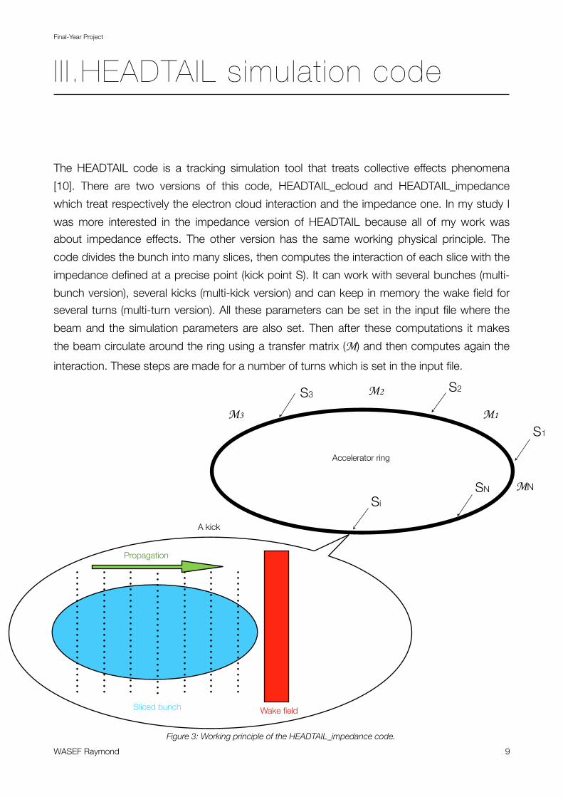
I I I.HEADTAIL simulation code
The HEADTAIL code is a tracking simulation tool that treats collective effects phenomena
[10]. There are two versions of this code, HEADTAIL_ecloud and HEADTAIL_impedance
which treat respectively the electron cloud interaction and the impedance one. In my study I
was more interested in the impedance version of HEADTAIL because all of my work was
about impedance effects. The other version has the same working physical principle. The
code divides the bunch into many slices, then computes the interaction of each slice with the
impedance defined at a precise point (kick point S). It can work with several bunches (multi-
bunch version), several kicks (multi-kick version) and can keep in memory the wake field for
several turns (multi-turn version). All these parameters can be set in the input file where the
beam and the simulation parameters are also set. Then after these computations it makes
the beam circulate around the ring using a transfer matrix (M) and then computes again the
interaction. These steps are made for a number of turns which is set in the input file.
Final-Year Project
WASEF Raymond 9
S1
S3
SN
M1
M2
M3
MN
Wake field
Figure 3: Working principle of the HEADTAIL_impedance code.
Sliced bunch
Si
Propagation
Accelerator ring
A kick

An example of the input file is given in Appendix, where one can find several beam parame-
ters like the energy, the tune and the chromaticity. There are also optics parameters like the
beta function, sextupoles strength and octupoles current (the current powering the octupoles
and which is directly linked to its magnetic field strength), as well as simulation parameters
like the number of turns, number of slices and memory of the wake.
The output of HEADTAIL has many files; the one which is interesting for this study is the one
with the "_prt.dat" extension. This file has 22 columns. The most important of them for this
study is the first one which is the time and the second one which is the average horizontal
position. The other columns contain the other average positions, the emittances, momentum,
etc.
This "_prt.dat" file is one of the complications I met in this work because it is huge (≈100Mb)
which limited the number of simultaneous simulations because of the account storage ca-
pacity I was using.
Other important outputs are the "_trk.dat" and the "_hdtl.dat"; the first one contains the wake
function used by HEADTAIL and the second one contains the average postion of the slices
along the bunch which allows the user to see the coherent motion of the bunch.
Final-Year Project
WASEF Raymond 10

j
IV. LHC simulations
After defining the parameters needed in the third section, I can now define exactly the objec-
tive of my work. The main idea is to benchmark HEADTAIL against theory from a stability
point of view. There are four different outputs which will be considered in this study; the tune-
shift that can be obtained from simulation and from theory, and the stabilizing octuple current
also from both of them. The benchmark between HEADTAIL, theory and experiment has al-
ready been done on several aspects of beam instability. However, reproducing the stability
diagram using HEADTAIL has never been done, and that's what makes the motivation of this
work. So the main objective of this work is for a given stability diagram (current and trans-
verse distribution defined), finding several points on the stability curve using theory, then
HEADTAIL simulations are made to try to reproduce the curve using HEADTAIL.
First of all, I simulated the case of the LHC at 3.5 TeV, single bunch, linear bucket, 115 10⁹ particle per bunch, horizontal chromaticity 6 and only the dipolar component of the LHC im-
pedance. The input file of this simulation is in Appendix for more details about the parameters
of this simulation. The objective of this work is to reproduce the stability diagram, so the best
attitude to have is to try to be as simple as possible to separate complications. That's why
this first simulation and also all the following ones were made only to study the horizontal
plane (chromaticity in the vertical one is 0 as well as the impedance) and considering only the
dipolar component of the impedance.
Using Sacherer's formula (4) I computed the tune-shift for this case, which gave
. This value is compared to the one given by HEADTAIL.
In the HEADTAIL output files one cannot get the tune-shift directly, so a step of post-
processing of the outputs is necessary. To get the real tune-shift, a fast Fourier transform was
made on the horizontal average position of the beam. Then to get the imaginary part of the
tune-shift, an exponential fit of the average horizontal position is required to get the rise time
(τ) which is directly linked to the imaginary part of the tune-shift through the following relation:
with Ω0: the revolution angular frequency
Final-Year Project
WASEF Raymond 11
(6)

The average horizontal position is plotted in Figure 4 as well as the average displacement of
the slices of the bunch over 20 turns (small figure). It can be easily seen that the absolute
value of the instability mode is 1 and after an exponential fit, the rise-time is 4.02s which gives
an imaginary part of .
After doing a fast Fourier transform (FFT) over this average horizontal position, I obtained the
values of Figure 5.
Final-Year Project
WASEF Raymond 12
3 different fits with 3.9 ; 4 and 4.1 as time constant
t (s)
x (m)
Figure 4: Exponential fit of the average horizontal position of the beam
Mode 1
Figure 5: FFT of the average position (horizontal axis ΔQ/Qs, vertical one the FFT amplitude)
x (m)
Slice number

j
j
In Figure 5 the horizontal axis is ΔQ/Qs and on the vertical one the amplitude of the FFT. One
can clearly see that the unstable mode is m=-1 mode and its real tune-shift is
.
Sacherer’s formula gives and the HEADTAIL simulation gives
. There is only 7% error on the imaginary part while there is almost a
factor 1.8 on the real part. This result is very satisfactory since one finds the tune-shift within
less than a factor 2 using a quite simple and approximated formula. One can notice this by
comparing the computation time of each one. For Sacherer, it was less than 20 minutes,
while a HEADTAIL simulation of 200 000 turns (less than 18s in the LHC) takes more or less 5
days (without any post-processing).
The tune-shift value was the first comparison between HEADTAIL and theory (Sacherer). Now
the second approach is to put both of the tune-shifts on a diagram where the horizontal axis
is the real tune-shift and the vertical one is the opposite of its imaginary part, we obtain two
points. Then using the dispersion equation (5), the stability diagram can be plotted for differ-
ent transverse distributions and octupoles currents. The idea then is to take a distribution,
then to change the octupoles current until finding the current for which the point is exactly on
the curve (stability limit). When the octupoles current increases, the area under the curve in-
creases, meaning that the stability area increases. For each current there are two different
curves; one of them is for the positive current and the other is for the negative one, because
the stability limit for the same absolute value of a current, is different. The stability diagram
also depends on the transverse distribution of the bunch; here I compare a Gaussian one to
a quasi-parabolic one [8]. One can already expect that the Gaussian should be more stable
so needs less current because it assumes an infinite distribution where the tails can absorb a
part of the energy. While the quasi-parabolic one underestimates the stability (needs more
current) because the LHC collimators are set at 6σ (the quasi-parabolic extends to 3.2σ).
Doing this scan of octupoles current for a given distribution, one can get the theoretical stabi-
lizing current (the one given by the stability diagram), then it is to be compared to the simu-
lated one which is given by HEADTAIL. The one given by HEADTAIL is obtained by simulating
several cases with different octupoles current and plotting the average horizontal position.
When the position is stable, it means that the stabilizing current is less than the one used.
When it is unstable, it means that it needs more current (in absolute value). This scan of oc-
tupoles current gives then a range of the simulated stabilizing current which can be com-
pared to the one from the stability diagram.
Final-Year Project
WASEF Raymond 13

Stability diagrams
-16 A
+26.5A
-37 A
+31A
Gaussian distribution Quasi-Parabolic distribution
HEADTAIL: between -5 and -10A
HEADTAIL: between +10 and +15A
HDTL tune-shift Sacherer tune-shift
In Figure 6 I did a scan of the octupoles current and I found for the LHC tune-shift given by
the HEADTAIL simulations, a stabilizing current of -16A (red curve) and +26.5A (blue curve)
for a Gaussian distribution. While for the quasi-parabolic one, it was higher as I expected,
-37A and +31A. In all the following cases I will just use the Gaussian distribution since HEAD-
TAIL uses a Gaussian distribution too.
Then I launched an intensity scan using HEADTAIL and I obtained the following results.
Final-Year Project
WASEF Raymond 14
Negative current
Figure 6: Stability diagram for the LHC for 2 different distributions and both of the current signs.
Figure 7: Average horizontal position for different octupoles currents: 0A (red), -5A (green) and -10A (blue).
t (s)
x (m)
Re(ΔQ)
-Im(ΔQ)
Re(ΔQ)
-Im(ΔQ)
Re(ΔQ)
-Im(ΔQ)
Re(ΔQ)
-Im(ΔQ)
Positive current

Final-Year Project
WASEF Raymond 15
Figure 7: Average horizontal position for different octupoles currents: -10A (red), -15A (green) and -30A (blue).
Figure 8: Average horizontal position for different octupoles currents: 0A (red), 5A (green), 10A (blue) and 15A (magenta)
Figure 9: Average horizontal position for different octupoles currents: 15A (red), 20A (green) and 50A (blue).
t (s)
x (m)
t (s)
x (m)
t (s)
x (m)

The HEADTAIL current scan gave a negative stabilizing current between -5A and -10A, and a
positive one between +10A and +15A. First of all, this result is confirming the fact that there is
a shift between the positive and the negative current and it confirms that for this given tune-
shift it is more efficient to stabilize with a negative current. There is a factor 2 between the two
approaches. It could be an error in the implementation of the code, in the physics or a real
difference between the stability diagram and HEADTAIL.
A first hypothesis was that the instability appears later in time, then we could not notice it in
the previous simulations. For example when I first did the simulations I tried many different
configurations. One of them was the linear and the non linear bucket for which I noticed that
with a non-linear bucket the instability appears much later (Figure 10.1). So as a first test I
tried to simulate the same case but over 500 000 turns instead of 200 000 (Figure 10.2).
We notice on Figure 10.2 that it is not a late appearance of the instability. The beam is still
stable after 500 000 turns, the difference comes then from another reason.
Final-Year Project
WASEF Raymond 16
11
Linear bucket 200k turns +15A
Non-linear bucket 200k turns 0A
Non-linear bucket 500k turns 0A
Figure 10.1: Average horizontal position for 3 different settings. 200 000 turns linear bucket at 15A (blue), 200 000 turns
non-linear bucket at 0A (green) and 500 000 turns non-linear bucket with 0A (red)
Figure 10.2: Average horizontal position for a 500 000 turns linear bucket with +15A
t (s)
x (m)
t (s)
0 5 10 15 20 25 30 35 40 45
2e-6
1.5e-6
1e-6
5e-7
0
-5e-7
-1.5e-6
-2e-6
4e-7
3e-7
2e-7
1e-7
0
-1e-7
-2e-7
-3e-7
-4e-7
-5e-7
x (m)

(7)
V. Scan of the stabil ity diagram
To avoid wasting time, especially since the simulations take a very long time, I continued the
project keeping in mind that there is a factor 2 to try to justify later.
At this stage of the internship, I did several simulations and a comparison with theory, but the
main goal to reach was to scan the stability diagram.
To be able to scan the stability diagram I had to change the impedance so that I could find
other tune-shifts which are exactly on the same stability curve.
A first trial was to simulate the LHC again but without collimators and then try to change the
beam intensity and try to find another point on the curve. But this wasn't successful because
I couldn't reach the stability curve using this model.
The second idea of impedance was the resonator impedance. In this model the transverse
impedance is written as following [4]:
Where, (ωr) is the resonance angular frequency, (Q) the quality factor and (R⊥) is the shunt
impedance.
Final-Year Project
WASEF Raymond 17
ω (s-¹)
Im(Z)
Re(Z)
h₁₁*5E27 (s²)
(Ω/m)
(Ω/m)
Figure 11: Example of a resonator with R⊥=17.5MΩ/m,Q=1 and f =0.64GHz. Thereal part of the impedance (blue curve),
imaginary part of impedance (red curve), h₁₁ (black curve)

Sacherer for LHC dipolar impedance only
HDTL for LHC dipolar impedance only
R=7.1M!/m, Q=0.5 f =0.75GHz
R=17.5M!/m, Q=1 f =0.64GHz
R=17.5M!/m, Q=1 f =0.6GHz
R=17.5M!/m, Q=2 f =0.6GHz
R=22.5M!/m, Q=1 f =0.1GHz
By changing the three parameters, I tried to scan the stability diagram at -24.8A which also
passes by the Sacherer tune-shift for LHC mode simulated in the previous section. After the
scan I obtained the following Figure 12:
In Figure 12 the blue curve is plotted to show the shift between the positive and negative oc-
tupoles current, even though it is useless in this plot. The tune-shifts obtained for these im-
pedances are given by Sacherer's formula; that's why when I chose a current I just took
-24.8A (passing by Sacherer’s tune-shift of the LHC) and not -16A (passing by the HEADTAIL
tune-shift of the LHC).
After HEADTAIL simulations, I found a very strange result (Figure 13). The result was so
strange that I had to check the reliability of every step of the analysis.
The first verification I did was to check if the slicing of the bunch was small enough to repro-
duce the wake field as it should be, because if the slices are too big the wake field will be de-
formed. The transverse wake function (G) is given by the following relation [4]:
Final-Year Project
WASEF Raymond 18
Figure 12: Scan of the stability diagram at -24.8A
Re(ΔQ)
-Im(ΔQ)
with:
(8)

Comparing the wake field given by Eq. (8) and the wake field used and fitted by HEADTAIL
(output file with the extension "_trk.dat") I obtained the results Figure 14.
Final-Year Project
WASEF Raymond 19
x: HDTL
o: Sacherer
Figure 13: Simulated scan of the stability diagram at -24.8A
Re(ΔQ)
-Im(ΔQ)
R=17.5M!/m, Q=1 f =0.64GHz R=17.5M!/m, Q=1 f =0.6GHz
R=17.5M!/m, Q=2 f =0.6GHz R=22.5M!/m, Q=1 f =0.1GHz
Theory
HDTL
Figure 14: Comparing the wake function from HEADTAIL and theory
G (V/C.m²)
t (s)
G (V/C.m²)
t (s)
G (V/C.m²)
t (s)
G (V/C.m²)
t (s)

The wake fields are exactly the same, so the problem is not a problem of slicing. Then I tried
to check the accuracy of the tune-shifts calculated from HEADTAIL. First of all, I tried to use
SUSSIX which is a computer code for frequency analysis [11]. The result of SUSSIX was al-
most the same as the FFT. Then I checked the imaginary part of the tune shift. The first time I
was fitting the horizontal position, I was using a code which fits the logarithm value of the
module of the horizontal position. This time I used another code that fits directly the curve
with an exponential; the result was the same (3% difference in the worst case) which means
that the problem is not a problem of the HEADTAIL post-processing. Then I tried to check the
accuracy of the code that compute Sacherer’s formula. In this code the condition to stop
summing terms is that the ratio of the first abandoned term and the sum is less than
. Then I put this condition to which gave me exactly the same result. So we
could think that there is no sum error in the Sacherer formula, but further investigations are
needed.
At this stage I found an error in my implementation of the Sacherer formula. After I corrected
this error, the Sacherer tune-shift changed. It has now a better real tune-shift compared to
the HEADTAIL one but the imaginary part is still completely different from the HEADTAIL one.
This means that now the points that were supposed to be on the stability edge changed their
value and are not on the stability edge anymore. However, it is still important to solve the
problem of the huge difference between HEADTAIL and Sacherer even if the points are not
on the curve because anyway I will have to use Sacherer’s formula to scan the curve again.
To check which of the values is wrong, I used the MOSES code (MOde coupling Single
bunch instability in an Electron Storage ring) which is a code that computes the tune-shift and
the transverse mode coupling threshold from a resonator impedance [12]. The advantage of
this code is that it is very quick and very easy. For the five points I compared MOSES,
Sacherer and HEADTAIL (without octupoles) and I obtained the following results:
Final-Year Project
WASEF Raymond 20
MOSES
HDTL
Sacherer
R=7.1M!/m, Q=0.5 f =0.75GHz
Figure 15: Comparing HEADTAIL, MOSES and Sacherer for the first scan point (without octupoles)
Re(ΔQ)
-Im(ΔQ)

It can be easily noticed that HEADTAIL and MOSES are in good agreement while Sacherer’s
formula always gives a very different imaginary part.
The error is then most probably coming from the Sacherer formula. The first thing to check is
the implementation. Dr. Elias Metral checked the values with his own implementation and he
found results with more or less 40% error compared to the HEADTAIL value. Which is ex-
pected because Sacherer’s formula is an approximated formula that should be valid within a
factor 2. Since I already checked many times the implementation I am using and I didn't find
any error, I wrote another one using a trapeze integral instead of a sum. This time I found
much better results (in the worst case 66% error compared to HEADTAIL value, see Figure
17). So we could think now that there is indeed a numerical problem with the first method
since I am using exactly the same parameters but just a different way to sum; investigations
are ongoing.
Final-Year Project
WASEF Raymond 21
MOSES
HDTL
Sacherer
MOSES
HDTL
Sacherer
MOSES
HDTL
Sacherer
MOSES
HDTL
Sacherer
R=17.5M!/m, Q=1 f =0.64GHz R=17.5M!/m, Q=1 f =0.6GHz
R=17.5M!/m, Q=1 f =0.6GHz R=22.5M!/m, Q=1 f =0.1GHz
Figure 16: Comparing HEADTAIL, MOSES and Sacherer for the four other scan points
Re(ΔQ)
-Im(ΔQ)
Re(ΔQ)
-Im(ΔQ)
Re(ΔQ)
-Im(ΔQ)
Re(ΔQ)
-Im(ΔQ)
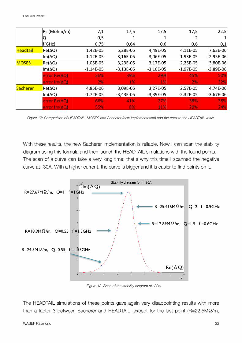
With these results, the new Sacherer implementation is reliable. Now I can scan the stability
diagram using this formula and then launch the HEADTAIL simulations with the found points.
The scan of a curve can take a very long time; that's why this time I scanned the negative
curve at -30A. With a higher current, the curve is bigger and it is easier to find points on it.
The HEADTAIL simulations of these points gave again very disappointing results with more
than a factor 3 between Sacherer and HEADTAIL, except for the last point (R=22.5MΩ/m,
Final-Year Project
WASEF Raymond 22
!! "#!$%&'()(*! +,-! -+,.! -+,.! -+,.! //,.!
!! 0! 1,.! -! -! /! -!
!! 2$345*! 1,+.! 1,67! 1,6! 1,6! 1,-!
489:;9<=! "8$>0*! -,7/?@1.! .,/A?@1.! 7,7B?@1.! 7,--?@1.! +,6C?@16!
!! D($>0*! @-,-/?@1.! @C,-6?@1.! @C,16?@1.! @-,BC?@1.! @/,B.?@16!
%EF?F! "8$>0*! -,1.?@1.! C,/C?@1.! C,-+?@1.! /,/.?@1.! C,A1?@16!
!! D($>0*! @-,-7?@1.! @C,-C?@1.! @C,-1?@1.! @-,B+?@1.! @C,AB?@16!
!! 8GG&G!"8$>0*! /6H! CBH! /BH! 7.H! .1H!
!! 8GG&G!D($>0*! /H! -H! -H! /H! C/H!
F9I'8G8G! "8$>0*! 7,A.?@16! C,1B?@1.! C,/+?@1.! /,.+?@1.! 7,+7?@16!
!! D($>0*! @-,+/?@1.! @C,7C?@1.! @C,CB?@1.! @/,C/?@1.! @C,6+?@16!
!! 8GG&G!"8$>0*! 66H! 7-H! /+H! CAH! CAH!
!! 8GG&G!D($>0*! ..H! AH! --H! /1H! /7H!
Figure 17: Comparison of HEADTAIL, MOSES and Sacherer (new implementation) and the error to the HEADTAIL value
R=24.5M!/m, Q=0.55 f =1.55GHz
R=18.9M!/m, Q=0.55 f =1.3GHz
R=27.67M!/m, Q=1 f =1GHz
R=25.415M!/m, Q=2 f =0.9GHz
R=12.89M!/m, Q=1.5 f =0.6GHz
Re("Q)
-Im("Q)
Figure 18: Scan of the stability diagram at -30A

R=7.1M!/m, Q=0.5 f =0.75GHz
R=17.5M!/m, Q=2 f =0.6GHz R=22.5M!/m, Q=1 f =0.1GHz
R=17.5M!/m, Q=1 f =0.64GHz R=17.5M!/m, Q=1 f =0.6GHz
The current of the simulated beam
Figure 19: Mode coupling threshold for the 5 points, the simulated beam current is 0.207 mA (in dotted red curve).
Q=1 f =0.1GHz). When I checked with MOSES these five points I found results very close to
HEADTAIL. The important thing I noticed was that the mode coupling threshold was much
higher for the last point than all the others. That's most probably why it is the only point for
which I got an agreement between HEADTAIL and Sacherer, because Sacherer’s formula
supposes that there is no mode-coupling and that every mode can be treated seperatly.
Final-Year Project
WASEF Raymond 23

Figure 19 shows the mode coupling threshold for the different points (in the simulation case
the beam intensity is 0.207 mA), the horizontal axis is the beam intensity and the vertical one
is the real tune-shift. It is clear that in the case of the last point the threshold is much higher
than the other cases (mode coupling is when 2 different tune-shifts become the same).
To avoid mode coupling I had to reduce the octupoles current. I chose then to scan a stability
diagram at -10A. There was a trade-off between high octupoles current to have bigger tune-
shifts, so faster instability (for the simulation time); and low octupoles current to have small
tune-shifts and be far away from mode-coupling.
This time I checked the threshold of Mode coupling and verified that it was at least five times
higher than the beam intensity (0.2 mA).
With the HEADTAIL simulations I obtained less than a factor 2 difference between HEADTAIL
and Sacherer. This time I tried to change the number of turns over which I do the FFT and
over which I fit the average position, so that I can estimate a range of the tune-shift that takes
into account at least a part of the post-processing errors; but also can introduce errors if
there are some damping during the instability. For example, in the fourth plot of the Figure 21
the imaginary part has a huge error bar. The fit should be the envelope of both of the rising
parts, when the number of turns is reduced the fit is not very good, but if one considers all
the simulation turns, there is less than a factor 2 error (I took in account this effect because
maybe someone else will do the same simulation but with different number of turns). The re-
sults of the points are given in Figure 21. Then I launched an octupoles current scan with
Final-Year Project
WASEF Raymond 24
R=7.2M!/m, Q=0.55 f =1.5GHz
R=5.9M!/m, Q=0.52 f =1.25GHz
R=5.62M!/m, Q=0.5 f =1.1GHz R=4M!/m, Q=0.51 f =0.8GHz
R=3.68M!/m, Q=0.55 f =0.75GHz
R=3.15M!/m, Q=0.51 f =0.5GHz
-Im(ΔQ)
Figure 20: Scan of the stability diagram at -10A

HEADTAIL. As one can see on Figure 22 to Figure 33, all the points stabilize between -4A
and -6A. Which brings the factor 2 for the second time.
Final-Year Project
WASEF Raymond 25
R=7.2M!/m, Q=0.55 f =1.5GHz R=5.9M!/m, Q=0.52 f =1.25GHz
R=5.62M!/m, Q=0.5 f =1.1GHz R=4M!/m, Q=0.51 f =0.8GHz
R=3.68M!/m, Q=0.55 f =0.75GHz R=3.15M!/m, Q=0.51 f =0.5GHz
Sacherer
HEADTAIL range
Sacherer
HEADTAIL range
Sacherer
HEADTAIL range
HEADTAIL range
Sacherer
HEADTAIL range
Sacherer
HEADTAIL range
Sacherer
Figure 21: Results for the scanned curve at -10A (Sacherer tuner-shift in dark blue, a range of the HEADTAIL tune-shift in light blue)
Re(ΔQ)
-Im(ΔQ)
Re(ΔQ)
-Im(ΔQ)
Re(ΔQ)
-Im(ΔQ)
Re(ΔQ)
-Im(ΔQ)
Re(ΔQ)
-Im(ΔQ)
Re(ΔQ)
-Im(ΔQ)

Final-Year Project
WASEF Raymond 26
R=7.2M!/m, Q=0.55 f =1.5GHz R=7.2M!/m, Q=0.55 f =1.5GHz
Figure 22: Average horizontal position for different octupoles currents
0A (red), -2A (green), -4A (blue) and -6A (magenta)
Figure 23: Average horizontal position for different octupoles currents
-4A (red), -6A (green) and -8A (blue)
Figure 24: Average horizontal position for different octupoles currents
0A (red), -2A (green) and -4A (blue).
Figure 25: Average horizontal position for different octupoles currents
-4A (red), -6A (green) and -8A (blue)
R=5.62M!/m, Q=0.5 f =1.1GHz R=5.62M!/m, Q=0.5 f =1.1GHz
turns
x (m)
turns
x (m)
turns
x (m)
turns
x (m)

Final-Year Project
WASEF Raymond 27
Figure 26: Average horizontal position for different octupoles currents
0A (red), -2A (green) and -4A (blue).
Figure 27: Average horizontal position for different octupoles currents
-4A (red), -6A (green) and -20A (blue)
R=5.9M!/m, Q=0.52 f =1.25GHz R=5.9M!/m, Q=0.52 f =1.25GHz
Figure 28: Average horizontal position for different octupoles currents
0A (red), -2A (green) and -4A (blue).
Figure 29: Average horizontal position for different octupoles currents
-4A (red), -6A (green) and -20A (blue)
R=4M!/m, Q=0.51 f =0.8GHz R=4M!/m, Q=0.51 f =0.8GHz
turns
x (m)
turns
x (m)
turns
x (m)
turns
x (m)

Final-Year Project
WASEF Raymond 28
Figure 30: Average horizontal position for different octupoles currents
0A (red), -2A (green) and -4A (blue).
Figure 31: Average horizontal position for different octupoles currents
-4A (red), -6A (green) and -10A (blue)
R=3.68M!/m, Q=0.55 f =0.75GHz R=3.68M!/m, Q=0.55 f =0.75GHz
Figure 32: Average horizontal position for different octupoles currents
0A (red), -2A (green) and -4A (blue).
Figure 33: Average horizontal position for different octupoles currents
-4A (red), -6A (green) and -10A (blue)
R=3.15M!/m, Q=0.51 f =0.5GHz
R=3.15M!/m, Q=0.51 f =0.5GHz
turns
x (m)
turns
x (m)
turns
x (m)
turns
x (m)

This factor 2 is still unexplained but there are three possible reasons:
• An error in the implementation of the stability diagram
• An error in the computation of the action variables coefficients in HEADTAIL.
• The theory is not precise
These three ideas are being investigated at the moment.
The same method is now applied to scan the positive curve and to see whether it is the same
factor (almost 2) in both cases or not. For the moment, I already have the points on the curve
(Figure 34), I checked their mode coupling threshold and launched their HEADTAIL simula-
tions with and without octupoles.
For the last two scans (-10A and +10A), I changed the output of HEADTAIL to get rid of all
the outputs I don't need which extremely reduced the size of the outputs and allowed me to
make more simultaneous simulations. That's the main reason why the current scan step in
HEADTAIL is currently only 2A.
Final-Year Project
WASEF Raymond 29
Re(ΔQ)
-Im(ΔQ)
Figure 34: Scan of the stability diagram at +10A
R=4.52M!/m, Q=0.6 f =1.4GHz
R=4.62M!/m, Q=0.7 f =1.1GHz
R=4.42M!/m, Q=0.6 f =0.9GHz
R=5.85M!/m, Q=0.6 f =0.4GHz

VI. Conclusion
The goal of this project was mainly to benchmark theory against simulations. The theory here
was Sacherer's formula and the stability diagram while the simulation code used was HEAD-
TAIL_impedance. This benchmarking was never done before and it was really interesting to
check that what is important is the stability curve, as two beams with totally different complex
tune-shifts need the same current to be stabilized. It is also amazing to see how a simple
formula like the Sacherer one is very powerful and can give a result within a factor 2 in 10
minutes (compared to a simulation that takes weeks). After facing a lot of problems in imple-
mentation, theory, simulation, storage capacity, etc. I finally managed to get a scan of the
curve that works and that gives a tune-shift and a stabilizing current which are within a factor
2 compared to theory. These results show also how the HEADTAIL code is a reliable and a
powerful code.
This project began on the 2nd of May and will continue until the 17th of September. That's
why there is still some work to be completed like the positive curve and I probably will try to
change the distribution function in HEADTAIL and try to see its effect on the stability diagram
as predicted in Ref. [8,9].
This internship was a great opportunity for me to discover instabilities and collective effects.
Even if my work was focused on a particular study case, I attended many meetings and talks
where I learned many things especially that it is very easy to learn new things when one
doesn't know the field at all.
Final-Year Project
WASEF Raymond 30
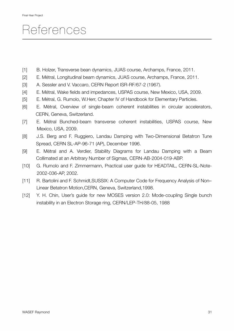
References
[1] B. Holzer, Transverse bean dynamics, JUAS course, Archamps, France, 2011.
[2] E. Métral, Longitudinal beam dynamics, JUAS course, Archamps, France, 2011.
[3] A. Sessler and V. Vaccaro, CERN Report ISR-RF/67-2 (1967).
[4] E. Métral, Wake fields and impedances, USPAS course, New Mexico, USA, 2009.
[5] E. Métral, G. Rumolo, W.Herr, Chapter IV of Handbook for Elementary Particles.
[6] E. Métral, Overview of single-beam coherent instabilities in circular accelerators,
CasddCERN, Geneva, Switzerland.
[7] E. Métral Bunched-beam transverse coherent instabilities, USPAS course, New
MexicoMexico, USA, 2009.
[8] J.S. Berg and F. Ruggiero, Landau Damping with Two-Dimensional Betatron Tune
Spr Spread, CERN SL-AP-96-71 (AP), December 1996.
[9] E. Métral and A. Verdier, Stability Diagrams for Landau Damping with a Beam
C Collimated at an Arbitrary Number of Sigmas, CERN-AB-2004-019-ABP.
[10] G. Rumolo and F. Zimmermann, Practical user guide for HEADTAIL, CERN-SL-Note-
vvvvvG2002-036-AP, 2002.
[11] R. Bartolini and F. Schmidt,SUSSIX: A Computer Code for Frequency Analysis of Non–
Linear Betatron Motion,CERN, Geneva, Switzerland,1998.
[12] Y. H. Chin, User’s guide for new MOSES version 2.0: Mode-coupling Single bunch
LAWWinstability in an Electron Storage ring, CERN/LEP-TH/88-05, 1988
Final-Year Project
WASEF Raymond 31

Appendix: Example of a LHC HEADTAIL input f i le
Flag_for_bunch_particles_(1->protons_2->positrons_3&4->ions): 1Number_of_particles_per_bunch: 115e+9 Horizontal_beta_function_at_the_kick_sections_[m]: 65.9756 Vertical_beta_function_at_the_kick_sections_[m]: 71.5255Bunch_length_(rms_value)_[m]: 0.056Normalized_horizontal_emittance_(rms_value)_[um]: 3.75Normalized_vertical_emittance_(rms_value)_[um]: 3.75Longitudinal_momentum_spread: 0.00012Synchrotron_tune: 0.0028911Momentum_compaction_factor: 0.0003225Ring_circumference_length_[m]: 26658.883Relativistic_gamma: 3730.26Number_of_kick_sections: 1Number_of_turns: 200000Multiplication_factor_for_pipe_axes 10Multiplication_factor_for_pipe_axes 10Longitud_extension_of_the_bunch_(+/-N*sigma_z) 2.Horizontal_tune: 64.31Vertical_tune: 59.32Horizontal_chromaticity: 6Vertical_chromaticity: 0Flag_for_synchrotron_motion: 1Number_of_macroparticles: 1000000Number_of_bunches: 1Number_of_slices_in_each_bunch: 500Spacing_between_consecutive_bunches_centroids_[m]: 7.5Switch_for_bunch_table: 0Switch_for_wake_fields: 1Switch_for_pipe_geometry_(0->round_1->flat): 9Number_of_turns_for_the_wake: 10Res_frequency_of_broad_band_resonator_[GHz]: 1.0Transverse_quality_factor: 1.Transverse_shunt_impedance_[MOhm/m]: 0.Res_frequency_of_longitudinal_resonator_[MHz]: 200Longitudinal_quality_factor: 140.Longitudinal_shunt_impedance_[MOhm]: 0.0Conductivity_of_the_resistive_wall_[1/Ohm/m]: 1.e6Length_of_the_resistive_wall_[m]: 69110.Switch_for_beta: 0Switch_for_wake_table: 6Flag_for_the_tune_spread_(0->no_1->space_charge_2->random): 0Flag_for_the_sc-rotation(0->local_centroid_1->bunch_centroid): 0
Final-Year Project
WASEF Raymond 32
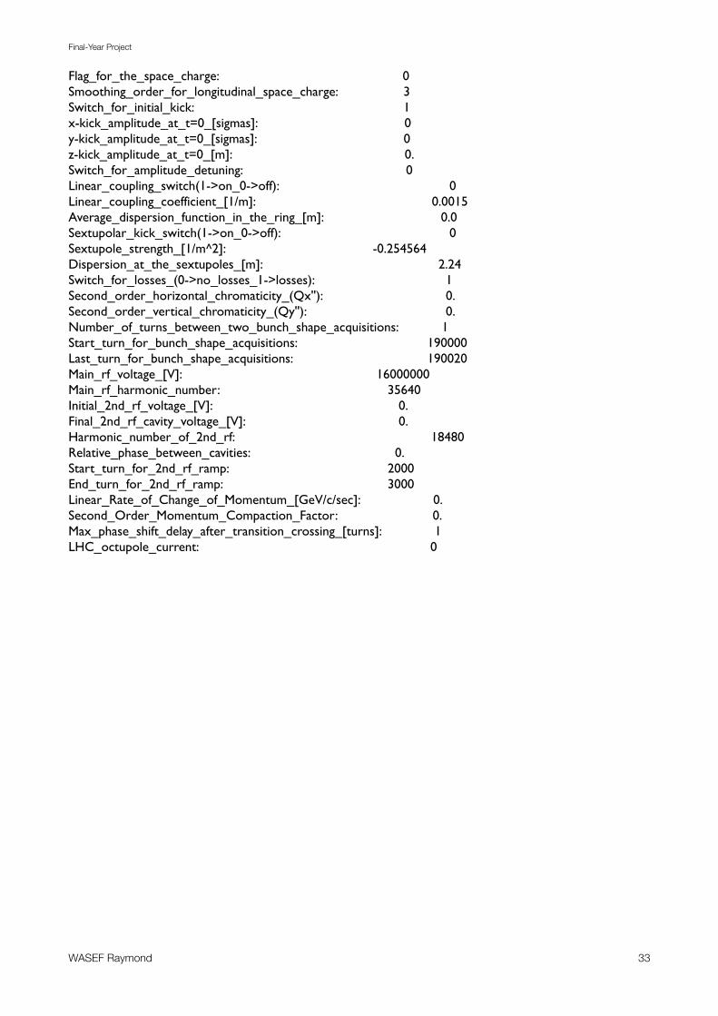
Flag_for_the_space_charge: 0Smoothing_order_for_longitudinal_space_charge: 3Switch_for_initial_kick: 1x-kick_amplitude_at_t=0_[sigmas]: 0y-kick_amplitude_at_t=0_[sigmas]: 0z-kick_amplitude_at_t=0_[m]: 0.Switch_for_amplitude_detuning: 0Linear_coupling_switch(1->on_0->off): 0Linear_coupling_coefficient_[1/m]: 0.0015Average_dispersion_function_in_the_ring_[m]: 0.0Sextupolar_kick_switch(1->on_0->off): 0Sextupole_strength_[1/m^2]: -0.254564Dispersion_at_the_sextupoles_[m]: 2.24Switch_for_losses_(0->no_losses_1->losses): 1Second_order_horizontal_chromaticity_(Qx''): 0.Second_order_vertical_chromaticity_(Qy''): 0.Number_of_turns_between_two_bunch_shape_acquisitions: 1Start_turn_for_bunch_shape_acquisitions: 190000Last_turn_for_bunch_shape_acquisitions: 190020Main_rf_voltage_[V]: 16000000Main_rf_harmonic_number: 35640Initial_2nd_rf_voltage_[V]: 0.Final_2nd_rf_cavity_voltage_[V]: 0.Harmonic_number_of_2nd_rf: 18480Relative_phase_between_cavities: 0.Start_turn_for_2nd_rf_ramp: 2000End_turn_for_2nd_rf_ramp: 3000Linear_Rate_of_Change_of_Momentum_[GeV/c/sec]: 0.Second_Order_Momentum_Compaction_Factor: 0.Max_phase_shift_delay_after_transition_crossing_[turns]: 1LHC_octupole_current: 0
Final-Year Project
WASEF Raymond 33

Summary
This internship was performed at European Organization for Nuclear Research (CERN) from
the 2nd of May to the 17th of September. It was about the collective effects and more
precisely impedances. The main goal of this project was to benchmark theory against a
simulation code called HEADTAIL; and try to reproduce the so called stability diagram.
First of all, I started with a simulation of the LHC but only with its dipolar component. The
results were satisfying; less than a factor 2 difference between theory and simulation. Then, I
scanned a curve of the stability diagram using Sacherer’s formula for different resonator
impedances. I also found satisfying results for an octupoles current of -10A. Since I still have
3 more weeks to continue the project, I already launched other simulations for an octupoles
current of +10A and I am also planing to change the transverse distribution of the beam in
HEADTAIL to see its effect on the stabilizing current.
This internship was a great opportunity to discover the world of collective effects and
impedances. It is one of the main motivations I had when I decided to continue working and
doing my PhD in this field.
Final-Year Project
WASEF Raymond 34

Résumé
Ce projet de fin d'études s’est déroulé à l’Organisation Européenne pour la Recherche
Nucléaire (CERN); du 2 mai 2011 jusqu’au 17 septembre 2011. Le travail effectué était
surtout dans le domaine des effets collectifs et plus précisément les impédances des
accélérateurs de particules. Le but principal du projet était de comparer la théorie et un code
de simulation appelé HEADTAIL, en essayant de retracer un diagramme de stabilité grâce à
HEADTAIL.
Tout d’abord, j’ai commencé par une simulation du LHC avec uniquement la composante
dipolaire de son impédance. Les résultats de cette simulation étaient satisfaisants avec moins
d’un facteur 2 de différence. Ensuite j’ai balayé la courbe de stabilité en utilisant la formule de
Sacherer pour différentes impédances de résonateur et avec -10A pour le courant des
octupoles. Les résultats de ces simulations étaient aussi en accord avec la théorie.
Actuellement, j’attends les résultats des simulations que j’ai faites pour la courbe avec un
courant dans les octupoles de +10A. Pendant les trois semaines qui me restent, je prévois de
changer la distribution transverse dans le code HEADTAIL pour voir son effet sur le
diagramme de stabilité.
Ce projet m’a permis de découvrir le domaine des effets collectifs; et a été une des
principales raisons de ma décision de faire ma thèse et de continuer de travailler dans le
domaine des effets collectifs.
Final-Year Project
WASEF Raymond 35