Embed Size (px)
Citation preview

FINAL VERSION IJCAI 2009 TUTORIAL
Version 4, July 13, 2009

Logical and Relational Learning
Luc De Raedt
An IJCAI 2009 Tutorial
ⓒ Luc De Raedt

What is Logical and Relational Learning ?
Inductive Logic
Programming
(Statistical) Relational Learning
Multi-Relational Data
Mining
Mining and Learning in Graphs
UNION of
They all study the same problem

The Problem
Learning from structured data, involving
• objects, and
• relationships amongst them
and possibly
• using background knowledge
Purpose of this talk
Relational learning is sometimes viewed as a new problem, but it has a long history
Emphasize the role of symbolic representations (graphs & logic) and knowledge
A modern view
• logic as a toolbox for machine learning
Overview of some of the available tools and techniques
Illustration of their use in some of our recent work

HistoryPhilosophy of Science: Carnap, Hume, Miller, Popper, Peirce, ...
AI & ML 60s-70s: Banerji, Plotkin, Vere, Michalski, ...
AI & ML 80s: Shapiro, Sammut, Muggleton, ...
ILP 90s: Muggleton, Quinlan, De Raedt, ...
SRL 00s: Getoor, Koller, Domingos, Sato, ...

OverviewPart I : Introduction
• MOTIVATION
• REPRESENTATIONS OF THE DATA
Part II : Logical and Relational Learning
• The LOGIC of LEARNING
• METHODOLOGY and SYSTEMS
Part III : Statistical Relational Learning
• LOGIC, RELATIONS and PROBABILITY
• RELATIONAL REINFORCEMENT LEARNING

Further Reading
Luc De Raedt
Logical and Relational Learning
Springer, 2008, 401 pages.
(should be on display at the Springer booth)

The MOTIVATION

Case 1: Structure Activity Relationship Prediction
O CH=N-NH-C-NH 2O=N
O - O
nitrofurazone
N O
O
+
-
4-nitropenta[cd]pyrene
N
O O-
6-nitro-7,8,9,10-tetrahydrobenzo[a]pyrene
NH
NO O-
+
4-nitroindole
Y=Z
Active
Inactive
Structural alert:
[Srinivasan et al. AIJ 96]
Data = Set of Small Graphs
General PurposeLogic Learning System
Uses and ProducesKnowledge

Using and Producing Knowledge
LRL can use and produce knowledge
Result of learning task is understandable and interpretable
Logical and relational learning algorithms can use background knowledge, e.g. ring structures, pathways, ...
and reason, induction, deduction, abduction, ...
Focus of Inductive Logic Programming

Case 2: The Robot Scientist
Nature 2004
REPORTSThe Automation of ScienceRoss D. King,1* Jem Rowland,1 Stephen G. Oliver,2 Michael Young,3 Wayne Aubrey,1 Emma Byrne,1 Maria Liakata,1 Magdalena Markham,1 Pinar Pir,2 Larisa N. Soldatova,1 Andrew Sparkes,1 Kenneth E. Whelan,1 Amanda Clare1
Science 2009
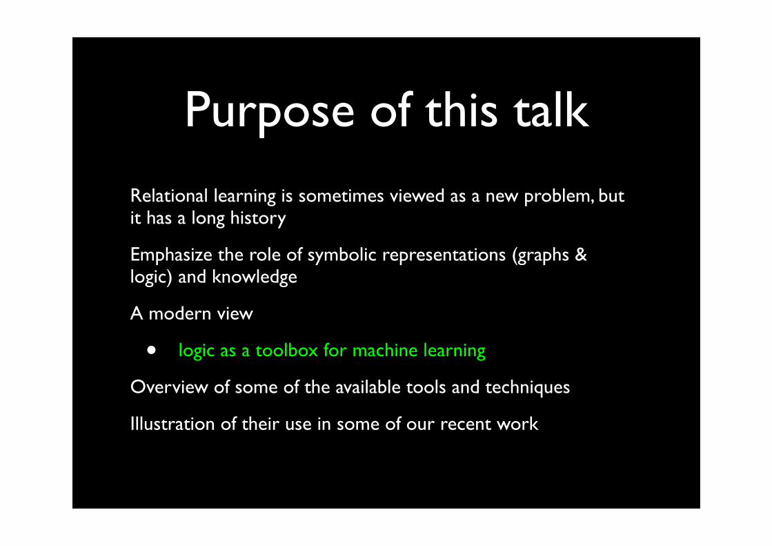
gene
protein
pathway
cellularcomponent
homologgroup
phenotype
biologicalprocess
locus
molecularfunction has
is homologous to
participates in
participates inis located in
is related to
refers tobelongs to
is found in
codes for
subsumes,interacts with
is found in
participates in
refers to
Case 3: Biological NetworksBiomine Database @ Helsinki
Data = Large (Probabilistic) Network
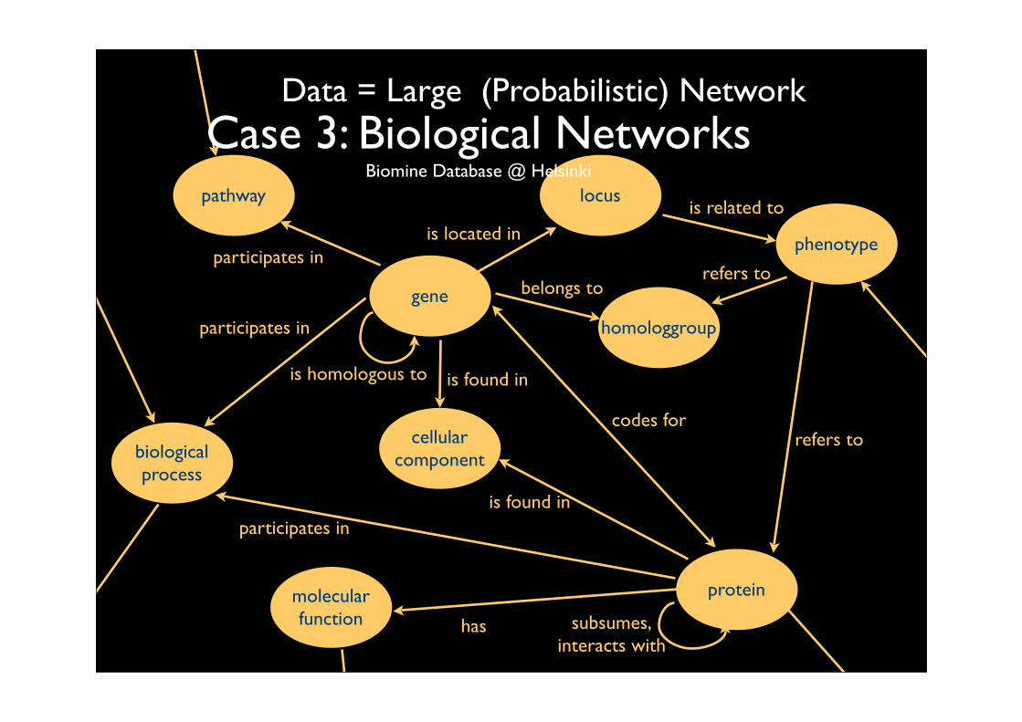
Network around Alzheimer Disease

presenilin 2Gene
EntrezGene:81751
Notch receptor processingBiologicalProcessGO:GO:0007220

-participates_in0.220
BiologicalProcess
Gene
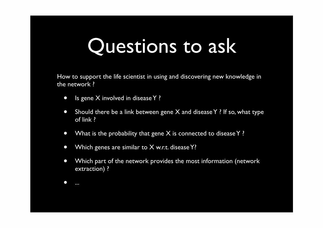
Questions to askHow to support the life scientist in using and discovering new knowledge in the network ?
• Is gene X involved in disease Y ?
• Should there be a link between gene X and disease Y ? If so, what type of link ?
• What is the probability that gene X is connected to disease Y ?
• Which genes are similar to X w.r.t. disease Y?
• Which part of the network provides the most information (network extraction) ?
• ...

Case 4: Evolving Networks
Travian: A massively multiplayer real-time strategy game
• Commercial game run by TravianGames GmbH
• ~3.000.000 players spread over different “worlds”
• ~25.000 players in one world[Thon et al. ECML 08]
World Dynamics
border
border
border
border
Alliance 2
Alliance 3
Alliance 4
Alliance 6
P 2
1081
8951090
1090
1093
1084
1090
915
1081
1040
770
1077
955
1073
8041054
830
9421087
786
621
P 3
744
748559
P 5
861
P 6
950
644
985
932
837871
777
P 7
946
878
864 913
P 9
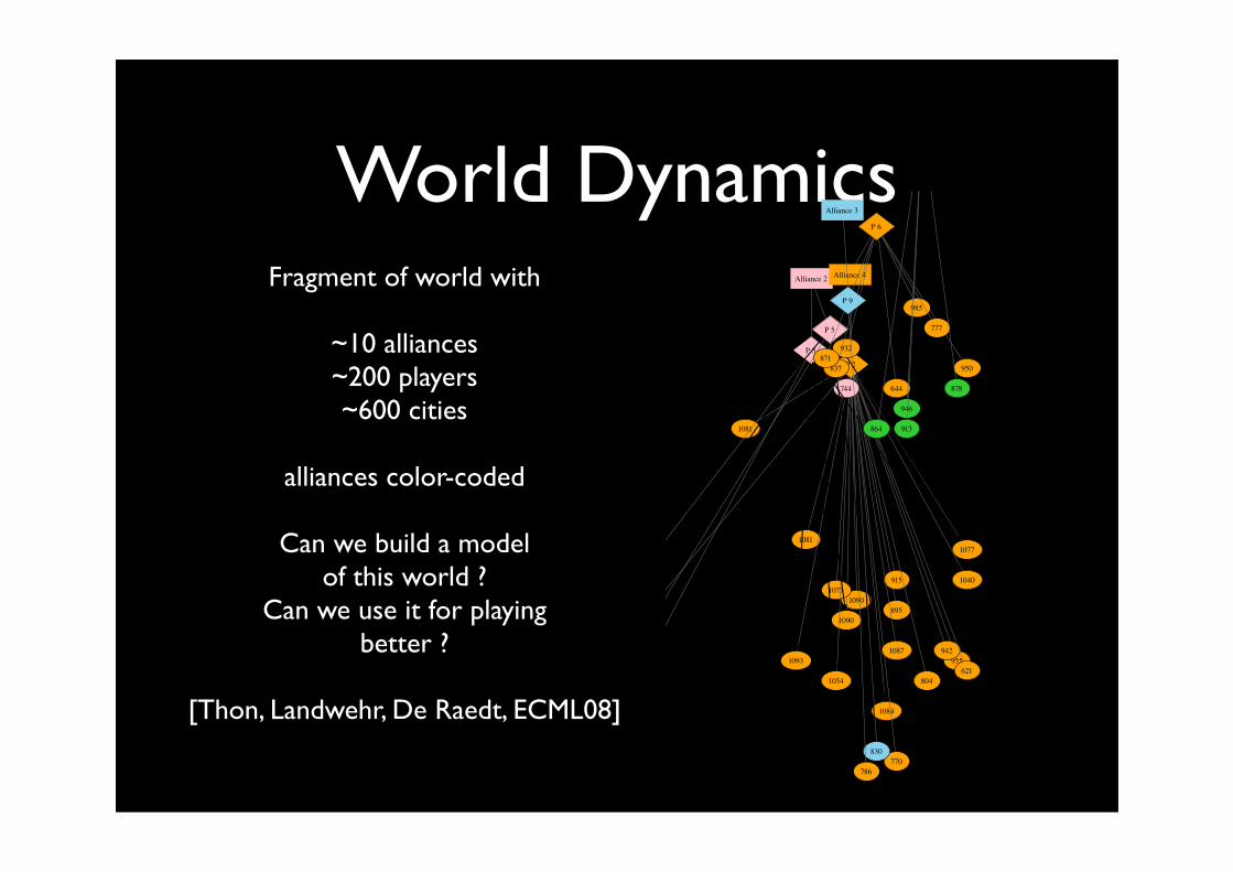
Fragment of world with
~10 alliances~200 players~600 cities
alliances color-coded
Can we build a modelof this world ?
Can we use it for playingbetter ?
[Thon, Landwehr, De Raedt, ECML08]

World Dynamics
border
border
border
border
Alliance 2
Alliance 4
Alliance 6
P 2
9041090
917
770
959
1073
820
762
9461087
794
632
P 3
761
961
1061
607
988
771
924
583
P 5
951
935
948
938
867
P 6
950
644
985
888
844875
783
P 7
946
878
864 913
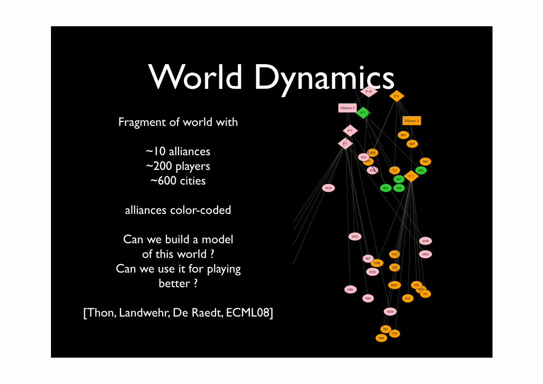
Fragment of world with
~10 alliances~200 players~600 cities
alliances color-coded
Can we build a modelof this world ?
Can we use it for playingbetter ?
[Thon, Landwehr, De Raedt, ECML08]
World Dynamics
border
border
border
border
Alliance 2
Alliance 4
Alliance 6
P 2
9181090
931
779
977
835
781
9581087
808
701
P 3
838
947
1026
1081
833
1002987
827
994
663
P 5
1032
1026
1024
1049
905
926
P 6
986
712
985
920
877
807
P 7
895
959
P 10
824
Fragment of world with
~10 alliances~200 players~600 cities
alliances color-coded
Can we build a modelof this world ?
Can we use it for playingbetter ?
[Thon, Landwehr, De Raedt, ECML08]

World Dynamics
border
border
border
border
Alliance 2
Alliance 4
Alliance 6
P 2
9231090
941
784
983
844
786
9661087
815
711
P 3
864
986
842
1032
1083
868
712
10021000
858
996
696
P 5
1039
1037
1030
1053
826
933
P 6
985
807
P 7
894
963
P 10
829
781828
Fragment of world with
~10 alliances~200 players~600 cities
alliances color-coded
Can we build a modelof this world ?
Can we use it for playingbetter ?
[Thon, Landwehr, De Raedt, ECML08]

World Dynamics
border
border
border
border
Alliance 2Alliance 4
Alliance 6
P 2
9381090
949
785
987
849
789
9761087
821
724
P 3
888
863
868
1040
1083
896
667
1005994
883
1002
742
P 5
1046
1046
1040
985
894
1058
879
938
921
807
P 6P 7
P 10
830
782829
Fragment of world with
~10 alliances~200 players~600 cities
alliances color-coded
Can we build a modelof this world ?
Can we use it for playingbetter ?
[Thon, Landwehr, De Raedt, ECML08]

World Dynamics
border
border
border
border
Alliance 2
Alliance 4
P 2
948
951
786
990
856
795
980
828
730
P 3898
803
860
964
1037
1085
925
689
10051007
899
1005
760
P 5
1051
1051
1040
860
774
1061
886
944
844
945
713
P 10
839
796838
Fragment of world with
~10 alliances~200 players~600 cities
alliances color-coded
Can we build a modelof this world ?
Can we use it for playingbetter ?
[Thon, Landwehr, De Raedt, ECML08]
Emerging Data Sets
In many application areas :
• vision, surveillance, activity recognition, robotics, ...
• data in relational format are becoming available
• use of knowledge and reasoning is essential
• in Travian -- ako STRIPS representation

GerHome Example
Action and Activity Learning
(courtesy of Francois Bremond, INRIA-Sophia-Antipolis)
http://www-sop.inria.fr/orion/personnel/Francois.Bremond/topicsText/gerhomeProject.html

Towards “Relational” Robotics ?
Robotics
• several lower level problems have been (more or less) solved
• time to bridge the gap between lower and higher level representations ?
[Kersting et al. Adv. Robotics 07]

The LRL Problem
Learning from structured data, involving
• objects, and relationships amongst them
• possibly using background knowledge and reasoning
Very often :
• examples are small graphs or elements of a large network (possibly evolving over time)
• many different types of applications and challenges

BASICS

BASICSlogic

The Representation Language
SQL
Prolog First Order Logic
Relational Calculi Entity-Relationship Model
Description Logic
OWL
Choice probably not that important though implementation & manipulation
Graphs

Logic: Syntaxclass(Book,Topic) :-
author(Book,Author), favorite-topic(Author,Topic).
the class of Book is Topic IF
the Book is written by Author AND
Topic is the favorite of the Author
favorite-topic(rowlings,fantasy)
the favorite topic of rowlings is fantasy
author(rowlings,harrypotter)
Variableconstant
predicate/relation
Fact(s)
Clause(s)

Logic: three viewsentailment/logical consequence
class(Book,Topic) :-
author(Book,Author), favorite-topic(Author,Topic)
favorite-topic(rowlings,fantasy).
author(rowlings,hp).
|=
class(harrypotter,fantasy) .

Logic: three viewsmodels
{class(hp,fan), author(row,hp), fav(row,fan)}
is a (Herbrand) model for satifies
class(Book,Topic) :-
author(Book,Author), favorite-topic(Author,Topic)
favorite-topic(rowlings,fantasy).
author(rowlings,hp).
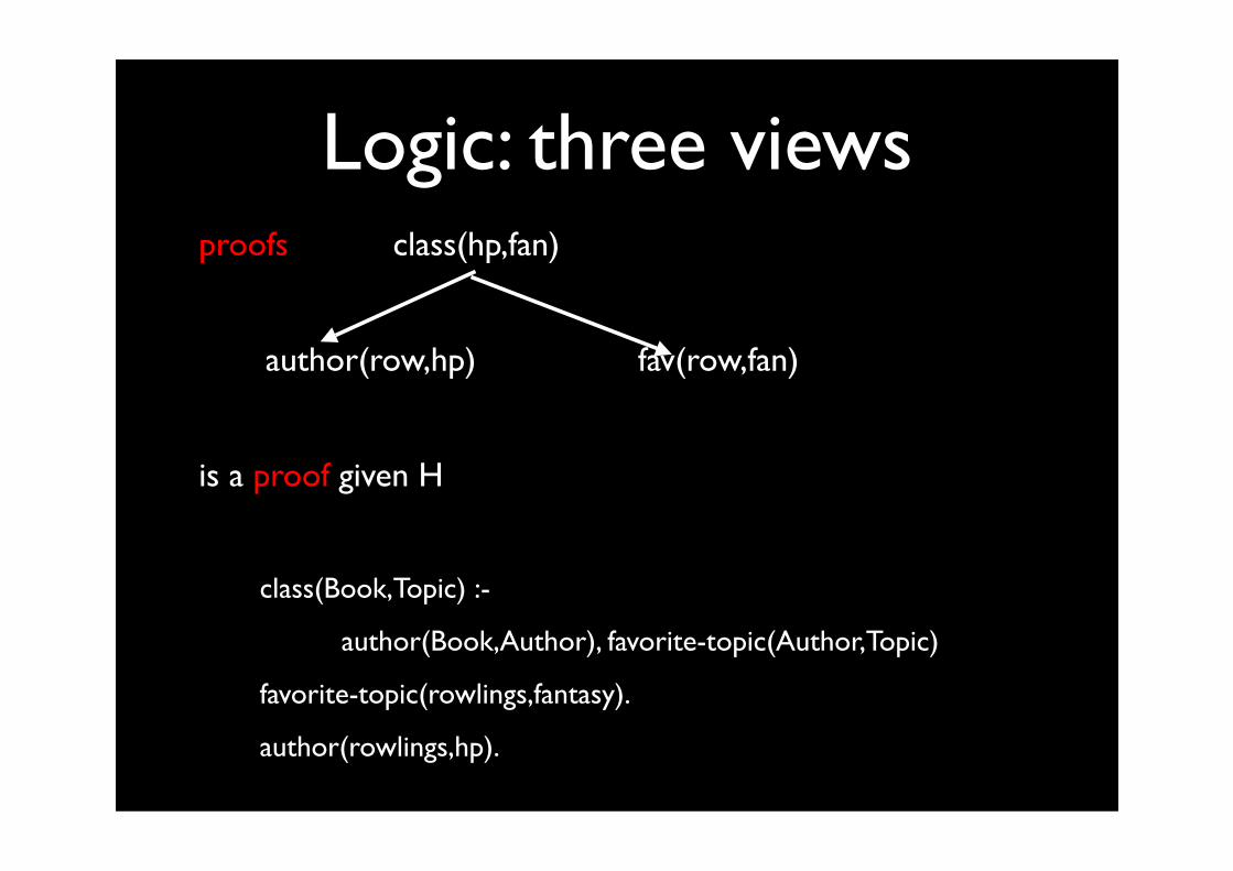
Logic: three viewsproofs class(hp,fan)
author(row,hp) fav(row,fan)
is a proof given H
class(Book,Topic) :-
author(Book,Author), favorite-topic(Author,Topic)
favorite-topic(rowlings,fantasy).
author(rowlings,hp).

BASICSlearning

Typical Machine Learning Problem
• Given
•a set of examples E
•various representational languages (and possibly background knowledge)
•a loss function
• Find
•A hypothesis h that minimizes the loss function w.r.t. the examples E
Different learning tasks
• classification
• regression
• clustering
• pattern mining
• ...

An LRL problem
class = positive IF there is a triangle inside a circle
A Bongard Problem

REPRESENTING the DATA

Represent the dataHierarchy
att
att
att
att att example
exampleexampleexampleexampleexampleexampleexampleexample
single-table single-tuple
attribute-value
att
att
att
att
att exampl
eexampl
e
example
single-table multiple-tuplemulti-instance
att
att
att
att
att
att
att
example
example
example
example
example
example
example
exampexa
att
att
att
att
att
att
att
examp
examp
exam
exam
exa
exa
exexe
multi-table multiple-tuple
relational
att
att
att
att
att
att
att
examp
examp
exam
exam
exa
exa
exexe
att
att
att
att
att
att
att
examp
examp
exam
exam
exa
exa
exexe
2 relationsedge / vertex
graphs & networks

Attribute-Valueatt
att
att
att att example
exampleexampleexampleexampleexampleexampleexampleexample
single-table single-tuple
attribute-value
Traditional Setting in Machine Learning(cf. standard tools like Weka)

Multi-Instanceatt
att
att
att
att exampl
eexampl
e
example
single-table multiple-tuplemulti-instance
[Dietterich et al. AIJ 96]
An example is positive if there exists a tuple in the example that satisfies particular properties
Boundary case between relational and propositional learning.
A lot of interest in past 10 years
Applications: vision, chemo-informatics, ...

Encoding Graphs

Encoding Graphs
atom(1,cl).atom(2,c).atom(3,c).atom(4,c).atom(5,c).atom(6,c).atom(7,c).atom(8,o)....
bond(3,4,s).bond(1,2,s).bond(2,3,d)....
12
34
76
5
9
8
14 10
1312
11
1615
17

Encoding Graphsatom(1,cl,21,0.297)
atom(2,c,21, 0187)
atom(3,c,21,-0.143)
atom(4,c,21,-0.143)
atom(5,c,21,-0.143)
atom(6,c,21,-0.143)
atom(7,c,21,-0.143)
atom(8,o,52,0.98)
...
bond(3,4,s).
bond(1,2,s).
bond(2,3,d).
...
12
34
76
5
9
8
14 10
1312
11
1615
17
Note: add identifier for molecule
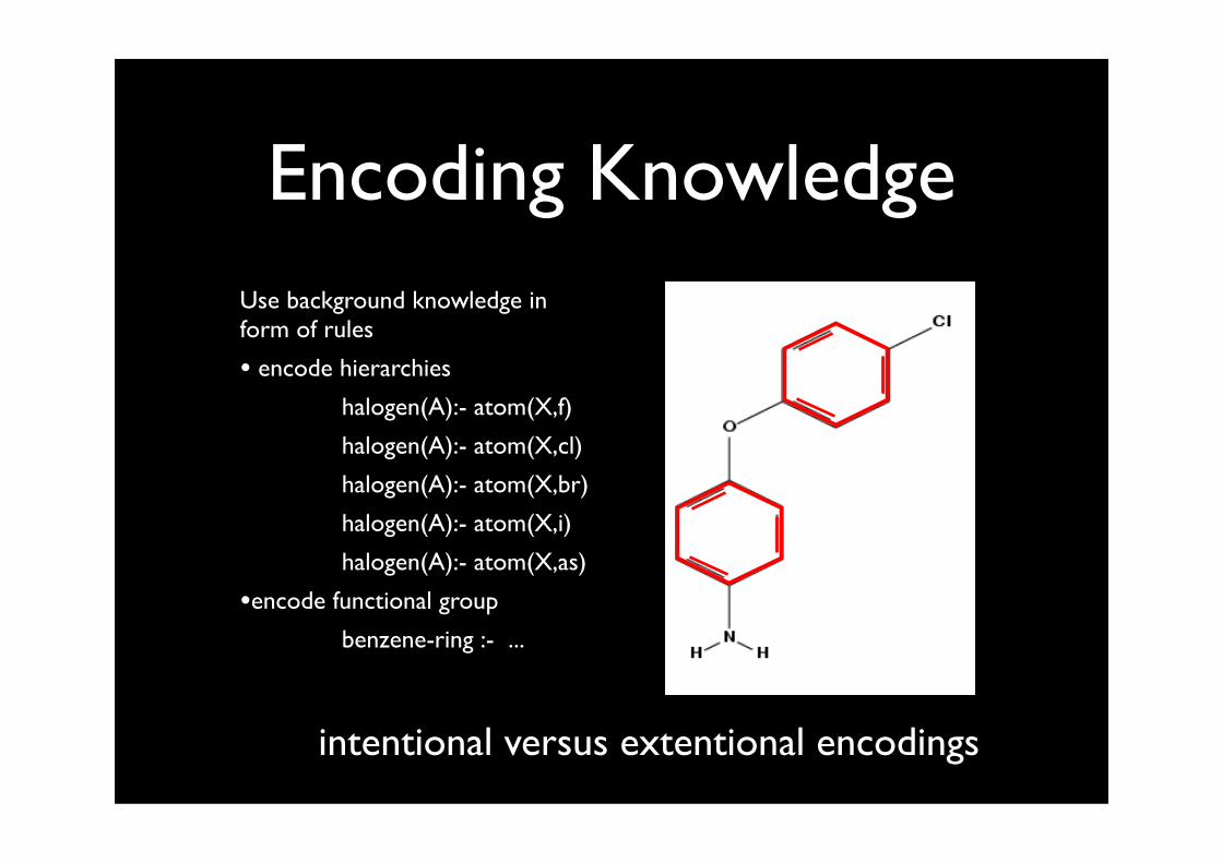
Encoding KnowledgeUse background knowledge in form of rules
• encode hierarchies
halogen(A):- atom(X,f)
halogen(A):- atom(X,cl)
halogen(A):- atom(X,br)
halogen(A):- atom(X,i)
halogen(A):- atom(X,as)
•encode functional group
benzene-ring :- ...
intentional versus extentional encodings

Relational Representation
12
34
76
5
9
8
14 10
1312
11
1615
17
att
att
att
att
att
att
att
example
example
example
example
example
example
example
exampexa
att
att
att
att
att
att
att
examp
examp
exam
exam
exa
exa
exexe
multi-table multiple-tuple
relational
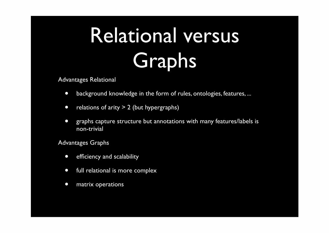
Relational versus Graphs
Advantages Relational
• background knowledge in the form of rules, ontologies, features, ...
• relations of arity > 2 (but hypergraphs)
• graphs capture structure but annotations with many features/labels is non-trivial
Advantages Graphs
• efficiency and scalability
• full relational is more complex
• matrix operations

The Hierarchy att
att
att
att att example
exampleexampleexampleexampleexampleexampleexampleexample
single-table single-tuple
attribute-value
att
att
att
att
att exampl
eexampl
e
example
single-table multiple-tuplemulti-instance
att
att
att
att
att
att
att
example
example
example
example
example
example
example
exampexa
att
att
att
att
att
att
att
examp
examp
exam
exam
exa
exa
exexe
multi-table multiple-tuple
relational
att
att
att
att
att
att
att
examp
examp
exam
exam
exa
exa
exexe
att
att
att
att
att
att
att
examp
examp
exam
exam
exa
exa
exexe
2 relationsedge / vertex
graphs & networks
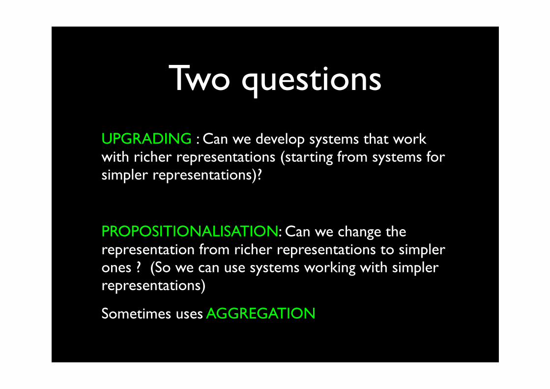
Two questions
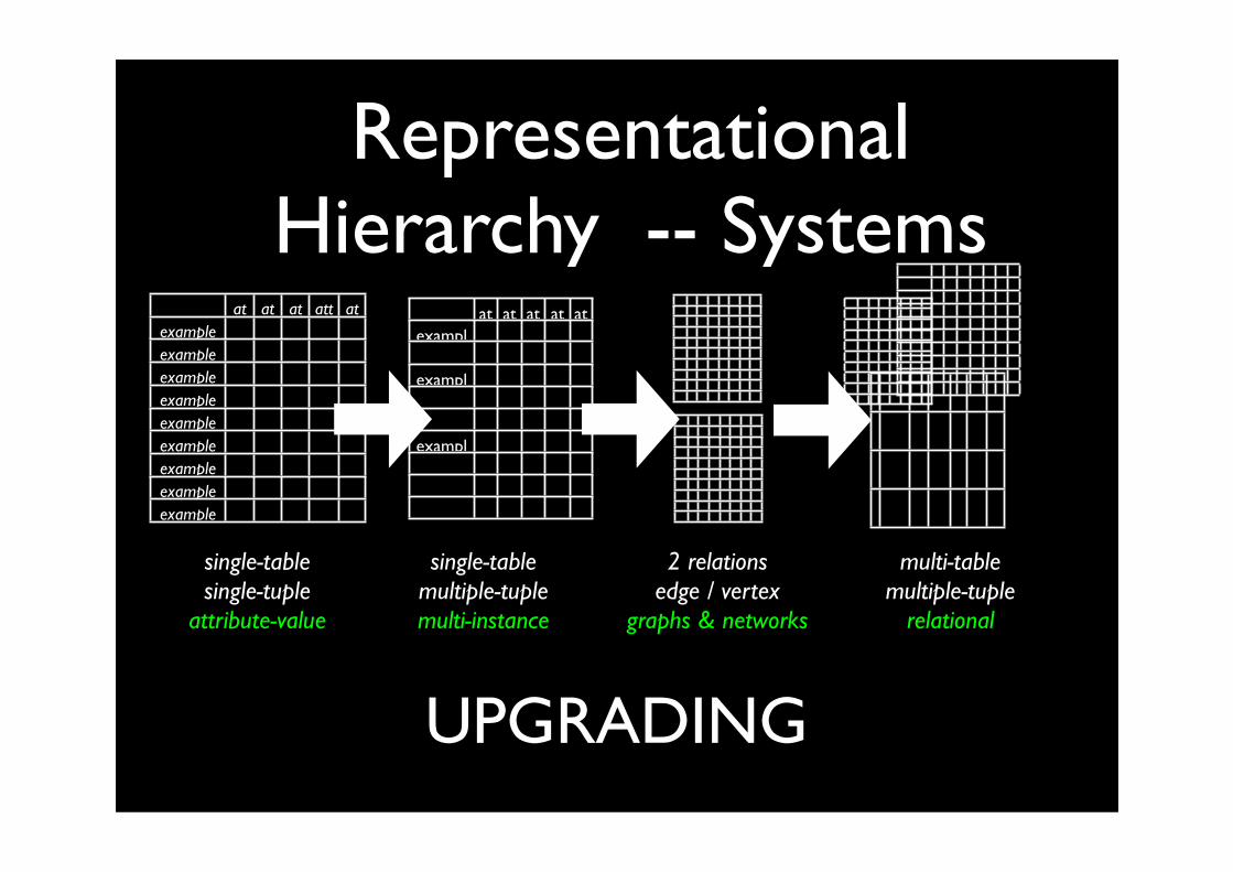
UPGRADING : Can we develop systems that work with richer representations (starting from systems for simpler representations)?
PROPOSITIONALISATION: Can we change the representation from richer representations to simpler ones ? (So we can use systems working with simpler representations)
Sometimes uses AGGREGATION
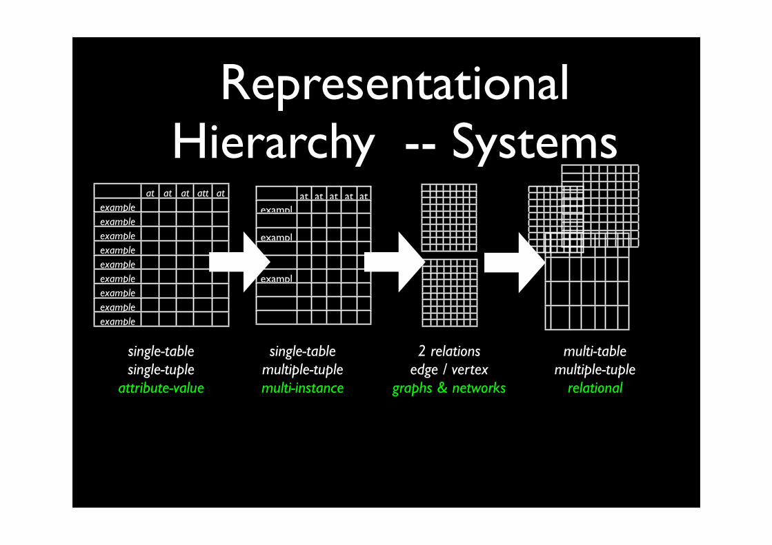
Representational Hierarchy -- Systems
att
att
att
att att example
exampleexampleexampleexampleexampleexampleexampleexample
single-table single-tuple
attribute-value
att
att
att
att
att exampl
eexampl
e
example
single-table multiple-tuplemulti-instance
att
att
att
att
att
att
att
example
example
example
example
example
example
example
exampexa
att
att
att
att
att
att
att
examp
examp
exam
exam
exa
exa
exexe
multi-table multiple-tuple
relational
att
att
att
att
att
att
att
examp
examp
exam
exam
exa
exa
exexe
att
att
att
att
att
att
att
examp
examp
exam
exam
exa
exa
exexe
2 relationsedge / vertex
graphs & networks

The Upgrading Methodology
Start from existing system for simpler representation
Extend it for use with richer representation (while trying to keep the original system as a special case)
Illustrations follow.

Learning Tasks
• rule-learning & decision trees [Quinlan 90], [Blockeel 96]
• frequent and local pattern mining [Dehaspe 98]
• distance-based learning (clustering & instance-based learning) [Horvath, 01], [Ramon 00]
• probabilistic modeling (cf. statistical relational learning)
• reinforcement learning [Dzeroski et al. 01]
• kernel and support vector methods
Logical and relational representations can (and have been) used for all learning tasks and techniques

Propositionalization
att
att
att
att att example
exampleexampleexampleexampleexampleexampleexampleexample
single-table single-tuple
attribute-value
att
att
att
att
att exampl
eexampl
e
example
single-table multiple-tuplemulti-instance
att
att
att
att
att
att
att
example
example
example
example
example
example
example
exampexa
att
att
att
att
att
att
att
examp
examp
exam
exam
exa
exa
exexe
multi-table multiple-tuple
relational
att
att
att
att
att
att
att
examp
examp
exam
exam
exa
exa
exexe
att
att
att
att
att
att
att
examp
examp
exam
exam
exa
exa
exexe
2 relationsedge / vertex
graphs & networks
Downgrading the data ?

Propositionalization
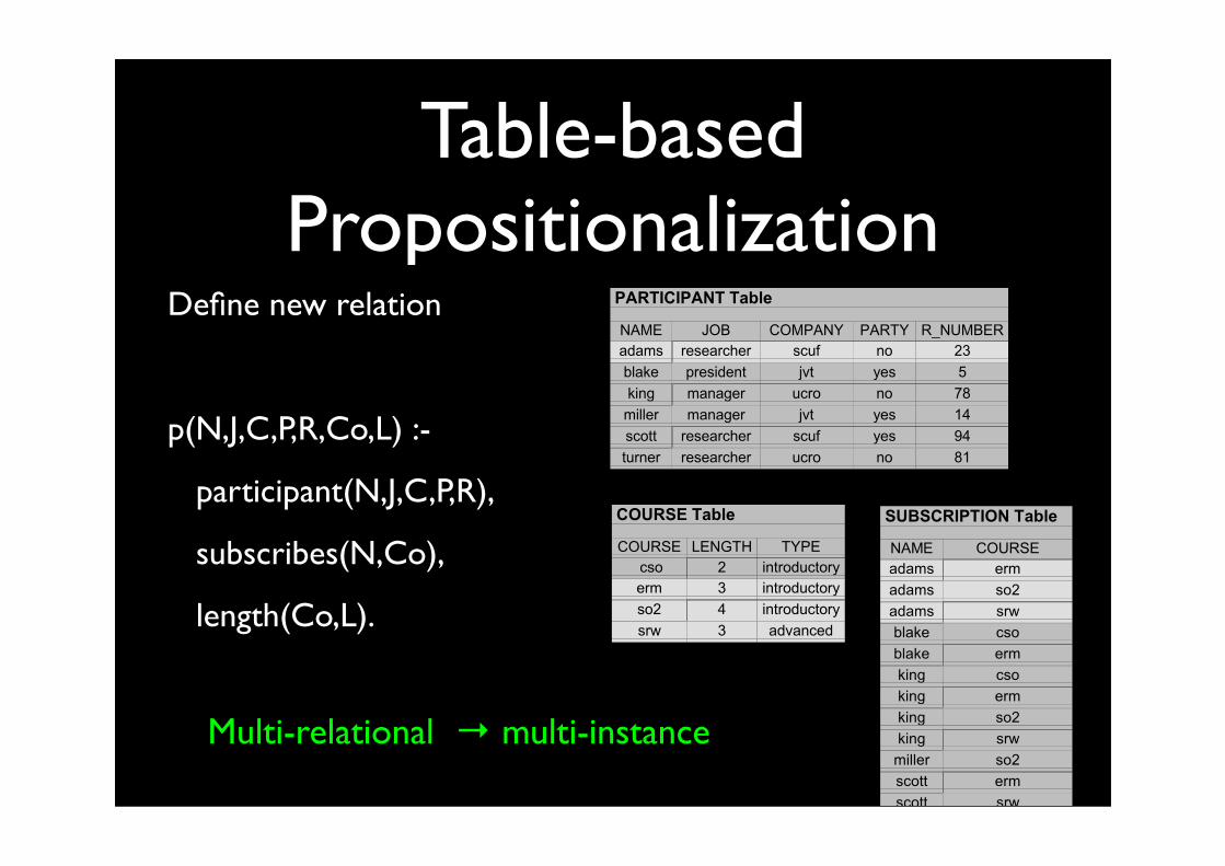
Table-based Propositionalization
Define new relation
p(N,J,C,P,R,Co,L) :-
participant(N,J,C,P,R),
subscribes(N,Co),
length(Co,L).
Multi-relational → multi-instance

Table-based Propositionalization
Examples are subscriptions
instead of participants
s(N,J,C,P,R,Co,L) :-
participant(N,J,C,P,R),
subscribes(N,Co),
length(Co,L).
Under certain conditions Multi-relational --> attribute value
directly feed into standard ML systems

Table-based Propositionalization
1 tuple for participant/5
gives n tuples for p/7
p(N,J,C,P,R,Co,L) :-
participant(N,J,C,P,R),
subscribes(N,Co),
length(Co,L).
Multi-relational → multi-instanceunder certain conditions → atttribute-value

Query-basedPropositionalization
Compute a set of relevant features or queries.
Typically, (variant of) local pattern mining; also heuristic approaches
E.g. find all frequent or correlated subgraphs.
Use each feature as boolean attribute.
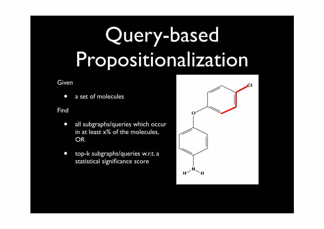
Query-basedPropositionalization
Given
• a set of molecules
Find
• all subgraphs/queries which occur in at least x% of the molecules, OR
• top-k subgraphs/queries w.r.t. a statistical significance score
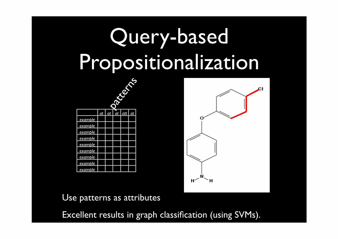
Query-basedPropositionalization
att
att
att
att att example
exampleexampleexampleexampleexampleexampleexampleexample
patte
rns
Use patterns as attributes
Excellent results in graph classification (using SVMs).
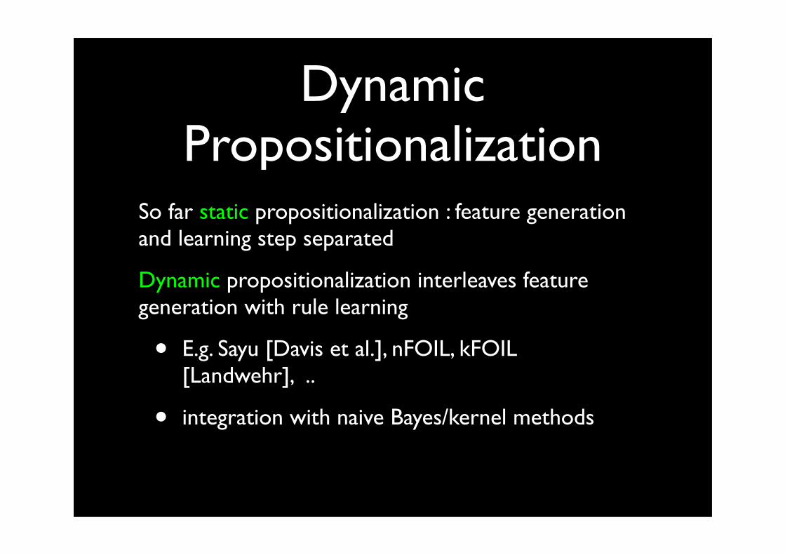
Dynamic Propositionalization
So far static propositionalization : feature generation and learning step separated
Dynamic propositionalization interleaves feature generation with rule learning
• E.g. Sayu [Davis et al.], nFOIL, kFOIL [Landwehr], ..
• integration with naive Bayes/kernel methods
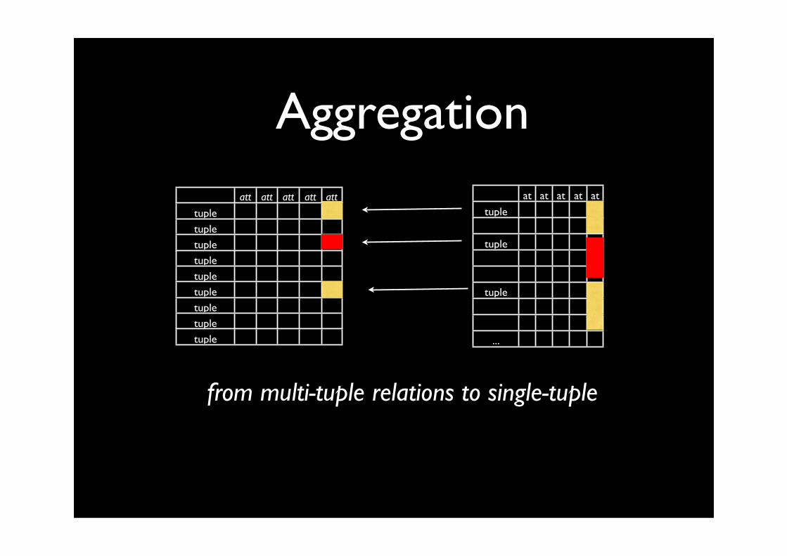
Aggregationatt att att att att
tupletupletupletupletupletupletupletupletuple
att
att
att
att
att tuple
tuple
tuple
...
from multi-tuple relations to single-tuple

Introduce new attribute
For instance :
• number of courses followed
multi-instance/tuple → attribute-value
Aggregation
adams, 3

Propositionalization and Aggregation
Often useful to reduce more expressive representation to simpler one but almost always results in information loss or combinatorial explosion
Shifts the problem
• how to find the right features / attributes ?
One example
• features = paths in a graph (for instance)
• which ones to select ?
still requires “relational” methods

The LOGIC of LEARNING Coverage and Generality

Typical Machine Learning ProblemGiven
•a set of examples E
•a background theory B
•a logic language Le to represent examples
•a logic language Lh to represent hypotheses
•a covers relation on Le x Lh
•a loss function
Find
•A hypothesis h in Lh that minimizes the loss function w.r.t. the examples E taking B into account

o
Covers Relation

Covers Relation
o
12
34
76
5
9
8
14 10
1312
11
1615
17
A BC
D
EF
G
Subgraph Isomorphism(bijection)
or Homomorphism
(injection)

Coverage
OI-subsumption(bijection)
or theta-subsumption
(injection)
atom(1,cl).atom(2,c).atom(3,c).atom(4,c).atom(5,c).atom(6,c).atom(7,c).atom(8,o)....
bond(3,4,s).bond(1,2,s).bond(2,3,d)....
positive :- atom(A,c), atom(B,c),
bond(A,B,s),....
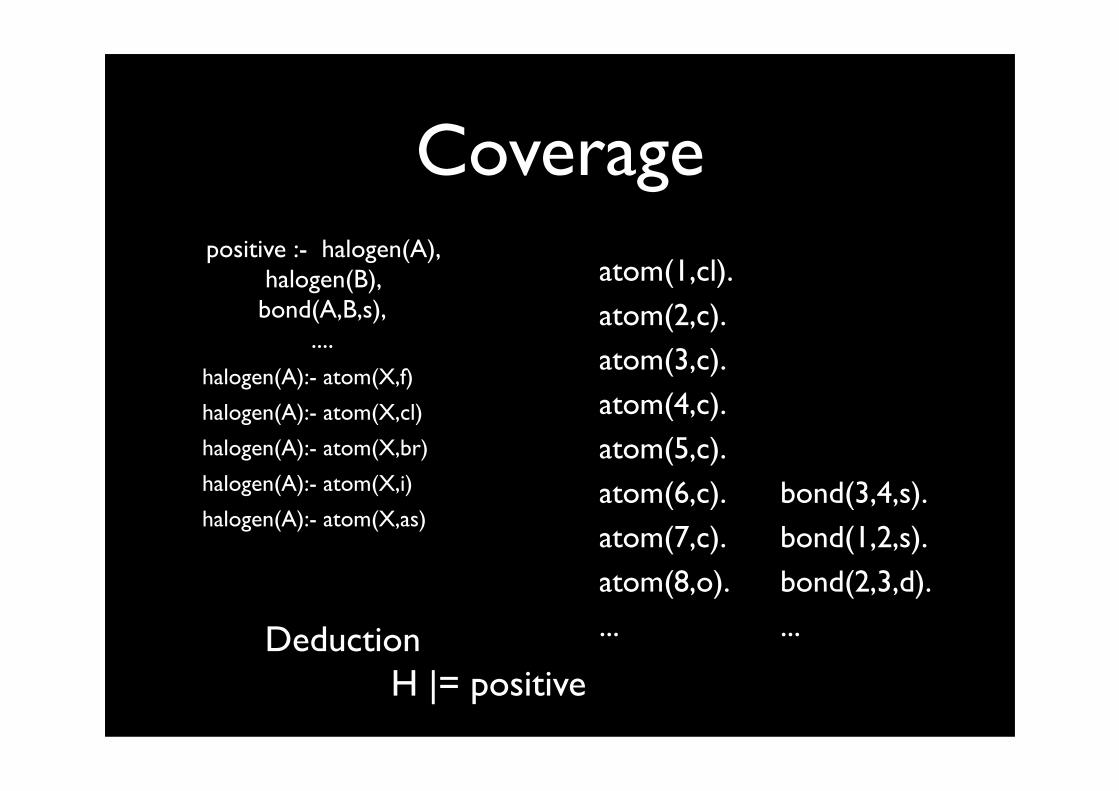
Coverage
Deduction
atom(1,cl).atom(2,c).atom(3,c).atom(4,c).atom(5,c).atom(6,c).atom(7,c).atom(8,o)....
bond(3,4,s).bond(1,2,s).bond(2,3,d)....
positive :- halogen(A), halogen(B), bond(A,B,s),
....halogen(A):- atom(X,f)
halogen(A):- atom(X,cl)
halogen(A):- atom(X,br)
halogen(A):- atom(X,i)
halogen(A):- atom(X,as)
H |= positive

Logic: three viewsentailment/logical consequence
H |= class(harrypotter,fantasy)
class(harrypotter,fantasy) follows from H
models {class(hp,fan), author(row,hp), fav(row,fan)}
is a model for H
is a possible world given H
proofs class(hp,fan)
author(row,hp) fav(row,fan)

Three possible SETTINGS
Learning from entailment (FOIL)
• covers(H,e) iff H |= e
Learning from interpretations
• covers(H,e) iff e is a model for H
Learning from proofs or traces.
• covers(H,e) iff e is proof given H
The setting can matter a lotA Knowledge Representation Issue
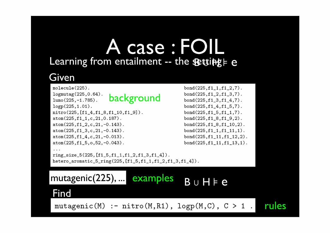
A case : FOILLearning from entailment -- the setting
Given
mutagenic(225), ...
Find
background
examples
rules
B ∪ H ⊧ e
B ∪ H ⊧ e

Learning from entailment
Learning from entailment -- the setting
Given
mutagenic(225), ...
Find
background
examples
rules
B ∪ H ⊧ e
covers(H,e) iff H |= e or B ∪ H ⊧ e
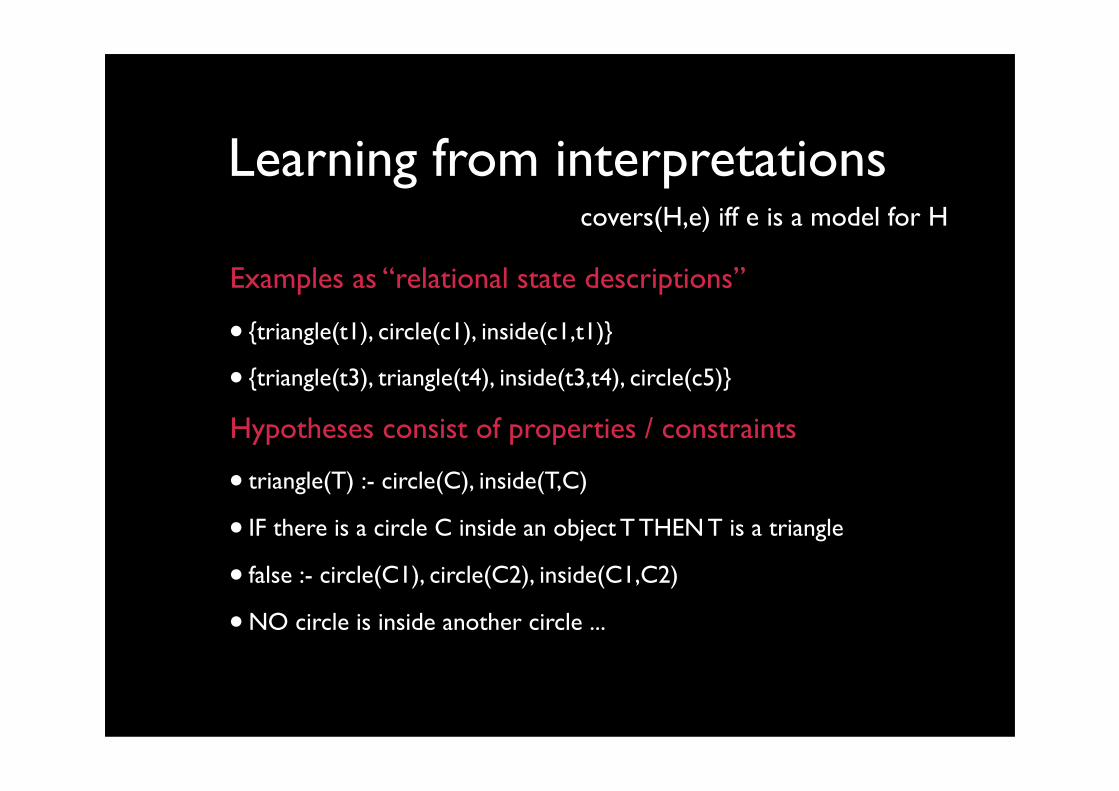
Learning from interpretations
Examples as “relational state descriptions”
• {triangle(t1), circle(c1), inside(c1,t1)}
• {triangle(t3), triangle(t4), inside(t3,t4), circle(c5)}
Hypotheses consist of properties / constraints
• triangle(T) :- circle(C), inside(T,C)
• IF there is a circle C inside an object T THEN T is a triangle
• false :- circle(C1), circle(C2), inside(C1,C2)
• NO circle is inside another circle ...
covers(H,e) iff e is a model for H
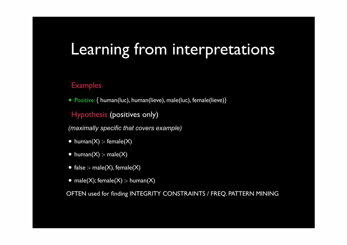
Learning from interpretations
Examples
• Positive: { human(luc), human(lieve), male(luc), female(lieve)}
Hypothesis (positives only)
(maximally specific that covers example)
• human(X) :- female(X)
• human(X) :- male(X)
• false :- male(X), female(X)
• male(X); female(X) :- human(X)
OFTEN used for finding INTEGRITY CONSTRAINTS / FREQ. PATTERN MINING

Learning from ProofsExamples
Hypothesis
Used in Treebank Grammar Learning & Program Synthesis
covers(H,e) iff e is proof given H
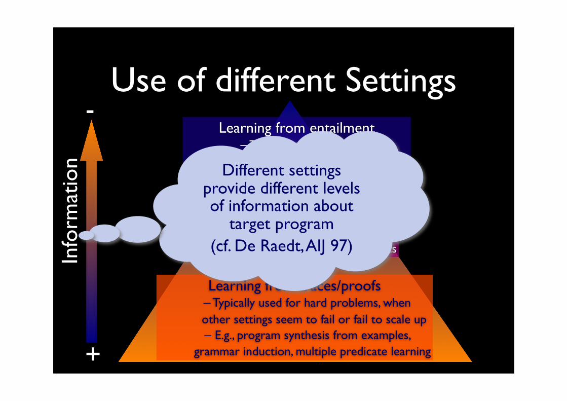
Use of different Settings
Learning from interpretations– Typically used for description
– E.g., inducing integrity constraints
Learning from entailment– The most popular setting
– Typically used for prediction– E.g., predicting activity of compounds
Learning from traces/proofs– Typically used for hard problems, when
other settings seem to fail or fail to scale up– E.g., program synthesis from examples,
grammar induction, multiple predicate learning
-
+
Info
rmat
ion Different settings
provide different levels of information about
target program (cf. De Raedt, AIJ 97)

Generality Relation
An essential component of symbolic learning / mining systems.
Clauses
positive :- outlook(sunny), temperature(high)
is more general than
positive :- outlook(sunny), temperature(high), wind(strong)
all examples covered by 2nd clause also covered by 1st
used to structure the search space in mining and learning systems

Using Generality
To define the search space that is traversed.
Cf. frequent item-set mining, concept-learning.

Different types of search strategy:
all solutions (freq. item-sets), top-k solutions (branch and bound algo.), heuristic (concept-learning)
Generality
lexicographic order/canonical form
just add an item

Generality RelationAn essential component of Symbolic Learning systems
G is more general than S if all examples covered by S are also covered by G
Using graphs
• subgraph isomorphism or homomorphism
In logic
• theta or OI subsumption, in general G ⊧ S

Generality Relation
positive :- atom(X,c) ⊧ positive :- atom(X,c), atom(Y,o)
but also
positive :- halogen(X)
halogen(X) :- atom(X,c) ⊧ positive :- atom(X,c)

G ⊧ S
S follows deductively from G
G follows inductively from S
therefore induction is the inverse of deduction
this is an operational point of view because there are many deductive operators ⊦ that implement ⊧
take any deductive operator and invert it and one obtains an inductive operator

Various frameworks for generality
Depending on the form of G and S
single clause
clausal theory
Relative to a background theory B U G ⊧ S
Depending on the choice of ⊦ to invert
subsumption (most popular)

Subsumption in 3 Steps
Subsumption ~ generalization of graph morphisms
1. propositional
2. atoms
3. clauses (rules)

Propositional Logic
{f,¬b,¬n} = f IF b and n = f :- b, nG ⊧ S if and only if G ⊆ S
just like item-sets

Logical Atoms
Does g=participant(adams, X, kul) match
s=participant(adams,researcher, kul) ?
Yes, because there is a substitution θ={X/researcher} such that gθ=s
more complicated, account for variable unification

Subsumption in Clauses
Combine propositional and atomic subsumption.
G subsumes S if and only if there is a substitution θ such that Gθ⊆S.
Graph - homomorphism as special case

Subsumption Relation
o
12
34
76
5
9
8
14 10
1312
11
1615
17
A BC
D
EF
G
Subgraph Isomorphism(bijection)
or Homomorphism
(injection)θ={G/8,A/5,B/4,C/3,D/2,E/7,F/6}

SubsumptionWell-understood and studied, but complicated.
Testing subsumption (and subgraph-ismorphism) is NP-complete
Infinite chains (up and downwards) exist
Syntactic variants exist when working with homomorphism (but not for isomorphism).
Computation of lub (lgg) and glb
Sound but incomplete, i.e. when G θ-subsumes S implies that G |= S, but not vice versa, e.g.
• p(f(X)) :- p(X) and p(f(f(Y))) :- p(Y).

Subsumption
OI-subsumption(bijection)
or theta-subsumption
(injection)
atom(1,cl).atom(2,c).atom(3,c).atom(4,c).atom(5,c).atom(6,c).atom(7,c).atom(8,o)....
bond(3,4,s).bond(1,2,s).bond(2,3,d)....
positive :- atom(A,c), atom(B,c),
bond(A,B,s),....
θ={G/8,A/5,B/4,C/3,D/2,E/7,F/6}

Theta-subsumption lattice
subgraph homomorphismnot a lattice when working with isomorphism
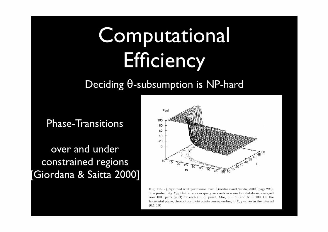
Computational Efficiency
Deciding θ-subsumption is NP-hard
Phase-Transitions
over and under constrained regions
[Giordana & Saitta 2000]

Computational Efficiency
Deciding θ-subsumption is NP-hard

Generality relations and refinement operators are well-understood; they apply to simpler structures such as graphs (canonical form -- lexicographic orders)
G ⊧ S

Refinement
Graphs :
Adding edges
Relational learning
Adding literals
bond(A,B,s),
bond(B,C,d), ...
Applying a substitution
{A = B} or {C = cl}

Refinement operators
Apply a substitution
or add a literal
Various properties of refinement operators studiede.g. Nienhuys-Cheng & De Wolf

Alternative frameworksInverse implication (addressing incompleteness θ-subsumption)
Inverting the resolution principle (Muggleton and Buntine, 88)
grandparent(X,Y) :- father(X,Z), parent(Z,Y)father(X,Y) :- male(X), parent(X,Y)
grandparent(X,Y) :- male(X), parent(X,Z), parent(Z,Y)
parent(jef,an)
male(jef)
grandparent(jef,Y) :- parent(jef,Z), parent(Z,Y)
grandparent(jef,Y) :- parent(an,Y)parent(an,paul)
grandparent(jef,paul)
resolution

Operators
G and S are sets of clauses and
Absorption :
Identification

Operators
Intra-construction
Inter-construction

Predicate Invention
Applying Intra-construction
Yields (where newp is a new predicate)

Inverse EntailmentB U h |= e iff B U ¬e |= ¬h
find all atoms entailed by BU¬ e
call this ¬h and negate again to give maximally specific h called bottom clause
B = { mammal(X) :- dog(X); mammal(X) :- cat(X); cat(saar) }e = nice(saar)
let bias assume arguments in examples must be mentioned in entailed facts !
B U ¬ e |= mammal(saar), cat(saar), ¬ nice(saar)gives h = nice(saar) :- mammal(saar), cat(saar)
Used in Muggleton’s Progol, Srinivasan’s Aleph

Bounded Search in Progol
nice(saar) :- mammal(saar), cat(saar)
dog does not appear in search !
nice(X)
nice(saar) nice(X) :- mammal(X)
nice(X) :- cat(X) …..

Generality relations and refinement operators are well-understood; they apply to simpler structures such as graphs (canonical form -- lexicographic orders)
G ⊧ S

SYSTEMS & METHODOLOGY
Representational Hierarchy -- Systems
att
att
att
att att example
exampleexampleexampleexampleexampleexampleexampleexample
single-table single-tuple
attribute-value
att
att
att
att
att exampl
eexampl
e
example
single-table multiple-tuplemulti-instance
att
att
att
att
att
att
att
example
example
example
example
example
example
example
exampexa
att
att
att
att
att
att
att
examp
examp
exam
exam
exa
exa
exexe
multi-table multiple-tuple
relational
att
att
att
att
att
att
att
examp
examp
exam
exam
exa
exa
exexe
att
att
att
att
att
att
att
examp
examp
exam
exam
exa
exa
exexe
2 relationsedge / vertex
graphs & networks
UPGRADING

Two messages
LRL applies essentially to any machine learning and data mining task, not just concept-learning
• distance based learning, clustering, descriptive learning, reinforcement learning, bayesian approaches
there is a recipe that is being used to derive new LRL algorithms on the basis of propositional ones
• not the only way to LRL

Learning Tasks
• rule-learning & decision trees [Quinlan 90], [Blockeel 96]
• frequent and local pattern mining [Dehaspe 98]
• distance-based learning (clustering & instance-based learning) [Horvath, 01], [Ramon 00]
• probabilistic modeling (cf. statistical relational learning)
• reinforcement learning [Dzeroski et al. 01]
• kernel and support vector methods
Logical and relational representations can (and have been) used for all learning tasks and techniques

The RECIPE
Start from well-known propositional learning system
Modify representation and operators
• e.g. generalization/specialization operator, similarity measure, …
• often use theta-subsumption as framework for generality
Build new system, retain as much as possible from propositional one

LRL Systems and techniques
FOIL ~ CN2 – Rule Learning (Quinlan MLJ 90)
Tilde ~ C4.5 – Decision Tree Learning (Blockeel & DR AIJ 98)
Warmr ~ Apriori – Association rule learning (Dehaspe 98)
Progol ~~ AQ – Rule learning (Muggleton NGC 95)
Graph miners ...
Distance based learning
Reinforcement learning

A case : FOILLearning from entailment -- the setting
Given
mutagenic(225), ...
Find
background
examples
rules
B ∪ H ⊧ e
B ∪ H ⊧ e

Searching for a rule
:- true
Coverage = 0.65
Coverage = 0.7
Coverage = 0.6
:- atom(X,A,c)
:- atom(X,A,n)
:- atom(X,A,f)
Coverage = 0.6
Coverage = 0.75
:- atom(X,A,n),bond(A,B)
:- atom(X,A,n),charge(A,0.82)
Greedy separate-and-conquer for rule setGreedy general-to-specific search for single rule

Searching for a rule
:- true
Coverage = 0.65
Coverage = 0.7
Coverage = 0.6
:- atom(X,A,c)
:- atom(X,A,n)
:- atom(X,A,f)
Coverage = 0.6
Coverage = 0.75
:- atom(X,A,n),bond(A,B)
:- atom(X,A,n),charge(A,0.82)
mutagenic(X) :- atom(X,A,n),charge(A,0.82)
Greedy separate-and-conquer for rule setGreedy general-to-specific search for single rule
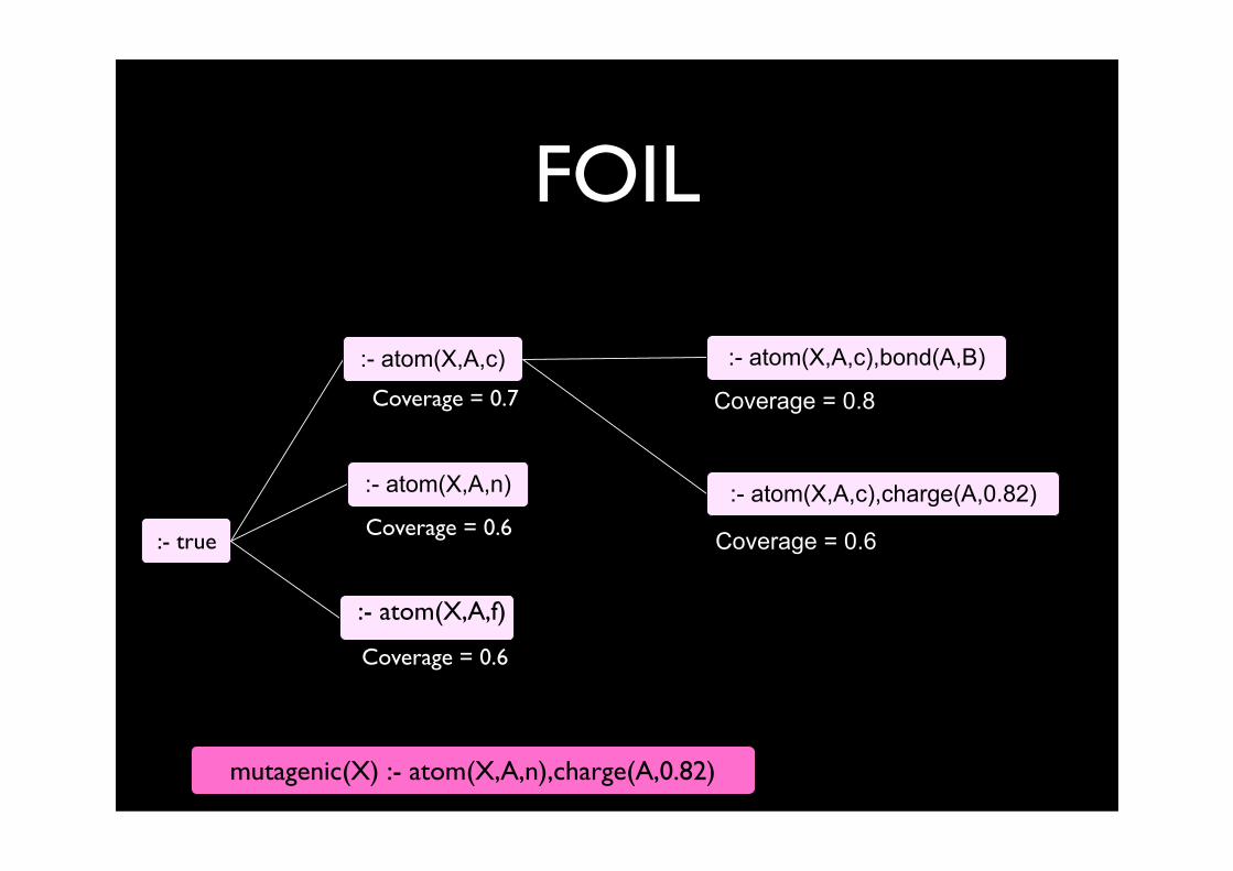
FOIL
mutagenic(X) :- atom(X,A,n),charge(A,0.82)
:- true
Coverage = 0.7
Coverage = 0.6
Coverage = 0.6
:- atom(X,A,c)
:- atom(X,A,n)
:- atom(X,A,f)
Coverage = 0.8
Coverage = 0.6
:- atom(X,A,c),bond(A,B)
:- atom(X,A,c),charge(A,0.82)

FOIL
mutagenic(X) :- atom(X,A,n),charge(A,0.82)
:- true
Coverage = 0.7
Coverage = 0.6
Coverage = 0.6
:- atom(X,A,c)
:- atom(X,A,n)
:- atom(X,A,f)
Coverage = 0.8
Coverage = 0.6
:- atom(X,A,c),bond(A,B)
:- atom(X,A,c),charge(A,0.82)
mutagenic(X) :- atom(X,A,c),bond(A,B)

mutagenic(X) :- atom(X,A,n),charge(A,0.82)
mutagenic(X) :- atom(X,A,c),bond(A,B)
mutagenic(X) :- atom(X,A,c),charge(A,0.45)

TildeLogical Decision Trees (Blockeel & De Raedt AIJ 98)

A logical decision tree

WARMR

What to count ? Keys.
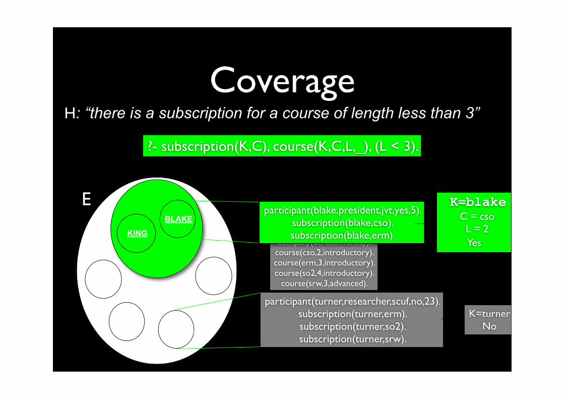
Coverage
company(jvt,commercial).company(scuf,university).company(ucro,university).
course(cso,2,introductory).course(erm,3,introductory).course(so2,4,introductory).
course(srw,3,advanced).
H: “there is a subscription for a course of length less than 3”
participant(blake,president,jvt,yes,5).subscription(blake,cso).subscription(blake,erm).
?- subscription(K,C), course(K,C,L,_), (L < 3).
participant(turner,researcher,scuf,no,23).subscription(turner,erm).subscription(turner,so2).subscription(turner,srw).
K=blake C = cso L = 2
Yes
K=turnerNo
EBLAKE
KING
TURNERSCOTT
MILLER ADAMS

Descriptive Data Mining
Selected,Preprocessed,
and Transformed Data
multi-relational database
association rules over multiple relations
“IF participant follows an advanced course THEN she skips the welcome party”
support: 20 %confidence: 75 %
“IF ?- participant(P,C,PA,X), course(P,Y,advanced)
THEN ?-PA = no.
support: 20 %confidence: 75 %

Warmr
First order association rule :
• IF Query1 THEN Query2 Shorthand for
• IF Query1 THEN Query1 and Query2 to obtain variable bindings
IF ?- participant(P,C,PA,X), course(P,Y,advanced) THEN PA=no
IF ?- participant(P,C,PA,X), course(P,Y,advanced) succeeds for P
THEN ?- participant(P,C,PA,X), course(P,Y,advanced), PA=no succeeds for P
Counting : number of ‘keys’ for which queries succeed

Warmr ~ Apriori
Works as Apriori :
• keeping track of frequent and infrequent queries
• order queries by theta-subsumption
• using special mechanism (bias) to declare type of queries searched for
Generalizes many of the specific variants of Apriori : item-sets, episodes, hierarchies, intervals, ...

Upgrading
Key ideas / contributions FOIL + Tilde + Warmr
• determine the representation of examples and hypotheses
• select the right type of coverage and generality (subsumption)
• keep existing algorithm (CN2 or C4.5) but replace operators (often theta-subsumption)
• keep search strategy
• fast implementation

Distance Based Learning
De Raedt, Ramon 2009
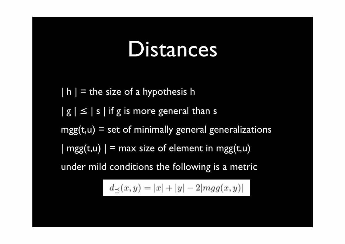
Distances
| h | = the size of a hypothesis h
| g | ≤ | s | if g is more general than s
mgg(t,u) = set of minimally general generalizations
| mgg(t,u) | = max size of element in mgg(t,u)
under mild conditions the following is a metric

Distances
Quite important in machine learning and data mining
• k-nearest neighbor algorithm
• agglomarative clustering
• ...
relation to kernel methods exists as well.

Learning TheoriesInstead of learning theories from scratch, revise
them
Example
T :grandparent(X,Y) :- parent(X,Z), parent(Z,Y)parent(jef,paul).
e: grandparent(jef,an) T’ :
assert(T, parent(paul,an)) assert(T, grandparent(jef,an))

ProblemsInterdependencies among clauses and examples; also
when learning recursive clauses or multiple predicates, key problem for program synthesis
Search at the level of SETS of clauses instead of at the level of single clauses
anc(X,Y) :- parent(X,Y).anc(X,Y) :- parent(X,Z), anc(Z,Y).
uncle(X,Y) :- brother(X,Z),parent(Z,Y).brother(X,Y) :- parent(W,Y),parent(W,X), male(X).
member(X,[X|Y])member(X,[U|Z]) :- member(X,Z)

The RECIPE
Relevant for ALL levels of the hierarchy
Still being applied across data mining,
• mining from graphs, trees, and sequences
Works in both directions
• upgrading and downgrading !!!
Mining from graphs or trees as downgraded
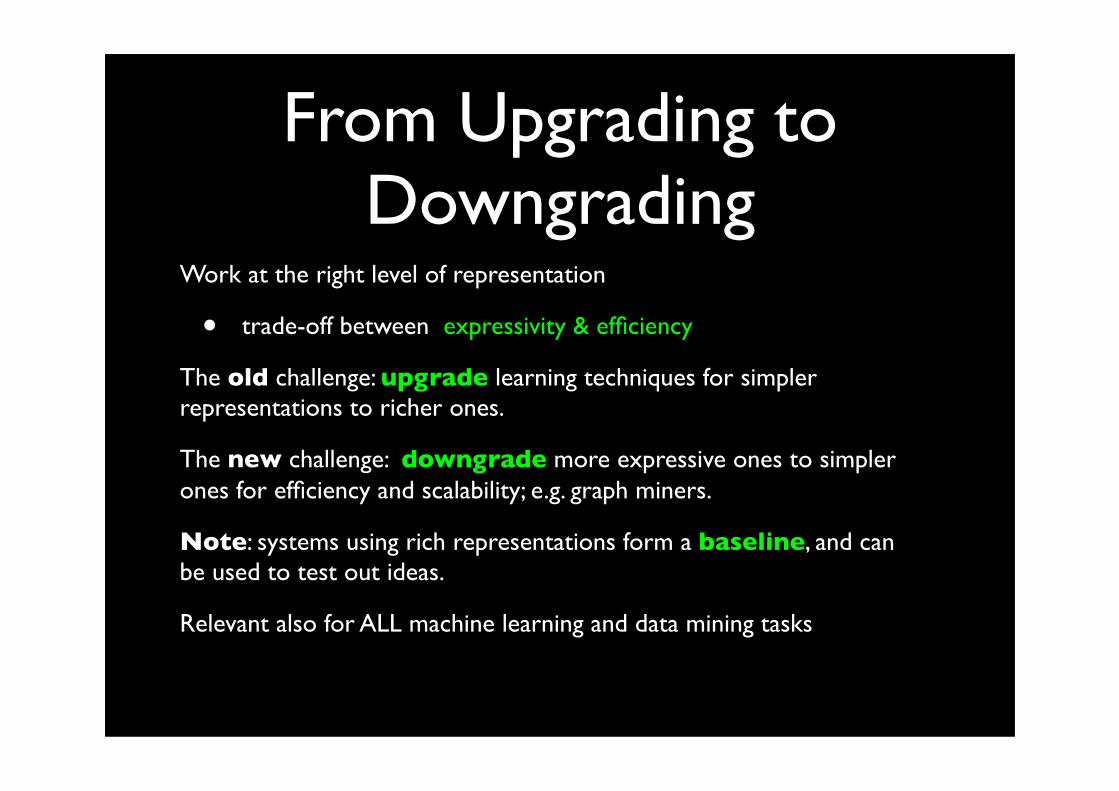
From Upgrading to Downgrading
Work at the right level of representation
• trade-off between expressivity & efficiency
The old challenge: upgrade learning techniques for simpler representations to richer ones.
The new challenge: downgrade more expressive ones to simpler ones for efficiency and scalability; e.g. graph miners.
Note: systems using rich representations form a baseline, and can be used to test out ideas.
Relevant also for ALL machine learning and data mining tasks

Learning Tasks
Logical and relational representations can (and have been) used for all learning tasks and techniques
• rule-learning & decision trees
• frequent and local pattern mining
• distance-based learning (clustering & instance-based learning)
• probabilistic modeling (cf. statistical relational learning)
• reinforcement learning
• kernel and support vector methods

LOGIC, RELATIONS and PROBABILITY
Joint work with Kristian Kersting et al.

Books
Also, survey paper De Raedt, Kersting, SIGKDD Explorations 03

Statistical Relational Learning
Logic and relations alone are often insufficient
• but can be combined with probabilistic reasoning and models
• use logic as a toolbox
Also known as Probabilistic Logic Learning, or Probabilistic Inductive Logic Programming

Some SRL formalisms
LPAD: Bruynooghe
Vennekens,VerbaetenMarkov Logic: Domingos,
RichardsonCLP(BN): Cussens,Page,
Qazi,Santos Costa
Present
PRMs: Friedman,Getoor,Koller,Pfeffer,Segal,Taskar
´03
SLPs: Cussens,Muggleton
´90 ´95 96
First KBMC approaches:
Breese,
Bacchus,Charniak,
Glesner,Goldman,
Koller,Poole, Wellmann
´00
BLPs: Kersting, De Raedt
RMMs: Anderson,Domingos,Weld
LOHMMs: De Raedt, Kersting,Raiko
Future
Prob. CLP: Eisele, Riezler
´02
PRISM: Kameya, Sato
´94
PLP: Haddawy, Ngo
´97´93
Prob. Horn Abduction: Poole
´99
1BC(2): Flach,Lachiche
Logical Bayesian Networks: Blockeel,Bruynooghe,
Fierens,Ramon,

PLL: What Changes ?
Clauses annotated with probability labels
• E.g. in Sato’s Prism, Eisele and Muggleton’s SLPs, Kersting and De Raedt’s BLPs, …
Prob. covers relation covers(e,H U B) = P(e | H,B)
• Probability distribution P over the different values e can take; so far only (true,false)
Knowledge representation issue
•Define probability distribution on examples / individuals
•What are these examples / individuals ? [cf. SETTINGS]

Probabilistic SRL Problem
Given
• a set of examples E
• a background theory B
• a language Le to represent examples
• a language Lh to represent hypotheses
• a probabilistic covers P relation on Le x Lh
Find
• hypothesis h* maximizing some score based on the probabilistic covers relation; often some kind of maximum likelihood

PLL: Three Issues
Defining Lh and P - KNOWLEDGE REPRESENTATION
•Clauses + Probability Labels
Learning Methods - MACHINE LEARNING
•Parameter Estimation
• Learning probability labels for fixed clauses
•Structure learning
• Learning both components

PLL: Three SettingsProbabilistic learning from interpretations
•Bayesian logic programs, Koller’s PRMs, Domingos’ MLNs, Vennekens’ LPADs/CP-logic
Probabilistic learning from entailment
•Cussens and Muggleton’s Stochastic Logic Programs, Sato’s Prism, Poole’s ICL, De Raedt et al.’s ProbLog
Probabilistic learning from proofs
•Learning the structure of SLPs; a tree-bank grammar based approach, Anderson et al.’s RMMs, Kersting et al.
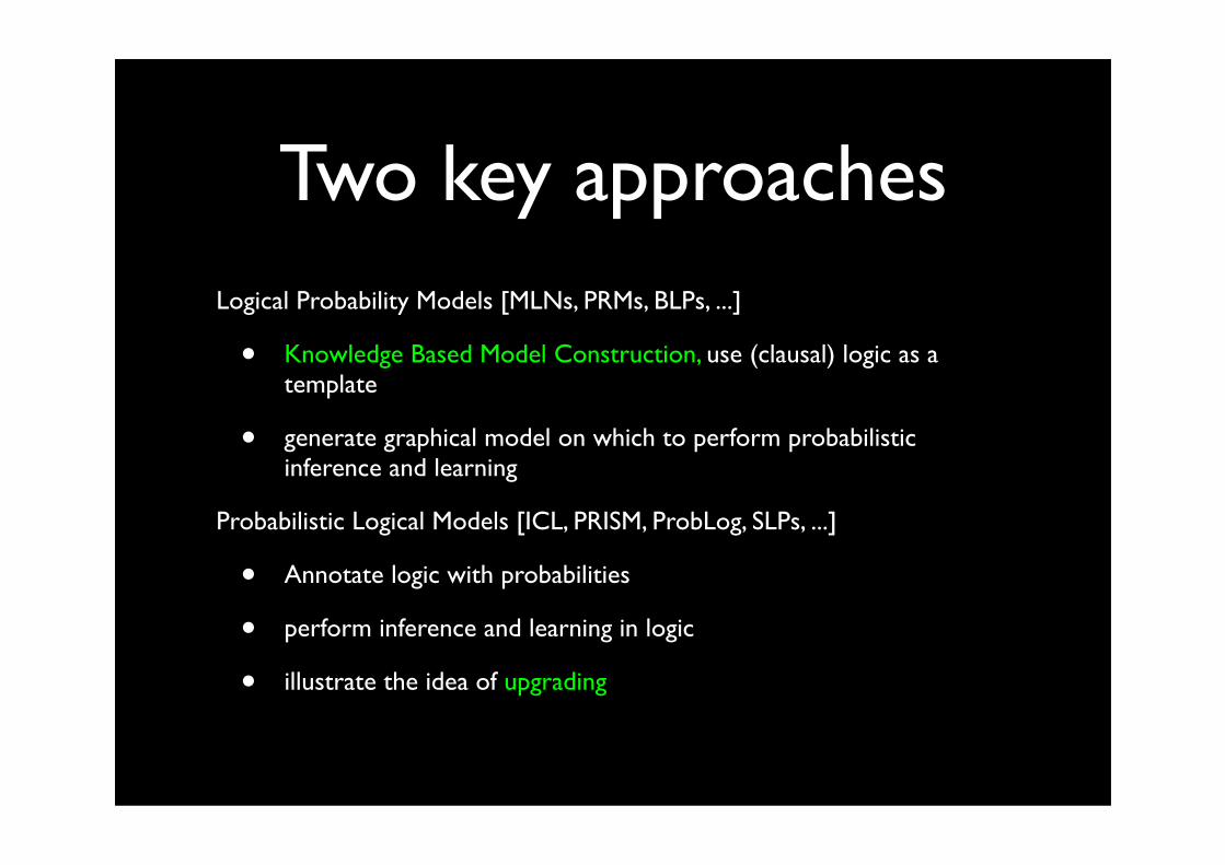
Two key approachesLogical Probability Models [MLNs, PRMs, BLPs, ...]
• Knowledge Based Model Construction, use (clausal) logic as a template
• generate graphical model on which to perform probabilistic inference and learning
Probabilistic Logical Models [ICL, PRISM, ProbLog, SLPs, ...]
• Annotate logic with probabilities
• perform inference and learning in logic
• illustrate the idea of upgrading
LOGIC, RELATIONS and PROBABILITY
Knowledge Based Model Construction

Learning from interpretations
Possible Worlds -- Knowledge Based Model Construction
Bayesian logic programs (Kersting & De Raedt)
Markov Logic (Richardson & Domingos)
Probabilistic Relational Models (Getoor, Koller, et al.)
Relational Bayesian Nets (Jaeger), ...
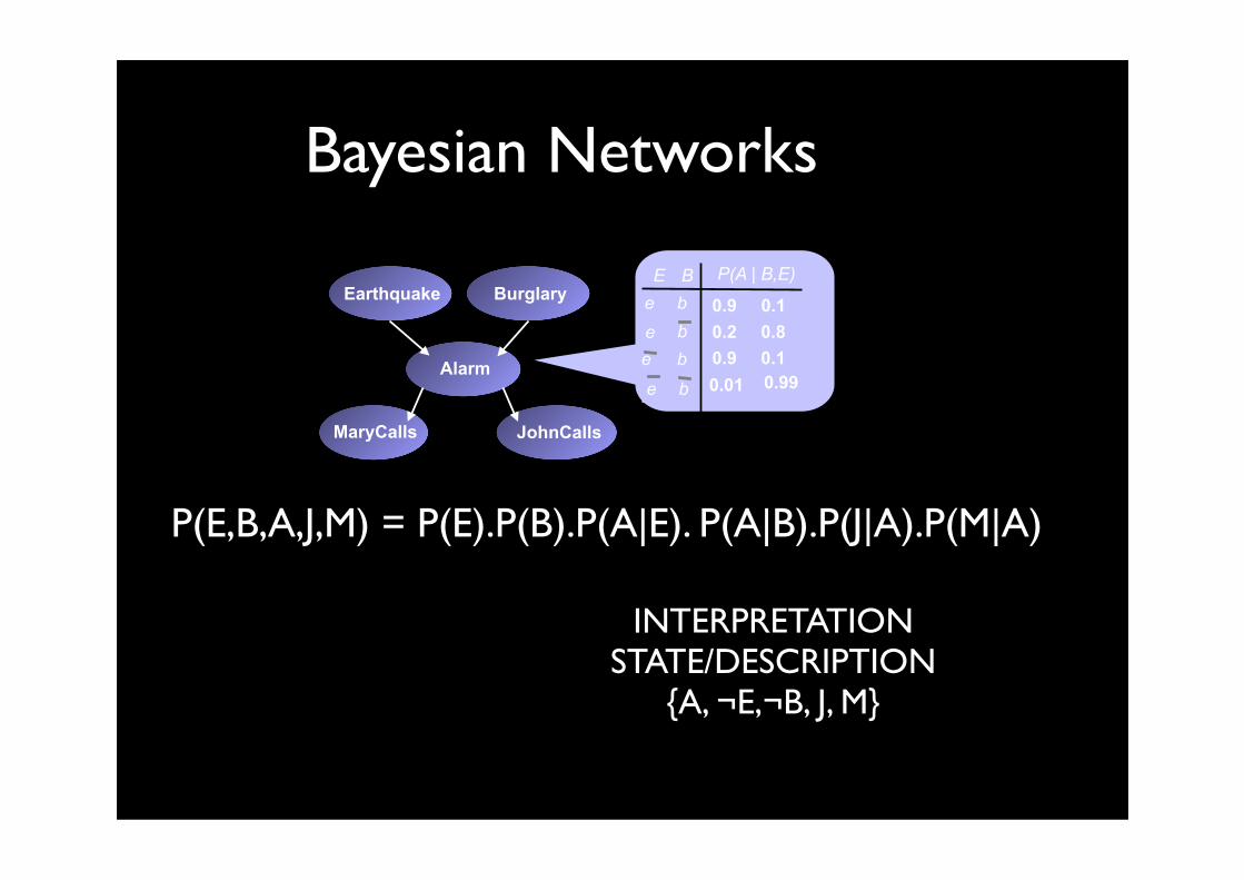
Bayesian Networks
0.9 0.1e
b
e0.2 0.8
0.01 0.990.9 0.1
bebb
e
BE P(A | B,E)Earthquake
JohnCalls
Alarm
MaryCalls
Burglary
P(E,B,A,J,M) = P(E).P(B).P(A|E). P(A|B).P(J|A).P(M|A)
INTERPRETATIONSTATE/DESCRIPTION
{A, ¬E,¬B, J, M}

missing value
hidd
en/
late
nt
Parameter Estimation
A1 A2 A3 A4 A5 A6
true true ? true false false
? true ? ? false false
... ... ... ... ... ...
true false ? false true ?
incomplete data setReal-world data: states of some random
variables are missing– E.g. medical diagnose: not
all patient are subjects to all test
– Parameter reduction, e.g. clustering, ...

Parameter Estimation: EM Idea
• In the case of complete data, ML parameter estimation is easy:
– simply counting (1 iteration)
Incomplete data ?
1. Complete data (Imputation)
• most probable?, average?, ... value2. Count
3. Iterate

EM Idea: Complete the dataincomplete data
A B
true true
true ?
false true
true false
false ?
complete data
0.8
1.2
1.4
1.6
N
falsefalse
truefalse
falsetrue
truetrue
BA
expected counts
P B = true A = false( ) = 0.2
P B = true A = true( ) = 0.6
B=true A=true =
1.61.6 +1.4
= 0.54
B=true A= false =
1.21.2 + 0.8
= 0.6
A B
complete
iterate

Learning Bayesian Networks
Two issues
• parameters (EM or gradient)
• structure (traverse a search space; very much like ILP; start from a DAG, and apply operations + scoring function)
Idea can be upgraded ...
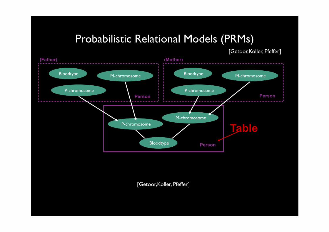
Probabilistic Relational Models (PRMs)
PersonBloodtype
M-chromosomeP-chromosome
Person
Bloodtype M-chromosome
P-chromosome
(Father)
Person
Bloodtype M-chromosome
P-chromosome
(Mother)
Table
[Getoor,Koller, Pfeffer]
[Getoor,Koller, Pfeffer]

Probabilistic Relational Models (PRMs)
bt(Person,BT).
pc(Person,PC).
mc(Person,MC).
bt(Person,BT) :- pc(Person,PC), mc(Person,MC).
pc(Person,PC) :- pc_father(Father,PCf), mc_father(Father,MCf).
pc_father(Person,PCf) | father(Father,Person),pc(Father,PC)....
father(Father,Person).
PersonBloodtype
M-chromosomeP-chromosome
Person
Bloodtype M-chromosome
P-chromosome
(Father)
Person
Bloodtype M-chromosome
P-chromosome
(Mother)
View :
Dependencies (CPDs associated with):
mother(Mother,Person).[Getoor,Koller, Pfeffer]

Probabilistic Relational Models (PRMs)Bayesian Logic Programs (BLPs)
father(rex,fred). mother(ann,fred). father(brian,doro). mother(utta, doro). father(fred,henry). mother(doro,henry).
bt(Person,BT) | pc(Person,PC), mc(Person,MC).pc(Person,PC) | pc_father(Person,PCf), mc_father(Person,MCf).mc(Person,MC) | pc_mother(Person,PCm), pc_mother(Person,MCm).
mc(rex)
bt(rex)
pc(rex)mc(ann) pc(ann)
bt(ann)
mc(fred) pc(fred)
bt(fred)
mc(brian)
bt(brian)
pc(brian)mc(utta) pc(utta)
bt(utta)
mc(doro) pc(doro)
bt(doro)
mc(henry)pc(henry)
bt(henry)
RV State
pc_father(Person,PCf) | father(Father,Person),pc(Father,PC)....
Extension
Intension

Answering Queries
mc(rex)
bt(rex)
pc(rex)mc(ann) pc(ann)
bt(ann)
mc(fred) pc(fred)
bt(fred)
mc(brian)
bt(brian)
pc(brian)mc(utta) pc(utta)
bt(utta)
mc(doro) pc(doro)
bt(doro)
mc(henry)pc(henry)
bt(henry)
P(bt(ann)) ? Support Network

Answering Queries
mc(rex)
bt(rex)
pc(rex)mc(ann) pc(ann)
bt(ann)
mc(fred) pc(fred)
bt(fred)
mc(brian)
bt(brian)
pc(brian)mc(utta) pc(utta)
bt(utta)
mc(doro) pc(doro)
bt(doro)
mc(henry)pc(henry)
bt(henry)
P(bt(ann), bt(fred)) ?
P(bt(ann)| bt(fred)) =
P(bt(ann),bt(fredP(bt(fred
Bayes‘ rule

Combining Rules
Students reads two books
Typical, noisy-or, noisy-max,
... P(A|B,C)
P(A|B) and P(A|C)
prepared(Student,Topic) | read(Student,Book),
discusses(Book,Topic).
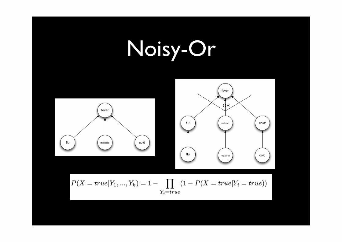
Noisy-Or
fever
flu malaria cold
fever
flu' malaria' cold'
flumalaria cold
OR

Knowledge Based Model Construction
Extension + Intension =>Probabilistic Model
Advantages
same intension used for multiple extensions
parameters are being shared / tied together
unification is essential
•learning becomes feasible
• Typical use includes
•prob. inference P(Q | E), P(bt(mary) | bt(john) =o-)
•max. likelihood parameter estimation & structure learning

Bayesian Logic Programs
% apriori nodesnat(0).
% aposteriori nodesnat(s(X)) | nat(X).
nat(0) nat(s(0)) nat(s(s(0)) ...MC
% apriori nodesstate(0).
% aposteriori nodesstate(s(Time)) | state(Time).output(Time) | state(Time)
state(0)
output(0)
state(s(0))
output(s(0))
...HMM
% apriori nodesn1(0).
% aposteriori nodesn1(s(TimeSlice) | n2(TimeSlice).n2(TimeSlice) | n1(TimeSlice).n3(TimeSlice) | n1(TimeSlice), n2(TimeSlice).
n1(0)
n2(0)
n3(0)
n1(s(0))
n2(s(0))
n3(s(0))
...DBN
pure P
rolog
Prolog and Bayesian Nets as Special Case

Learning BLPs
RVs + States = (partial) Herbrand interpretationProbabilistic learning from interpretations
Family(1)pc(brian)=b,
bt(ann)=a,
bt(brian)=?,
bt(dorothy)=a
Family(2)bt(cecily)=ab,
pc(henry)=a,
mc(fred)=?,
bt(kim)=a,
pc(bob)=b
Backgroundm(ann,dorothy),
f(brian,dorothy),
m(cecily,fred),
f(henry,fred),
f(fred,bob),
m(kim,bob),
...
Family(3)pc(rex)=b,
bt(doro)=a,
bt(brian)=?
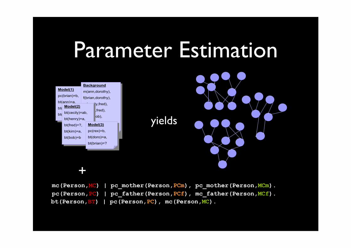
Parameter Estimation
+
bt(Person,BT) | pc(Person,PC), mc(Person,MC).pc(Person,PC) | pc_father(Person,PCf), mc_father(Person,MCf).mc(Person,MC) | pc_mother(Person,PCm), pc_mother(Person,MCm).
yields

Parameter Estimation
+
bt(Person,BT) | pc(Person,PC), mc(Person,MC).pc(Person,PC) | pc_father(Person,PCf), mc_father(Person,MCf).mc(Person,MC) | pc_mother(Person,PCm), pc_mother(Person,MCm).
yields
Parameter tying

Balios Tool
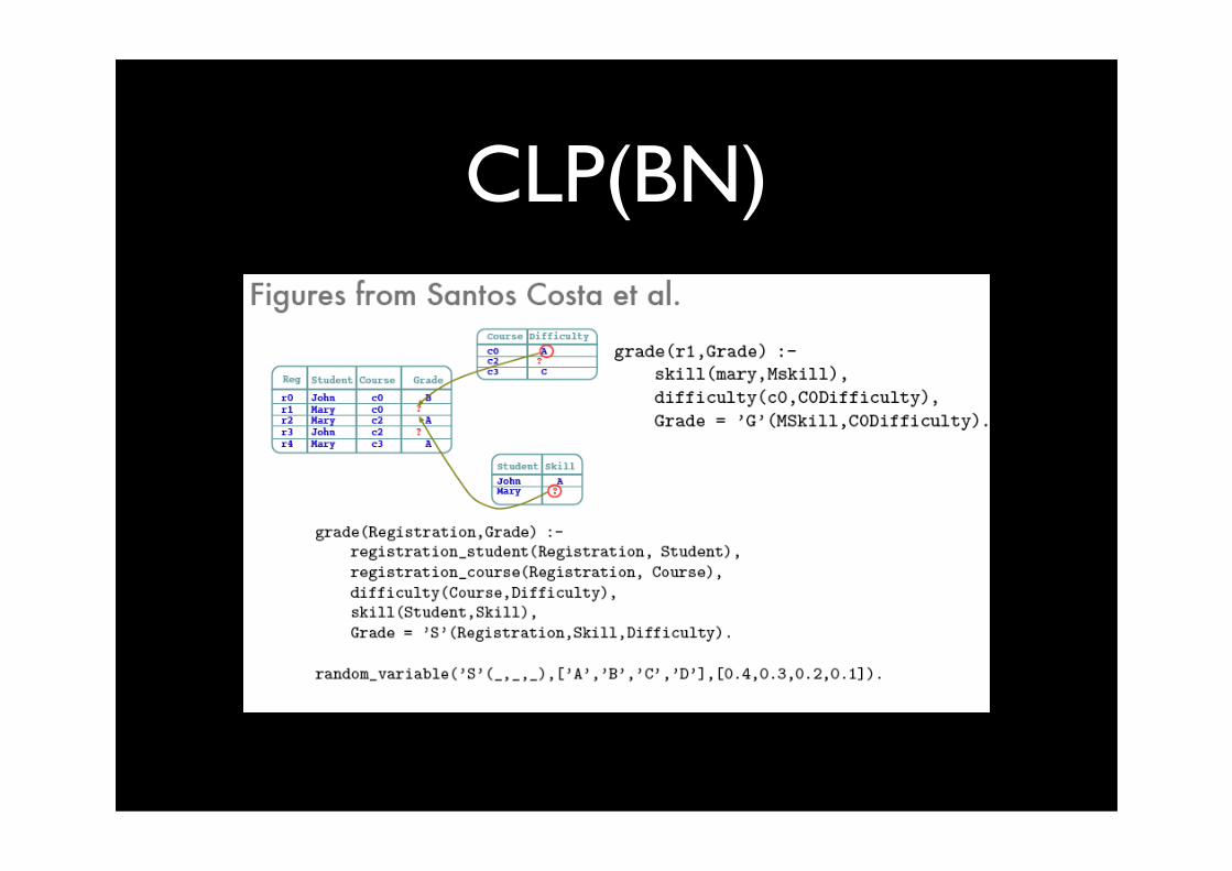
CLP(BN)

Markov Networks

Markov NetworkThe joint probability distribution P(X1, · · · , Xn) defined by a Markov net-
work factorizes as
P(X1, · · · , Xn) =1Z
!
c:clique
!c(Xc1, · · · , Xckc) (1)
where Z is a normalization constant needed to obtain a probability distribution(summing to 1). It is defined by
Z ="
x1,··· ,xn
!
c:clique
!c(Xc1 = xc1, · · ·, Xckc = xckc) (2)
P(B,E,A, J, M) =1Z
fA,E,B(A,E, B)! fA,J(A, J)! fA,M (A,M) (3)

Markov Network
The joint probability distribution P(X1, · · · , Xn) defined by a Markov net-work factorizes as
P(X1, · · · , Xn) =1Z
!
c:clique
!c(Xc1, · · · , Xckc) (1)
where Z is a normalization constant needed to obtain a probability distribution(summing to 1). It is defined by
Z ="
x1,··· ,xn
!
c:clique
!c(Xc1 = xc1, · · ·, Xckc = xckc) (2)
P(B,E,A, J, M) =1Z
exp(w1fA,E,B(A,E, B) + w2fA,J(A, J) + w3fA,M (A,M)) (3)

SELECT doc1.Category,doc2.Category
FROM doc1,doc2,Link link
WHERE link.From=doc1.key and link.To=doc2.key
Link
Doc1 Doc2
Relational Markov Networks
Cancer(A)
Smokes(A) Smokes(B)
Cancer(B)
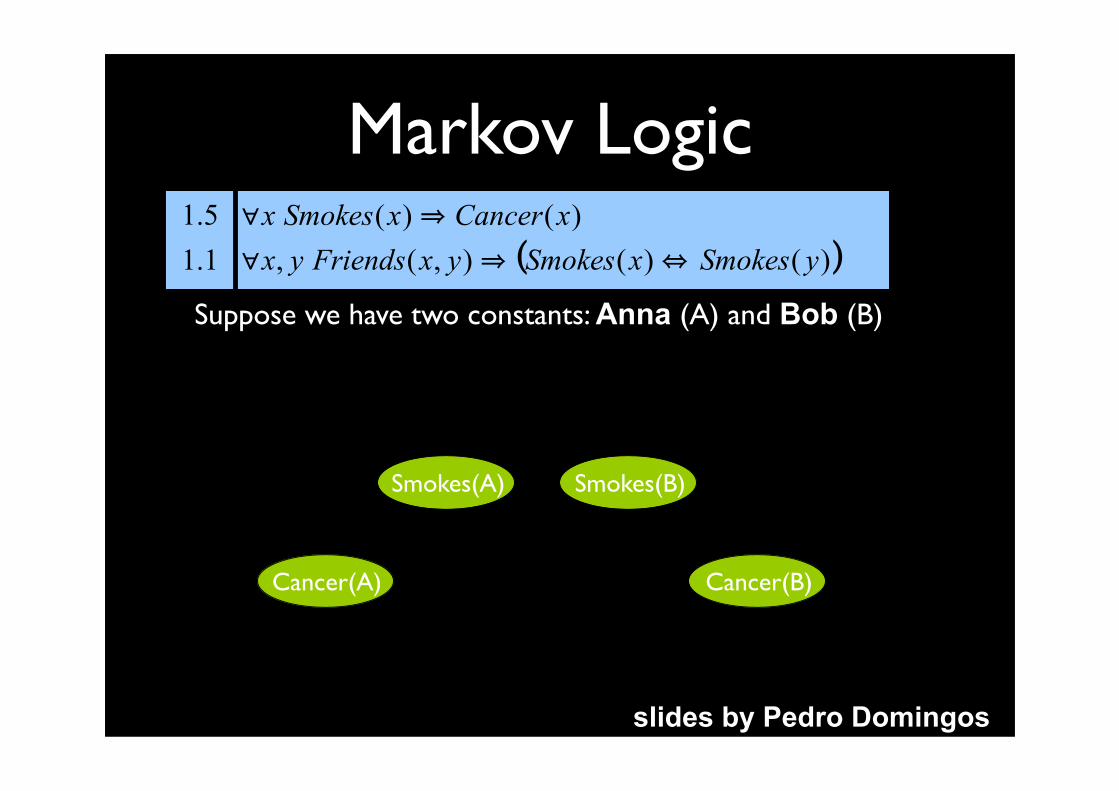
Suppose we have two constants: Anna (A) and Bob (B)
slides by Pedro Domingos
Markov Logic

Cancer(A)
Smokes(A)Friends(A,A)
Friends(B,A)
Smokes(B)
Friends(A,B)
Cancer(B)
Friends(B,B)
Suppose we have two constants: Anna (A) and Bob (B)
slides by Pedro Domingos
Markov Logic

Cancer(A)
Smokes(A)Friends(A,A)
Friends(B,A)
Smokes(B)
Friends(A,B)
Cancer(B)
Friends(B,B)
Suppose we have two constants: Anna (A) and Bob (B)
slides by Pedro Domingos
Markov Logic

Cancer(A)
Smokes(A)Friends(A,A)
Friends(B,A)
Smokes(B)
Friends(A,B)
Cancer(B)
Friends(B,B)
Suppose we have two constants: Anna (A) and Bob (B)
slides by Pedro Domingos
Markov Logic

Parameter estimation
• discriminative (gradient, max-margin)
• generative setting using pseudo-likelihood
Structure learning
• Similar to (Probabilistic) Inductive Logic Programming
Emphasis of work still on Inference
Learning Undirected Probabilistic Relational

Incorporates objects and relations among the objects into Bayesian and Markov networks
Data cases are Herbrand interpretations
Learning includes principles from
• Inductive logic programming / multi-relational data mining
• Refinement operators
• Background knowledge
• Bias
• Statistical learning
• Likelihood
• Independencies
• Priors
Conclusions Learning from Interpretations
LOGIC, RELATIONS and PROBABILITY
Probabilistic Logical Model
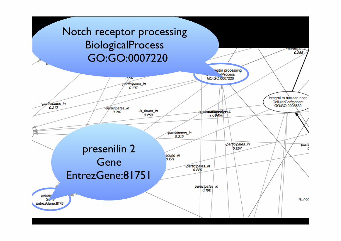
presenilin 2Gene
EntrezGene:81751
Notch receptor processingBiologicalProcessGO:GO:0007220

-participates_in0.220
BiologicalProcess
Gene

Network around Alzheimer Disease
gene
phenotype
probability of connection?
Two terminal network reliability problem [NP-hard]Work by Helsinki group Biomine project [Sevon, Toivonen et al. DILS 06]
Originally formulated as a probabilistic networkWe: upgrade towards probabilistic logic (ProbLog)

Distribution SemanticsDue to Taisuke Sato
• provides a natural basis for many probabilistic logics
• PRISM (Sato & Kameya), PHA & ICL (Poole), ProbLog (De Raedt et al.), CP-logic (Vennekens, ...)
• Will represent a simplified and unifying view as in ProbLog [De Raedt et al.]

Distribution Semantics• probabilistic predicates F
• define using p : q(t1,...,tn)
• denotes that ground atoms q(t1,...,tn)θ are true with probability p
• assume all ground probabilistic atoms to be marginally independent
• logical ones DB
• define as usual using logic program -- WE : PATH predicate
• a similar semantics has been reinvented many times ----

Distribution Semantics
Sato’s distribution semantics unifies the two elementary notions from logic and from probability theory
• a random variable = a ground atom, a proposition
And then uses logic for inference
• atomic choice + definite clause program -> minimal Herbrand model = possible world

Example in ProbLog
②
④
③
⑤⑥
AH
G
ED
F
C
B
①0.6
0.20.7
0.4
0.8
0.50.7
0.9
0.9 : y_edge(1,2).0.8 : r_edge(2,3).0.6 : g_edge(3,4)....ProbLog theory T
logical part L
facts mutually independent
[De Raedt, Kimmig, Toivonen, IJCAI 07]

Sampling Subprograms②
④
③
⑤⑥
AH
G
ED
F
C
B
①0.6
0.20.7
0.4
0.8
0.50.7
0.9
• Biased coins• Independent
②
④
③
⑤⑥
①
A B C D E F G H+ + + − − + − −
P = 0.9 · 0.8 · 0.6·(1! 0.5) · (1! 0.7) · 0.7·(1! 0.4) · (1! 0.2)
ABCF

②
④
③
⑤⑥
AH
G
ED
F
C
B
①0.6
0.20.7
0.4
0.8
0.50.7
0.9
Queries
①→④
P (q|T ) =!
S!L,S|=q
P (S|T )...
path(x,y) :- edge(x,y)path(x,y) :- edge(x,z), path(y,z)

②
④
③
⑤⑥
AH
G
ED
F
C
B
①0.6
0.20.7
0.4
0.8
0.50.7
0.9
Queries
①→④
P (q|T ) =!
S!L,S|=q
P (S|T )
path(x,y) :- edge(x,y)path(x,y) :- edge(x,z), path(y,z)
Key Point of ProbLog and Logic
any relation can be defined

Query Probabilityusing proofs
②
④
③
⑤⑥
AH
G
ED
F
C
B
①0.6
0.20.7
0.4
0.8
0.50.7
0.9①→④ABCABEHADGHADGEC
FGHFGECFDBCFDBEH
P (path(1, 4)|T )= P (ABC + ABEH + . . . + FDBEH)
• proofs overlap• disjoint sum•NP-hard• approximation algorithm
[De Raedt et al, IJCAI 07]

Query Probabilityusing Proofs
②
④
③
⑤⑥
AH
G
ED
F
C
B
①0.6
0.20.7
0.4
0.8
0.50.7
0.9
Prism (Sato) and PHA (Poole) avoid the disjoint problem by requiring that
explanations do not overlap

example①→④
Most likely proof /explanation
②
④
③
⑤⑥
AH
G
ED
F
C
B
①0.6
0.20.7
0.4
0.8
0.50.7
0.9
② ④③A CB①0.9 0.60.8
ABC
Abduction

PRISM [Sato 95]btype(Btype) ← gtype(Gf, Gm), pgtype(Btype, Gf, Gm)
gtype(Gf, Gm) ← gene(mother, Gf), gene(father, Gm)pgtype(X, X, X) ← pgtype(X, X, Y) ← dominates(X, Y)pgtype(X, Y, X) ← dominates(X, Y)pgtype(ab, a, b) ← pgtype(ab, b, a) ← dominates(a, o) ← dominates(b, o) ←
Explanations (Abduction !) BK U H |= btype(o)
gene(m, a), gene(f, a) with probability 0.3 X 0.3 = 0.09gene(m, a), gene(f, o) with probability 0.3 X 0.55 = 0.165gene(m, o), gene(f, a) with probability 0.55 X 0.3 = 0.165
So, the probability of the atom bloodtype(a) = 0.09 + 0.165 + 0.165 = 0.42.
disjoint(0.3 : gene(P, a); 0.15 : gene(P, b); 0.55 : gene(P, o))

Learning in PRISM
[1995] : Taisuke Sato introduces EM-algorithm for PRISM; many further refinements and optimizations since then
Input to the system (learning from entailment)
• set of facts btype(o), btype(a), ....
• unobserved: probabilities of facts / disjoint statements / switches; have to be estimated
Very efficient: for many classes of programs (PCFG, PolyTree, HMMs, ...) Prism’s learning algorithm implements the standard ones (inside-outside, Baum-Welsh, ...) !

Distribution SemanticsSemantics ProbLog not really new, rediscovered many times
Intuitively, a probabilistic database
Formally, a distribution semantics [Sato 95]
Other systems, such as Sato’s Prism and Poole’s PHA avoid the disjoint sum problem
• assume that explanations / proofs are mutually exclusive, that is,
• P(A v B v C) = P(A) + P(B) + P(C)
Long term vision: develop an optimized probabilistic Prolog implementation in which other SRL formalisms can be compiled. (work together with Vitor Santos Costa and Bart Demoen, integration in YAP Prolog)

CP-logic [Vennekens et al. ]
Model domain as set of probabilistic causal laws:
Property φ causes some non-deterministic event, which has possible outcome Ai with probability pi.
E.g., “throwing a rock at a glass breaks it with probability 0.3 and misses it with probability 0.7”
(Broken(G):0.3) ∨ (Miss:0.7) ← ThrowAt(G).
Note that the actual non-deterministic event (“rock flying at glass”) is implicit
Slides CP-logic courtesy Joost Vennekens

Semantics:probability trees
State of domain~ logical interpretation
Transition to new state
•0.3
!!!!!!
!!!
0.7
"""""
""""
•0.5
!!!!!!
!!!
0.5
##
•
0.6
##
0.4
"""""
""""
• • • •
Transition prob.Non-deterministic
event
Prob. distr. over final states
Slides CP-logic courtesy Joost Vennekens

Semantics(Broken(G):0.3) ∨ (Miss:0.7)
← ThrowAt(G).•
0.3
!!!!!!
!!!
0.7
"""""
""""
• •
I |= ThrowAt(G)
I ! {Broken(G)} I ! {Miss}
Probability tree is an execution model of theory iff:
• Each tree-transition matches causal law• The tree cannot be extended
Slides CP-logic courtesy Joost Vennekens

Example
•
1John throws
!!•
0.6
Window breaks
""!!!!!!!!!!!!
0.4
doesn’t break
##""""""""""""
•
0.5
Mary throws
""!!!!!!!!!!!!
0.5doesn’t throw
!!
•
0.5
Mary throws
""!!!!!!!!!!!!
0.5doesn’t throw
!!•
0.8
Window breaks
""!!!!!!!!!!!!
0.2doesn’t break
!!
• •
0.8
Window breaks
""!!!!!!!!!!!!
0.2doesn’t break
!!
•
• • • •
(Break : 0.8)! Throws(Mary).(Break : 0.6)! Throws(John).
(Throws(Mary) : 0.5)! .
Throws(John)! .
P (Break) = 0.6 + 0.4 · 0.5 · 0.8 = 0.76Slides CP-logic courtesy Joost Vennekens

TheoremEach execution model defines the same probability
distribution over final states
•For a theory C, we denote the unique distribution generated by its execution models as πC
•This distribution πC can also be constructed using the well-founded model of the “instances” of C
Slides CP-logic courtesy Joost Vennekens

First-orderWe can use logical variables to represent blue-prints for classes of events, e.g.,
Each pit causes a breeze on each square
next to it with prob. α
!x, y (Breeze(x) : !) " NextTo(x, y) # Pit(y).!x (Breeze(x) : !) " #y NextTo(x, y) $ Pit(y).
For each square, being
next to (at least one) pit causes a breeze on it
with prob.α
2 α- α² α

Learning from ProofsProbabilistic Context Free Grammars
1.0 : S -> NP, VP1.0 : NP -> Art, Noun0.6 : Art -> a0.4 : Art -> the0.1 : Noun -> turtle0.1 : Noun -> turtles…0.5 : VP -> Verb0.5 : VP -> Verb, NP0.05 : Verb -> sleep0.05 : Verb -> sleeps….
The turtle sleeps
Art Noun Verb
NP VP
S
1
1 0.5
0.4 0.1 0.05
P(parse tree) = 1x1x.5x.1x.4x.05

PCFGsP (parse tree) =
!i pci
iwhere pi is the probability of rule iand ci the number of timesit is used in the parse tree
P (sentence) ="
p:parsetree P (p)
Observe that derivations always succeed, that isS ! T,Q and T ! R,Ualways yieldsS ! R,U, Q

Probabilistic DCG
1.0 S -> NP(Num), VP(Num)1.0 NP(Num) -> Art(Num), Noun(Num)0.6 Art(sing) -> a0.2 Art(sing) -> the0.2 Art(plur) -> the0.1 Noun(sing) -> turtle0.1 Noun(plur) -> turtles…0.5 VP(Num) -> Verb(Num)0.5 VP(Num) -> Verb(Num), NP(Num)0.05 Verb(sing) -> sleep0.05 Verb(plur) -> sleeps….
The turtle sleeps
Art(s) Noun(s) Verb(s)
NP(s) VP(s)
S
1
1 0.5
0.2 0.1 0.05
P(derivation tree) = 1x1x.5x.1x .2 x.05
Stochastic Logic ProgramsMuggleton, Cussens

In SLP notation
11
1/2
P(s([the,turtles,sleep],[])=1/6
1
1/3
1/2

Probabilistic DCGs
1.0 S -> NP(Num), VP(Num)1.0 NP(Num) -> Art(Num), Noun(Num)0.6 Art(sing) -> a0.2 Art(sing) -> the0.2 Art(plur) -> the0.1 Noun(sing) -> turtle0.1 Noun(plur) -> turtles…0.5 VP(Num) -> Verb(Num)0.5 VP(Num) -> Verb(Num), NP(Num)0.05 Verb(sing) -> sleep0.05 Verb(plur) -> sleeps….
The turtle sleeps
Art(s) Noun(s) Verb(s)
NP(s) VP(s)
S
1
1 0.5
0.2 0.1 0.05
P(derivation tree) = 1x1x.5x.1x .2 x.05
What about “A turtles sleeps” ?

Probabilistic DCGs
S -> NP(s), VP(s)NP(s) -> Art(s), Noun(s)Art(sing) -> theNoun(s) -> turtleVP(s) -> Verb(s)
The turtle sleeps
Art(s) Noun(s) Verb(s)
NP(s) VP(s)
S
1
1 0.5
0.2 0.1 0.05
P(derivation tree) = 1x1x.5x.1x .2 x.05
How to get the variables back ?
Learning from Proof Trees
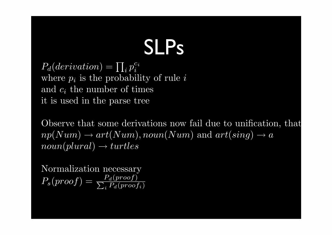
SLPsPd(derivation) =
!i pci
iwhere pi is the probability of rule iand ci the number of timesit is used in the parse tree
Observe that some derivations now fail due to unification, that isnp(Num)! art(Num), noun(Num) and art(sing)! anoun(plural)! turtles
Normalization necessaryPs(proof) = Pd(proof)P
i Pd(proofi)

Example Application• Consider traversing a university website• Pages are characterized by predicate
department(cs,nebel) denotes the page of cs following the link to nebel
• Rules applied would be of the form department(cs,nebel) :- prof(nebel), in(cs), co(ai), lecturer(nebel,ai). pagetype1(t1,t2) :- type1(t1), type2(t2), type3(t3), pagetype2(t2,t3)
• SLP models probabilities over traces / proofs / web logs department(cs,nebel), lecturer(nebel,ai007), course(ai007,burgard), …This is actually a Logical Markov Model
Logical Hidden Markov Model (cf. Kersting et al. JAIR)Includes also structured observations and abstraction
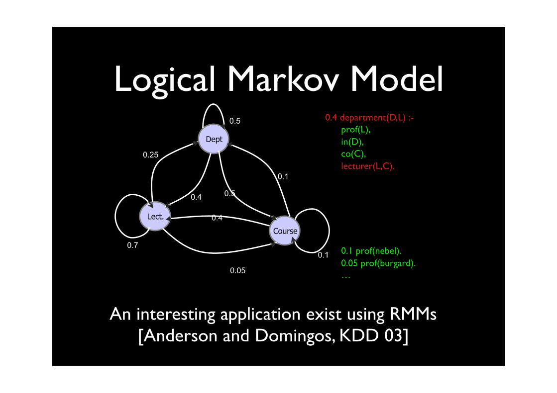
0.05
0.1
Lect.
Dept
Course
0.7
0.5
0.4
0.1
0.25
0.5
0.4
0.4 department(D,L) :-prof(L), in(D),co(C), lecturer(L,C).
0.1 prof(nebel).0.05 prof(burgard).…
Logical Markov Model
An interesting application exist using RMMs[Anderson and Domingos, KDD 03]
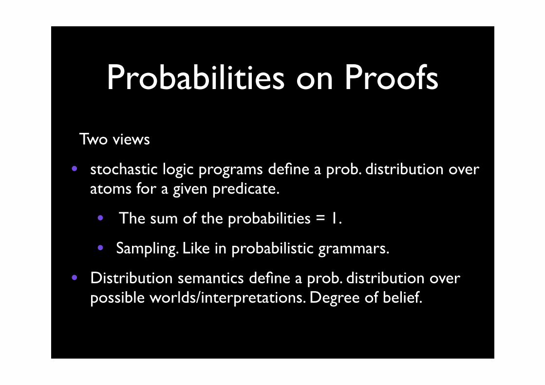
Probabilities on Proofs
Two views
• stochastic logic programs define a prob. distribution over atoms for a given predicate.
• The sum of the probabilities = 1.
• Sampling. Like in probabilistic grammars.
• Distribution semantics define a prob. distribution over possible worlds/interpretations. Degree of belief.

Probabilistic Programming LanguagesThere seems to be a trend towards extending multiple of these Probabilistic Logics towards Programming Languages,
• cf. NIPS-08 Workshop on Probabilistic Programming
• Various other paradigms involved as well, e.g. BLOG (Milch & Russell), IBAL (Pfeffer), Church (Goodmann et al. ), Dyna (Eisner), ...
• Should also allow to efficiently implement SRL systems

Dyna (Eisner et al.)
CKY Algorithm in Dyna constit(X,I,J) += rewrite(X,W) * word(W,I,J).constit(X,I,K) += rewrite(X,Y,Z) * constit(Y,I,J) * constit(Z,J,K).goal += constit(s,0,N) * end(N).
∑ Y,Z,J∑ W
Origins in Natural Language Processing ContextBased on Dynamic ProgrammingUseful for SRL/NLP/Programming
word(john,0,1), word(loves,1,2), word(Mary,2,3)0.003:: np -> Mary as rewrite(np,Mary)=0.0030.5::vp -> verb, np as rewrite(vp,verb,np)=0.5

Implementation Perspective
From an implementation perspective, the following languages are quite close:
• ProbLog, Prism, PHA, Prism
• CP-logic
• Stochastic Logic Programs
• CLP(BN) & BLP (to some degree)
Seems like one way out of the “Alphabet Soup”

TransformationsHave generated an alphabet soup of different languages, models and systems
The relationship is not always entirely clear
• though often statements like “my system can do whatever yours can” in paper with informal arguments
• if these statements are true
• differences are more a matter of elegance (syntactic sugar) than expressiveness ?
• the community may have wasted a lot of time on implementing variants,
• yet there are almost no usable SRL systems in the public domain today

TransformationsImplement a (primitive) probabilistic programming language (ProbLog, Dyna, ICL and Prism)
• primitives should be flexible enough to support key constructs in PP or SRL or PLL
• build optimized inference and learning engines for this language using state-of-the-art programming language & machine learning technology
Compile / transform other languages to this probabilistic programming language
Advantages should be clear.
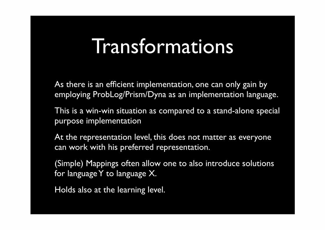
Transformations
As there is an efficient implementation, one can only gain by employing ProbLog/Prism/Dyna as an implementation language.
This is a win-win situation as compared to a stand-alone special purpose implementation
At the representation level, this does not matter as everyone can work with his preferred representation.
(Simple) Mappings often allow one to also introduce solutions for language Y to language X.
Holds also at the learning level.

REINFORCEMENT LEARNING

Markov Decision Process (MDP)MDP M = < S, A, T, R >
where
S: Finite set of states {s1,s2,…,sn}
A: Finite set of actions {a1,a2,…ak}
T(s,a,s’): probability to make a transition to state s’ if action a is used in state s
R(s,a,s’): reward for making a transition from state s to state s’ by doing action a
(also possible: R(s,a) and R(s) )
s
s’
a
7 states1 terminal state
2 actions
Slide Courtesy Martijn Van Otterlo

s
s1s2
s3
s4
s7s6
s5
0.3aaa
a
bbb
0.1
0.5
0.30.1
0.6
0.1
Some PropertiesThe Markov Property:
The current state and action give all possible information for predicting to which next state the agent will step. So… it does not matter how the agent arrived at his current state. (otherwise partially observable, compare chess to poker):
• States can be terminal (absorbing). Chains of steps will not be continued. Modelled as T(s,a,s)=1 (for all a) and R(s,a,s)=0.
• γ is the discount factor.
Slide Courtesy Martijn Van Otterlo

Policies, Rewards and GoalsA deterministic policy π selects an action as a function of the current state
The goal of an agent is to maximize some performance criterion. Among several, the discounted infinite horizon optimality criterion is often used:
Discount factor γ weighs future rewards.
Now the goal is to find the optimal policy as:
G
Slide Courtesy Martijn Van Otterlo
G

Problem Setup & Possible Solutions
For MDP M = < S, A, T, R >, we have roughly two situations:
1) Decision-theoretic planning (DTP)
If one has full knowledge about T and R, the setting is called model-based, and one can use (offline) dynamic programming techniques to compute optimal value functions and policies.
2) Reinforcement Learning (RL)
If one does not know T and R, the setting is called model-free, and one has to interact (online) with the environment to get learning samples. This exploration enables one to learn similar value functions and policies as in the model-based setting.
Models (T and R) can sometimes be learned
Slide Courtesy Martijn Van Otterlo

Relational MDPs and Logical Abstraction
Relational MDP
States “=“ interpretations
e.g. {on(a,b),cl(a),on(b,floor)}
Actions = {move(a,floor)}
semantics
Logical Formalism
Predicates P
Domain D
Action Formalisms(e.g. STRIPS, PPDDL, SitCalc)
on(X,Y), cl(X), cl(Z)
X ≠ Y, Y ≠ Z, X ≠ Z
cl(X), cl(Y), on(X,Z)
X ≠ Y, Y ≠ Z, X ≠ Z
0.9:move(X,Y)
Value functions e.g.
ϕ 10, not ϕ 0
Reward Functions
Policies
syntax
Induction = LRL
Slide Courtesy Martijn Van Otterlo

Search in unknown environment
Popular Algorithms
• Uninformed LRTA* [Koenig]
• Depth-first
Kersting et al. Advanced Rob. 07

222
Abstract states:
Abstract actions:
Abstract reward model:
Relational MDPs

Policy

224
Using a Relational Polichy
1. Start in State
2. Evaluate logical decision tree
3. Execute Action
4. Observe New State
5. Repeat if goal not yet reached.

move(X
,Y)
cl(X), cl(Y), on(X,Z), X ≠ Y, Y ≠ Z, X ≠ Z
and on(a,b) ≠ on(X,Y)
and on(a,b) ≠ on(X,Z)
a
b
X
Y Z
OWA
Regressionon(X,Y), cl(X), cl(Z)
X ≠ Y, Y ≠ Z, X ≠ Z
cl(X), cl(Y), on(X,Z)
X ≠ Y, Y ≠ Z, X ≠ Z
0.9:move(X,Y)
move(a,b)cl(a), cl(b), on(a,Z), a
≠ b, a ≠ Z, b ≠ Za
bZ
Match on(a,b) with on(X,Y)
a
b
Slide Courtesy Martijn Van Otterlo

Blocks world: on(a,b)V0:
10: on(a,b)
0 : true
γ = 0.9
actions: deterministic
Difficult for model-free Learners (e.g. RRL-TG)
Optimal for ±59M states
Slide Courtesy Martijn Van Otterlo
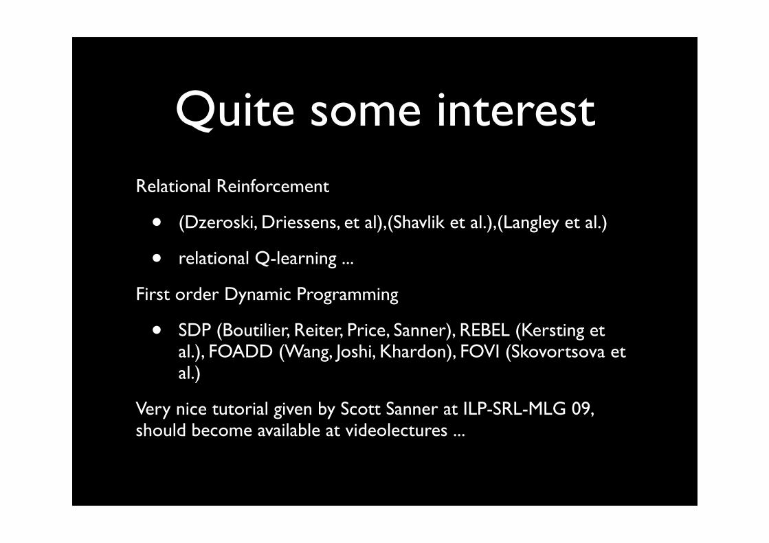
Quite some interestRelational Reinforcement
• (Dzeroski, Driessens, et al),(Shavlik et al.),(Langley et al.)
• relational Q-learning ...
First order Dynamic Programming
• SDP (Boutilier, Reiter, Price, Sanner), REBEL (Kersting et al.), FOADD (Wang, Joshi, Khardon), FOVI (Skovortsova et al.)
Very nice tutorial given by Scott Sanner at ILP-SRL-MLG 09, should become available at videolectures ...

Some Challenges LRLApplication challenges (social networks, robotics, dynamic situations)
Get the right level of representation / efficiency versus expressivity
Visualization of results (graphs - relations)
Theory of Statistical Relational Learning
Connection between relational representations and linear algebra
Learn at Theory Level (sets of interdependent predicates)
Predicate Invention
ConclusionsLogic and relational learning toolbox (take what you need)
• rules & background knowledge
• generality & operators
• upgrading & downgrading
• graphs & relational database & logic
• learning settings
• propositionalization & aggregation
• probabilistic logics

Further Reading
Luc De Raedt
Logical and Relational Learning
Springer, 2008, 401 pages.
(should be on display at the Springer booth)

Thanks to
Collaborators on previous tutorials, used slides, and specific aspects of this work, esp.
• Kristian Kersting, Angelika Kimmig, Hannu Toivonen, Joost Vennekens, Martijn van Otterlo, ...
![$1RYHO2SWLRQ &KDSWHU $ORN6KDUPD +HPDQJL6DQH … · 1 1 1 1 1 1 1 ¢1 1 1 1 1 ¢ 1 1 1 1 1 1 1w1¼1wv]1 1 1 1 1 1 1 1 1 1 1 1 1 ï1 ð1 1 1 1 1 3](https://img.pdfslide.us/doc/110x75/5f3ff1245bf7aa711f5af641/1ryho2swlrq-kdswhu-orn6kdupd-hpdqjl6dqh-1-1-1-1-1-1-1-1-1-1-1-1-1-1.jpg)


![1 1 1 1 1 1 1 ¢ 1 , ¢ 1 1 1 , 1 1 1 1 ¡ 1 1 1 1 · 1 1 1 1 1 ] ð 1 1 w ï 1 x v w ^ 1 1 x w [ ^ \ w _ [ 1. 1 1 1 1 1 1 1 1 1 1 1 1 1 1 1 1 1 1 1 1 1 1 1 1 1 1 1 ð 1 ] û w ü](https://img.pdfslide.us/doc/110x75/5f40ff1754b8c6159c151d05/1-1-1-1-1-1-1-1-1-1-1-1-1-1-1-1-1-1-1-1-1-1-1-1-1-1-w-1-x-v.jpg)

![arXiv:1511.07487v3 [cs.SI] 25 Feb 2016 · Arkaitz Zubiaga 1*, Maria Liakata , Rob Procter , Geraldine Wong Sak Hoi2, Peter Tolmie1 1 University of Warwick, Gibbet Hill Road, CV4 7AL](https://img.pdfslide.us/doc/110x75/600f8cd4d32dac70580f0362/arxiv151107487v3-cssi-25-feb-2016-arkaitz-zubiaga-1-maria-liakata-rob-procter.jpg)