Embed Size (px)
Citation preview

www.hydrosi.com
Prepared for: Montana Department of Environmental Quality Abandoned Mines Section Remediation Division 1520 East Sixth Avenue Helena, Montana 59620-0901
Under DEQ Contract No. 414026 – TO2
Prepared for: Abandoned Mines Section Remediation Division Montana Department of Environmental Quality 1520 East Sixth Avenue Helena, Montana 59620-0901
Prepared by: HydroSolutions Inc 4th Floor West 7 West 6th Avenue Helena, MT 59601 April 30, 2014
Final Report
Sand Coulee Acid Mine Drainage Groundwater Interception Investigation
Groundwater Interception Investigation April 30, 2014 DEQ Contract No. 414026 – TO2
HydroSolutions Inc i
Table of Contents
List of Figures ............................................................................................................................. ii
List of Appendices ....................................................................................................................... ii
1.0 Introduction ..................................................................................................................... 1
1.1 Task Descriptions ........................................................................................................ 1
1.2 Background.................................................................................................................. 2
2.0 Methods .......................................................................................................................... 4
2.1 Review of Wells and Mine Discharges ......................................................................... 4
2.2 Development of Geodatabase ..................................................................................... 4
2.3 Conceptual Model ........................................................................................................ 5
2.4 Horizontal Well Model Development ............................................................................ 7
2.4.1 HWELL Horizontal Well Model .............................................................................. 7
2.4.2 Dupuit-Forchheimer Model Development .............................................................. 8
2.4.3 Friction Loss ............................................................................................................... 9
2.5 AnAqSim Analytical Aquifer Model Development ........................................................10
2.5 Review of Applicable Geophysical Methods ................................................................12
3.0 Results and Discussion ..................................................................................................13
3.1 Well Inventory .............................................................................................................13
3.2 Geodatabase ..............................................................................................................14
3.3 Analytical Modeling Results and Comparisons ............................................................14
3.3.1 Horizontal Well Models ........................................................................................14
3.3.2 Vertical Well Model ...................................................................................................16
3.4 Application of Geophysical Methods ...........................................................................17
3.5 Preliminary Design and Feasibility of Drainage Well ...................................................20
4.0 Conclusions ....................................................................................................................23
6.0 References .....................................................................................................................25

Groundwater Interception Investigation April 30, 2014 DEQ Contract No. 414026 – TO2
HydroSolutions Inc ii
List of Tables Table 1. HWELL Model and Friction Loss Parameters ............................................................... 8
Table 2. Dupuit-Forchheimer Model Parameters ........................................................................ 9
Table 3. AnAqSim Model Parameters .......................................................................................12
Table 4. Summary of Geodatabase Components. .....................................................................14
Table 5. Discharge Results Horizontal Well Models ..................................................................15
Table 6. Results of Horizontal Well Model Sensitivity Analysis ..................................................16
Table 7. Simulated Reductions in Leakage to Gerber Mine by Vertical Drainage Wells ............17
List of Figures
Figure 1. Location of Study Area
Figure 2. Location of MBMG Wells and Mine Discharges within the Study Area
Figure 3. Conceptual Cross Section for Horizontal Well Design
Figure 4. Plan View of the Proposed Horizontal Well
Figure 5. Conceptual Cross Section for Vertical Well Design
Figure 6. AnAqSim Model Boundary Conditions
List of Appendices
Appendix A. Table of Groundwater Wells within the Sand Coulee Area (MBMG 2014)
Appendix B. File Geodatabase
Appendix C. Spreadsheet and Calculations of the Horizontal Well Models
Appendix D. AnAqSim Model Output

Groundwater Interception Investigation April 30, 2014 DEQ Contract No. 414026 – TO2
HydroSolutions Inc 1
Sand Coulee Acid Mine Drainage
Groundwater Interception Investigation Final Report
1.0 Introduction
The Sand Coulee Acid Mine Drainage Groundwater Interception Investigation Report is the result of a Task Order issued pursuant to DEQ Contract No. 414026 between HydroSolutions Inc. (HydroSolutions) and the Montana Department of Environmental Quality (DEQ). The purpose of the Task Order was to conduct an initial feasibility evaluation of both horizontal and vertical gravity drainage wells to reduce drainage from the Kootenai aquifer overlying the abandoned underground coal mines in the vicinity of Sand Coulee, Montana, in order to mitigate acid mine drainage (AMD). This work evaluated the concept of using gravity drainage wells to reduce AMD which was first investigated in the 1980’s research conducted by the Montana Bureau of Mines and Geology (MBMG) (Osborne et al. 1983; 1987). Comprehensive water quality investigations were completed in the Great Falls Coal Field by the U.S. Geological Survey (Karper 1998) and DEQ (Hydrometrics 2012). The start date of this Task Order was November 25, 2013. HydroSolutions identified a preliminary location to pilot test a horizontal drainage well and assessed the potential reduction in the volume of AMD discharging from nearby mines resulting from the drainage wells. The study area location is shown on Figure 1.
1.1 Task Descriptions
There were three tasks defined in Task Order 2 (TO2) and are described below. Task 1 – Compilation of Existing Data A comprehensive file geodatabase which incorporates the data generated by previous investigations conducted in the area was developed. The data includes interpolated elevation of the top of the coal seam, the interpolated groundwater potentiometric surface in the overlying Kootenai sandstone, and zones in the Kootenai sandstone where artesian conditions, water table conditions, and unsaturated conditions have been identified. Task 2 – Hydrogeologic Analysis The potential effectiveness of the pilot horizontal drainage well in reducing the amount of AMD discharging from nearby abandoned mines was analyzed using a Dupuit-Forchheimer model and the HWELL Horizontal Well Model (Haitjema, et al. 2010) (Beljin and Lasonsky 1992). A vertical drainage well was simulated using the analytical element model AnAqSim (Fitts GeoSolutions 2013). The analysis focused on estimating the yield of drainage wells and potential reduction in the amount of water discharging from the abandoned mine workings using drainage wells. The models incorporated the hydrogeology of the Sand Coulee area to the extent known from existing information. The applicability of geophysical methods to characterize

Groundwater Interception Investigation April 30, 2014 DEQ Contract No. 414026 – TO2
HydroSolutions Inc 2
the distribution of vertical and horizontal fractures in the Kootenai Formation and determine lateral limits of the abandoned mine workings was also assessed. Task 3 – Data Analysis and Reporting HydroSolutions used the geodatabase and the modeling results to evaluate the potential effectiveness and locations for drainage wells, and define general design parameters for the well, including anticipated length, borehole diameter, well construction materials, and approximate cost.
1.2 Background
The Sand Coulee Basin is located primarily in east-central Cascade County, southeast of the city of Great Falls. Bituminous coal occurs at the top of the Morrison Formation of the Jurassic Period. The coal deposit included iron-pyrite nodules up to 4-inches in diameter, which, during mining, were often discarded on the mine floor. Groundwater seeping through the coal and over the mine floor discharges from the former mine adits and is the primary source of AMD in the Sand Coulee area (Osborne et al. 1987). There are two sources of groundwater seeping into the abandoned mine workings:
• Infiltration from precipitation and snowmelt through the strata directly above the mine workings, and
• Groundwater originating from the regional flow system in the Kootenai aquifer. The hydrologic source control methods evaluated by the MBMG in the 1980’s were intended to reduce both of these sources, however, only the first control (infiltration reduction) was field tested. Field studies focused on a reduction in local infiltration to the coal mines by using intensified farming to control shallow recharge (Osborne et al. 1983; 1987). The use of horizontal or angled groundwater interception wells was discussed in the 1987 MBMG report, but no field testing took place due to lack of available directional drilling contractors. The Town of Sand Coulee is located in Section 13, T19N, R4E, as shown on Figure 1. A creek referred to as Rusty Ditch, Sand Coulee Fork, No Name Creek, and Straight Creek originates approximately 3.5 miles southwest of the town of Sand Coulee and flows northeast to its confluence with Sand Coulee Creek just north of Tracy. There are four abandoned coal mines that have continuous or intermittent discharges around Sand Coulee: The Gerber Mine, the Sand Coulee Mine, The Mount Oregon Mine, and the Nelson No. 1 Mine (Hydrometrics 2012). An inventory of abandoned mine features in the Sand Coulee area conducted in the early 1980s identified 30 mine waste dumps, approximately 40 subsidence depressions, 10 acid mine discharges, 10 open adits, 22 collapsed adits, and two open air shafts (Hydrometrics 1983). Reclamation work has been completed in the area by DEQ to mitigate the hazards posed by the abandoned mines, but AMD discharges have not been addressed. The most recent study indicates that total flow of AMD from the aforementioned abandoned mines has varied from approximately 14 gallons per minute (gpm) to 184 gpm depending on the time of year and antecedent precipitation (Hydrometrics 2012). Discharges from the abandoned mines to surface

Groundwater Interception Investigation April 30, 2014 DEQ Contract No. 414026 – TO2
HydroSolutions Inc 3
and groundwater have contaminated domestic wells and caused their abandonment as drinking water sources. Adverse effects of AMD have been observed at Sand Coulee for well over 100 years. By 1902, acid water drainage from the former Sand Coulee mine was reportedly polluted to the point that it was not suitable for industrial boiler use (Rossillon et al. 2009). All water quality studies conducted in the Great Falls coal field area over the past 40 years indicate the continuing severe water quality impacts caused by the AMD. Monthly water quality and streamflow data were collected at mine discharge sites within Sand Coulee from July 1994 through September 1996 and August 2011 to September 2012 (Karper 1998; Hydrometrics 2012). The discharge sites included Mining Gulch, Sand Coulee Mine, Oregon Mine at Kate’s Coulee, and Nelson Mine at Sand Coulee. The average pH of sampled mine discharge sites ranged from 2.6 to 3.1 (Hydrometrics 2012). The average concentrations of dissolved sulfate ranged from 2,633 to 10,562 mg/L, dissolved iron ranged from 284 to 1,525 mg/L, and dissolved aluminum ranged from 156 to 901 mg/L (Hydrometrics 2012). These levels exceed federal and Montana primary and secondary drinking water standards.

Groundwater Interception Investigation April 30, 2014 DEQ Contract No. 414026 – TO2
HydroSolutions Inc 4
2.0 Methods
Investigation procedures, field methods, and approaches for tasks completed as part of this investigation are organized and described in the following sections:
Section 2.1 Review of Wells and Mine Discharges Section 2.2 Development of Geodatabase Section 2.3 Conceptual Model Section 2.4 Horizontal Well Model Development Section 2.5 AnAqSim Well Model Development Section 2.5 Review of Applicable Geophysical Methods
2.1 Review of Wells and Mine Discharges
In 1984, the MBMG drilled monitoring wells within the Sand Coulee area. Eleven individual wells and nested well clusters were installed at sites overlying or generally southwest of the abandoned mines. The nested well sites have more than one monitoring well with varying completion depths. A field visit to Sand Coulee was performed on January 17, 2014 to visit the mine adit discharge locations and to locate the MBMG monitoring wells. The original locations of the MBMG monitoring wells in the 1987 report were based on topographic map locations (Osborne et al. 1987). Due to the uncertainty in the well locations, only two well clusters were located and identified, C-2 and C-6. The remaining well locations and conditions could be verified at a later date. The monitoring well and mine discharge locations are shown on Figure 2. The MBMG Groundwater Information Center (GWIC) online database was searched on January 15, 2014 for domestic and public water supply wells within the Sand Coulee Area. The area search included Sections 13, 14, 15, 21, 22, 23, 24, 25, 26, 27, 28, 33, 34, 35, T19N, R4E. The Department of Natural Resource and Conservation (DNRC) water rights online query system was searched on January 20, 2014 for the same area.
2.2 Development of Geodatabase
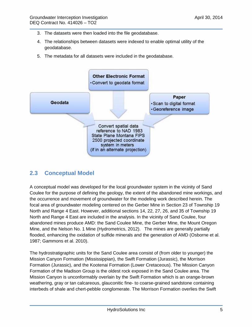
A file geodatabase was developed in the ArcGIS 10.2.1 desk top suite of software. The following list describes the data incorporation process.
1. Data sources were first evaluated to determine if their content was suitable for inclusion in the geodatabase.
2. The following diagram shows the steps taken to prepare different content types for inclusion in the geodatabase.
Groundwater Interception Investigation April 30, 2014 DEQ Contract No. 414026 – TO2
HydroSolutions Inc 5
3. The datasets were then loaded into the file geodatabase.
4. The relationships between datasets were indexed to enable optimal utility of the geodatabase.
5. The metadata for all datasets were included in the geodatabase.
2.3 Conceptual Model
A conceptual model was developed for the local groundwater system in the vicinity of Sand Coulee for the purpose of defining the geology, the extent of the abandoned mine workings, and the occurrence and movement of groundwater for the modeling work described herein. The focal area of groundwater modeling centered on the Gerber Mine in Section 23 of Township 19 North and Range 4 East. However, additional sections 14, 22, 27, 26, and 35 of Township 19 North and Range 4 East are included in the analysis. In the vicinity of Sand Coulee, four abandoned mines produce AMD: the Sand Coulee Mine, the Gerber Mine, the Mount Oregon Mine, and the Nelson No. 1 Mine (Hydrometrics, 2012). The mines are generally partially flooded, enhancing the oxidation of sulfide minerals and the generation of AMD (Osborne et al. 1987; Gammons et al. 2010). The hydrostratigraphic units for the Sand Coulee area consist of (from older to younger) the Mission Canyon Formation (Mississippian), the Swift Formation (Jurassic), the Morrison Formation (Jurassic), and the Kootenai Formation (Lower Cretaceous). The Mission Canyon Formation of the Madison Group is the oldest rock exposed in the Sand Coulee area. The Mission Canyon is unconformably overlain by the Swift Formation which is an orange-brown weathering, gray or tan calcareous, glauconitic fine- to coarse-grained sandstone containing interbeds of shale and chert-pebble conglomerate. The Morrison Formation overlies the Swift

Groundwater Interception Investigation April 30, 2014 DEQ Contract No. 414026 – TO2
HydroSolutions Inc 6
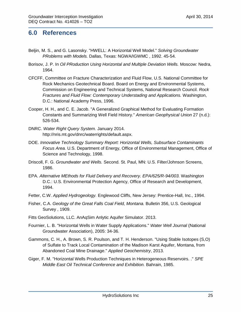
Formation and is mainly a greenish-gray mudstone and shale bed. The top 4 to 15 feet of the Morrison Formation is black shale and bituminous coal. The coal layer of the Morrison Formation is the bottom layer of the model. This unit is assumed to be confined. The Kootenai Formation unconformably overlies the Morrison Formation and is subdivided into five members (Kk1 – Kk5). The basal member (Kk1) forms the roof of the coal and serves as the historic source of potable water for the Sand Coulee Water District. Kk1 is mainly a crossbedded, moderately well-sorted quartz arenite with an average thickness of 30 feet in the modeled area. The Kk1 aquifer is confined southwest of the Sand Coulee Mine but becomes undefined and is partially dewatered approaching the up-gradient edge of the abandoned mines (Osborne et al. 1983). The Kk2 is predominantly a red mudstone which acts as an aquitard between the Kk1 and KK3. The KK3 is a well sorted resistant quartz arenite that is likely not an aquifer in the modeled area. The upper Kootenai units (Kk4 and Kk5) range from red mudstone, limestone, and sandstone and are unsaturated in the modeled area. The Kk4 and Kk5 were not part of the conceptual model design. The vertical gradients between the hydrostratigraphic unis are large because flow has to pass through the mudstone unit in the Kootenai (Kk2) which acts as an aquitard between the Kk3 and Kk1 (Osborne et al. 1983). The concept underlying this investigation is to intercept uncontaminated groundwater upgradient of the historic mine workings using gravity-driven drainage wells in the Kk1, and thereby reduce the leakage into and AMD emanating from the old mine workings. Two well designs were considered, a horizontal or low angle well, and a vertical drainage well. A horizontal well design may include some angle above or below the horizontal, but it is much closer to horizontal than to vertical in orientation, and would have to be installed using directional drilling technology. The vertical drainage well would be installed by a conventional water well contractor. The conceptual horizontal well is depicted in Figure 3. The Kk2 and Kk3 are modeled as one continuous unit. The horizontal well would be spudded at the lowest feasible elevation in Sand Coulee just upgradient (southwest) of the Gerber mine boundary. For the purpose of the current evaluation, the maximum practical horizontal well length was determined to be 1,500 feet in length (Lw) and 4 to 6 inches in diameter based on cost considerations and a review of available literature on horizontal well completions. The screened interval would be within the confined Kk1 and extend 500 feet. The potentiometric head of the Kk1 aquifer at the well screen was estimated to be 50-feet greater than the wellhead elevation based on historic potentiometric data (Osborne et al. 1987). A plan view topographic map of the proposed horizontal well is shown on Figure 4. The conceptual vertical drainage well is depicted in Figure 5. The well would be screened in the lower portion of the Kk1, cased through the Morrison and the Swift Formation, and completed as an open hole in the Mission Canyon Formation of the Madison Group. Since the hydraulic head of the Kk1 aquifer is anticipated to be approximately 200 feet greater than that of the Madison aquifer, groundwater would drain from the Kk1 into the underlying Madison aquifer. Similar to the horizontal well application, the objective is a reduction in the volume of groundwater available for leakage into the historic mine workings.
Groundwater Interception Investigation April 30, 2014 DEQ Contract No. 414026 – TO2
HydroSolutions Inc 7
2.4 Horizontal Well Model Development
Horizontal wells may offer an effective alternative to vertical wells, due to the greater screen length and aquifer contact. In certain favorable site conditions, horizontal wells can be used to produce groundwater to the surface using gravity-driven drainage. Steady-state two-dimensional (2-D) models have been developed for predicting groundwater withdrawal rates and capture zone delineation. Two mathematical models were used to estimate the discharge of a horizontal well drilled into the Kk1 and discharging at land surface without active pumping. The analysis was completed using a Dupuit-Forchheimer model and the HWELL Horizontal Well Model (Haitjema, et al. 2010) (Beljin and Lasonsky 1992). The development of the models is discussed in the following sections.
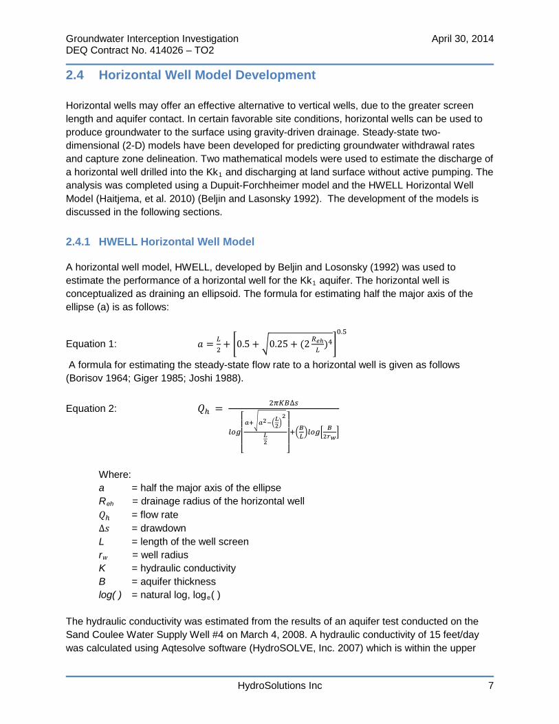
2.4.1 HWELL Horizontal Well Model A horizontal well model, HWELL, developed by Beljin and Losonsky (1992) was used to estimate the performance of a horizontal well for the Kk1 aquifer. The horizontal well is conceptualized as draining an ellipsoid. The formula for estimating half the major axis of the ellipse (a) is as follows:
Equation 1: 𝑎 = 𝐿2
+ �0.5 + �0.25 + (2 𝑅𝑒ℎ𝐿
)4�0.5
A formula for estimating the steady-state flow rate to a horizontal well is given as follows (Borisov 1964; Giger 1985; Joshi 1988).
Equation 2: 𝑄ℎ = 2𝜋𝐾𝐵∆𝑠
𝑙𝑜𝑔
⎣⎢⎢⎢⎡𝑎+�𝑎2−�𝐿2�
2
𝐿2
⎦⎥⎥⎥⎤
+�𝐵𝐿�𝑙𝑜𝑔�𝐵
2𝑟𝑤�
Where: a = half the major axis of the ellipse Reh = drainage radius of the horizontal well 𝑄ℎ = flow rate ∆𝑠 = drawdown L = length of the well screen rw = well radius K = hydraulic conductivity B = aquifer thickness log( ) = natural log, loge( )
The hydraulic conductivity was estimated from the results of an aquifer test conducted on the Sand Coulee Water Supply Well #4 on March 4, 2008. A hydraulic conductivity of 15 feet/day was calculated using Aqtesolve software (HydroSOLVE, Inc. 2007) which is within the upper
Groundwater Interception Investigation April 30, 2014 DEQ Contract No. 414026 – TO2
HydroSolutions Inc 8
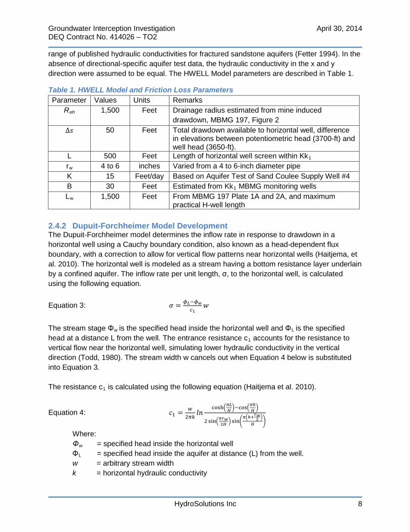
range of published hydraulic conductivities for fractured sandstone aquifers (Fetter 1994). In the absence of directional-specific aquifer test data, the hydraulic conductivity in the x and y direction were assumed to be equal. The HWELL Model parameters are described in Table 1.
Table 1. HWELL Model and Friction Loss Parameters Parameter Values Units Remarks
Reh 1,500 Feet Drainage radius estimated from mine induced drawdown, MBMG 197, Figure 2
∆𝑠 50 Feet Total drawdown available to horizontal well, difference in elevations between potentiometric head (3700-ft) and well head (3650-ft).
L 500 Feet Length of horizontal well screen within Kk1 rw 4 to 6 inches Varied from a 4 to 6-inch diameter pipe K 15 Feet/day Based on Aquifer Test of Sand Coulee Supply Well #4 B 30 Feet Estimated from Kk1 MBMG monitoring wells Lw 1,500 Feet From MBMG 197 Plate 1A and 2A, and maximum
practical H-well length 2.4.2 Dupuit-Forchheimer Model Development The Dupuit-Forchheimer model determines the inflow rate in response to drawdown in a horizontal well using a Cauchy boundary condition, also known as a head-dependent flux boundary, with a correction to allow for vertical flow patterns near horizontal wells (Haitjema, et al. 2010). The horizontal well is modeled as a stream having a bottom resistance layer underlain by a confined aquifer. The inflow rate per unit length, σ, to the horizontal well, is calculated using the following equation. Equation 3: 𝜎 = 𝜙𝐿−𝜙𝑤
𝑐1𝑤
The stream stage Φw is the specified head inside the horizontal well and ΦL is the specified head at a distance L from the well. The entrance resistance c1 accounts for the resistance to vertical flow near the horizontal well, simulating lower hydraulic conductivity in the vertical direction (Todd, 1980). The stream width w cancels out when Equation 4 below is substituted into Equation 3. The resistance c1 is calculated using the following equation (Haitjema et al. 2010).
Equation 4: 𝑐1 = 𝑤2𝜋𝑘
𝑙𝑛cosh�𝜋𝐿𝐻 �−cos�
𝜋ℎ𝐻 �
2 sin�𝜋𝑟𝑤2𝐻 �sin�𝜋�ℎ+𝑟𝑤2 �
𝐻 �
Where: Φw = specified head inside the horizontal well ΦL = specified head inside the aquifer at distance (L) from the well.
w = arbitrary stream width k = horizontal hydraulic conductivity
Groundwater Interception Investigation April 30, 2014 DEQ Contract No. 414026 – TO2
HydroSolutions Inc 9
L = any distance from the horizontal well with head ΦL
H = thickness of the aquifer h = well invert above the aquifer base rw = radius of the horizontal well
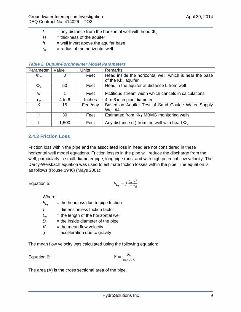
Table 2. Dupuit-Forchheimer Model Parameters Parameter Value Units Remarks
Φw 0 Feet Head inside the horizontal well, which is near the base of the Kk1 aquifer
ΦL 50 Feet Head in the aquifer at distance L from well
w 1 Feet Fictitious stream width which cancels in calculations rw 4 to 6 Inches 4 to 6 inch pipe diameter K 15 Feet/day Based on Aquifer Test of Sand Coulee Water Supply
Well #4 H 30 Feet Estimated from Kk1 MBMG monitoring wells
L 1,500 Feet Any distance (L) from the well with head ΦL 2.4.3 Friction Loss Friction loss within the pipe and the associated loss in head are not considered in these horizontal well model equations. Friction losses in the pipe will reduce the discharge from the well, particularly in small-diameter pipe, long pipe runs, and with high potential flow velocity. The Darcy-Weisbach equation was used to estimate friction losses within the pipe. The equation is as follows (Rouse 1946) (Mays 2001):
Equation 5: ℎ𝐿𝑓 = 𝑓 𝐿𝑤𝐷
𝑉2
2𝑔
Where: ℎ𝐿𝑓 = the headloss due to pipe friction 𝑓 = dimensionless friction factor
Lw = the length of the horizontal well D = the inside diameter of the pipe V = the mean flow velocity g = acceleration due to gravity
The mean flow velocity was calculated using the following equation:
Equation 6: 𝑉 = 𝑄ℎ86400𝐴
The area (A) is the cross sectional area of the pipe.
Groundwater Interception Investigation April 30, 2014 DEQ Contract No. 414026 – TO2
HydroSolutions Inc 10
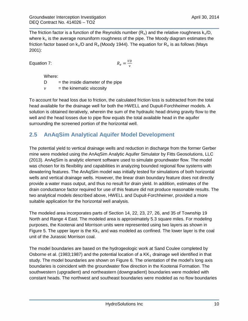
The friction factor is a function of the Reynolds number (Re) and the relative roughness ks/D, where ks is the average nonuniform roughness of the pipe. The Moody diagram estimates the friction factor based on ks/D and Re (Moody 1944). The equation for Re is as follows (Mays 2001): Equation 7: 𝑅𝑒 = 𝑉𝐷
𝜈
Where: D = the inside diameter of the pipe 𝜈 = the kinematic viscosity
To account for head loss due to friction, the calculated friction loss is subtracted from the total head available for the drainage well for both the HWELL and Dupuit-Forchheimer models. A solution is obtained iteratively, wherein the sum of the hydraulic head driving gravity flow to the well and the head losses due to pipe flow equals the total available head in the aquifer surrounding the screened portion of the horizontal well.
2.5 AnAqSim Analytical Aquifer Model Development
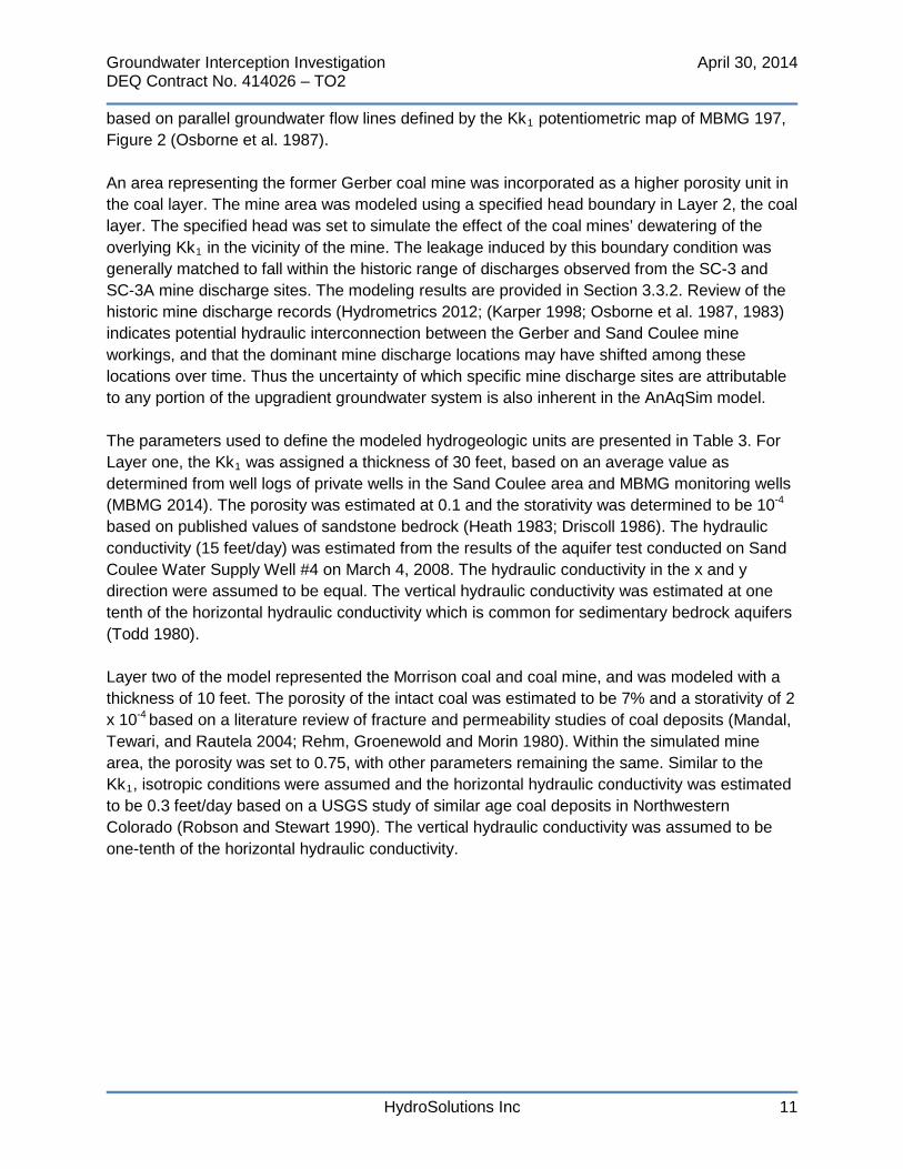
The potential yield to vertical drainage wells and reduction in discharge from the former Gerber mine were modeled using the AnAqSim Analytic Aquifer Simulator by Fitts Geosolutions, LLC (2013). AnAqSim is analytic element software used to simulate groundwater flow. The model was chosen for its flexibility and capabilities in analyzing bounded regional flow systems with dewatering features. The AnAqSim model was initially tested for simulations of both horizontal wells and vertical drainage wells. However, the linear drain boundary feature does not directly provide a water mass output, and thus no result for drain yield. In addition, estimates of the drain conductance factor required for use of this feature did not produce reasonable results. The two analytical models described above, HWELL and Dupuit-Forchheimer, provided a more suitable application for the horizontal well analysis. The modeled area incorporates parts of Section 14, 22, 23, 27, 26, and 35 of Township 19 North and Range 4 East. The modeled area is approximately 5.3 square miles. For modeling purposes, the Kootenai and Morrison units were represented using two layers as shown in Figure 5. The upper layer is the Kk1 and was modeled as confined. The lower layer is the coal unit of the Jurassic Morrison coal. The model boundaries are based on the hydrogeologic work at Sand Coulee completed by Osborne et al. (1983;1987) and the potential location of a KK1 drainage well identified in that study. The model boundaries are shown on Figure 6. The orientation of the model’s long axis boundaries is coincident with the groundwater flow direction in the Kootenai Formation. The southwestern (upgradient) and northeastern (downgradient) boundaries were modeled with constant heads. The northwest and southeast boundaries were modeled as no flow boundaries
Groundwater Interception Investigation April 30, 2014 DEQ Contract No. 414026 – TO2
HydroSolutions Inc 11
based on parallel groundwater flow lines defined by the Kk1 potentiometric map of MBMG 197, Figure 2 (Osborne et al. 1987). An area representing the former Gerber coal mine was incorporated as a higher porosity unit in the coal layer. The mine area was modeled using a specified head boundary in Layer 2, the coal layer. The specified head was set to simulate the effect of the coal mines’ dewatering of the overlying Kk1 in the vicinity of the mine. The leakage induced by this boundary condition was generally matched to fall within the historic range of discharges observed from the SC-3 and SC-3A mine discharge sites. The modeling results are provided in Section 3.3.2. Review of the historic mine discharge records (Hydrometrics 2012; (Karper 1998; Osborne et al. 1987, 1983) indicates potential hydraulic interconnection between the Gerber and Sand Coulee mine workings, and that the dominant mine discharge locations may have shifted among these locations over time. Thus the uncertainty of which specific mine discharge sites are attributable to any portion of the upgradient groundwater system is also inherent in the AnAqSim model. The parameters used to define the modeled hydrogeologic units are presented in Table 3. For Layer one, the Kk1 was assigned a thickness of 30 feet, based on an average value as determined from well logs of private wells in the Sand Coulee area and MBMG monitoring wells (MBMG 2014). The porosity was estimated at 0.1 and the storativity was determined to be 10-4 based on published values of sandstone bedrock (Heath 1983; Driscoll 1986). The hydraulic conductivity (15 feet/day) was estimated from the results of the aquifer test conducted on Sand Coulee Water Supply Well #4 on March 4, 2008. The hydraulic conductivity in the x and y direction were assumed to be equal. The vertical hydraulic conductivity was estimated at one tenth of the horizontal hydraulic conductivity which is common for sedimentary bedrock aquifers (Todd 1980). Layer two of the model represented the Morrison coal and coal mine, and was modeled with a thickness of 10 feet. The porosity of the intact coal was estimated to be 7% and a storativity of 2 x 10⁻⁴ based on a literature review of fracture and permeability studies of coal deposits (Mandal, Tewari, and Rautela 2004; Rehm, Groenewold and Morin 1980). Within the simulated mine area, the porosity was set to 0.75, with other parameters remaining the same. Similar to the Kk1, isotropic conditions were assumed and the horizontal hydraulic conductivity was estimated to be 0.3 feet/day based on a USGS study of similar age coal deposits in Northwestern Colorado (Robson and Stewart 1990). The vertical hydraulic conductivity was assumed to be one-tenth of the horizontal hydraulic conductivity.
Groundwater Interception Investigation April 30, 2014 DEQ Contract No. 414026 – TO2
HydroSolutions Inc 12
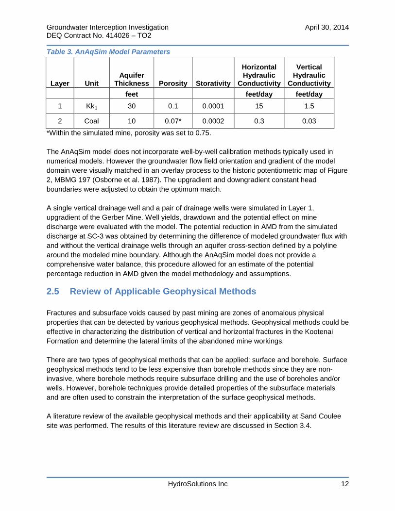
Table 3. AnAqSim Model Parameters
Layer Unit Aquifer
Thickness Porosity Storativity
Horizontal Hydraulic
Conductivity
Vertical Hydraulic
Conductivity feet feet/day feet/day 1 Kk1 30 0.1 0.0001 15 1.5
2 Coal 10 0.07* 0.0002 0.3 0.03 *Within the simulated mine, porosity was set to 0.75. The AnAqSim model does not incorporate well-by-well calibration methods typically used in numerical models. However the groundwater flow field orientation and gradient of the model domain were visually matched in an overlay process to the historic potentiometric map of Figure 2, MBMG 197 (Osborne et al. 1987). The upgradient and downgradient constant head boundaries were adjusted to obtain the optimum match. A single vertical drainage well and a pair of drainage wells were simulated in Layer 1, upgradient of the Gerber Mine. Well yields, drawdown and the potential effect on mine discharge were evaluated with the model. The potential reduction in AMD from the simulated discharge at SC-3 was obtained by determining the difference of modeled groundwater flux with and without the vertical drainage wells through an aquifer cross-section defined by a polyline around the modeled mine boundary. Although the AnAqSim model does not provide a comprehensive water balance, this procedure allowed for an estimate of the potential percentage reduction in AMD given the model methodology and assumptions.
2.5 Review of Applicable Geophysical Methods
Fractures and subsurface voids caused by past mining are zones of anomalous physical properties that can be detected by various geophysical methods. Geophysical methods could be effective in characterizing the distribution of vertical and horizontal fractures in the Kootenai Formation and determine the lateral limits of the abandoned mine workings. There are two types of geophysical methods that can be applied: surface and borehole. Surface geophysical methods tend to be less expensive than borehole methods since they are non-invasive, where borehole methods require subsurface drilling and the use of boreholes and/or wells. However, borehole techniques provide detailed properties of the subsurface materials and are often used to constrain the interpretation of the surface geophysical methods. A literature review of the available geophysical methods and their applicability at Sand Coulee site was performed. The results of this literature review are discussed in Section 3.4.

Groundwater Interception Investigation April 30, 2014 DEQ Contract No. 414026 – TO2
HydroSolutions Inc 13
3.0 Results and Discussion
The results of the groundwater interception investigation along with a discussion of the findings are organized and provided in the following sections:
Section 3.1 Well Inventory Section 3.2 Geodatabase Section 3.3 Analytical Modeling Results and Comparisons
Section 3.4 Application of Geophysical Methods Section 3.5 Preliminary Design and Feasibility of Drainage Well
3.1 Well Inventory
The status and location of all the MBMG monitoring wells at Sand Coulee could not be verified within the scope of this project. The approximate locations of the MGMG monitoring wells based on MBMG 197 are shown on Figure 2. The GWIC water well search provided 84 wells located within the queried sections of Sand Coulee and are presented in Appendix A. The results are sorted by aquifer of completion and section. The results included 47 domestic wells, 1 irrigation well, 10 public water supply wells, 14 MBMG research wells, 9 stockwater wells, and 3 wells of unknown use. There were 2 wells identified as being completed in the Alluvium, 36 wells completed in the Kootenai Formation, 37 wells completed in the Madison Formation, and 7 wells completed in the Morrison Formation. Wells completed in the Kootenai were not broken out as to which geologic member of the Kootenai Formation they were completed. Of the 36 wells completed in the Kootenai Formation, 10 of the wells were the MBMG research wells and 4 of the wells are Sand Coulee water supply wells. A new Sand Coulee water supply well was completed in the deeper Madison Formation in 2012 and is in the process of water right approval with the DNRC. After approval, the Sand Coulee water supply would be obtained from the Madison Formation and the water supply wells completed in the Kootenai Formation would not be in use. There are 6 wells completed in the Kootenai Formation within a mile of the proposed drainage well location that could be potentially affected by drainage wells. These wells are located in Sections 23, 26, and 27. Additional analysis will need to be performed as to whether the drainage will affect the yield of existing wells and potential water rights. The Sand Coulee water supply wells completed in the Kootenai Formation are located more than a mile downgradient from the proposed drainage well location and are not likely to be affected by the drainage wells under consideration. Mine discharge sampling locations SC-1, SC-3 and SC-9 are shown on Figure 2. On the date of the project site visit, the flow at SC-9 was visually estimated to be about 30 gpm and the discharge at SC-1 was estimated between 5 and 10 gpm. There was no surface discharge at SC-3 at the time of the site visit. The minimum historical flow rates for SC-1 and SC-3 are at or
Groundwater Interception Investigation April 30, 2014 DEQ Contract No. 414026 – TO2
HydroSolutions Inc 14
near 0 gpm and the average historical flow rate for SC-1 and SC-3 are 18 and 49 gpm, respectively (Hydrometrics 2012). The flow rate for sampling locations SC-1, SC-3, and SC-9 during August/September 2011 was 65, 35, and 46 gpm, respectively (Hydrometrics 2012).
3.2 Geodatabase
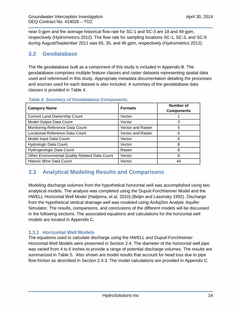
The file geodatabase built as a component of this study is included in Appendix B. The geodatabase comprises multiple feature classes and raster datasets representing spatial data used and referenced in this study. Appropriate metadata documentation detailing the processes and sources used for each dataset is also included. A summary of the geodatabase data classes is provided in Table 4.
Table 4. Summary of Geodatabase Components.
Category Name Formats Number of Components
Current Land Ownership Count Vector 1 Model Output Data Count Vector 3 Monitoring Reference Data Count Vector and Raster 5 Locational Reference Data Count Vector and Raster 6 Model Input Data Count Vector 6 Hydrologic Data Count Vector 8 Hydrogeologic Data Count Raster 8 Other Environmental Quality Related Data Count Vector 8 Historic Mine Data Count Vector 44
3.3 Analytical Modeling Results and Comparisons
Modeling discharge volumes from the hypothetical horizontal well was accomplished using two analytical models. The analysis was completed using the Dupuit-Forchheimer Model and the HWELL Horizontal Well Model (Haitjema, et al. 2010) (Beljin and Lasonsky 1992). Discharge from the hypothetical vertical drainage well was modeled using AnAqSim Analytic Aquifer Simulator. The results, comparisons, and conclusions of the different models will be discussed in the following sections. The associated equations and calculations for the horizontal well models are located in Appendix C.
3.3.1 Horizontal Well Models The equations used to calculate discharge using the HWELL and Dupuit-Forchheimer Horizontal Well Models were presented in Section 2.4. The diameter of the horizontal well pipe was varied from 4 to 6 inches to provide a range of potential discharge volumes. The results are summarized in Table 5. Also shown are model results that account for head loss due to pipe flow friction as described in Section 2.4.3. The model calculations are provided in Appendix C.

Groundwater Interception Investigation April 30, 2014 DEQ Contract No. 414026 – TO2
HydroSolutions Inc 15
Table 5. Results of Horizontal Well Models
Model 6 inch diameter
4 inch diameter
Model Results
Model Results including friction
loss Model Results
Model Results including friction
loss gpm
HWELL 269 225 267 138 Dupuit-
Forchheimer 108 104 108 86 The results indicate significant differences between the two analytical models for reasons based on the approach and assumptions of each. The HWELL model incorporates an elliptical capture zone centered on the well screen which includes groundwater capture both lateral to the well axis and beyond the ends of the well screen and does not simulate any resistance to vertical flow, leading to the greater predicted discharge rate compared to the Dupuit-Forchheimer Model. The Dupuit-Forchheimer Model simulates discharge to a horizontal well similarly to that of a linear stream feature, that is, from the groundwater regime flanking the well. The model results show little or no difference between the two well diameters evaluated. Pipe flow friction losses lead to reductions in discharge of from 4 – 16% for 6-inch diameter pipe, to reductions of 20 – 48% for 4-inch pipe. The HWELL model likely overestimates the potential discharge of a horizontal well for the hydrogeologic setting at Sand Coulee since the downgradient half of the hypothetical drainage ellipse is already partially dewatered by the abandoned mine. The upgradient side of the ellipse would contribute most of the well discharge and thus it is expected that the horizontal well envisioned by the conceptual model would have a steady state discharge of about one-half of the predicted HWELL model results in Table 5, closer to the results of the Dupuit-Forchheimer model. A sensitivity analysis was performed on several of the input parameters. The input parameters varied were hydraulic conductivity (K), the radius of influence or distance (L) to a specified head, and screen length. The results are presented in Table 6. The discharge is a linear function of the hydraulic conductivity for both the HWELL Model and Dupuit-Forchheimer Model. Increasing the radius of influence in the HWELL model or distance (L) in the Dupuit- Forchheimer model has the effect of decreasing the gradient to the well, and thus reducing the discharge. Reducing the screen length by one-half gives a modest reduction in discharge for the HWELL model and a proportionate reduction for the Dupuit-Forchheimer model.

Groundwater Interception Investigation April 30, 2014 DEQ Contract No. 414026 – TO2
HydroSolutions Inc 16
Table 6. Results of Horizontal Well Model Sensitivity Analysis
Model Adjusted
Parameter Adjusted
Value Discharge
(gpm) 6-inch Well
HWELL Original 269 HWELL K 1.5 ft/day 26.9 HWELL Radius of Influence 2,000 ft 243 HWELL Screen Length 250 ft 200 Dupuit-Forchheimer (D-F) Original 108
D-F K 1.5 ft/day 11 D-F Distance (L) 1,500 ft 74 D-F Screen Length 250 ft 54
4-inch Well HWELL Original 267 HWELL K 1.5 ft/day 26.7 HWELL Radius of Influence 2,000 ft 241 HWELL Screen Length 250 ft 197 Dupuit-Forchheimer (D-F) Original 108
D-F K 1.5 ft/day 11 D-F Distance (L) 1,500 ft 74 D-F Screen Length 250 ft 54
3.3.2 Vertical Well Model The Gerber Mine and associated Kk1 and coal aquifers were modeled using AnAqSim Analytic Aquifer Simulator by Fitts Geosolutions, LLC (2013), with input parameters, boundary conditions and modeling procedure as described in Section 2.5. The model elements are shown in Figure 6. A vertical well was placed near the location of MBMG monitoring well C-8. The drainage well was set with a constant head at the top of the Kk1 aquifer to simulate drawdown while maintaining confined conditions, and the total discharge of the well was computed by the model. The well effectively simulated a vertical drain in the Kk1 discharging to a highly transmissive interval in the underlying Mission Canyon Formation. The results of this analysis are located in Appendix D. The modeled volume of water draining into the Madison aquifer was 10,000 feet3/day or 52 gpm. A second vertical drainage well was added to the model, as presented in Appendix D, to assess the effects of multiple drainage wells on discharge from the simulated mine workings. The total combined discharge rate of the two wells to the Madison aquifer was 16,928 feet3/day or 88 gpm. Although AnAqSim does not directly provide water mass balances, an estimate of the reduction of leakage into the simulated Gerber mine workings was made by determining the flux
Groundwater Interception Investigation April 30, 2014 DEQ Contract No. 414026 – TO2
HydroSolutions Inc 17
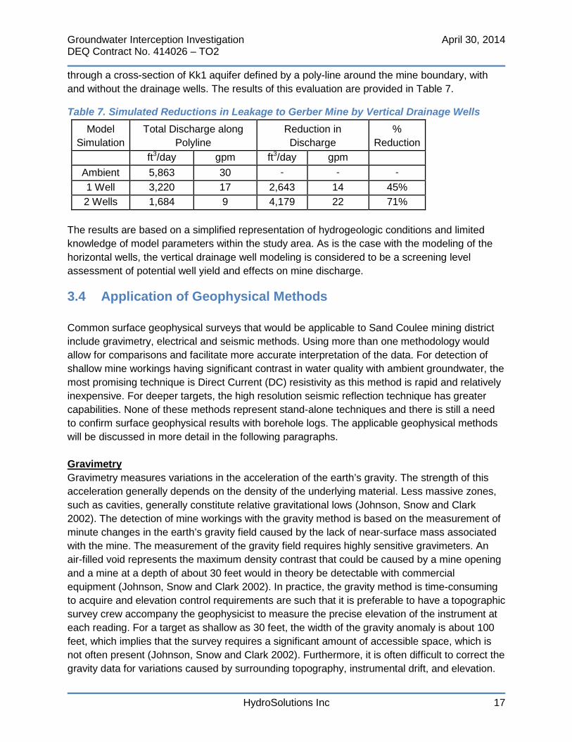
through a cross-section of Kk1 aquifer defined by a poly-line around the mine boundary, with and without the drainage wells. The results of this evaluation are provided in Table 7.
Table 7. Simulated Reductions in Leakage to Gerber Mine by Vertical Drainage Wells Model
Simulation Total Discharge along
Polyline Reduction in Discharge
% Reduction
ft3/day gpm ft3/day gpm
Ambient 5,863 30 - - - 1 Well 3,220 17 2,643 14 45% 2 Wells 1,684 9 4,179 22 71%
The results are based on a simplified representation of hydrogeologic conditions and limited knowledge of model parameters within the study area. As is the case with the modeling of the horizontal wells, the vertical drainage well modeling is considered to be a screening level assessment of potential well yield and effects on mine discharge.
3.4 Application of Geophysical Methods
Common surface geophysical surveys that would be applicable to Sand Coulee mining district include gravimetry, electrical and seismic methods. Using more than one methodology would allow for comparisons and facilitate more accurate interpretation of the data. For detection of shallow mine workings having significant contrast in water quality with ambient groundwater, the most promising technique is Direct Current (DC) resistivity as this method is rapid and relatively inexpensive. For deeper targets, the high resolution seismic reflection technique has greater capabilities. None of these methods represent stand-alone techniques and there is still a need to confirm surface geophysical results with borehole logs. The applicable geophysical methods will be discussed in more detail in the following paragraphs. Gravimetry Gravimetry measures variations in the acceleration of the earth’s gravity. The strength of this acceleration generally depends on the density of the underlying material. Less massive zones, such as cavities, generally constitute relative gravitational lows (Johnson, Snow and Clark 2002). The detection of mine workings with the gravity method is based on the measurement of minute changes in the earth’s gravity field caused by the lack of near-surface mass associated with the mine. The measurement of the gravity field requires highly sensitive gravimeters. An air-filled void represents the maximum density contrast that could be caused by a mine opening and a mine at a depth of about 30 feet would in theory be detectable with commercial equipment (Johnson, Snow and Clark 2002). In practice, the gravity method is time-consuming to acquire and elevation control requirements are such that it is preferable to have a topographic survey crew accompany the geophysicist to measure the precise elevation of the instrument at each reading. For a target as shallow as 30 feet, the width of the gravity anomaly is about 100 feet, which implies that the survey requires a significant amount of accessible space, which is not often present (Johnson, Snow and Clark 2002). Furthermore, it is often difficult to correct the gravity data for variations caused by surrounding topography, instrumental drift, and elevation.

Groundwater Interception Investigation April 30, 2014 DEQ Contract No. 414026 – TO2
HydroSolutions Inc 18
Unless the target is in a flat, open area and the depth does not exceed about 40-50 feet, the gravity method will probably not be practical. Electrical Electrical resistivity surveys tend to be reliable geophysical methods for identifying fractures or voids within the subsurface. Electrical resistivity is a volumetric property that describes the resistance of electrical current flow within a medium (HydroGeophysics 2009). Electrical methods measure changes in resistivity (opposite of conductivity). Sufficient background data is needed to distinguish the fractures or voids from the surrounding country rock. A fracture will not be identified if the variations in properties of the subsurface material surrounding the fracture are similar in contrast and scale to the fracture. A common electrical method is Direct Current (DC) resistivity surveys. The purpose of this method is to determine the subsurface resistivity distribution by making measurements over the ground surface. From these measurements, the resistivity of the subsurface can be estimated. The ground resistivity is related to various geological parameters such as the mineral and fluid content, porosity and degree of water saturation in the rock. The DC resistivity method would offer the best potential for rapidly mapping to a depth of 50 to 100 feet. This method would not be suitable for mapping to a greater than 100 feet and a different methodology or higher resolution resistivity method would need to be used. The maximum penetration depth is directly proportional to the electrode spacing and inversely proportional to the subsurface conductivity. DC resistivity can detect bulk anisotropy changes with depth and in some cases can be related to the dominant fracture direction at the site (Powers et al. 1999). The linear zones of low resistivity that are continuous with depth are interpreted as fracture zones. Resolution of fractures and precision in location are normally excellent if the fractures extend to the surface. However, in many cases, fractured bedrock is covered with overburden having electrical properties similar to those of the fracture zones. In practice, this limits resolution and may prevent detection of fractures or minor fracture zones. Electrical methods have been successful at determining subsurface lineations at other mine sites in Montana. An example of this geophysical application was at the Landusky Mine Site, 30 miles south of Malta, Montana, to delineate fractures hosting AMD) water (HydroGeophysics 2009). The depth to groundwater at this site was approximately 200 feet and the TDS of the AMD-affected groundwater ranged from 1800 to 6200 mg/L. Two electrical methods were applied to characterize the subsurface movement of AMD through fractures. High Resolution Resistivity (HRR) and Residual Potential Mapping (RPM) were used to create two dimensional profiles. HRR is a unique type of DC resistivity method that incorporates a higher data density per unit line length of the survey, maximum depth of investigation, higher signal to noise ratio, and less transmitted energy (HydroGeophysics 2009). Borehole geophysics was incorporated using the RPM method by transmitting electrical current through wells and measuring the voltage potential at a discrete location on the surface, which helped corroborate much of the interpretation resulting from the HRR method. The low resistivity results were interpreted as fractures hosting acidic groundwater. The methods employed were able to characterize the subsurface to a depth of 600 feet.

Groundwater Interception Investigation April 30, 2014 DEQ Contract No. 414026 – TO2
HydroSolutions Inc 19
At the Sand Coulee site, depth to groundwater is considerably less than that of the Landusky site, while the TDS of the AMD-impacted water is greater, ranging from 4,000 to 5,000 mg/L. Based on the shallower depths to groundwater and high degree of contrast between AMD-impacted and ambient groundwater, it is believed that HRR and RPM would be appropriate methods for subsurface mapping of impacted groundwater. However, it is less likely that these methods would be capable of mapping preferential groundwater flow paths within the fractures of the Kk1 upgradient of the contaminated zones which have a much lower TDS. Seismic The seismic reflection method works well for correlation with the DC resistivity method and for depths greater than 100 feet. Seismic is the technique most commonly used for deep subsurface imaging. The seismic techniques consist of measuring the travel time required for a seismic wave generated at or near the surface to return to surface or near-surface detectors (geophones) after reflection or refraction from acoustic interfaces between subsurface horizons (Johnson, Snow and Clark 2002). The seismic reflection method is the most powerful of all geophysical techniques in mapping subsurface layering but it is relatively costly. Nevertheless, the method offers the possibility to define subsurface structure beyond the ability of other methods. There should be a strong reflection on a void or large fracture encountered (Johnson, Snow and Clark 2002). The method has been successfully applied to the mapping of mine voids, but the experience base is limited and few practitioners have the skills to properly conduct this type of survey. Seismic results generally produce large data sets and extensive data processing is required to extract useful information. Anomalies may occur for a number of other reasons that may not involve fractures, but may falsely be interpreted as fractures (CFCFF 1996). Borehole Borehole geophysics provide access to measurement points below the ground surface, allowing many of the problems introduced by the overburden to be avoided. For most surface characterization techniques, overburden introduces difficulties because of its attenuation properties and the high contrast in its properties compared to the underlying rock. In many cases the overburden acts as a filter that obscures information about the deeper targets of interest, requiring the use of complex correction procedures to obtain useful information. The main advantage of combining borehole geophysics with surface geophysics is to provide subsurface confirmation of the surface measurements. They also allow surface measurements to be tied directly to lithology and structure. Borehole investigations are also more costly than comparable surface surveys, owing to higher drilling and measurement costs (CFCFF 1996). Incorporation of borehole geophysics into already planned exploration drilling or monitoring well programs is often cost effective. The availability of borehole imaging methods for subsurface fracture and void identification and other geophysical logs for fracture characterization provides effective methods for describing fractures that intersect exploratory boreholes. However, this near-borehole data does not

Groundwater Interception Investigation April 30, 2014 DEQ Contract No. 414026 – TO2
HydroSolutions Inc 20
provide useful information about connections between fractures and the larger-scale groundwater flow systems (CFCFF 1996).
3.5 Preliminary Design and Feasibility of Drainage Well
A proposed approximate wellhead location of a pilot horizontal well is shown on Figure 2. The legal description is the SE1/4, NE1/4, SW1/4, Section 23, T19N, R4E, or approximately 1.2 miles southeast of the town of Sand Coulee. Any actual location of a well would be based on accessibility, landowner agreements, and the results of a detailed hydrogeologic site investigation. The total well length was selected to be 1,500 feet with a screened interval of 500 feet based on current research into maximum practical horizontal well lengths (Fournier 2005). The horizontal well would have a pipe diameter of 4 to 6 inches, to be determined based on actual site conditions, contractor capabilities and costs. The average horizontal well is more expensive and technically more difficult to drill and install than the average vertical well. Based on drilling cost statistics from the United States oil and gas industry, horizontal wells cost 1.5 to 2.5 times more than a vertical well (Joshi 2003). Alternately, horizontal wells are a proven technology originally developed in the 1920’s and have been used for a variety of applications (Hunt 2002). Horizontal drilling technology began to be widely used for subsurface utility installations in the 1970’s. By the late 1980s, horizontal well technology was being applied to environmental remediation (Kaback 2002). Currently, horizontal wells have widespread use and development in the oil and gas industry, and therefore, the drilling technology is decreasing in cost over time. There are two different types of horizontal wells, continuous and blind wells. Continuous wells have both an entry and exit hole. Continuous well bores are typically used in shallow applications such as installing utilities under water bodies, roadways, or buildings, and for environmental remediation wells (Williams 2008). Continuous wells are typically installed by drilling surface to surface. Well materials are then pulled from the exit hole back to the entrance hole as the hole is backreamed. Backreaming is the practice of pumping and rotating the drillstring while simultaneously pulling out of the hole. Blind wells have only an entry hole; all drilling and reaming operations take place from the entry point. Reaming provides a better surface finish to the drilled hole and slightly increases the hole diameter. Blind wellbores are generally used in deep subsurface oilfield applications to increase recovery of oil and gas, or in relatively shallow environmental remediation applications where the target formation is located under a building or some other obstacle. The most common method for drilling a short blind well calls for reaming the hole, installing the casing in the open-hole, and maintaining its integrity with drilling fluid (Williams 2008). Longer holes may require the use of a washover pipe to enlarge the original pilot hole. A washover pipe is a larger diameter pipe with a cutting surface at the tip used to go over the outside of tubing or drill pipe stuck in the hole because of cuttings and mud that have collected in the annulus. The washover pipe cleans the annular space and permits recovery of the pipe. Screen and casing are then

Groundwater Interception Investigation April 30, 2014 DEQ Contract No. 414026 – TO2
HydroSolutions Inc 21
installed inside the washover pipe to prevent caving during casing installation. The washover pipe is removed from the borehole after the well materials are installed. Development is crucial for the successful completion of a horizontal well (Rash 2001). Aggressive development measures may be required to thoroughly clean the screen, filter pack and near-well zone to remove all sediments. The process is challenged by the inability to completely remove all debris left in the well following construction, as remaining debris will not collect by gravity in a sump at the bottom, but will collect on the inclined bottom side of the well itself. Published reports have indicated that a low percentage (less than 50%) of borehole materials is actually removed during drilling of horizontal boreholes, which is a great concern for water well applications and its resulting effect on ability to fully develop the well (Williams 2008). Standard airlifting will not completely remove this material; therefore, a vacuum truck or similar equipment is needed for thorough removal (Williams 2008). Horizontal directional drilling does not work well in the presence of loose unconsolidated cobbles or boulders. These types of materials tend to steer the drilling bit off course, and make it difficult to maintain an open borehole (Williams 2008). Horizontal wells cost more to install but each typically performs the work of several vertical wells. The published information for costs of horizontal wells is dated, but provides a useful historic benchmark. Available published reports by the United States Environmental Protection Agency (EPA), the United States Bureau of Reclamation (BOR), and the Federal Remediation Technologies Roundtable (FRTR) found at that time the cost to drill a horizontal well (PVC or HDPE well casing) using a small to medium-sized utility-type drilling rig, a simple guidance system, and a simple drilling fluid system was $50/foot (EPA 1994; FRTR 2002). Inquiries of horizontal drilling contractors contacted for this study indicate that costs have risen. The following cost estimates were provided by these contractors as a courtesy and would be subject to change if actual bids were solicited. Installation costs for a 4-inch horizontal well was estimated to be $75 per foot by a local directional drilling company utilizing a small utility-type drilling rig (T.C.H. Construction, LLC, personal communication, February 21, 2014). T.C.H. Construction estimated the maximum obtainable length for their drill rig technology to be 1,500 feet. The T.C.H Construction cost estimate was $112,500 for a 1,500 foot horizontal well. Layne Christensen Company also provided an itemized cost estimate for a 1,500-ft horizontal well at Sand Coulee (Jason Barnum, Layne, Pewaukee, Wisconsin, personal communication, February 29, 2014). The installed cost for a 1,500-foot, 5.5-inch diameter borehole, cased with flush-joint Schedule 80 PVC, using 0.020-inch slotted screen, including round-trip mobilization, amounted to a total estimated cost of $115,500, or approximately $77 per foot. In comparison, a 4-inch vertical drainage well, approximately 600 feet in depth penetrating the Madison Formation, has an approximate installation cost of $20,000 (Boland Drilling, personal communication, February 28, 2014). It is not unreasonable to expect vertical well prices to range from $33 per linear foot and up depending on the diameter of the well. Thus, a vertical well would be much less expensive to install than a horizontal well. In its application at Sand
Groundwater Interception Investigation April 30, 2014 DEQ Contract No. 414026 – TO2
HydroSolutions Inc 22
Coulee, however, a horizontal well would have the significant advantage of producing potable water to the surface without a pump or added energy. Dewatering the Kk1 aquifer using conventional vertical wells would require perpetual pumping and a power supply, which would add to long term operation and maintenance costs. Adaptation of solar or wind powered pumping systems could be considered, however these would still entail long term operation and maintenance costs. It is important to note that this investigation has not included the feasibility of obtaining water rights or variances from well construction standards. Both of these matters are regulated by the Montana Department of Natural Resources and Conservation and would need to be addressed in the planning of actual drainage well installations.
Groundwater Interception Investigation April 30, 2014 DEQ Contract No. 414026 – TO2
HydroSolutions Inc 23
4.0 Conclusions
Based on the groundwater evaluations described in this study, both horizontal and vertical drainage wells are technically feasible and have the potential to reduce the amount of AMD produced by the Sand Coulee abandoned mines. These wells would intercept groundwater originating from local and regional groundwater flow systems in the Kootenai Aquifer upgradient of the abandoned mines. Groundwater interception upgradient of the abandoned mines addresses one of the two principal sources of mine recharge, the other being infiltration of precipitation directly above the mine workings. This study is considered to be a preliminary feasibility evaluation, and more site specific hydrogeologic investigation should be performed prior to selection and design of specific groundwater interception methods. The geodatabase and the modeling results presented herein were used to evaluate the potential effectiveness and potential locations for the pilot drainage well, and define general design parameters for the well. A proposed approximate location of the horizontal well is shown on Figure 2. The actual location of the well would be based on accessibility, landowner agreements, and the results of a detailed hydrogeologic site investigation. Given the directional drilling technology considered suitable for this application, the suggested total well length is 1,500 feet with a screened interval of 500 feet. The results of the idealized analytical modeling indicate that a single horizontal well of 4-inch to 6-inch diameter could produce a discharge ranging from 108 to 269 gpm. Friction losses in the well pipe would reduce these values by an estimated 4% to 48%. Additional factors, such as a smaller zone of influence than that estimated, could further suppress horizontal well discharge rates, while other factors, such as interception of fracture-flow could increase discharge. The advantage of a horizontal well would be the perpetual production of uncontaminated groundwater at the surface that can be used beneficially or discharged to a surface water body. The disadvantage would be with the higher drilling costs and more uncertainty in the design and well construction process. The horizontal well evaluation is based on an idealized conceptual hydrogeologic model, and the parameter estimates utilized in these calculations (Sections 2.4.1 and 2.4.2) which were based on the work of the researchers or other literature sources cited herein. A vertical drainage well connecting the Kk1 aquifer directly to the Madison aquifer would be of considerable less expense than a horizontal well, however, the disadvantage is lack of production of any clean water to the surface. The AnAqSim model was used to estimate the potential yield of upgradient vertical drainage wells and the reduction in leakage to the former Gerber Mine workings. The model computed a discharge of 52 gpm for a single drainage well, and a combined discharge of 88 gpm for two drainage wells. The modeling resulted in simulated reductions in leakage to the Gerber Mine of 45% for a single well, and 71% for two wells. The results suggest that multiple up-gradient drainage wells could be employed to significantly decrease AMD outflow from the abandoned mines.

Groundwater Interception Investigation April 30, 2014 DEQ Contract No. 414026 – TO2
HydroSolutions Inc 24
Common surface geophysical surveys that would be applicable to Sand Coulee mining district include gravimetry, electrical and seismic methods. Using more than one methodology would allow for comparisons and help eliminate anomalies in the data. It cannot be known apriori whether geophysical methods would provide useful results, and using two different methodologies may still produce anomalous results. The DC resistivity method offers the best potential for the rapid mapping mine workings at a depth of 50 – 100 feet or less. For greater depths, the seismic reflection method has the greatest potential for success. At this time, geophysical methods would be considered of secondary importance to interpretations gained from intrusive methods such as borehole and hydrogeologic testing.
Groundwater Interception Investigation April 30, 2014 DEQ Contract No. 414026 – TO2
HydroSolutions Inc 25
6.0 References
Beljin, M. S., and G. Lasonsky. "HWELL: A Horizontal Well Model." Solving Groundwater PRoblems with Models. Dallas, Texas: NGWA/IGWMC , 1992. 45-54.
Borisov, J. P. In Oil PRoduction Using Horizontal and Multiple Deviation Wells. Moscow: Nedra, 1964.
CFCFF, Committee on Fracture Characterization and Fluid Flow, U.S. National Committee for Rock Mechanics Geotechnical Board. Board on Energy and Environmental Systems, Commission on Engineering and Technical Systems, National Research Council. Rock Fractures and Fluid Flow: Contemporary Understading and Applications. Washington, D.C.: National Academy Press, 1996.
Cooper, H. H., and C. E. Jacob. "A Generalized Graphical Method for Evaluating Formation Constants and Summarizing Well Field History." American Geophysical Union 27 (n.d.): 526-534.
DNRC. Water Right Query System. January 2014. http://nris.mt.gov/dnrc/waterrights/default.aspx.
DOE. Innovative Technology Summary Report: Horizontal Wells, Subsurface Contaminants Focus Area. U.S. Department of Energy, Office of Environmental Management, Office of Science and Technology, 1998.
Driscoll, F. G. Groundwater and Wells. Second. St. Paul, MN: U.S. Filter/Johnson Screens, 1986.
EPA. Alternative MEthods for Fluid Delivery and Recovery. EPA/625/R-94/003. Washington D.C.: U.S. Environmental Protection Agency, Office of Research and Development, 1994.
Fetter, C.W. Applied Hydrogeology. Englewood Cliffs, New Jersey: Prentice-Hall, Inc., 1994.
Fisher, C.A. Geology of the Great Falls Coal Field, Montana. Bulletin 356, U.S. Geological Survey , 1909.
Fitts GeoSolutions, LLC. AnAqSim Anlytic Aquifer Simulator. 2013.
Fournier, L. B. "Horizontal Wells in Water Supply Applications." Water Well Journal (National Groundwater Association), 2005: 34-36.
Gammons, C. H., A. Brown, S. R. Poulson, and T. H. Henderson. "Using Stable Isotopes (S,O) of Sulfate to Track Local Contamination of the Madison Karst Aquifer, Montana, from Abandoned Coal Mine Drainage." Applied Geochemistry, 2013.
Giger, F. M. "Horizontal Wells Production Techniques in Heterogeneous Reservoirs. ." SPE Middle East Oil Technical Conference and Exhibition. Bahrain, 1985.

Groundwater Interception Investigation April 30, 2014 DEQ Contract No. 414026 – TO2
HydroSolutions Inc 26
Haeni, F. P., J. W. Lane, J. H. Williams, and C. D. Johnson. "Use of a Geophysical Toolbox to Characterize Groundwater Flow in Fractured Rock." Fractured Rock 2001 Conference Proceedings. Toronto, Ontario: U.S. Geological Survey, 2001.
Haitjema, H., S. Kuzin, V. Kelson, and D. Abrams. "Modeling Flow into Horizontal Wells in a Dupuit-Forchheimer Model." Groundwater, 2010: 878-883.
Harlow, G. E., and G. D. LeCain. Hydraulic Characteristics of, and Groundwater Flow in, Coal Bearing Rocks of Southwestern Virginia. Water-Supply Paper 2388, Denver: U.S. Geological Survey, 1993.
Heath, R. C. Basic Groundwater Hydrology. Water-Supply Paper 2220, U.S. Geologic Survey, 1983.
Hunt, H. "American Experience in Installing Horizontal Collector Wells." In Riverbank Filtration, Improving Source-Water Quality. Kluwer Academic Publishers, 2002.
HydroGeophysics. "High Resolution Resistivity Characterizaiton of the Landusky Mine, Montana." 2009.
Hydrometrics. Comprehensive Reclamation and Engineering Plan Sand Coulee Drainage - Cascade County, Montana. Phase I Reclamation Alternatives. Helena: Department of State Lands, Abandoned Mine Lands Program, 1983.
Hydrometrics. Sand Coulee Water District Water Supply Assessment. Helena: Montana Department of Environmental Quality, Abandoned Mine Lands Program, 2010.
Hydrometrics, Inc. Great Falls Coal Field Water Treatment Assessment. Helena: Montana Department of Environmental Quality, 2012.
HydroSOLVE, Inc. "AQTESOLV ." ARCADIS Geraghty and Miller, Inc., 1996-2007.
Johnson, W. J., R. E. Snow, and J. C. Clark. "Surface Geophysical Methods For Detection of Underground Mine Workings." Symposium on Geotechnical Methods for Mine Mapping Verifications. Charleston, West Virginia, 2002.
Joshi, S. D. "A Review of Horizontal Well and Drainhole Technology." SPE Annual Technical Conference and Exhibition. Dallas: Society of Petroleum Engineers, 1987.
Joshi, S. D. "Augmentation of Well Productivity with Slant and Horizontal Wells." JPT, 1988: 729-739.
Joshi, S. D. "Cost/Benefits of Horizontal Wells." Socienty of Petroleum Engineers SPE 83621 (2003).
Kaback. Technology Status Report: A Catalogue of the Horizontal Environmentl Wells in the United States. Groundwater Remediation Technologies Analysis Center, 2002.
Karper, P. L. Water Quality Data (July 1994 through September 1996) and Statistical Summaries of Data for Surface Water in Sand Coulee Coal Area, Montana. Open File Report 98-94, U.S. Geological Sruvery, 1998.
Groundwater Interception Investigation April 30, 2014 DEQ Contract No. 414026 – TO2
HydroSolutions Inc 27
Mandal, D., D. C. Tewari, and M. S. Rautela. "Analysis of Micro-fractures in Coal for Coal Bed Methane Exploitation in Jharia Coal Field." 5th Conference and Exposition on Petroleum Geophysics. Hyderabad, India, 2004. 904-909.
Mays, L. W. Water Resources Engineering. Hoboken, NJ: John Wiley and Sons, 2001.
MBMG. Groundwater Information Center (GWIC). Butte, January 15, 2014.
McArthur, G. M. Acid Mine Waste Pollution Abatement Sand Coulee Creek, Montana. MS Thesis, Bozeman: Montana State University, 1970.
Moody, L. F. "Friction Factors for Pipe Flow." American Society of Mechanical Engineers, 1944.
Morel-Seytoux, H. J. "The Turning Factor in the Estimation of Stream-Aquifer Seepage." Groundwater 47, no. 2 (2009): 792-796.
NCI Engineering. The Community of Sand Coulee Waste System Preliminary Engineering Report. Great Falls: Sand Coulee Water District, 2010.
NOAA. National Climatic Data Center, Annual Climatological Summary, Great Falls, 16St, MT US. 2014. http://www.ncdc.noaa.gov/cdo-web/orderstatus?id=277349&[email protected] (accessed 02 03, 2014).
Osborne, T. J., J. J. Donovan, and J. L. Sonderegger. Interaction Between Groundwater and Surface Water Regimes and Mining -Induced Acid Mine Drainage in the Stockett-Sand Coulee Coal Field. Butte: Montana Bureau of Mines and Geology, 1983.
Osborne, T. J., M. H. Zaluski, B. J. Harrison, and J. L. Sonderegger. Acid Mine Drainage control in the Sand Coulee Creek and Belt Creek Watersheds, Montana, 1983-1987, MBMG 197. Butte: Montana Bureau of Mines and Geology, 1987.
Powers, C. J., F. P. Wilson, and C. D. Johnson. Surface-Geophysical Investigation of the University of Connecticut Landfill, Storrs, Connecticut. Water-Resources Investigations Report 99-4211, U.S. Geological Survey, 1999, 34.
Rash, V. D. Predicting Yield and Operating Behavior of a Horizontal Well. Des Moines: American Water Works Association, 2001.
Rehm, B. W., G. H. Groenewold, and K. A. Morin. "Hydraulic Properties of Coal and Related Materials, Northern Great Plains." Groundwater 18 (1980): 551.
Robson, S. G., and M. Stewart. Geohydrologic Evaluation of the Upper Part of the Mesa Verde Group, Northwestern Colorado. Water-Resources Investigations Report, 90-4020, Denver: U.S. Geological Survey, 1990, 55-71.
Rossillon, M., M. McCormick, and M. Hufstetler. Great Falls Coal Field: Hisotoric Overview. Helena: Montana Department of Enviornmental Quality, Mine Waste Cleanup Bureau, 2009.
Roundtable, Federal Remediation Technologies. Remediation Technologies Screening Matrix and Reference Guide, Version 4.0. January 2002. http://www.frtr.gov/matrix2/top_page.html (accessed April 21, 2014).

Groundwater Interception Investigation April 30, 2014 DEQ Contract No. 414026 – TO2
HydroSolutions Inc 28
Rouse, H. Elementary Mechanics of Fluids. New York: John Wiley and Sons, 1946.
Schafer and Associates. A Summary of Acid Mine Drainage in the Sand Coulee Creek and Belt Creek Drainage Basins. Helena: Department of State Lands, Abandoned Mine Lands Program, 1989.
Theis, C. V. "The Relation Between the Lowering of the Piezometric Surface and the Rate and Duration of Discharge of a Well Using Groundwater Storage." American Geophiscal Union 16 (1935): 519-524.
Todd, D. K. Groundwater Hydrology. New York: John Wiley and Sons, 1980.
Underground Specialties, Inc. Prices for Most Horizontal Drilling Jobs. n.d. http://www.undergroundspecialties.com/ (accessed April 21, 2014).
USGS. "Vertical Flowmeter Logging." USGS Groundwater Information: Branch of Geophysics. January 3, 2013. H:\4 PROJECTS\DEQ_SandCoulee\References\Geophysical\USGS OGW, BG Vertical Flowmeter Logging.htm (accessed February 28, 2014).
Westech; Hydrometrics. Abandoned Mine Lands Belt-Sand Coulee, Montana. Department of State Lands, Montana, 1982.
Williams, D E. Desalination and Water Purification Research and Development Program Report No. 151, Research and Development for Horizontal/Angle Well Technology. Denver: U.S. Department of the Interior, Bureau of Reclamation, Technical Serivce Center, Water and Environmental Services Division, Water Treatment Engineering Research Team, 2008.

Figures

!!
!!
!!
Study Area
US HIGHWAY 89
STOC
KETT
RD
EDEN
RD
HIGHWOOD RDGreatGreatFallsFalls
MalmstromMalmstromAFBAFB
SandSandCouleeCoulee
CentervilleCenterville
StockettStockett
Sources: Esri, DeLorme, NAVTEQ, TomTom, Intermap, increment P Corp.,GEBCO, USGS, FAO, NPS, NRCAN, GeoBase, IGN, Kadaster NL, OrdnanceSurvey, Esri Japan, METI, Esri China (Hong Kong), swisstopo, and the GIS UserCommunity
Map Extent
Montana
Figure 1.Location of Study Area
«
Prepared By: R. SvingenProduction Date: April 25, 2014
Original Scale: 1:125,000File: SandCoulee_Fig1StudyArea_042514.mxd
0 2 4Miles

!A
@A
@A
@A
@A
@A
@A
@A
@A
@A
@A
@A
!A
!A
!A
C1
C2
C3
C4
C5
C6
C7
C8
C9
C10
C11
SC1
SC3
SC9
Copyright:© 2013 National Geographic Society, i-cubed
Figure 2. Location of MBMG Wells and
Mine Discharges within the Study Area
0 1,250 2,500Feet
«!A Mine Discharge
@A MBMG Research Well Locations(Osborne et al, 1987)Abandoned MinesGerber Mine Extent
!AProposed Well Head Location(Approximate)
Prepared By: R. SvingenProduction Date: April 25, 2014Original Scale: 1:12,600File: SandCoulee_Fig2Existing_0425144.mxd

Kk and Kk2 3
1L
1.2LW
Screen Section Horizontal Well
Discharge Point
Kk1Coal Seam
1B
2H
Land Surface
Drawdown of Horizontal Well
Figure 3. Conceptual Cross Section for Horizontal Well Design
Kk-Kootenai Formation Stratigraphic Units1HWELL Model Parameters2Dupuit-Forchheimer Model Parameters
Not to ScalePrepared By: R. SvingenProduction Date: March 18, 2014File: SandCoulee_Concept_XSection.cdr
Pre-horizontal WellPotentiometric Surface/WaterTable
Mined Area

!A
@A
!A
!A
!A
Proposed Discharge
Horizont
al Well
Effective
Radius 1,500 ft
Screen
C8
SC1
SC3
SC9
Copyright:© 2013 National Geographic Society, i-cubed
Figure 4. Plan View of the
Proposed Horizontal Well
0 1,000 2,000Feet
«@A MBMG Research Well
!A Mine Discharge
!AProposed Well Head Location(Approximate)
Estimated Elliptical Zone of InfluenceGerber Mine ExtentAbandoned Mines
Prepared By: R. SvingenProduction Date: April 25, 2014Original Scale: 1:12,500File: SandCoulee_Fig4PlanHorizontall_042514.mxd
Land Surface
Kk and Kk2 3
Morrison and Swift FormationMadison Formation
Screen Section
Vert
ical W
ell
Discharge Point
Kk1
Pre-vertical WellPotentiometric Surface/WaterTable
Drawdown of Vertical Drainage Well
Madison Formation Potentiometric Surface
Mined Area
Coal Seam
Not to ScalePrepared By: R. SvingenProduction Date: March 18, 2014File: SandCoulee_Concept_XSection.cdr
Figure 5. Conceptual Cross Section for Vertical Well Design
Kk-Kootenai Formation Stratigraphic Units

!A
!A
!A
Groundwater
Flow Direction
SC1SC3
SC9
Copyright:© 2013 National Geographic Society, i-cubed
Figure 6.AnAqSim Model
Boundary Conditions
0 2,500 5,000Feet
«!A Mine Discharge
Constant Head BoundaryNo Flow BoundaryGerber Mine Extent
Prepared By: R. SvingenProduction Date: April 25, 2014Original Scale: 1:28,000File: SandCoulee_Fig7ModelBoundary_042514.mxd

Appendices
Appendix A
Groundwater Wells Near Sand Coulee Mine

Groundwater Wells Near Sand Coulee Mine, Sorted by Aquifer of Completion (GWIC, January 15, 2014)
1
GWIC ID Site Name Township Range SectionQuarter Section Aquifer
Total Depth Yield
Date of Installation Use
31869 TUOMI ARTHUR A 19N 04E 13 Alluvium 23 2 1/1/1922 DOMESTIC31902 KONESKY GEORGE SR 19N 04E 28 Alluvium 12 3 1/1/1939 STOCKWATER
2250SURMI BILL * E SIDE SAND COULEE
MT 19N 04E 13 CAAD Kootenai DOMESTIC31877 TESINSKY WILLIAM J 19N 04E 13 CB Kootenai 60 30 9/22/1977 DOMESTIC31881 FRANTZICH CASPER AND HIEDA 19N 04E 14 A Kootenai 130 30 1/1/1920 DOMESTIC31882 HEDMAN ELMER J 19N 04E 14 D Kootenai 4 5 5/1/1947 DOMESTIC31880 PEPOS NICK AND MARY 19N 04E 14 Kootenai 10 3 1/1/1960 DOMESTIC
241877 SAND COULEE WATER USERS #4 19N 04E 14 DAA Kootenai 212 30 3/1/2008PUBLIC WATER
SUPPLY
2254SAND COULEE WATER USERS
*WELL 2 19N 04E 14 DADA Kootenai 210 60 10/11/1973PUBLIC WATER
SUPPLY
177478SAND COULEE WATER USERS
*WELL 3 19N 04E 14 DADA Kootenai 181 50 7/29/1999PUBLIC WATER
SUPPLY
31884SAND COULEE WATER USERS
ASSOCIATION *WELL 1 19N 04E 14 D Kootenai 194 12 1/1/1920PUBLIC WATER
SUPPLY
2258HOVDEY PAUL * SAND COULEE NE
OF AS-04 19N 04E 14 DDDC Kootenai 40 8.8 DOMESTIC31887 FRANTZICH CHARLES L *WELL A 19N 04E 15 B Kootenai 25 3 1/1/1924 DOMESTIC31888 FRANTZICH CHARLES L *WELL B 19N 04E 15 B Kootenai 190 5 12/1/1948 DOMESTIC184413 HAKOLA ED 19N 04E 23 BCAA Kootenai 33 30 3/3/2000 DOMESTIC240458 LAROCGUE JR. HARVEY F. 19N 04E 23 CDB Kootenai 80 10 11/6/2007 DOMESTIC
2273LAROCQUE H*TURNOFF 1.2MI SW
OF SAND COUL 19N 04E 23 CCDD Kootenai 100 8.6 DOMESTIC193217 ROCQUE HARVEY AND ELIZABETH 19N 04E 23 CC Kootenai 60 20 10/3/2001 DOMESTIC2271 MBMG RESEARCH WELL * C-5-64 19N 04E 23 CADA Kootenai 64 RESEARCH
146925 MBMG RESEARCH WELL * C-3 19N 04E 23 DBAD Kootenai 168 10/1/1983 RESEARCH146927 MBMG RESEARCH WELL * C-4 19N 04E 23 DBCD Kootenai 190 2/1/1984 RESEARCH146932 MBMG RESEARCH WELL * C-7 19N 04E 23 ACDA Kootenai 47 3/1/1984 RESEARCH146931 MBMG RESEARCH WELL * C-6 19N 04E 25 BABC Kootenai 197 3/8/1984 RESEARCH
Alluvium Wells
Kootenai Formation Wells

Groundwater Wells Near Sand Coulee Mine, Sorted by Aquifer of Completion (GWIC, January 15, 2014)
2
GWIC ID Site Name Township Range SectionQuarter Section Aquifer
Total Depth Yield
Date of Installation Use
2283 MBMG RESEARCH WELL C1-198 19N 04E 26 CACC Kootenai 198 10/1/1983 RESEARCH
2282E. CHARTIERS RANCH * WELL - C1 -
47 19N 04E 26 CACC Kootenai 47 RESEARCH
2281 E. CHARTIERS RANCH * WELL C - 11 19N 04E 26 ABDA Kootenai 103 RESEARCH146923 MBMG RESEARCH WELL * C-2 19N 04E 26 DBAC Kootenai 185 10/1/1983 RESEARCH146934 MBMG RESEARCH WELL * C-8 19N 04E 26 BBCC Kootenai 115 3/2/1984 RESEARCH210871 CHARTIER RICHARD 19N 04E 26 BAB Kootenai 100 15 1/31/1992 STOCKWATER31901 CINDY AND BRITT DAVIS 19N 04E 27 DBBC Kootenai 219 10 10/1/1961 DOMESTIC123496 DAVIS BRITT AND CINDY 19N 04E 27 DBBC Kootenai 99 30 5/14/1991 DOMESTIC31900 YOUNG NORMAN 19N 04E 27 BCBD Kootenai 423 5 6/1/1961 DOMESTIC240349 BRITT AND CINDY 19N 04E 27 DBCB Kootenai 19 IRRIGATION31903 DIGE ROBERT D AND RITA R 19N 04E 28 AAAA Kootenai 81 25 1/26/1987 DOMESTIC31904 DIGE ROBERT D AND RITA R 19N 04E 28 AABD Kootenai 290 12 3/12/1984 DOMESTIC132178 COWGILL BRUCE 19N 04E 34 CBB Kootenai 140 10/29/1992 DOMESTIC31911 WIRTALA LORETTA ALICE 19N 04E 34 DC Kootenai 255 3 1/1/1940 DOMESTIC166471 YOUNG MARK D 19N 04E 34 BCA Kootenai 200 20 2/11/1998 DOMESTIC31910 YOUNG MARK 19N 04E 34 BBBC Kootenai 270 4 11/23/1987 UNKNOWN
158293 DORAN DAN 19N 04E 13 DBD Madison 300 30 9/23/1996 DOMESTIC31872 FRANCETICH JOSEPH 19N 04E 13 Madison 216 13 8/18/1958 DOMESTIC31873 FRANCETICH MRS ANNA 19N 04E 13 Madison 194 6 1/1/1930 DOMESTIC159224 GRIFFIN STEVE 19N 04E 13 ABD Madison 180 30 8/30/1996 DOMESTIC2249 KAVULLA GEORGE 19N 04E 13 ACCB Madison 328 3.2 7/15/1960 DOMESTIC2245 KRAVULLA MIKE 19N 04E 13 AAAD Madison 170 25 6/20/1955 DOMESTIC
31868 MAPSTON ALBERT AND ELIZABETH 19N 04E 13 Madison 257 14 1/1/1959 DOMESTIC
130732MCMILLAN GORDON AND
CHARLENE 19N 04E 13 AAB Madison 200 30 7/7/1992 DOMESTIC
2246MIDDLE OF FIELD & OFF TRACY-
SAND COULEE RD 19N 04E 13 AABB Madison 168 DOMESTIC2247 NADEAU ZELL 19N 04E 13 AADD Madison 185 20 6/5/1981 DOMESTIC
Madison Formation
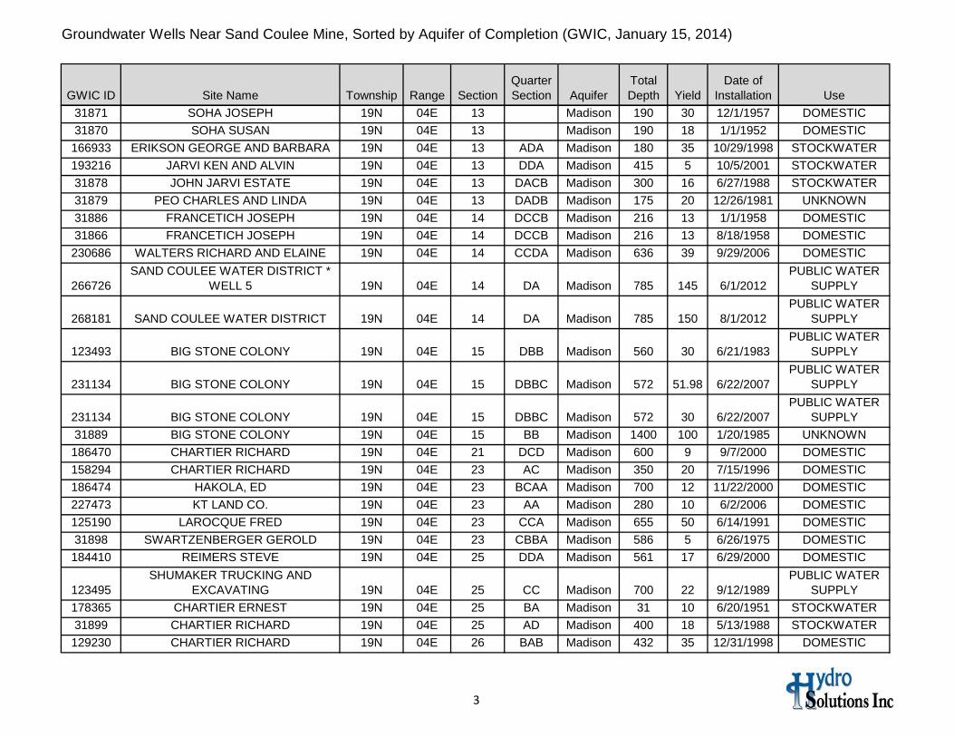
Groundwater Wells Near Sand Coulee Mine, Sorted by Aquifer of Completion (GWIC, January 15, 2014)
3
GWIC ID Site Name Township Range SectionQuarter Section Aquifer
Total Depth Yield
Date of Installation Use
31871 SOHA JOSEPH 19N 04E 13 Madison 190 30 12/1/1957 DOMESTIC31870 SOHA SUSAN 19N 04E 13 Madison 190 18 1/1/1952 DOMESTIC166933 ERIKSON GEORGE AND BARBARA 19N 04E 13 ADA Madison 180 35 10/29/1998 STOCKWATER193216 JARVI KEN AND ALVIN 19N 04E 13 DDA Madison 415 5 10/5/2001 STOCKWATER31878 JOHN JARVI ESTATE 19N 04E 13 DACB Madison 300 16 6/27/1988 STOCKWATER31879 PEO CHARLES AND LINDA 19N 04E 13 DADB Madison 175 20 12/26/1981 UNKNOWN31886 FRANCETICH JOSEPH 19N 04E 14 DCCB Madison 216 13 1/1/1958 DOMESTIC31866 FRANCETICH JOSEPH 19N 04E 14 DCCB Madison 216 13 8/18/1958 DOMESTIC230686 WALTERS RICHARD AND ELAINE 19N 04E 14 CCDA Madison 636 39 9/29/2006 DOMESTIC
266726SAND COULEE WATER DISTRICT *
WELL 5 19N 04E 14 DA Madison 785 145 6/1/2012PUBLIC WATER
SUPPLY
268181 SAND COULEE WATER DISTRICT 19N 04E 14 DA Madison 785 150 8/1/2012PUBLIC WATER
SUPPLY
123493 BIG STONE COLONY 19N 04E 15 DBB Madison 560 30 6/21/1983PUBLIC WATER
SUPPLY
231134 BIG STONE COLONY 19N 04E 15 DBBC Madison 572 51.98 6/22/2007PUBLIC WATER
SUPPLY
231134 BIG STONE COLONY 19N 04E 15 DBBC Madison 572 30 6/22/2007PUBLIC WATER
SUPPLY31889 BIG STONE COLONY 19N 04E 15 BB Madison 1400 100 1/20/1985 UNKNOWN186470 CHARTIER RICHARD 19N 04E 21 DCD Madison 600 9 9/7/2000 DOMESTIC158294 CHARTIER RICHARD 19N 04E 23 AC Madison 350 20 7/15/1996 DOMESTIC186474 HAKOLA, ED 19N 04E 23 BCAA Madison 700 12 11/22/2000 DOMESTIC227473 KT LAND CO. 19N 04E 23 AA Madison 280 10 6/2/2006 DOMESTIC125190 LAROCQUE FRED 19N 04E 23 CCA Madison 655 50 6/14/1991 DOMESTIC31898 SWARTZENBERGER GEROLD 19N 04E 23 CBBA Madison 586 5 6/26/1975 DOMESTIC184410 REIMERS STEVE 19N 04E 25 DDA Madison 561 17 6/29/2000 DOMESTIC
123495SHUMAKER TRUCKING AND
EXCAVATING 19N 04E 25 CC Madison 700 22 9/12/1989PUBLIC WATER
SUPPLY178365 CHARTIER ERNEST 19N 04E 25 BA Madison 31 10 6/20/1951 STOCKWATER31899 CHARTIER RICHARD 19N 04E 25 AD Madison 400 18 5/13/1988 STOCKWATER129230 CHARTIER RICHARD 19N 04E 26 BAB Madison 432 35 12/31/1998 DOMESTIC

Groundwater Wells Near Sand Coulee Mine, Sorted by Aquifer of Completion (GWIC, January 15, 2014)
4
GWIC ID Site Name Township Range SectionQuarter Section Aquifer
Total Depth Yield
Date of Installation Use
205577 ROBERTSON BOB 19N 04E 28 ACA Madison 740 50 6/13/2003 DOMESTIC139022 KONESKY GEORGE AND DIANE 19N 04E 28 CBB Madison 675 25 4/20/1993 STOCKWATER
2253ASHMORE JOHN * BOX 47 SAND
COULEE MT 19N 04E 13 CCBC Morrison 85 DOMESTIC2272 SWARTZENBURGER GERALD 19N 04E 23 CBBA Morrison 248 3 11/12/1973 DOMESTIC2265 MBMG RESEARCH WELL * C7-47 19N 04E 23 ACDA Morrison 47 RESEARCH
146929 MBMG RESEARCH WELL * C-5 19N 04E 23 CADA Morrison 75 2/22/1984 RESEARCH146892 MBMG RESEARCH WELL * C-9 19N 04E 23 ADCD Morrison 172.5 RESEARCH
2279CHARTIER RANCH * MBMG
RESEARCH WELL C-10 19N 04E 26 AABB Morrison 110 RESEARCH193218 DIAMOND LAZY A INC 19N 04E 27 CC Morrison 440 15 10/23/2001 STOCKWATER
Morrison Formation

Appendix B
File Geodatabase
Appendix C
Horizontal Well Model Calculations

Horizontal Well Model Calculations Completed: April 24, 2014
Section 1. Horizontal Well Discharge Using H Well Model and Dupuit-Forchheimer Model 1.A Calculations of Horizontal Well Discharge Using the H Well Model for Two Well Diameters
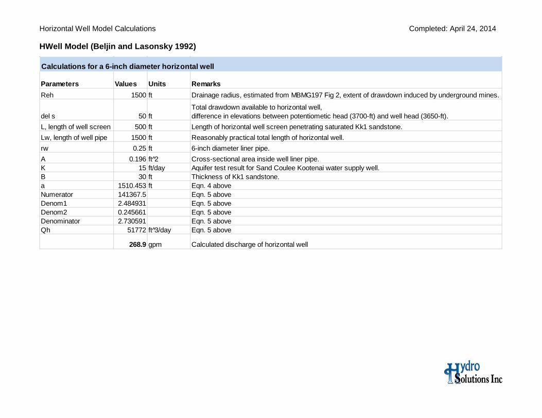
Horizontal Well Model Calculations Completed: April 24, 2014 HWell Model (Beljin and Lasonsky 1992)
Calculations for a 6-inch diameter horizontal well
Parameters Values Units RemarksReh 1500 ft Drainage radius, estimated from MBMG197 Fig 2, extent of drawdown induced by underground mines.
del s 50 ftTotal drawdown available to horizontal well, difference in elevations between potentiometic head (3700-ft) and well head (3650-ft).
L, length of well screen 500 ft Length of horizontal well screen penetrating saturated Kk1 sandstone.Lw, length of well pipe 1500 ft Reasonably practical total length of horizontal well.rw 0.25 ft 6-inch diameter liner pipe.A 0.196 ft 2̂ Cross-sectional area inside well liner pipe.K 15 ft/day Aquifer test result for Sand Coulee Kootenai water supply well.B 30 ft Thickness of Kk1 sandstone.a 1510.453 ft Eqn. 4 aboveNumerator 141367.5 Eqn. 5 aboveDenom1 2.484931 Eqn. 5 aboveDenom2 0.245661 Eqn. 5 aboveDenominator 2.730591 Eqn. 5 aboveQh 51772 ft 3̂/day Eqn. 5 above
268.9 gpm Calculated discharge of horizontal well

Horizontal Well Model Calculations Completed: April 24, 2014 HWell Model (Beljin and Lasonsky 1992)
Calculations for a 4-inch diameter horizontal well
Parameters Values Units RemarksReh 1500 ft Drainage radius, estimated from MBMG197 Fig 2, extent of drawdown induced by underground mines.
del s 50 ftTotal drawdown available to horizontal well, difference in elevations between potentiometic head (3700-ft) and well head (3650-ft).
L, length of well screen 500 ft Length of horizontal well screen penetrating saturated Kk1 sandstone.Lw, length of well pipe 1500 ft Reasonably practical total length of horizontal well.rw 0.167 ft 4-inch diameter pipe.A 0.087 ft 2̂ Cross-sectional area inside well liner pipe.K 15 ft/day Aquifer test result for Sand Coulee Kootenai water supply well.B 30 ft Thickness of Kk1 sandstone.a 1510.453 ft Eqn. 4 aboveNumerator 141367.5 Eqn. 5 aboveDenom1 2.484931 Eqn. 5 aboveDenom2 0.269989 Eqn. 5 aboveDenominator 2.754919 Eqn. 5 aboveQh 51315 ft 3̂/day Eqn. 5 above
266.6 gpm Calculated discharge of horizontal well

Horizontal Well Model Calculations Completed: April 24, 2014 !.B. Calculations of Horizontal Well Discharge Using Dupuit Forchheimer Model for Two Well Diameters
Equations for Cauchy Boundary Approach
This paper give two solutions, one for a horizontal well beneath a stream, and another for a Cauchy boundary condition with the head ɸw inside the horizontal well. Solution for the Cauchy condition adapted to the Sand Coulee, Montana setting follows.

Horizontal Well Model Calculations Completed: April 24, 2014 Dupuit-Forchheimer Model (Haitjema, et al. 2010)
Calculations for a 6-inch diameter horizontal wellParameter Value Units Remarks
h 0 ft Distance of well invert above aquifer base.w 1 ft Stream width, a ficticious value which cancels out in calculation.rw 0.250 ft 6-inch diameter liner pipe.A 0.196 ft 2̂ Cross-sectional area inside well liner pipe.ɸw 0.5 ft Head inside the horizontal well pipe is at top of pipe.ɸL 50 ft The head at distance (L) from horizontal well, i.e. the head available for inflow to well (3700-3650 ft).k 15 ft/day Aquifer test result for Sand Coulee Kootenai water supply wellH 30 ft Thickness of aquiferL 1000 ft A distance (L) from the well with head ϕL.Lw 1500 ft Total length of horizontal well (used in pipe friction loss calculation if performed)σ calculated ft 2̂/day Inflow rate per unit length, calculated with Eqn. 4 above
Solution with Cauchy Boundary Approach In Cauchy approach, ϕw is redefined as the head inside the horizontal well.Denom 2 0.01309 Eqn. 6 aboveSin Denom2 0.013089 Eqn. 6 aboveDenom 1 0.01309 Eqn. 6 above2 Sin Denom1 0.026178 Eqn. 6 aboveNum2 0 Eqn. 6 aboveCos Num2 1 Eqn. 6 aboveNum1 104.7167 Eqn. 6 aboveCosh Num1 1.5E+45 Eqn. 6 aboveTerm 1 0.010611 Eqn. 6 abovec1 1.188416 Eqn. 6 above; the resistance factor due to vertical flow near horizontal well.σ 41.65 ft 2̂/day Eqn. 4 above, the horizotal well inflow per unit length.Screen length 500 ft Length of horizontal well screen.Total Well Inflow 20,826 ft^3/day
or 108 gpm Calculated discharge of horizontal well

Horizontal Well Model Calculations Completed: April 24, 2014 Dupuit-Forchheimer Model (Haitjema, et al. 2010)
Calculations for a 4-inch diameter horizontal wellParameter Value Units Remarks
h 0 ft Distance of well invert above aquifer base.w 1 ft Stream width, a ficticious value which cancels out in calculation.rw 0.167 ft 4-inch diamter well.A 0.087 ft 2̂ Cross-sectional area inside well liner pipe.ɸw 0.333 ft Head inside the horizontal well pipe is at top of pipe.ɸL 50 ft The head at distance (L) from horizontal well, i.e. the head available for inflow to well (3700-3650 ft).k 15 ft/day Aquifer test result for Sand Coulee Kootenai water supply wellH 30 ft Thickness of aquiferL 1000 ft A distance (L) from the well with head ϕL.Lw 1500 ft Total length of horizontal well (used in pipe friction loss calculation if performed)σ calculated ft 2̂/day Inflow rate per unit length, calculated with Eqn. 4 above
Solution with Cauchy Boundary Approach In Cauchy approach, ϕw is redefined as the head inside the horizontal well.Denom 2 0.008726 Eqn. 6 aboveSin Denom2 0.008726 Eqn. 6 aboveDenom 1 0.008726 Eqn. 6 above2 Sin Denom1 0.017453 Eqn. 6 aboveNum2 0 Eqn. 6 aboveCos Num2 1 Eqn. 6 aboveNum1 104.7167 Eqn. 6 aboveCosh Num1 1.5E+45 Eqn. 6 aboveTerm 1 0.010611 Eqn. 6 abovec1 1.197021 Eqn. 6 above; the resistance factor due to vertical flow near horizontal well.σ 41.49 ft 2̂/day Eqn. 4 above, the horizotal well inflow per unit length.Screen length 500 ft Length of horizontal well screen.Total Well Inflow 20,746 ft^3/dayor 108 gpm Calculated discharge of horizontal well

Horizontal Well Model Calculations Completed: April 24, 2014
Section 2. Horizontal Well Discharge Accounting for Friction Losses 2.A Calculations of Horizontal Well Discharge Using the H Well Model for Two Well Diameters With Friction Losses
Calculations for a 6-inch diameter horizontal well
Parameters Values Units RemarksReh 1500 ft Drainage radius, estimated from MBMG197 Fig 2, extent of drawdown induced by underground mines.
del S 50 ftTotal drawdown available to horizontal well, difference in elevations between potentiometic head (3700-ft) and well head (3650-ft).
Available head 41.8 ft Adjusted drawdown available to well after friction loss (below) is accounted for. Determined by iteration.L, length of well screen 500 ft Length of horizontal well screen penetrating saturated Kk1 sandstone.Lw, length of well pipe 1500 ft Reasonably practical total length of horizontal well.rw 0.25 ft 6-inch diameter liner pipe.A 0.196344 ft 2̂ Cross-sectional area inside well liner pipe.K 15 ft/day Aquifer test result for Sand Coulee Kootenai water supply well.B 30 ft Thickness of Kk1 sandstone.a 1510.453 ft Eqn. 4 aboveNumerator 118183.2 Eqn. 5 aboveDenom1 2.484931 Eqn. 5 aboveDenom2 0.245661 Eqn. 5 aboveDenominator 2.730591 Eqn. 5 aboveQh 43281 ft 3̂/day Eqn. 5 above
224.8 gpm Calculated discharge of horizontal wellv 2.551 ft/sec Velocity of discharge in liner pipe of diameter rw.
Friction Loss Friction losses in pipe reduce the total head available to drive gravity flow.vk (kinematic viscosity) 1.67E-05 ft 2̂/sec Water at 40F.Nr = DV/vk 7.64E+04 unitless Reynolds Number.e/D 0.00100 unitless Using e-value for galvanized iron pipe.f (friction factor) 0.027 unitless From Moody diagram.hl (head loss) 8.19 ft Friction loss. Subtract this from del s to give Available head.Total head loss 49.99 ft Value should approach but not exceed Available head.

Horizontal Well Model Calculations Completed: April 24, 2014
Calculations for a 4-inch diameter horizontal wellParameters Values Units RemarksReh 1500 ft Drainage radius, estimated from MBMG197 Fig 2, extent of drawdown induced by underground mines.
del S 50 ftTotal drawdown available to horizontal well, difference in elevations between potentiometic head (3700-ft) and well head (3650-ft).
Available head 25.80 ft Adjusted drawdown available to well after friction loss (below) is accounted for. Determined by iteration.L, length of well screen 500 ft Length of horizontal well screen penetrating saturated Kk1 sandstone.Lw, length of well pipe 1500 ft Reasonably practical total length of horizontal well.rw 0.167 ft 6-inch diameter liner pipe.A 0.087 ft 2̂ Cross-sectional area inside well liner pipe.K 15 ft/day Aquifer test result for Sand Coulee Kootenai water supply well.B 30 ft Thickness of Kk1 sandstone.a 1510.453 ft Eqn. 4 aboveNumerator 72945.63 Eqn. 5 aboveDenom1 2.484931 Eqn. 5 aboveDenom2 0.269989 Eqn. 5 aboveDenominator 2.754919 Eqn. 5 aboveQh 26478 ft 3̂/day Eqn. 5 above
137.5 gpm Calculated discharge of horizontal wellv 3.512 ft/sec Velocity of discharge in liner pipe of diameter rw.Friction Loss Friction losses in pipe reduce the total head available to drive gravity flow.vk (kinematic viscosity) 1.67E-05 ft 2̂/sec Water at 40F.Nr = DV/vk 7.01E+04 unitless Reynolds Number.e/D 0.00150 unitless Using e-value for galvanized iron pipe.f (friction factor) 0.028 unitless From Moody diagram.hl (head loss) 24.13 ft Friction loss. Subtract this from del s to give Available head.Total head loss 49.93 ft Value should approach but not exceed Available head.

Horizontal Well Model Calculations Completed: April 24, 2014 2.B Calculations of Horizontal Well Discharge Using the Dupuit-Forchheimer Model for Two Well Diameters With Friction Losses
Calculations for a 6-inch diameter horizontal wellParameter Value Units Remarks
h 0 ft Distance of well invert above aquifer base.w 1 ft Stream width, a ficticious value which cancels out in calculation.rw 0.25 ft 6-inch diameter liner pipe.A 0.196 ft 2̂ Head inside the horizontal well pipe is at top of pipe.ɸw 0.5 ft Head inside the horizontal well pipe.ɸL 50 ft The head at distance (L) from horizontal well, i.e. the head available for inflow to well (3700-3650 ft).
Available Head 48 ft Adjusted head available to well after friction loss (below) is accounted for. Determined by iteration.k 15 ft/day Aquifer test result for Sand Coulee Kootenai water supply wellH 30 ft Thickness of aquiferL 1000 ft A distance (L) from the well with head ϕL.Lw 1500 ft Total length of horizontal well (used in pipe friction loss calculation if performed)σ calculated ft 2̂/day Inflow rate per unit length, calculated with Eqn. 4 above
Solution with Cauchy Boundary Approach In Cauchy approach, ϕw is redefined as the head inside the horizontal well.Denom 2 0.01309 Eqn. 6 aboveSin Denom2 0.013089 Eqn. 6 aboveDenom 1 0.01309 Eqn. 6 above2 Sin Denom1 0.026178 Eqn. 6 aboveNum2 0 Eqn. 6 aboveCos Num2 1 Eqn. 6 aboveNum1 104.7167 Eqn. 6 aboveCosh Num1 1.5E+45 Eqn. 6 aboveTerm 1 0.010611 Eqn. 6 abovec1 1.188416 Eqn. 6 above; the resistance factor due to vertical flow near horizontal well.σ 39.97 ft 2̂/day Eqn. 4 above, the horizotal well inflow per unit length.Screen length 500 ft Length of horizontal well screen.Total Well Inflow 19,985 ft^3/day
or 104 gpm Calculated discharge of horizontal wellv 1.178 ft/sec Velocity of discharge in liner pipe of diameter rw.
Friction Loss: Friction losses in pipe reduce the total head available to drive gravity flow.vk (kinematic viscosity) 1.67E-05 ft 2̂/sec Water at 40F.Nr = DV/vk 3.53E+04 unitless Reynolds Number.e/D 0.0010 unitless Using e-value for galvanized iron pipe.f (friction factor) 0.027 unitless From Moody diagram.hl (head loss) 1.75 ft Friction loss. Subtract this from potentiometric head (ɸL) to give Available head.Total head loss 49.75 ft Value should approach but not exceed Available head.

Horizontal Well Model Calculations Completed: April 24, 2014
Calculations for a 4-inch diameter horizontal wellParameter Value Units Remarks
h 0 ft Distance of well invert above aquifer base.w 1 ft Stream width, a ficticious value which cancels out in calculation.rw 0.167 ft 4-inch diameter liner pipe.A 0.087 ft 2̂ Cross-sectional area inside well liner pipe.ɸw 0.333 ft Head inside the horizontal well pipe is at top of pipe.ɸL 50 ft The head at distance (L) from horizontal well, i.e. the head available for inflow to well (3700-3650 ft).Available Head 40 ft Adjusted head available to well after friction loss (below) is accounted for. Determined by iteration.k 15 ft/day Aquifer test result for Sand Coulee Kootenai water supply wellH 30 ft Thickness of aquiferL 1000 ft A distance (L) from the well with head ϕL.Lw 1500 ft Total length of horizontal well (used in pipe friction loss calculation if performed)σ calculated ft 2̂/day Inflow rate per unit length, calculated with Eqn. 4 above
Solution with Cauchy Boundary Approach In Cauchy approach, ϕw is redefined as the head inside the horizontal well.Denom 2 0.008726 Eqn. 6 aboveSin Denom2 0.008726 Eqn. 6 aboveDenom 1 0.008726 Eqn. 6 above2 Sin Denom1 0.017453 Eqn. 6 aboveNum2 0 Eqn. 6 aboveCos Num2 1 Eqn. 6 aboveNum1 104.7167 Eqn. 6 aboveCosh Num1 1.5E+45 Eqn. 6 aboveTerm 1 0.010611 Eqn. 6 abovec1 1.197021 Eqn. 6 above; the resistance factor due to vertical flow near horizontal well.σ 33.14 ft 2̂/day Eqn. 4 above, the horizotal well inflow per unit length.Screen length 500 ft Length of horizontal well screen.Total Well Inflow 16,569 ft^3/day 0
or 86 gpm Calculated discharge of horizontal wellv 2.198 ft/sec Velocity of discharge in liner pipe of diameter rw.
Friction Loss: Friction losses in pipe reduce the total head available to drive gravity flow.vk (kinematic viscosity) 1.67E-05 ft 2̂/sec Water at 40F.Nr = DV/vk 4.39E+04 unitless Reynolds Number.e/D 0.0015 unitless Using e-value for galvanized iron pipe.f (friction factor) 0.028 unitless From Moody diagram.hl (head loss) 9.45 ft Friction loss. Subtract this from potentiometric head (ɸL) to give Available head.Total head loss 49.45 ft Value should approach but not exceed Available head.

Appendix D
AnAqSim Model Output
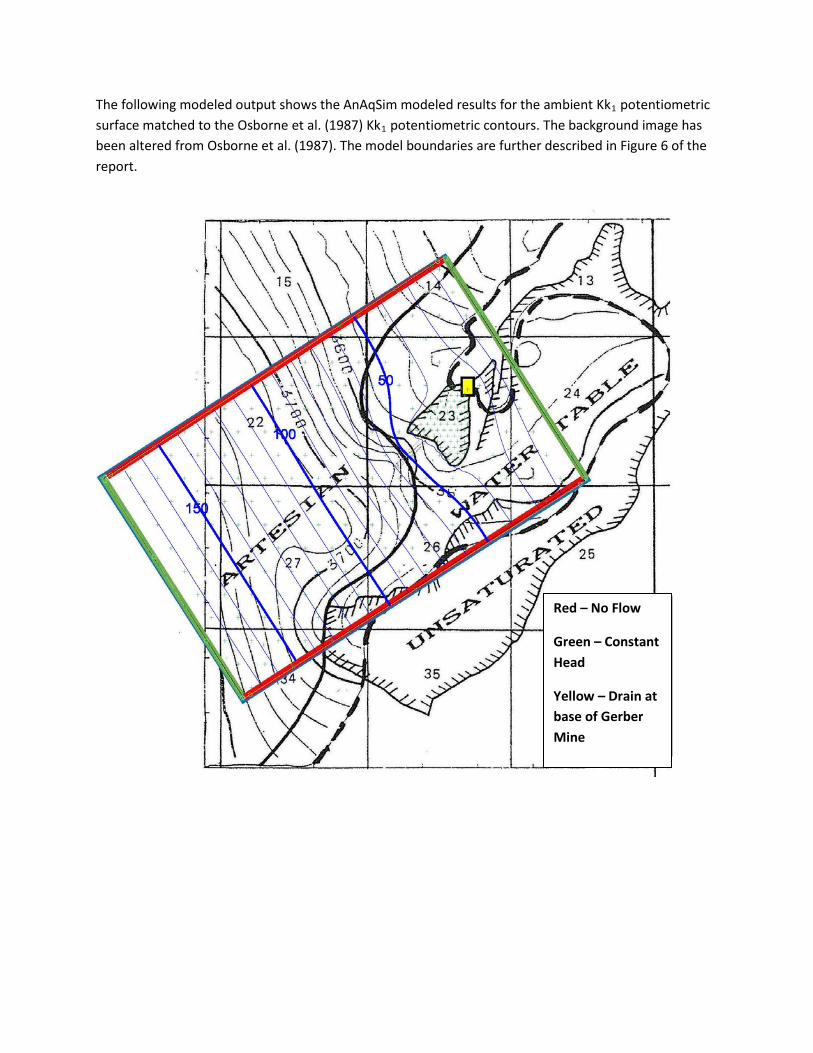
The following modeled output shows the AnAqSim modeled results for the ambient Kk1 potentiometric surface matched to the Osborne et al. (1987) Kk1 potentiometric contours. The background image has been altered from Osborne et al. (1987). The model boundaries are further described in Figure 6 of the report.
Red – No Flow
Green – Constant Head
Yellow – Drain at base of Gerber Mine

!?
50
100
150Drainage Well
25
75
125
175
Copyright:© 2013 National Geographic Society, i-cubed
Appendix DAnAqSim Steady State
Kootenai Aquifer Potentiometric Contours Showing the Effects of an
Upgradient Vertical Drainage Well0 2,500 5,000
Feet
«Prepared By: R. SvingenProduction Date: April 30, 2014Original Scale: 1:28,000File: SandCoulee_1wellModel043014.mxd
Potentiometric Contour (5ft Interval)
!?Drainage Well (Location Approximatefor Model)
Geber Mine Boundary(General Extent for Model)
Constant Head BoundaryNo Flow Boundary
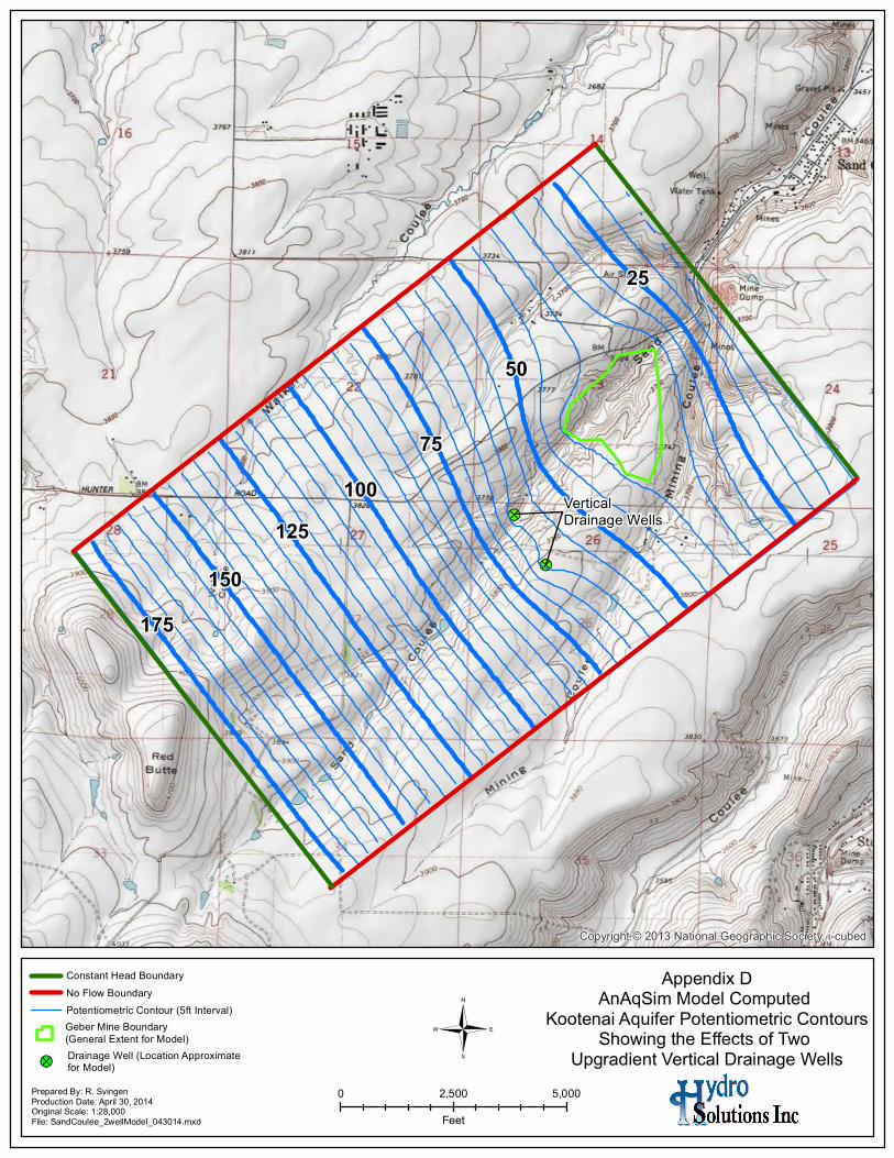
!?
!?
50
25
100
150
25
75
125
175
Copyright:© 2013 National Geographic Society, i-cubed
Appendix DAnAqSim Model Computed
Kootenai Aquifer Potentiometric ContoursShowing the Effects of Two
Upgradient Vertical Drainage Wells0 2,500 5,000
Feet
«Prepared By: R. SvingenProduction Date: April 30, 2014Original Scale: 1:28,000File: SandCoulee_2wellModel_043014.mxd
Vertical Drainage Wells
Potentiometric Contour (5ft Interval)
!?Drainage Well (Location Approximatefor Model)
Geber Mine Boundary(General Extent for Model)
Constant Head BoundaryNo Flow Boundary


![A History of Sand Coulee [INDEX] Giannini, Ruby M. … · A History of Sand Coulee [INDEX] Courtesy of Janet Thomson, ... Bishop, F.W. 50 Blending, ... Casey 86,89,96](https://img.pdfslide.us/doc/110x75/5b78ef5b7f8b9a6a498c82a9/a-history-of-sand-coulee-index-giannini-ruby-m-a-history-of-sand-coulee.jpg)