DOT HS 813 062 May 2021

Pilot Test of a Methodology for an Observation Survey of Motorcycle Personal Protective Equipment

DISCLAIMER

This publication is distributed by the U.S. Department of Transportation, National Highway Traffic Safety Administration, in the interest of information exchange. The opinions, findings, and conclusions expressed in this publication are those of the authors and not necessarily those of the Department of Transportation or the National Highway Traffic Safety Administration. The United States Government assumes no liability for its contents or use thereof. If trade names, manufacturers’ names, or specific products are mentioned, it is because they are considered essential to the object of the publication and should not be construed as an endorsement. The United States Government does not endorse products or manufacturers.

Suggested APA Format Citation: Benedick, A., De Leonardis, D., Green, J., & Petraglia, E. (2021, May). Pilot test of a methodology for an observation survey of motorcycle personal protective equipment (Report No. DOT HS 813 062). National Highway Traffic Safety Administration.

i

Technical Report Documentation Page

Form DOT F 1700.7 (8-72) Reproduction of completed page authorized

1. Report No. DOT HS 813 062

2. Government Accession No. 3. Recipient’s Catalog No.

4. Title and Subtitle Pilot Test of a Methodology for an Observation Survey of Motorcycle Personal Protective Equipment

5. Report Date May 2021

7. Authors Benedick, A., De Leonardis, D., Green, J., & Petraglia, E.

8. Performing Organization Report No.

9. Performing Organization Name and Address 10. Work Unit No. (TRAIS) Westat, Inc. 1600 Research Boulevard Rockville, MD 20850

11. Contract or Grant No DTNH22-11-D000222L/0007

12. Sponsoring Agency Name and Address National Highway Traffic Safety Administration Office of Behavioral Safety Research 1200 New Jersey Avenue SE Washington, DC 20590

13. Type of Report and Period Covered Final Report, 9/28/2016 – 12/28/2018 14. Sponsoring Agency Code

15. Supplementary Notes Kathryn Wochinger was the project manager for this study.

16. Abstract

Motorcycle personal protective equipment (PPE), an important traffic safety countermeasure, can include a safety-certified helmet, impact- and skid-resistant jackets and pants, motorcycle gloves, and sturdy, over-ankle boots. NHTSA, State highway safety offices (SHSO), and motorcycle safety groups conduct programs to encourage motorcyclists to use protective gear, especially helmets, but the impact of these programs is not well understood. Compared to observation surveys of seat belt use, observation surveys of motorcycle PPE use are not common, and the methodology for such surveys is not well established. This study sought to develop a methodology for an observation survey of motorcycle PPE that would be resource-efficient, valid, and adaptable to any jurisdiction. The design was implemented in Florida, with two rounds of data collection. The survey used a probability-based sample of road segments stratified by four State regions and road types, including roads classified as motorcycle “Best Rides.” The sample selected road segments per probability proportional to size (PPS), with the length of road segment as the measure of size. The first round resulted in 841 motorcyclists observed, with a 43% mean use rate of USDOT-certified helmets, and a standard error of 17%. The second round of data collection adjusted the sampling by using an equal probability sample of road segments, not PPS. The second-round results resulted in 873 motorcyclists observed, with a 61% mean use rate of USDOT-certified helmets, and a reduced standard error of 7.7%. The results suggest that it is crucial to oversample road segments that are likely to have higher rates of motorcycle traffic, such as the “Best Rides” stratum. In addition, oversampling arterial road segments may increase sample yields. Results also showed that selecting road segments per probability proportional to size (PPS) - when the measure of size is road segment length - was not efficient for motorcycle observations. A more efficient measure of size for motorcycle traffic is likely to be motorcycle volume at the road segment level. Otherwise, selecting road segments per equal probability, as opposed to PPS, may increase sample yield.

17. Key Words Motorcycle, safety gear, observation survey, helmet, motorcycle personal protective equipment

18. Distribution Statement The document is available to the public through the National Technical Information Service, www.ntis.gov.

19. Security Classification of this report Unclassified

20. Security Classification of this page Unclassified

21. No. of Pages

57 22. Price

ii

Acronyms ART arterials AVMT annual vehicle miles traveled CI controlled intersection CUTR Center for Urban Transportation Research CV coefficient of variation DVMT daily vehicle miles traveled FARS Fatality Analysis Reporting System FMVSS Federal Motor Vehicle Safety Standard GIS geographic information systems LAH limited access highway LCI lower confidence interval UCI upper confidence interval LOC local roads MOS measure of size MSA Metropolitan Statistical Area MT moving traffic NCSA National Center for Statistics and Analysis NOPUS National Occupant Protection Use Survey NTSS-III National Travel Speed Survey III NSUBS National Survey of the Use of Booster Seats PPE personal protective equipment PPS probability proportional to size Region region of the State RPA rural principle arterial RSE relative standard error SRS simple random sampling STE standard error TIGER Topologically Integrated Geographic Encoding and Referencing UMA urban minor arterial UPA urban principal arterial

iii

Table of Contents

Executive Summary ...................................................................................................................... v Study Purpose ........................................................................................................................... v Design Considerations and Challenges ..................................................................................... v Method ...................................................................................................................................... v

First Round of Data Collection .......................................................................................... vi Second Round of Data Collection..................................................................................... vii

Results .................................................................................................................................... viii

Introduction ................................................................................................................................... 1 Background ............................................................................................................................... 1 Study Objectives ....................................................................................................................... 1 Study Design ............................................................................................................................. 1

Round One of Data Collection ..................................................................................................... 3 Methodology ............................................................................................................................. 3

Sample Design and Scheduling .......................................................................................... 3 Data Collection ................................................................................................................. 10 Field Staff Recruitment and Hiring................................................................................... 10

Analysis................................................................................................................................... 19 Weighting .......................................................................................................................... 19 Round One Findings ......................................................................................................... 21 PPE Use ............................................................................................................................ 23

Round One Performance and Limitations............................................................................... 23

Round Two of Data Collection................................................................................................... 24 Methodology ........................................................................................................................... 24

Sample Design and Scheduling ........................................................................................ 24 Data Collection ................................................................................................................. 27

Analysis................................................................................................................................... 27 Weighting .......................................................................................................................... 27 Findings............................................................................................................................. 29

Discussion..................................................................................................................................... 39 Potential Methodology for States............................................................................................ 39

State Specific Surveys....................................................................................................... 40 Sample............................................................................................................................... 41 Data Collection ................................................................................................................. 41 Imputation, Weighting, Point and Variance Estimation ................................................... 42 National Survey of PPE Use ............................................................................................. 44

Lessons Learned...................................................................................................................... 45

References .................................................................................................................................... 46

Tables Table 1. Definitions of codes in the road segment file ................................................................... 4 Table 2. Expected allocation of road segment sample, using road segment length only ............... 6

iv

Table 3. Optimized road segment sample allocation ...................................................................... 7 Table 4. Expected Phase I road segment sample sizes ................................................................... 7 Table 5. Round One, Phase I road segment sample road type variables ........................................ 8 Table 6. Round One, Phase II actual road segment sample size by road type................................ 8 Table 7. Expected precision ............................................................................................................ 9 Table 8. Descriptive statistics for Round One moving traffic study base weights ....................... 20 Table 9. Sample design characteristics and observation sample sizes.......................................... 21 Table 10. Actual precision ............................................................................................................ 22 Table 11. Round One moving traffic survey results ..................................................................... 22 Table 12. Round One controlled intersection survey results for operators ................................... 23 Table 13. Optimized road segment sample allocation .................................................................. 25 Table 14. Expected Phase I road segment sample sizes ............................................................... 25 Table 15. Round Two Phase I road segment sample road type variables ..................................... 26 Table 16. Round Two Phase II actual road segment sample sizes by road type .......................... 26 Table 17. Expected sample design characteristics and observation sample sizes ........................ 27 Table 18. Expected precision ........................................................................................................ 27 Table 19. Round Two moving traffic survey, descriptive statistics base weights ........................ 28 Table 20. Actual sample design characteristics ............................................................................ 29 Table 21. Actual precision ............................................................................................................ 29 Table 22. Rounds One and Two moving traffic survey results on helmet use, operators and

passengers ..................................................................................................................... 30 Table 23. Rounds One and Two moving traffic survey results on helmet use, operators only .... 31 Table 24. Rounds One and Two controlled intersection survey results, operators and passengers

...................................................................................................................................... 33 Table 25. Rounds One and Two controlled intersection survey results, operators only .............. 34 Table 26. Rounds One and Two use rate of PPE besides helmets, operators only ....................... 35 Table 27. Rounds One and Two use rate of boots among operators, by motorcycle type, and

region ............................................................................................................................ 35 Table 28. Rounds One and Two use rate of gloves among operators, by motorcycle type, and

region ............................................................................................................................ 36 Table 29. Rounds One and Two use rate of jackets among operators, by motorcycle type and

region ............................................................................................................................ 36 Table 30. Rounds One and Two use rate of pants among operators, motorcycle type and region37 Table 31. Rounds One and Two helmet use rate of helmets among operators, by PPE type ....... 37 Table 32. Rounds One and Two controlled intersection survey results of use rate of PPE,

operators only ............................................................................................................... 38 Table 33. Estimate of labor hours for a State-based survey of PPE use ....................................... 43

Figures Figure 1. Training slides for classifying helmet type. .................................................................. 11 Figure 2. High-visibility gear examples........................................................................................ 12 Figure 3. Field guide on motorcycles for data collection. ............................................................ 14 Figure 4. Moving traffic data collection form. ............................................................................. 16 Figure 5. Collection form for stopped motorcycles. ..................................................................... 18

v

Executive Summary Motorcycle personal protective equipment (PPE) is an important traffic safety countermeasure for motorcyclists. Lacking the protective enclosure of a passenger vehicle, the different types of PPE, including a safety-certified helmet, impact and skid resistant jacket and pants, gloves, and sturdy over-the ankle footwear, protect the motorcyclist from flying road debris while riding, and most important, in the event of a crash. Safety gear characterized by high-visibility or retroreflective materials can also be considered a type of, or part of PPE. Motorcyclists use any combination of PPE, and sometimes none. A motorcycle helmet that meets the U.S. Department of Transportation safety standard1 is the most important element of PPE, as USDOT-certified helmets are proven to reduce head injuries and save lives. Other PPE can also mitigate injuries and save lives.

The National Highway Traffic Safety Administration, State Highway Safety Offices (SHSO), and motorcycle safety groups conduct programs to encourage the use of motorcycle PPE. These programs support NHTSA’s mission to save lives and reduce injuries, but their effectiveness is not determined, largely because data on the use of PPE are not readily available.

Study Purpose The purpose of this study was to develop a methodology for measuring the use of motorcycle PPE that would be valid, efficient, and feasible in any jurisdiction. NHTSA publishes uniform guidelines for observation surveys of seat belt use, but there are no uniform guidelines for observation surveys of motorcyclists’ use of safety gear. The present study developed and implemented an observation survey of motorcyclist PPE use, with the goal of identifying factors involved in survey efficiency and validity, and that would be adaptable to any jurisdiction.

The methodology included a sampling plan, selection of sites, hiring and training of field staff, data collection, data entry, and analysis. The design provided a probability-based estimate of PPE use among motorcyclists. The approach incorporated considerations used in NHTSA’s Uniform Criteria for State Observational Surveys of Seat Belt Use (23 CFR, Part 1340), to define the sampling frame and target population exclusions (see also NHTSA, 2000).

Design Considerations and Challenges The population of inference was all motorcyclists2 (operators and passengers) riding on public roadways in Florida. The target population, which in survey design reflects practical restrictions and in this way, differs from the population of inference, was restricted to motorcyclists riding during daylight hours, due to the challenges of making reliable nighttime observations.

Method The target population was all motorcyclists (operators and passengers) riding on public roadways in Florida during daylight hours. Florida was selected as the pilot State because it does not have a universal helmet law (resulting in a variable helmet use rate), is geographically large, with over 500,000 registered motorcycles. In addition, a substantial percentage of motorcyclists killed in

1 Federal Motor Vehicle Safety Standard (FMVSS) 218, Motorcycle helmets. 2 The motorcycle rider is the person operating the motorcycle; the passenger is a person seated on, but not operating,

the motorcycle; the motorcyclist is a general term referring to either the rider or passenger.

vi

traffic crashes in Florida were unhelmeted. Of note as well is Florida’s long riding season, which allowed for greater flexibility in scheduling data collection.

In general, the survey design followed considerations used in meeting precision requirements in NHTSA’s Uniform Criteria for State Observational Surveys of Seat Belt Use, including the following: identifying population of inference; sampling frame and target population exclusions; sample allocation and optimization; and the expected road segment and observation sample sizes and precision (23 CFR Part 1340 and NHTSA, 2000). The design also employed a Fatality Analysis Reporting System (FARS)3 criterion, which pointed to the inclusion of 27 counties that had accounted for at least 85% of FARS motorcycle fatalities across a 5-year4 period from 2011 to 2015. To increase efficiency in data collection, the counties were grouped into four regions, based on their geographic distribution.

The U.S. Census Bureau’s Topologically Integrated Geographic Encoding and Referencing, called “TIGER” data, were used as the primary source of the road segment sampling frame. The road type included three levels: limited access highways (LAH), arterials (ART), and (non-rural) local roads (LOC). Sampling exclusion rules were applied to improve the efficiency of the observation period (sample yield) by allocating sample locations to places expected to have higher yields of motorcycles. For example, rural local roads, as defined by criteria in the Census Bureau’s Metropolitan Statistical Area, were excluded, as were non-public roads, unnamed roads, unpaved roads, vehicular trails, access ramps, cul-de-sacs, traffic circles, and service drives.

In addition, the sample included a “Best Rides” stratum consisting of road segments that coincided with popular motorcycle routes. Prior to sample selection, the road segments were stratified by into two levels (Best Rides, and all other road types combined) and sorted in the following order: by region, county, detailed road type, and a geo-spatial sort.

There were two rounds of data collection. Round One was conducted in May 2017 and Round Two was conducted in May 2018. The road segments were stratified by road type into four levels (“Best Rides,” LAH, ART, LOC) and sorted by region, county, detailed road type, and a spatial sort such that adjacent road segments on the same road were sequential in the list frame. In Round One, road segments were selected per probability proportional to size, where the measure of size was a function of road segment length. For Round Two, road segments were selected per equal probability (not PPS).

First Round of Data Collection Data were collected from 288 selected road segments, on both weekdays and weekends throughout daylight hours when visibility was best. This included rush hour and non-rush hour time periods. Weekday rush hours are defined as 7 a.m. to 9:30 a.m. and 3:30 p.m. to 6 p.m., while weekday non-rush hours comprise all other weekday data collection hours (9:30 a.m. to 3:30 p.m.). All weekend times are considered non-rush hours.

3 The Fatality Analysis Reporting System (FARS) is a nationwide census of fatal injuries suffered in motor vehicle

traffic crashes (NHTSA, 2014). See NHTSA’s brochure on FARS at https://crashstats.nhtsa.dot.gov/Api /Public/ViewPublication/811992).

4 A 5-year period is used to smooth out the year-to-year variation in the numbers of this relatively rare event.

vii

At each site, data collectors observed motorcyclist PPE use for both moving motorcyclists and stopped motorcyclists. Observing stopped motorcycles enabled data collectors to record more details related to PPE other than DOT-compliant helmet use, including the use of gloves, boots, riding pants and jacket, and high-visibility characteristics. High-visibility gear is defined in this report as clothing or equipment with highly reflective properties or colors that can be easily distinguished from any background. The fabric must be bright colors, typically fluorescent or neon yellow, green, or orange. High-visibility gear may also have retroreflective stripes or piping which make the rider more visible to other road users. In addition, traffic counts were completed at all sites as a means for obtaining roadway volume data needed to estimate weights and PPE use. Data were cleaned and weighted to allow for unbiased estimation.

Round One captured 741 motorcycle observations and 841 motorcyclists (operators and passengers combined) observations. The road segments which yielded the highest number of observations were the “Best Rides” and the arterials. Overall, the DOT-compliant helmet use rate was estimated to be 43.03% among all motorcyclists and 44.79% among operators. The 95% confidence interval was 15.02% to 76.34%. The correlation between operator and passenger DOT-compliant helmet use was 94.66% in Round One, indicating a helmeted operator was likely to have a helmeted passenger; similarly, an unhelmeted operator was likely to have an unhelmeted passenger. PPE use rates for other types of safety gear were low for operators; protective boots were observed most frequently (worn by 7.17% of operators), followed by gloves (worn by 6.34% of operators) and by armored jackets and pants (worn in 1% of operators).

Round One results indicated the sample design and study protocol, in terms of the stratification by region, road type (“Best Rides” and all other roads combined) were largely successful in meeting survey goals with respect to the total number of observations, and number of observations by road type). However, results also revealed a large variation in the standard error, which was addressed in Round Two.

Second Round of Data Collection The methodology for Round Two included design factors from Round One that were deemed effective; these factors included the stratification by region and road types (consisting of “Best Rides” and all other road types combined), but with adjustments to the way road segments were selected. Road segments in Round Two were selected with an equal probability within stratum, to increase the precision of the measures, whereas in Round One, segments were selected per PPS.

Round Two resulted in 773 motorcycles observed, 873 motorcyclists (operators and passengers combined) observed, and a mean helmet use rate of 60.90% with a confidence interval of 44.8% to 74.9%. The change in design did not negatively affect the yield, and DOT-compliant helmet use rate was observed to be 60.90% among all motorcyclists, and 60.55% among all operators. The correlation between operators and passenger DOT-compliant helmet use was 92.27%. The adjustment to the sampling approach decreased the standard error compared to Round One by 10 percentage points for all motorcyclists and operators only. Although the estimated use rates appear higher for Round Two, there is no statistically significant difference between the Round One and Round Two estimates, as the uncertainty in the Round One estimate is larger.

viii

Results The results from Rounds One and Two suggest the following proposed approach for observation probability sample surveys of motorcycle PPE use. First, to record observations efficiently, it is crucial to oversample road segments likely to have higher rates of motorcycle traffic (like the “Best Rides” stratum). Second, oversampling arterial road segments helps increase yields. Probability proportional to size sample designs may not be efficient for targeting this population, unless the appropriate measures of size are available (like motorcycle volume at the road segment level), in which case equal probability within stratum design should be considered. Large increases in observations can probably only be achieved through large increases in road segment sample sizes. Third, excluding local roads from the sample locations could dramatically increase overall observation yields.

1

Introduction

Background Motorcycle personal protective equipment, also known as safety gear, is an important traffic safety countermeasure. Designed to protect a motorcyclist in a crash, and from flying road debris, PPE includes a safety-certified helmet, impact and skid-resistant jacket and pants, safety gloves, and over-the-ankle boots. Motorcyclists may use any combination of these, or none. Helmets that meet the USDOT safety standard are the most effective type of PPE, as they are proven to save lives.5 NHTSA estimates in 2017 helmets saved the lives of 1,872 motorcyclists6 and if all motorcyclists who had crashed had worn USDOT-certified helmets, 749 more lives could have been saved (National Center for Statistics and Analysis, 2019a). NHTSA, SHSOs, and motorcycle safety advocates sponsor or deploy programs to encourage motorcyclists to use PPE every ride; these efforts are particularly relevant in States that do not have universal helmet laws. However, the impact of these programs is not well understood, largely because data on the extent of PPE use are not readily available.

The goal of this study was to develop and evaluate an observation survey of motorcycle PPE would be reliable, efficient, and valid in any jurisdiction. Valuable data on PPE use from the perspective of State motorcycle safety programs would be collected in State observation surveys. This study sought to develop a survey design that would be feasible in any jurisdiction.

Study Objectives The purpose of this study was to develop and implement an observation survey to generate a probability-based estimate of PPE use by motorcyclists. The study produced a sampling plan, data collection protocol and materials, training materials for data collectors, survey data, and this report. The sampling and data collection methodology built upon data collection protocols used in other State observation surveys and from the guidelines in NHTSA’s Uniform Criteria for State Observational Surveys of Seat Belt Use.

Study Design Florida was selected to pilot the survey due to its long riding season, large population of registered motorcycles, and partial helmet law (which results in helmet use rates that likely vary across the State). For example, in 2014 there were over 500,000 registered motorcycles in Florida, and approximately 46% of the State’s motorcyclists’ fatalities were unhelmeted.

The study used two rounds of data collection, which provided the opportunity to adjust the survey design from the first to the second rounds if necessary. The results were reviewed for efficiency, validity, and feasibility in terms of the selection of sites, hiring and training of field staff, data collection, and data entry and analysis.

Data collection occurred on weekdays and weekends during daylight hours and included rush hour and non-rush hour time periods. Weekday rush hours are defined as 7 a.m. to 9:30 a.m. and

5 Motorcycle helmets sold in the United States are required to meet Federal Motor Vehicle Safety Standard 218, motorcycle helmets. 6 The rider is the person operating the motorcycle; the passenger is a person seated on, but not operating, the motorcycle; the term “motorcyclist” refers to a rider or passenger.

2

3:30 p.m. to 6 p.m. All weekend times are considered non-rush hours. Data collection occurred on surface streets and limited access highways when motorcycles were in motion or were stopped at controlled intersections, either by a stop sign or stop light. There were two protocols for data collection, one for the moving motorcycles on LAH, and one for the stopped motorcycles at intersections. At each site, data were first collected by observing moving traffic, followed by a traffic count, and then observations of stopped traffic at controlled intersections. Observations were only made of motorcycles and motorcyclists (which includes drivers, who operate the motorcycle, and passengers), whereas all vehicles (cars, truck, motorcycles, and others) were counted during the traffic count. The function of the traffic count was to provide roadway volume data for weighting and estimating purposes. Survey methodology is discussed in more detail in the sections below.

In each region, all sites were mapped and clustered geographically. Regions were defined as groups of counties that were in close geographic proximity to each other. Clusters of sites were randomly assigned to days of the week with each cluster representing one day of work. Within a cluster, sites were assigned to a data collection day in the same random manner to represent both weekday and weekend travel. The last step involved randomly choosing the start time for the sites on the assigned day of data collection.

The data collectors used paper forms to record observational data. Given this observation survey is in its infancy and there was likely to be several revisions to the data collection instrument, it was more efficient and cost effective to develop and revise paper instruments. Additionally, it may be more economical for States to reproduce paper forms than it would be to develop electronic data collection methods, such as computer tablets.

Data were collected by pairs of data collectors, with one serving as a spotter and the other as the data recorder. All field staff attended a 2-day training session that provided an overview of the survey methodology and training on data collection protocol; scheduling and rescheduling sites; identifying site locations; completing the data collection form; submitting collected data; safety and security procedures; administrative and timekeeping procedures; quality assurance procedures; and field practice.

Data collectors were trained to identify and record DOT-compliant and novelty helmets, to identify and record the presence of other PPE, and to indicate whether the riders were using high-visibility gear. All data collectors were required to take a quiz to ensure they understood the survey terminology, protocol, and reporting requirements.

Since the observational data of PPE use were obtained from a probability sample, data weighting was required for unbiased estimation. The weights reflected the overall probability of selection, variabilities in the probabilities of selection, adjustments for imputation and nonresponse, and adjustments to population or frame totals. Estimates of PPE use for each round of data collection were created by applying the final adjusted full sample weight to the relevant study variables. The complete study design and methodology are discussed in the following chapter.

3

Round One of Data Collection

Methodology The following sections describe the sampling plan and data collection protocol. The sampling plan and methodology followed similar considerations used for determining the precision requirement in NHTSA’s Uniform Criteria for State Observational Surveys of Seat Belt Use. These considerations were applied to the sample design characteristics: the population of inference; sampling frame and target population exclusions; sample allocation and optimization; and the expected road segment and observation sample sizes and precision.

Sample Design and Scheduling Round One of the pilot study used a stratified, single stage, two-phase probability sample of road segments. Road segments are the only stage of selection, and were selected within regions. The division of the sample into regions was useful for managing and assigning the data collection workload. However, region is not itself a stage of selection. The two phases refer to the review of road segments for study eligibility and reclassification of road type, if necessary, for sample selection. The road segments were selected with PPS, where the MOS was a function of road segment length. The planned sample size included 288 road segments in 27 counties, and for a yield of approximately 592 observations (i.e., motorcycles observed). The total number of motorcyclists observed was expected to be slightly higher, since some motorcycles will have both an operator and a passenger.

Population of Inference and Target Population The population of inference is all motorcyclists (operators and passengers) riding on public roadways in Florida. A motorcycle was defined as an on-road, two- or three-wheeled motor vehicle designed to transport one or two people, including scooters, minibikes and mopeds. The target population observed was restricted to motorcyclists riding during daylight hours. Public roadways were defined as all LAH, ART and LOC in Florida, subject to the target population exclusions listed in the section below.

Sampling Frame and Target Population Exclusions Like the protocols for NHTSA’s NOPUS, national roadside surveys, and State observation motorcycle surveys, all motorcycles traveling on a selected road segment during an assigned observation period were observed. While some States may have alternative road databases, with more detailed road type classifications, the goal of this work was to develop a plan that would be accessible to all States, not just those with specialized frames. As such, the U.S. Census Bureau’s TIGER data were the primary source of the road segment sampling frame, subject to some exclusions, discussed below.

TIGER road segments are classified by the U.S .Census Bureau using the Master Address File and TIGER. Using the MAF/TIGER Feature Classification Code (MTFCC), there are three major road type classifications: (1) Primary Roads (or Limited Access Highway), (2) Secondary Roads (or Arterials), and (3) Local Roads. Table 1 shows the codes and definitions for the road segments used in the sampling plan.

4

Table 1. Definitions of codes in the road segment file

Code Name Definition

S1100 Primary Road /LAH

Primary roads are generally divided, limited-access highways within the interstate highway system or under State management, and are distinguished by the presence of interchanges. These highways are accessible by ramps and may include some toll highways.

S1200 Secondary Road/ART

Secondary roads are main arteries, usually in the U.S. Highway, State Highway, or County Highway system. These roads have one or more lanes of traffic in each direction, may or may not be divided, and usually have at-grade intersections with many other roads and driveways, and often have both a local name and a route number.

S1400 Local Neighborhood Road, Rural Road, City Street/LOC

Generally, these are paved non-arterial streets, roads, or byways that usually have a single lane of traffic in each direction. They may be privately or publicly maintained. Scenic park roads would be included, as would (depending on the region of the country) some unpaved roads.

The final road segment sampling frame included all eligible TIGER road segments, after applying the following exclusion criteria:

• Restricting the target population to a subset of counties that account for at least 85% of FARS motorcycle fatalities within the State across a 5-year7 period (2011 to 2015). This exclusion improves the efficiency of observations. It involved the rank ordering of the counties in descending order of fatalities, and selecting the top counties that summed to more than 85% resulted in an initial list of 25 of Florida’s 67 counties. As allowed per the Final Rule for NHTSA’s Uniform Criteria for State Observational Surveys of Seat Belt Use, Marion County was exchanged for Okaloosa, Santa Rosa, and Walton counties, to maintain the ≥ 85% threshold and create four distinct regions for data collection within the State. Four distinct regions were preferable from an operations point of view. The result was a final list of 27 counties.

• Excluding rural local roads in non-MSA counties,8 based on the Census Bureau’s July 2015 MSA definitions. This exclusion also makes the required observation study more efficient, by allocating the sample in places with higher expected yields.

• Excluding non-public roads, unnamed roads, unpaved roads, vehicular trails, access ramps, cul-de-sacs, traffic circles, and service drives. This exclusion limits observations to motorcycles on public roads and routine passenger vehicle traffic.

The exclusions described above are identical to those permitted under NHTSA’s Final Rule for the Uniform Criteria for State Observational Surveys of Seat Belt Use.

The TIGER road segment sample was then overlaid with a list of Florida’s popular motorcycle riding routes9 using Geographic Information System coordinates. Road segments appearing on the popular riding routes list were flagged for oversampling. Road segments otherwise subject to

7 A 5-year period is used to smooth out the year-to-year variation in the numbers of this relatively rare event. 8 See www.census.gov/geographies/reference-files/time-series/demo/metro-micro/delineation-files.html. 9 www.motorcycleroads.com/Routes/Florida_85.html, www.openroadjourney.com/rides-and-roads/florida, and

www.motorcycleroads.us/states/fl.html.

5

the road segment level exclusions listed above were nonetheless included if they appeared on popular riding lists.

Cost and Precision To plan for reasonable cost and precision of sampling, prior survey data were used to inform sample size calculations including estimates of helmet use rate and the expected incidence of motorcycles in the flow of motor vehicle traffic. A 2013 observation survey of motorcycle helmet use in Florida found an overall use rate of 51% (no standard error or confidence intervals were provided) (Lett, Lin, & Schultz, 2013). The 2013 survey used 12 observation sites, with observation periods one hour long, in the “top 10” highest motorcycle fatality “hotspots” counties, based on FARS data, plus two additional counties for historical comparison. A total of 486 observation sites were selected with ArcInfo types, urban principal arterial, urban minor arterial, or rural principle arterial(UPA, UMA, and RPA), all of which appear to align with the TIGER road classification of S1200/arterials, with 1-hour-long observation periods. Observation days were on Friday, Saturday, and Sunday. Total observations were of 8,404 operators and 1,271 passengers. The 2013 Florida study is a relevant resource for making sample design assumptions, such as overall helmet use rates, but given the time that has elapsed since 2013, and differences in the survey coverage of geographic area, road types, and days of week observed, comparisons between the 2013 Florida study and either round of this pilot study must be considered with caution. Based on the 2013 survey results, the present study assumed a State helmet use rate of 50%.

The rate of flow of motorcycles was another key unknown in planning a sample size necessary for reasonable precision; it is important but difficult to estimate, given the relative rarity of motorcycles in traffic. While the 2013 survey was limited to Fridays, Saturdays and Sundays, when motorcycle traffic was expected to be higher,10 the methodology for the present study did not limit data collection by the day of week, so it sought a different rate estimate for planning purposes.

A rough estimate of the rate of flow of motorcycles for this study was based instead on National NOPUS data, pooling the 2014 and 2015 Moving Traffic study data. In 2014 the NOPUS observed 684 motorcycles at 1,581 eligible sites, and in 2015 NOPUS observed 851 motorcycles at 1,901 sites, meaning that approximately 0.44 motorcycles were observed at each site (Pickrell & Li, 2016). Multiplying the rate of flow from the 2013 Florida report (0.288 motorcycles per minute) by the planned 40-minute observation period11 for the present study, implies 11.5 motorcycles per site, which is much higher. Because the design did not restrict data collection sites to higher-volume days of the week or selected road types only, the true yield per site is likely to be closer to the NOPUS-based estimate, than to the 2013 survey report-based estimate. However, by tailoring the sample design to maximize yield, the present study could improve on the NOPUS-based estimate, resulting in an expected average yield per site of 2.055 motorcycles.

Stratification and Stages of Selection The FARS criterion pointed to inclusion of 27 Florida counties; given their geographic distribution, it was operationally efficient to group the 27 counties into the four regions, and

10 The rate of flow in this instance and from the report is 0.288 motorcycles per minute. 11 A 40-minute period was selected as sufficient time for observing without incurring observer fatigue.

6

assign one data collection team (consisting of two team members) to each region. Since the included counties within each region were geographically close, it was decided that the sampling of counties within region was unnecessary, and instead, a stratified, single stage sample of road segments was used. The road segments were stratified by region and road type, and selected PPS to length with specific target sample sizes by road type stratum. For Round One, prior to sample selection, the road segments were stratified by into two levels: Best Rides, and all other road types combined, and sorted by region, county, detailed road type, and a geo-spatial sort. The Best Rides stratum included all road segments that coincided via a geo-spatial overlay with popular motorcycle riding routes listed on motorcycle riding websites.

Helmet use rates, like seat belt use rates, vary by road type; therefore, stratification by road type reduces the variance of use estimates. For example, in 2019, NOPUS reported a helmet use rate of 69.3% on surface streets (local roads and arterials) versus a rate of 73.7% on limited access highways. We also have evidence from NOPUS that helmet use rates are lower for traffic moving less than 30 mph (64.1% in 2019) versus traffic moving faster than 50 mph (72.1% in 2019), roughly corresponding to differences in speed on many of the local and arterial roads sampled.

Stratification also allows us to explicitly control the number of road segments of each road type included in the sample. Because the most road segments in the population are local roads, simple random sampling or non-stratified PPS sampling would result in a sample consisting of mostly local roads. Our experience on NOPUS is that local roads tend to have lower traffic volume (and thus carry fewer motorcycles) than arterial roads or limited access highways. Stratification is an effective way to limit the number of local road sites, maximizing sample yield (and thus sample efficiency) without negatively impacting variances. The allocation of road segments to strata and optimization is described in the following section.

Road Segment MOS, Allocation, and Optimization As with most recent road segment samples selected from TIGER, the initial consideration was to use a very basic allocation: fixed 40-road segments allocated to the “Best Rides” stratum, and strictly PPS to road segment length for all other strata. See Table 2 for the expected sample distribution by road type under this allocation.

Table 2. Expected allocation of road segment sample, using road segment length only

Road type Road segment sample size

“Best Rides” 40

Limited Access Highway (LAH) 5

Arterials (ART) 22

Local Roads (LOC) 221

Total 288

As can be seen in Table 2, a large share of the total road segment sample (221/288 road segments) was assigned to local roads (Code S1400). This outcome was not acceptable from an operational or a statistical point of view, given the low expected rates of flow of motorcycles on

7

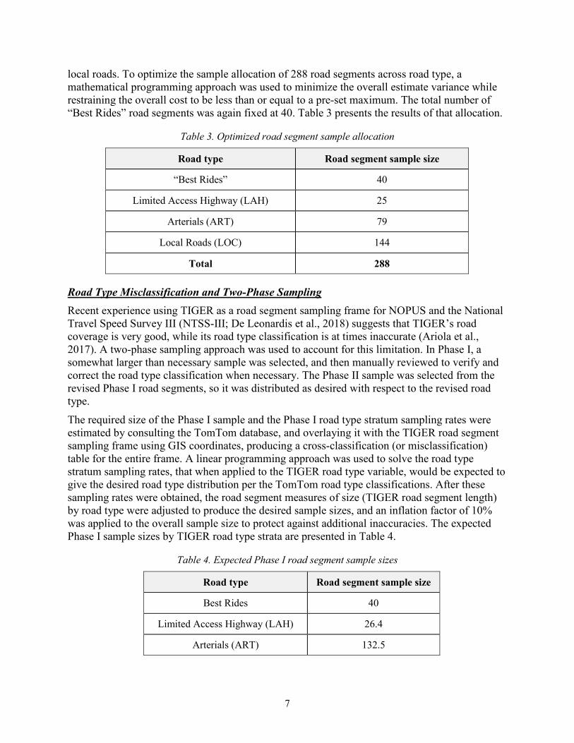
local roads. To optimize the sample allocation of 288 road segments across road type, a mathematical programming approach was used to minimize the overall estimate variance while restraining the overall cost to be less than or equal to a pre-set maximum. The total number of “Best Rides” road segments was again fixed at 40. Table 3 presents the results of that allocation.

Table 3. Optimized road segment sample allocation

Road type Road segment sample size

“Best Rides” 40

Limited Access Highway (LAH) 25

Arterials (ART) 79

Local Roads (LOC) 144

Total 288

Road Type Misclassification and Two-Phase Sampling Recent experience using TIGER as a road segment sampling frame for NOPUS and the National Travel Speed Survey III (NTSS-III; De Leonardis et al., 2018) suggests that TIGER’s road coverage is very good, while its road type classification is at times inaccurate (Ariola et al., 2017). A two-phase sampling approach was used to account for this limitation. In Phase I, a somewhat larger than necessary sample was selected, and then manually reviewed to verify and correct the road type classification when necessary. The Phase II sample was selected from the revised Phase I road segments, so it was distributed as desired with respect to the revised road type.

The required size of the Phase I sample and the Phase I road type stratum sampling rates were estimated by consulting the TomTom database, and overlaying it with the TIGER road segment sampling frame using GIS coordinates, producing a cross-classification (or misclassification) table for the entire frame. A linear programming approach was used to solve the road type stratum sampling rates, that when applied to the TIGER road type variable, would be expected to give the desired road type distribution per the TomTom road type classifications. After these sampling rates were obtained, the road segment measures of size (TIGER road segment length) by road type were adjusted to produce the desired sample sizes, and an inflation factor of 10% was applied to the overall sample size to protect against additional inaccuracies. The expected Phase I sample sizes by TIGER road type strata are presented in Table 4.

Table 4. Expected Phase I road segment sample sizes

Road type Road segment sample size

Best Rides 40

Limited Access Highway (LAH) 26.4

Arterials (ART) 132.5

8

Road type Road segment sample size

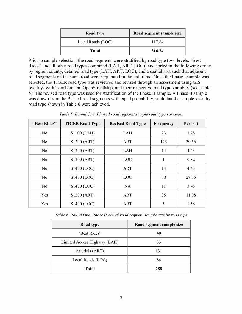
Local Roads (LOC) 117.84

Total 316.74

Prior to sample selection, the road segments were stratified by road type (two levels: “Best Rides” and all other road types combined (LAH, ART, LOC)) and sorted in the following order: by region, county, detailed road type (LAH, ART, LOC), and a spatial sort such that adjacent road segments on the same road were sequential in the list frame. Once the Phase I sample was selected, the TIGER road type was reviewed and revised through an assessment using GIS overlays with TomTom and OpenStreetMap, and their respective road type variables (see Table 5). The revised road type was used for stratification of the Phase II sample. A Phase II sample was drawn from the Phase I road segments with equal probability, such that the sample sizes by road type shown in Table 6 were achieved.

Table 5. Round One, Phase I road segment sample road type variables

“Best Rides” TIGER Road Type Revised Road Type Frequency Percent

No S1100 (LAH) LAH 23 7.28

No S1200 (ART) ART 125 39.56

No S1200 (ART) LAH 14 4.43

No S1200 (ART) LOC 1 0.32

No S1400 (LOC) ART 14 4.43

No S1400 (LOC) LOC 88 27.85

No S1400 (LOC) NA 11 3.48

Yes S1200 (ART) ART 35 11.08

Yes S1400 (LOC) ART 5 1.58

Table 6. Round One, Phase II actual road segment sample size by road type

Road type Road segment sample size

“Best Rides” 40

Limited Access Highway (LAH) 33

Arterials (ART) 131

Local Roads (LOC) 84

Total 288

9

Prior to sample selection, the road segments were stratified by road type (two levels: “Best Rides,” and all other road types (based on the Phase I improved road type) combined (LAH, ART, LOC)) and sorted by region, county, Phase I revised detailed road type (LAH, ART, LOC), and a spatial sort such that adjacent road segments on the same road were sequential in the list frame.

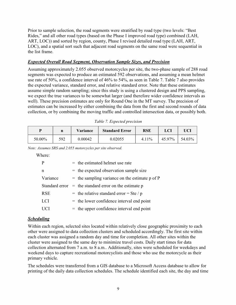
Expected Overall Road Segment, Observation Sample Sizes, and Precision Assuming approximately 2.055 observed motorcycles per site, the two-phase sample of 288 road segments was expected to produce an estimated 592 observations, and assuming a mean helmet use rate of 50%, a confidence interval of 46% to 54%, as seen in Table 7. Table 7 also provides the expected variance, standard error, and relative standard error. Note that these estimates assume simple random sampling; since this study is using a clustered design and PPS sampling, we expect the true variances to be somewhat larger (and therefore wider confidence intervals as well). These precision estimates are only for Round One in the MT survey. The precision of estimates can be increased by either combining the data from the first and second rounds of data collection, or by combining the moving traffic and controlled intersection data, or possibly both.

Table 7. Expected precision

P n Variance Standard Error RSE LCI UCI

50.00% 592 0.00042 0.02055 4.11% 45.97% 54.03%

Note: Assumes SRS and 2.055 motorcycles per site observed.

Where:

P = the estimated helmet use rate

n = the expected observation sample size

Variance = the sampling variance on the estimate p of P

Standard error = the standard error on the estimate p

RSE = the relative standard error = Ste / p

LCI = the lower confidence interval end point

UCI = the upper confidence interval end point

Scheduling Within each region, selected sites located within relatively close geographic proximity to each other were assigned to data collection clusters and scheduled accordingly. The first site within each cluster was assigned a random day and time for completion. All other sites within the cluster were assigned to the same day to minimize travel costs. Daily start times for data collection alternated from 7 a.m. to 8 a.m.. Additionally, sites were scheduled for weekdays and weekend days to capture recreational motorcyclists and those who use the motorcycle as their primary vehicle.

The schedules were transferred from a GIS database to a Microsoft Access database to allow for printing of the daily data collection schedules. The schedule identified each site, the day and time

10

of data collection, the type of study to be conducted (moving traffic or controlled intersection), the flow (direction) of traffic, the ramps to use for a limited access highway site, and the observed and intersecting roads. Data collectors were instructed to complete their observations of motorcyclists at the controlled intersection immediately after they conducted the moving traffic study and completed the traffic counts for the site. Each data collector received a schedule for their assigned sites and the quality control monitor received schedules for all 288 sites. On occasion, there was a need to reschedule data collection, in cases of bad weather, road construction, or temporary road closures. Make-up data collection was made on the same type of day (weekday or weekend) and time of day as the original assignment for the site.

In addition to the schedule, data collectors received computer-generated maps identifying the locations of all their assigned data collection sites, and the QC monitor was supplied with a complete set of maps for all four regions. The maps showed the sites by day of data collection. In addition, Google Navigation links for each site were emailed to the data collectors. Using their mobile phones or other navigation systems, data collectors could select their assigned sites on their devices, which would then link to a navigation application and provide turn-by-turn directions to the Observed Road and Intersecting Road.

Data Collection

Field Staff Recruitment and Hiring There were eight data collectors who worked in teams of two, two back-up data collectors, and one QC monitor hired. The field staff had participated successfully in previous NOPUS and NSUBS studies; and therefore, were familiar with roadside observational studies and data collection protocols.

The data collectors were screened to ensure they would be available for the training and data collection periods, had a valid driver's license, access to reliable, insured transportation, possessed the required employment qualifications, and passed an employment background screening. All candidates were required to be able to read maps and navigate to unfamiliar locations, work for up to 12 hours a day, and stand outdoors for up to 90 minutes at a time with reasonable accommodations.

Training Field staff (the data collectors, back-up data collectors, and QC monitor) were required to attend 2 full days of training in Orlando, Florida, on May 3 to 4, 2017. The training reviewed the technical and administrative protocols required to complete the data collection tasks, and each received a copy of the training manual with the training materials and briefing slides. The following topics were covered during training and in the manual:

• Overview and purpose of the survey;

• Instructions on using the maps, Google Navigation and the site schedules;

• Description of the procedures for observing motorcycles in moving traffic on surface streets and limited access highways;

• Description of the procedures for the observing stopped motorcycles at controlled intersections on surface streets and LAH ramps;

11

• Identifying the different motorcycle types and the other data collection variables;

• Completing the data collection booklet;

• Instructions for sending data to study headquarters; and

• Administrative procedures.

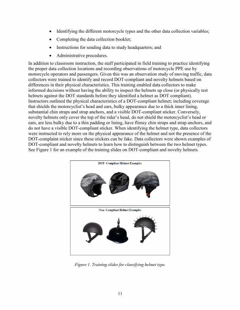
In addition to classroom instruction, the staff participated in field training to practice identifying the proper data collection locations and recording observations of motorcycle PPE use by motorcycle operators and passengers. Given this was an observation study of moving traffic, data collectors were trained to identify and record DOT-compliant and novelty helmets based on differences in their physical characteristics. This training enabled data collectors to make informed decisions without having the ability to inspect the helmets up close (or physically test helmets against the DOT standards before they identified a helmet as DOT compliant). Instructors outlined the physical characteristics of a DOT-compliant helmet; including coverage that shields the motorcyclist’s head and ears, bulky appearance due to a thick inner lining, substantial chin straps and strap anchors, and a visible DOT-compliant sticker. Conversely, novelty helmets only cover the top of the rider’s head, do not shield the motorcyclist’s head or ears, are less bulky due to a thin padding or lining, have flimsy chin straps and strap anchors, and do not have a visible DOT-compliant sticker. When identifying the helmet type, data collectors were instructed to rely more on the physical appearance of the helmet and not the presence of the DOT-complaint sticker since these stickers can be fake. Data collectors were shown examples of DOT-compliant and novelty helmets to learn how to distinguish between the two helmet types. See Figure 1 for an example of the training slides on DOT-compliant and novelty helmets.

Figure 1. Training slides for classifying helmet type.

12

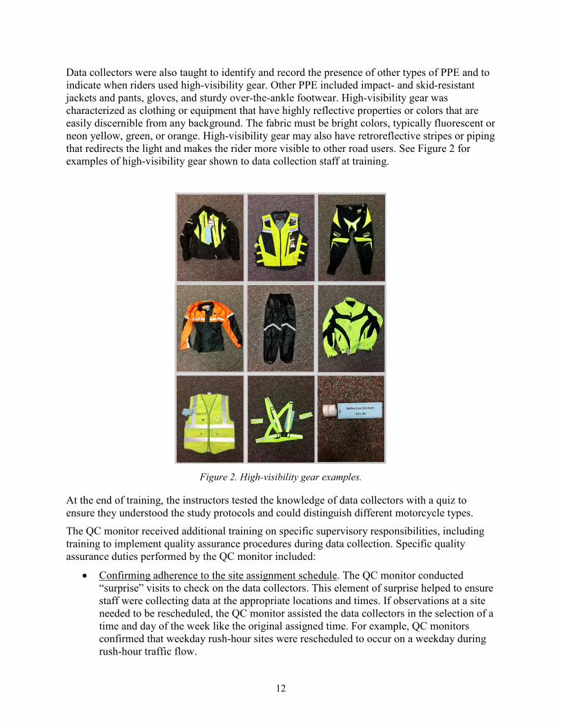
Data collectors were also taught to identify and record the presence of other types of PPE and to indicate when riders used high-visibility gear. Other PPE included impact- and skid-resistant jackets and pants, gloves, and sturdy over-the-ankle footwear. High-visibility gear was characterized as clothing or equipment that have highly reflective properties or colors that are easily discernible from any background. The fabric must be bright colors, typically fluorescent or neon yellow, green, or orange. High-visibility gear may also have retroreflective stripes or piping that redirects the light and makes the rider more visible to other road users. See Figure 2 for examples of high-visibility gear shown to data collection staff at training.

Figure 2. High-visibility gear examples.

At the end of training, the instructors tested the knowledge of data collectors with a quiz to ensure they understood the study protocols and could distinguish different motorcycle types.

The QC monitor received additional training on specific supervisory responsibilities, including training to implement quality assurance procedures during data collection. Specific quality assurance duties performed by the QC monitor included:

• Confirming adherence to the site assignment schedule. The QC monitor conducted “surprise” visits to check on the data collectors. This element of surprise helped to ensure staff were collecting data at the appropriate locations and times. If observations at a site needed to be rescheduled, the QC monitor assisted the data collectors in the selection of a time and day of the week like the original assigned time. For example, QC monitors confirmed that weekday rush-hour sites were rescheduled to occur on a weekday during rush-hour traffic flow.

13

• Monitoring compliance with the data collection procedures. During a visit to a region, the QC monitor accompanied the team through each of the data collection protocols, including: observations of moving motorcycles on surface streets and limited access highways, as well as observations of stopped motorcycles on surface streets and ramps leading from a LAH to verify that all data collection procedures were followed.

• Reporting on progress of the study. The QC monitor was vital in monitoring the overall progress of the study. Each night the QC monitors called each team to determine which sites they completed that day and the results of each site visit. The QC monitor recorded each team’s progress on a daily report form that documented the site status (complete, unable to complete, alternate site selected), total number of motorcycles observed at each site, and any comments or issues. The daily report form was emailed to the study headquarters each evening.

As an additional training resource, staff were provided with a field guide (see Figure 3) that provided key characteristics of different motorcycle types (cruiser, sport, touring, classic, scooter, moped, and other) to help the teams classify observed motorcycles.

14

Figure 3. Field guide on motorcycles for data collection.

15

Data Collection Procedures Data collection for Round One took place from May 6 to May 22, 2017, on weekdays and weekends beginning at 7 a.m. or 8 a.m., and ending before dark. The data collectors recorded data in paper booklets on pre-printed forms. Upon arrival at a site, and prior to data collection, the teams recorded the following on the cover of the booklet.

• Region Number, Site Identification, Observed Road Name, Intersecting Road Name • Flow of Traffic (for the site), Observed and Total Lanes, Weather Conditions • Start and End Times of Site Data Collection

Data were collected in three parts, at each site. The first part was to observe motorcycles as they traveled in MT, and record information on PPE use by motorcyclists traveling on the road. The MT part was 40 minutes. After the MT portion (or study), the data collectors conducted a traffic count for 15 minutes, during which they counted motor vehicles of all types on the same segment observed during the MT study. The third part (Stopped Traffic) required observing motorcyclists stopped at a controlled intersection (by signal light or stop sign), and recording more details on PPE gear. The Stopped Traffic portion was scheduled for 40 minutes.

Observing Motorcycles in Moving Traffic The observation period during the MT study lasted 40 minutes. To encounter motorcycles on a Limited Access Highway site, the data collection pair drove on the assigned roadway segments, with one partner driving and the other partner observing and recording information on the motorcycles traveling on that segment. At a Surface Street site, the pair stood on the side of the road far enough from a controlled intersection such that traffic was moving. The observations were limited to basic characteristics that could be accurately recorded from the perspective of a moving vehicle, including the following:

• Motorcycle Type (Cruiser, Sport, Touring, Classic, Scooter, Moped, Other) • Operator Information

o Gender (Female, Male, Don’t Know) o Helmet Use (Yes - DOT-certified; Yes - not certified [novelty helmets]; No)

• Passenger Information o Present (Yes, No) o Gender (Female, Male, Don’t Know) o Helmet Use (Yes - DOT-certified; Yes - not certified; No)

Figure 4 illustrates the data form for motorcycles moving in traffic.

16

Figure 4. Moving traffic data collection form.

Traffic Counts Following the 40-minute MT study, the data collectors conducted a 15-minute traffic count. The traffic count data allowed statisticians to estimate the traffic density of each site during the data collection period. At LAH sites, traffic counts were conducted for each direction of travel. At surface street sites (LOC and ART), traffic counts were conducted for the direction of travel observed during the MT survey. One partner counted cars and motorcycles, while the other partner counted pickup trucks and other vehicles (vans, SUVs, and crossovers).

Observing Motorcycles Stopped at Controlled Intersections Collecting data at intersections required the data collectors to identify a safe location from which to observe motorcyclists and record data. The procedure for selecting a safe location varied by the type of road (surface street versus LAH) in the MT study, as follows:

• Surface Street Sites

- Upon arrival at an observation site, the data collectors determined if the moving traffic site was controlled (that is, by a stop sign or signal light). A controlled location would also serve as the site for the stopped traffic observations.

- If the moving traffic site was not located near a controlled intersection, the data collectors searched for a controlled intersection within 5 minutes in either direction from the assigned site, along the observed road.

17

• Limited Access Highway Site

- If a moving traffic site was located on a limited access highway, data collectors searched for a suitable controlled intersection at the exit ramps for the portion of highway that was observed for the moving traffic study.

- If neither ramp had a traffic control device, they searched for another ramp that had a stop sign or signal light in the selected segment.

The 40-minute data collection period at the controlled intersection sites was conducted after completing the traffic count. At surface street sites (ART and LOC), data collectors began observations of stopped motorcycles at the assigned controlled intersection. At LAH sites, data collectors located a ramp with a traffic control device (signal light or stop sign) that carried traffic from the observed road to a surface street, and collected data on motorcyclists stopped at the end of the ramp. Once the traffic light turned green or they finished observing all motorcycles, data collectors waited for the next light cycle, or for a stopped motorcycle. Data collectors were instructed to observe as many lanes where they could accurately record characteristics of 99% of motorcycles.

The workload was divided, with one team member serving as the observer and the other as the recorder. It was possible to collect greater detail on PPE gear at the controlled intersections, including the following items.

• Motorcycle Type: Cruiser, Sport, Touring, Classic, Scooter, Moped, Other • Operator Information:

o Gender (Female, Male, Don’t Know) o Helmet Use (Yes - DOT-Certified; Yes - Not Certified [novelty]; No) o Armored Jacket Use (Yes, No, Don’t Know) o Gloves Use (Yes, No, Don’t Know) o Armored Pants Use (Yes, No, Don’t Know) o Boots Use (Yes, No, Don’t Know) o High Visibility Gear Use (None, Some, All)

• Passenger Information: o Present (Yes or No) o Gender (Female, Male, Don’t Know) o Helmet Use (Yes - DOT-Certified; Yes - Not Certified; No o Armored Jacket Use (Yes, No, Don’t Know) o Gloves Use (Yes, No, Don’t Know) o Armored Pants Use (Yes, No, Don’t Know) o Boots Use (Yes, No, Don’t Know) o High Visibility Gear Use (None, Some, All)

18

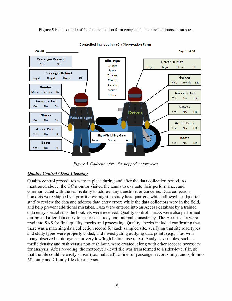
Figure 5 is an example of the data collection form completed at controlled intersection sites.

Figure 5. Collection form for stopped motorcycles.

Quality Control / Data Cleaning Quality control procedures were in place during and after the data collection period. As mentioned above, the QC monitor visited the teams to evaluate their performance, and communicated with the teams daily to address any questions or concerns. Data collection booklets were shipped via priority overnight to study headquarters, which allowed headquarter staff to review the data and address data entry errors while the data collectors were in the field, and help prevent additional mistakes. Data were entered into an Access database by a trained data entry specialist as the booklets were received. Quality control checks were also performed during and after data entry to ensure accuracy and internal consistency. The Access data were read into SAS for final quality checks and processing. Quality checks included confirming that there was a matching data collection record for each sampled site, verifying that site road types and study types were properly coded, and investigating outlying data points (e.g., sites with many observed motorcycles, or very low/high helmet use rates). Analysis variables, such as traffic density and rush versus non-rush hour, were created, along with other recodes necessary for analysis. After recoding, the motorcycle-level file was transformed to a rider-level file, so that the file could be easily subset (i.e., reduced) to rider or passenger records only, and split into MT-only and CI-only files for analysis.

19

Analysis The methodology at the MT study and the CI study level was designed to obtain the data needed to address the following questions.

• What was the DOT-compliant helmet use rate for motorcyclists? • What was the DOT-compliant helmet use rate for motorcycle passengers? • What percentage of motorcycle operators and passengers wore:

o protective gloves? o protective boots? o armored jackets, or armored chest and arm clothing? o armored pants? o high-visibility colors and/or retroreflective material?

The analysis addressed the overall use rate of safety gear and subgroup use, by motorcycle type, road type, day of week, time of day, traffic density, traffic speed, gender, and region.

Weighting The main source of variance in the Round One estimates was the highly clustered and rare nature of this population. As noted above, the study design used a two-phase stratified sample, with sites selected proportional to road segment length. Define:

g – Subscript for region (1 to 4) h – Subscript for road segment stratum (“Best Rides” or Other) i – Subscript for road segment

The Phase I inclusion probability for each observed motorcycle can be expressed as the product of selection probabilities at both stages: 𝜋𝜋𝑔𝑔 for region, and 𝜋𝜋𝑖𝑖|ℎ𝑔𝑔 for road segment i within stratum h; with 𝜋𝜋𝑖𝑖|ℎ𝑔𝑔 being proportional to road segment length within each region and stratum. However, since all four regions were taken with certainty, 𝜋𝜋𝑔𝑔=1. In Phase II, a subsample of road segments was selected from the original sample of non-“Best Rides” road segments within each region, leading to a Phase II probability of selection of one for all “Best Rides” road segments, and less than one for all other road segments. So, the overall inclusion probability for each site is simply the product of:

𝜋𝜋𝑔𝑔ℎ𝑖𝑖 = 𝜋𝜋𝑔𝑔 ∗ 𝜋𝜋ℎ|𝑔𝑔 ∗ 𝜋𝜋𝑖𝑖|ℎ𝑔𝑔

where 𝜋𝜋ℎ|𝑔𝑔, the Phase II probability of selection for each stratum within each region, is equal to one for all “Best Rides” strata. The sampling base weight (design weight) for each site i is the inverse of the probability of inclusion:12

12 An additional time and distance traveled adjustment, like the factor of length over speed used in Brick and Lago

(1988) and a weighting factor used in NOPUS, was also considered. However, the main source of variance in these estimates is the highly clustered and rare nature of this population. The time/distance traveled adjustment is useful in NOPUS because all vehicles are observed and because observation time varies by site type, but had a negligible impact on estimates in this study. Practically, because the end goal is to produce a methodology that is (cont. from page 27) accessible to all states, we wanted to avoid unnecessary complication. Additional weighting factors can be complicated to reproduce correctly, and the resulting time-based estimator (such as is used in NOPUS) can also be challenging to interpret properly. Straightforward weighting adjustments and a simple estimator seemed to best serve the study goals.

20

𝑤𝑤𝑔𝑔ℎ𝑖𝑖 =1𝜋𝜋𝑔𝑔ℎ𝑖𝑖

Table 8 provides descriptive statistics for the site-level base weights overall, and by road type and region. Some of the base weights are quite large, and there is substantial variability even within road type and region. The variability is mostly due to variation in road segment length; because 𝜋𝜋𝑖𝑖|ℎ𝑔𝑔 is proportional to road segment length, very short road segments received very large weights, and vice versa. The coefficient of variation of the weights, which is the standard deviation divided by the mean, is included as an additional measure of variability.

Table 8. Descriptive statistics for Round One moving traffic study base weights

Weight Type Min Median Mean Max CV

Overall 7.2 489.9 3822.9 70257.6 2.08

Road Type

“Best Rides” 7.2 90.5 124.8 433.0 0.87

LAH 17.5 183.5 298.5 1075.3 3.63

Arterials 19.5 373.9 1977.3 70257.6 0.94

Local Roads 250.2 6257.1 9846.8 54186.8 0.93

Region

1 15.6 143.2 1101.1 15269.2 2.38

2 19.6 1414.7 5713.4 54186.8 1.54

3 26.5 551.3 2788.1 25214.3 1.79

4 7.2 512.5 5689.0 70257.6 2.01

While NOPUS data demonstrates that helmet use rates vary by urbanicity, traffic speed, and traffic density (NCSA, 2020), helmet use data are not collected for the CI study in NOPUS. As such there is no data suggesting whether the CI helmet use rate differs from the MT helmet use rate.

In the current study, the MT helmet use rate is based on a larger sample of road segments and observations than the CI helmet use rate, so MT study estimates are assumed to be the most reliable. The CI component of the study is included because detailed observations about PPE use are only possible when the motorcycle is stopped. Therefore, CI observations were only collected at intersections with a stop sign or stop light. Low-traffic and rural areas, or long stretches of road with no traffic control devices, are underrepresented in the CI data. Since the CI study collects data at a non-random subset of the selected sites (only those sites with controlled intersections), and on a possibly non-random subset of motorcycles at those sites (only those motorcycles that stop at the intersection in response to a traffic control device), there is potential for bias in the CI estimates, and an additional weighting step was necessary. We considered the MT study estimate the “gold standard” and created a weighting calibration factor

21

so that the overall CI helmet use estimate, using the weights after calibration, matched the overall MT helmet use estimate.

First, adjustment cells were formed by using a classification tree in SAS’s PROC HPSPLIT to determine which factors were the most important predictors of DOT-compliant helmet use. We crossed those factors and collapsed cells as necessary to produce adjustment cells with large enough sample sizes in both studies; in general, a minimum of five cases in each study. Let ℎ𝑐𝑐𝑀𝑀𝑀𝑀 be the weighted MT helmet use rate within cell c, and let ℎ𝑐𝑐𝐶𝐶𝐶𝐶 be the weighted CI helmet use rate within cell c. The adjustment factor for cell c can then be written as:

𝑓𝑓𝑐𝑐 = ℎ𝑐𝑐𝑀𝑀𝑀𝑀

ℎ𝑐𝑐𝐶𝐶𝐶𝐶

In some cases, adjustment cells were further collapsed to avoid extreme adjustment factors (less than 0.2 or greater than 5). The mean adjustment factor in Round One was 1.85, reflecting that helmet use rates were somewhat higher in most cells in the MT study. The adjusted controlled intersection site base weights for site i in adjustment cell c are then:

𝑤𝑤𝑔𝑔ℎ𝑖𝑖′ = 𝑓𝑓𝑐𝑐 ∗ 𝑤𝑤𝑔𝑔ℎ𝑖𝑖

After benchmarking, the overall controlled CI helmet use rate is identical to the MT helmet use rate. However, use rates for subgroups may differ, and bias in estimates of other PPE use is likely reduced. A set of 288 jackknife replicate weights were also generated for variance estimation purposes, using the MT site base weights. For the CI study, the adjustment factor was applied to each of the replicate weights.

Round One Findings

Observation Sample Sizes and Precision The two-phase sample of 288 road segments produced 741 motorcycles observed, 841 motorcyclists observed (operators and passengers combined), and a mean DOT-certified helmet use rate of 43.03%. The 95% confidence interval was 15.02 to 76.34%. Table 9 provides the actual sample design characteristics and observation sample sizes, and Table 10 provides the actual precision.

Table 9. Sample design characteristics and observation sample sizes

Road Type Road Segments (n) Motorcycles observed per site (k) Yield (n*k)

“Best Rides” 40 6.05 242

LAH 33 1.52 50

Arterials 131 3.38 443

Local Roads 84 0.07 6

Total 288 2.57 741

22

Table 10. Actual precision

P n Var Ste RSE LCI UCI

43.03% 841 0.0305 0.1745 40.55% 15.02% 76.34%

All contingency tables and chi-squared tests were performed using SAS’s PROC SURVEYFREQ, and SAS’s PROC SURVEYREG was used to compute the correlation between operator and passenger helmet use.

Helmet Use Selected findings from Round One MT and CI surveys are presented in Table 11. The overall DOT-compliant helmet use rate estimate in Round One was 43.03% among all motorcyclists and 44.79% among operators, which is lower than the expected rate of 50%, based on the Florida report discussed above. Use rates tended to be higher in regions 1 and 3, and among motorcyclists on LAHs, but lower in regions 2 and 4, and for motorcyclists on non-“Best Rides” arterials. Although local roads appear to have higher helmet use rates, the sample size is so small, with a total of 6 operators observed, that the estimate must be interpreted with extreme caution.

Table 11. Round One moving traffic survey results

All Motorcyclists Operators Only DOT-Compliant Helmet Use Rate

(%)

Standard Error (%) N

DOT-Compliant Helmet Use Rate

(%)

Standard Error (%) N

Overall 43.03 17.45 841 44.79 18.16 741 Region 1 74.45 4.40 315 73.62 4.38 273 2 30.88 6.61 127 28.98 6.48 111 3 61.72 6.46 235 64.19 5.50 209 4 40.11 35.82 164 42.85 37.71 148

Road Type LAH 67.11 11.91 52 65.72 12.57 50 Arterials 40.56 20.29 500 42.35 21.40 443 Local Roads 90.55 11.61 6 90.55 11.61 6 “Best Rides” 63.97 12.00 283 66.01 10.21 242

Note that many of these estimates are associated with very large standard errors. The standard error for region 4 is particularly striking (35.82%), especially since the standard errors for the remaining three regions are in the 4%-7% range. The overall helmet use rate standard error of nearly 18.16% is also much larger than expected.

Despite the higher-than-expected yield of 741 motorcycles and 841 motorcyclists, the Round One design has greater variability than desired. This variability is related to the variability in the base weights shown in Table 8, and point to limitations of the Round One design and a need to determine a remedy for the design in Round Two.

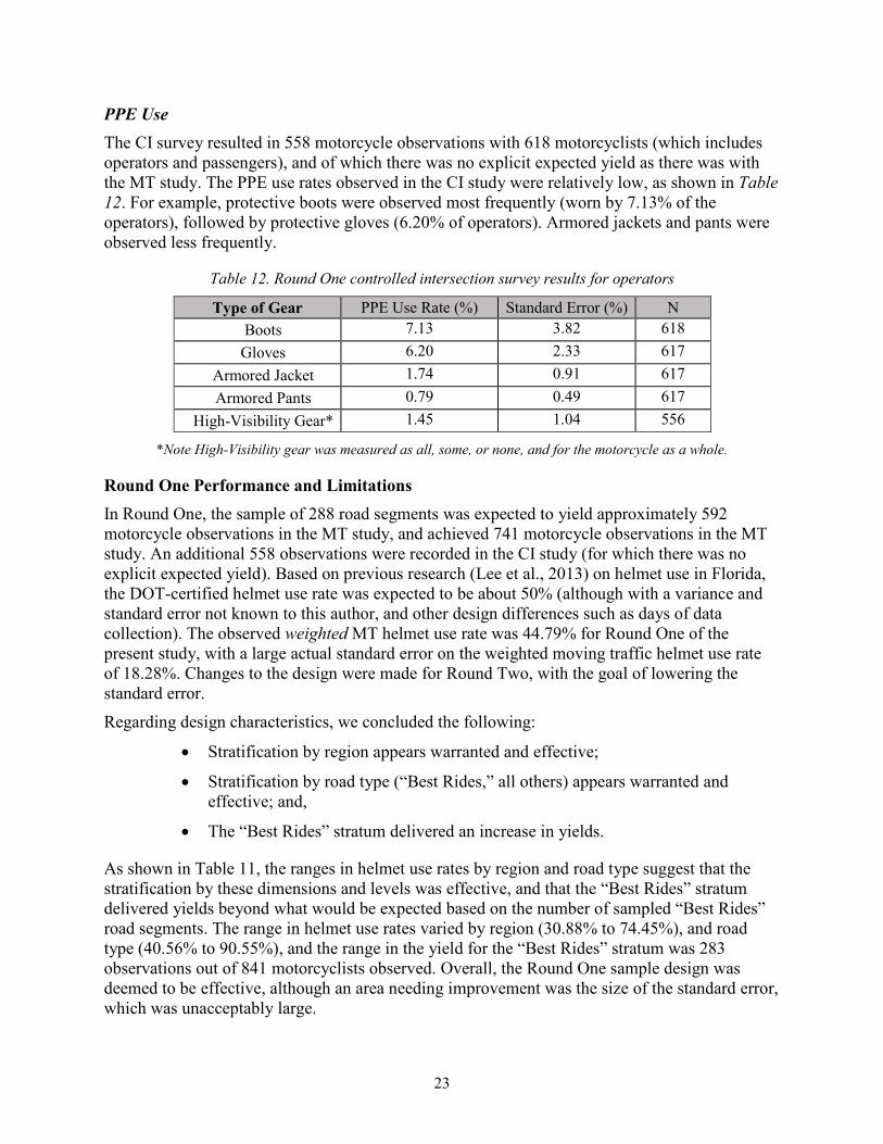
23

PPE Use The CI survey resulted in 558 motorcycle observations with 618 motorcyclists (which includes operators and passengers), and of which there was no explicit expected yield as there was with the MT study. The PPE use rates observed in the CI study were relatively low, as shown in Table 12. For example, protective boots were observed most frequently (worn by 7.13% of the operators), followed by protective gloves (6.20% of operators). Armored jackets and pants were observed less frequently.

Table 12. Round One controlled intersection survey results for operators

Type of Gear PPE Use Rate (%) Standard Error (%) N Boots 7.13 3.82 618

Gloves 6.20 2.33 617 Armored Jacket 1.74 0.91 617 Armored Pants 0.79 0.49 617

High-Visibility Gear* 1.45 1.04 556

*Note High-Visibility gear was measured as all, some, or none, and for the motorcycle as a whole.

Round One Performance and Limitations In Round One, the sample of 288 road segments was expected to yield approximately 592 motorcycle observations in the MT study, and achieved 741 motorcycle observations in the MT study. An additional 558 observations were recorded in the CI study (for which there was no explicit expected yield). Based on previous research (Lee et al., 2013) on helmet use in Florida, the DOT-certified helmet use rate was expected to be about 50% (although with a variance and standard error not known to this author, and other design differences such as days of data collection). The observed weighted MT helmet use rate was 44.79% for Round One of the present study, with a large actual standard error on the weighted moving traffic helmet use rate of 18.28%. Changes to the design were made for Round Two, with the goal of lowering the standard error.

Regarding design characteristics, we concluded the following:

• Stratification by region appears warranted and effective;

• Stratification by road type (“Best Rides,” all others) appears warranted and effective; and,

• The “Best Rides” stratum delivered an increase in yields.

As shown in Table 11, the ranges in helmet use rates by region and road type suggest that the stratification by these dimensions and levels was effective, and that the “Best Rides” stratum delivered yields beyond what would be expected based on the number of sampled “Best Rides” road segments. The range in helmet use rates varied by region (30.88% to 74.45%), and road type (40.56% to 90.55%), and the range in the yield for the “Best Rides” stratum was 283 observations out of 841 motorcyclists observed. Overall, the Round One sample design was deemed to be effective, although an area needing improvement was the size of the standard error, which was unacceptably large.

24

Round Two of Data Collection Road segment length has been used as an MOS in NHTSA’s observation studies since the selection of TIGER as a sampling frame for the Uniform Criteria for State Observational Surveys of Seat Belt Use. As previously noted, the study statisticians have historically expressed concern over the relationship between road segment length and traffic volume. In general, the relationship seems reasonable and useful, as evidenced by the increased precision in estimates obtained with the redesigned NOPUS, which among other things uses length as a measure of size. However, motorcycles on roadways are relatively rare. Motorcyclists may travel in clusters, and with larger than usual intra-class correlations on helmet use, segment length may not be as useful as a MOS under these conditions, and it may indeed cause unnecessary variation in weights that does not cancel with volume. In Round One, two road segments having very large weights, relatively large numbers of motorcycles observed, and unusual helmet use rates had an undesirably large effect on the overall variances and standard errors.

Drawing an equal probability sample of road segments within stratum (region x road type (“Best Rides,” all others)) would reduce the variation in weights considerably, so the Round Two sample was drawn accordingly. The anticipated reward included increased precision. The risks included decreased yields, since it is reasonable to expect that returning to the same road segment sample as used in Round One, would yield similar results for Round Two. Selecting a new sample using an equal probability approach within stratum may result in fewer observations. Given the overall success of the data collection protocol in Round One, we believed the risk of altering the sampling approach was worth the potential reward in Round Two. Methodology For Round Two of the present Pilot Study, the sampling plan and methodology applied similar considerations as that in Round One, except for using PPS, where the MOS was a function of road segment length. The variance of Round One estimates was high, in part due to a very few, very influential, short (i.e., in length) road segments that carried large weights which combined with unusual counts of observations. Thus, an equal probability within road segment stratum design was employed in Round Two, to avoid large variation in weights.

The following sections convey the details of the Round Two sample design characteristics, from sample allocation and optimization, to the expected overall road segment and precision estimates.

Sample Design and Scheduling Based on the findings from Round One, a stratified, single stage, two-phase probability sample of road segments was employed for Round Two. The road segments were selected with equal probability of selection method within stratum. The Round Two sample of 288 road segments in 27 counties was expected to yield 667 motorcycle observations. The total number of motorcyclists observed was expected to be slightly higher, since some motorcycles will have both a rider and a passenger. The Round Two the population of inference, sampling frame, target population and exclusions remain unchanged from Round One.

25

Stratification and Stages of Selection As in Round One, the same 27 Florida counties were in the sample per the FARS criterion. Their geographic distribution was grouped into four regions, and each region was assigned one data collection team (two team members). Given the geographic distribution of counties within each region, it was decided that the sampling of counties within region was unnecessary. Therefore, a stratified, single stage sample of road segments was used. For Round Two, prior to sample selection, the road segments were stratified by road type into four levels (“Best Rides,” LAH, ART, LOC) and sorted by region, county, detailed road type, and a spatial sort such that adjacent road segments on the same road were sequential in the list frame. The road segments were selected with equal probability within stratum to achieve specific target sample sizes by road type stratum.

Road Segment Allocation and Optimization The target sample sizes by road type were adjusted relative to Round One, slightly increasing the “Best Rides” and arterial road segment sample sizes with an eye to increasing the sample and study yields. The total number of “Best Rides” road segments was again fixed at 40 (out of 60 possible “Best Rides” road segments). Table 13 presents the results of that allocation.

Table 13. Optimized road segment sample allocation

Road type Road segment sample size “Best Rides” 60

Limited Access Highways (LAH) 24 Arterials (ART) 145

Local Roads (LOC) 59 Total 288

Road Type Misclassification and Two-Phase Sampling Based on our experience in Round One, we anticipated issues regarding TIGER road type misclassification, and in response, employed a two-phase sample. Given the Round Two allocation, the same Phase I inflation factor was used to obtain the Round Two Phase I sample size, as presented in Table 14.

Table 14. Expected Phase I road segment sample sizes

Road type Road segment sample size “Best Rides” 60

Limited Access Highways (LAH) 32 Arterials (ART) 160

Local Roads (LOC) 100 Total 352

Prior to sample selection, the road segments were stratified by road type (four levels: “Best Rides,” LAH, ART, LOC) and sorted in the following order: by region, county, detailed road type (LAH, ART, LOC), and a spatial sort such that adjacent road segments on the same road were sequential in the list frame. Once the Phase I sample was selected, the TIGER road type was reviewed and updated through a home-office assessment using GIS overlays with TomTom

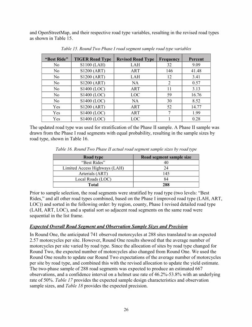
26

and OpenStreetMap, and their respective road type variables, resulting in the revised road types as shown in Table 15.

Table 15. Round Two Phase I road segment sample road type variables

“Best Ride” TIGER Road Type Revised Road Type Frequency Percent No S1100 (LAH) LAH 32 9.09 No S1200 (ART) ART 146 41.48 No S1200 (ART) LAH 12 3.41 No S1200 (ART) NA 2 0.57 No S1400 (LOC) ART 11 3.13 No S1400 (LOC) LOC 59 16.76 No S1400 (LOC) NA 30 8.52 Yes S1200 (ART) ART 52 14.77 Yes S1400 (LOC) ART 7 1.99 Yes S1400 (LOC) LOC 1 0.28

The updated road type was used for stratification of the Phase II sample. A Phase II sample was drawn from the Phase I road segments with equal probability, resulting in the sample sizes by road type, shown in Table 16.

Table 16. Round Two Phase II actual road segment sample sizes by road type

Road type Road segment sample size “Best Rides” 40

Limited Access Highways (LAH) 24 Arterials (ART) 145

Local Roads (LOC) 84 Total 288

Prior to sample selection, the road segments were stratified by road type (two levels: “Best Rides,” and all other road types combined, based on the Phase I improved road type (LAH, ART, LOC)) and sorted in the following order: by region, county, Phase I revised detailed road type (LAH, ART, LOC), and a spatial sort so adjacent road segments on the same road were sequential in the list frame.

Expected Overall Road Segment and Observation Sample Sizes and Precision In Round One, the anticipated 741 observed motorcycles at 288 sites translated to an expected 2.57 motorcycles per site. However, Round One results showed that the average number of motorcycles per site varied by road type. Since the allocation of sites by road type changed for Round Two, the expected number of motorcycles also changed from Round One. We used the Round One results to update our Round Two expectations of the average number of motorcycles per site by road type, and combined this with the revised allocation to update the yield estimate. The two-phase sample of 288 road segments was expected to produce an estimated 667 observations, and a confidence interval on a helmet use rate of 46.2%-53.8% with an underlying rate of 50%. Table 17 provides the expected sample design characteristics and observation sample sizes, and Table 18 provides the expected precision.

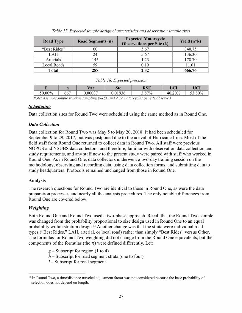
27

Table 17. Expected sample design characteristics and observation sample sizes

Road Type Road Segments (n) Expected Motorcycle Observations per Site (k) Yield (n*k)

“Best Rides” 60 5.67 340.75 LAH 24 5.67 136.30

Arterials 145 1.23 178.70 Local Roads 59 0.19 11.01

Total 288 2.32 666.76

Table 18. Expected precision

P n Var Ste RSE LCI UCI 50.00% 667 0.00037 0.01936 3.87% 46.20% 53.80%

Note: Assumes simple random sampling (SRS), and 2.32 motorcycles per site observed.

Scheduling Data collection sites for Round Two were scheduled using the same method as in Round One.

Data Collection Data collection for Round Two was May 5 to May 20, 2018. It had been scheduled for September 9 to 29, 2017, but was postponed due to the arrival of Hurricane Irma. Most of the field staff from Round One returned to collect data in Round Two. All staff were previous NOPUS and NSUBS data collectors; and therefore, familiar with observation data collection and study requirements, and any staff new to the present study were paired with staff who worked in Round One. As in Round One, data collectors underwent a two-day training session on the methodology, observing and recording data, using data collection forms, and submitting data to study headquarters. Protocols remained unchanged from those in Round One.

Analysis The research questions for Round Two are identical to those in Round One, as were the data preparation processes and nearly all the analysis procedures. The only notable differences from Round One are covered below.

Weighting Both Round One and Round Two used a two-phase approach. Recall that the Round Two sample was changed from the probability proportional to size design used in Round One to an equal probability within stratum design.13 Another change was that the strata were individual road types (“Best Rides,” LAH, arterial, or local road) rather than simply “Best Rides” versus Other. The formulas for Round Two weighting did not change from the Round One equivalents, but the components of the formulas (the 𝜋𝜋) were defined differently. Let:

g – Subscript for region (1 to 4) h – Subscript for road segment strata (one to four) i – Subscript for road segment

13 In Round Two, a time/distance traveled adjustment factor was not considered because the base probability of

selection does not depend on length.

28

As in Round One, the Phase I inclusion probability for each observed motorcycle is the product of selection probabilities at both stages: 𝜋𝜋𝑔𝑔 for region, 𝜋𝜋𝑖𝑖|ℎ𝑔𝑔 for road segment i within stratum h. In Round Two, the road segment-level probability, 𝜋𝜋𝑖𝑖|ℎ𝑔𝑔, is constant within region and stratum. Since all four regions were taken with certainty, set 𝜋𝜋𝑔𝑔=1 for all regions. In Phase II, a subsample of road segments was selected from the original sample of non-“Best Rides” road segments within each region, leading to a Phase II probability of selection of one for all “Best Rides” road segments, and less than one otherwise. The overall inclusion probability for each site is the product of:

𝜋𝜋𝑔𝑔ℎ𝑖𝑖 = 𝜋𝜋𝑔𝑔 ∗ 𝜋𝜋ℎ|𝑔𝑔 ∗ 𝜋𝜋𝑖𝑖|ℎ𝑔𝑔

where 𝜋𝜋ℎ|𝑔𝑔, the Phase II probability of selection for each stratum within each region, is 1 for all “Best Rides” strata. The sampling base weight (design weight) for each site i is the inverse of the probability of inclusion:

𝑤𝑤𝑔𝑔ℎ𝑖𝑖 =1𝜋𝜋𝑔𝑔ℎ𝑖𝑖

Table 19 provides descriptive statistics for the site-level base weights overall and by road type and region. Compared to the Round One weights, the Round Two weights are much less variable; for example, in Round One, the largest weight of 70,258 was about 10,000 times larger than the smallest weight (7.2), while in Round Two, the largest weight of 16,962 is about 170 times larger than the smallest weight (99.5). This change is also reflected in smaller CVs. These less-variable weights should result in standard errors on the estimates that are lower than those for the Round One estimates. (The base weight for one site that had been sampled as a local road but then reclassified as an arterial, was trimmed back to the median base weight for arterials (559.8).)

Table 19. Round Two moving traffic survey, descriptive statistics base weights

Base Weigh Min Median Mean Max CV Overall 99.5 559.8 2615.5 16962.0 1.73 Road Type Best Rides 116.6 608.2 164.3 228.9 0.29 LAHs 99.5 608.2 581.6 1125.3 0.56 Arterials 263.5 559.8 1113.2 16962.0 2.54 Local roads 3124.2 9815.3 9627.6 15265.8 0.44

Region 1 99.5 263.5 825.1 3453.1 1.47 2 228.9 559.8 4253.2 16962.0 1.55 3 191.6 563.9 2753.9 10259.7 1.43 4 116.6 481.2 2629.8 10088.0 1.54

As in Round One, the CI weights were benchmarked so that the CI helmet use rate is identical to the MT helmet use rate; a set of 288 jackknife replicate weights were again generated for variance estimation purposes for both studies.

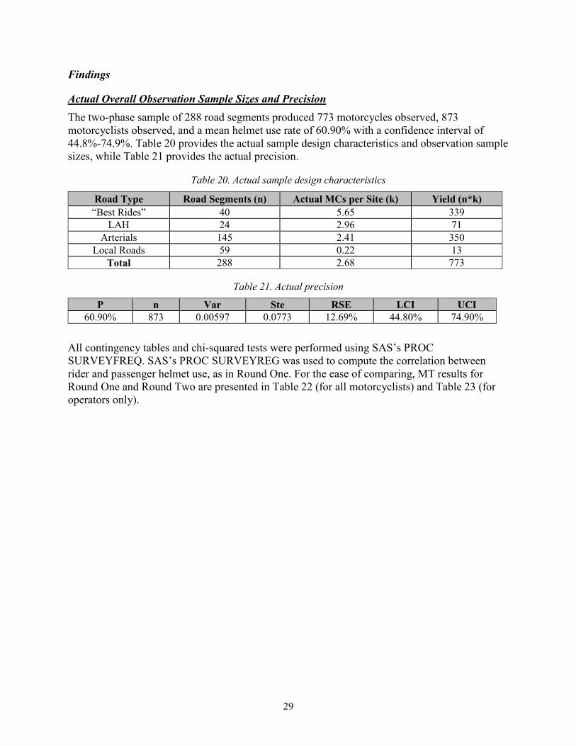
29

Findings

Actual Overall Observation Sample Sizes and Precision The two-phase sample of 288 road segments produced 773 motorcycles observed, 873 motorcyclists observed, and a mean helmet use rate of 60.90% with a confidence interval of 44.8%-74.9%. Table 20 provides the actual sample design characteristics and observation sample sizes, while Table 21 provides the actual precision.

Table 20. Actual sample design characteristics

Road Type Road Segments (n) Actual MCs per Site (k) Yield (n*k) “Best Rides” 40 5.65 339

LAH 24 2.96 71 Arterials 145 2.41 350

Local Roads 59 0.22 13 Total 288 2.68 773

Table 21. Actual precision

P n Var Ste RSE LCI UCI 60.90% 873 0.00597 0.0773 12.69% 44.80% 74.90%

All contingency tables and chi-squared tests were performed using SAS’s PROC SURVEYFREQ. SAS’s PROC SURVEYREG was used to compute the correlation between rider and passenger helmet use, as in Round One. For the ease of comparing, MT results for Round One and Round Two are presented in Table 22 (for all motorcyclists) and Table 23 (for operators only).

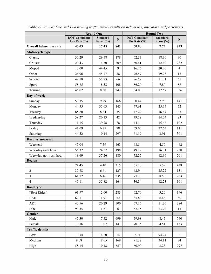
30

Table 22. Rounds One and Two moving traffic survey results on helmet use, operators and passengers Round One Round Two

DOT-Compliant Use Rate (%)

Standard Error (%) N DOT-Compliant

Use Rate (%) Standard Error (%) N

Overall helmet use rate 43.03 17.45 841 60.90 7.73 873

Motorcycle type

Classic 30.29 29.58 178 62.33 18.30 90 Cruiser 23.43 14.30 209 60.41 12.40 282 Moped 17.00 44.45 9 16.76 20.76 4 Other 26.96 45.77 28 76.57 19.98 12 Scooter 49.18 55.83 66 26.52 11.31 61 Sport 58.85 18.58 108 86.20 7.80 88 Touring 45.02 8.30 243 64.00 12.57 336

Day of week

Sunday 53.35 9.29 166 80.44 7.96 141 Monday 44.55 35.03 145 47.61 25.35 72 Tuesday 85.80 8.34 35 42.29 16.67 63 Wednesday 39.27 20.13 42 79.28 14.34 83 Thursday 11.15 39.78 78 44.14 15.46 102 Friday 41.09 6.25 78 59.03 27.63 111 Saturday 44.52 10.14 297 61.19 3.91 301

Rush vs. non-rush

Weekend 47.04 7.59 463 68.54 4.50 442 Weekday rush hour 56.32 24.27 198 49.12 16.01 230 Weekday non-rush hour 18.69 37.26 180 72.25 12.96 201

Region

1 74.45 4.40 315 65.20 5.59 438 2 30.88 6.61 127 42.94 25.22 131 3 61.72 6.46 235 77.70 8.50 203 4 40.11 35.82 164 36.34 12.23 101

Road type

“Best Rides” 63.97 12.00 283 62.70 3.20 396 LAH 67.11 11.91 52 85.80 6.46 80 ART 40.56 20.29 500 57.16 11.26 384 LOC 90.55 11.61 6 62.75 23.70 13

Gender Male 47.30 17.52 699 59.98 8.47 740 Female 19.36 13.07 141 70.35 4.51 133

Traffic density

Low 10.34 14.20 14 2.71 94.24 2 Medium 9.08 18.65 169 71.32 34.11 74 High 58.14 10.48 657 60.90 8.23 797

31

Table 23. Rounds One and Two moving traffic survey results on helmet use, operators only

Round One Round Two DOT-Compliant

Use Rate (%) Standard Error (%) N DOT-Compliant

Use Rate (%) Standard Error (%) N

Overall helmet use rate 44.79 18.16 741 60.55 8.25 773 Motorcycle type

Classic 29.05 30.73 158 62.79 18.93 85 Cruiser 27.70 11.13 186 60.44 13.31 250 Moped 17.00 44.45 9 16.76 20.76 4 Other 25.43 53.81 24 69.66 22.68 9 Scooter 51.72 55.78 62 25.57 11.04 60 Sport 58.78 18.53 106 86.20 7.80 88 Touring 43.16 8.63 196 63.42 14.30 277

Day of week

Sunday 55.36 9.70 133 80.73 8.85 122 Monday 45.84 34.98 134 47.01 25.94 67 Tuesday 86.24 8.24 34 42.60 17.71 57 Wednesday 39.18 20.16 41 79.12 15.53 75 Thursday 18.14 33.40 72 44.70 16.18 97 Friday 36.11 4.13 71 58.18 28.24 105 Saturday 44.95 10.42 256 62.01 3.97 250

Rush vs. non-rush

Weekend 47.94 7.88 389 69.29 4.82 372 Weekday rush hour 59.16 21.02 186 48.66 16.33 218 Weekday non-rush hour 18.56 36.04 166 72.34 13.67 183

Region

1 73.62 4.38 273 64.49 5.90 382 2 28.98 6.48 111 40.89 26.57 118 3 64.19 5.50 209 78.12 8.85 183 4 42.85 37.71 148 36.69 13.08 90

Road type

“Best Rides” 66.01 10.21 242 63.08 3.17 339 LAH 65.72 12.57 50 85.73 6.59 71 ART 42.35 21.40 443 56.44 12.05 350 LOC 90.55 11.61 6 62.75 23.70 13

Gender Male 47.39 17.53 695 60.08 8.49 737 Female 14.47 16.92 46 76.08 7.99 36

Traffic density

Low 1.63 2.87 11 2.71 94.24 2 Medium 9.58 20.14 143 72.62 35.43 63 High 60.11 8.96 586 60.32 8.82 708

32

In Round One, 741 motorcycles and 841 total motorcyclists were observed, compared to 773 motorcycles and 873 total motorcyclists in Round Two; this outcome indicates that the change in design did not negatively affect the yield in observations. The overall DOT-compliant helmet use rate increased from 43.03% to 60.90%, and from 44.79% to 60.55% for all motorcyclists. As expected, the standard errors decreased substantially under the Round Two design, dropping by about 10 percentage points for all motorcyclists and for operators only. Although the estimated use rates appear to be higher in Round Two than in they are in Round One, there is no statistically significant difference between the Round One and Round Two estimates, due to the large uncertainty in the Round One estimate. For example, the Round One 95-percent CI for DOT-compliant helmet use among all operators was 15.0% to 76.3%; in contrast, the Round Two 95-percent CI was 44.8% to 74.9%.

The correlation between operator and passenger DOT-compliant helmet use was 94.66% in Round One and 92.27% in Round Two, indicating that the clear majority of passengers had the same helmet use status as the operator; a helmeted operator is very likely to have a helmeted passenger, and similarly for unhelmeted operators.

In both Round One and Round Two, we see higher helmet use rates in regions 1 and 3, and lower rates in regions 2 and 4; the differences are statistically significant between region 2 and regions 1 (p<0.0001) and 3 (p=0.0022) in Round One, and between region 4 and regions 1 (p=0.0335) and 3 (p=0.00618) in Round Two. Helmet use rates are also higher on LAHs and “Best Rides” in both rounds, but only the Round Two helmet use rate on LAHs is significantly higher than the use rate for Round Two on arterials (p=0.0289) or “Best Rides” (p=0.0017). The number of operators observed on local roads was too small for reliable inference. An additional statistically significant difference found was between Round One Medium and High-Density traffic volumes (p=0.0151), but not in Round Two. There were no statistically significant differences found between gender or rush-hour versus non-rush hour in either Round One or Round Two.

There was variation in the number of motorcyclists observed and helmet use rates by type of motorcycle and the day of week. This variation is partially due to the relatively small cell sizes for many motorcycle types and days of the week, and underscores that motorcyclists are a rare and inherently variable population.

The number of motorcycles observed in the controlled intersection studies was lower in both rounds compared to the number observed in the moving traffic studies: 557 motorcycles and 619 motorcyclists in Round One, and 602 motorcycles with 674 motorcyclists in Round Two. This finding was expected, since the controlled intersection studies observed a subset of motorcycles traveling on the sampled road segments because observations.

Helmet Use in Controlled Intersection Study Due to benchmarking, the DOT-compliant helmet use rates observed in the CI studies for all motorcyclists are identical to those in the MT studies. In addition, the patterns of helmet use rates for the CI studies are like those in the MT studies, for Round One and Two. This finding is expected, since the MT and CI studies are performed at the same sites and similar times. It also indicates that the data collectors accurately observed motorcycle type and helmet use in the MT study. The CI study results for each round are shown in Table 24, for all motorcyclists, and Table 25, for operators only.

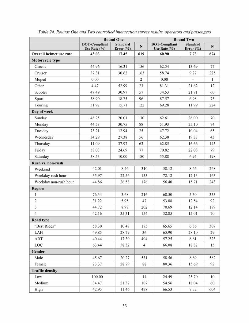
33

Table 24. Rounds One and Two controlled intersection survey results, operators and passengers

Round One Round Two DOT-Compliant

Use Rate (%) Standard Error (%) N DOT-Compliant

Use Rate (%) Standard Error (%) N

Overall helmet use rate 43.03 17.45 619 60.90 7.73 674 Motorcycle type

Classic 44.96 16.31 156 62.54 13.69 77 Cruiser 37.31 30.62 163 58.74 9.27 225 Moped 0.00 - 2 0.00 - 1 Other 4.47 52.99 23 81.31 21.62 12 Scooter 47.49 30.97 57 34.53 21.81 60 Sport 58.90 18.75 96 87.57 6.98 75 Touring 31.92 15.71 122 69.28 11.99 224

Day of week

Sunday 48.25 20.01 130 62.61 26.00 70 Monday 44.53 30.75 88 51.93 25.10 74 Tuesday 73.21 12.94 25 47.72 10.04 65 Wednesday 34.29 27.38 56 62.30 19.33 43 Thursday 11.09 37.97 63 62.85 16.66 145 Friday 58.03 24.69 77 70.82 22.08 79 Saturday 38.53 10.00 180 55.88 6.95 198

Rush vs. non-rush

Weekend 42.01 8.46 310 58.12 8.65 268

Weekday rush hour 35.97 22.56 133 72.12 12.13 163 Weekday non-rush hour 44.86 26.58 176 56.40 15.71 243

Region

1 76.34 3.68 216 68.50 5.30 333 2 31.22 5.95 47 53.88 12.54 92 3 44.72 8.98 202 70.69 12.14 179 4 42.16 35.31 154 32.85 15.01 70

Road type

“Best Rides” 58.30 10.47 175 65.65 6.36 307 LAH 49.85 28.79 36 65.90 28.10 29 ART 40.44 17.30 404 57.25 8.61 323 LOC 63.44 58.32 4 66.08 18.32 15

Gender Male 45.67 20.27 531 58.56 8.69 582 Female 23.37 28.79 88 80.36 15.69 92

Traffic density

Low 100.00 - 14 24.49 25.70 10 Medium 34.47 21.37 107 54.56 18.04 60 High 42.95 11.46 498 66.53 7.52 604

34

Table 25. Rounds One and Two controlled intersection survey results, operators only

Round One Round Two

DOT-Compliant Use Rate (%)

Standard Error (%) N DOT-Compliant

Use Rate (%) Standard Error (%) N

Overall helmet use rate 43.65 17.01 557 59.39 8.62 602

Motorcycle type

Classic 43.91 16.37 143 65.29 13.23 72 Cruiser 36.41 32.55 147 53.75 12.65 209 Moped 0.00 - 2 . . 1 Other 4.95 56.33 15 81.35 20.35 8 Scooter 47.51 30.95 56 34.65 21.93 58 Sport 58.75 18.80 95 87.52 7.02 74 Touring 27.98 17.44 99 69.55 13.72 180

Day of week

Sunday 49.61 21.98 114 60.99 28.10 62 Monday 46.50 27.65 84 52.16 25.59 67 Tuesday 73.21 12.94 25 47.84 10.76 57 Wednesday 36.08 30.12 54 65.49 19.42 41 Thursday 10.70 37.37 59 63.11 17.12 135 Friday 58.05 25.45 70 70.98 22.13 77 Saturday 33.75 9.99 151 45.88 14.85 163

Rush vs. non-rush

Weekend 39.46 9.85 265 51.60 12.84 225 Weekday rush hour 35.65 22.97 127 73.59 12.05 155 Weekday non-rush hour 46.61 24.60 165 56.57 16.06 222

Region

1 77.40 3.40 189 67.59 5.62 286 2 28.45 7.71 43 43.57 18.42 85 3 45.42 9.23 184 71.81 12.38 165 4 43.49 34.46 141 33.52 15.83 66

Road type

“Best Rides” 56.98 10.87 148 67.16 6.67 267 LAH 51.51 31.36 35 76.85 17.47 26 ART 41.08 16.75 370 53.26 10.19 294 LOC 63.44 58.32 4 66.08 18.32 15

Gender Male 46.82 18.89 527 58.79 8.73 576 Female 7.96 30.61 30 87.64 7.13 26

Traffic density

Low 100.00 - 13 24.49 0.00 10 Medium 35.55 22.34 93 46.46 24.45 54 High 42.94 11.52 451 67.68 7.74 538

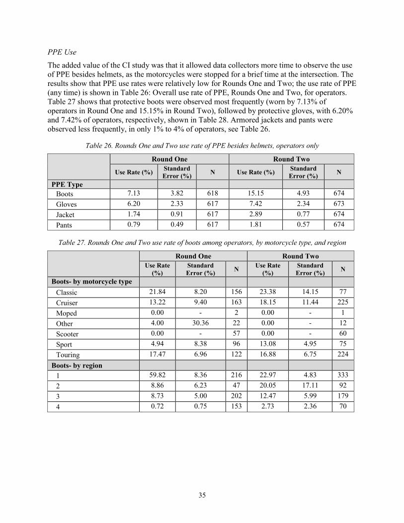
35

PPE Use The added value of the CI study was that it allowed data collectors more time to observe the use of PPE besides helmets, as the motorcycles were stopped for a brief time at the intersection. The results show that PPE use rates were relatively low for Rounds One and Two; the use rate of PPE (any time) is shown in Table 26: Overall use rate of PPE, Rounds One and Two, for operators. Table 27 shows that protective boots were observed most frequently (worn by 7.13% of operators in Round One and 15.15% in Round Two), followed by protective gloves, with 6.20% and 7.42% of operators, respectively, shown in Table 28. Armored jackets and pants were observed less frequently, in only 1% to 4% of operators, see Table 26.

Table 26. Rounds One and Two use rate of PPE besides helmets, operators only

Round One Round Two

Use Rate (%) Standard Error (%) N Use Rate (%) Standard

Error (%) N

PPE Type

Boots 7.13 3.82 618 15.15 4.93 674 Gloves 6.20 2.33 617 7.42 2.34 673 Jacket 1.74 0.91 617 2.89 0.77 674 Pants 0.79 0.49 617 1.81 0.57 674

Table 27. Rounds One and Two use rate of boots among operators, by motorcycle type, and region

Round One Round Two

Use Rate (%)

Standard Error (%) N Use Rate

(%) Standard Error (%) N

Boots- by motorcycle type

Classic 21.84 8.20 156 23.38 14.15 77 Cruiser 13.22 9.40 163 18.15 11.44 225 Moped 0.00 - 2 0.00 - 1 Other 4.00 30.36 22 0.00 - 12 Scooter 0.00 - 57 0.00 - 60 Sport 4.94 8.38 96 13.08 4.95 75 Touring 17.47 6.96 122 16.88 6.75 224

Boots- by region

1 59.82 8.36 216 22.97 4.83 333 2 8.86 6.23 47 20.05 17.11 92 3 8.73 5.00 202 12.47 5.99 179 4 0.72 0.75 153 2.73 2.36 70

36

Table 28. Rounds One and Two use rate of gloves among operators, by motorcycle type, and region Round One Round Two Use Rate

(%) Standard Error (%) N Use Rate

(%) Standard Error (%) N

Gloves- by motorcycle type Classic 13.43 4.56 156 19.14 13.90 77 Cruiser 10.54 8.27 162 3.51 1.45 225 Moped 0.00 - 2 0.00 - 1 Other 1.54 11.89 22 0.00 - 12 Scooter 0.29 0.35 57 0.86 0.83 60 Sport 14.85 8.41 96 14.49 6.30 75 Touring 6.24 4.15 122 7.91 3.20 223

Gloves- by region

1 28.39 5.54 216 15.96 3.63 333 2 4.47 3.47 47 8.75 6.37 92 3 13.32 4.57 202 4.76 4.78 179 4 1.34 1.13 152 0.00 - 69

Table 29. Rounds One and Two use rate of jackets among operators, by motorcycle type and region

Round One Round Two

Use Rate (%)

Standard Error (%) N Use Rate

(%) Standard Error (%) N

Armored Jacket- by motorcycle type

Classic 2.66 1.97 156 0.87 0.57 77 Cruiser 2.18 1.65 162 2.54 1.23 225 Moped 0.00 - 2 0.00 - 1 Other 0.00 - 22 6.67 9.54 12 Scooter 0.00 - 57 0.00 - 60 Sport 5.18 5.10 96 4.62 2.31 75 Touring 2.29 1.59 122 5.79 2.61 224

Armored Jacket- by region

1 15.89 3.55 216 10.71 2.58 333 2 4.30 3.43 47 2.15 1.41 92 3 0.03 0.03 202 0.00 - 179 4 0.41 0.50 152 0.88 0.84 70

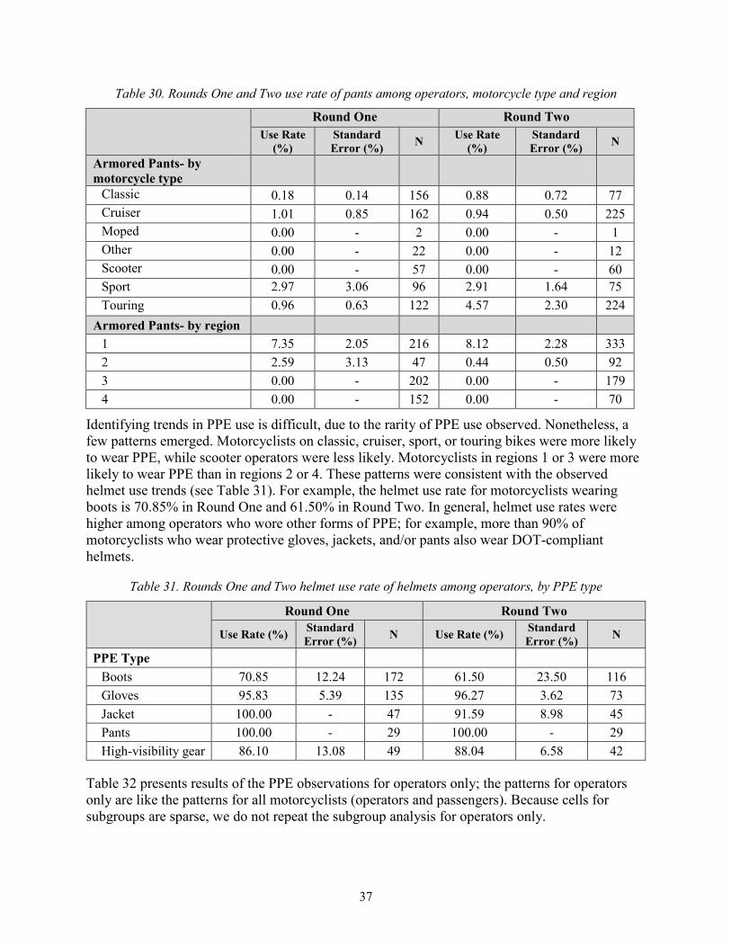
37

Table 30. Rounds One and Two use rate of pants among operators, motorcycle type and region

Round One Round Two Use Rate

(%) Standard Error (%) N Use Rate

(%) Standard Error (%) N

Armored Pants- by motorcycle type

Classic 0.18 0.14 156 0.88 0.72 77 Cruiser 1.01 0.85 162 0.94 0.50 225 Moped 0.00 - 2 0.00 - 1 Other 0.00 - 22 0.00 - 12 Scooter 0.00 - 57 0.00 - 60 Sport 2.97 3.06 96 2.91 1.64 75 Touring 0.96 0.63 122 4.57 2.30 224

Armored Pants- by region

1 7.35 2.05 216 8.12 2.28 333 2 2.59 3.13 47 0.44 0.50 92 3 0.00 - 202 0.00 - 179 4 0.00 - 152 0.00 - 70

Identifying trends in PPE use is difficult, due to the rarity of PPE use observed. Nonetheless, a few patterns emerged. Motorcyclists on classic, cruiser, sport, or touring bikes were more likely to wear PPE, while scooter operators were less likely. Motorcyclists in regions 1 or 3 were more likely to wear PPE than in regions 2 or 4. These patterns were consistent with the observed helmet use trends (see Table 31). For example, the helmet use rate for motorcyclists wearing boots is 70.85% in Round One and 61.50% in Round Two. In general, helmet use rates were higher among operators who wore other forms of PPE; for example, more than 90% of motorcyclists who wear protective gloves, jackets, and/or pants also wear DOT-compliant helmets.

Table 31. Rounds One and Two helmet use rate of helmets among operators, by PPE type

Round One Round Two

Use Rate (%) Standard Error (%) N Use Rate (%) Standard

Error (%) N

PPE Type

Boots 70.85 12.24 172 61.50 23.50 116 Gloves 95.83 5.39 135 96.27 3.62 73 Jacket 100.00 - 47 91.59 8.98 45 Pants 100.00 - 29 100.00 - 29 High-visibility gear 86.10 13.08 49 88.04 6.58 42

Table 32 presents results of the PPE observations for operators only; the patterns for operators only are like the patterns for all motorcyclists (operators and passengers). Because cells for subgroups are sparse, we do not repeat the subgroup analysis for operators only.

38

Table 32. Rounds One and Two controlled intersection survey results of use rate of PPE, operators only

Round One Round Two Use Rate

(%) Std Error

(%) N Use Rate (%) Std Error (%) N

PPE Type

Boots 7.17 4.00 557 15.30 5.78 602

Gloves 6.34 2.48 556 7.75 2.60 601 Jacket 1.78 0.96 556 2.89 0.81 602 Pants 0.80 0.51 556 1.70 0.52 602 High-visibility gear 1.45 1.04 556 4.03 1.18 602

39

Discussion Potential Methodology for States Based on the findings from Rounds One and Two of the present study, which showed relative improvement achieved by adjusting the Round Two sample design by drawing an equal probability sample of road segments within region and road type, we present methods for observation, probability sample studies of motorcycle helmet and PPE use. The methods are categorized as design features, and changes to key information, constraints, and parameters, given the degree to which they may be easily accommodated in a probability design, or the degree to which they may be deviations, respectively.

Identifying and oversampling road segments that are likely to have higher rates of flow, such as the “Best Rides” stratum, is crucial to increasing yields efficiently. However, the ability to overlay different GIS resources is required, and may not be a capability within reach of all possible researchers. For those who do not have the GIS resources to complete such an overlay, oversampling arterial road segments will also help to increase yields. In addition, given the relative rarity of motorcycles, and the weak relationship of such volume to road segment length, the latter should be avoided in PPS designs, as should more generally any designs that results in some sites being assigned larger weights.

Road type misclassification is also a real and identifiable problem with TIGER (and quite likely any/all road segment sampling frames/sources). More extensive frame-based overlay and improvement of road type, two-phase sampling and/or weight trimming are the remedies for this problem.

While a more refined sample design would be possible with better population information related to motorcycle volume by road segment, obtaining such a design is difficult to envision and obtain. Beyond the improvements mentioned above, large increases in observations may only be achieved through large increases in road segment sample sizes. Considerably larger Phase I sample sizes (compared to Phase II) may help with misclassification and help to equalize weights and allow for greater Phase II subsampling. In addition, relaxing the equal workloads per region or other PSU expectation (which is common in observational studies) would work to decrease variability in weights within road type across PSUs. Finally, excluding local roads from the target population could dramatically increase overall yields, given the few observations that occur on local roads even when under sampled, and minimal bias in estimates may result.

The data collectors used paper forms to record their observations during data collection. Given that this observational survey is in its infancy (as the methodology is evolving) and there was likely to be several revisions to the data collection instrument, it was more efficient and cost effective to develop and revise paper instruments. Additionally, it would be more economical to reproduce paper data collection forms, as opposed to electronic data collection methods.

Due to the differences in traffic volume, speed and overall landscape regarding collecting data on surface streets and limited access highways, different data collection methodologies must be employed to maximize the number and accuracy of the observations. That is, observations of moving traffic will only allow the data collector to observe a minimal number of characteristics such as bike type, gender, and helmet use. Conversely, building in time to complete a survey of motorcycles in stopped traffic will allow data collectors to observe PPE in some detail which permits the observation of footwear, pants, gloves, and jackets. It is important to note, however,

40

that in this study fewer observations of motorcyclists were made when observing stopped traffic, so it is not desirable to exclude the moving traffic survey in favor of the stopped traffic survey, conducted at intersections.

It was efficient to collect data in pairs, with one individual serving as a spotter and the other as the recorder. Regarding scheduling data collection sites, it is cost effective to cluster sites within relatively proximity and schedule them accordingly. In addition, while more motorcyclists were observed on weekend days, it is more representative of the entire riding population to obtain data for motorcyclists on both weekends and weekdays. Using this approach will include commuters as well as the recreational motorcyclists.

Comparisons between the present study (referred to as the Pilot Study) and other observational studies like NHTSA’s NOPUS and the Uniform Criteria for State Observational Surveys for Seat Belt Use, can be made on study and sample design characteristics and may prove useful. The Pilot Study adopted a MT and CI data collection protocol, much like those used in NOPUS, to allow for more detailed PPE data collection. However, to our knowledge these protocols are unique to NOPUS and the present Pilot Study. The aforementioned studies used road segment sample designs, either multi-stage or single-stage, and most use TIGER as the source of the road segment sampling frame.14 Many but not all the studies used road segment length, daily vehicle miles traveled, or annual vehicle miles traveled as a measure of size for PPS sampling. The utility of such measures, especially for a rare population like motorcycles, is questionable. The oversampling of arterial road types, and especially the identification of a “Best Rides” stratum and its oversampling, are unique to the present Pilot Study. We believe that the approach taken during Round One, and the improvements in Round Two, take advantage of this body of work while making appropriate modifications, and thereby represents a general state-of-the art approach.

State Specific Surveys Given that States complete annual observational surveys of seat belt use, with a data collection approach and sample design like the one tested in the current study for a motorcycle survey, it is reasonable to conclude that most if not all States could design and conduct their own motorcycle PPE studies. However, there are caveats. First and foremost, the overall expected rate of flow of motorcycles within a State will largely determine if the tested protocol can produce the yields required for reasonable precision. States with large populations, high numbers of registered motorcycles, long riding seasons, etc., will likely have the rate of flow required. The study and sample designs for these States can be made more efficient with the oversampling of arterials and “Best Rides” (when possible) road types. States without large populations, high numbers of registered motorcycles, or long riding seasons may have to rely on increased oversampling, larger road segment sample sizes, longer field periods, and possibly other novel approaches to obtain the yields required for reasonable precision.

When designing and implementing a State-based observation survey of PPE use, the following criteria regarding accuracy and reliability could be used:

14 The Uniform Criteria for State Observational Surveys allows for the States to use their own road databases.

41

Sample Sample Design. The direct selection of road segments is impractical for a PPE use survey that requires human observations of passing-by motorcycles on the selected roads. Although it would be most efficient, data collection cost would be prohibitively expensive. Therefore, a two or three-stage cluster design could be used, where single counties or groups of counties are first selected as the primary sampling units (PSUs – optional depending on the size of a State, its characteristics, and goals of the study), and road segments are then selected from the selected PSUs. At the last stage, motorcycles are observed on the selected roads at a designated time.

Sample Size and Precision. The sample size and precision are directly related, and so are the cost and the sample size. The larger the sample size, the better the precision and the higher the survey cost. Hence, the sample size is determined to minimize the survey cost while meeting the precision requirement.

County or PSU Selection. Selecting counties of various types and with probabilities related to volume will ensure face-validity and work to achieve increased yields, respectively. Stratification within a State by region, urbanicity, and other geographic and demographic characteristics will help ensure face-validity as well as the precision of estimates related to these characteristics. Selecting counties with probability proportional to size, where the measure of size is related to motorcycle registrations or volume will help increase expected yields and increase the precision of estimates.

Road Segment Selection. Selected road segments should be mapped per the latitude and longitude of their midpoints. The selected road segment should be identified by an intersection or interchange that occurs within or just beyond the segment. If no intersection or interchange occurs within the segment, then any point on that road can be used for observation. The observed direction of travel should be randomly assigned for each road segment.

Reserve Sample. Sometimes the sample yield in terms of the observed motorcyclists is below what was projected, resulting in a high risk of not meeting the precision requirement. To avoid this situation, a reserve sample of road segments should be used when the sample yield is low. If the sample yield is not expected to fluctuate too much, selecting 30% more to be used as a reserve sample would be good enough. If the sample size of the road segment sample is 20 per PSU, then it would need to select six more road segments per PSU as the reserve sample.

Data Collection Site Scheduling. Observations should be conducted during weekdays and weekends in daylight. The schedule should include rush hour (before 9:30 a.m. and after 3:30 p.m.) and non-rush hour observations. Time of day/day of week should be balanced to capture recreational motorcyclists versus commuters. Sites within relatively close geographic proximity should be assigned as data collection clusters. Within these clusters, sites should be randomly selected for day of the week/start time. Observations should be conducted during motorcycle riding season, typically April to October, and data should be collected for periods of at least 40 minutes per site to ensure motorcycles are observed.

Recording Observations. Data collection should be performed in teams of two, with one data collector serving as the spotter and one serving as a recorder. Data collectors should observe as many lanes of traffic as s/he can comfortably monitor while being certain that s/he is accurately collecting data on 99% of the motorcycles. Motorcycle Type (Cruiser, Sport, Touring, etc.) and

42

Helmet Definitions (DOT-Compliant, Not Certified, and None) should be clearly defined as well as any additional PPE observed. Data should be collected on all motorcyclists, the operators and any passengers.

Alternate Sites. When a site is temporarily unavailable due to a crash or inclement weather, data collection should be rescheduled for a similar time of day and type of day of week. If the site is permanently unworkable, such as located within a gated community, an alternate site, selected as part of the reserve sample, should be used as a permanent replacement.

Quality Control. A designated QC monitor should make unannounced visits to data collection sites within each PSU. During these visits, the QC monitor should first evaluate the data collectors performance from a distance (if possible), and then work alongside the data collectors. The QC monitor will ensure the data collector is following all survey protocol including: being on time at assigned sites, completing the cover sheet and observation forms, and making accurate observations.

Imputation, Weighting, Point and Variance Estimation Imputation. Given the very low rates of site- and item-level nonresponse in both rounds, and given that imputation can be a complex and burdensome process, imputation is likely unnecessary. Site-level nonresponse should be handled via nonresponse adjustments in survey weighting, discussed in more detail below. If item-level nonresponse is high for some items (greater than 5% is a good rule of thumb), consider using hot-deck imputation.

Sampling Weights. Sampling weights should consist of a base weight that accounts for the probabilities of selection at all levels of selection. This base weight should be available for all sampled sites, and should be strictly greater than zero. The base weight should be multiplied by adjustment factors as necessary, including a nonresponse adjustment. If a controlled intersection-type study is performed at some subset of sites, the sampling weights for controlled intersection sites should be benchmarked to the main study (moving traffic-type) weights.

Non-Response Adjustments. If a site is unworkable and there is no suitable alternate, it becomes a non-responding site. Such sites receive a final weight of zero, and their original base weight should be redistributed over other, similar sites. This should be done by first forming nonresponse cells, which minimally are formed by crossing sampling strata (for example, PSU by road type cells) but can be finer if desired. Within each cell, the weights for non-responding sites are zeroed out, and the weights for all responding sites within the cell are adjusted upwards by a factor greater than one so that the weight total within the cell remains the same after adjustment. This allows the non-responding sites to be “represented” by similar, responding sites.

Point and Variance Estimation. Since data are collected via a complex survey design, all point estimates must be calculated using the appropriate survey weights. Using statistical software designed for analysis of survey data, such as the SAS SURVEY procedures or the survey package in R could be valuable. For variance estimation, researchers could consider constructing replicate weights if possible. If this is not practical, approximate variances may be produced via Taylor linearization, by correctly specifying strata and clustering in an appropriate survey analysis procedure.

43

An estimate of labor hours for each of the above survey components are listed below.

Table 33. Estimate of labor hours for a State-based survey of PPE use

Develop Sample Design*

Hire and Train Data

Collectors**

Data Collection***

Data Management

Data Analysis

Report Writing

Project Manager 40 80 16 30 20 Statistician 280 80 20 GIS Specialist 230 40

Field Director 92

Trainers 80

Data Collectors 240 2100

Data Entry 60 *Sample Design resulted in a final sample of 288 Sites. **These hours may vary by State; the number presented above represents the hours required to hire 10 data collectors for one period of data collection. ***Assumes 17 days of data collection which included 3 weekends.

It is difficult to provide any useful estimates of, or set any expectations for, the sample sizes necessary for future State or national studies. Motorcycles are a rare and often clustered population, and even small changes in the planned design or in the underlying population can have large impacts on necessary sample sizes. It is possible, however, to enumerate the key parameters that go into such calculations (which are also the key unknowns that make providing sample size estimates difficult), and make some broad generalizations based on the Pilot Study Round One and Two experiences.

Key parameters for sample design and sample size estimation purposes are:

• The latent overall helmet use rate for the population (for the Pilot Study, we assumed 50%);

• The rate of flow of motorcycles for the population, overall or by road type (for the Pilot Study, we assumed 2.055 motorcycles per site going into Round One, and 2.32 going into Round Two);

• The estimated design effect for the proposed sample design; and

• The required precision (unspecified for the Pilot Study, but for comparison purposes, note that NHTSA’s Uniform Criteria for State Observational Surveys of Seat Belt Use require a relative standard error of 2.5% or less on the overall belt use rate estimate).

Depending upon the size and characteristics of the State, a State study may or may not use a multi-stage design (PSUs and road segments, or simply road segments). PSUs, if used, would likely be counties. Road segments would likely be stratified by road type, especially with a Best Rides-type stratum when the information available for the State allows, and with oversampling of arterials and Best Ride road types. In this context a State like Florida with respect to motorcycle registrations, ridership, and climate, leading to an expected 2.055 to 2.32 motorcycles per site, might expect to get similar yields (741 to 773 motorcycles observed) with a similar number of road segments (288). A State with a less-dense population of motorcyclists would likely need more road segments, possibly combined with longer observation times, to

44

achieve similar yields. The required precision and design effect will weigh heavily on the actual number of road segments required to obtain the desired precision. As indicated by the Pilot Study Round One and Two results (i.e., the Round One and Two relative standard errors were 40.5% and 12.7%, respectively), achieving a precision goal of a relative standard error less than 2.5%, as for the Uniform Criteria for State Observational Surveys of Seat Belt Use, is likely to require considerably more than 288 road segments. As suggested, excluding local road types would help reduce the number of road segments required considerably.

National Survey of PPE Use Rounds One and Two of the observational study demonstrated that it is possible to collect the data required and design and select a sample that will produce the desired yields and estimates with reasonable precision. Given the success of the Pilot Study, it is easy to see how the approach used could be applied on a national level. A stratified, multi-stage (PSUs, road segments, observations), clustered sample, much like that used for NHTSA’s other occupation protection studies (NOPUS, NSUBS) would be the most appropriate sample design. A key factor influencing the sample design would be whether a National motorcycle PPE usage study is stand-alone, or part of another study (for example, a study also measuring seat belt usage). There would be advantages and disadvantages to either approach. As a standalone study, the sample design can be custom-tailored to the distribution of motorcycles – from PSU measures of size, allocation, and probabilities of selection through the same list of sample design characteristics for road segments. However, given the relatively low rate of flow, much of the observation time within and across sampled road segments would yield no useful data.

It is possible to collect accurate data on use of motorcycle PPE in a combined study, with some modifications to the original study. The sampling design could be adapted to include sites more likely to have motorcycles (e.g., Best Rides). These site types could be somewhat oversampled, while still providing good coverage for other types of road segments. In addition, data collectors could be instructed to prioritize motorcycle observations over other vehicle types, or to observe motorcycles even if they are not in the observed lanes. NOPUS routinely observes over 100,000 vehicles/year. The benefit of recording more motorcycle observations outweighs any negative impact of missing a few vehicle observations. If PPE observations were incorporated into an already existing occupant protection survey, benefits would include cost sharing related to training data collectors, travel, and field observation time. However, the sample design would be a compromise, not optimal for either seat belt or motorcycle PPE usage estimates, but perhaps optimal for their joint purposes.

A national study would likely include stratification by region (for face validity and relationship to helmet use) and stratification within region by State helmet use law, and use a truly multi-stage design (PSUs and road segments at a minimum). PSUs could be counties or groups of counties. Road segments would likely be stratified by road type, especially with a Best Rides stratum when and wherever possible, and with oversampling of arterials and Best Ride road types. In this context, one might expect to get more than the 684 to 851 motorcycles observed in NOPUS with 1,581 to 1,901 road segments, and may expect a rate of flow between that and the Pilot Study rate of flow, or possibly higher, depending upon the extent to which Best Rides are oversampled, and local road types are excluded. For comparison, the NOPUS relative standard errors for years 2016 and 2017 for DOT-compliant helmet use rates were approximately 5.7% and 6.4%, respectively. If the oversampling strategies as implemented in the current study are

45

effective in obtaining an overall national rate of flow of approximately two motorcycles per site, a target relative standard error of 2.5% is likely to require about 1,000 road segments; this number could be larger if many sampled PSUs are in States with low rider density. If the average rate of flow is increased by more aggressive measures, such as excluding all local roads and/or excluding States with very low ridership, or if the target relative standard error is increased to 5- to 6% or higher, as few as 500 road segments may be sufficient.

Lessons Learned Motorcycles are relatively rare, and the sample designs for observational studies must take this into account and address this in a cost-effective approach. Road type stratification and allocation (oversampling) of arterials and, where possible, “Best Rides” can work well at addressing motorcycle rarity. Probability proportional to size sample designs may not be efficient, unless the appropriate measures of size are available (especially motorcycle volume at the road segment level), in which case equal probability within stratum designs should be considered. Road type misclassification can have a substantial effect on the precision of estimates and should be addressed in design, weighting and estimation, given motorcycle rarity and the smaller sample sizes implied. Local road types produce very low yields, and might be considered out-of-scope for more efficient designs.

46

References 23 CFR Part 1340 [Docket No. NHTSA–2010–0002], RIN 2127–AK41, Uniform Criteria for

State Observational Surveys of Seat Belt Use. www.govinfo.gov/content/pkg/FR-2011-04-01/pdf/2011-7632.pdf.

Airola, M., Green, J., Giangrande, M., Piesse, A., Petraglia, E., Cecere, W. Burkhardt, E., Bents, F., Polson, A. (2017, November 14-16). Road segment sampling: Usage and evaluation of the Census Bureau’s TIGER. Applying Census Data for Transportation: 50 Years of Transportation Planning Data Progress, Kansas City, MO.

Brick, M., & Lago, J. (1988). The design and implementation of an observational safety belt use survey. Journal of Safety Research, 19.2, pp. 87–98.

De Leonardis, D., Huey, R., & Green, J. (2018, March). National Traffic Speeds Survey III: 2015 (Report No. DOT HS 812 485). National Highway Traffic Safety Administration. Available at www.nhtsa.gov/es/document/national-traffic-speeds-survey-iii-2015.

Lee, C., Lin, P., & Schultz, D. (2013, September). Observational survey of motorcyclists. Center for Urban Transportation Research, University of South Florida.

National Center for Statistics and Analysis. (2019a, March). Lives saved in 2017 by restraint use and minimum-drinking-age laws (Traffic Safety Facts Crash Stats. Report No. DOT HS 812 683. National Highway Traffic Safety Administration. Available at https://crashstats.nhtsa. dot.gov/Api/Public/ViewPublication/812683.

NCSA. (2019b, August). Motorcycles: 2017 data (Updated, Traffic Safety Facts. Report No. DOT HS 812 785). National Highway Traffic Safety Administration. Available at https://crashstats.nhtsa.dot.gov/Api/Public/ViewPublication/812785.

NCSA. (2020, June). Motorcycle helmet use in 2019 – Overall results (Traffic Safety Facts Research Note. Report No. DOT HS 812 936). National Highway Traffic Safety Administration. Available at https://crashstats.nhtsa.dot.gov/Api/Public/ViewPublication /812936.

National Highway Traffic Safety Administration. (2000). Seat Belt Survey Regulation: Final Rule for Section 157 Surveys, 23 CRF Part 1340. www.nhtsa.gov/nhtsa/whatsup/tea21 /grantman/html/19c_StBeltSurvyReg23CFR1340.html.

National Highway Traffic Safety Administration (2008, January). Motorcycle helmet use laws (Traffic Safety Facts, Laws. Report No. DOT HS 810 887. Available at https://nanopdf.com /download/traffic-safety-facts-laws-motorcycle-helmet-use-laws-background_pdf.

Pickrell, T. M., & Li, R. (2016, May). Motorcycle helmet use in 2015 – Overall results (Traffic Safety Facts Research Note. Report No. DOT HS 812 275). National Highway Traffic Safety Administration. Revised, updated version available at https://crashstats.nhtsa. dot.gov/Api/Public/ViewPublication/812275.

Pickrell, T. M., & Li, R. (2016, February). Seat belt use in 2015 – Overall results (DOT HS 812 243). National Highway Traffic Safety Administration. www-nrd.nhtsa.dot. gov/Pubs/812243.pdf.

DOT HS 813 062 May 2021

15035-050421-v7