Final report of key comparison CCM.P-K12 for very low ... in this report, ... comparison of flow rates of helium leak artefacts (leak rates) ... test leak at 23.0°C. (1)Published

1

Final report of key comparison CCM.P-K12 for very low

helium flow rates (leak rates)

K. Jousten1, K. Arai

2, U. Becker

1, O. Bodnar

1, F. Boineau

3, J. A. Fedchak

4, V. Gorobey

5, Wu

Jian6, D. Mari

7, P. Mohan

8, J. Setina

9, B. Toman

4, M. Vičar

10, Yu Hong Yan

11

1Physikalisch-Technische Bundesanstalt (PTB), Abbestr. 2-12, 10587 Berlin

2 National Metrology Institute of Japan (NMIJ, AIST) Tsukuba Central 3, Umezono 1-1-1, Tsukuba, Ibaraki,

305-8563 Japan 3 Laboratoire national de métrologie et d'essais (LNE), 1, rue Gaston Boissier, 75724 Paris Cedex 15, France

4 National Institute of Standards and Technology (NIST), Gaithersburg, MD 20899, USA

5 D.I.Mendeleyev Institute VNIIM, Moskovsky pr.19 St.Petersburg, 190005, Russia

6 #2-27 National Metrology Centre , A*Star, 1 Science Park Drive, Singapore 118221

7 Istituto Nazionale di Ricerca Metrologica (INRIM), Strada delle Cacce 73, 10135 Torino, Italy

8 CSIR-National Physical Laboratory India (NPL-I), Dr.K.S. Krishnan Marg, New Delhi 110012, India

9 Institute of Metals and Technology (IMT), Lepi pot 11,1000 Ljubljana, Slovenia

10 Czech Metrological Institute (CMI), Okruzni 31, Brno, 63800, Czech Republic

11 National Institute of Metrology (NIM), Vacuum Lab Heat Division, No.18 Bei San Huan Dong Lu Beijing

100013, P. R. China

Abstract

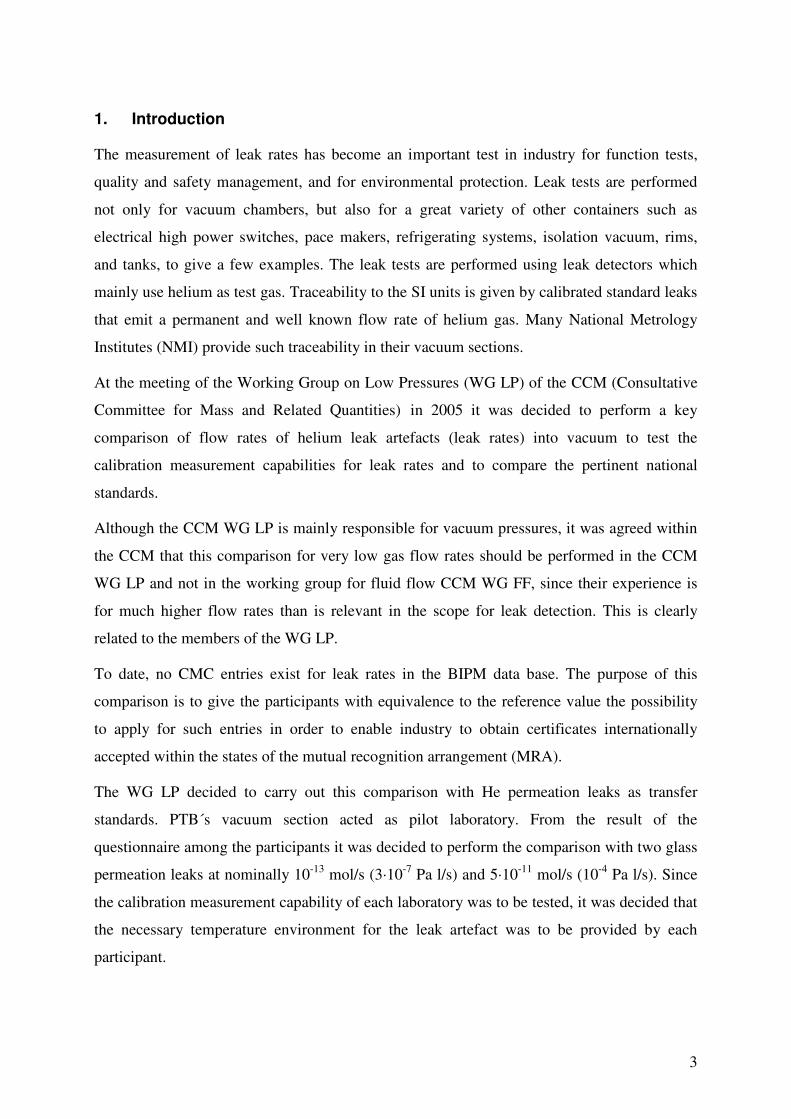
Quantitative leak tests with vacuum technology have become an important tool in industry for safety and operational reasons and to meet environmental regulations. In lack of a relevant key comparison, so far, there are no calibration measurement capabilities published in the BIPM data base. To enable national metrology institutes providing service for leak rate calibrations to apply for these entries in the data base and to ensure international equivalence in this field, key comparison CCM.P-K12 was organised. The goal of this comparison was to compare the national calibration standards and procedures for helium leak rates. Two helium permeation leak elements of 4⋅10-11 mol/s (L1) and 8⋅10-14 mol/s (L2) served as transfer standards and were measured by 11 national metrology institutes for L1 and 6 national metrology institutes for L2. Equivalence could be shown for 8 laboratories in the case of L1 and for all 6 in the case of L2. Three different evaluation methods were applied and are presented in this report, but the random effects model was accepted as most suitable in our case.

2

Content

1. INTRODUCTION ....................................................................................................................................... 3

2. TRANSFER STANDARDS AND QUANTITY TO BE DETERMINED ............................................... 4

3. PARTICIPATING LABORATORIES AND THEIR MEASUREMENT SYSTEMS .......................... 4

3.1. CMI ...................................................................................................................................................... 6

3.2. IMT ...................................................................................................................................................... 7

3.3. INRIM .................................................................................................................................................. 8

3.4. LNE ...................................................................................................................................................... 8

3.5. NIM ...................................................................................................................................................... 9

3.6. NIST ................................................................................................................................................... 10

3.7. NMC-A*STAR .................................................................................................................................. 11

3.8. NMIJ .................................................................................................................................................. 11

3.9. NPL/I ................................................................................................................................................. 11

3.10. PTB .................................................................................................................................................... 12

3.11. VNIIM ............................................................................................................................................... 12

4. CHRONOLOGY AND MEASUREMENT PROCEDURE ................................................................... 13

5. UNCERTAINTIES OF REFERENCE STANDARDS ........................................................................... 14

6. PROBLEMS WITH THE TRANSFER STANDARDS ......................................................................... 15

7. RESULTS OF THE PILOT LABORATORY ........................................................................................ 16

7.1. TEMPERATURE COEFFICIENT OF TRANSFER STANDARD LEAKS ............................................................ 16

7.2. RESULTS OF THE PILOT LABORATORY ................................................................................................. 17

7.3. TIME-DEPENDENT BEHAVIOUR OF TRANSFER STANDARDS .................................................................. 20

8. REPORTED RESULTS OF EACH LABORATORY ........................................................................... 20

8.1. TRANSFER LEAK ARTEFACT L1 ........................................................................................................... 20

8.2. TRANSFER LEAK ARTEFACT L2 ........................................................................................................... 23

9. CALCULATION OF REFERENCE VALUE AND DEGREE OF EQUIVALENCE ........................ 25

9.1. GENERAL CONSIDERATIONS ................................................................................................................ 25

9.2. EVALUATION METHOD AND RESULTS .................................................................................................. 27

10. DEGREES OF EQUIVALENCE OF PAIRS OF NATIONAL MEASUREMENT STANDARDS ... 32

11. DISCUSSION AND CONCLUSIONS ..................................................................................................... 32

12. REFERENCES .......................................................................................................................................... 34

13. APPENDIX ................................................................................................................................................ 35

13.1. ALTERNATIVE EVALUATION METHOD BY ZHANG ET AL. ..................................................................... 35

13.2. CALCULATION OF DEGREES OF EQUIVALENCE BY BAYESIAN MODEL AVERAGING (FIXED EFFECT

MODEL) 39

13.3. CODE FOR RANDOM EFFECTS MODEL .................................................................................................. 46

13.4. TABLES OF PAIR-WISE DIFFERENCES (RANDOM EFFECTS MODEL)........................................................ 48

3

1. Introduction

The measurement of leak rates has become an important test in industry for function tests,

quality and safety management, and for environmental protection. Leak tests are performed

not only for vacuum chambers, but also for a great variety of other containers such as

electrical high power switches, pace makers, refrigerating systems, isolation vacuum, rims,

and tanks, to give a few examples. The leak tests are performed using leak detectors which

mainly use helium as test gas. Traceability to the SI units is given by calibrated standard leaks

that emit a permanent and well known flow rate of helium gas. Many National Metrology

Institutes (NMI) provide such traceability in their vacuum sections.

At the meeting of the Working Group on Low Pressures (WG LP) of the CCM (Consultative

Committee for Mass and Related Quantities) in 2005 it was decided to perform a key

comparison of flow rates of helium leak artefacts (leak rates) into vacuum to test the

calibration measurement capabilities for leak rates and to compare the pertinent national

standards.

Although the CCM WG LP is mainly responsible for vacuum pressures, it was agreed within

the CCM that this comparison for very low gas flow rates should be performed in the CCM

WG LP and not in the working group for fluid flow CCM WG FF, since their experience is

for much higher flow rates than is relevant in the scope for leak detection. This is clearly

related to the members of the WG LP.

To date, no CMC entries exist for leak rates in the BIPM data base. The purpose of this

comparison is to give the participants with equivalence to the reference value the possibility

to apply for such entries in order to enable industry to obtain certificates internationally

accepted within the states of the mutual recognition arrangement (MRA).

The WG LP decided to carry out this comparison with He permeation leaks as transfer

standards. PTB´s vacuum section acted as pilot laboratory. From the result of the

questionnaire among the participants it was decided to perform the comparison with two glass

permeation leaks at nominally 10-13 mol/s (3·10-7 Pa l/s) and 5·10-11 mol/s (10-4 Pa l/s). Since

the calibration measurement capability of each laboratory was to be tested, it was decided that

the necessary temperature environment for the leak artefact was to be provided by each

participant.

4

2. Transfer standards and quantity to be determined

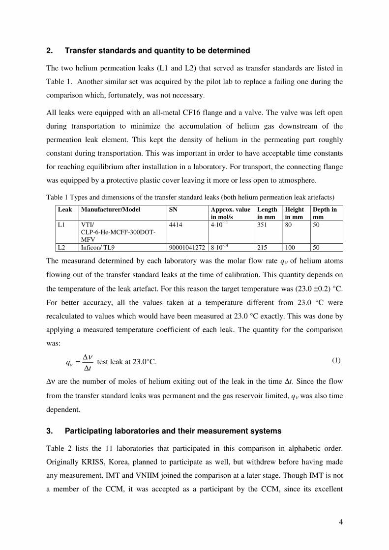
The two helium permeation leaks (L1 and L2) that served as transfer standards are listed in

Table 1. Another similar set was acquired by the pilot lab to replace a failing one during the

comparison which, fortunately, was not necessary.

All leaks were equipped with an all-metal CF16 flange and a valve. The valve was left open

during transportation to minimize the accumulation of helium gas downstream of the

permeation leak element. This kept the density of helium in the permeating part roughly

constant during transportation. This was important in order to have acceptable time constants

for reaching equilibrium after installation in a laboratory. For transport, the connecting flange

was equipped by a protective plastic cover leaving it more or less open to atmosphere.

Table 1 Types and dimensions of the transfer standard leaks (both helium permeation leak artefacts)

Leak Manufacturer/Model SN Approx. value

in mol/s

Length

in mm

Height

in mm

Depth in

mm

L1 VTI/ CLP-6-He-MCFF-300DOT-MFV

4414 4·10-11 351 80 50

L2 Inficon/ TL9 90001041272 8·10-14 215 100 50

The measurand determined by each laboratory was the molar flow rate qν of helium atoms

flowing out of the transfer standard leaks at the time of calibration. This quantity depends on

the temperature of the leak artefact. For this reason the target temperature was (23.0 ±0.2) °C.

For better accuracy, all the values taken at a temperature different from 23.0 °C were

recalculated to values which would have been measured at 23.0 °C exactly. This was done by

applying a measured temperature coefficient of each leak. The quantity for the comparison

was:

test leak at 23.0°C. (1)

∆ν are the number of moles of helium exiting out of the leak in the time ∆t. Since the flow

from the transfer standard leaks was permanent and the gas reservoir limited, qν was also time

dependent.

3. Participating laboratories and their measurement systems

Table 2 lists the 11 laboratories that participated in this comparison in alphabetic order.

Originally KRISS, Korea, planned to participate as well, but withdrew before having made

any measurement. IMT and VNIIM joined the comparison at a later stage. Though IMT is not

a member of the CCM, it was accepted as a participant by the CCM, since its excellent

tq

∆

∆=

νν

5

measurement capabilities for leaks and outgassing rates are well known and were regarded as

highly beneficial to the comparison.

In the second column of Table 2, the standards used for the calibration of the transfer

standards are listed. The third column gives the method, and the last column lists whether the

standard is independent or is traceable to another NMI. All standards were considered as

primary [1].

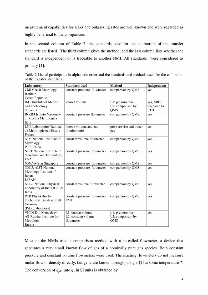
Table 2 List of participants in alphabetic order and the standards and methods used for the calibration of the transfer standards.

Laboratory Standard used Method Independent

CMI Czech Metrology Institute Czech Republic

constant pressure flowmeter comparison by QMS yes

IMT Institute of Metals and Technology Slovenia

known volume L1: pressure rise L2: comparison by QMS

yes, SRG traceable to PTB

INRIM Istituto Nazionale di Ricerca Metrologica Italy


LNE Laboratoire National de Métrologie et d'Essais France

known volume and gas dilution ratio

pressure rise and tracer gas

yes

NIM National Institute of Metrology P. R. China

constant volume flowmeter comparison by QMS yes

NIST National Institute of Standards and Technology USA


NMC-A*star Singapore constant pressure flowmeter comparison by QMS yes NMIJ, AIST National Metrology Institute of Japan JAPAN


NPL/I National Physical Laboratory of India (CSIR) India

constant volume flowmeter comparison by QMS yes

PTB Physikalisch-Technische Bundesanstalt Germany (Pilot Laboratory)

constant pressure flowmeter FM1

comparison by QMS yes

VNIIM D.I. Mendeleev All-Russian Institute for Metrology Russia

L1: known volume L2: constant volume flowmeter

L1: pressure rise L2: comparison by QMS

yes

Most of the NMIs used a comparison method with a so-called flowmeter, a device that

generates a very small known flow of gas of a nominally pure gas species. Both constant

pressure and constant volume flowmeters were used. The existing flowmeters do not measure

molar flow or density directly, but generate known throughputs qpV [2] at some temperature T.

The conversion of qpV into qν in SI units is obtained by

6

RT

qq

pV=ν , (2)

R =8.3145 Pa m³ mol-1 K

-1 being the universal gas constant.

In three cases, the molar flow rate was determined by measuring the pressure rise due to the

leak or a secondary standard (gas mixture delivered by a capillary used as auxiliary device,

LNE) into a known volume and converting the measured qpV =V∆p/∆t as described by

equation (2).

3.1. CMI

The CMI used a comparison method with a constant pressure flowmeter. A quadrupole mass

spectrometer (QMS, Balzers Prisma) installed at the calibration chamber of a continuous

expansion system [3] to [7] served as indicator to compare the helium gas flows from the flow

meter (signal on QMS: I2) and from the transfer standard leak (signal on QMS: I1), which

were intermittently admitted into the calibration chamber. The calibrated leak was connected

to an auxiliary turbomolecular pump (backed by a membrane pump) in the periods when it

was not connected to the calibration chamber. The linearity of the QMS was checked in the

relevant range of this comparison. The non-linearity was found to be insignificant.

Nevertheless the gas flow from the flowmeter was set by the sapphire valve so to give a

partial pressure signal as close as possible to the signal caused by the transfer standard. The

signal drift of the QMS was fitted by a cubic polynomial function with time. The molar flow

rate from the leak under calibration is given by

, (3)

where I1,2 are offset corrected readings. The offset reading is obtained when there is no helium

flow onto the QMS.

No thermal bath was utilised to stabilize the temperature of the transfer standards. Instead,

they were thermally insulated by the means of a foam wrap. Its temperature was measured by

three sensors fixed to its reservoir container and the mean of their indications was taken into

account. The temperature of the transfer standard remained stable within approximately 0.1

°C.

It should be noted that after the measurements the CMI discovered an air leak in the valve

used to close the connection to the transfer leak element. In some cases the presence of the

other gases, particularly water vapour, caused changes in the sensitivity of the QMS for

helium. This may have contributed to an error of the measurement results. The effect of this

12

1FM,

2

1leak, ≈=

I

Iq

I

Iq νν

7

air leak, however, was not reproducible enough to conclude that an error in the QMS reading

had occurred with a reasonable degree of probability. Therefore the CMI results were not

removed from the comparison.

3.2. IMT

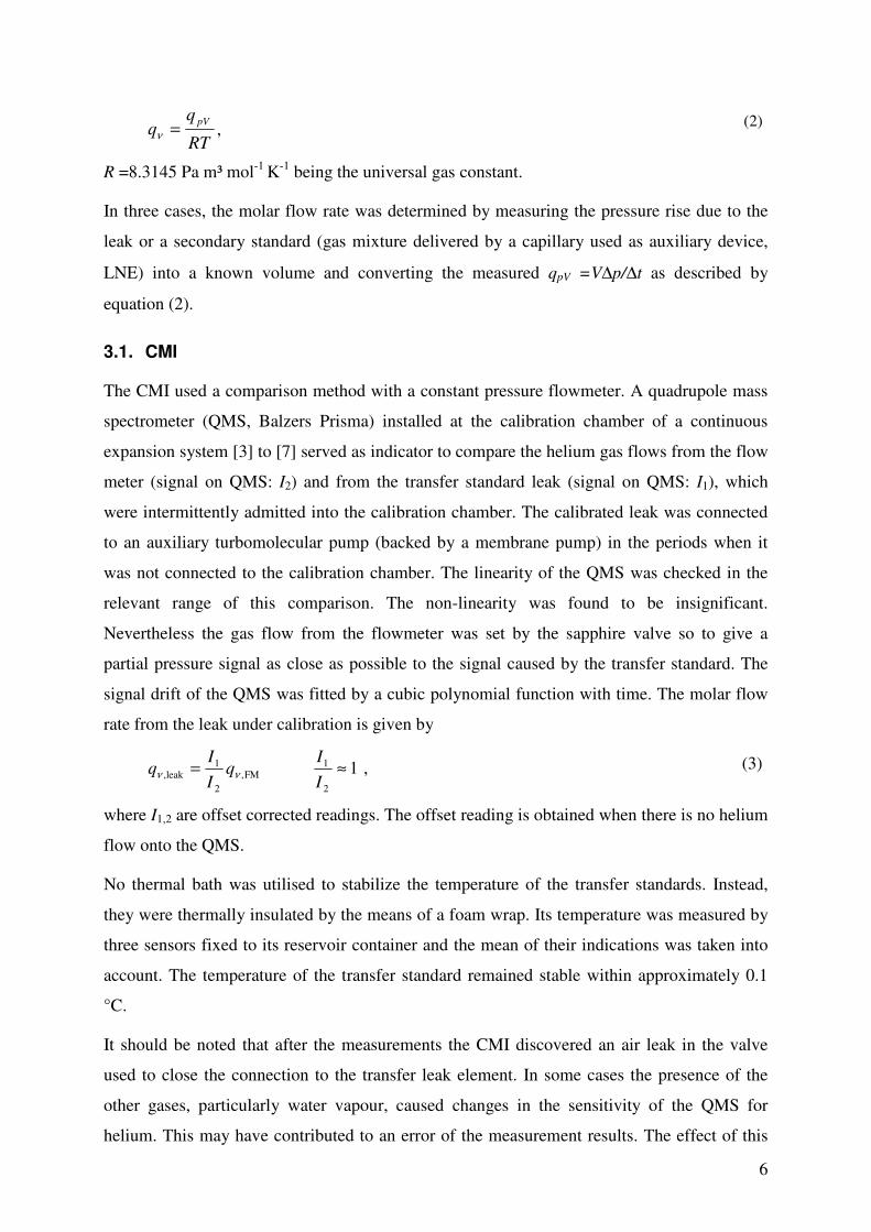
The IMT has developed a primary helium leak [8] based on a glass permeation element, a

reservoir with adjustable helium gas pressure and a calibration facility for in-situ

measurement of generated helium gas flow by a pressure rise method using spinning rotor

gauge (Figure 1). The fill pressure in the reservoir can be varied from 100 Pa to 1 MPa, to

generate flows from 10-15 mol/s to 10-11 mol/s with the glass permeation element at room

temperature.

Figure 1 The IMT leak calibration/comparison system

Compared to the description in [8] some improvements were made, e.g. a temperature shroud

made of Al with a possibility to heat the helium reservoir with the glass permeation element

to 140 °C, Ti/Ta getter was replaced with ST 122 NEG from SAES Getters.

This primary helium leak is connected to a leak comparator apparatus shown in Figure 1. The

He partial pressure in the comparator vacuum chamber (CH2) is measured with a quadrupole

UUT

IMT primaryreference leak

NEG

ORIFICE

TURBO

SRG 1

CH1

He

CH2SRG 2

BAG

QMS1

QMS2

8

mass spectrometer (QMS1). The He gas pressure in the reservoir of the primary leak is

preliminary adjusted to produce nearly the same He signal as the unit under test (UUT).

The volume of the comparator vacuum chamber was also determined. This enables direct

primary measurement of He gas flow from UUT by pressure rise method in CH2 (nominal

volume 7 L) using SRG 2. This method is generally used for He flows from 10-13 mol/s to

3·10-9 mol/s.

The purity of accumulated helium gas can be checked by another quadrupole mass

spectrometer (QMS2).

The transfer standard L1 was determined by measuring the helium pressure increase in CH2

using SRG2 while L2 was measured by comparison with the IMT primary leak using QMS1.

The direct measurement of helium gas flow from L2 was not possible, because an additional

air leak in the transfer leak artefact itself (see also Section 6). The argon gas from this air leak

was also accumulated in CH2 in addition to helium (NEG pump attached to CH2 pumps all

atmospheric gases except Ar).

3.3. INRIM

The INRIM used a comparison method with a flowmeter similar to the one described for the

CMI. The flowmeter F3 was described in [9]. The temperature of the laboratory is regulated

to (23.0 ± 0.1) °C by an automatic and active control. The temperature associated to the

permeation leak has been controlled using a water thermostatic bath, in order to regulate the

temperature at 23 °C, with a deviation less than 0.1 °C.

3.4. LNE

The LNE applied a two-step procedure. In a first step, the throughput of a reference capillary

was calibrated in dependence of upstream nitrogen pressure p (150 kPa to 700 kPa) by a

pressure rise method. The throughput (qpV)N2 of nitrogen at temperature Tc was then fitted by

the second order polynomial

. (4)

The residuals from this fitting polynomial were less than 0.05% of (qpV)N2.

In a second step, the upstream nitrogen gas was mixed with a known and small relative

amount c of helium (tracer gas) such that the signal I2 from the downstream side of the

capillary on a mass spectrometer type leak detector was approximately identical to the signal

( ) 2210N2

pmpmmq pV ++=

9

I1 generated by the leak artefact under calibration at temperature Tm. The helium throughput

(qpV)He of the leak artefact is then given by

( ) ( ) ( ) 01212c

m

N2He≈−−−= IIIIS

T

Tcqq pVpV ,

(5)

where S is the sensitivity of the leak detector. To obtain the molar flow rate, (qpV)He is divided

by RTm.

The Type B uncertainties of this procedure are estimated to 1.3% (L1) and 1.4% (L2), where

the main contribution comes from the calibration of the capillary by the pressure rise method.

To control the temperature of the transfer leaks, a thermo regulated bath filled with water and

equipped with an external circulator was used. A silicon tubing of 7 mm inner diameter,

connected to the external circulation of the bath, surrounds the leak and regulates its

temperature to 23 °C. A calibrated Pt100 sensor was attached to the reservoir of the transfer

leak. The leak’s temperature was assumed to be the Pt100 sensor’s temperature. The

instability of temperature (given by standard deviation of the mean) measured with the sensor

was lower than 5 mK over 30 minutes.

3.5. NIM

The NIM used a comparison with a constant volume flowmeter. The pressure decrease ∆p of

the known volume V in the flowmeter in time period ∆t was measured by a CDG with a

fullscale of 1.33 kPa calibrated at NIM. By means of a flow divider the flow from the

flowmeter could be reduced by the factor 0.006. A quadrupole mass spectrometer installed at

a larger chamber behind the flow divider served as indicator to compare the gas flows from

the flow meter and from the transfer standard attached to the same chamber.

−

∆

−= ∑

=

+0

1

1

2

11Q

t

PPV

I

I

nRT

kq

n

i

ii

ν , (6)

where the offset corrected signals on the QMS I1 and I2 are denoted as above and Q0 is the

background signal from the flowmeter.

The temperature was adjusted by the air conditioning of the room. Two Pt100 sensors were

used to measure temperature of the leak artefact which was enclosed in foam material. During

the leak rate measurement the air conditioning was switched off.

10

3.6. NIST

The NIST primary leak standard (PLS) utilizes a comparison method with a flowmeter similar

as that described for the CMI. The PLS consists of a constant pressure flowmeter [10] that

produces a low gas flow into a continuous expansion chamber. The continuous expansion

chamber is divided into an upper and lower chamber by a small orifice; a QMS is mounted

onto the upper chamber and a turbomolecular pump is connected to the lower chamber. For

L1, the He flow from L1 was compared to that from the flowmeter by alternately flowing He

from L1 and the flowmeter into the upper chamber of the expansion chamber, comparing the

QMS signals of each, and applying Eq. (3). The flow rate of L2 was measured by a flow

division technique that extends the lower limit of the PLS to 2·10-14 mol/s. By using the

flowmeter to alternatively produce helium flows qν,upper into the upper chamber and qν,lower

into the lower chamber, which produce the same partial pressure of He in the upper chamber,

a flow ratio between the two chambers was measured:

.

(7)

r was approximately equal to 170. This ratio was measured ten times and the average value

was used in the analysis. Helium flow from L2 was directed into the upper vacuum chamber,

where it subsequently flowed through the orifice and was evacuated by the pump. After the

gas flow and the upper chamber pressure reached equilibrium (20 minutes), the quadrupole

mass spectrometer signal was recorded (as was done for L1). The leak artefact was then

isolated from the main vacuum chamber and He flow from the bellows flowmeter was

directed into the lower chamber. The gas flow from the flowmeter was adjusted so that the

partial pressure of helium in the upper chamber was the same as that recorded when flow

from L2 was directed into the upper chamber. The unknown flow rate from the leak artefact is

then determined from

, (8)

where I1,2 are offset corrected readings. The offset reading was obtained when there was no

helium flow into the system.

The He leak artefact was placed in a temperature controlled box which was insulated from the

laboratory atmosphere. The temperature within the box was controlled to better than 20 mK.

The temperature of the He leak artefact was measured by a calibrated PRT strapped to the

body of the leak artefact.

upper,

lower,

ν

ν

q

qr =

12

1FM,

2

1leak, ≈=

I

Irq

I

Iq νν

11

3.7. NMC-A*STAR

NMC-A*STAR (formerly SPRING) used a comparison method with a primary flowmeter

[11]. The outlet flow rate is given by:

)/()/()/(/2

tTTR

Vptp

TR

VtV

TR

ptN i ∆∆⋅

⋅

⋅−∆∆⋅

⋅+∆∆⋅

⋅=∆∆ , (9)

where: ∆t is the time interval of flow rate measurement; ∆p is the drop pressure in flow meter;

∆V is the piston displacement volume and ∆T the temperature change of the volume V in the

measured time interval.

The chamber for comparison was built similar as one of a continuous expansion chamber.

NMC-A*STAR calibrated the reading of the QMS for qν by varying the helium flow rates qν

from the flow meter around the expected value of the leak. A straight line was fitted to the

data I2(qν). In such a way for each measured I1 a corresponding qν was determined.

The calibration was conducted under the laboratory temperature condition of (23 ±0.5) oC.

The standard leak was placed into a thermal insulated case for stabilising temperature. A

calibrated Pt100 resistor was used to measure the temperature of L1.

3.8. NMIJ

The NMIJ used a comparison method with a flowmeter. The flowmeter is a constant pressure

type with a metal capillary (inner diameter: 0.15 mm, length: 15 mm) as a flow rate restrictor.

Helium gas flows, ranging from 4⋅10-9 Pa m3/s to 8⋅10-4 Pa m3/s, are generated by the change

of the pressure in the flowmeter from 0.16 Pa to 5000 Pa [12]. The flowmeter temperature

was at (23.0 ± 0.2) ˚C. The transfer standard leak was set in a self-remodeled refrigerator for

stabilizing its temperature. The temperature of the leak was measured by a calibrated platinum

resistance thermometer (PRT). The dynamic flow system was used as a calibration apparatus

for the leak. A QMS was used as a comparator for evaluating the flow rate.

3.9. NPL/I

The NPL/I used a comparison method with a flowmeter similar as described for the NIST in

the Section 3.6 except that a constant volume flowmeter was used. Details of the NPL/I

standard are given in [13] to [16]. As for NIST, the flow rate from L2 had to be measured by

applying a flow division in the continuous expansion standard. The flow ratio of the upper

12

and lower chamber (Eq. (7)) depends on the gas species and was determined to be equal to 18

for helium.

Three years after completion of the measurements NPL/I found that the value of the volume

used for the constant flow volume flowmeter was too high by 1.44%. This also caused the

leak rate values reported for L1 and L2 to be high by 1.44%. Since Draft A had been

approved for a long time already, this individual error could not be corrected.

The flowmeter, the chambers and the leak artefact were enclosed in a black foam enclosure

for temperature stabilization. The temperature of the different parts were determined by 5

PRTs, one of them was attached to the transfer leak under comparison. The temperature of the

laboratory was stablized to within ± 0.5 °C by means of air conditioners.

3.10. PTB

Also PTB used a comparison method with a flowmeter. The signal I1 on a quadrupole mass

spectrometer generated by the helium flow from the leak artefact was compared to the signal

I2 generated by the known molar flow rate qν,FM of helium from the flowmeter. The

quadrupole mass spectrometer (QMS) was far away from both the leak artefact and the

flowmeter. This ensured that the flow conditions and the temperatures of the helium atoms at

the location of the QMS were the same in the two cases.

The molar flow rate from the leak under calibration is given by Eq. (3).

The flowmeter used was described in [17]. It was modernized, however, since then, mainly

for automated data recording. For measurement of L1 the flowmeter was operated in the

constant pressure mode, for L2 in the constant conductance mode.

The standard leaks were immersed in a temperature controlled water bath to stabilize their

temperature. Calibrated Pt100 resistors were used to measure the temperatures of L1 and L2.

3.11. VNIIM

The VNIIM used a pressure rise method for L1 and a comparison by means of a QMS with a

constant volume flowmeter for L2.

To measure the leak rate of L1 by measuring the pressure increase in a constant volume the

following equation was used:

Vtt

p

tt

pq pV ⋅

−′′

′′∆−

−′

′∆= )(

00

, (10)

13

where ∆p´ and ∆p´´ are pressure increments in the chamber with volume V caused by the

flow to be measured and by the flow from other processes (e.g, desorption) in time intervals

t´-t0 and t´´-t0.

The chamber volume of about 140 cm³ was determined by the gravimetric method. The value

of pressure change in the known volume was determined by means of a standard being part of

the national standard of low absolute pressures.

For leak L2 a comparative method by means of QMS was used. The measurement equation is

similar to Eq. (3).

Temperature control of the leaks was obtained by using a liquid thermostat with a

stabilization of the temperature not exceeding 0.1 ºС, and the maximum permissible error of

setting the reference temperature not exceeding 0.2 ºС.

4. Chronology and measurement procedure

In order to determine the time dependence of the quantity qν, it was decided that after three

participants the leak artefacts were to be returned to the pilot laboratory for re-calibration.

Each laboratory measured the flow rate from L1, but for 5 of the participants the lower flow

rate of L2 was out of their measurement scope and not measured.

Significant delays occurred between NIM and NMC-A*STAR due to a lost ATA Carnet, and

also between NMIJ and VNIIM due to a customs problem. For these reasons and,

additionally, because IMT and VNIIM joined at a later stage, the total measurement time

extended to 25 months instead of the originally planned 17 months.

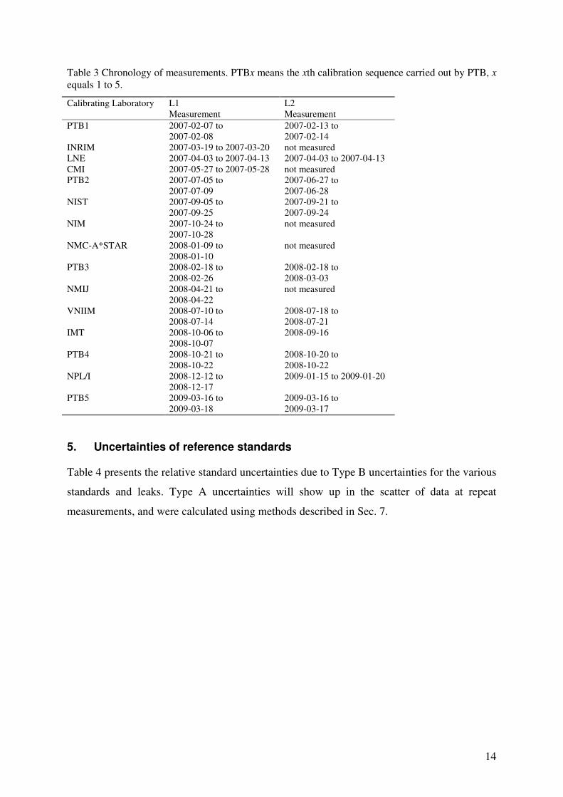
Table 3 presents the actual chronology of the calibrations.

Each laboratory was required to perform 7 measurements on a single calibration day and to

repeat this series on another day. If supplied, additional measurements were accepted.

IMT performed the two measurement series for L2 on a single day. The NMC-A*STAR

laboratory could only complete one calibration day with 5 measurements.

14

Table 3 Chronology of measurements. PTBx means the xth calibration sequence carried out by PTB, x equals 1 to 5.

Calibrating Laboratory L1 Measurement

L2 Measurement

PTB1 2007-02-07 to 2007-02-08

2007-02-13 to 2007-02-14

INRIM 2007-03-19 to 2007-03-20 not measured LNE 2007-04-03 to 2007-04-13 2007-04-03 to 2007-04-13 CMI 2007-05-27 to 2007-05-28 not measured PTB2 2007-07-05 to

2007-07-09 2007-06-27 to 2007-06-28

NIST 2007-09-05 to 2007-09-25

2007-09-21 to 2007-09-24

NIM 2007-10-24 to 2007-10-28

not measured

NMC-A*STAR 2008-01-09 to 2008-01-10

not measured

PTB3 2008-02-18 to 2008-02-26

2008-02-18 to 2008-03-03

NMIJ 2008-04-21 to 2008-04-22

not measured

VNIIM 2008-07-10 to 2008-07-14

2008-07-18 to 2008-07-21

IMT 2008-10-06 to 2008-10-07

2008-09-16

PTB4 2008-10-21 to 2008-10-22

2008-10-20 to 2008-10-22

NPL/I 2008-12-12 to 2008-12-17

2009-01-15 to 2009-01-20

PTB5 2009-03-16 to 2009-03-18

2009-03-16 to 2009-03-17

5. Uncertainties of reference standards

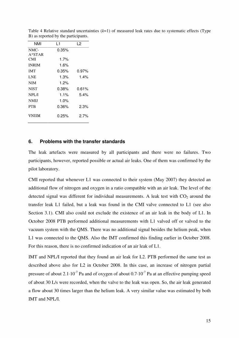
Table 4 presents the relative standard uncertainties due to Type B uncertainties for the various

standards and leaks. Type A uncertainties will show up in the scatter of data at repeat

measurements, and were calculated using methods described in Sec. 7.

15

Table 4 Relative standard uncertainties (k=1) of measured leak rates due to systematic effects (Type B) as reported by the participants.

NMI L1 L2

NMC-A*STAR

0.35%

CMI 1.7%

INRIM 1.6%

IMT 0.35% 0.97%

LNE 1.3% 1.4%

NIM 1.2%

NIST 0.38% 0.61%

NPL/I 1.1% 5.4%

NMIJ 1.0%

PTB

0.36%

2.3%

VNIIM 0.25% 2.7%

6. Problems with the transfer standards

The leak artefacts were measured by all participants and there were no failures. Two

participants, however, reported possible or actual air leaks. One of them was confirmed by the

pilot laboratory.

CMI reported that whenever L1 was connected to their system (May 2007) they detected an

additional flow of nitrogen and oxygen in a ratio compatible with an air leak. The level of the

detected signal was different for individual measurements. A leak test with CO2 around the

transfer leak L1 failed, but a leak was found in the CMI valve connected to L1 (see also

Section 3.1). CMI also could not exclude the existence of an air leak in the body of L1. In

October 2008 PTB performed additional measurements with L1 valved off or valved to the

vacuum system with the QMS. There was no additional signal besides the helium peak, when

L1 was connected to the QMS. Also the IMT confirmed this finding earlier in October 2008.

For this reason, there is no confirmed indication of an air leak of L1.

IMT and NPL/I reported that they found an air leak for L2. PTB performed the same test as

described above also for L2 in October 2008. In this case, an increase of nitrogen partial

pressure of about 2.1⋅10-7 Pa and of oxygen of about 0.7⋅10-7 Pa at an effective pumping speed

of about 30 L/s were recorded, when the valve to the leak was open. So, the air leak generated

a flow about 30 times larger than the helium leak. A very similar value was estimated by both

IMT and NPL/I.

16

This apparent air leak from L2 would have affected measurements where the measurement

apparatus was not only sensitive to helium, but also to other gases or to a total pressure rise.

The only laboratory that normally performed the measurement in such a way (IMT for L2)

was aware of the leak and changed the measurement method accordingly.

There may also be an effect in cases where the helium sensitivity of a QMS changes

significantly with the presence of other gases. This is known to happen for pressures higher

than 10-4 Pa, but rarely below. Since the pressure rise from the air leak was relative modest

and normally below 10-6 Pa (depending on the pumping speed), it is a rather improbable

scenario, however.

The flow division technique applied by NIST and NPL/I would be affected, if a total pressure

gauge instead of a QMS would be used or the helium flow and the respective flow ratio would

be changed by the additional air flow. Since the total pressures as described above remained

in the high vacuum range, the interaction between different gas molecules is so rare (if this

would not be the case, the flow division is difficult to apply), that a disturbance can be

excluded as well.

In conclusion, any significant falsification of results by the transfer standards in any lab can

be excluded. It should be noted that calibration measurement capabilities of helium test leaks

were tested by this comparison. This means that the measurement procedure should be

specific to the helium flow from the leak artefact and not measure the total flow from it.

7. Results of the pilot laboratory

7.1. Temperature coefficient of transfer standard leaks

To correct the data obtained at different temperatures to a common reference temperature, the

temperature coefficients of the flow rate from the leak artefacts had to be determined. The

temperature was varied from 291 K (L2) or 292 K (L1) up to 304 K and the flow rate

measured at several temperatures after stabilization.

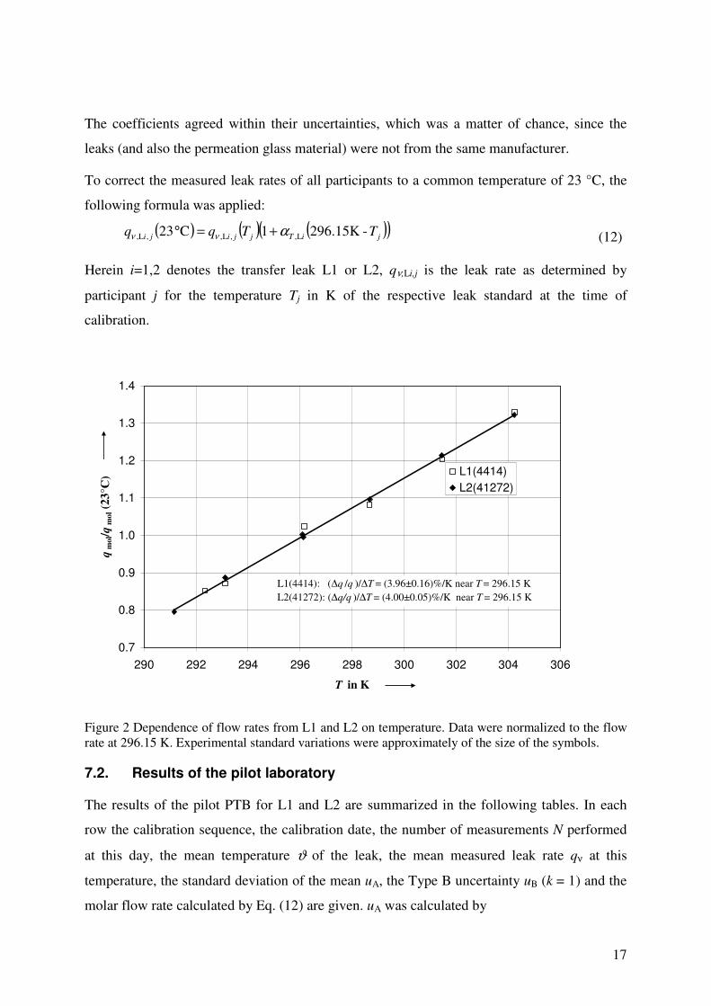
The results for both leaks are shown on Figure 2. The flow rate data from the leaks were

normalized to their respective values at 23°C. A linear least square fit was applied to the data

of both leaks to determine the slopes as relative temperature coefficients αT of the flow rates:

( )( ) 1-

l

L1,L1, K%16.096.3

C23: ±=

∆°

∆=

Tq

qT

ν

να (11)

( )( ) 1-

l

L2,L2, K%05.000.4

C23: ±=

∆°

∆=

Tq

qT

ν

να

17

The coefficients agreed within their uncertainties, which was a matter of chance, since the

leaks (and also the permeation glass material) were not from the same manufacturer.

To correct the measured leak rates of all participants to a common temperature of 23 °C, the

following formula was applied:

( ) ( ) ( )( )jiTjjiji TTqq -K15.2961C23 L,,L,,L, ανν +=° (12)

Herein i=1,2 denotes the transfer leak L1 or L2, qν,Li,j is the leak rate as determined by

participant j for the temperature Tj in K of the respective leak standard at the time of

calibration.

Figure 2 Dependence of flow rates from L1 and L2 on temperature. Data were normalized to the flow rate at 296.15 K. Experimental standard variations were approximately of the size of the symbols.

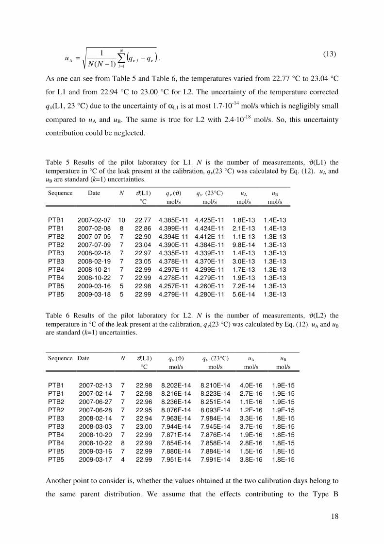
7.2. Results of the pilot laboratory

The results of the pilot PTB for L1 and L2 are summarized in the following tables. In each

row the calibration sequence, the calibration date, the number of measurements N performed

at this day, the mean temperature ϑ of the leak, the mean measured leak rate qν at this

temperature, the standard deviation of the mean uA, the Type B uncertainty uB (k = 1) and the

molar flow rate calculated by Eq. (12) are given. uA was calculated by

0.7

0.8

0.9

1.0

1.1

1.2

1.3

1.4

290 292 294 296 298 300 302 304 306

T in K

qm

ol/q

mo

l (23

°C) L1(4414)

L2(41272)

L1(4414): (∆q /q )/∆T = (3.96±0.16)%/K near T = 296.15 KL2(41272): (∆q/q )/∆T = (4.00±0.05)%/K near T = 296.15 K

18

( )∑=

−−

=N

l

l qqNN

u1

,A )1(

1νν . (13)

As one can see from Table 5 and Table 6, the temperatures varied from 22.77 °C to 23.04 °C

for L1 and from 22.94 °C to 23.00 °C for L2. The uncertainty of the temperature corrected

qν(L1, 23 °C) due to the uncertainty of αL1 is at most 1.7·10-14 mol/s which is negligibly small

compared to uA and uB. The same is true for L2 with 2.4·10-18 mol/s. So, this uncertainty

contribution could be neglected.

Table 5 Results of the pilot laboratory for L1. N is the number of measurements, ϑ(L1) the temperature in °C of the leak present at the calibration, qν(23 °C) was calculated by Eq. (12). uA and uB are standard (k=1) uncertainties.

Sequence Date N ϑ(L1) qν (ϑ) qν (23°C) uA uB

°C mol/s mol/s mol/s mol/s

PTB1 2007-02-07 10 22.77 4.385E-11 4.425E-11 1.8E-13 1.4E-13

PTB1 2007-02-08 8 22.86 4.399E-11 4.424E-11 2.1E-13 1.4E-13

PTB2 2007-07-05 7 22.90 4.394E-11 4.412E-11 1.1E-13 1.3E-13

PTB2 2007-07-09 7 23.04 4.390E-11 4.384E-11 9.8E-14 1.3E-13

PTB3 2008-02-18 7 22.97 4.335E-11 4.339E-11 1.4E-13 1.3E-13

PTB3 2008-02-19 7 23.05 4.378E-11 4.370E-11 3.0E-13 1.3E-13

PTB4 2008-10-21 7 22.99 4.297E-11 4.299E-11 1.7E-13 1.3E-13

PTB4 2008-10-22 7 22.99 4.278E-11 4.279E-11 1.9E-13 1.3E-13

PTB5 2009-03-16 5 22.98 4.257E-11 4.260E-11 7.2E-14 1.3E-13

PTB5 2009-03-18 5 22.99 4.279E-11 4.280E-11 5.6E-14 1.3E-13

Table 6 Results of the pilot laboratory for L2. N is the number of measurements, ϑ(L2) the temperature in °C of the leak present at the calibration, qν(23 °C) was calculated by Eq. (12). uA and uB are standard (k=1) uncertainties.

Sequence Date N ϑ(L1) qν (ϑ) qν (23°C) uA uB

°C mol/s mol/s mol/s mol/s

PTB1 2007-02-13 7 22.98 8.202E-14 8.210E-14 4.0E-16 1.9E-15

PTB1 2007-02-14 7 22.98 8.216E-14 8.223E-14 2.7E-16 1.9E-15

PTB2 2007-06-27 7 22.96 8.236E-14 8.251E-14 1.1E-16 1.9E-15

PTB2 2007-06-28 7 22.95 8.076E-14 8.093E-14 1.2E-16 1.9E-15

PTB3 2008-02-14 7 22.94 7.963E-14 7.984E-14 3.3E-16 1.8E-15

PTB3 2008-03-03 7 23.00 7.944E-14 7.945E-14 3.7E-16 1.8E-15

PTB4 2008-10-20 7 22.99 7.871E-14 7.876E-14 1.9E-16 1.8E-15

PTB4 2008-10-22 8 22.99 7.854E-14 7.858E-14 2.8E-16 1.8E-15

PTB5 2009-03-16 7 22.99 7.880E-14 7.884E-14 1.5E-16 1.8E-15

PTB5 2009-03-17 4 22.99 7.951E-14 7.991E-14 3.8E-16 1.8E-15

Another point to consider is, whether the values obtained at the two calibration days belong to

the same parent distribution. We assume that the effects contributing to the Type B

19

uncertainties are no different at (more or less) successive calibrations days within the same

sequence. Therefore we consider the values measured on different days to be compatible, if

the absolute difference between the mean values is smaller than two standard deviations of the

difference:

. (14)

Herein qν,1 and qν,2 are the mean values determined on their respective calibration days with

uA,1, uA,2 being their respective sample standard deviations.

From Table 5 and Table 6 one can calculate that, with the exception of PTB5 for L1 and

PTB2 for L2, the mean values on different days in a sequence agreed within two standard

deviations of the difference, and most agreed to well within one.

If they agree, the mean and standard deviation of the mean of all the data at the two

measurement days within each calibration sequence can be taken for further evaluation.

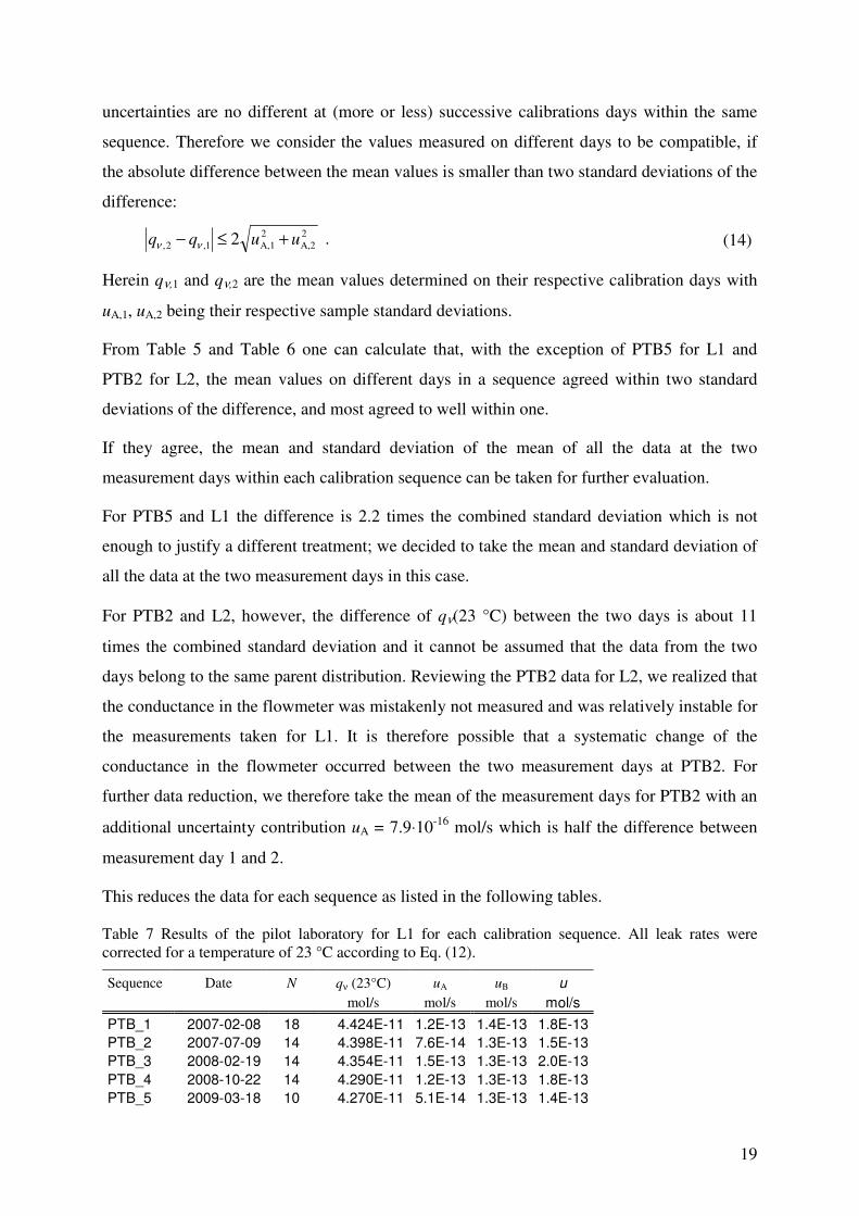
For PTB5 and L1 the difference is 2.2 times the combined standard deviation which is not

enough to justify a different treatment; we decided to take the mean and standard deviation of

all the data at the two measurement days in this case.

For PTB2 and L2, however, the difference of qν(23 °C) between the two days is about 11

times the combined standard deviation and it cannot be assumed that the data from the two

days belong to the same parent distribution. Reviewing the PTB2 data for L2, we realized that

the conductance in the flowmeter was mistakenly not measured and was relatively instable for

the measurements taken for L1. It is therefore possible that a systematic change of the

conductance in the flowmeter occurred between the two measurement days at PTB2. For

further data reduction, we therefore take the mean of the measurement days for PTB2 with an

additional uncertainty contribution uA = 7.9⋅10-16 mol/s which is half the difference between

measurement day 1 and 2.

This reduces the data for each sequence as listed in the following tables.

Table 7 Results of the pilot laboratory for L1 for each calibration sequence. All leak rates were corrected for a temperature of 23 °C according to Eq. (12).

Sequence Date N qν (23°C) uA uB u

mol/s mol/s mol/s mol/s

PTB_1 2007-02-08 18 4.424E-11 1.2E-13 1.4E-13 1.8E-13

PTB_2 2007-07-09 14 4.398E-11 7.6E-14 1.3E-13 1.5E-13

PTB_3 2008-02-19 14 4.354E-11 1.5E-13 1.3E-13 2.0E-13

PTB_4 2008-10-22 14 4.290E-11 1.2E-13 1.3E-13 1.8E-13

PTB_5 2009-03-18 10 4.270E-11 5.1E-14 1.3E-13 1.4E-13

2A,2

2A,11,2, 2 uuqq +≤− νν

20

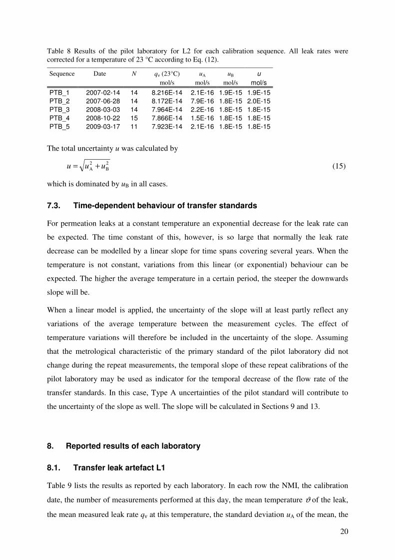
Table 8 Results of the pilot laboratory for L2 for each calibration sequence. All leak rates were corrected for a temperature of 23 °C according to Eq. (12).

Sequence Date N qν (23°C) uA uB u


PTB_1 2007-02-14 14 8.216E-14 2.1E-16 1.9E-15 1.9E-15

PTB_2 2007-06-28 14 8.172E-14 7.9E-16 1.8E-15 2.0E-15

PTB_3 2008-03-03 14 7.964E-14 2.2E-16 1.8E-15 1.8E-15

PTB_4 2008-10-22 15 7.866E-14 1.5E-16 1.8E-15 1.8E-15

PTB_5 2009-03-17 11 7.923E-14 2.1E-16 1.8E-15 1.8E-15

The total uncertainty u was calculated by

2B

2A uuu += (15)

which is dominated by uB in all cases.

7.3. Time-dependent behaviour of transfer standards

For permeation leaks at a constant temperature an exponential decrease for the leak rate can

be expected. The time constant of this, however, is so large that normally the leak rate

decrease can be modelled by a linear slope for time spans covering several years. When the

temperature is not constant, variations from this linear (or exponential) behaviour can be

expected. The higher the average temperature in a certain period, the steeper the downwards

slope will be.

When a linear model is applied, the uncertainty of the slope will at least partly reflect any

variations of the average temperature between the measurement cycles. The effect of

temperature variations will therefore be included in the uncertainty of the slope. Assuming

that the metrological characteristic of the primary standard of the pilot laboratory did not

change during the repeat measurements, the temporal slope of these repeat calibrations of the

pilot laboratory may be used as indicator for the temporal decrease of the flow rate of the

transfer standards. In this case, Type A uncertainties of the pilot standard will contribute to

the uncertainty of the slope as well. The slope will be calculated in Sections 9 and 13.

8. Reported results of each laboratory

8.1. Transfer leak artefact L1

Table 9 lists the results as reported by each laboratory. In each row the NMI, the calibration

date, the number of measurements performed at this day, the mean temperature ϑ of the leak,

the mean measured leak rate qν at this temperature, the standard deviation uA of the mean, the

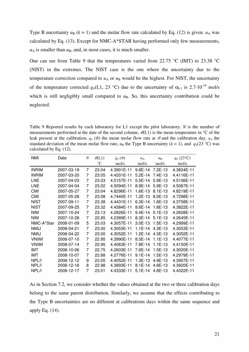
21

Type B uncertainty uB (k = 1) and the molar flow rate calculated by Eq. (12) is given. uA was

calculated by Eq. (13). Except for NMC-A*STAR having performed only few measurements,

uA is smaller than uB, and, in most cases, it is much smaller.

One can see from Table 9 that the temperatures varied from 22.75 °C (IMT) to 23.38 °C

(NIST) in the extremes. The NIST case is the one where the uncertainty due to the

temperature correction compared to uA or uB would be the highest. For NIST, the uncertainty

of the temperature corrected qν(L1, 23 °C) due to the uncertainty of αL1 is 2.7·10-14 mol/s

which is still negligibly small compared to uB. So, this uncertainty contribution could be

neglected.

Table 9 Reported results by each laboratory for L1 except the pilot laboratory. N is the number of measurements performed at the date of the second column, ϑ(L1) is the mean temperature in °C of the leak present at the calibration, qν (ϑ) the mean molar flow rate at ϑ and the calibration day, uA the standard deviation of the mean molar flow rate, uB the Type B uncertainty (k = 1), and qν(23 °C) was calculated by Eq. (12).

NMI Date N ϑ(L1) qν (ϑ) uA uB qν (23°C) °C mol/s mol/s mol/s mol/s

INRIM 2007-03-19 7 23.04 4.3901E-11 9.8E-14 7.2E-13 4.3824E-11

INRIM 2007-03-20 7 23.05 4.4201E-11 5.2E-14 7.4E-13 4.4116E-11

LNE 2007-04-03 7 23.03 4.5157E-11 5.5E-14 5.9E-13 4.5106E-11

LNE 2007-04-04 7 23.02 4.5094E-11 8.9E-14 5.9E-13 4.5067E-11

CMI 2007-05-27 7 23.04 4.8296E-11 1.6E-13 8.1E-13 4.8219E-11

CMI 2007-05-28 7 23.08 4.7440E-11 1.2E-13 8.0E-13 4.7298E-11

NIST 2007-09-11 7 23.38 4.4431E-11 6.3E-14 1.6E-13 4.3758E-11

NIST 2007-09-25 7 23.32 4.4384E-11 8.6E-14 1.8E-13 4.3822E-11

NIM 2007-10-24 7 23.13 4.2826E-11 9.4E-14 5.1E-13 4.2608E-11

NIM 2007-10-28 7 22.85 4.2389E-11 8.3E-14 5.1E-13 4.2645E-11

NMC-A*Star 2008-01-09 5 23.03 4.3057E-11 3.0E-13 1.5E-13 4.2999E-11

NMIJ 2008-04-21 7 23.00 4.3053E-11 1.1E-14 4.3E-13 4.3053E-11

NMIJ 2008-04-22 7 23.00 4.3052E-11 1.2E-14 4.3E-13 4.3052E-11

VNIIM 2008-07-10 7 22.95 4.3990E-11 8.5E-14 1.1E-13 4.4077E-11

VNIIM 2008-07-14 7 22.95 4.4063E-11 7.8E-14 1.1E-13 4.4150E-11

IMT 2008-10-06 7 22.75 4.2603E-11 7.6E-14 1.5E-13 4.3020E-11

IMT 2008-10-07 7 22.88 4.2776E-11 9.1E-14 1.5E-13 4.2979E-11

NPL/I 2008-12-12 9 23.05 4.4052E-11 1.3E-13 4.9E-13 4.3957E-11 NPL/I 2008-12-16 8 22.98 4.3893E-11 8.1E-14 4.8E-13 4.3920E-11

NPL/I 2008-12-17 7 23.01 4.4333E-11 5.1E-14 4.8E-13 4.4322E-11

As in Section 7.2, we consider whether the values obtained at the two or three calibration days

belong to the same parent distribution. Similarly, we assume that the effects contributing to

the Type B uncertainties are no different at calibrations days within the same sequence and

apply Eq. (14).

22

The differences between calibration days of INRIM, CMI and NPL/I (in 2 of 3 cases) violated

Eq. (14). As outlined in Section 7.2, for further data reduction we took the mean of the

measurements made on subsequent days with an additional uncertainty contribution which is

half the difference between measurement day 1 and 2 or, in the case of NPL/I, the standard

deviation of the mean values of measurements made on 3 calibration days.

In all other cases, we took the mean and standard deviation of all measurement data. The

results are shown in Table 10.

Table 10 Reduced data of L1 for each calibration sequence and for all participants except the pilot laboratory. uA is the standard deviation of the mean molar flow rate of all data of an NMI within its calibration sequence, uB the Type B uncertainty (k = 1), and u the total uncertainty (Eq. (15)). The results of the pilot laboratory are given in Table 7. All uncertainties are standard (k=1) values.

NMI Date qν (23°C) uA uB u


INRIM 2007-03-20 4.397E-11 1.5E-13 7.3E-13 7.5E-13

LNE 2007-04-04 4.509E-11 5.1E-14 5.9E-13 5.9E-13

CMI 2007-05-28 4.776E-11 4.3E-13 8.1E-13 9.2E-13

NIST 2007-09-25 4.379E-11 5.2E-14 1.7E-13 1.8E-13

NIM 2007-10-28 4.263E-11 8.6E-14 5.1E-13 5.2E-13 NMC-A*Star 2008-01-09 4.300E-11 3.0E-13 1.5E-13 3.4E-13

NMIJ 2008-04-22 4.305E-11 7.6E-15 4.3E-13 4.3E-13

VNIIM 2008-07-14 4.411E-11 5.6E-14 1.1E-13 1.2E-13

IMT 2008-10-07 4.300E-11 6.2E-14 1.5E-13 1.6E-13

NPL/I 2008-12-17 4.407E-11 2.2E-13 4.8E-13 5.3E-13

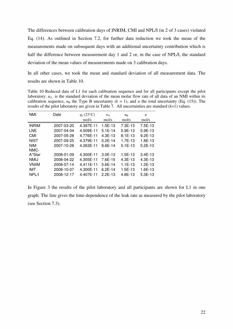
In Figure 3 the results of the pilot laboratory and all participants are shown for L1 in one

graph. The line gives the time-dependence of the leak rate as measured by the pilot laboratory

(see Section 7.3).

23

Figure 3 Illustration of the mean measured leak rates for L1 of each calibration sequence of the pilot laboratory (PTB) and the participants. The uncertainty bars are given as two times the combined standard uncertainty U=2u (k=2). The line is the temporal slope as determined by the pilot laboratory.

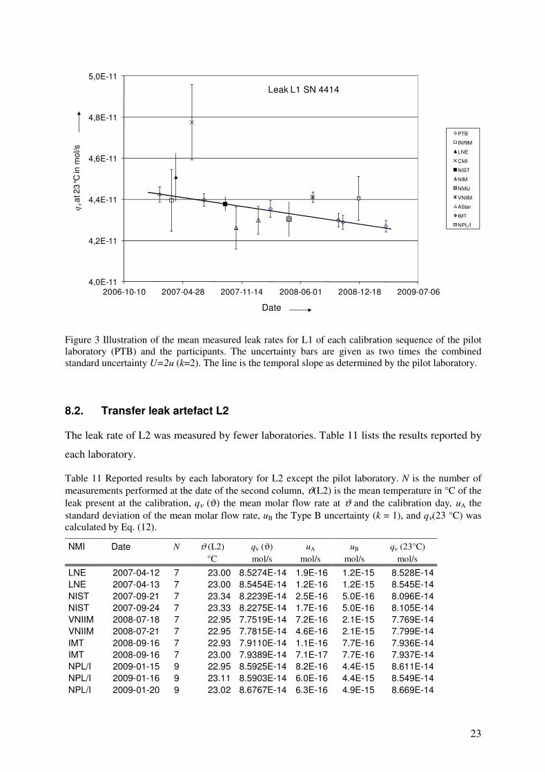
8.2. Transfer leak artefact L2

The leak rate of L2 was measured by fewer laboratories. Table 11 lists the results reported by

each laboratory.

Table 11 Reported results by each laboratory for L2 except the pilot laboratory. N is the number of measurements performed at the date of the second column, ϑ(L2) is the mean temperature in °C of the leak present at the calibration, qν (ϑ) the mean molar flow rate at ϑ and the calibration day, uA the standard deviation of the mean molar flow rate, uB the Type B uncertainty (k = 1), and qν(23 °C) was calculated by Eq. (12).

NMI Date N ϑ (L2) qν (ϑ) uA uB qν (23°C) °C mol/s mol/s mol/s mol/s

LNE 2007-04-12 7 23.00 8.5274E-14 1.9E-16 1.2E-15 8.528E-14

LNE 2007-04-13 7 23.00 8.5454E-14 1.2E-16 1.2E-15 8.545E-14

NIST 2007-09-21 7 23.34 8.2239E-14 2.5E-16 5.0E-16 8.096E-14

NIST 2007-09-24 7 23.33 8.2275E-14 1.7E-16 5.0E-16 8.105E-14

VNIIM 2008-07-18 7 22.95 7.7519E-14 7.2E-16 2.1E-15 7.769E-14

VNIIM 2008-07-21 7 22.95 7.7815E-14 4.6E-16 2.1E-15 7.799E-14

IMT 2008-09-16 7 22.93 7.9110E-14 1.1E-16 7.7E-16 7.936E-14

IMT 2008-09-16 7 23.00 7.9389E-14 7.1E-17 7.7E-16 7.937E-14

NPL/I 2009-01-15 9 22.95 8.5925E-14 8.2E-16 4.4E-15 8.611E-14

NPL/I 2009-01-16 9 23.11 8.5903E-14 6.0E-16 4.4E-15 8.549E-14

NPL/I 2009-01-20 9 23.02 8.6767E-14 6.3E-16 4.9E-15 8.669E-14

4,0E-11

4,2E-11

4,4E-11

4,6E-11

4,8E-11

5,0E-11

2006-10-10 2007-04-28 2007-11-14 2008-06-01 2008-12-18 2009-07-06

qνa

t 2

3°C

in m

ol/s

Date

PTB

INRIM

LNE

CMI

NIST

NIM

NMIJ

VNIIM

AStar

IMT

NPL/I

Leak L1 SN 4414

24

Here again, the NIST case is the one where the uncertainty due to the temperature correction

compared to uA or uB would be the highest. For NIST, the uncertainty of the temperature

corrected qν(L2, 23 °C) due to the uncertainty of αL2 is 1.4·10-17 mol/s which is negligibly

small compared to uA and uB. So, this uncertainty contribution could be neglected for L2 as

well.

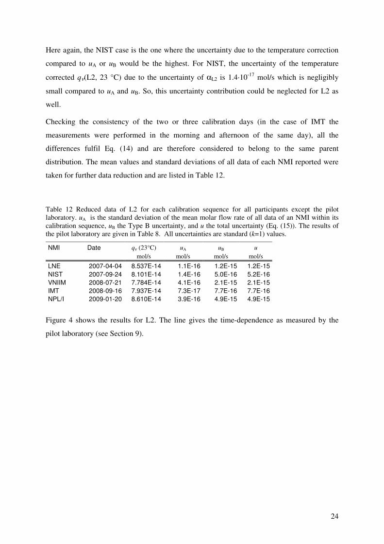
Checking the consistency of the two or three calibration days (in the case of IMT the

measurements were performed in the morning and afternoon of the same day), all the

differences fulfil Eq. (14) and are therefore considered to belong to the same parent

distribution. The mean values and standard deviations of all data of each NMI reported were

taken for further data reduction and are listed in Table 12.

Table 12 Reduced data of L2 for each calibration sequence for all participants except the pilot laboratory. uA is the standard deviation of the mean molar flow rate of all data of an NMI within its calibration sequence, uB the Type B uncertainty, and u the total uncertainty (Eq. (15)). The results of the pilot laboratory are given in Table 8. All uncertainties are standard (k=1) values.

NMI Date qν (23°C) uA uB u


LNE 2007-04-04 8.537E-14 1.1E-16 1.2E-15 1.2E-15

NIST 2007-09-24 8.101E-14 1.4E-16 5.0E-16 5.2E-16

VNIIM 2008-07-21 7.784E-14 4.1E-16 2.1E-15 2.1E-15

IMT 2008-09-16 7.937E-14 7.3E-17 7.7E-16 7.7E-16

NPL/I 2009-01-20 8.610E-14 3.9E-16 4.9E-15 4.9E-15

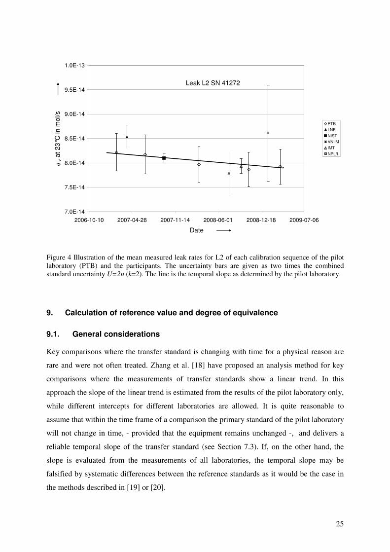
Figure 4 shows the results for L2. The line gives the time-dependence as measured by the

pilot laboratory (see Section 9).

25

Figure 4 Illustration of the mean measured leak rates for L2 of each calibration sequence of the pilot laboratory (PTB) and the participants. The uncertainty bars are given as two times the combined standard uncertainty U=2u (k=2). The line is the temporal slope as determined by the pilot laboratory.

9. Calculation of reference value and degree of equivalence

9.1. General considerations

Key comparisons where the transfer standard is changing with time for a physical reason are

rare and were not often treated. Zhang et al. [18] have proposed an analysis method for key

comparisons where the measurements of transfer standards show a linear trend. In this

approach the slope of the linear trend is estimated from the results of the pilot laboratory only,

while different intercepts for different laboratories are allowed. It is quite reasonable to

assume that within the time frame of a comparison the primary standard of the pilot laboratory

will not change in time, - provided that the equipment remains unchanged -, and delivers a

reliable temporal slope of the transfer standard (see Section 7.3). If, on the other hand, the

slope is evaluated from the measurements of all laboratories, the temporal slope may be

falsified by systematic differences between the reference standards as it would be the case in

the methods described in [19] or [20].

7.0E-14

7.5E-14

8.0E-14

8.5E-14

9.0E-14

9.5E-14

1.0E-13

2006-10-10 2007-04-28 2007-11-14 2008-06-01 2008-12-18 2009-07-06

Date

qν a

t 2

3°C

in m

ol/s

PTB

LNE

NIST

VNIIM

IMT

NPL/I

Leak L2 SN 41272

26

The method of Zhang [18], however, does not recognize a feature common to many inter-

laboratory studies, including KCs: that the inter-laboratory dispersion of measured values is

comparable to, or larger than the measurement uncertainty that the participating laboratories

associate with their own estimates of the measurand. This situation manifests itself in the

presence of measured values that appear to be too far away from the reference value ref,νq as

judged in terms of the associated measurement uncertainty. Unfortunately, this was the case

for data sets of CCM.P-K12. For this reason we did not use Zhang's approach for the final

evaluation and present the results in the appendix only (see Appendix Section 13.1).

The same issue has been observed in key comparisons with a stable measurand, and a

common remedy is to compute the key comparison reference value using a random effects

model that explicitly recognizes the possibility that the between-laboratory variability may

exceed the typical measurement uncertainty associated with the individual measured values

[24]-[26].

An alternative approach was recently developed by Bodnar et al. [21], which extended the

analysis of key comparisons by using Bayesian model averaging with a stable transfer

standard [22] to the case where the transfer standard has a linear trend. This method considers

the possibility that the reported values of some labs may contain an unknown bias by a fixed

amount (fixed effect Bayesian model averaging). This method, however, at present is not

completely consistent with the MRA, because this requires in the Technical Supplement T.2

that the degree of equivalence of each national measurement standard is expressed

quantitatively by its deviation from the key comparison reference value and the uncertainty of

this deviation. In the approach by Bodnar, however, the differences are determined by a

statistical averaging method. The evaluation of Bodnar et al. [21] will be summarized in the

Appendix Section 13.2.

For this reason, we finally applied an evaluation method which both considered possible

biases between laboratories and which is MRA consistent. It is based on a random effects

model that explicitly recognizes the possibility that the between-laboratory variability may

exceed the typical measurement uncertainty associated with the individual measured values

[24]-[26]. Producing a key comparison reference value using a random effects model is best

done numerically because closed form solutions generally are not available. Also, degrees of

equivalence can be computed as defined in the MRA: differences between values measured

by participating laboratories and the key comparison reference value, with associated

uncertainties computed consistently with the random effects model.

27

As the Zhang method, the random effect model extended to a linear trend method relies on the

slope as determined by the pilot laboratory.

9.2. Evaluation method and results

Although we apply the random effect model for evaluation, some elements from the Zhang

model (see Appendix Section 13.1) are useful to describe here. Following the approach of

Zhang et al. [18] , in order to have a coherent notation of the indices we will use the following

scheme:

i (1,2) is the index for the transfer leak element L1 or L2. If i is not specified, the equation is

true for either leak element.

j denotes the laboratory (j = 1…Ni, N1=11 for L1, N2=6 for L2), where j=1 is the pilot

laboratory (PTB).

k (1…5) is the temporal sequence of measurement series at the pilot laboratory during the

comparison.

l is the index for repeat measurements on a single day of a single measurement series.

In Zhang's approach, the reference value is calculated at a mean time t* during the course of

the comparison calculated from the times of all participants weighted by their respective

uncertainties. We will call t* as the reference time in the following. It is

∑=

∗ =Ni

j

jj twt1

, (16)

where tj are the times, when laboratory j performed the measurements1, and the weights wj are

given by

( )∑=

=Ni

j

j

j

j

u

uw

1

2,1

2

1

1 .

(17)

The uj are calculated from Eq.(14).

As described above, the downward trend of the measurements of the participating laboratories

is modelled by straight lines. Let β be the (negative) temporal slope as determined by the pilot

laboratory and αj the intersection at t=0, which is different for each laboratory. The predicted

value for each laboratory based on the trend is

( ) ∗+= ttq jj βα* . (18)

1 If the measurements were taken on consecutive days, the second day is taken, if the time period was larger, the average is taken.

28

In [18], a key comparison reference value qν,ref is given by

( )*1

ref, tqwqNi

j

jjν ∑=

= , (19)

and its uncertainty by

( )∑=

=Ni

j

j

q

u

uref

1

21

1,ν

. (20)

We compute ��,ref� , similar to ��,ref , using a random effects model. Specifically, we assume

that the qj(t*) from (18) are outcomes of Gaussian random variables with expected values

equal to µ + λi, where µ is the measurand at time t* , and λi are random laboratory differences

modelled as Gaussian random variables with mean 0 and variance �. The key comparison

reference value is

( )∑=

=Ni

j

jjref tqwq1

***,ν , (21)

where

∑=′ ′+

+=

Ni

j j

j

j

u

uw

122

22*

ˆ1

ˆ1

λ

λ

σ

σ

(22)

and 2ˆλσ is a maximum likelihood estimate of 2

λσ . Its uncertainty *

,refquν

is based on the

individual laboratory uncertainties and the inter-laboratory variance 2λσ . The estimates 2ˆ

λσ

and *

,refquν

(and therefore *,refqν ) are not available in closed form but are obtained numerically

(for more detail on maximum likelihood estimation see for example [24], Eqs. (13) and (14)]).

For this key comparison the estimation was done using an equivalent Bayesian procedure (see

[24], Section 6 therein) using the software OpenBUGS [27] and the code is included below

(Appendix Section 13.3). Once *,refqν is computed, the degrees of equivalence jD are

calculated in the usual way, as required by the MRA, as differences between the key

comparison reference value *,refqν and the laboratory value ( )*

tq j . The uncertainties Dju are

obtained numerically as posterior standard deviations of the differences.

To obtain ( )*tq j , the slope and intercepts were computed as in [18] using the pilot laboratory

data with uncertainties as

2B

2A uuu +=

. (23)

29

These formulas and the procedure are applied for both transfer standards L1 and L2 and their

reference values will be named *1,νq and *

2,νq respectively.

For element L1, the results were as follows.

.mol/s)/a(10)92.057.7( 131

−⋅±−=β (24)

"a" means the period of 1 year. The value of t* was determined to be

.d381* =t (25)

The key comparison reference value and its uncertainty was calculated based on the random

effects model using the OpenBUGS code to be

. mol/s10)0249.03746.4( 111,

−∗ ⋅±=νq (26)

As common practice, the degree of equivalence En is quantified by

Dj

j

nu

DE

2=

,

(27)

where Dj is the difference of the predicted value of laboratory j to the reference value and uDj

its uncertainty.

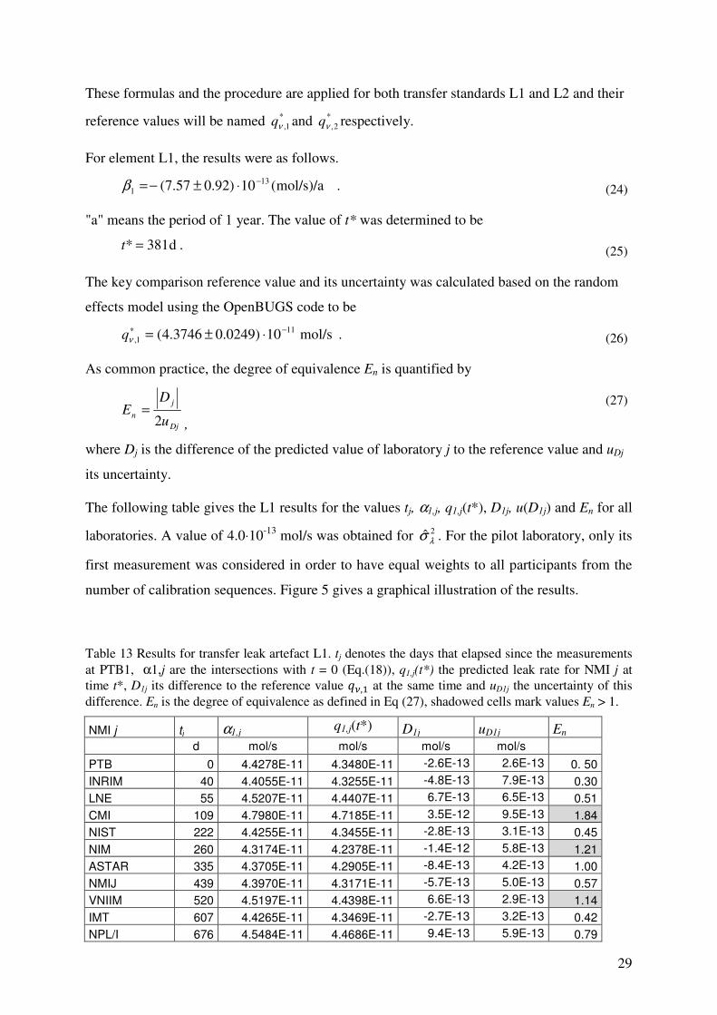
The following table gives the L1 results for the values tj, α1,j, q1,j(t*), D1j, u(D1j) and En for all

laboratories. A value of 4.0⋅10-13 mol/s was obtained for 2ˆλσ . For the pilot laboratory, only its

first measurement was considered in order to have equal weights to all participants from the

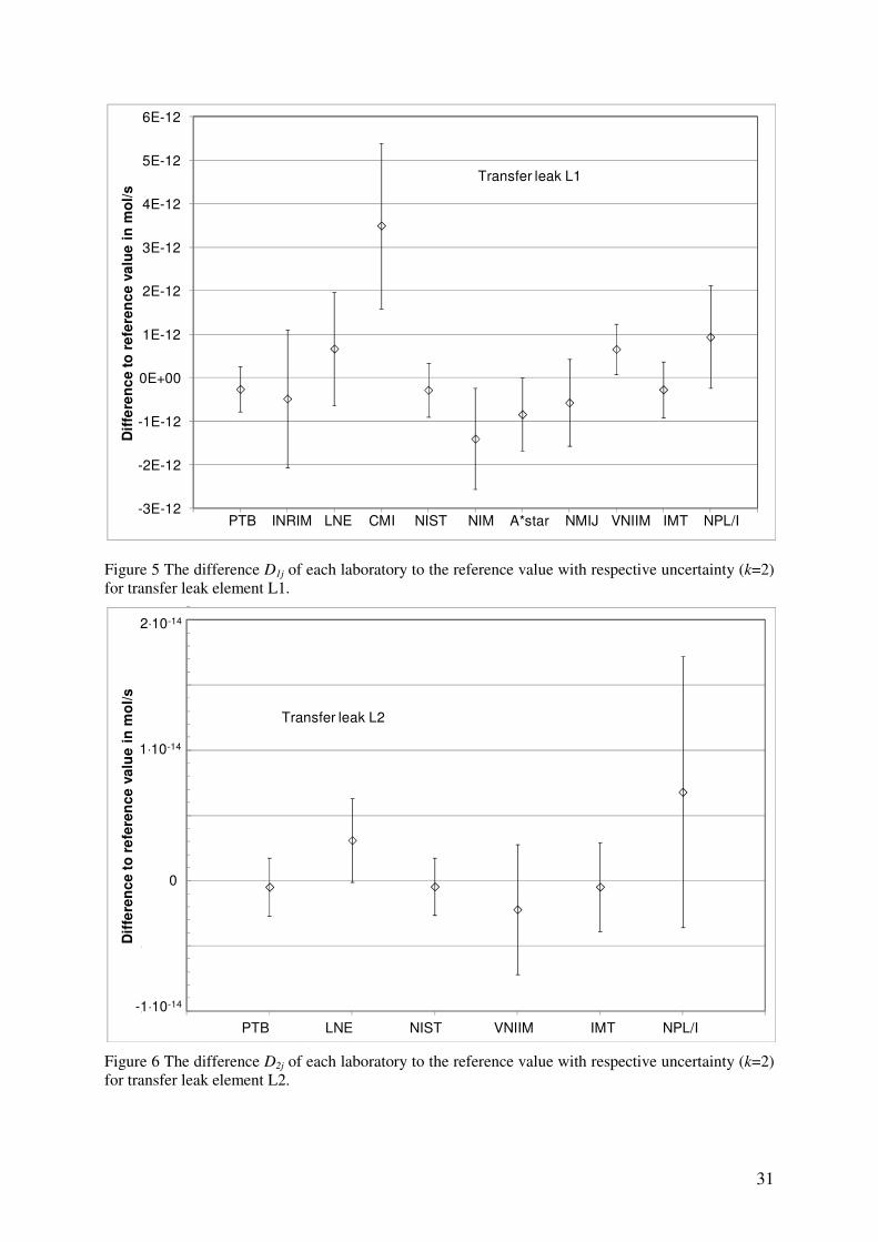
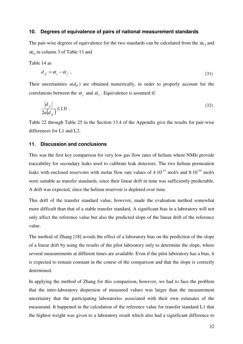
number of calibration sequences. Figure 5 gives a graphical illustration of the results.

Table 13 Results for transfer leak artefact L1. tj denotes the days that elapsed since the measurements at PTB1, α1,j are the intersections with t = 0 (Eq.(18)), q1,j(t*) the predicted leak rate for NMI j at time t*, D1j its difference to the reference value ��,� at the same time and uD1j the uncertainty of this difference. En is the degree of equivalence as defined in Eq (27), shadowed cells mark values En > 1.

NMI j tj α1,j q1,j(t*) D1j uD1j En

d mol/s mol/s mol/s mol/s

PTB 0 4.4278E-11 4.3480E-11 -2.6E-13 2.6E-13 0. 50

INRIM 40 4.4055E-11 4.3255E-11 -4.8E-13 7.9E-13 0.30

LNE 55 4.5207E-11 4.4407E-11 6.7E-13 6.5E-13 0.51

CMI 109 4.7980E-11 4.7185E-11 3.5E-12 9.5E-13 1.84

NIST 222 4.4255E-11 4.3455E-11 -2.8E-13 3.1E-13 0.45

NIM 260 4.3174E-11 4.2378E-11 -1.4E-12 5.8E-13 1.21

ASTAR 335 4.3705E-11 4.2905E-11 -8.4E-13 4.2E-13 1.00

NMIJ 439 4.3970E-11 4.3171E-11 -5.7E-13 5.0E-13 0.57

VNIIM 520 4.5197E-11 4.4398E-11 6.6E-13 2.9E-13 1.14

IMT 607 4.4265E-11 4.3469E-11 -2.7E-13 3.2E-13 0.42

NPL/I 676 4.5484E-11 4.4686E-11 9.4E-13 5.9E-13 0.79

30

Table 13 shows that 3 of 11 En values are > 1 indicating good consistency for most of the

other laboratories. Note that the values of q1,j(t*) of PTB, NIST and IMT differ only in the

fourth digit by a maximum of relative difference of 5.8⋅10-4.

NPL/I is consistent with the reference value, but the En-value would be smaller when the error

in the volume (see Section 3.9) would be considered.

For transfer standard L2 the slope parameter was

.mol/s)/a(10)06.165.1( 152

−⋅±−=β (28)

t* was determined to be

d298* =t (29)

The key comparison reference value and its uncertainty was calculated to be

. mol/s10)072.0111.8( 142

−∗ ⋅±=q (30)

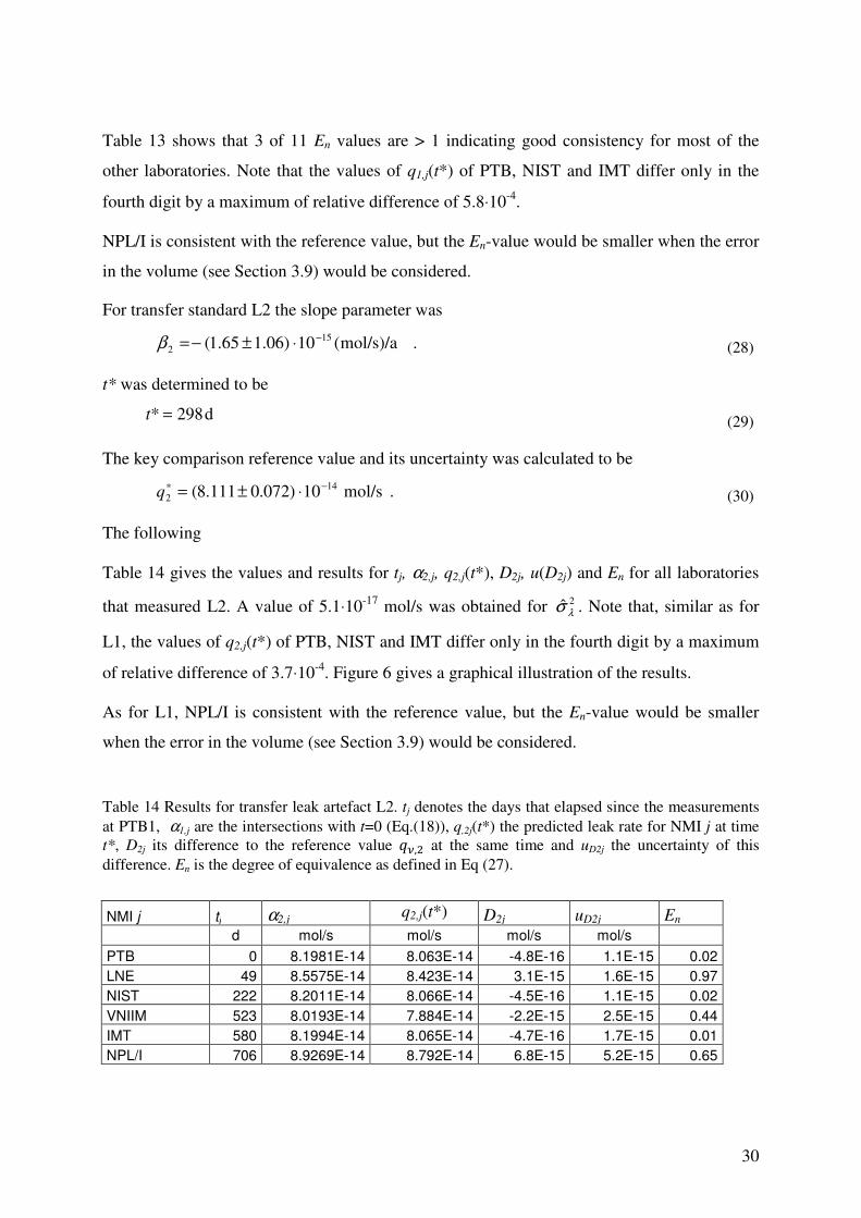
The following

Table 14 gives the values and results for tj, α2,j, q2,j(t*), D2j, u(D2j) and En for all laboratories

that measured L2. A value of 5.1⋅10-17 mol/s was obtained for 2ˆλσ . Note that, similar as for

L1, the values of q2,j(t*) of PTB, NIST and IMT differ only in the fourth digit by a maximum

of relative difference of 3.7⋅10-4. Figure 6 gives a graphical illustration of the results.

As for L1, NPL/I is consistent with the reference value, but the En-value would be smaller

when the error in the volume (see Section 3.9) would be considered.

Table 14 Results for transfer leak artefact L2. tj denotes the days that elapsed since the measurements at PTB1, α1,j are the intersections with t=0 (Eq.(18)), q,2j(t*) the predicted leak rate for NMI j at time t*, D2j its difference to the reference value ��, at the same time and uD2j the uncertainty of this difference. En is the degree of equivalence as defined in Eq (27).

NMI j tj α2,j q2,j(t*) D2j uD2j En d mol/s mol/s mol/s mol/s

PTB 0 8.1981E-14 8.063E-14 -4.8E-16 1.1E-15 0.02

LNE 49 8.5575E-14 8.423E-14 3.1E-15 1.6E-15 0.97

NIST 222 8.2011E-14 8.066E-14 -4.5E-16 1.1E-15 0.02

VNIIM 523 8.0193E-14 7.884E-14 -2.2E-15 2.5E-15 0.44

IMT 580 8.1994E-14 8.065E-14 -4.7E-16 1.7E-15 0.01

NPL/I 706 8.9269E-14 8.792E-14 6.8E-15 5.2E-15 0.65

31

Figure 5 The difference D1j of each laboratory to the reference value with respective uncertainty (k=2) for transfer leak element L1.

Figure 6 The difference D2j of each laboratory to the reference value with respective uncertainty (k=2) for transfer leak element L2.

-3E-12

-2E-12

-1E-12

0E+00

1E-12

2E-12

3E-12

4E-12

5E-12

6E-12D

iffe

ren

ce

to

re

fere

nc

e v

alu

e i

n m

ol/

s

PTB INRIM LNE CMI NIST NIM A*star NMIJ VNIIM IMT NPL/I

Transfer leak L1

-

-

Dif

fere

nc

e t

o r

efe

ren

ce

va

lue

in

mo

l/s

PTB LNE NIST VNIIM IMT NPL/I

0

1⋅10-14

2⋅10-14

-1⋅10-14

Transfer leak L2

32

10. Degrees of equivalence of pairs of national measurement standards

The pair-wise degrees of equivalence for the two standards can be calculated from the α1,j and

α2,j in column 3 of Table 13 and

Table 14 as

'' jjjjd αα −= , (31)

Their uncertainties u(djj’) are obtained numerically, in order to properly account for the

correlations between the jα and 'jα . Equivalence is assumed if:

( )0.1

2 '

'≤

jj

jj

du

d .

(32)

Table 22 through Table 25 in the Section 13.4 of the Appendix give the results for pair-wise

differences for L1 and L2.

11. Discussion and conclusions

This was the first key comparison for very low gas flow rates of helium where NMIs provide

traceability for secondary leaks used to calibrate leak detectors. The two helium permeation

leaks with enclosed reservoirs with molar flow rate values of 4⋅10-11 mol/s and 8⋅10-14 mol/s

were suitable as transfer standards, since their linear drift in time was sufficiently predictable.

A drift was expected, since the helium reservoir is depleted over time.

This drift of the transfer standard value, however, made the evaluation method somewhat

more difficult than that of a stable transfer standard. A significant bias in a laboratory will not

only affect the reference value but also the predicted slope of the linear drift of the reference

value.

The method of Zhang [18] avoids the effect of a laboratory bias on the prediction of the slope

of a linear drift by using the results of the pilot laboratory only to determine the slope, where

several measurements at different times are available. Even if the pilot laboratory has a bias, it

is expected to remain constant in the course of the comparison and that the slope is correctly

determined.

In applying the method of Zhang for this comparison, however, we had to face the problem

that the inter-laboratory dispersion of measured values was larger than the measurement

uncertainty that the participating laboratories associated with their own estimates of the

measurand. It happened in the calculation of the reference value for transfer standard L1 that

the highest weight was given to a laboratory result which also had a significant difference to

33

most of the other laboratories (see Appendix Section 13.1). As a consequence, 10 of the 11

participants had a difference from the reference value of more than one standard uncertainty

which was a highly improbable outcome.

For this reason, we extended the random effects model [24]-[26] to the case of a linear drift of

the transfer standard. By the random effects model one can handle the case that the dispersion

of measured values is larger than the measurement uncertainty at the expense of an increased

uncertainty of the calculated differences, i.e. the laboratory result minus reference value.

Applying this evaluation method, for transfer leak artefact L1, 3 laboratory results exhibited

En values > 1. One of these laboratories, the CMI, also showed En values > 1 with all other

laboratories in the pair-wise differences (Table 23 in Section 13.4), while the other 2, NIM

and VNIIM, showed En values > 1 with 7 of the other 10 laboratories.

For transfer leak L2, where only 6 laboratories supplied data, all values were consistent with

the reference value. The pair-wise differences of LNE, however, showed En values > 1 with 2

of the 5 other laboratories.

For the evaluation of this comparison we also tested the method using Bayesian model

averaging with a fixed effect (Section 13.2). Here, a possible bias between laboratories is

considered by an additional fixed term, while the method using a random effects model

assumes that this bias term may vary when the experiment would be repeated. In other words,

in the first case it is assumed that the measurand might be not properly estimated by the

laboratory, while in the second case it is assumed that the uncertainty of the measurand might

not be properly estimated.

This method had the tendency that the results for the En-values were lower for most of the

laboratories compared to the En-values obtained by the random effect model and the Zhang

method. The exception were the En-values > 1. For L1, only the En-values of CMI and VNIIM

were larger than 1, while the En-value of NIM was < 1. The En-value of NIM was > 1 for the

other two methods. For L2, all laboratories were equivalent as in the random effect model.

None of the approaches to evaluate this KC was without weakness and none of these

approaches did satisfy us completely in terms of the metrological concept, consistency,

robustness and MRA conformity. We finally decided for the random effects model method,

which shows MRA conformity, but appeal to the statisticians to continue the work on the

evaluation of this comparison by a more detailed discussion of the methods presented and by

testing more methods.

34

12. References

[1] Ehrlich, C Basford, J A 1992 J. Vac. Sci. Technol. A 10 1-17 [2] Peggs GN 1976 Vacuum 26 321 [3] Peksa L Řepa P Gronych T Tesař J Pražák D 2004 Vacuum 76 477-489 [4] Tesar J Prazak D Stanek F Repa P Peksa L 2007 Vacuum 81 785-787 [5] Gronych, T Peksa L Řepa P Wild, J Tesař J Pražák D Krajíček Z 2008 Metrologia 45 46 - 52 [6] Peksa L Gronych T Řepa P Tesař J Vičar M Pražák DKrajíček Z.Wild J. 2008 Metrologia 45 2008, 368 –

375 [7] Peksa L et al 2008 J. Phys.: Conf. Ser. 100 092009 (4pp) doi: 10.1088/1742-6596/100/9/092009 [8] Erjavec B Šetina J Design 2003 XVII IMEKO World Congress, Dubrovnik, Croatia Zagreb: HMD -

Croatian Metrology Society, 135-137. [9] Calcatelli A Raiteri G Rumiano G 2003 Measurement 34 121-132 [10] McCulloh KE Tilford CR Ehrlich CD Long FG 1987 J. Vac. Sci. Technol. A 5 376-381 [11] Wu J Chua H A 2006 XVIII IMEKO World Congress, Rio de Janeiro,

http://www.imeko.org/publications/wc-2006/PWC-2006-TC9-022u.pdf [12] Arai K, Akimichi H, Hirata M, 2010 J. Vac. Soc. Jpn 53 614-620 (in Japanese). [13] Mohan P 1998 Vacuum 51 69-74 [14] Tison S A Bergoglio M Rumanio G Mohan P Gupta A C 1999 MAPAN, J. Metro. Soc. of India 14 103-114 [15] Mohan P, Gupta A C 1999 Proc. of 8th ISMAS Symp. Mass Spectrometry ed. Aggarwal S K Vol. II 737-

740 [16] Mohan P 2003 MAPAN, J. Metro. Soc. of India 18 131-137 [17] Jousten K, Messer G, Wandrey D 1993 Vacuum 44 135 – 141 [18] Nien Fan Zhang, Hung-Kung Liu, Nell Sedransk, W.E. Strawdermann 2004 Metrologia 41 231-237 [19] Stepanov A V 2007 Measurement Techniques 50 1019-1027 [20] Elster C Wöger W Cox M 2005 Measurement Techniques 48 883-893 [21] Bodnar O Link A Klauenberg K Jousten K Elster C. Accepted by and to be published in Measurement

Techniques in Russian (2012) and English (2013). [22] Elster C Toman B 2010 Metrologia 47 113-119 [23] Cox M G 2007 Metrologia 44 187-200 [24] Rukhin (2009) Metrologia 46, 323 – 331 [25] Toman and Possolo (2009) Accreditation and Quality Assurance 14, 553 – 563 [26] Toman and Possolo (2010) (Errata) Accreditation and Quality Assurance 15, 653 – 654 [27] Lunn, D., Spiegelhalter, D., Thomas, A. and Best, N. (2009) The BUGS project: Evolution, critique and

future directions (with discussion), Statistics in Medicine 28: 3049--3082.

Acknowledgments

One of the authors (PM) acknowledges the contribution of Mr. Harish Kumar for help in data

collection.

35

13. Appendix

13.1. Alternative evaluation method by Zhang et al.

This section describes the evaluation method published by Zhang [18]. We follow the

notation described already in the beginning of Section 9.2. Continuing from Eq. (20) in the

same section the degree of equivalence is the difference Dj between the value of laboratory j

extrapolated for the reference time t* and the qν,ref:

refjj qtD ,νβα −+= ∗ , (33)

Herein β is the (negative) temporal slope as determined by the pilot laboratory and αj the

intersection at t=0, which is different for each laboratory. The quantity qj(t*)

( ) ∗+= ttq jj βα* , (34)

is the predicted leak rate for laboratory j, when all laboratories would have measured at the

same time t* .

αj is calculated from

jjj tq βα ν −= , . (35)

β is calculated from the five PTB measurement sequences being part of the comparison:

( )( )

( )∑

∑

=

=

−

−−

=5

1

21

5

11,,1,11

k

ik

k

kk

tt

qqtt νν

β

(36)

with its variance being

( )( )∑

∑

=

=

−

=5

1

21

5

1

2A,,1 5

Var

k

ik

k

k

tt

u

β .

(37)

ti is the average of the measurement sequences ti,k at the pilot laboratory and qν,i the mean

value

2,15

5

1,,

, ==∑

= i

q

q k

ki

i

ν

ν .

(38)

The corresponding uncertainty of Dj is

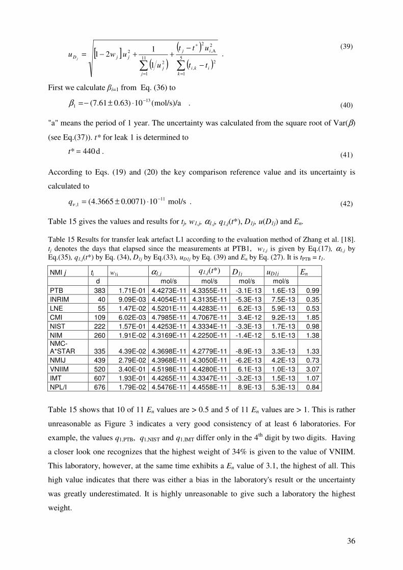
36

[ ]( )

( )

( )∑∑=

∗

=

−

−++−=

5

1

2,

2A,

2

11

1

2

2

1

121

k

iki

ij

j

j

jjD

tt

utt

u

uwuj

. (39)

First we calculate βi=1 from Eq. (36) to

.mol/s)/a(10)63.061.7( 131

−⋅±−=β (40)

"a" means the period of 1 year. The uncertainty was calculated from the square root of Var(β)

(see Eq.(37)). t* for leak 1 is determined to

.d440* =t (41)

According to Eqs. (19) and (20) the key comparison reference value and its uncertainty is

calculated to

. mol/s10)0071.03665.4( 111,

−⋅±=νq (42)

Table 15 gives the values and results for tj, w1,j, α1,j, q1,j(t*), D1j, u(D1j) and En.

Table 15 Results for transfer leak artefact L1 according to the evaluation method of Zhang et al. [18]. tj denotes the days that elapsed since the measurements at PTB1, w1,j is given by Eq.(17), α1,j by Eq.(35), q1,j(t*) by Eq. (34), D1j by Eq.(33), uD1j by Eq. (39) and En by Eq. (27). It is tPTB = t1.

NMI j tj w1j α1,j q1,j(t*) D1j uD1j En

d


PTB 383 1.71E-01 4.4273E-11 4.3355E-11 -3.1E-13 1.6E-13 0.99

INRIM 40 9.09E-03 4.4054E-11 4.3135E-11 -5.3E-13 7.5E-13 0.35

LNE 55 1.47E-02 4.5201E-11 4.4283E-11 6.2E-13 5.9E-13 0.53

CMI 109 6.02E-03 4.7985E-11 4.7067E-11 3.4E-12 9.2E-13 1.85

NIST 222 1.57E-01 4.4253E-11 4.3334E-11 -3.3E-13 1.7E-13 0.98

NIM 260 1.91E-02 4.3169E-11 4.2250E-11 -1.4E-12 5.1E-13 1.38

NMC-A*STAR 335 4.39E-02 4.3698E-11 4.2779E-11 -8.9E-13 3.3E-13 1.33

NMIJ 439 2.79E-02 4.3968E-11 4.3050E-11 -6.2E-13 4.2E-13 0.73

VNIIM 520 3.40E-01 4.5198E-11 4.4280E-11 6.1E-13 1.0E-13 3.07

IMT 607 1.93E-01 4.4265E-11 4.3347E-11 -3.2E-13 1.5E-13 1.07

NPL/I 676 1.79E-02 4.5476E-11 4.4558E-11 8.9E-13 5.3E-13 0.84

Table 15 shows that 10 of 11 En values are > 0.5 and 5 of 11 En values are > 1. This is rather

unreasonable as Figure 3 indicates a very good consistency of at least 6 laboratories. For

example, the values q1,PTB, q1,NIST and q1,IMT differ only in the 4th digit by two digits. Having

a closer look one recognizes that the highest weight of 34% is given to the value of VNIIM.

This laboratory, however, at the same time exhibits a En value of 3.1, the highest of all. This

high value indicates that there was either a bias in the laboratory's result or the uncertainty

was greatly underestimated. It is highly unreasonable to give such a laboratory the highest

weight.

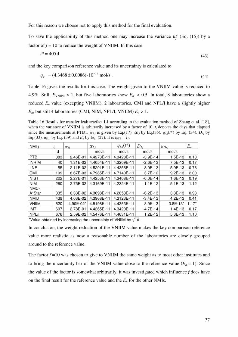
37

For this reason we choose not to apply this method for the final evaluation.

To save the applicability of this method one may increase the variance � (Eq. (15)) by a

factor of f = 10 to reduce the weight of VNIIM. In this case

d405* =t (43)

and the key comparison reference value and its uncertainty is calculated to

. mol/s10)0086.03468.4( 111,

−⋅±=νq (44)

Table 16 gives the results for this case. The weight given to the VNIIM value is reduced to

4.9%. Still, EVNIIM > 1, but five laboratories show En < 0.5. In total, 8 laboratories show a

reduced En value (excepting VNIIM), 2 laboratories, CMI and NPL/I have a slightly higher

En, but still 4 laboratories (CMI, NIM, NPL/I, VNIIM) En > 1.

Table 16 Results for transfer leak artefact L1 according to the evaluation method of Zhang et al. [18], when the variance of VNIIM is arbitrarily increased by a factor of 10. tj denotes the days that elapsed since the measurements at PTB1. w1,j is given by Eq.(17), α1,j by Eq.(35), q1,j(t*) by Eq. (34), D1j by Eq.(33), uD1j by Eq. (39) and En by Eq. (27). It is tPTB = t1.

NMI j tj w1j α1,j q1,j(t*) D1j uD1j En d


PTB 383 2.46E-01 4.4273E-11 4.3428E-11 -3.9E-14 1.5E-13 0.13

INRIM 40 1.31E-02 4.4054E-11 4.3209E-11 -2.6E-13 7.5E-13 0.17

LNE 55 2.11E-02 4.5201E-11 4.4356E-11 8.9E-13 5.9E-13 0.76

CMI 109 8.67E-03 4.7985E-11 4.7140E-11 3.7E-12 9.2E-13 2.00

NIST 222 2.27E-01 4.4253E-11 4.3408E-11 -6.0E-14 1.6E-13 0.19

NIM 260 2.75E-02 4.3169E-11 4.2324E-11 -1.1E-12 5.1E-13 1.12

NMC-A*Star 335 6.33E-02 4.3698E-11 4.2853E-11 -6.2E-13 3.3E-13 0.93

NMIJ 439 4.03E-02 4.3968E-11 4.3123E-11 -3.4E-13 4.2E-13 0.41

VNIIM 520 4.90E-02* 4.5198E-11 4.4353E-11 8.9E-13 3.8E-13* 1.17*

IMT 607 2.78E-01 4.4265E-11 4.3420E-11 -4.7E-14 1.4E-13 0.17

NPL/I 676 2.59E-02 4.5476E-11 4.4631E-11 1.2E-12 5.3E-13 1.10

*Value obtained by increasing the uncertainty of VNIIM by √10.

In conclusion, the weight reduction of the VNIIM value makes the key comparison reference

value more realistic as now a reasonable number of the laboratories are closely grouped

around to the reference value.

The factor f =10 was chosen to give to VNIIM the same weight as to most other institutes and

to bring the uncertainty bar of the VNIIM value close to the reference value (En ≅ 1). Since

the value of the factor is somewhat arbitrarily, it was investigated which influence f does have

on the final result for the reference value and the En for the other NMIs.

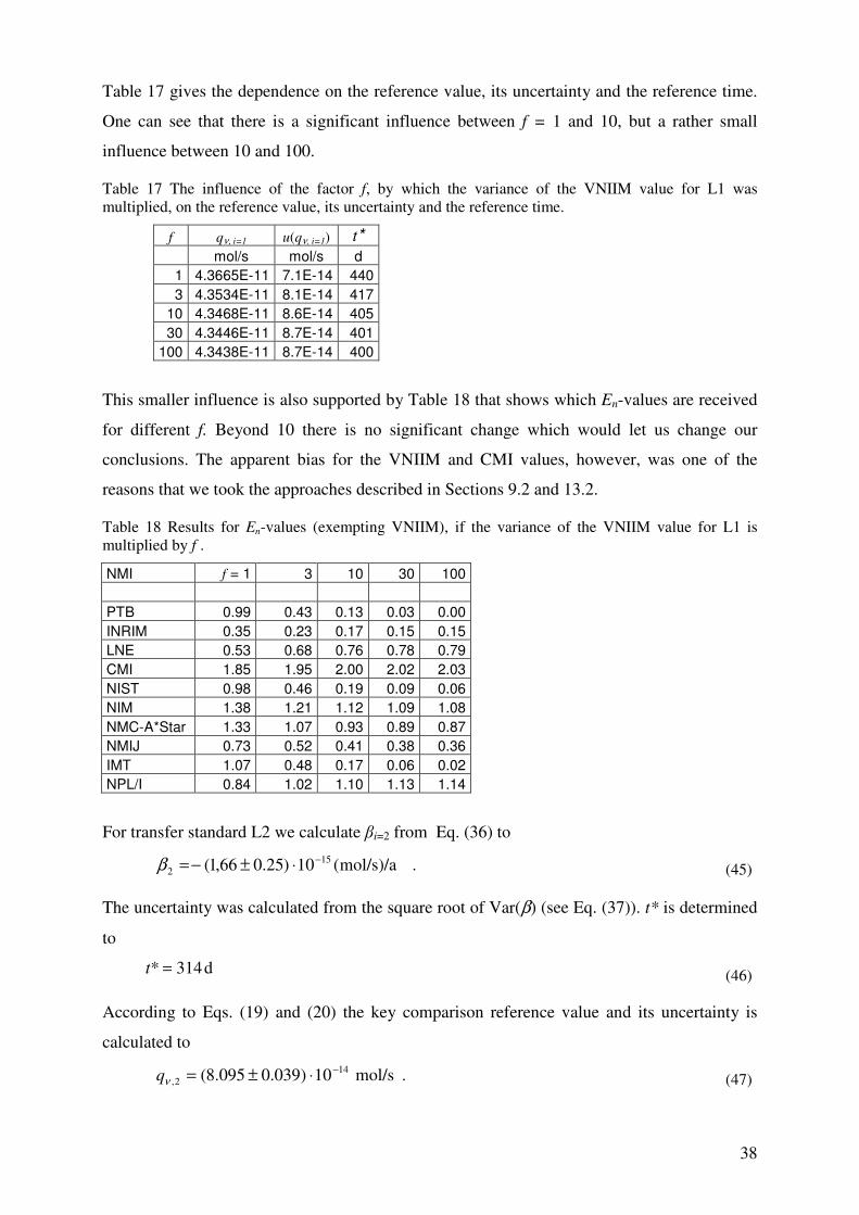
38

Table 17 gives the dependence on the reference value, its uncertainty and the reference time.

One can see that there is a significant influence between f = 1 and 10, but a rather small

influence between 10 and 100.

Table 17 The influence of the factor f, by which the variance of the VNIIM value for L1 was multiplied, on the reference value, its uncertainty and the reference time.

f qν, i=1 u(qν, i=1) t*

mol/s mol/s d

1 4.3665E-11 7.1E-14 440

3 4.3534E-11 8.1E-14 417

10 4.3468E-11 8.6E-14 405

30 4.3446E-11 8.7E-14 401

100 4.3438E-11 8.7E-14 400

This smaller influence is also supported by Table 18 that shows which En-values are received

for different f. Beyond 10 there is no significant change which would let us change our

conclusions. The apparent bias for the VNIIM and CMI values, however, was one of the

reasons that we took the approaches described in Sections 9.2 and 13.2.

Table 18 Results for En-values (exempting VNIIM), if the variance of the VNIIM value for L1 is multiplied by f .

NMI f = 1 3 10 30 100

PTB 0.99 0.43 0.13 0.03 0.00

INRIM 0.35 0.23 0.17 0.15 0.15

LNE 0.53 0.68 0.76 0.78 0.79

CMI 1.85 1.95 2.00 2.02 2.03

NIST 0.98 0.46 0.19 0.09 0.06

NIM 1.38 1.21 1.12 1.09 1.08

NMC-A*Star 1.33 1.07 0.93 0.89 0.87

NMIJ 0.73 0.52 0.41 0.38 0.36

IMT 1.07 0.48 0.17 0.06 0.02

NPL/I 0.84 1.02 1.10 1.13 1.14

For transfer standard L2 we calculate βi=2 from Eq. (36) to

.mol/s)/a(10)25.066,1( 152

−⋅±−=β (45)

The uncertainty was calculated from the square root of Var(β) (see Eq. (37)). t* is determined

to

d314* =t (46)

According to Eqs. (19) and (20) the key comparison reference value and its uncertainty is

calculated to

. mol/s10)039.0095.8( 142,

−⋅±=νq (47)

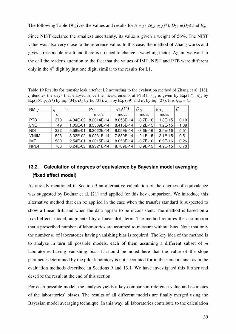
39

The following Table 19 gives the values and results for tj, w2,j, α2,j, q2,j(t*), D2j, u(D2j) and En.

Since NIST declared the smallest uncertainty, its value is given a weight of 56%. The NIST

value was also very close to the reference value. In this case, the method of Zhang works and

gives a reasonable result and there is no need to change a weighing factor. Again, we want to

the call the reader's attention to the fact that the values of IMT, NIST and PTB were different

only in the 4th digit by just one digit, similar to the results for L1.

Table 19 Results for transfer leak artefact L2 according to the evaluation method of Zhang et al. [18]. tj denotes the days that elapsed since the measurements at PTB1. w1,j is given by Eq.(17), α1,j by Eq.(35), q1,j(t*) by Eq. (34), D1j by Eq.(33), uD1j by Eq. (39) and En by Eq. (27). It is tPTB = t1.

NMI j tj w2j α2,j q2,j(t*) D2j uD2j En d


PTB 379 4.34E-02 8.2014E-14 8.058E-14 -3.7E-16 1.8E-15 0.10

LNE 49 1.05E-01 8.5589E-14 8.415E-14 3.2E-15 1.2E-15 1.39

NIST 222 5.58E-01 8.2022E-14 8.059E-14 -3.6E-16 3.5E-16 0.51

VNIIM 523 3.32E-02 8.0231E-14 7.880E-14 -2.1E-15 2.1E-15 0.51

IMT 580 2.54E-01 8.2015E-14 8.058E-14 -3.7E-16 6.9E-16 0.26

NPL/I 706 6.24E-03 8.9321E-14 8.789E-14 6.9E-15 4.9E-15 0.70

13.2. Calculation of degrees of equivalence by Bayesian model averaging

(fixed effect model)

As already mentioned in Section 9 an alternative calculation of the degrees of equivalence

was suggested by Bodnar et al. [21] and applied for this key comparison. We introduce this

alternative method that can be applied in the case when the transfer standard is suspected to

show a linear drift and when the data appear to be inconsistent. The method is based on a

fixed effects model, augmented by a linear drift term. The method requires the assumption

that a prescribed number of laboratories are assumed to measure without bias. Note that only

the number m of laboratories having vanishing bias is required. The key idea of the method is

to analyze in turn all possible models, each of them assuming a different subset of m

laboratories having vanishing bias. It should be noted here that the value of the slope

parameter determined by the pilot laboratory is not accounted for in the same manner as in the

evaluation methods described in Sections 9 and 13.1. We have investigated this further and

describe the result at the end of this section.

For each possible model, the analysis yields a key comparison reference value and estimates

of the laboratories’ biases. The results of all different models are finally merged using the

Bayesian model averaging technique. In this way, all laboratories contribute to the calculation

40

of the key comparison reference value (without identifying any ‘outliers’) and the final

estimates of the laboratories’ biases. These estimates then serve as the degrees of equivalence.

Let ),,( 11,1, ′= vv qqq K and ))(,),(( 11,1, ′= vv ququu K denote the estimates and corresponding

standard uncertainties for L1 reported by the 11 laboratories participating in this comparison,

and let 111 ,, tt K denote the (known) times when these measurements were carried out. We

model 11,1, ,, vv qq K as realizations of the random variables

,,,1,, niEtQ iiiiv K=+++= γβµ (48)

where ))(,0(~ ,2

ivi quNE is normally distributed with zero mean and variance )( ,2

ivqu . In

(48), itβµ + denotes the value of the measurand at time it , and iγ the bias of laboratory i.

The iγµ + can be identified with the αi in Eq. (35), since Zhang does not consider any bias.

Model (48) contains the 13 unknown parameters βµ, and 111 ,, γγ K . As there are only 11

observations 11,1, ,, vv qq K available, model (48) is not identifiable. We additionally assume

that reliable uncertainties have been quoted for an unknown set of m laboratories, i.e. that the

corresponding biases equal zero (see, e.g. [21])

},,{,0 1 mil llli

K∈=γ , (49)

where m is called the model order parameter. For the model to be identifiable 2≥m is

required. Subsequently, the model order parameter m is assumed to be fixed. That is, we

assume that m laboratories have no bias, but we do not specify (and do not identify) which.

The model order parameter m cannot be determined uniquely from the data and needs to be

assigned. Fortunately, the data provide some information as to an upper bound of this

parameter, since m cannot exceed the maximum number m of laboratories that form a

coherent subset. The upper bound m for m is derived as the number of laboratories in the

largest coherent subset of laboratories (cf. [21]).

In a first step, we consider all triples of laboratories and judge whether they report results that

are consistent with a linear drift model based on the �-value (see [21]).

Next we consider coherent subsets of the laboratories. We call a subset coherent if all its

triples are consistent with a linear drift model. The upper bound m for m is then determined

as the number of laboratories in the largest coherent subset. We recommend selecting

2−= mm (see [21]). Let T

ll p),...,,,(

1γγβµθ = with mp −= 11 denoting the vector of model

parameters under the specified model lM . First, we derive the posterior distribution of θ for

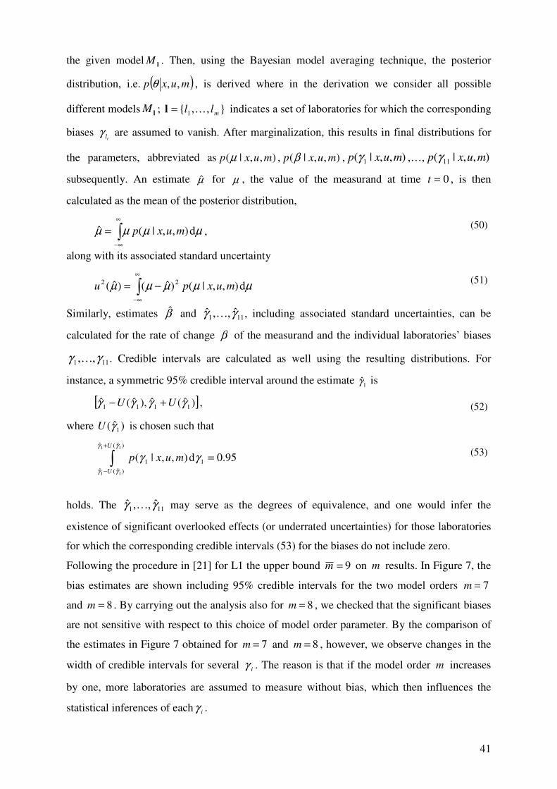
41

the given model lM . Then, using the Bayesian model averaging technique, the posterior

distribution, i.e. ( )muxp ,,θ , is derived where in the derivation we consider all possible

different models lM ; },,{ 1 mll K=l indicates a set of laboratories for which the corresponding

biases il

γ are assumed to vanish. After marginalization, this results in final distributions for

the parameters, abbreviated as ),,|( muxp µ , ),,|( muxp β , ),,|( 1 muxp γ ,…, ),,|( 11 muxp γ

subsequently. An estimate µ̂ for µ , the value of the measurand at time 0=t , is then

calculated as the mean of the posterior distribution,

∫∞

∞−

= µµµµ d),,|(ˆ muxp , (50)

along with its associated standard uncertainty

∫∞

∞−

−= µµµµµ d),,|()ˆ()ˆ( 22muxpu

(51)

Similarly, estimates β̂ and 111 ˆ,,ˆ γγ K , including associated standard uncertainties, can be

calculated for the rate of change β of the measurand and the individual laboratories’ biases

111 ,, γγ K . Credible intervals are calculated as well using the resulting distributions. For

instance, a symmetric 95% credible interval around the estimate 1γ̂ is

[ ])ˆ(ˆ),ˆ(ˆ 1111 γγγγ UU +− , (52)

where )ˆ( 1γU is chosen such that

95.0d),,|()ˆ(ˆ

)ˆ(ˆ11

11

11

=∫+

−

γγ

γγ

γγU

U

muxp (53)

holds. The 111 ˆ,,ˆ γγ K may serve as the degrees of equivalence, and one would infer the

existence of significant overlooked effects (or underrated uncertainties) for those laboratories

for which the corresponding credible intervals (53) for the biases do not include zero.

Following the procedure in [21] for L1 the upper bound 9=m on m results. In Figure 7, the

bias estimates are shown including 95% credible intervals for the two model orders 7=m

and 8=m . By carrying out the analysis also for 8=m , we checked that the significant biases

are not sensitive with respect to this choice of model order parameter. By the comparison of

the estimates in Figure 7 obtained for 7=m and 8=m , however, we observe changes in the

width of credible intervals for several iγ . The reason is that if the model order m increases

by one, more laboratories are assumed to measure without bias, which then influences the

statistical inferences of each iγ .

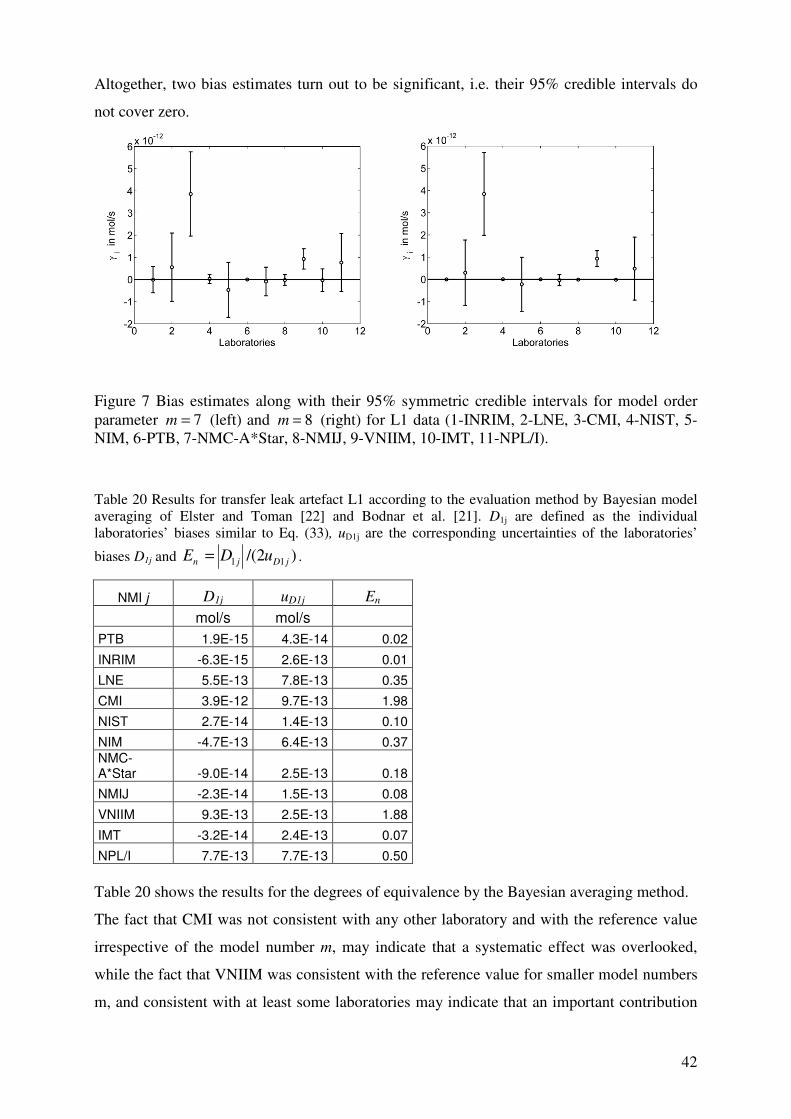
42

Altogether, two bias estimates turn out to be significant, i.e. their 95% credible intervals do

not cover zero.

Figure 7 Bias estimates along with their 95% symmetric credible intervals for model order parameter 7=m (left) and 8=m (right) for L1 data (1-INRIM, 2-LNE, 3-CMI, 4-NIST, 5-NIM, 6-PTB, 7-NMC-A*Star, 8-NMIJ, 9-VNIIM, 10-IMT, 11-NPL/I).

Table 20 Results for transfer leak artefact L1 according to the evaluation method by Bayesian model averaging of Elster and Toman [22] and Bodnar et al. [21]. D1j are defined as the individual laboratories’ biases similar to Eq. (33), uD1j are the corresponding uncertainties of the laboratories’

biases D1j and )2/( 11 jDjn uDE = .

NMI j D1j uD1j En

mol/s mol/s

PTB 1.9E-15 4.3E-14 0.02

INRIM -6.3E-15 2.6E-13 0.01

LNE 5.5E-13 7.8E-13 0.35

CMI 3.9E-12 9.7E-13 1.98

NIST 2.7E-14 1.4E-13 0.10

NIM -4.7E-13 6.4E-13 0.37

NMC-A*Star -9.0E-14 2.5E-13 0.18

NMIJ -2.3E-14 1.5E-13 0.08

VNIIM 9.3E-13 2.5E-13 1.88

IMT -3.2E-14 2.4E-13 0.07

NPL/I 7.7E-13 7.7E-13 0.50

Table 20 shows the results for the degrees of equivalence by the Bayesian averaging method.

The fact that CMI was not consistent with any other laboratory and with the reference value

irrespective of the model number m, may indicate that a systematic effect was overlooked,

while the fact that VNIIM was consistent with the reference value for smaller model numbers

m, and consistent with at least some laboratories may indicate that an important contribution

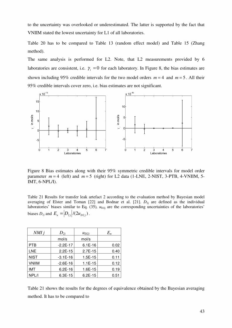
43

to the uncertainty was overlooked or underestimated. The latter is supported by the fact that

VNIIM stated the lowest uncertainty for L1 of all laboratories.

Table 20 has to be compared to Table 13 (random effect model) and Table 15 (Zhang

method).

The same analysis is performed for L2. Note, that L2 measurements provided by 6

laboratories are consistent, i.e. 0=iγ for each laboratory. In Figure 8, the bias estimates are

shown including 95% credible intervals for the two model orders 4=m and 5=m . All their

95% credible intervals cover zero, i.e. bias estimates are not significant.

Figure 8 Bias estimates along with their 95% symmetric credible intervals for model order parameter 4=m (left) and 5=m (right) for L2 data (1-LNE, 2-NIST, 3-PTB, 4-VNIIM, 5-IMT, 6-NPL/I).

Table 21 Results for transfer leak artefact 2 according to the evaluation method by Bayesian model averaging of Elster and Toman [22] and Bodnar et al. [21]. D2j are defined as the individual laboratories’ biases similar to Eq. (35), uD2j are the corresponding uncertainties of the laboratories’

biases D1j and )2/( 22 jDjn uDE = .

NMI j D2j uD2j En

mol/s mol/s

PTB -2.2E-17 6.1E-16 0.02

LNE 2.2E-15 2.7E-15 0.40

NIST -3.1E-16 1.5E-15 0.11

VNIIM -2.6E-16 1.1E-15 0.12

IMT 6.2E-16 1.6E-15 0.19

NPL/I 6.3E-15 6.2E-15 0.51

Table 21 shows the results for the degrees of equivalence obtained by the Bayesian averaging

method. It has to be compared to

44

Table 14 (random effect model) and Table 19 (Zhang method).

Another result obtained is the probability density function ),,|( muxp β for the rate of change

β of the measurand which is shown in Figure 9. As most of the probability measure lies

below zero, a negative change in time of the measurand is suggested. In Sections 9.2 and 13.1

we found 1310)92.057.7( −⋅±−=β (mol/s)/a (Eq. (24)) and 1310)63.061.7( −⋅±−=β

(mol/s)/a, respectively, by least-squares fit to the pilot laboratory data. These values lie very

close to the peak of the density function and are in full agreement with this result.

Figure 9 Distribution for the rate of change β for L1 data obtained for model order parameter 7=m .

Analogously, we analyse the data for L2. In Figure 10 the density ),,|( muxp β is shown. For

L2 we have the consistency of all measurements that motivates the choice of 6== pm and

model order m = 4. In this figure we also observe that most of the probability measure is

concentrated below zero which suggests that a real (negative) change of the measurand was

present. In Sections 9.2 and 13.1 we found 1510)06.165.1( −⋅±−=β (mol/s)/a (Eq.(28)) and

1510)25.066.1( −⋅±−=β (mol/s)/a, respectively, by least-squares fit to the pilot laboratory

data. As for L1, these values lie very close to the peak of the density function and are in full

agreement with this result.

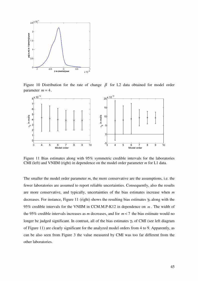
45

Figure 10 Distribution for the rate of change β for L2 data obtained for model order parameter 4=m .

Figure 11 Bias estimates along with 95% symmetric credible intervals for the laboratories CMI (left) and VNIIM (right) in dependence on the model order parameter m for L1 data.

The smaller the model order parameter m, the more conservative are the assumptions, i.e. the

fewer laboratories are assumed to report reliable uncertainties. Consequently, also the results

are more conservative, and typically, uncertainties of the bias estimates increase when m

decreases. For instance, Figure 11 (right) shows the resulting bias estimates γ9 along with the

95% credible intervals for the VNIIM in CCM.M.P-K12 in dependence on m . The width of

the 95% credible intervals increases as m decreases, and for 7<m the bias estimate would no

longer be judged significant. In contrast, all of the bias estimates γ3 of CMI (see left diagram

of Figure 11) are clearly significant for the analyzed model orders from 4 to 9. Apparently, as

can be also seen from Figure 3 the value measured by CMI was too far different from the

other laboratories.

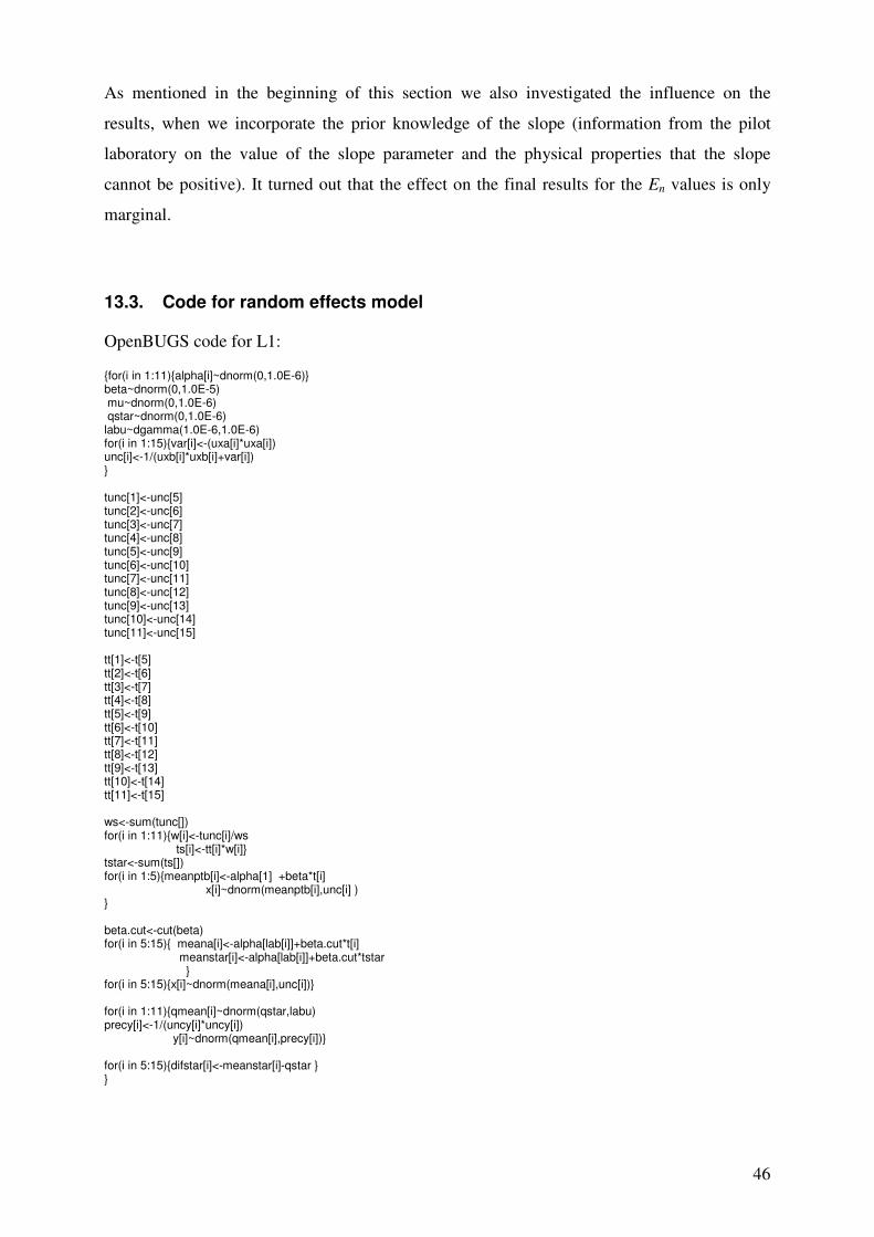
46

As mentioned in the beginning of this section we also investigated the influence on the

results, when we incorporate the prior knowledge of the slope (information from the pilot

laboratory on the value of the slope parameter and the physical properties that the slope

cannot be positive). It turned out that the effect on the final results for the En values is only

marginal.

13.3. Code for random effects model

OpenBUGS code for L1:

{for(i in 1:11){alpha[i]~dnorm(0,1.0E-6)} beta~dnorm(0,1.0E-5) mu~dnorm(0,1.0E-6) qstar~dnorm(0,1.0E-6) labu~dgamma(1.0E-6,1.0E-6) for(i in 1:15){var[i]<-(uxa[i]*uxa[i]) unc[i]<-1/(uxb[i]*uxb[i]+var[i]) } tunc[1]<-unc[5] tunc[2]<-unc[6] tunc[3]<-unc[7] tunc[4]<-unc[8] tunc[5]<-unc[9] tunc[6]<-unc[10] tunc[7]<-unc[11] tunc[8]<-unc[12] tunc[9]<-unc[13] tunc[10]<-unc[14] tunc[11]<-unc[15] tt[1]<-t[5] tt[2]<-t[6] tt[3]<-t[7] tt[4]<-t[8] tt[5]<-t[9] tt[6]<-t[10] tt[7]<-t[11] tt[8]<-t[12] tt[9]<-t[13] tt[10]<-t[14] tt[11]<-t[15] ws<-sum(tunc[]) for(i in 1:11){w[i]<-tunc[i]/ws ts[i]<-tt[i]*w[i]} tstar<-sum(ts[]) for(i in 1:5){meanptb[i]<-alpha[1] +beta*t[i] x[i]~dnorm(meanptb[i],unc[i] ) } beta.cut<-cut(beta) for(i in 5:15){ meana[i]<-alpha[lab[i]]+beta.cut*t[i] meanstar[i]<-alpha[lab[i]]+beta.cut*tstar } for(i in 5:15){x[i]~dnorm(meana[i],unc[i])} for(i in 1:11){qmean[i]~dnorm(qstar,labu) precy[i]<-1/(uncy[i]*uncy[i]) y[i]~dnorm(qmean[i],precy[i])} for(i in 5:15){difstar[i]<-meanstar[i]-qstar } }

47

Initial values: list(mu=0, labu=1)

Data for L1: list(x=c(4.398,4.354,4.29,4.27,4.424,4.397,4.509,4.776,4.379,4.263,4.300,4.305,4.411,4.300,4.407),uxa=c(0.0076,0.015,0.012, 0.0051,0.012,0.015,0.0051,0.043,0.0052,0.0086,0.03,0.00076,0.0056,0.0062,0.022),uxb=c(0.013,0.013,0.013,0.013,0.014,0.073,0.059,0.081,0.017,0.051,0.015,0.043,0.011,0.015,0.048),t=c(151,376,622,769,0,40,55,109,222,260,335,439,520,607,676), lab=c(1,1,1,1,1,2,3,4,5,6,7,8,9,10,11),y=c(4.35,4.33,4.45,4.72,4.35,4.24,4.29,4.32,4.45,4.35,4.47),uncy=c(0.02,0.09,0.069,0.11,0.034,0.063,0.094,0.047,0.035,0.039,0.069))

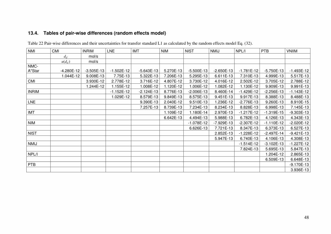
48

13.4. Tables of pair-wise differences (random effects model)

Table 22 Pair-wise differences and their uncertainties for transfer standard L1 as calculated by the random effects model Eq. (32).

NMI CMI INRIM LNE IMT NIM NIST NMIJ NPL/I PTB VNIIM

djj' mol/s

u(djj') mol/s

NMC-A*Star -4.280E-12 -3.505E-13 -1.502E-12 -5.643E-13 5.270E-13 -5.500E-13 -2.650E-13 -1.781E-12 -5.750E-13 -1.493E-12

1.044E-12 9.008E-13 7.75E-13 5.322E-13 7.206E-13 5.295E-13 6.611E-13 7.310E-13 4.999E-13 5.517E-13

CMI 3.930E-12 2.778E-12 3.716E-12 4.807E-12 3.730E-12 4.016E-12 2.502E-12 3.705E-12 2.788E-12

1.244E-12 1.155E-12 1.008E-12 1.120E-12 1.006E-12 1.082E-12 1.130E-12 9.909E-13 9.991E-13

INRIM -1.152E-12 -2.124E-13 8.776E-13 -2.006E-13 8.460E-14 -1.429E-12 -2.256E-13 -1.143E-12

1.029E-12 8.579E-13 9.849E-13 8.575E-13 9.451E-13 9.917E-13 8.388E-13 8.488E-13

LNE 9.390E-13 2.040E-12 9.510E-13 1.236E-12 -2.776E-13 9.260E-13 8.910E-15

7.257E-13 8.739E-13 7.234E-13 8.234E-13 8.828E-13 6.998E-13 7.145E-13

IMT 1.109E-12 1.180E-14 2.970E-13 -1.217E-12 -1.319E-15 -9.303E-13

6.642E-13 4.494E-13 5.988E-13 6.782E-13 4.126E-13 4.343E-13

NIM -1.078E-12 -7.929E-13 -2.307E-12 -1.110E-12 -2.020E-12

6.626E-13 7.721E-13 8.347E-13 6.373E-13 6.527E-13

NIST 2.852E-13 -1.228E-12 -2.497E-14 -9.421E-13

5.947E-13 6.740E-13 4.106E-13 4.308E-13

NMIJ -1.514E-12 -3.102E-13 -1.227E-12

7.824E-13 5.695E-13 5.847E-13

NPL/I 1.204E-12 2.865E-13

6.509E-13 6.648E-13

PTB -9.170E-13

3.936E-13

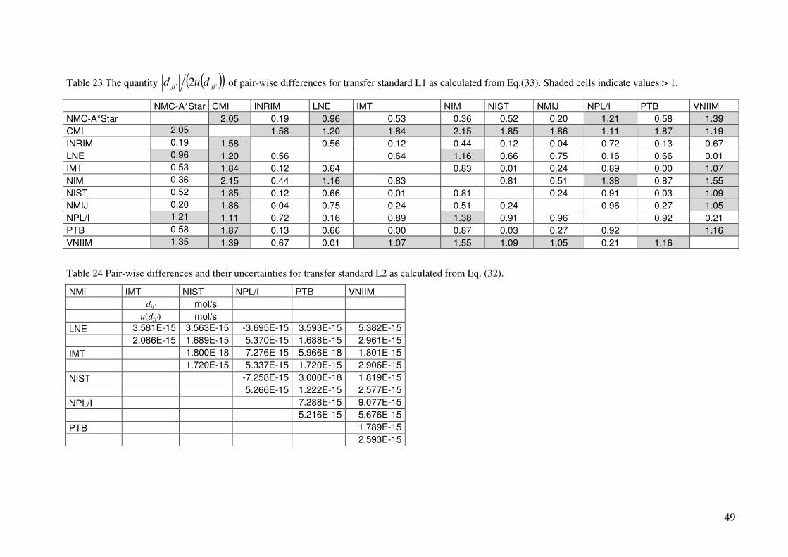
49

Table 23 The quantity ( )( )'' 2 jjjj dud of pair-wise differences for transfer standard L1 as calculated from Eq.(33). Shaded cells indicate values > 1.

NMC-A*Star CMI INRIM LNE IMT NIM NIST NMIJ NPL/I PTB VNIIM

NMC-A*Star 2.05 0.19 0.96 0.53 0.36 0.52 0.20 1.21 0.58 1.39

CMI 2.05 1.58 1.20 1.84 2.15 1.85 1.86 1.11 1.87 1.19

INRIM 0.19 1.58 0.56 0.12 0.44 0.12 0.04 0.72 0.13 0.67

LNE 0.96 1.20 0.56 0.64 1.16 0.66 0.75 0.16 0.66 0.01

IMT 0.53 1.84 0.12 0.64 0.83 0.01 0.24 0.89 0.00 1.07

NIM 0.36 2.15 0.44 1.16 0.83 0.81 0.51 1.38 0.87 1.55

NIST 0.52 1.85 0.12 0.66 0.01 0.81 0.24 0.91 0.03 1.09

NMIJ 0.20 1.86 0.04 0.75 0.24 0.51 0.24 0.96 0.27 1.05

NPL/I 1.21 1.11 0.72 0.16 0.89 1.38 0.91 0.96 0.92 0.21

PTB 0.58 1.87 0.13 0.66 0.00 0.87 0.03 0.27 0.92 1.16

VNIIM 1.35 1.39 0.67 0.01 1.07 1.55 1.09 1.05 0.21 1.16

Table 24 Pair-wise differences and their uncertainties for transfer standard L2 as calculated from Eq. (32).

NMI IMT NIST NPL/I PTB VNIIM

djj' mol/s

u(djj') mol/s

LNE 3.581E-15 3.563E-15 -3.695E-15 3.593E-15 5.382E-15

2.086E-15 1.689E-15 5.370E-15 1.688E-15 2.961E-15

IMT -1.800E-18 -7.276E-15 5.966E-18 1.801E-15

1.720E-15 5.337E-15 1.720E-15 2.906E-15

NIST -7.258E-15 3.000E-18 1.819E-15

5.266E-15 1.222E-15 2.577E-15

NPL/I 7.288E-15 9.077E-15

5.216E-15 5.676E-15

PTB 1.789E-15

2.593E-15

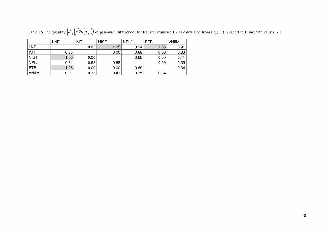
50

Table 25 The quantity ( )( )'' 2 jjjj dud of pair-wise differences for transfer standard L2 as calculated from Eq.(33). Shaded cells indicate values > 1.

LNE IMT NIST NPL/I PTB VNIIM

LNE 0.85 1.05 0.34 1.06 0.91

IMT 0.85 0.00 0.68 0.00 0.33

NIST 1.05 0.00 0.68 0.00 0.41

NPL/I 0.34 0.68 0.68 0.69 0.35

PTB 1.06 0.00 0.00 0.69 0.34

VNIIM 0.91 0.33 0.41 0.35 0.34

Documents

Final report of key comparison CCM.P-K12 for very low ... in this report, ... comparison of flow rates of helium leak artefacts (leak rates) ... test leak at 23.0°C. (1)Published