University of California, San Diego UCSD-CER-09-02

Center for Energy Research University of California, San Diego 9500 Gilman Drive La Jolla, CA 92093-0417

High temperature liquid metal loop – Final report –

J. Stromsoe

May 2009

  

High Temperature Liquid Metal Loop   Final Report 

 J. Stromsoe 

 Center for Energy Research 

University of California, San Diego 9500 Gilman Dr. 92093‐0411 

 

2

Contents: 

I. Introduction/History a. Past Experimentation 

i. PICOLO Loop, Germany ii. CORRIDA Loop (Karlsruhe Lead Laboratory, KALLA), Germany iii. ITER TBM (test blanket module, designed by FZK) iv. Flow Channel Inserts (Germany) v. Bruce Pint, ORNL 

b. Research Possibilties i. Loop Requirements 

1. Testing 2. Safety 3. Limitations 

c. Project Scope II. Conceptual Design 

a. High Temperature Loop Components i. Heat Exchanger  ii. Liquid Metal pump iii. Heater 

III. Preliminary Design a. High Temperature Loop Components 

i. Heat Exchanger Configuration Selection ii. Concentric Tube Heat Exchanger Model and Heater Application 

1. Abstract 2. Assumptions 3. Dimensions 4. Properties 5. Theory 6. Results 7. Discussion 8. Cost/Manufacture 

iii. High Temperature Pumping Components 1. AC Coil Pump 2. Permanent Magnet Pump 

IV. Conclusions V. References 

 

 

3

I. Introduction 

  In order to provide UCSD with a high temperature liquid metal loop which would have a 

unique capability for high temperature compatibility testing, a literature review was conducted 

to consider each of the already tested possibilities, and to see where new challenges and 

promising technologies in this field lie.  This would help determine the focus of the project to 

ensure maximum scientific and engineering value of the final results determined by the 

experiments performed with the high temperature loop.  The literature study conducted here, 

by considering what has already been accomplished in the past, will shed some light on what 

we at UCSD would like to accomplish, and what the implications of our findings would mean for 

the future of structural materials used in liquid metal blanket designs for fusion and possibly 

generation IV fission reactors.  

   Liquid metals have surfaced as a useful tool in harnessing the energy from nuclear 

reactors by trapping the heat produced and transporting it to be converted into electrical 

energy.  Unfortunately, liquid metals are often incompatible with structural materials needed 

to support the weight of the liquid metal blanket.  Loop tests on various eutectics including 

Lead, Sodium, Lead‐Bismuth (LBE), Lithium, and Lead Lithium have all been completed using 

mainly ferritic steels or stainless steel as test material, subjected to either a forced or natural 

convective flow of the liquid metal.  Corrosion of steels is an inevitable [1] problem in most 

liquid flows being considered for use in liquid metal blanket design, and must be addressed to 

ensure a respectable reactor lifetime.  Tests on silicon carbide have been performed as well in 

flowing liquid metals, but to a much lesser extent.  Therefore, much of the literature review will 

4

focus on SiC.  Here the experiments from other loops around the world will be considered in 

the light of a new innovative loop to be designed and built by CER at UCSD. 

 

a) Past Experimentation  

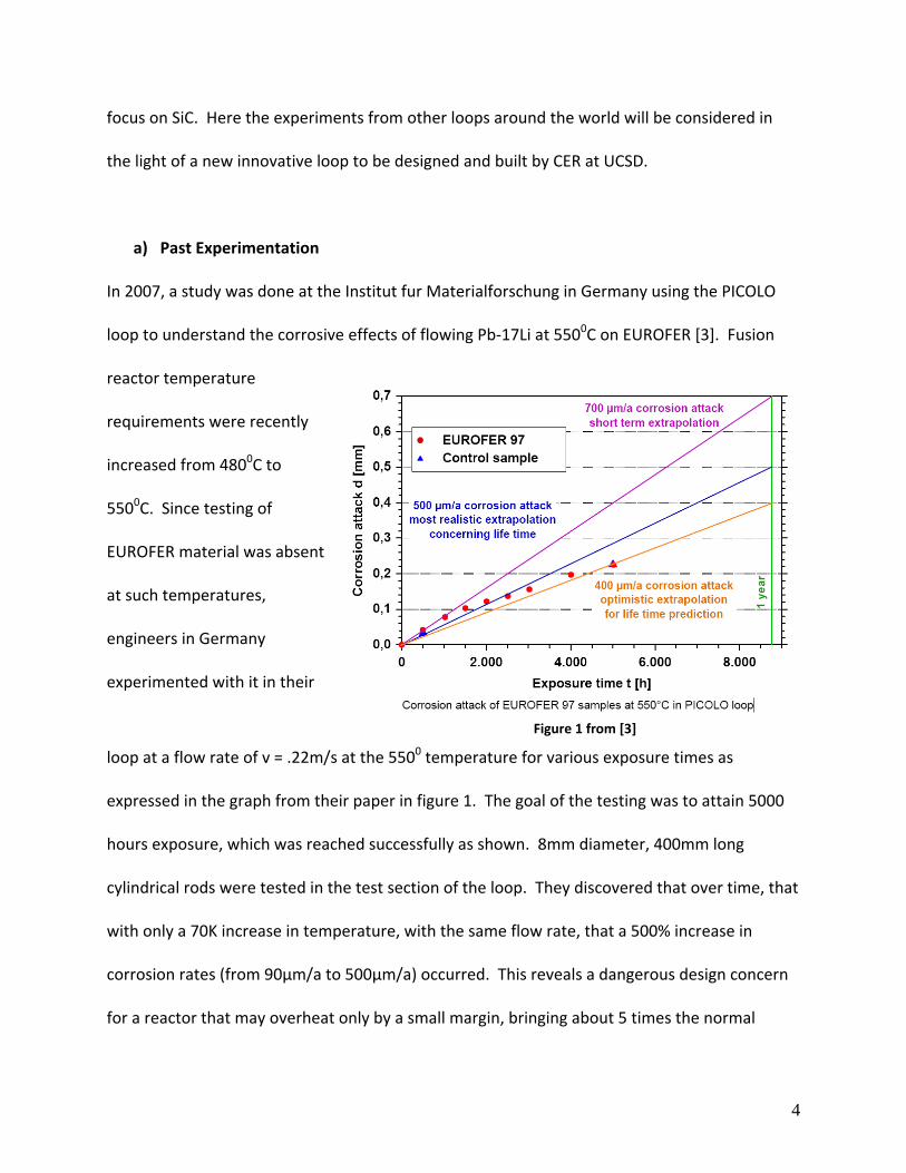
In 2007, a study was done at the Institut fur Materialforschung in Germany using the PICOLO 

loop to understand the corrosive effects of flowing Pb‐17Li at 5500C on EUROFER [3].  Fusion 

reactor temperature 

requirements were recently 

increased from 4800C to 

5500C.  Since testing of 

EUROFER material was absent 

at such temperatures, 

engineers in Germany 

experimented with it in their 

loop at a flow rate of v = .22m/s at the 5500 temperature for various exposure times as 

expressed in the graph from their paper in figure 1.  The goal of the testing was to attain 5000 

hours exposure, which was reached successfully as shown.  8mm diameter, 400mm long 

cylindrical rods were tested in the test section of the loop.  They discovered that over time, that 

with only a 70K increase in temperature, with the same flow rate, that a 500% increase in 

corrosion rates (from 90µm/a to 500µm/a) occurred.  This reveals a dangerous design concern 

for a reactor that may overheat only by a small margin, bringing about 5 times the normal 

Figure 1 from [3] 

5

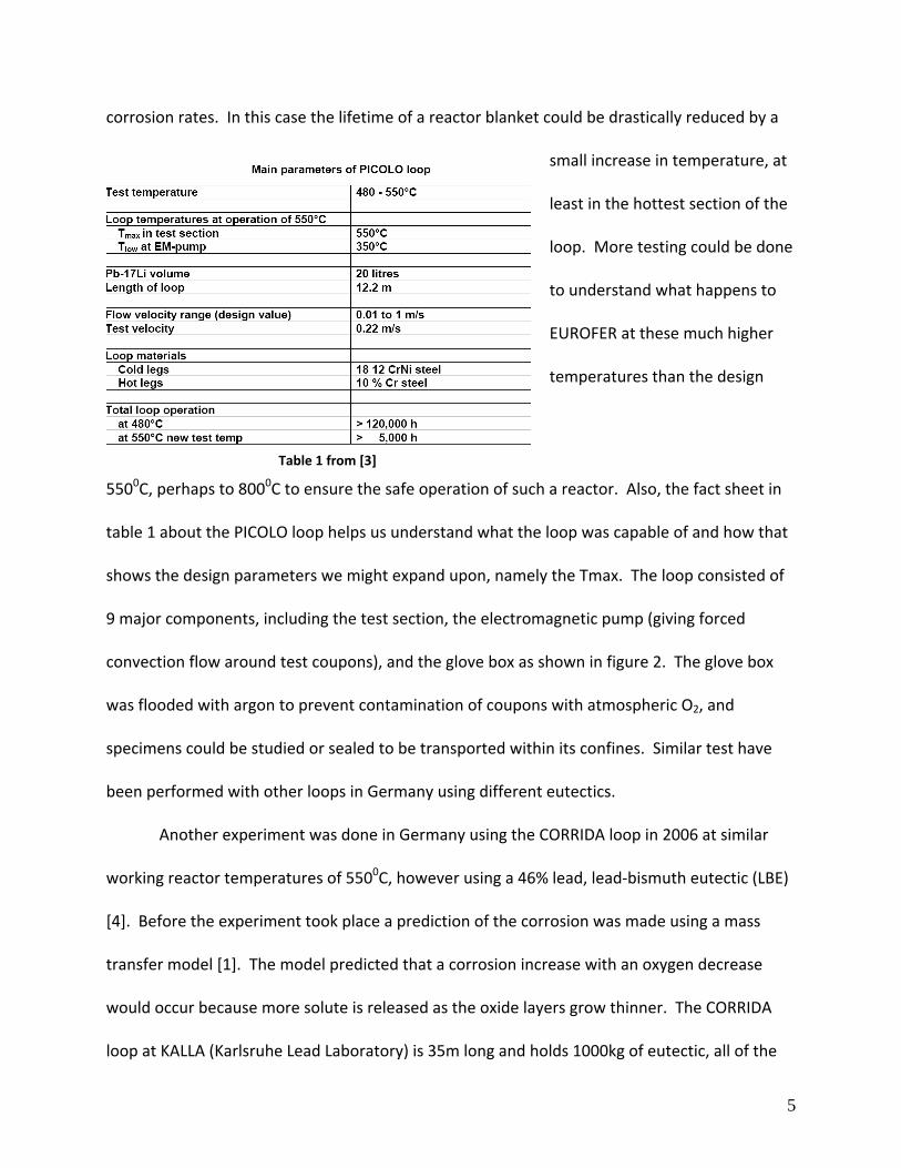
corrosion rates.  In this case the lifetime of a reactor blanket could be drastically reduced by a 

small increase in temperature, at 

least in the hottest section of the 

loop.  More testing could be done 

to understand what happens to 

EUROFER at these much higher 

temperatures than the design 

5500C, perhaps to 8000C to ensure the safe operation of such a reactor.  Also, the fact sheet in 

table 1 about the PICOLO loop helps us understand what the loop was capable of and how that 

shows the design parameters we might expand upon, namely the Tmax.  The loop consisted of 

9 major components, including the test section, the electromagnetic pump (giving forced 

convection flow around test coupons), and the glove box as shown in figure 2.  The glove box 

was flooded with argon to prevent contamination of coupons with atmospheric O2, and 

specimens could be studied or sealed to be transported within its confines.  Similar test have 

been performed with other loops in Germany using different eutectics. 

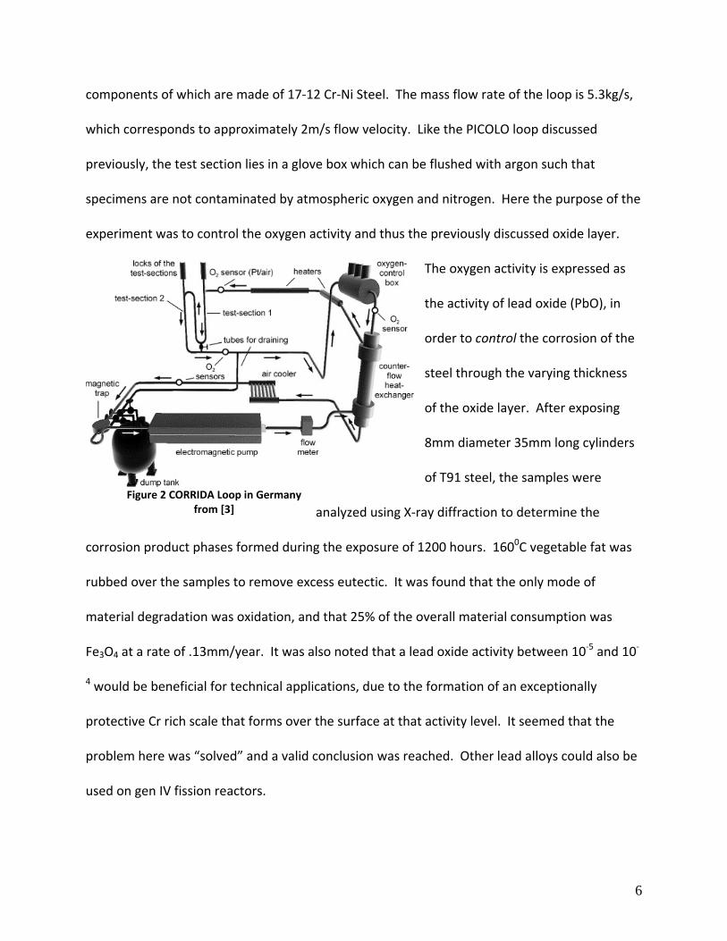
  Another experiment was done in Germany using the CORRIDA loop in 2006 at similar 

working reactor temperatures of 5500C, however using a 46% lead, lead‐bismuth eutectic (LBE) 

[4].  Before the experiment took place a prediction of the corrosion was made using a mass 

transfer model [1].  The model predicted that a corrosion increase with an oxygen decrease 

would occur because more solute is released as the oxide layers grow thinner.  The CORRIDA 

loop at KALLA (Karlsruhe Lead Laboratory) is 35m long and holds 1000kg of eutectic, all of the 

Table 1 from [3]

6

components of which are made of 17‐12 Cr‐Ni Steel.  The mass flow rate of the loop is 5.3kg/s, 

which corresponds to approximately 2m/s flow velocity.  Like the PICOLO loop discussed 

previously, the test section lies in a glove box which can be flushed with argon such that 

specimens are not contaminated by atmospheric oxygen and nitrogen.  Here the purpose of the 

experiment was to control the oxygen activity and thus the previously discussed oxide layer.  

The oxygen activity is expressed as 

the activity of lead oxide (PbO), in 

order to control the corrosion of the 

steel through the varying thickness 

of the oxide layer.  After exposing 

8mm diameter 35mm long cylinders 

of T91 steel, the samples were 

analyzed using X‐ray diffraction to determine the 

corrosion product phases formed during the exposure of 1200 hours.  1600C vegetable fat was 

rubbed over the samples to remove excess eutectic.  It was found that the only mode of 

material degradation was oxidation, and that 25% of the overall material consumption was 

Fe3O4 at a rate of .13mm/year.  It was also noted that a lead oxide activity between 10‐5 and 10‐

4 would be beneficial for technical applications, due to the formation of an exceptionally 

protective Cr rich scale that forms over the surface at that activity level.  It seemed that the 

problem here was “solved” and a valid conclusion was reached.  Other lead alloys could also be 

used on gen IV fission reactors. 

Figure 2 CORRIDA Loop in Germanyfrom [3] 

7

  The U.S. Department of Energy is interested in developing the gen IV nuclear reactor for 

use in the US by 2020.  In response to this, several entities including MIT, Idaho National 

Engineering and Environmental Laboratory, Los Alamos National Laboratory, and quite a few 

others began testing lead alloy coolants, namely lead bismuth.  It has been pointed out, [5] that 

lead alloys are now being reconsidered for use in nuclear fission reactors because of their 

inertness to water and air, unlike sodium,  as well as its better shielding against gamma rays, 

higher boiling temperature than sodium, and successful tests on a smaller scale (the Alpha class 

Russian submarines).   

  What is lacking in the LBE case is testing on natural and forced convection to determine 

the heat transfer and natural circulation characteristics on a more full scale [5].  While it is 

rather difficult to fabricate a blanket structure in a laboratory setting for testing, even on a 

smaller scale, corrosion has been the main issue with LBE since 1950, and still today is one of 

the fundamental problems facing the advancement of the gen IV reactor.  More specifically, 

dissolution of the blanket wall in hot regions and precipitation in the high hot‐to‐cold gradient 

zones causes blockage of components such as heat exchangers [5, 615‐616] especially with 

steel.  It is also pointed out that adding Zr, Tn, and Cr to the coolant itself or adding surface 

coatings like Al, Mo, Zr, or SiC on metal surfaces greatly reduce corrosion, however erratic 

adherence to the surface has been a problem, and irregularities on the surface tend to corrode 

more readily.  Each of these solutions has not been fully explored. 

  Moving into the lithium lead eutectic, the following were found [6] to be compatible in a 

static environment: ZrC, TiN, MgO, and SiC.  Lithium lead was first considered because it is able 

to both breed tritium and act as a coolant.  In the study performed [6], the lithium lead eutectic 

8

was made out of 99.26% Pb and .74% Li.  1”x 1” squares of SiC A were prepared using SiC cloth 

as the fiber and chemically vapor deposited SiC as the matrix.  It yielded a composite that was 

85% of the density of the theoretical value.  These tests were static, and simply done in Mo 

containers at 1073K.  After 1500 hours, the samples were reviewed using a scanning electron 

microscope.  Each was found to qualitatively have “no reaction” as the only observation, 

revealing that the study was done rather simplistically.  While conducted at a high temperature, 

the eutectic was not flowing over the specimens, so the results are questionable as far as their 

implications in the use of composites in a true reactor.  Also, for fusion reactors, 83% lead with 

17% lithium will be used, which poses more of a corrosion problem since the corrosion 

(especially with steels) is mainly associated with the activity of lithium.  

  Despite the previous results, in 1995 the water cooled Pb‐17Li (Water Cooled Lead 

Lithium or WCLL) DEMO breeding blanket was selected for further study [7] for a testing 

representation module in ITER.  The proposal desired that the blanket have a lifetime of 20,000 

hours and an outlet temperature of 3250C, using a structural material of martensitic steel 

(considered for design purposes only, because corrosion has not been solved).  Work has begun 

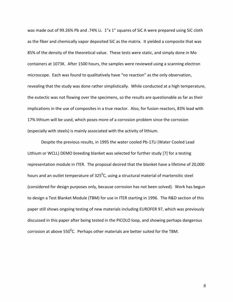
to design a Test Blanket Module (TBM) for use in ITER starting in 1996.  The R&D section of this 

paper still shows ongoing testing of new materials including EUROFER 97, which was previously 

discussed in this paper after being tested in the PICOLO loop, and showing perhaps dangerous 

corrosion at above 5500C.  Perhaps other materials are better suited for the TBM. 

9

Figure 3 from Institute for Reactor Safety a TBM concept for ITER insertion designed by Forschungszentrum Karlsruhe, in Germany 

 

Another proposal later, by one of the same researchers from the WCLL TBM proposal 

came up with a helium cooled (HCLL) proposal as well for lead lithium [8].  The paper merely 

showed that the “Integral TBM” one of four designs, would be implemented in the high‐duty D‐

T phase of ITER to demonstrate a reliable and controllable mock up of a HCLL device.  No design 

elements were disclosed in the document, unfortunately.  A few researchers from Germany, 

however, did have some design ideas for how an advanced lead lithium blanket might be 

designed.  

10

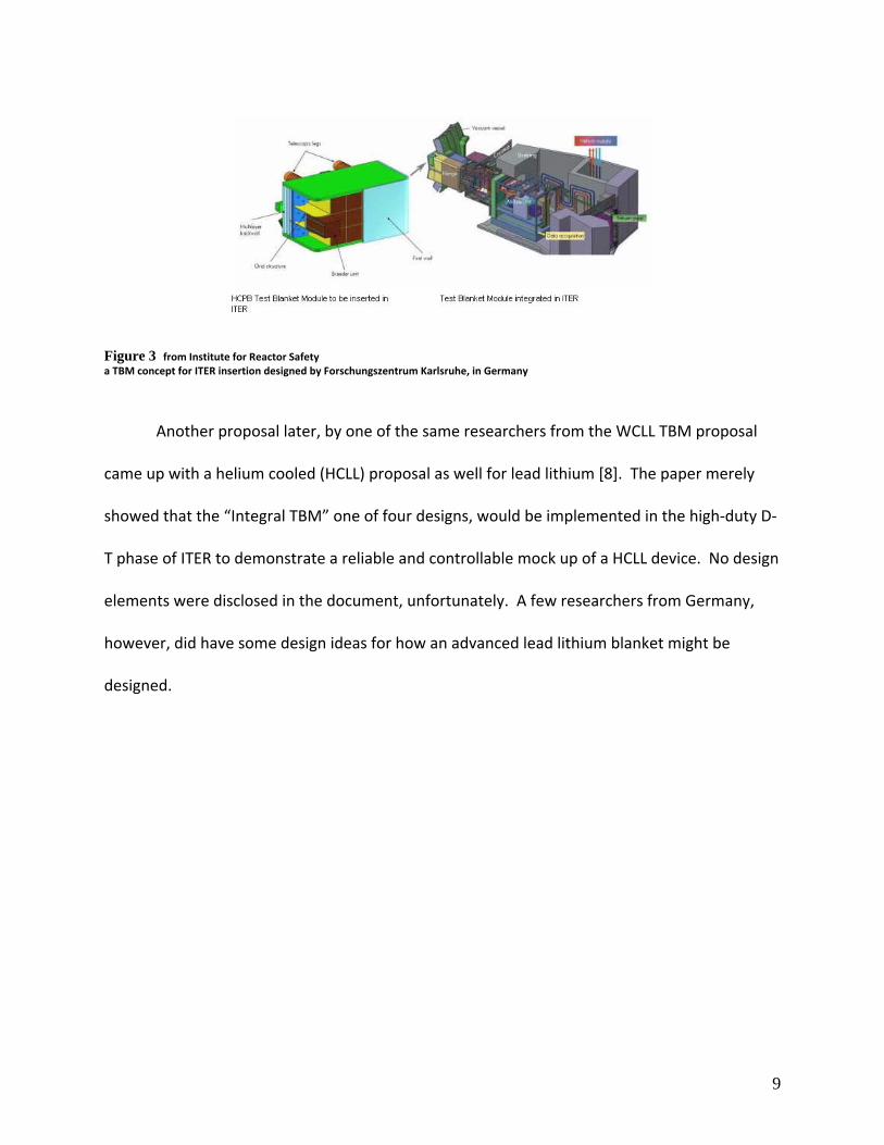
  These researchers felt that SiC could be used as an insert in the lead lithium channels, 

utilizing the steel as a structural 

element for the wall, while merely using 

the brittle SiC as corrosion shielding.  

They came up with a conceptual design 

[2] that was planned for launch in 2001 

within the EU fusion program.  These 

inserts would allow for a high outlet 

temperature for the lead lithium, 

increasing the efficiency of a power 

conversion system.  The reason SiC seems like such an attractive solution is due to the 

approximately 7 Tesla magnetic field  present in the blanket region, which would require 

electrical insulation from the first wall structure.  The proposal consists of adding 5mm thick 

inserts into the flow channels.  The only question is compatibility of SiC with lithium lead.  The 

study uses [6] as a reference to show that it is in fact compatible at up to 8000C.  Keeping in 

mind that the study done in [6] was a static fluid experiment with a different % of lithium to 

lead, more quantitative testing is necessary to show that it is compatible in flowing lead lithium, 

and what modes of mass transfer come into play.  

  Some laboratory results have determined that thermally grown Alumina on a small 

piece of “commercial steel” has abnormally large grain growth after being exposed to 8000C 

lead lithium for 1000 hours [9].  It seems that this solution, a layer of aluminum oxide, seems to 

be questionable as well as untested fully. 

Figure 4 Sectioned view of Helium Cooled Blanket with Flowing Lithium Lead as well as 5mm SiC Inserts, From [2] 

11

b) Research Possibilities 

  From the literature review conducted, it seems that the two viable solutions for future 

fusion and/or fission reactors are either lead lithium or lead bismuth coolants.  While steel and 

EUROFER have been well tested, SiC inserts, nor any other electrically thermally insulating 

composite has been tested.  This could make composites a starting point for the liquid metal 

loop design at UCSD.   

  To test steel in a loop, the main concern is with the control of lead oxide in the liquid 

metal, requiring 02 sensors, and other equipment.  It seems that the loop could be later 

upgraded to perform such a task, but could be constructed mainly to test composite material.  

Also, it would seem superfluous to test steels for oxidation rates based on the activity of lead 

oxide in the coolant since it has been done already in [3] [1]. 

  Of course, something that not many others have done is sample the lead lithium in the 

loop and chemically analyze it for concentrations of ceramic material, and in this sense gauge 

the ill‐effects of corrosion on system components (i.e. clogging) like counter‐flow heat 

exchangers.  While corrosion of SiC would be the main focus, the analysis of the coolant itself 

seems a necessary task and a method for doing so will need to be developed. 

  SiC coupons could easily be tested in the same manner which laser struck coupons are 

currently examined, with an SEM.  This would be necessary to see the grain size and material 

loss of each specimen.  Also, an accurate weighing of each SiC specimen would be difficult to 

determine due to the porous qualities of a composite.  Thus this method would also need to be 

devised.   

12

  Material standards would also need to be set both for lead lithium eutectic (or possibly 

lead bismuth) as well as for SiC.  Since EUROFER has its own standards, we would merely need 

to verify these.  A technique for making SiC test coupons would also need to be defined.  Tests 

of at least up to 5000 hours should be conducted, but I would like the UCSD loop to at least 

reach 15000 hours of continuous operation, which is undocumented currently.  

  The loop design itself should start very simply to ensure ease of manufacture and 

accuracy of initial results.  Once the loop is proven, further upgrades could be added to enable 

the additions of different types of coupons (i.e. EUROFER 97, Alumina coated steels), as well as 

other types of equipment (electromagnetic pumps, upgraded heaters/heat exchangers, ect…).  

Starting simply is the key.   

Also, heavy safety measures will have to be implemented.  A loop designed to run for 

thousands of hours unattended must have an alarm linked to security or police in case of 

malfunction or natural disaster.  Before deciding detailed parameters and components of the 

loop itself, I’d like the opportunity to work on an already established loop and completely 

understand its operation.   

  Detailed CAD drawings and thermodynamic programming will be necessary to make 

sure that the loop is manufactured correctly and efficiently and that each component is capable 

of the tasks we need it to perform.  Thermodynamic programming could be done by hand 

through MATLAB or a similar compiler, or it could be accomplished through the use of a 

commercially available program.  Extensive hand calculations will need to be performed to 

ensure the accuracy of the program.   

13

  At this point labor time and costs are difficult to estimate.  It depends on material cost, 

component (heaters/exchangers) costs, hours of labor involved, safety training, tools, software 

ect…  These are just some of the costs associated with the project; an ongoing cost analysis 

before the time of construction will be necessary to remain within budget boundaries.  

   

c) Project Scope 

  If these tests are successful, it could lead to a more immediate advance in fusion reactor 

design.  The coolant liquid metal blanket is essentially the method by which we are able to 

attain energy from a fusion or fission reaction.  Without a suitable blanket wall material, the 

process for developing these reactors will be hindered.  Developing this unique capability for 

testing at UCSD will shed some light on this age old problem of corrosion with liquid metals.  

  This may also open the doors for UCSD to work with engineers/physicists from other 

universities and allow for collaboration efforts that otherwise would not have occurred.  These 

sort of relationships would also open the doors for others students and faculty to gain new 

knowledge and ideas. 

  The results of such a project could lead to the fabrication of a Test Blanket Module 

(TBM) made by UCSD which would be of use in ITER.  I believe such results would be innovative 

and if ITER tests are successful, a breakthrough in corrosion for this application.   

 

 

 

 

14

II. Conceptual Design 

  To narrow the many ideas behind each of the components of the high temperature loop at 

UCSD, a conceptual design study was conducted.  This allows the determination of which types of loop 

components should be focused upon and studied with greater detail and modeling.    

a) High Temperature Components 

  The three major loop components which must be carefully reviewed given the high 

temperatures involved in the experiments are the heater, the heat exchanger, and the 

electromagnetic pump.  The loop must be designed around these key components in order to 

keep the test section at the temperatures and flow rates desired.  Design parameters such as 

performance, cost, and ease of manufacture were taken into consideration in the following 

trade studies. 

i) Heat Exchanger 

  The heat exchanger was considered first in the design of a high temperature loop since 

the overall performance of the exchanger dictates the amount of heating necessary to maintain 

the test section temperature.  Two types of exchanger configurations were considered based 

upon available high temperature materials including a counterflow and shell‐and‐tube with 

multiple passes.   Each configuration has potential strengths and weaknesses.  The following 

figure of merit chart describes these.  The scale is from 0 to 5, 5 being the best, 0 being the 

worst. 

 

 

 

15

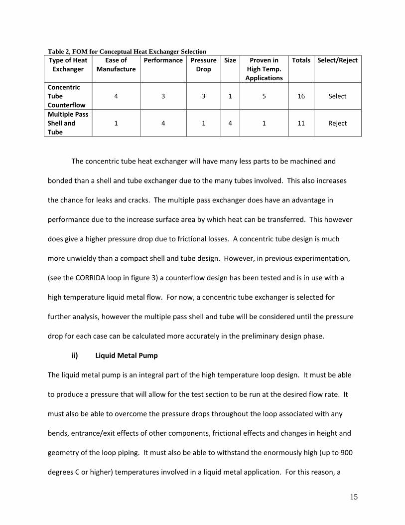
Table 2, FOM for Conceptual Heat Exchanger Selection Type of Heat Exchanger 

Ease of Manufacture 

Performance Pressure Drop 

Size Proven in High Temp. Applications 

Totals  Select/Reject

Concentric Tube Counterflow 

 4 

 3 

 3 

 1 

 5 

 16 

 Select 

Multiple Pass Shell and Tube 

 1 

 4 

 1 

 4 

 1 

 11 

 Reject 

 

  The concentric tube heat exchanger will have many less parts to be machined and 

bonded than a shell and tube exchanger due to the many tubes involved.  This also increases 

the chance for leaks and cracks.  The multiple pass exchanger does have an advantage in 

performance due to the increase surface area by which heat can be transferred.  This however 

does give a higher pressure drop due to frictional losses.  A concentric tube design is much 

more unwieldy than a compact shell and tube design.  However, in previous experimentation, 

(see the CORRIDA loop in figure 3) a counterflow design has been tested and is in use with a 

high temperature liquid metal flow.  For now, a concentric tube exchanger is selected for 

further analysis, however the multiple pass shell and tube will be considered until the pressure 

drop for each case can be calculated more accurately in the preliminary design phase. 

ii) Liquid Metal Pump 

The liquid metal pump is an integral part of the high temperature loop design.  It must be able 

to produce a pressure that will allow for the test section to be run at the desired flow rate.  It 

must also be able to overcome the pressure drops throughout the loop associated with any 

bends, entrance/exit effects of other components, frictional effects and changes in height and 

geometry of the loop piping.  It must also be able to withstand the enormously high (up to 900 

degrees C or higher) temperatures involved in a liquid metal application.  For this reason, a 

16

contactless design is desirable.  Traditional impeller pumps simply could not withstand the 

corrosion of a liquid metal and thus would chemically contaminate the loop.   

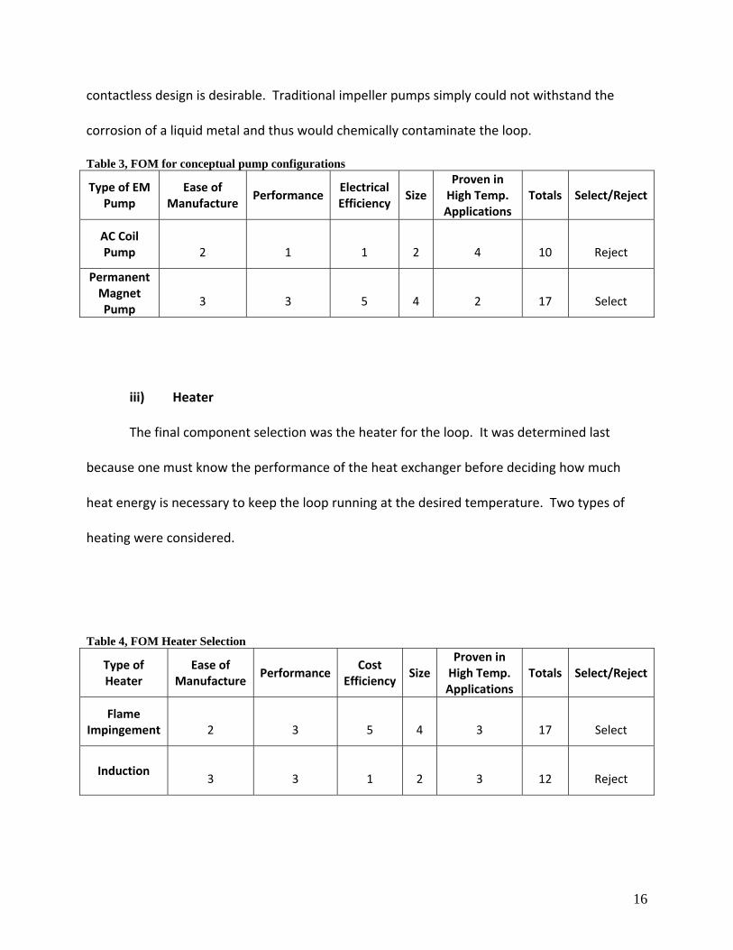
Table 3, FOM for conceptual pump configurations

Type of EM Pump 

Ease of Manufacture 

PerformanceElectrical Efficiency 

SizeProven in High Temp. Applications 

Totals  Select/Reject

AC Coil Pump 

 2 

 1 

 1 

 2 

 4 

 10 

 Reject 

Permanent Magnet Pump 

 3 

 3 

 5 

 4 

 2 

 17 

 Select 

 

 

iii) Heater 

  The final component selection was the heater for the loop.  It was determined last 

because one must know the performance of the heat exchanger before deciding how much 

heat energy is necessary to keep the loop running at the desired temperature.  Two types of 

heating were considered. 

 

 

Table 4, FOM Heater Selection

Type of Heater 

Ease of Manufacture 

PerformanceCost 

EfficiencySize

Proven in High Temp. Applications 

Totals  Select/Reject

Flame Impingement 

 2 

 3 

 5 

 4 

 3 

 17 

 Select 

Induction  3 

 3 

 1 

 2 

 3 

 12 

 Reject 

 

17

  Induction heaters are commercially available in a variety of sizes and power outputs.  

They are typically used in industrial applications where heating metals within non conducting 

pipes is necessary.  These are typically very expensive both in terms of electrical 

energy($11k/year for 11.9kW) and purchase cost($26k) to keep the liquid metal loop at 900 

degrees C.  While a flame impingement heater (natural gas burners) would be a little more 

difficult to set up, maintain, and reject exhaust gasses, natural gas is much cheaper.  11.9kW 

are necessary to maintain 900 C which can be achieved with one natural gas burner (14kW), 

costing $5k/year to run.  No further design was done on heating.    

III.  Preliminary Design 

a) High Temperature Components 

  Now that each design has been considered on the surface, more in depth calculations 

were done to determine which combination of components best suited high temperature 

experimental loop.  Models of the concentric tube heat exchanger, an AC coil type 

electromagnetic pump, and a permanent magnet pump were developed to gauge more 

precisely their performance. 

i) Heat Exchanger Configuration Selection 

   Each configuration was analyzed by hand calculation to formulate a quantifiable 

overview of what performance advantages and disadvantages existed.  The goal is a high ΔT 

and a low overall pressure drop.   The ΔT needed for each exchanger is fixed at a level of 

(250oC) which would enable the study of precipitation and dissolution of solutes in the liquid 

metal.  We also have a known flow rate, 1.2kg/s, to ensure that the test section of fixed 

diameter has a design flow velocity of 0.2m/s, similar to [3].  For a simple  concentric tube 

18

counterflow arrangement, it was determined that an exchanger of 3m in length, with a 1.5in 

OD inner tube and 2.5in ID outer tube could produce this 250oC ΔT.   

  The head loss for the inner tube and the annulus (hydraulic diameter) due to friction for 

a pipe can be calculated as: 

 

 

(1)

where f is the friction factor, which is calculated from the surface roughness, L is the pipe 

length, D is the hydraulic diameter,  is the mass flow rate,   is the fluid density (~9660 

kg/m^3 for 600 oC lead lithium) and g is gravity.  Reaction bonded silicon carbide was assumed 

to have a surface roughness of 110.8nm [10].  Through the use of a common Moody chart and 

the inner and outer tube diameters a friction factors of .015 for the tube side and .0175 for the 

annulus side of the exchanger were obtained.  Using these assumptions, and noting that the 

pressure drop for an internal flow is simply: 

    (2)

  The pressure drop for this counterflow heat exchanger configuration was thus 

determined to be .103psi.   

  For a shell and tube design using commercially available 14mm OD Hexoloy tubing, the 

equation for pressure drop for tube bundles in cross flow becomes: 

 

 (3)

19

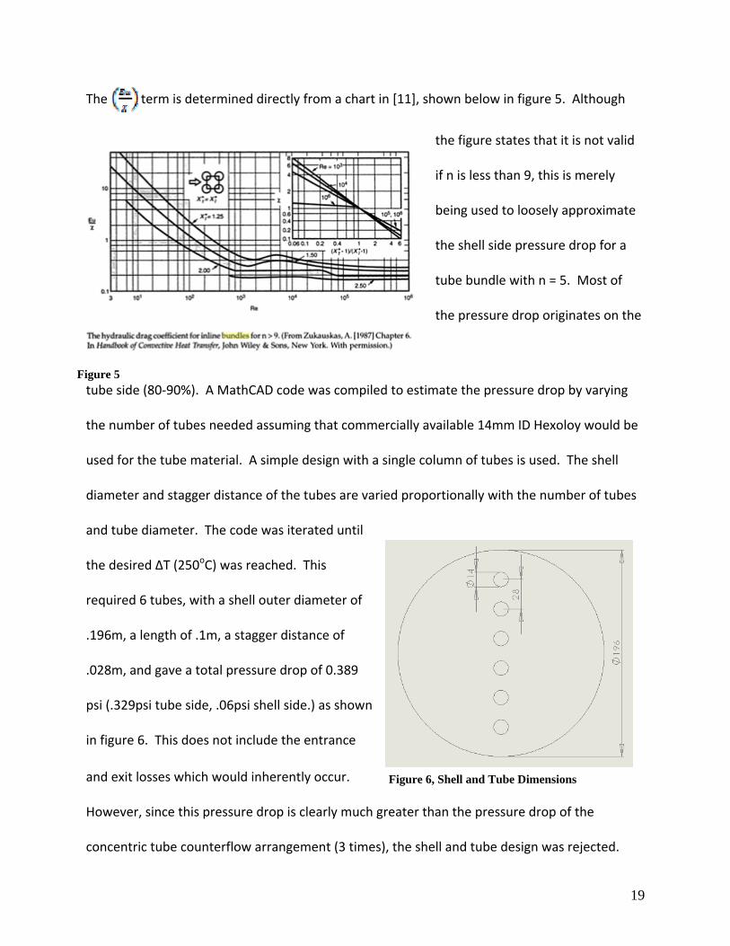
The   term is determined directly from a chart in [11], shown below in figure 5.  Although 

the figure states that it is not valid 

if n is less than 9, this is merely 

being used to loosely approximate 

the shell side pressure drop for a 

tube bundle with n = 5.  Most of 

the pressure drop originates on the 

tube side (80‐90%).  A MathCAD code was compiled to estimate the pressure drop by varying 

the number of tubes needed assuming that commercially available 14mm ID Hexoloy would be  

used for the tube material.  A simple design with a single column of tubes is used.  The shell 

diameter and stagger distance of the tubes are varied proportionally with the number of tubes 

and tube diameter.  The code was iterated until 

the desired ΔT (250oC) was reached.  This 

required 6 tubes, with a shell outer diameter of 

.196m, a length of .1m, a stagger distance of 

.028m, and gave a total pressure drop of 0.389 

psi (.329psi tube side, .06psi shell side.) as shown 

in figure 6.  This does not include the entrance 

and exit losses which would inherently occur.  

However, since this pressure drop is clearly much greater than the pressure drop of the 

concentric tube counterflow arrangement (3 times), the shell and tube design was rejected.  

Figure 5

Figure 6, Shell and Tube Dimensions 

Figure 5

20

Also, this decision reinforced by the difficulty of building a compact heat exchanger for a high 

temperature application along with the increased risk of leakage from the many bonds required 

to seal it as shown in table 2. 

ii)  Concentric Tube Heat Exchanger Model and Heater Application 

  A computer model of a high temperature counterflow heat exchanger was created in 

order to understand how the real exchanger would perform, given the properties of Pb‐17Li 

and silicon carbide.  Fluid properties vary as a function of fluid temperature and therefore have 

an effect on the transfer of heat radially and axially across the exchanger. 

  This would prove the feasibility of this design.  It is a simple 1‐D code (radial for 

concentric pipes).   The pump’s purpose is to reheat the cold fluid from the dump tank of a high 

temperature loop before it gets to a heater, and lastly the test section.    This would save 

energy used by a heater and decrease the number of heaters necessary.   For the best efficiency 

and performance given the flow conditions, it was decided the HX be constructed in a counter‐

flow arrangement with the hot fluid entering the inner tube.   The study here is to determine a 

suitable length of the exchanger, and how much insulation will be necessary as to maximize the 

heat transfer rate.  Also, design possibilities including a rough layout of an experimental loop 

will be discussed, based on the code results. 

1. Abstract 

  A simple approach was taken to write this computer model.  MATLAB 7.0 was used.  

Heat is transferred due to convection between the moving fluids and air as well as conduction 

between the fluids through the walls of the tubing as well as conduction in the fluid itself, due 

to the high conductivity of liquid metals.  The overall result of running the code is that after the 

21

user defines simply the mass flow rate in kg/s for each fluid, the program outputs 2 plots.   

These plots aided in the selection of an appropriate length for the heat exchanger.  A 10m 

counterflow heat exchanger resulted with a 1.5” OD inner hot fluid pipe and a concentric 2” OD 

outer cold fluid annulus.  The hot fluid enters at 900 degrees C and exits at 267 degrees C, while 

the cold fluid enters around 250 degrees C and is reheated to 846 degrees C.  A conceptual 

design for the loop was also generated based on the findings of this report.   

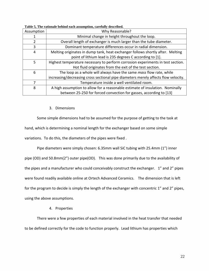
2. Assumptions 

Some simple assumptions were necessary: 

1.  Negligible kinetic and potential energy changes 

2.  Fully developed conditions for Li‐17Pb 

3. Heat loss is in the radial direction only 

4. Entering cold fluid temperature is 250 degrees C 

5. Entering hot fluid temperature is 900 degrees C 

6. Mass flow rate in both pipes is identical 

7. Ambient air is at 25 degrees C 

8. Convection heat transfer coefficient for air is 40 [W/(m*K)] 

Here, a brief explanation for each assumption is provided.  

 

 

 

 

22

Table 5, The rationale behind each assumption, carefully described. Assumption  Why Reasonable? 

1  Minimal change in height throughout the loop. 2  Overall length of exchanger is much larger than the tube diameter. 3  Dominant temperature differences occur in radial dimension. 4  Melting originates in dump tank, heat exchanger follows shortly after.  Melting 

point of lithium lead is 235 degrees C according to [1]. 5  Highest temperature necessary to perform corrosion experiments in test section.  

Hot fluid originates from the exit of the test section.  6  The loop as a whole will always have the same mass flow rate, while 

increasing/decreasing cross sectional pipe diameters merely affects flow velocity. 7  Temperature inside a well ventilated room. 8  A high assumption to allow for a reasonable estimate of insulation.  Nominally 

between 25‐250 for forced convection for gasses, according to [13]  

3. Dimensions 

  Some simple dimensions had to be assumed for the purpose of getting to the task at 

hand, which is determining a nominal length for the exchanger based on some simple 

variations.  To do this, the diameters of the pipes were fixed . 

Pipe diameters were simply chosen: 6.35mm wall SiC tubing with 25.4mm (1”) inner 

pipe (OD) and 50.8mm(2”) outer pipe(OD).   This was done primarily due to the availability of 

the pipes and a manufacturer who could conceivably construct the exchanger.   1” and 2” pipes 

were found readily available online at Ortech Advanced Ceramics.    The dimension that is left 

for the program to decide is simply the length of the exchanger with concentric 1” and 2” pipes, 

using the above assumptions. 

4. Properties 

  There were a few properties of each material involved in the heat transfer that needed 

to be defined correctly for the code to function properly.  Lead lithium has properties which 

23

vary depending on temperature, and this was taken into account.  For the thermal conductivity, 

k, values were taken from previous UCSD ARIES team research [12] in the form: 

        (4)

Density, ρ, and specific heat,  , must also be considered a function of temperature where: 

       (5)

 

          (6)

5. Theory 

  Now the variables in the code must be solved for.  First and foremost the convection 

between the hot and cold fluids, the dominant driver for heat transfer, will be evaluated.  We 

will assume here that there is no losses to the surroundings for simplicity, but will then account 

for these losses later.   Reynolds number in both the inner and outer pipes must be calculated.  

For the hot fluid in the tube, with a few manipulations using hydraulic diameters: 

          (7)

where U is the flow velocity in m/s,   is the mass flow rate of the hot fluid in kg/s,   

is simply the difference in average inner and outer pipe diameters in meters, with   the 

viscosity of the fluid in kg/(m*s).  It is important to note that a Re larger that 4000 would be 

turbulent and that for lead lithium, it is rare even in extremely small flow rates for the flow to 

be laminar due to the density of the fluid.  For example with a flow rate of 0.1kg/s, the Re is 

around 9000.  The Prandtl number Pr must also be calculated.   This number is affected by 

specific heat, viscosity and thermal conductivity of a moving fluid. 

24

          (8)   

  

The Nusselt number must be calculated.  There are many different methods of 

calculating this, however only one best fit the current setup of the heat exchanger.  For initial 

calculations the Dittus‐Boelter equation was used as follows with   for cooling, and   

for heating:   

          (9)

  It was later thought that the conductive nature and low Prandtl numbers of lead lithium 

render the Dittus‐Boelter equation assumptions incorrect.  Thus, a new correlation first 

implemented by Lyon [14] and used in the final revision of the MATLAB code.  It is specific to 

turbulent, liquid metal coolants flowing in circular tubes assuming a constant heat flux along 

the tube wall:  

          (10)

where Pe is the Peclet number, which is calculated simply by multiplying the Reynolds number 

by the Prandtl number.   

Next the convection heat transfer coefficient is calculated with the following simple relation: 

              (11)

  For the cold fluid, the same values are needed however, the   is calculated differently 

because of the pipe geometry.  The hot fluid is in an annulus and the cold fluid is simply in a 

pipe: 

              (12)

25

where    is the mass flow rate of the cold fluid.  From here the Nusselt number for cold fluid 

must also be calculated using equation 6, but with n = 0.4 for heating the incoming cold fluid.  

Equations 5 and 7 are identical for the cold fluid case.  After running through these equations 

for both cases, calculating the convection heat transfer coefficient for both hot and cold fluids, 

the final step in terms of convection  can take place: 

                 (13)

  U is the overall heat transfer coefficient for the counter flow heat exchanger.  It will 

allow us to calculate a heat transfer rate and thus the length, L in meters, of the heat exchanger 

necessary to achieve this heat transfer rate, Q in watts.  Keeping in mind that assumption 6 in 

table 1 tells us that the mass flow rates for the hot and cold fluids must be equal: 

                      (14)

Where   is known from assumption 5 and where the hot fluid temperature flow out,  , is 

iterated in the MATLAB code between 539 and 310 degrees C.  This makes Q into a column 

vector, with increasing Q as the hot fluid temperature out decreases.  With Q known, we can 

now calculate the cold fluid temperature out, giving us a log mean temperature difference, and 

thus the necessary length of the heat exchanger.   

                      (15)

Where   is the specific heat of the cold fluid in degrees, based on temperature from equation 

(8). 

26

                           (16)

Here the cold temperature in,  , as well as   is known from assumptions 4 and 5 

respectively.   

                      (17)

 

 

 (18)

 

  The length of the heat exchanger is now known which produces the heat transfer rate 

Q, assuming that there are not losses.  Now we must rid ourselves of the no losses assumption.  

To do this, we’ll use this initial length we’ve just calculated to estimate a  .   We need to 

know how long the exchanger is to estimate how much heat is being lost to the surroundings 

through conduction between the SiC pipes and the insulation to the surroundings.  The length 

calculated without losses in (13) will then be increased to accommodate for this leak of heat to 

the surroundings. 

  The heat has 3 modes of escaping our ideal model into the surroundings.  They have to 

do with the thermal resistance of the SiC inner/outer pipes , the layer of insulation, and the 

convection to the surrounding air.   They can be characterized as follows: 

 

 (19)

 

27

         (20)

 

             (21)

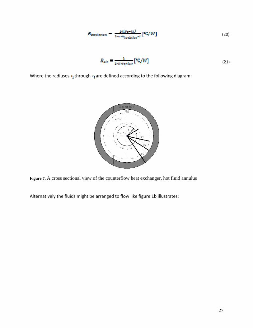
Where the radiuses  through  are defined according to the following diagram: 

 

Figure 7, A cross sectional view of the counterflow heat exchanger, hot fluid annulus  

Alternatively the fluids might be arranged to flow like figure 1b illustrates: 

 

28

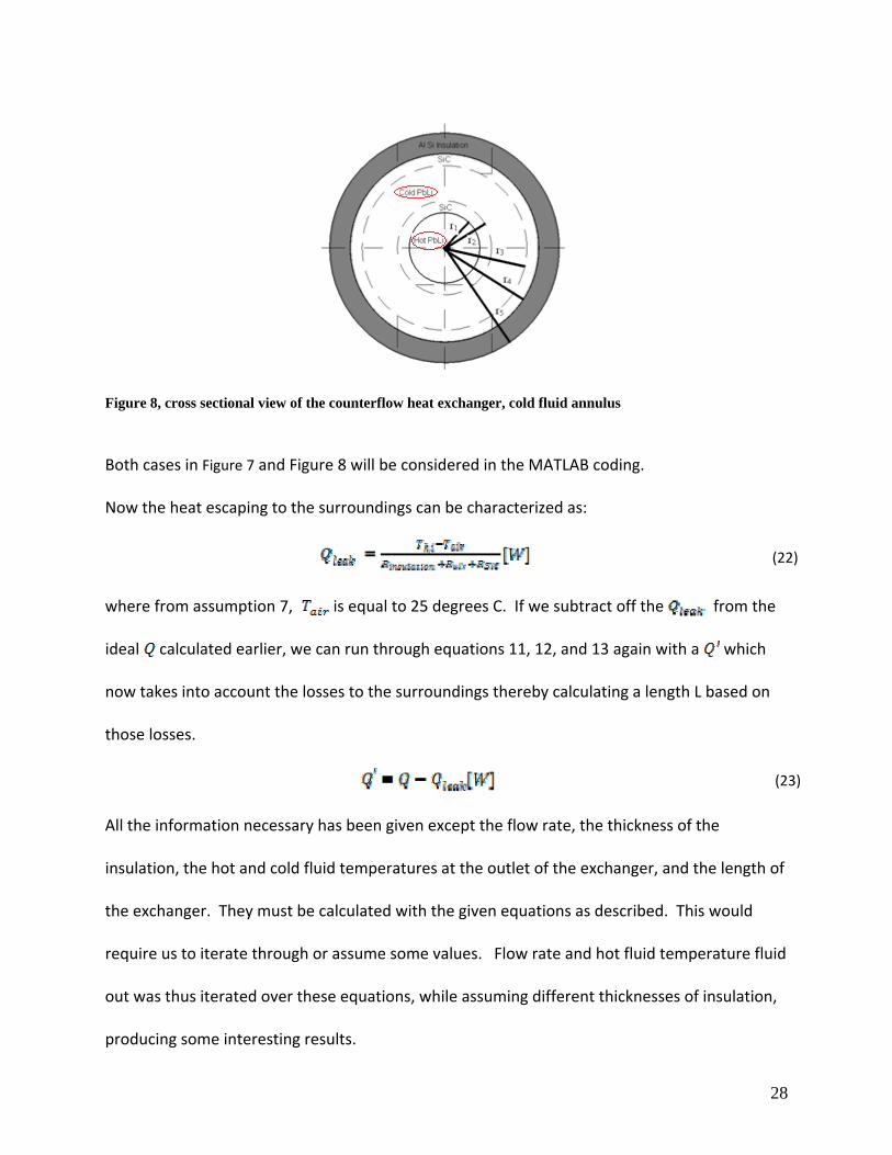
Figure 8, cross sectional view of the counterflow heat exchanger, cold fluid annulus  

Both cases in Figure 7 and Figure 8 will be considered in the MATLAB coding. 

Now the heat escaping to the surroundings can be characterized as: 

         (22)

where from assumption 7,    is equal to 25 degrees C.  If we subtract off the   from the 

ideal   calculated earlier, we can run through equations 11, 12, and 13 again with a   which 

now takes into account the losses to the surroundings thereby calculating a length L based on 

those losses.   

         (23)

All the information necessary has been given except the flow rate, the thickness of the 

insulation, the hot and cold fluid temperatures at the outlet of the exchanger, and the length of 

the exchanger.  They must be calculated with the given equations as described.  This would 

require us to iterate through or assume some values.   Flow rate and hot fluid temperature fluid 

out was thus iterated over these equations, while assuming different thicknesses of insulation, 

producing some interesting results. 

29

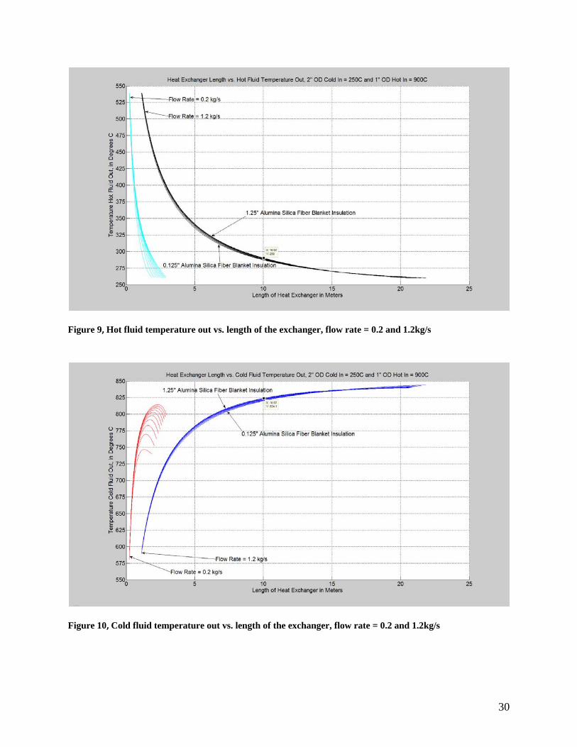
6. Results 

  Since the loop at FZK in Germany tested 8mm specimens at 0.22m/s flow velocity in a 

16mm test section producing a mass flow rate of about 1.2 kg/s , the results here will focus on 

that flow rate, while other flow rates were tested for heat transfer ability.  The code in MATLAB 

produces three graphs as previously described in the abstract.  These graphs were produced for 

different flow conditions with different thicknesses of an Alumina Silica insulation.  It appears 

that from the following results, a 10 meter long heat exchanger and a layer of 1.25” AlSi 

insulation would be sufficient to reheat the cold fluid to 824 degrees C for a 1.2kg/s flow rate.  

The slower flow rate, 0.2 kg/s, the heat exchanger could reheat the cold fluid to about 817 

degrees in only 2 meters, as shown in figure 3.   

Now, with a flow rate of 0.2 and 1.2 kg/s, the following graphs were produced based on the 

solutions of the iterated values discussed previously, and a flow arrangement analogous with 

figure 1a. 

30

Figure 9, Hot fluid temperature out vs. length of the exchanger, flow rate = 0.2 and 1.2kg/s  

Figure 10, Cold fluid temperature out vs. length of the exchanger, flow rate = 0.2 and 1.2kg/s  

31

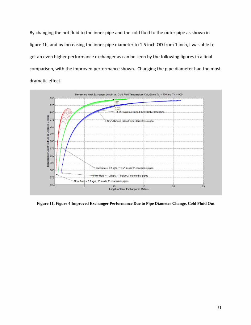
By changing the hot fluid to the inner pipe and the cold fluid to the outer pipe as shown in 

figure 1b, and by increasing the inner pipe diameter to 1.5 inch OD from 1 inch, I was able to 

get an even higher performance exchanger as can be seen by the following figures in a final 

comparison, with the improved performance shown.  Changing the pipe diameter had the most 

dramatic effect. 

Figure 11, Figure 4 Improved Exchanger Performance Due to Pipe Diameter Change, Cold Fluid Out

32

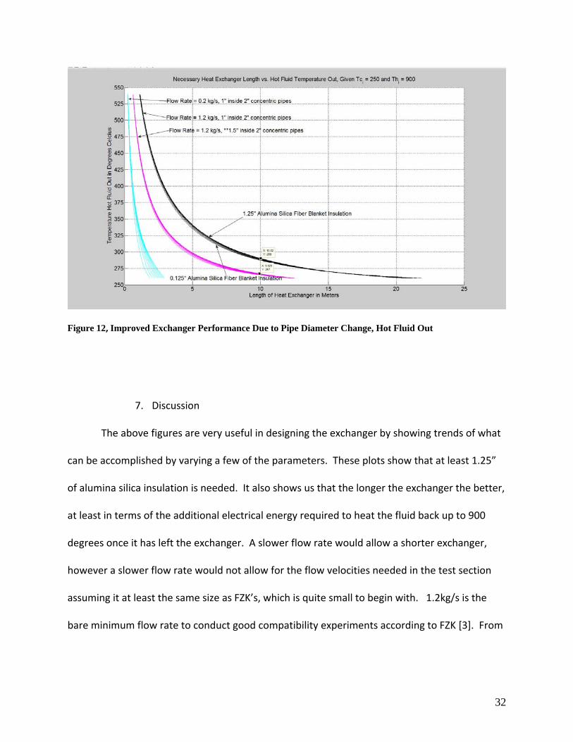
Figure 12, Improved Exchanger Performance Due to Pipe Diameter Change, Hot Fluid Out

7. Discussion 

The above figures are very useful in designing the exchanger by showing trends of what 

can be accomplished by varying a few of the parameters.  These plots show that at least 1.25” 

of alumina silica insulation is needed.  It also shows us that the longer the exchanger the better, 

at least in terms of the additional electrical energy required to heat the fluid back up to 900 

degrees once it has left the exchanger.  A slower flow rate would allow a shorter exchanger, 

however a slower flow rate would not allow for the flow velocities needed in the test section 

assuming it at least the same size as FZK’s, which is quite small to begin with.   1.2kg/s is the 

bare minimum flow rate to conduct good compatibility experiments according to FZK [3].  From 

33

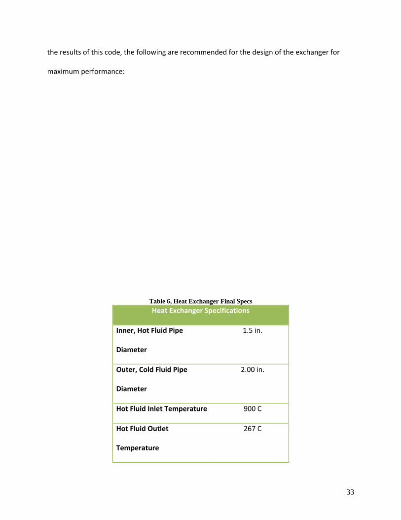
the results of this code, the following are recommended for the design of the exchanger for 

maximum performance: 

 

 

 

 

 

 

 

 

 

 

 

Table 6, Heat Exchanger Final Specs Heat Exchanger Specifications 

Inner, Hot Fluid Pipe 

Diameter 

1.5 in. 

Outer, Cold Fluid Pipe 

Diameter 

2.00 in. 

Hot Fluid Inlet Temperature  900 C 

Hot Fluid Outlet 

Temperature 

267 C 

34

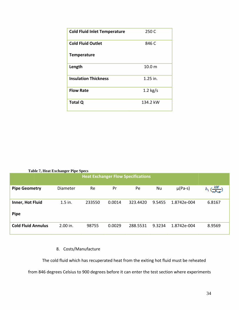
Cold Fluid Inlet Temperature  250 C 

Cold Fluid Outlet 

Temperature 

846 C 

Length  10.0 m 

Insulation Thickness  1.25 in. 

Flow Rate  1.2 kg/s 

Total Q  134.2 kW 

 

 

 

 

 

Table 7, Heat Exchanger Pipe Specs   Heat Exchanger Flow Specifications   

Pipe Geometry  Diameter  Re  Pr  Pe  Nu  μ(Pa‐s)     

Inner, Hot Fluid 

Pipe  

1.5 in.  233550  0.0014  323.4420  9.5455 1.8742e‐004  6.8167 

Cold Fluid Annulus   2.00 in.  98755  0.0029  288.5531  9.3234 1.8742e‐004  8.9569 

 

8. Costs/Manufacture 

  The cold fluid which has recuperated heat from the exiting hot fluid must be reheated 

from 846 degrees Celsius to 900 degrees before it can enter the test section where experiments 

35

will be conducted.  Using equation 10 one can calculate that the heat necessary to get the fluid 

from 846 to 900 degrees C is 11.9kW.  This can be accomplished with a variety of RF induction 

heaters, which can selectively heat the lead lithium but not the silicon carbide piping.  The loop 

will take time to “start up”, in other words, get up to temperature.  The time needed will 

depend greatly on the amount of maximum heat the induction heater can provide.  

Continuously, however, the induction heater will only need 11.9kW after the start up time.  To 

ensure a fast start up time, I would recommend the 60kW induction heater from the Superior 

Induction Company as a reliable source of energy.  The heater itself runs between $26 k and 

$27k.  Typical electrical costs in San Diego, CA are 10 cents per kWh.  If the heater ran for a year 

continuously, this would amount to 104.2MWh, or cost approximately $10,424 per year to run, 

plus the start up time cost which the heater would typically run hotter, and plus the costs of lab 

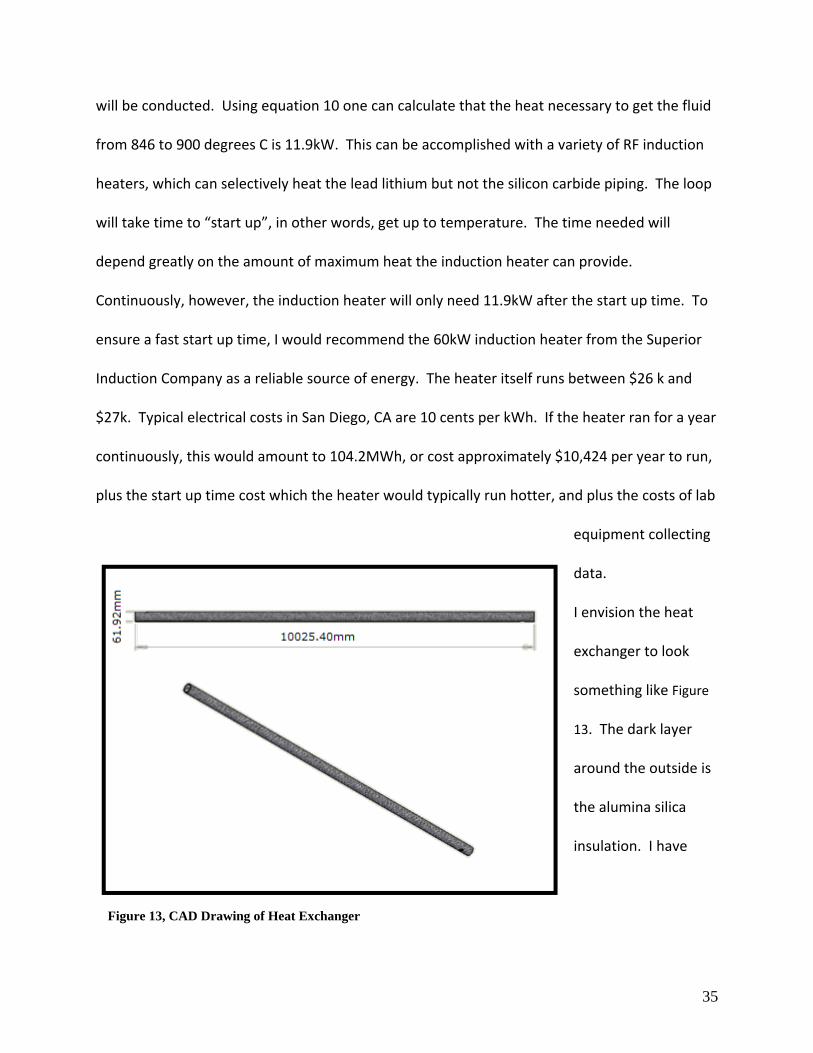
equipment collecting 

data. 

I envision the heat 

exchanger to look 

something like Figure 

13.  The dark layer 

around the outside is 

the alumina silica 

insulation.  I have 

Figure 13, CAD Drawing of Heat Exchanger

36

spoken with Zircar Ceramics who can provide us with the “ASH” material. 

I have spoken with an engineer from graphitestore.com who believes that so long as the 

curing process is followed closely (requiring baking),  that Ceramabond 503 compound would 

withstand our high temperatures and be able to bond SiC tubing.  Alternatively, Ortech 

ceramics says they are able to fire SiC tubes together, and that while the bond may not be as 

strong as “normal” it would hold temperature.  Ceramabond 503 costs $92.81 a pint.   The 

engineer at graphitestore.com also recommended that for an easier curing time, but not so 

quite ideal bond, an alumina nitride adhesive, Ceramabond 865, would also work and survive 

the same temperature.  It is a little more expensive at $124.82 a pint.  I recommend ordering 

the concentric SiC tubes, bonding caps on the ends and drilling holes in the outside of the outer 

tube for inlet and exit of the cold fluid. 

  The SiC heat exchanger is feasible after contacting some of the vendors and talking with 

them about these different methods of bonding and adhering.  The cost of electricity was a 

significant factor in choosing components for this project.  One last fouling possibility is the 

“shorting out” of the heat exchanger through the SiC down the length of the tube axially.  This 

could pose a  serious problem.   I have roughly calculated that with equation 19, where A is the 

cross sectional area and x is along the length of the heat exchanger in meters.   

     [W]          (24)

With a temperature difference of 626 degrees C, the heat transfer is 12.26W.  This is a trivial 

amount of heat lost compared to the 134kW of heat moving radially, further solidifying my 

previous assumption.  This assumption holds in [14] for Peclet numbers greater than 35.  The 

lowest Pe as shown in table 3 is 288. 

37

iii) High Temperature Pumping Components 

  Upon initial conceptual analysis, the AC coil pump design is rejected.  Its electrical 

efficiency was deemed poor in comparison with the permanent magnet pump.  The permanent 

magnet pump has cheap raw materials, is easy to construct, and is much more compact than 

the permanent magnet pump.  It also does not have coils that need to be cooled due to the 

ohmic dissipation of heat.  However, since the FOM in Table 3 is close, and research was done 

on both methods, both are considered here. 

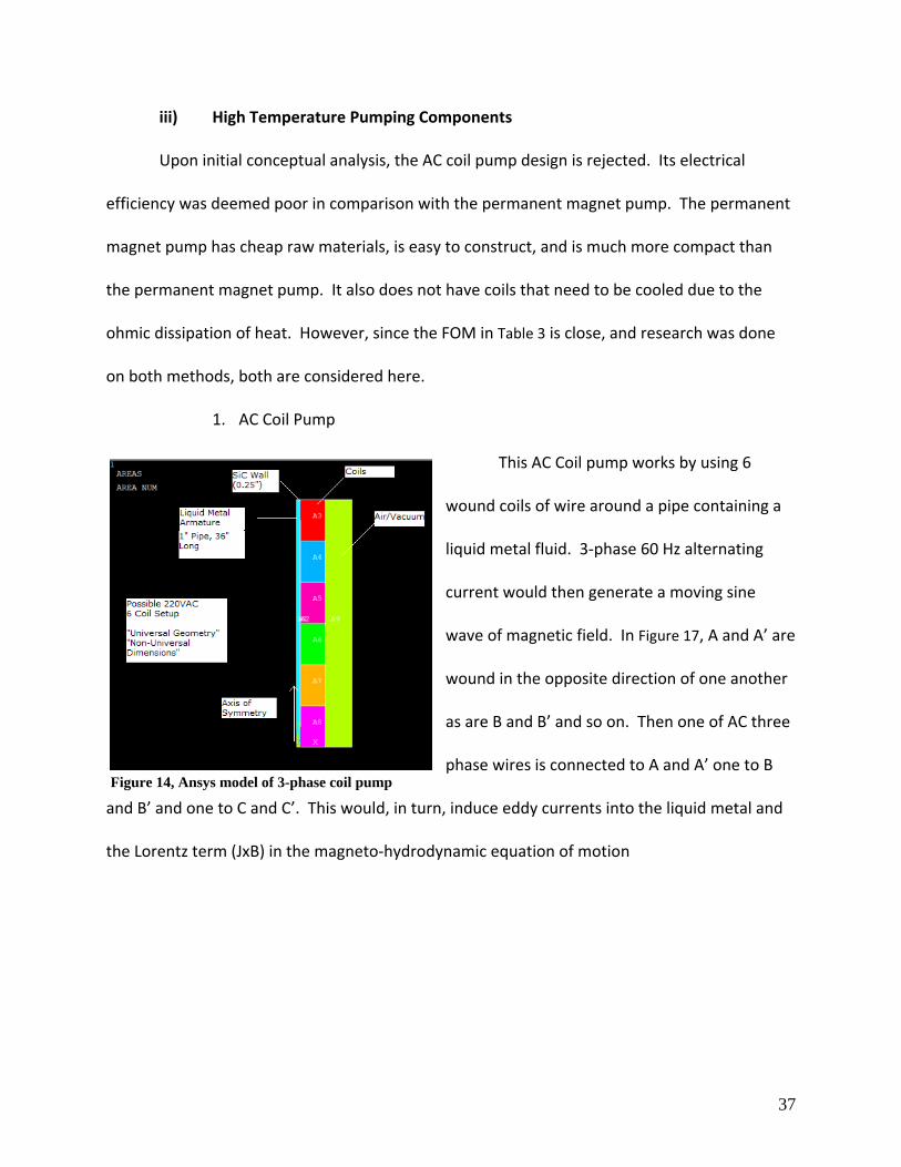
1. AC Coil Pump 

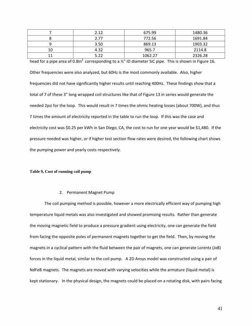
  This AC Coil pump works by using 6 

wound coils of wire around a pipe containing a 

liquid metal fluid.  3‐phase 60 Hz alternating 

current would then generate a moving sine 

wave of magnetic field.  In Figure 17, A and A’ are 

wound in the opposite direction of one another 

as are B and B’ and so on.  Then one of AC three 

phase wires is connected to A and A’ one to B 

and B’ and one to C and C’.  This would, in turn, induce eddy currents into the liquid metal and 

the Lorentz term (JxB) in the magneto‐hydrodynamic equation of motion  

Figure 14, Ansys model of 3-phase coil pump

38

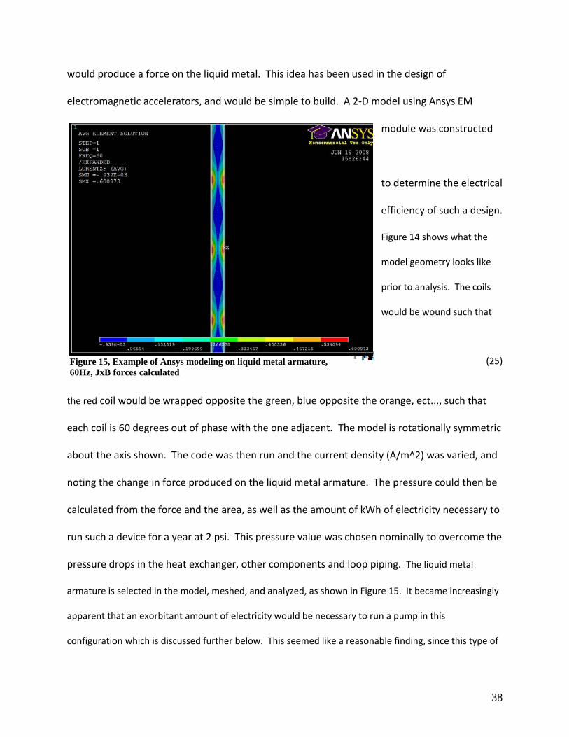
would produce a force on the liquid metal.  This idea has been used in the design of 

electromagnetic accelerators, and would be simple to build.  A 2‐D model using Ansys EM 

module was constructed  

 

to determine the electrical 

efficiency of such a design.  

Figure 14 shows what the 

model geometry looks like 

prior to analysis.  The coils 

would be wound such that 

the red coil would be wrapped opposite the green, blue opposite the orange, ect..., such that 

each coil is 60 degrees out of phase with the one adjacent.  The model is rotationally symmetric 

about the axis shown.  The code was then run and the current density (A/m^2) was varied, and 

noting the change in force produced on the liquid metal armature.  The pressure could then be 

calculated from the force and the area, as well as the amount of kWh of electricity necessary to 

run such a device for a year at 2 psi.  This pressure value was chosen nominally to overcome the 

pressure drops in the heat exchanger, other components and loop piping.  The liquid metal 

armature is selected in the model, meshed, and analyzed, as shown in Figure 15.  It became increasingly 

apparent that an exorbitant amount of electricity would be necessary to run a pump in this 

configuration which is discussed further below.  This seemed like a reasonable finding, since this type of 

 

 

(25)Figure 15, Example of Ansys modeling on liquid metal armature, 60Hz, JxB forces calculated 

39

design is used in solid target accelerators, where large amounts of electricity for short amounts of time 

are necessary.  However, for a long term application where the pump will run for a year or more, the 

high cost and operating conditions (i.e. temperature of coils) become problems.  Iteration with a model 

was necessary to determine the maximum amount of current allowable in the coils before overheating.   

  A Mathcad model was constructed to determine the maximum current density attainable 

considering the ohmic heating losses incurred by wrapped coils.  To improve performance, a cooling 

water jacket of 1in diameter was used around the coils.   

 

Input Parameters    Outputs Parameters  Magnet Wire Diameter  35AWG, 0.08mm Ohmic Heating Loses 96.57 W

Voltage on Coil  220V  Coil Current 2.634 ALength of 6 coils  .25ft  Coil Surface Temp 36.15 oC

ID of Coil Wrap  .5in  Chilled Water Flow Rate  3.435   

Chilled Water Pipe OD  1.00in  Current Density 864.111kA/m2

Maximum Wire Temperature 

200C (high temp insulation) 

Total Number of 6 phase coils  to Meet 2psi Demand 

7 

Table 8, Mathcad model output for coil pump cooling/current requirements

40

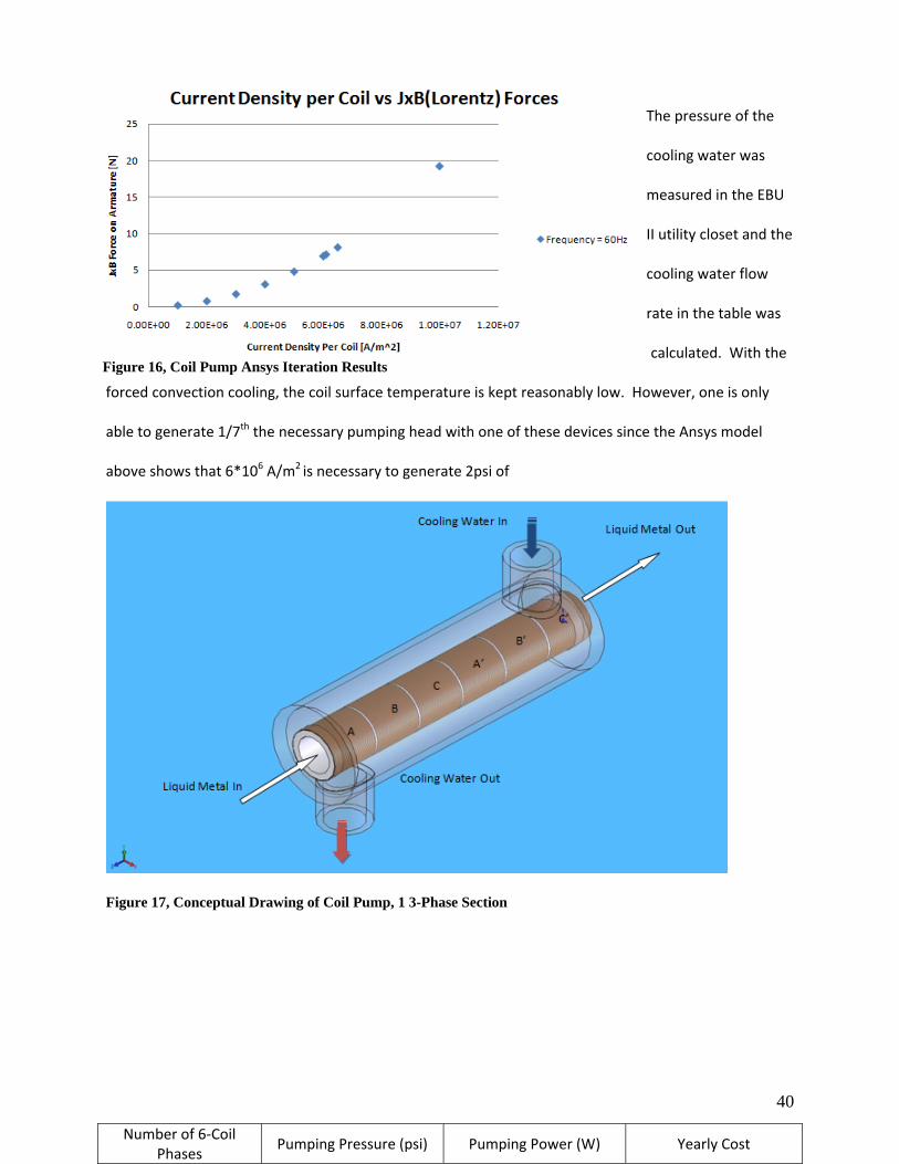
The pressure of the 

cooling water was 

measured in the EBU 

II utility closet and the 

cooling water flow 

rate in the table was 

calculated.  With the  

forced convection cooling, the coil surface temperature is kept reasonably low.  However, one is only 

able to generate 1/7th the necessary pumping head with one of these devices since the Ansys model 

above shows that 6*106 A/m2 is necessary to generate 2psi of  

Figure 17, Conceptual Drawing of Coil Pump, 1 3-Phase Section

Number of 6‐Coil Phases 

Pumping Pressure (psi)  Pumping Power (W)  Yearly Cost 

Figure 16, Coil Pump Ansys Iteration Results

41

head for a pipe area of 0.8in2  corresponding to a ½” ID diameter SiC pipe.  This is shown in Figure 16.   

Other frequencies were also analyzed, but 60Hz is the most commonly available.  Also, higher 

frequencies did not have significantly higher results until reaching 400Hz.  These findings show that a 

total of 7 of these 3” long wrapped coil structures like that of Figure 13 in series would generate the 

needed 2psi for the loop.  This would result in 7 times the ohmic heating losses (about 700W), and thus 

7 times the amount of electricity reported in the table to run the loop.  If this was the case and 

electricity cost was $0.25 per kWh in San Diego, CA, the cost to run for one year would be $1,480.  If the 

pressure needed was higher, or if higher test section flow rates were desired, the following chart shows 

the pumping power and yearly costs respectively. 

 

Table 9, Cost of running coil pump  

   

2. Permanent Magnet Pump 

  The coil pumping method is possible, however a more electrically efficient way of pumping high 

temperature liquid metals was also investigated and showed promising results.  Rather than generate 

the moving magnetic field to produce a pressure gradient using electricity, one can generate the field 

from facing the opposite poles of permanent magnets together to get the field.  Then, by moving the 

magnets in a cyclical pattern with the fluid between the pair of magnets, one can generate Lorentz (JxB) 

forces in the liquid metal, similar to the coil pump.   A 2D Ansys model was constructed using a pair of 

NdFeB magnets.  The magnets are moved with varying velocities while the armature (liquid metal) is 

kept stationary.   In the physical design, the magnets could be placed on a rotating disk, with pairs facing 

7  2.12  675.99  1480.36 8  2.77  772.56  1691.84 9  3.50  869.13  1903.32 10  4.32  965.7  2114.8 11  5.22  1062.27  2326.28 

42

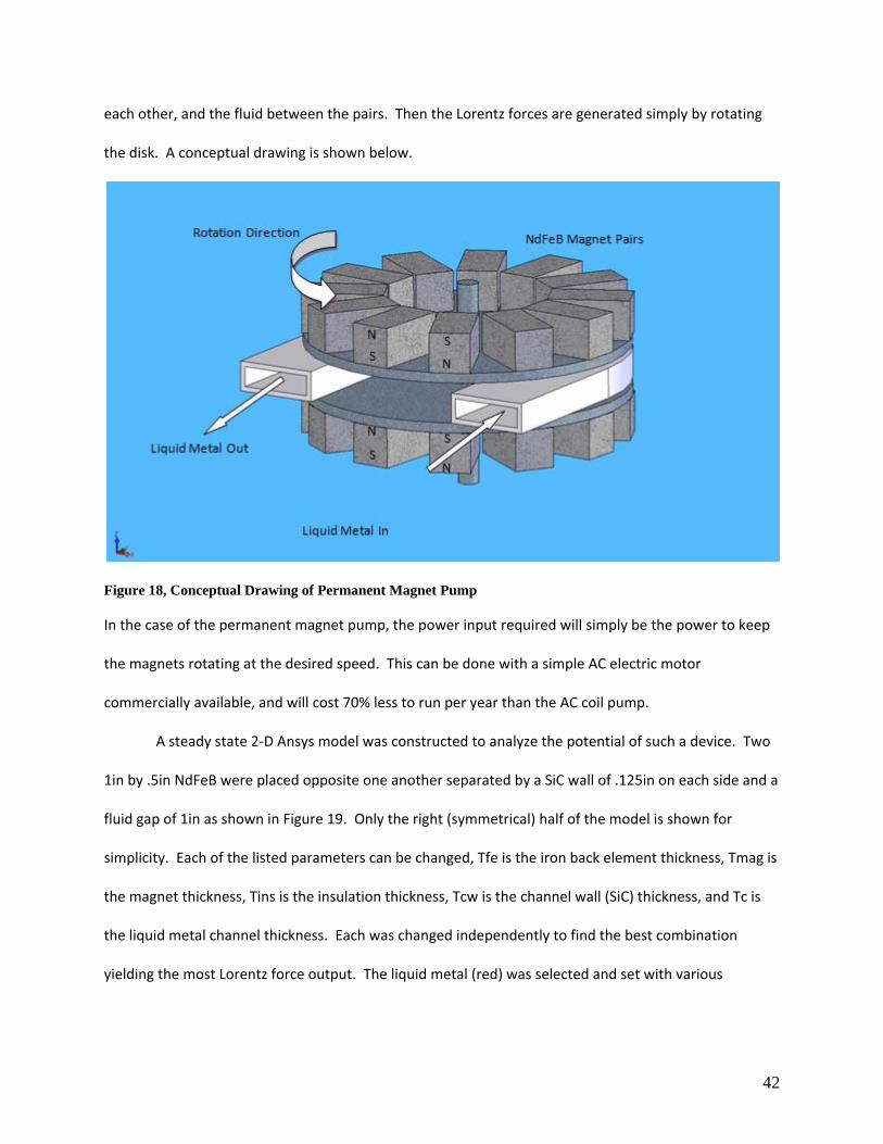
each other, and the fluid between the pairs.  Then the Lorentz forces are generated simply by rotating 

the disk.  A conceptual drawing is shown below.     

   Figure 18, Conceptual Drawing of Permanent Magnet Pump

In the case of the permanent magnet pump, the power input required will simply be the power to keep 

the magnets rotating at the desired speed.  This can be done with a simple AC electric motor 

commercially available, and will cost 70% less to run per year than the AC coil pump.   

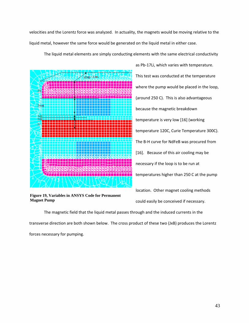
  A steady state 2‐D Ansys model was constructed to analyze the potential of such a device.  Two 

1in by .5in NdFeB were placed opposite one another separated by a SiC wall of .125in on each side and a 

fluid gap of 1in as shown in Figure 19. Only the right (symmetrical) half of the model is shown for 

simplicity.  Each of the listed parameters can be changed, Tfe is the iron back element thickness, Tmag is 

the magnet thickness, Tins is the insulation thickness, Tcw is the channel wall (SiC) thickness, and Tc is 

the liquid metal channel thickness.  Each was changed independently to find the best combination 

yielding the most Lorentz force output.  The liquid metal (red) was selected and set with various 

43

velocities and the Lorentz force was analyzed.  In actuality, the magnets would be moving relative to the 

liquid metal, however the same force would be generated on the liquid metal in either case.   

The liquid metal elements are simply conducting elements with the same electrical conductivity 

as Pb‐17Li, which varies with temperature.   

This test was conducted at the temperature 

where the pump would be placed in the loop, 

(around 250 C).  This is also advantageous 

because the magnetic breakdown 

temperature is very low [16] (working 

temperature 120C, Curie Temperature 300C).  

The B‐H curve for NdFeB was procured from 

[16].   Because of this air cooling may be 

necessary if the loop is to be run at 

temperatures higher than 250 C at the pump 

location.  Other magnet cooling methods 

could easily be conceived if necessary.  

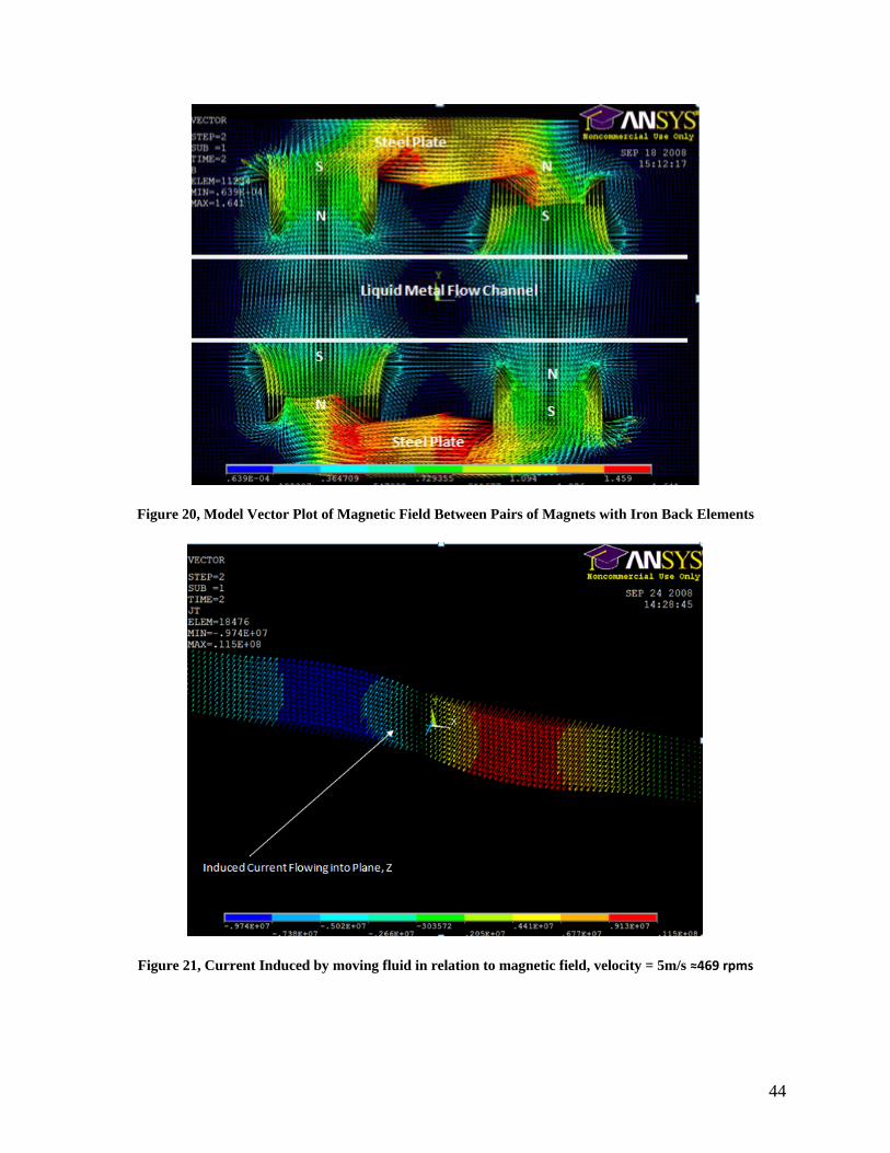
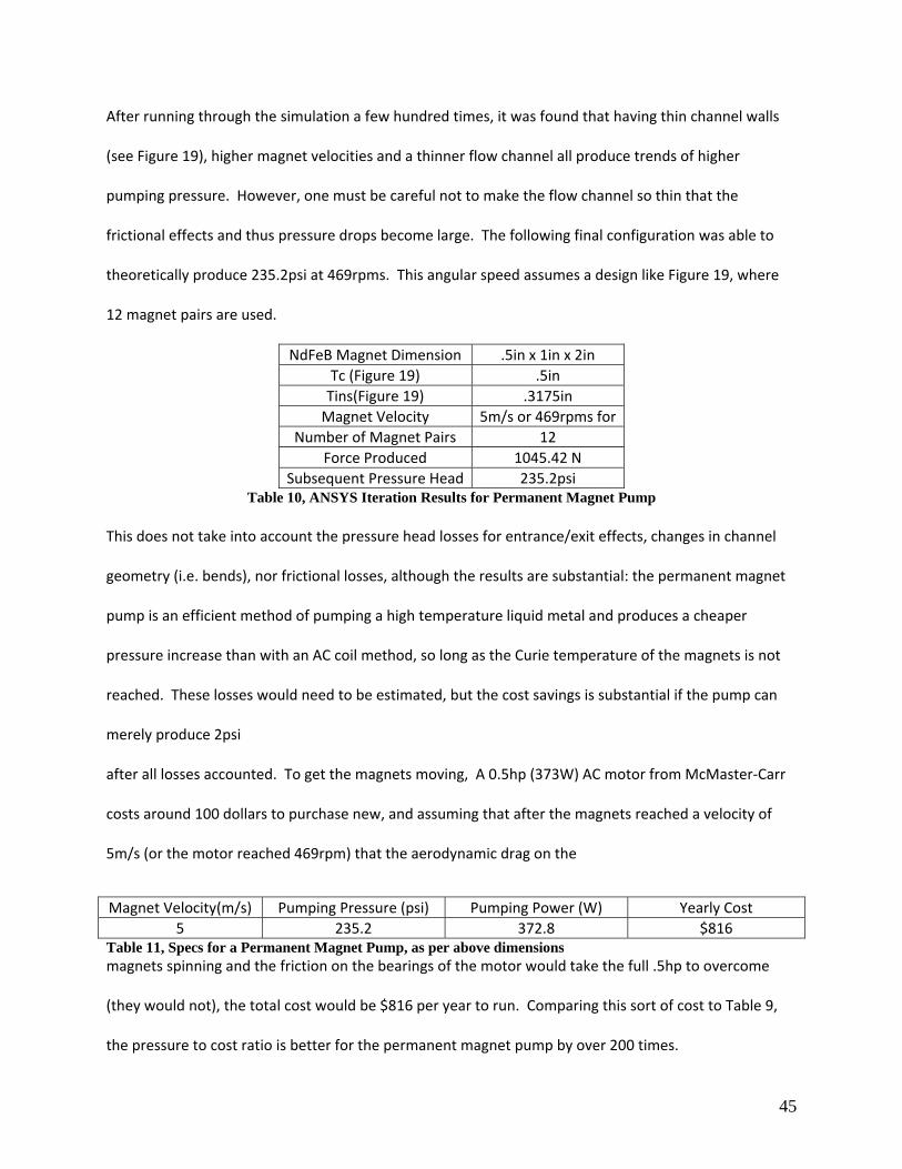
  The magnetic field that the liquid metal passes through and the induced currents in the 

transverse direction are both shown below.  The cross product of these two (JxB) produces the Lorentz 

forces necessary for pumping. 

Figure 19, Variables in ANSYS Code for Permanent Magnet Pump

44

Figure 20, Model Vector Plot of Magnetic Field Between Pairs of Magnets with Iron Back Elements

 

Figure 21, Current Induced by moving fluid in relation to magnetic field, velocity = 5m/s ≈469 rpms  

 

45

After running through the simulation a few hundred times, it was found that having thin channel walls 

(see Figure 19), higher magnet velocities and a thinner flow channel all produce trends of higher 

pumping pressure.  However, one must be careful not to make the flow channel so thin that the 

frictional effects and thus pressure drops become large.  The following final configuration was able to 

theoretically produce 235.2psi at 469rpms.  This angular speed assumes a design like Figure 19, where 

12 magnet pairs are used.   

NdFeB Magnet Dimension  .5in x 1in x 2in Tc (Figure 19)  .5in Tins(Figure 19)  .3175in Magnet Velocity  5m/s or 469rpms for

Number of Magnet Pairs  12 Force Produced  1045.42 N 

Subsequent Pressure Head 235.2psi Table 10, ANSYS Iteration Results for Permanent Magnet Pump

This does not take into account the pressure head losses for entrance/exit effects, changes in channel 

geometry (i.e. bends), nor frictional losses, although the results are substantial: the permanent magnet 

pump is an efficient method of pumping a high temperature liquid metal and produces a cheaper 

pressure increase than with an AC coil method, so long as the Curie temperature of the magnets is not 

reached.  These losses would need to be estimated, but the cost savings is substantial if the pump can 

merely produce 2psi  

after all losses accounted.  To get the magnets moving,  A 0.5hp (373W) AC motor from McMaster‐Carr 

costs around 100 dollars to purchase new, and assuming that after the magnets reached a velocity of 

5m/s (or the motor reached 469rpm) that the aerodynamic drag on the 

Table 11, Specs for a Permanent Magnet Pump, as per above dimensions magnets spinning and the friction on the bearings of the motor would take the full .5hp to overcome 

(they would not), the total cost would be $816 per year to run.  Comparing this sort of cost to Table 9, 

the pressure to cost ratio is better for the permanent magnet pump by over 200 times. 

Magnet Velocity(m/s)  Pumping Pressure (psi)  Pumping Power (W)  Yearly Cost 5  235.2  372.8  $816 

46

IV. Conclusions 

The loop components have now all been successfully analyzed and decided upon.   A loop with 

a flame impingement heater, concentric tube heat exchanger, and permanent magnet pump 

could potentially be realized at UCSD.   Due to the high temperatures involved, a room off 

campus seems the most suitable place for such a device.  Also, a remote monitoring system will 

need to be installed such that the system can be stopped in case of an emergency, as tests 

could go as long as a year or more.  This could be done using labview in combination with PC 

Anywhere, a program allowing you to log into a computer with remote access.  This research 

will provide very useful data to the designers of future fusion power plants. 

 

 

 

 

 

 

 

 

 

 

 

 

 

47

V. References 

 [1] T. Malkow, H. Steiner, H. Muscher. J. Konys, Mass transfer of iron impurities in LBE loops under non‐

isothermal flow conditions, (2005) 

[2] P. Norajitra, L. Buhler, U. Fischer, K. Kleefeldt, S. Malang, G. Reimann, H. Shnauder, L. Giancarli, H. 

Golfier, Y. Poitevin, and J. F. Salavy, The EU advanced lead lithium blanket concept using SiCf/SiC flow 

channel inserts as electrical and thermal insulators. Karlsruhe, Germany (2001) 

[3] W. Krauss, J. Konys, H. Steiner, J. Novotny, Z. Voss, O. Wedemeyer, Development of Modeling Tools 

to Describe the Corrosion Behavior of Uncoated EUROFER in Flowing Pb‐17Li and their Validation by 

Performing of Corrosion Tests at T up to 5500 ,  (2007) 

[4] C. Schroer, Z. Vo, O. Wedemeyer, J. Novotny, and J. Konys, Oxidation of steel T91 in flowing lead‐

bismuth eutectic (LBE) at 5500C. (2006) 

 [5] Eric P. Loewen, Akira Thomas Tokuhiro, Status of Research and Development of the Lead‐Alloy‐

Cooled Fast Reactor, Jour. Of Nuc. Sci. and Tech, Vol 40, No. 8, p. 614‐627, Idaho Falls, Idaho USA (2003) 

[6] V. Coen, H.Kolbe, L. Orecchia, M. Della Rossa, High temperature compatibility of ceramics with the 

lithium lead eutectic Pb‐17Li Varese, Italy (1990)  

[7] L. Giancarli, Design Activities on the EU Water‐Cooled Pb‐17Li Blanket, Paris, France (1997) 

[8] A. Li Puma, Y. Poitevin, L. Giancarli, G. Rampal, and W. Farbolini, The helium‐cooled lithium lead 

blanket test proposal in ITER and requirements on test blanket modules instrumentation, Paris, France 

(2005) 

[9] B.A. Pint, and K.L. More, The Effect of Pb‐Li Exposure on the Microstructure of Oxides, Oak Ridge, TN 

[10] H.Y Tam Journ. Mat. Proc. Tech. V. 192‐193 P. 276 1, Oct., 2007  

[11] Heat Exchangers, Selection, Rating, and Thermal Design 

[12] http://www‐ferp.ucsd.edu/LIB/PROPS/PANOS/lipb.html, Lithium Lead (17Li‐83Pb) 

[13] Incropera, Frank P. , et al. Introduction to Heat Transfer. Massachusetts: Wiley & Sons, 2007 

[14] M.M. El‐Wakil, Nuclear Heat Transport. Scranton, Pennsylvania: International, 1971 p.268 

[15] ANSYS Release 6.1, ANSYS, Inc., Electromagnetic Field Analysis Guide, April 2002. 

[16] X. Wang, M.Tillack, S. S. Harilal,  2‐D Magnetic Circuit Analysis for a Permanent Magnet Used in 

Laser Ablation Plume Expansion Experiments, San Diego, CA (2002) 

[17] Hustad, J.E. and Sønju, O.K., 1991. Heat transfer to pipes submerged in turbulent jet diffusion 

flames. In: Heat Transfer in Radiating and Combusting Systems, Springer‐Verlag, Berlin 

    

48