FINAL REPORT - Defense Technical Information Center · FINAL REPORT Advanced Signal Processing & Classification: UXO Standardized Test Site Data . SERDP Project MR-1505 . APRIL 2012

FINAL REPORT Advanced Signal Processing & Classification:

UXO Standardized Test Site Data

SERDP Project MR-1505

APRIL 2012

Dean Keiswetter SAIC

Report Documentation Page Form ApprovedOMB No. 0704-0188

Public reporting burden for the collection of information is estimated to average 1 hour per response, including the time for reviewing instructions, searching existing data sources, gathering andmaintaining the data needed, and completing and reviewing the collection of information. Send comments regarding this burden estimate or any other aspect of this collection of information,including suggestions for reducing this burden, to Washington Headquarters Services, Directorate for Information Operations and Reports, 1215 Jefferson Davis Highway, Suite 1204, ArlingtonVA 22202-4302. Respondents should be aware that notwithstanding any other provision of law, no person shall be subject to a penalty for failing to comply with a collection of information if itdoes not display a currently valid OMB control number.

1. REPORT DATE APR 2012

2. REPORT TYPE N/A

3. DATES COVERED -

4. TITLE AND SUBTITLE Advanced Signal Processing & Classification: UXO Standardized TestSite Data

5a. CONTRACT NUMBER

5b. GRANT NUMBER

5c. PROGRAM ELEMENT NUMBER

6. AUTHOR(S) 5d. PROJECT NUMBER

5e. TASK NUMBER

5f. WORK UNIT NUMBER

7. PERFORMING ORGANIZATION NAME(S) AND ADDRESS(ES) SAIC

8. PERFORMING ORGANIZATIONREPORT NUMBER

9. SPONSORING/MONITORING AGENCY NAME(S) AND ADDRESS(ES) 10. SPONSOR/MONITOR’S ACRONYM(S)

11. SPONSOR/MONITOR’S REPORT NUMBER(S)

12. DISTRIBUTION/AVAILABILITY STATEMENT Approved for public release, distribution unlimited

13. SUPPLEMENTARY NOTES The original document contains color images.

14. ABSTRACT Our objective was to study discrimination capabilities of feature based characterization and classificationtechniques using standard survey data acquired by others at the UXO Standardized Test Sites in APG andYPG. The fundamental issues investigated included the model used during characterization and the impactthat classifier selection has on classification performance. After re-leveling and lagging the EM61 cart data,we inverted anomaly data for each data type using dipole, ellipsoidal, empirical, loop fit, jointfrequency-time domain, and singularity expansion models. We then classified the resulting feature vectorswith SVM, RVM, GLRT, and KNN statistical classifiers. We evaluated classification performance usingtwo metrics derived from ROC curves; namely, (i) the total area under the curve and (ii) the probability offalse alarms at 0.95 probability of detection. We selected five data sets to include in this study based ondata quality, type, signalto- noise, and availability at appropriate intermediate processing stages. Thedatasets included time-domain EM61 (man-towed single sensor cart and vehicle-towed array),time-domain EM63, frequency-domain GEM-3, and magnetic data. None of the classifiers or sensor/modelcombinations performed extremely well when the targets of interest (TOI) included 20mm- through155mm-projectiles. Classification performance measures, defined here using area under the curve, were0.8 for the best case(s). Additionallyh, all classifiers or sensor/model combinations produced multiple falsenegatives. False alarm rates, at a detection performance of 0.95, were as high as 0.95. Simplifying theproblem by artificially limiting the UXO by size or by analyzing data acquired in a cued deployment didimprove classification performances. Segmenting the UXO by size classes improved classification in directproportion to the extent that the features of the UXO and clutter classes were separable. The cued datacollection and comparison exercise showed improved classification capabilities with regard to derivingmeaningful shape parameters when compared to data acquired on dynamic platforms.

15. SUBJECT TERMS

16. SECURITY CLASSIFICATION OF: 17. LIMITATION OF ABSTRACT

SAR

18. NUMBEROF PAGES

92

19a. NAME OFRESPONSIBLE PERSON

a. REPORT unclassified

b. ABSTRACT unclassified

c. THIS PAGE unclassified

Standard Form 298 (Rev. 8-98) Prescribed by ANSI Std Z39-18

This report was prepared under contract to the Department of Defense Strategic Environmental Research and Development Program (SERDP). The publication of this report does not indicate endorsement by the Department of Defense, nor should the contents be construed as reflecting the official policy or position of the Department of Defense. Reference herein to any specific commercial product, process, or service by trade name, trademark, manufacturer, or otherwise, does not necessarily constitute or imply its endorsement, recommendation, or favoring by the Department of Defense.

ii

Contents List of Acronyms ........................................................................................................................... xi

1. Abstract ............................................................................................................................... 1

2. Objective ............................................................................................................................. 2

3. Background ......................................................................................................................... 2

4. Materials and Methods ........................................................................................................ 6

4.1 Sensor Descriptions .......................................................................................................... 6

4.1.1 MTADS Data Acquisition System ........................................................................ 6

4.1.1.1. MTADS Magnetometer Array .............................................................................. 6

4.1.1.2. MTADS EM61 Array............................................................................................ 7

4.1.1.3. MTADS GEM-3 Array ......................................................................................... 8

4.1.2 EM63 man-portable............................................................................................... 9

4.1.3 EM61 man-portable............................................................................................. 10

4.1.4 Data Example ...................................................................................................... 11

4.2 Anomalies of Opportunity .............................................................................................. 13

4.3 Data Models ................................................................................................................... 13

4.3.1 Dipole Model....................................................................................................... 13

4.3.2 POB model – GPA version ................................................................................. 19

4.3.3 Empirical fit to GEM3......................................................................................... 20

4.3.4 Ellipsoid Model ................................................................................................... 23

4.3.5 TD-FD Loop Model ............................................................................................ 26

4.3.6 Duke’s Singularity Expansion Model ................................................................. 26

4.3.7 Magnetic Model .................................................................................................. 27

4.4 Statistical Pattern Recognition Toolbox (SPRT) Framework ........................................ 28

4.4.1 Feature normalization .......................................................................................... 29

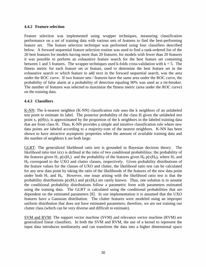
4.4.2 Feature selection .................................................................................................. 30

4.4.3 Classifiers ............................................................................................................ 30

4.4.4 Training Labels and Types .................................................................................. 31

5. Results and Discussion ..................................................................................................... 34

5.1 Performance Statistics – all UXO and all non-UXO...................................................... 35

5.2 ROC Performance as a function of Classifier ................................................................ 36

iii

5.3 Performance as a function of Data/Model...................................................................... 37

5.4 Inverted Features ............................................................................................................ 38

5.5 All UXO versus all non-UXO Results Summary........................................................... 40

5.6 Subgroups based on Size ................................................................................................ 40

5.7 Performance Bounds ...................................................................................................... 43

5.8 Comparison of Dynamic versus Static Data Collection ................................................. 45

5.9 Discussion ...................................................................................................................... 52

6. Conclusions and Implications for Future Research/Implementation ................................ 52

iv

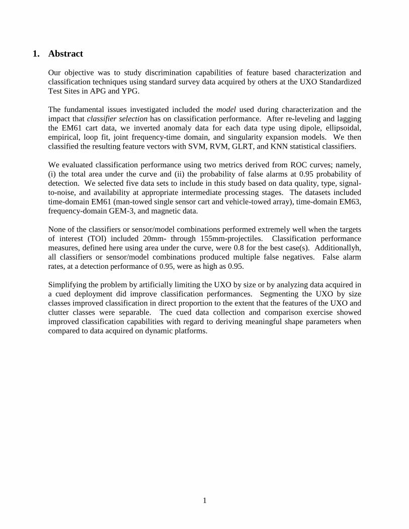
Figures Figure 3-1 Composite image of Aberdeen Proving Ground, MD, as configured while the data analyzed in this study was collected. .............................................................................................. 3

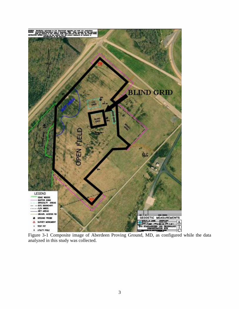
Figure 3-2 Photographs of standardized UXO emplaced at APG and YPG................................... 4

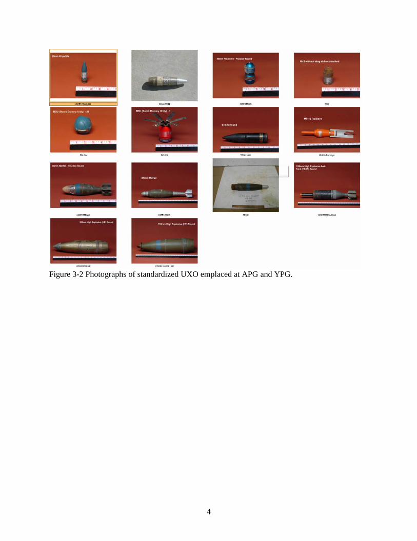
Figure 3-3 Photographs of example clutter emplaced at APG and YPG. A significant fraction of the clutter items included in this study was medium to large fragments and possessed thick walls.......................................................................................................................................................... 5

Figure 4-1 MTADS tow vehicle and magnetometer array ............................................................. 7

Figure 4-2 MTADS EM61 array pulled by the MTADS tow vehicle. ........................................... 8

Figure 4-3 Close-up of MTADS EM61 array with GPS and IMU. ................................................ 8

Figure 4-4 MTADS GEM array mounted on the EM sensor cart. In addition to the three GEM sensors, note the three GPS antennae and the IMU for platform motion measurement. ................ 9

Figure 4-5 Photograph of the EM63 sensor during data acquisition by the demonstrator. .......... 10

Figure 4-6 Photograph of the man-portable EM61 sensor during acquisition at APG. ................ 11

Figure 4-7 Example data from a small portion of APG open field. The superimposed symbols and text identify anomalies for which ground truth has been released. The grid lines are spaced 25m apart. ..................................................................................................................................... 12

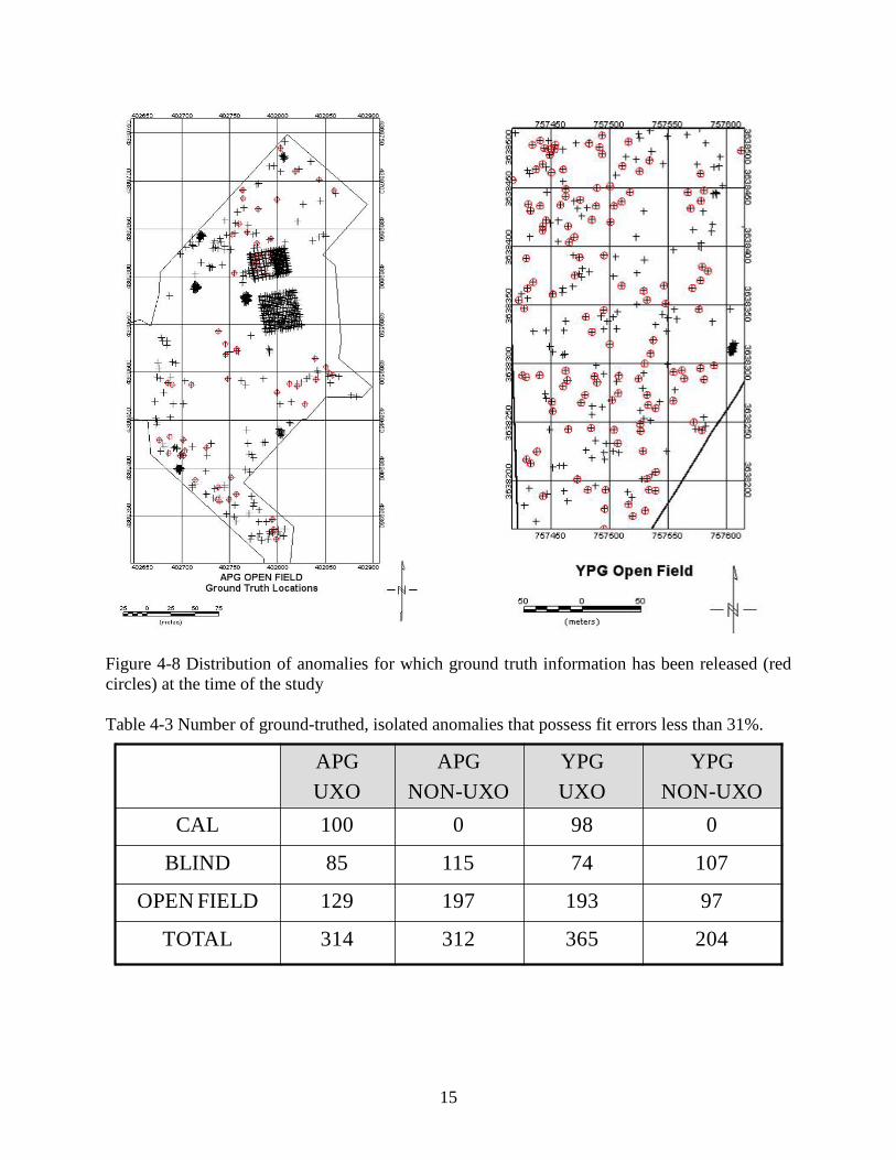
Figure 4-8 Distribution of anomalies for which ground truth information has been released (red circles) at the time of the study ..................................................................................................... 15

Figure 4-9 Fitted features derived from the NRL EM61 training data, YPG site, fit errors less than 31%. ...................................................................................................................................... 17

Figure 4-10 Fitted features derived from the TTFW EM61 training data, YPG site, fit errors less than 31%. ...................................................................................................................................... 18

Figure 4-11 Fitted features derived from the WES EM63 training data, YPG site, fit errors less than 31%. ...................................................................................................................................... 20

Figure 4-12 Empirical fitted features derived from the NRL GEM-3 training data, YPG site, fit errors less than 31%. ..................................................................................................................... 22

Figure 4-13 Ellipsoidal scale fitted features derived from the NRL GEM-3 training data, YPG site, fit errors less than 31%. ......................................................................................................... 24

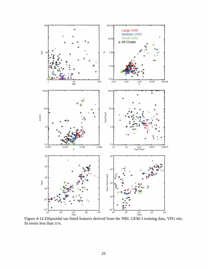
Figure 4-14 Ellipsoidal tau fitted features derived from the NRL GEM-3 training data, YPG site, fit errors less than 31%. ................................................................................................................ 25

Figure 4-15 Actual versus estimated depth and size plots and other relevant features plots; NRL magnetic array data, YPG open field ............................................................................................ 28

Figure 4-16 Classification ROCs for different scenarios of training and test data sets ................ 32

Figure 4-17 Type and number of training labels available for this study. As used here, ‘NS’ indicates non-standard munitions. All other notations are specific subtypes of a particular munition type. ............................................................................................................................... 33

v

Figure 5-1 Schematic showing the forward sequential feature selection process adopted for identifying the best performing set of features for each combination of data type and model. ... 34

Figure 5-2 Comparison of hypothetical ROC curves possessing specific AUC measures ........... 34

Figure 5-3 Performance ROCs as a function of classifiers for specific data types and best performing model.......................................................................................................................... 36

Figure 5-4 Performance ROCs for specific data types and models as detailed in the key. .......... 37

Figure 5-5 Inverted model features for EM63 data ...................................................................... 38

Figure 5-6 Inverted model features for EM61 data ...................................................................... 39

Figure 5-7 Inverted model features for magnetic data .................................................................. 40

Figure 5-8 Performance ROCs for size based scenarios versus all clutter ................................... 41

Figure 5-9 Performance ROCs by data type for Large UXO versus small clutter; KNN classifier....................................................................................................................................................... 42

Figure 5-10 Performance ROCs by data type for Large UXO versus small and medium sized clutter; KNN classifier .................................................................................................................. 43

Figure 5-11 Performance bounds assuming inverted features duplicate the observed physical dimensions of length and width (assumed to be equal to the diameter for axial symmetric UXO). Left column – inverted polarization features. Ground Truth (GT) dimensions as reported. Right side – ROC generated by submitting the length and width data to a KNN classifier. .................. 44

Figure 5-12 Photographs of three different collection schemes compared in this section. Top left shows a cued deployment using a fixed sampling scheme. Top right shows the TEMTADS vehicular array. Bottom left shows a man-towed deployment scheme. ...................................... 45

Figure 5-13 Comparison of dipole fit errors for common anomalies at APG with an EM61 sensor using a template, cart, and vehicular array deployment................................................................ 46

Figure 5-14 Similar errors in reported depth estimates are observed for the three deployment schemes; labeled UXO only.......................................................................................................... 47

Figure 5-15 Polarization shape comparison plots (principal axis B1 compared to second/tertiary B2,B3 polarizations) ..................................................................................................................... 48

Figure 5-16 Performance ROCs for template, cart, and vehicular array; EM61sensor, all UXO versus all clutter ............................................................................................................................ 49

Figure 5-17 Polarizations segmented by survey modality and target size .................................... 50

Figure 5-18 Performance ROCs for template, cart, and vehicular array; EM61sensor, sized based UXO classes versus all clutter ...................................................................................................... 51

Figure 7-1 ROC curves for NRL EM61 array data using the dipole model at YPG for different classifiers and features selection methodologies using features of anomalies with fit errors less than 31% . The targets of interest were all ordnance ranging from 20mm to 155mm. ............... 55

Figure 7-2 ROC curves for NRL EM61 array data using the dipole model at YPG for different classifiers and features selection methodologies using features of anomalies with fit errors less

vi

than 31% . The targets of interest were small sized ordnance items (20mm, 40mm, M42, BDU-28, BDU-26). ................................................................................................................................ 55

Figure 7-3 ROC curves for NRL EM61 array data using the dipole model at YPG for different classifiers and features selection methodologies using features of anomalies with fit errors less than 31% . The targets of interest were medium sized ordnance items (57mm, MK118, 60mm, 81mm, 2.75in). .............................................................................................................................. 56

Figure 7-4 ROC curves for NRL EM61 array data using the dipole model at YPG for different classifiers and features selection methodologies using features of anomalies with fit errors less than 31% . The targets of interest were large sized ordnance items (105mm, 155mm). ............. 56

Figure 7-5 ROC curves for TTFW EM61 cart data using the dipole model at YPG for different classifiers and features selection methodologies using features of anomalies with fit errors less than 31% . The targets of interest were all ordnance ranging from 20mm to 155mm. ............... 57

Figure 7-6 ROC curves for TTFW EM61 cart data using the dipole model at YPG for different classifiers and features selection methodologies using features of anomalies with fit errors less than 31% . The targets of interest were small sized ordnance items (20mm, 40mm, M42, BDU-28, BDU-26). ................................................................................................................................ 58

Figure 7-7 ROC curves for TTFW EM61 cart data using the dipole model at YPG for different classifiers and features selection methodologies using features of anomalies with fit errors less than 31% . The targets of interest were medium sized ordnance items (57mm, MK118, 60mm, 81mm, 2.75in). .............................................................................................................................. 58

Figure 7-8 ROC curves for TTFW EM61 cart data using the dipole model at YPG for different classifiers and features selection methodologies using features of anomalies with fit errors less than 31% . The targets of interest were large sized ordnance items (105mm, 155mm). ............. 59

Figure 7-9 ROC curves for NRL Mag array data at YPG for different classifiers and features selection methodologies using features of anomalies with fit errors less than 31% . The targets of interest were all ordnance ranging from 20mm to 155mm. ..................................................... 60

Figure 7-10 ROC curves for NRL Mag array data at YPG for different classifiers and features selection methodologies using features of anomalies with fit errors less than 31% . The targets of interest were small sized ordnance items (20mm, 40mm, M42, BDU-28, BDU-26). ............. 60

Figure 7-11 ROC curves for NRL Mag array data at YPG for different classifiers and features selection methodologies using features of anomalies with fit errors less than 31% . The targets of interest were medium sized ordnance items (57mm, MK118, 60mm, 81mm, 2.75in). ........... 61

Figure 7-12 ROC curves for NRL Mag array data at YPG for different classifiers and features selection methodologies using features of anomalies with fit errors less than 31% . The targets of interest were large sized ordnance items (105mm, 155mm). ................................................... 61

Figure 7-13 ROC curves for NRL array data using the cooperative Mag/EM approach at YPG for different classifiers and features selection methodologies using features of anomalies with fit errors less than 31% . The targets of interest were all ordnance ranging from 20mm to 155mm........................................................................................................................................................ 62

Figure 7-14 ROC curves for NRL array data using the cooperative Mag/EM approach at YPG for different classifiers and features selection methodologies using features of anomalies with fit

vii

errors less than 31% . The targets of interest were small sized ordnance items (20mm, 40mm, M42, BDU-28, BDU-26). ............................................................................................................. 63

Figure 7-15 ROC curves for NRL array data using the cooperative Mag/EM approach at YPG for different classifiers and features selection methodologies using features of anomalies with fit errors less than 31% . The targets of interest were medium sized ordnance items (57mm, MK118, 60mm, 81mm, 2.75in). ................................................................................................... 63

Figure 7-16 ROC curves for NRL array data using the cooperative Mag/EM approach at YPG for different classifiers and features selection methodologies using features of anomalies with fit errors less than 31% . The targets of interest were large sized ordnance items (105mm, 155mm)........................................................................................................................................................ 64

Figure 7-17 ROC curves for WES EM63 data using the POB model at YPG for different classifiers and features selection methodologies using features of anomalies with fit errors less than 31% . The targets of interest were all ordnance ranging from 20mm to 155mm. ............... 65

Figure 7-18 ROC curves for WES EM63 data using the POB model at YPG for different classifiers and features selection methodologies using features of anomalies with fit errors less than 31% . The targets of interest were small sized ordnance items (20mm, 40mm, M42, BDU-28, BDU-26). ................................................................................................................................ 65

Figure 7-19 ROC curves for WES EM63 data using the POB model at YPG for different classifiers and features selection methodologies using features of anomalies with fit errors less than 31% . The targets of interest were medium sized ordnance items (57mm, MK118, 60mm, 81mm, 2.75in). .............................................................................................................................. 66

Figure 7-20 ROC curves for WES EM63 using the POB model at YPG for different classifiers and features selection methodologies using features of anomalies with fit errors less than 31% . The targets of interest were large sized ordnance items (105mm, 155mm). ................................ 66

Figure 7-21 ROC curves for WES EM63 data using the SEM model at YPG for different classifiers and features selection methodologies using features of anomalies with fit errors less than 31% . The targets of interest were all ordnance ranging from 20mm to 155mm. ............... 67

Figure 7-22 ROC curves for WES EM63 data using the SEM model at YPG for different classifiers and features selection methodologies using features of anomalies with fit errors less than 31% . The targets of interest were small sized ordnance items (20mm, 40mm, M42, BDU-28, BDU-26). ................................................................................................................................ 68

Figure 7-23 ROC curves for WES EM63 data using the SEM model at YPG for different classifiers and features selection methodologies using features of anomalies with fit errors less than 31% . The targets of interest were medium sized ordnance items (57mm, MK118, 60mm, 81mm, 2.75in). .............................................................................................................................. 68

Figure 7-24 ROC curves for WES EM63 data using the SEM model at YPG for different classifiers and features selection methodologies using features of anomalies with fit errors less than 31% . The targets of interest were large sized ordnance items (105mm, 155mm). ............. 69

Figure 7-25 ROC curves for NRL GEM-3 array data using the ellipsoidal scale model at YPG for different classifiers and features selection methodologies using features of anomalies with fit errors less than 31% . The targets of interest were all ordnance ranging from 20mm to 155mm........................................................................................................................................................ 70

viii

Figure 7-26 ROC curves for NRL GEM-3 array data using the ellipsoidal scale model at YPG for different classifiers and features selection methodologies using features of anomalies with fit errors less than 31% . The targets of interest were small sized ordnance items (20mm, 40mm, M42, BDU-28, BDU-26). ............................................................................................................. 70

Figure 7-27 ROC curves for NRL GEM-3 array data using the ellipsoidal scale model at YPG for different classifiers and features selection methodologies using features of anomalies with fit errors less than 31% . The targets of interest were medium sized ordnance items (57mm, MK118, 60mm, 81mm, 2.75in). ................................................................................................... 71

Figure 7-28 ROC curves for NRL GEM-3 array data using the ellipsoidal scale model at YPG for different classifiers and features selection methodologies using features of anomalies with fit errors less than 31% . The targets of interest were large sized ordnance items (105mm, 155mm)........................................................................................................................................................ 71

Figure 7-29 ROC curves for NRL GEM-3 array data using the ellipsoidal tau model at YPG for different classifiers and features selection methodologies using features of anomalies with fit errors less than 31% . The targets of interest were all ordnance ranging from 20mm to 155mm........................................................................................................................................................ 72

Figure 7-30 ROC curves for NRL GEM-3 array data using the ellipsoidal tau model at YPG for different classifiers and features selection methodologies using features of anomalies with fit errors less than 31% . The targets of interest were small sized ordnance items (20mm, 40mm, M42, BDU-28, BDU-26). ............................................................................................................. 73

Figure 7-31 ROC curves for NRL GEM-3 array data using the ellipsoidal tau model at YPG for different classifiers and features selection methodologies using features of anomalies with fit errors less than 31% . The targets of interest were medium sized ordnance items (57mm, MK118, 60mm, 81mm, 2.75in). ................................................................................................... 73

Figure 7-32 ROC curves for NRL GEM-3 array data using the ellipsoidal tau model at YPG for different classifiers and features selection methodologies using features of anomalies with fit errors less than 31% . The targets of interest were large sized ordnance items (105mm, 155mm)........................................................................................................................................................ 74

Figure 7-33 ROC curves for NRL GEM-3 array data using the empirical model at YPG for different classifiers and features selection methodologies using features of anomalies with fit errors less than 31% . The targets of interest were all ordnance ranging from 20mm to 155mm........................................................................................................................................................ 75

Figure 7-34 ROC curves for NRL GEM-3 array data using the empirical model at YPG for different classifiers and features selection methodologies using features of anomalies with fit errors less than 31% . The targets of interest were small sized ordnance items (20mm, 40mm, M42, BDU-28, BDU-26). ............................................................................................................. 75

Figure 7-35 ROC curves for NRL GEM-3 array data using the empirical model at YPG for different classifiers and features selection methodologies using features of anomalies with fit errors less than 31% . The targets of interest were medium sized ordnance items (57mm, MK118, 60mm, 81mm, 2.75in). ................................................................................................... 76

Figure 7-36 ROC curves for NRL GEM-3 array data using the empirical model at YPG for different classifiers and features selection methodologies using features of anomalies with fit

ix

errors less than 31% . The targets of interest were large sized ordnance items (105mm, 155mm)........................................................................................................................................................ 76

Figure 7-37 ROC curves for NRL GEM-3 array data using the loop model at YPG for different classifiers and features selection methodologies using features of anomalies with fit errors less than 31% . The targets of interest were all ordnance ranging from 20mm to 155mm. ............... 78

Figure 7-38 ROC curves for NRL GEM-3 array data using the loop model at YPG for different classifiers and features selection methodologies using features of anomalies with fit errors less than 31% . The targets of interest were small sized ordnance items (20mm, 40mm, M42, BDU-28, BDU-26). ................................................................................................................................ 78

Figure 7-39 ROC curves for NRL GEM-3 array data using the loop model at YPG for different classifiers and features selection methodologies using features of anomalies with fit errors less than 31% . The targets of interest were medium sized ordnance items (57mm, MK118, 60mm, 81mm, 2.75in). .............................................................................................................................. 79

Figure 7-40 ROC curves for NRL GEM-3 array data using the loop model at YPG for different classifiers and features selection methodologies using features of anomalies with fit errors less than 31% . The targets of interest were large sized ordnance items (105mm, 155mm). ............. 79

Tables Table 4-1 Datasets included in this study ....................................................................................... 6

Table 4-2 NRL EM61 Gate timing parameters ............................................................................... 7

Table 4-3 Number of ground-truthed, isolated anomalies that possess fit errors less than 31%. . 15

Table 5-1 Performance Measures as a function of Data and Model ............................................. 35

Table 5-2 Performance Measures for EM61, Mag, and EM63 data types ................................... 37

Table 5-3 Size based definitions of UXO and clutter ................................................................... 41

Table 5-4 Sample size for various combinations of UXO and clutter .......................................... 41

Table 5-5 Inverted fit statistics ..................................................................................................... 46

Table 7-1 Best set of features for each of the classifiers with different TOI using the NRL EM61 array data at YPG. ......................................................................................................................... 54

Table 7-2 Best set of features for each of the classifiers with different TOI using the TTFW EM61 cart data at YPG. ................................................................................................................ 57

Table 7-3 Best set of features for each of the classifiers with different TOI using the NRL Mag array data at YPG. ......................................................................................................................... 59

Table 7-4 Best set of features for each of the classifiers with different TOI using the NRL EM61 and Mag array data and the cooperative inversion approach at YPG. .......................................... 62

Table 7-5 Best set of features for each of the classifiers with different TOI using the WES EM63 data and the POB model at YPG................................................................................................... 64

x

Table 7-6 Best set of features for each of the classifiers with different TOI using the WES EM63 data and the SEM model at YPG. ................................................................................................. 67

Table 7-7 Best set of features for each of the classifiers with different TOI using the NRL GEM-3 array and the ellipsoidal scale model at YPG. ........................................................................... 69

Table 7-8 Best set of features for each of the classifiers with different TOI using the NRL GEM-3 array data and the ellipsoidal tau model at YPG. ....................................................................... 72

Table 7-9 Best set of features for each of the classifiers with different TOI using the NRL GEM-3 array data and the empirical model at YPG. .............................................................................. 74

Table 7-10 Best set of features for each of the classifiers with different TOI using the NRL GEM-3 array data and the loop model at YPG. ............................................................................ 77

Acknowledgements This report was supported wholly by the U.S. Department of Defense, through the Strategic Environmental Research and Development Program (SERDP) through Project MM-1505.

xi

List of Acronyms AEC Army Environmental Center

ASR Archives Search Report

APG Aberdeen Proving Ground

BD Bhattacharyya Distance

BoR Body of Rotation

DAQ Data Acquisition

DGM Digital Geophysical Mapping

DSB Defense Science Board

EE/CA Engineering Evaluation/Cost Analysis

EMI Electromagnetic Induction

ESTCP Environmental Security Technology Certification Program

FAR False Alarm Rate

FD Frequency domain

FLD Fisher Linear Discriminant

FSS Forward Sequential Selection

GLRT Generalized Likelihood Ratio Test

GPO Geophysical Prove Out

GPS Global Positioning System

HE High Explosive

IDA Institute for Defense Analyses

IMU Inertial Measurement Unit

KDE Kernel Density Estimation

K-NN K-nearest neighbor

LSQ Least Squares

M&F Mag and Flag

MR Munitions Response

MTADS Multi-sensor Towed Array Detection System

NRL Naval Research Laboratory

Pd Probability of Detection

xii

Pdisc Probability of Correct Discrimination

Pfa Probability of False Alarm

POB Pasion-Oldenburg-Billings

QA Quality Assurance

QC Quality Control

ROC Receiver Operating Characteristic

RTK Real Time Kinematic

RTS Robotic Total Station

RVM Relevance Vector Machine

SEM Singularity Expansion Model

SERDP Strategic Environmental Research and Development Program

SNR Signal to Noise Ratio

SPRT Statistical Pattern Recognition Toolbox

SVM Support Vector Machine

TD Time domain

TtFW TetraTech Foster Wheeler

TOI Target(s) of Interest

UTC Coordinated Universal Time

UXO Unexploded Ordnance

VB Variational Bayes

WES Waterways Experiment Station

YPG Yuma Proving Ground

1

1. Abstract Our objective was to study discrimination capabilities of feature based characterization and classification techniques using standard survey data acquired by others at the UXO Standardized Test Sites in APG and YPG. The fundamental issues investigated included the model used during characterization and the impact that classifier selection has on classification performance. After re-leveling and lagging the EM61 cart data, we inverted anomaly data for each data type using dipole, ellipsoidal, empirical, loop fit, joint frequency-time domain, and singularity expansion models. We then classified the resulting feature vectors with SVM, RVM, GLRT, and KNN statistical classifiers. We evaluated classification performance using two metrics derived from ROC curves; namely, (i) the total area under the curve and (ii) the probability of false alarms at 0.95 probability of detection. We selected five data sets to include in this study based on data quality, type, signal-to-noise, and availability at appropriate intermediate processing stages. The datasets included time-domain EM61 (man-towed single sensor cart and vehicle-towed array), time-domain EM63, frequency-domain GEM-3, and magnetic data. None of the classifiers or sensor/model combinations performed extremely well when the targets of interest (TOI) included 20mm- through 155mm-projectiles. Classification performance measures, defined here using area under the curve, were 0.8 for the best case(s). Additionallyh, all classifiers or sensor/model combinations produced multiple false negatives. False alarm rates, at a detection performance of 0.95, were as high as 0.95. Simplifying the problem by artificially limiting the UXO by size or by analyzing data acquired in a cued deployment did improve classification performances. Segmenting the UXO by size classes improved classification in direct proportion to the extent that the features of the UXO and clutter classes were separable. The cued data collection and comparison exercise showed improved classification capabilities with regard to deriving meaningful shape parameters when compared to data acquired on dynamic platforms.

2

2. Objective The objective of this project was to evaluate and improve physics-inspired discrimination performances by systematically scrutinizing the process; namely, the model used during characterization and the impact that classifier selection and training has on the final decision.

3. Background The UXO Standardized Test Sites in Aberdeen Maryland and Yuma Arizona represent real world scenarios (Figure 3-1). They were established under SERDP, ESTCP, and Army funding to allow users and developers to baseline and document UXO technology performance by defining the range of applicability of specific UXO technologies, by gathering data on sensor and system performance, and by comparing results. Electromagnetic and magnetic data acquired at these sites over multiple years and by multiple firms provided an opportunity to systematically examine the importance of models, classifiers, and training data when trying to discriminate between UXO and clutter using remotely sensed geophysical data. The UXO Standardized Test Site program was designed to benchmark and validate capabilities of service firms and research groups. Technology demonstrators were free to choose the geophysical sensor, the positioning system, ancillary orientation sensors, deployment method, and analysis method. Approximately two dozen collections of digital geophysical data were collected, within at least a portion of the sites, from 2002 thru 2006. Most of the demonstrators’ utilized magnetic or electromagnetic sensors of one kind or another (only one firm demonstrated a Ground Penetrating Radar technology). The government scored the demonstrator submittals by using various quantitative metrics aimed at deciphering how well they detected subsurface metallic objects and discriminated UXO from non-UXO metallic debris. Performance results released by the Army Environmental Center (AEC) were generally poor. Based on AEC reports, in fact, little to no discernible discrimination capabilities were demonstrated using survey data [1]. This project investigated whether advanced signal processing and quantitative decision processes would improve the discrimination results.

3

Figure 3-1 Composite image of Aberdeen Proving Ground, MD, as configured while the data analyzed in this study was collected.

4

Figure 3-2 Photographs of standardized UXO emplaced at APG and YPG.

5

Figure 3-3 Photographs of example clutter emplaced at APG and YPG. A significant fraction of the clutter items included in this study was medium to large fragments and possessed thick walls.

6

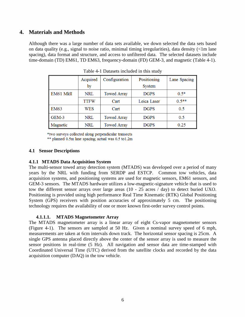
4. Materials and Methods Although there was a large number of data sets available, we down selected the data sets based on data quality (e.g., signal to noise ratio, minimal timing irregularities), data density (<1m lane spacing), data format and structure, and access to unfiltered data. The selected datasets include time-domain (TD) EM61, TD EM63, frequency-domain (FD) GEM-3, and magnetic (Table 4-1).

Table 4-1 Datasets included in this study

4.1 Sensor Descriptions 4.1.1 MTADS Data Acquisition System The multi-sensor towed array detection system (MTADS) was developed over a period of many years by the NRL with funding from SERDP and ESTCP. Common tow vehicles, data acquisition systems, and positioning systems are used for magnetic sensors, EM61 sensors, and GEM-3 sensors. The MTADS hardware utilizes a low-magnetic-signature vehicle that is used to tow the different sensor arrays over large areas (10 - 25 acres / day) to detect buried UXO. Positioning is provided using high performance Real Time Kinematic (RTK) Global Positioning System (GPS) receivers with position accuracies of approximately 5 cm. The positioning technology requires the availability of one or more known first-order survey control points.

4.1.1.1. MTADS Magnetometer Array The MTADS magnetometer array is a linear array of eight Cs-vapor magnetometer sensors (Figure 4-1). The sensors are sampled at 50 Hz. Given a nominal survey speed of 6 mph, measurements are taken at 6cm intervals down track. The horizontal sensor spacing is 25cm. A single GPS antenna placed directly above the center of the sensor array is used to measure the sensor positions in real-time (5 Hz). All navigation and sensor data are time-stamped with Coordinated Universal Time (UTC) derived from the satellite clocks and recorded by the data acquisition computer (DAQ) in the tow vehicle.

7

See AEC standardized scoring report #671 for more information regarding this system as deployed at APG [http://aec.army.mil/usaec/technology/demosites/sr0671.pdf].

Figure 4-1 MTADS tow vehicle and magnetometer array

4.1.1.2. MTADS EM61 Array The EM61 MTADS array is an overlapping array of three pulsed-induction sensors with 1x1m coils. The sensors have been modified to make them more compatible with vehicular speeds and to increase their sensitivity to small objects (Table 4-2). Nominal survey speed is three mph and the sensor readings are recorded at 10 Hz. This results in a down-track sampling of ~15 cm and a cross-track interval of 50 cm. In order to obtain sufficient illumination of all three principle axes of the anomaly with the primary field, data is collected in two orthogonal surveys. The EM61 array being pulled by the MTADS tow vehicle is shown in Figure 4-2. Individual sensors in the EM61 array are located using a three-receiver RTK GPS system. An Inertial Measurement Unit (IMU) is also included on the sensor array to provide complimentary platform orientation information. A close-up view of the sensor platform is shown in Figure 4-3 which shows the three GPS antennae and the IMU (black box under the aft port GPS antenna).

Table 4-2 NRL EM61 Gate timing parameters Delay (µs)

4 Gate Mode Delay (µs) Differential Mode

Gate 1 307 (bottom coil) 307 (bottom coil) Gate 2 508 (bottom coil) 307 (top coil) Gate 3 738 (bottom coil) 738 (bottom coil) Gate 4 1000 (bottom coil) 1000 (bottom coil)

8

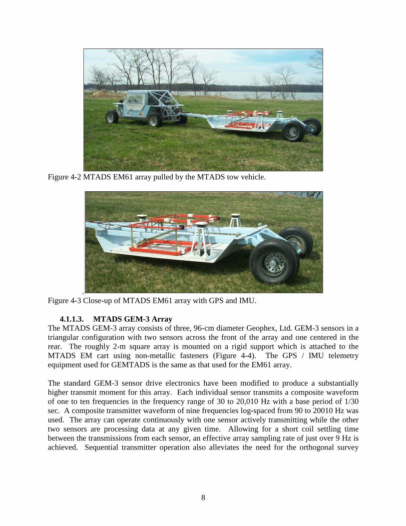
Figure 4-2 MTADS EM61 array pulled by the MTADS tow vehicle.

. Figure 4-3 Close-up of MTADS EM61 array with GPS and IMU.

4.1.1.3. MTADS GEM-3 Array The MTADS GEM-3 array consists of three, 96-cm diameter Geophex, Ltd. GEM-3 sensors in a triangular configuration with two sensors across the front of the array and one centered in the rear. The roughly 2-m square array is mounted on a rigid support which is attached to the MTADS EM cart using non-metallic fasteners (Figure 4-4). The GPS / IMU telemetry equipment used for GEMTADS is the same as that used for the EM61 array. The standard GEM-3 sensor drive electronics have been modified to produce a substantially higher transmit moment for this array. Each individual sensor transmits a composite waveform of one to ten frequencies in the frequency range of 30 to 20,010 Hz with a base period of 1/30 sec. A composite transmitter waveform of nine frequencies log-spaced from 90 to 20010 Hz was used. The array can operate continuously with one sensor actively transmitting while the other two sensors are processing data at any given time. Allowing for a short coil settling time between the transmissions from each sensor, an effective array sampling rate of just over 9 Hz is achieved. Sequential transmitter operation also alleviates the need for the orthogonal survey

9

mode employed for the EM61 array. Down-track sampling is approximately 15 cm and the cross-track spacing is 50 cm. An interleaved survey pattern is used to decrease the cross-track spacing to 25 cm. See AEC standardized scoring report #127 for more information regarding this system as deployed at APG [http://aec.army.mil/usaec/technology/demosites/sr0127.pdf].

Figure 4-4 MTADS GEM array mounted on the EM sensor cart. In addition to the three GEM sensors, note the three GPS antennae and the IMU for platform motion measurement. 4.1.2 EM63 man-portable The EM63 is a commercially available sensor produced by Geonics, Ltd., of Mississauga, Ontario, Canada (Figure 4-5). It is a high power, high sensitivity, wide bandwidth full time domain UXO detector. The EM63 consists of a transmitter that generates a pulsed primary magnetic field which induces eddy currents in nearby metallic objects. The time decay of the currents is measured and recorded by the main console at 20 to 30 geometrically spaced time gates covering a time range from 180 microseconds (μs) to 63 milliseconds (ms). The EM63 system consists of three major hardware subsystems: (i) EM63 Control Console Sub-System; (ii) Antenna Cart Sub-System; and (iii) GPS Navigation Sub-System. The EM63 Control Console Sub-System consists of receiver and transmitter unit, controlled by an integrated field computer. The Antenna Cart Sub-System consists of the transmitter antenna (the 1x1m bottom coil) and receiver coils. Local positioning and georeferencing was accomplished using a Trimble 5700 RTK GPS system. The Trimble system consists of two receivers that are in radio communication with each other. A roving GPS antenna is mounted in the center of the EM63 coils and 2 meters above the bottom coil. The operator or assistant carries the controller for the roving antenna.

10

See AEC standardized scoring report #304 for more information regarding this system as deployed at APG [http://aec.army.mil/usaec/technology/demosites/sr0304.pdf].

Figure 4-5 Photograph of the EM63 sensor during data acquisition by the demonstrator. 4.1.3 EM61 man-portable The Geonics EM61 TDEM geophysical sensor, Arc Second Constellation, and Leica Series 1100 Robotic Total Station laser positioning systems were integrated into a man-towed sensing system by TtFW (Figure 4-6). The system is utilized either on nonmagnetic wheels or as a man-portable unit (terrain-dependent) with the lower coil 40 cm above the ground surface. Two coils, 1x1m, are oriented in a horizontal coplanar fashion and separated by a vertical distance of 40 cm. The secondary magnetic field created by metal objects is sampled by the EM61 electronics, which reside in the backpack, at times of 216 μs, 366 μs, 660 μs on the bottom coil and 660 μs on the top coil after the turn-off of the transmit pulse. Digital data for these four individual time gates are integrated and recorded to a Juniper Allegro field computer at a rate of 12 Hz. The Arc Second Constellation consists of four laser transmitters and a field computer for logging the position data via wireless modem. Four Trimble Spectra Precision LS920 Laser Transmitters are positioned in a diamond or square geometry over 1/2 to 1 acre depending upon the tree density. The transmitters are leveled, and an automatic routine calculates the relative x-y-z- plane between the transmitters to a tolerance of 1 inch or less. A laser detector receiver is centered over the EM61 coils on a TtFW designed fiberglass doghouse. The detector wand receives the laser pulses from the four transmitters simultaneously, and computes a position based on the known position of the laser transmitters. The georeferenced data are updated at 2 to 3 Hz and sent via wireless modem to the field computer for storage. The Leica Series 1100 RTS consists of a laser-based total station survey instrument (transmitter), prism (receiver), and RCS 100 remote control. The receiver prism is mounted on a TtFW doghouse centered over the EM61 coils, and the RTS automatically tracks the prism at distances of several thousand feet to

11

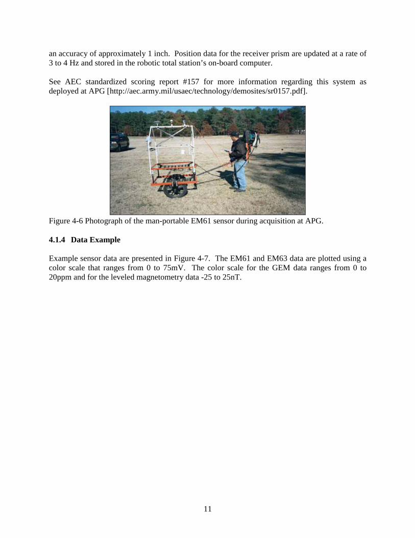
an accuracy of approximately 1 inch. Position data for the receiver prism are updated at a rate of 3 to 4 Hz and stored in the robotic total station’s on-board computer. See AEC standardized scoring report #157 for more information regarding this system as deployed at APG [http://aec.army.mil/usaec/technology/demosites/sr0157.pdf].

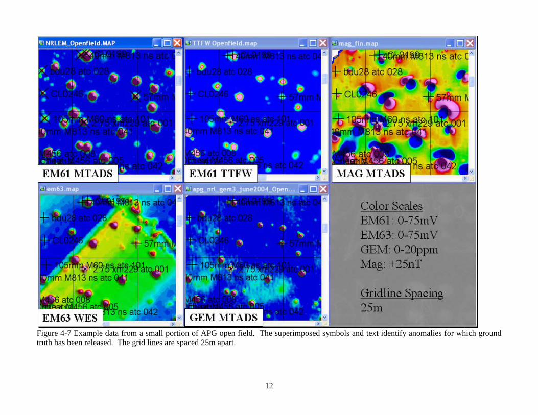
Figure 4-6 Photograph of the man-portable EM61 sensor during acquisition at APG. 4.1.4 Data Example Example sensor data are presented in Figure 4-7. The EM61 and EM63 data are plotted using a color scale that ranges from 0 to 75mV. The color scale for the GEM data ranges from 0 to 20ppm and for the leveled magnetometry data -25 to 25nT.

12

Figure 4-7 Example data from a small portion of APG open field. The superimposed symbols and text identify anomalies for which ground truth has been released. The grid lines are spaced 25m apart.

13

4.2 Anomalies of Opportunity Only a subset of the total number of targets emplaced at the test sites were suitable for inclusion in this study. First, in order to compare methods and/or data sets, we required ground truth information. Ground truth information was available for anomalies in the calibration grid, original blind grid, and some of the open field challenge area at the time that this project was active. Not all of the ground truthed targets, however, were suitable for use in this study. The reasons for ground truth release, in fact, included those targets that were ‘least found’, ‘never found’, ‘miscellaneous’, ‘near fence’, and as well as ‘misclassified’. Thus, of the 327 APG open field targets for which ground truth was released, 112 of them were not suitable. At YPG, approximately 50 of the released ground truthed anomalies were not suitable. To be included in this study, the anomalies also had to be common across the data sets and well characterized by the models. Table 4-3 presents the total number of isolated anomalies that possess correlation coefficients between measured and modeled data of greater than 0.95, which corresponds to fit errors less than 31%, for APG and YPG while Figure 4-8 shows the spatial distribution. We selected a 0.95 correlation coefficient threshold because fits with lower correlations possessed inconsistent polarizations and depth estimates across the models tested. 4.3 Data Models 4.3.1 Dipole Model Within the dipole model framework, each target is completely characterized by three positional parameters (xo,yo,zo), three angles (φ,θ,ψ), and three*Nt betas [β1(ti), β2(ti), β3(ti)], where Nt is the number of time gates. The β’s are eigenvalues of the symmetric effective magnetic polarizability tensor, and represent the response of the target along each of three principal axes. In order to reduce the number of fit parameters, we made use of the fact that the modeled sensor response is linear in the β’s. We therefore performed a non-linear Levenberg-Marquardt inversion on the positional and orientation parameters, with an embedded linear determination of the β’s at each iteration. The algorithm continued until the squared error between measured and modeled data (chi-squared or χ2) fit between the predicted and measured response at successive iterations changes by less than a set tolerance. Initial guesses were provided for the six spatial parameters. The three angles were set equal to 45 degrees. The positional parameters xo and yo were determined from a signal-weighted mean of the target locations. Previous experience with this method indicated that the final results were most strongly dependent on zo, as some guesses could lead to local minima. The code therefore was set to loop over several different initial guesses for zo that covered a reasonable range for the targets. The result with the best χ2 was chosen as the solution.

14

15

Figure 4-8 Distribution of anomalies for which ground truth information has been released (red circles) at the time of the study Table 4-3 Number of ground-truthed, isolated anomalies that possess fit errors less than 31%.

APGUXO

APGNON-UXO

YPGUXO

YPGNON-UXO

CAL 100 0 98 0

BLIND 85 115 74 107

OPEN FIELD 129 197 193 97

TOTAL 314 312 365 204

16

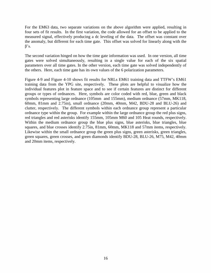
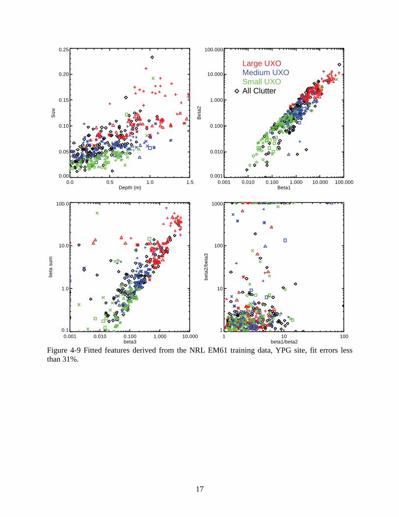
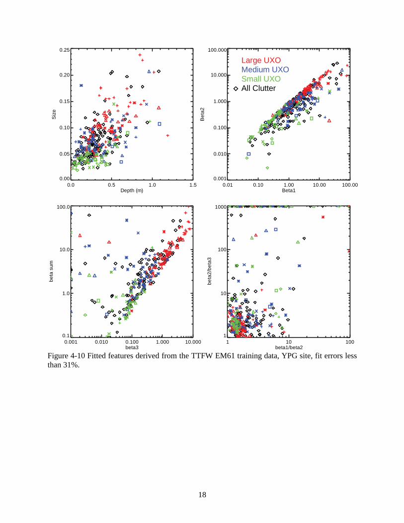
For the EM63 data, two separate variations on the above algorithm were applied, resulting in four sets of fit results. In the first variation, the code allowed for an offset to be applied to the measured signal, effectively producing a dc leveling of the data. The offset was constant over the anomaly, but different for each time gate. This offset was solved for linearly along with the β’s. The second variation hinged on how the time gate information was used. In one version, all time gates were solved simultaneously, resulting in a single value for each of the six spatial parameters over all time gates. In the other version, each time gate was solved independently of the others. Here, each time gate has its own values of the 6 polarization parameters. Figure 4-9 and Figure 4-10 shows fit results for NRLs EM61 training data and TTFW’s EM61 training data from the YPG site, respectively. These plots are helpful to visualize how the individual features plot in feature space and to see if certain features are distinct for different groups or types of ordnances. Here, symbols are color coded with red, blue, green and black symbols representing large ordnance (105mm and 155mm), medium ordnance (57mm, MK118, 60mm, 81mm and 2.75in), small ordnance (20mm, 40mm, M42, BDU-28 and BLU-26) and clutter, respectively. The different symbols within each ordnance group represent a particular ordnance type within the group. For example within the large ordnance group the red plus signs, red triangles and red asterisks identify 155mm, 105mm M60 and 105 Heat rounds, respectively. Within the medium ordnance group the blue plus signs, blue asterisks, blue triangles, blue squares, and blue crosses identify 2.75in, 81mm, 60mm, MK118 and 57mm items, respectively. Likewise within the small ordnance group the green plus signs, green asterisks, green triangles, green squares, green crosses, and green diamonds identify BDU-28, BLU-26, M75, M42, 40mm and 20mm items, respectively.

17

Figure 4-9 Fitted features derived from the NRL EM61 training data, YPG site, fit errors less than 31%.

0.0 0.5 1.0 1.5Depth (m)

0.00

0.05

0.10

0.15

0.20

0.25S

ize

0.001 0.010 0.100 1.000 10.000 100.000Beta1

0.001

0.010

0.100

1.000

10.000

100.000

Bet

a2

0.001 0.010 0.100 1.000 10.000beta3

0.1

1.0

10.0

100.0

beta

sum

1 10 100beta1/beta2

1

10

100

1000be

ta2/

beta

3

All ClutterSmall UXOMedium UXOLarge UXO

18

Figure 4-10 Fitted features derived from the TTFW EM61 training data, YPG site, fit errors less than 31%.

0.0 0.5 1.0 1.5Depth (m)

0.00

0.05

0.10

0.15

0.20

0.25S

ize

0.01 0.10 1.00 10.00 100.00Beta1

0.001

0.010

0.100

1.000

10.000

100.000

Bet

a2

0.001 0.010 0.100 1.000 10.000beta3

0.1

1.0

10.0

100.0

beta

sum

1 10 100beta1/beta2

1

10

100

1000be

ta2/

beta

3


19

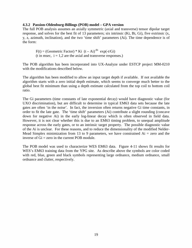
4.3.2 Passion-Oldenburg-Billings (POB) model – GPA version The full POB analysis assumes an axially symmetric (axial and transverse) tensor dipolar target response, and solves for the best fit of 13 parameters; six intrinsic (Ki, Bi, Gi), five extrinsic (x, y, z, azimuth, inclination), and the two ‘time shift’ parameters (Ai). The time dependence is of the form: F(t) = (Geometric Factor) * Ki (t – Ai)-Bi exp(-t/Gi) (t in msec, i = 1,2 are the axial and transverse responses.) The POB algorithm has been incorporated into UX-Analyze under ESTCP project MM-0210 with the modifications described below. The algorithm has been modified to allow an input target depth if available. If not available the algorithm starts with a zero initial depth estimate, which seems to converge much better to the global best fit minimum than using a depth estimate calculated from the top coil to bottom coil ratio. The Gi parameters (time constants of late exponential decay) would have diagnostic value (for UXO discrimination), but are difficult to determine in typical EM63 data sets because the late gates are often ‘in the noise’. In fact, the inversion often returns negative Gi time constants, in order to fit the late gate. The ‘time shift’ parameters (Ai) contribute a slight rounding (concave down for negative Ai) in the early log-linear decay which is often observed in field data. However, it is not clear whether this is due to an EM63 timing problem, to unequal amplitude response across the early gates, or to an intrinsic target property. The possible diagnostic value of the Ai is unclear. For these reasons, and to reduce the dimensionality of the modified Nelder-Mead Simplex minimization from 13 to 9 parameters, we have constrained Ai = zero and the inverse of Gi = zero in the current POB module. The POB model was used to characterize WES EM63 data. Figure 4-11 shows fit results for WES’s EM63 training data from the YPG site. As describe above the symbols are color coded with red, blue, green and black symbols representing large ordnance, medium ordnance, small ordnance and clutter, respectively.

20

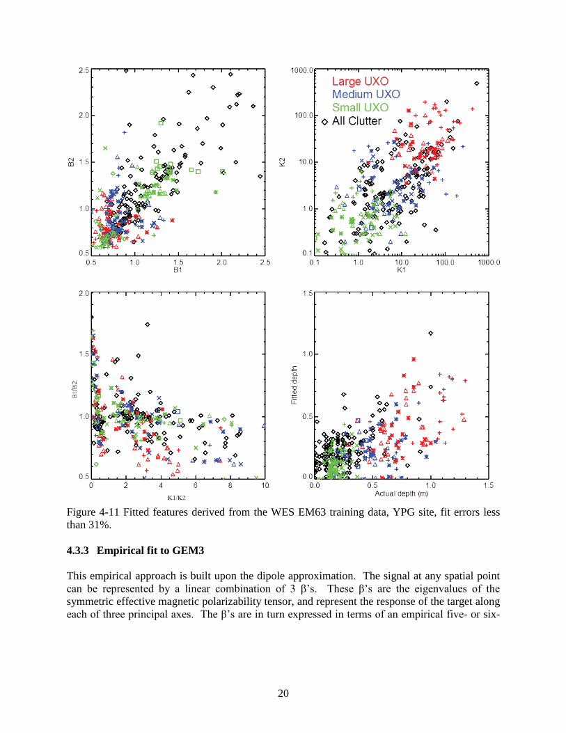
Figure 4-11 Fitted features derived from the WES EM63 training data, YPG site, fit errors less than 31%. 4.3.3 Empirical fit to GEM3 This empirical approach is built upon the dipole approximation. The signal at any spatial point can be represented by a linear combination of 3 β’s. These β’s are the eigenvalues of the symmetric effective magnetic polarizability tensor, and represent the response of the target along each of three principal axes. The β’s are in turn expressed in terms of an empirical five- or six-

21

parameter model [2]. This model is based on the theoretical responses of spheres and cylinders and has been shown empirically to fit a wide range of objects. The parameters of this model are τ, a time constant; A, an amplitude parameter; and S, f, and ν, shape parameters. In all, there are 18 features reported: 6 each from 3 principal axes. These features represent non-physical fit parameters from a frequency domain response model. Parameters are recovered in a two-stage process: (1) target position and orientation are determined through standard dipole-model inversion; (2) A 6 parameter FD response model is fit separately to observed beta response values, jβ , of each principal axis, which resulted from step (1). The 6 parameter model is:

τωαα

ααβν

ν igSgfgfA

C

j ==

+

+−

= + ,)(I

)(I,11 1

2

,

where fitted parameters S, f, C, and ν are dimensionless, while parameter A has dimension of volume, and parameter τ has dimension of time [2]. The symbol Iν(α) is the Modified Bessel I function of order ν. All fitted parameters are real scalars. This model was derived from analytic solutions for the conducting loop, for spheres of arbitrary permeability, and for infinite cylinders illuminated transversely, also with arbitrary permeability. It provides exact matches to all of those analytic solutions through parameter adjustment, and also provides good matches to a wide range of irregularly shaped UXO. Figure 4-12 shows fit results for WES’s EM63 training data from the YPG site. As describe above the symbols are color coded with red, blue, green and black symbols representing large ordnance, medium ordnance, small ordnance and clutter, respectively.

22

Figure 4-12 Empirical fitted features derived from the NRL GEM-3 training data, YPG site, fit errors less than 31%.

0.01 0.10 1.00 10.00 100.00Beta1 B/Beta2 B

0.01

0.10

1.00

10.00

100.00

Bet

a1 T

/Bet

a2 T

-10 -5 0 5 10Beta1 S/Beta2 S

-10

-5

0

5

10

Bet

a2 S

/Bet

a3 S

1 10 100 1000 10000Amp sum

-4

-2

0

2

4

S s

um

0 1 2 3A sum

0.0

0.5

1.0

1.5

2.0

B s

um

-1.0 -0.5 0.0 0.5 1.0Beta2 S

-1.0

-0.5

0.0

0.5

1.0

Bet

a3 S


23

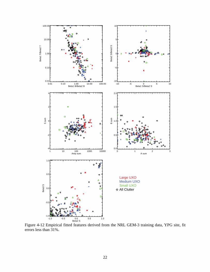
4.3.4 Ellipsoid Model Similar to the empirical model described in the previous section, the ellipsoid model used to invert the GEM-3 data was also built upon the dipole approximation. As before, the polarizations are first expressed in terms of an empirical 5- or 6-parameter model [2]. The parameters of this model are τ, a time constant; A, an amplitude parameter; and S, f, and ν, shape parameters. There are 3 sets of parameters per object, one for each principal axis. Here, in an effort to tie these parameters to actual physical dimensions we modeled the targets as ellipsoids. Assuming that the target is subjected to a uniform transmit field, the demagnetization factors can be expressed analytically in terms of A, b, and c, the semi-principal axes of the ellipsoid. This allows us to express the last four parameters in the empirical model in terms of a, b, c, and μr, the relative permeability of the target [3]. The remaining parameter, the τ’s, are handled by two different methods. In the first, the τ’s are simply treated as 3 independent fit parameters. In the second method, we make use of the fact that the τ’s scale as a size squared to tie them into the ellipsoidal semi-principal axes. By utilizing empirical measurements by Ben Barrowes [5], relating the ratio of the time constants to the ratio of ellipsoid sizes, we need add only one new fit parameter, a Scale factor relating a2 to τa. In summary, both inversion methods require 3 positional parameters (xo,yo,zo), 3 angles (φ,θ,ψ), the 3 ellipsoidal semi-principal axes (A,B,C), and the relative permeability of the target (μr). The first method then requires 3 τ’s, while the second requires only a scale factor. Initial guesses were provided for all parameters. The positional parameters xo and yo were determined from a signal-weighted mean of the target locations. The other parameters were set to reasonable values. With such a large number of parameters, ensuring that the inversion reaches the global minimum often requires a range of initial guesses for parameter values. In an effort to balance convergence to the global minimum with reasonable run time, we took the following approach. First, we perform multiple loops over the target depth and orientation (plus μr for the 3 τ method), but only allow for 5 iterations of the inversion routine. Whichever set of initial guesses leads to the smallest χ2 fit between the predicted and measured response after these 5 iterations is then used in the full inversion. We found that this approach produced the same result as doing the multiple loops over 100 iterations, but was significantly faster.

24

Figure 4-13 Ellipsoidal scale fitted features derived from the NRL GEM-3 training data, YPG site, fit errors less than 31%.

1 10 100A/B

1

10

100B

/C

0.01 0.10 1.00 10.00 100.00A

0.01

0.10

1.00

10.00

100.00

B

0.001 0.010 0.100 1.000C

0.1

1.0

10.0

100.0

A+B

+C

0.01 0.10 1.00 10.00 100.00 1000.0010000.00Scale

1

10

100

1000

10000P

erm

eabi

lity


25

Figure 4-14 Ellipsoidal tau fitted features derived from the NRL GEM-3 training data, YPG site, fit errors less than 31%.

1 10 100A/B

1

10

100

B/C

0.01 0.10 1.00 10.00 100.00A

0.01

0.10

1.00

10.00

100.00

B

0.001 0.010 0.100 1.000C

0.1

1.0

10.0

100.0

A+B

+C

0.1 1.0 10.0 100.0 1000.0Tau1/Tau2

0.1

1.0

10.0

100.0

Tau2

/Tau

3

10-2 100 102 104 106

Tau1

10-4

10-2

100

102

104

106

Tau2

10-4 10-2 100 102 104

Tau3

10-2

100

102

104

106

Tau1

+Tau

2+Ta

u3


26

4.3.5 TD-FD Loop Model Target responses can be expressed as an infinite sum of loop response terms. That applies both for TD and FD. The central idea of this method is to create basis vectors representing signals (both TD and FD) for loops with given fundamental time constants, then find linear combinations of these vectors to best match observed signals. Observed signal include both TD and FD information, and the weights which result from regression represent the contribution in both TD and FD of the associated loop. During inversion, target XYZ coordinates, and phi,theta,psi euler angles are searched nonlinearly. With each candidate set X,Y,Z,phi,theta,psi typically three basis vectors are found, labeled F,G, and H, corresponding to the signals associated with longitudinal response, and the two transverse responses. The best linear combination of F,G, and H is then found to match observed data on each sensor channel, and the resulting weights are the target betas b1,b2, and b3 for that channel. In this solver, each candidate X,Y,Z,phi,theta,psi resulted in more than 3 basis vectors. Each loop creates a separate basis vector for each principal axis, so for nl loops, there would be nl * 3 basis vectors offered to the regression routine to match data. In addition, each of these basis vectors contains all points and all channels, so channels are not solved independently. This expands the size of the regression step, but it may be solved linearly with singular value decomposition, keeping solve times fast. When the number of loops, nl, is high, starting around nl >=10, a problem develops with linear solution. The regression step tends to select large positive & negative weights on similar basis vectors, which almost cancel. This can cause undesired effects such as negative TD estimates at times where no data is present to constrain the model. A different kind of regression can be performed, NNLS(), a least-squares minimization algorithm developed by Lawson and Hanson [6] which restricts weights to be non-negative, but this greatly slows computation. Instead, we rely on keeping nl down to 6 or less. 4.3.6 Duke’s Singularity Expansion Model The Duke Singularity Expansion Model (SEM) for a Body of Rotation (BoM) was based on the idea that the UXO or clutter object can be represented as a single equivalent dipole. The model assumes that the target object is symmetric in a single plane (such as a cylinder). The model describes the dipole moment magnetization tensor as a single pole model in the frequency domain. [7]

( ) ( ) ( ) ( )

−+++

−

+=p

pp

z

zz jww

wmmyyxx

jwwwmmzzM 00ω .

The time-domain magnetization tensor is given by

( ) ( )

−++

−= )exp()()exp()( twmtu

dtdyyxxtwmtu

dtdzztM ppzz .

The scattered magnetic field is given by,

27

∇×⋅×∇−=

rwHwMwH incscat 1)()(

41)(π

, where

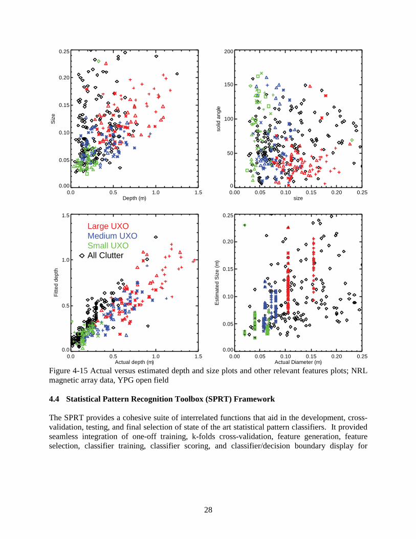
r is the distance from the object to the sensor and the magnetization tensor coordinate system must be aligned with the coordinate system of the sensor. The model parameters are found by computing the least squares (LSQ) solution between the data and the model, given a particular set of model parameters. The model parameters are found by randomly initializing a set of parameters and then applying a gradient descent algorithm to converge to a locally best-fit (minimum error) solution. The non-linear solution space creates the possibility for many locally minimum error solutions that may not be globally the best-fit to the data. To overcome this problem, the input parameter space is randomly sampled hundreds of thousands of times to find a set of good starting points for the gradient descent algorithm. Since a good initial starting point is the key to finding the best overall solution, it is important to sample the parameter space as densely as possible. The suitability of the initialization is determined by finding the error between the model and the data. This process is typically fast compared to finding the complete gradient descent solution. Once the best initial starting points are found, the full gradient descent solution can be computed for only the best N initial parameters. 4.3.7 Magnetic Model The theoretical model used is a magnetic dipole. The magnetic field anomaly due to a ferrous object can be expanded in a multi-pole expansion with the leading term representing the dipole contribution. The higher order terms fall off more sharply with distance so if the object is compact and sufficiently far from the sensor the dipole term will dominate. Target location, depth, and magnetic dipole moment (which is related to size) can be estimated from magnetometer survey data. Figure 4-15 presents estimated versus actual depth and size measures as well as plots of some relevant features.

28

Figure 4-15 Actual versus estimated depth and size plots and other relevant features plots; NRL magnetic array data, YPG open field 4.4 Statistical Pattern Recognition Toolbox (SPRT) Framework The SPRT provides a cohesive suite of interrelated functions that aid in the development, cross-validation, testing, and final selection of state of the art statistical pattern classifiers. It provided seamless integration of one-off training, k-folds cross-validation, feature generation, feature selection, classifier training, classifier scoring, and classifier/decision boundary display for

0.0 0.5 1.0 1.5Depth (m)

0.00

0.05

0.10

0.15

0.20

0.25S

ize

0.00 0.05 0.10 0.15 0.20 0.25size

0

50

100

150

200

solid

ang

le

0.0 0.5 1.0 1.5Actual depth (m)

0.0

0.5

1.0

1.5

Fitte

d de

pth

0.00 0.05 0.10 0.15 0.20 0.25Actual Diameter (m)

0.00

0.05

0.10

0.15

0.20

0.25E

stim

ated

Siz

e (m

)


29

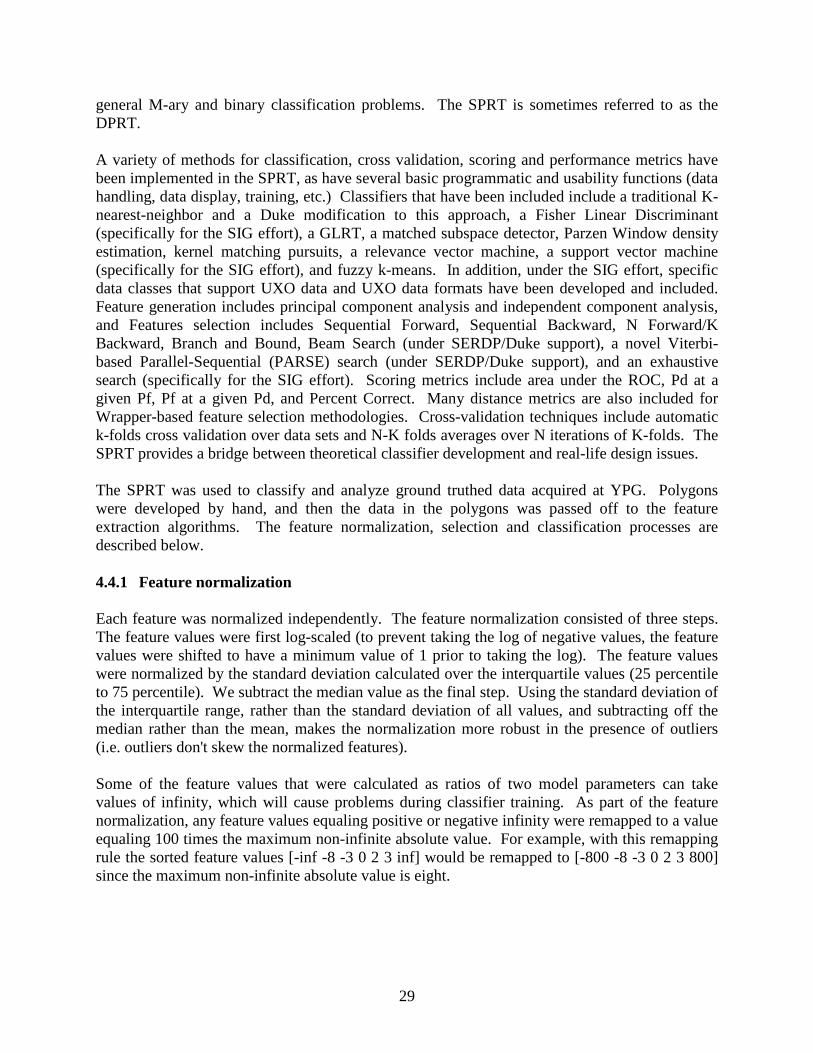
general M-ary and binary classification problems. The SPRT is sometimes referred to as the DPRT. A variety of methods for classification, cross validation, scoring and performance metrics have been implemented in the SPRT, as have several basic programmatic and usability functions (data handling, data display, training, etc.) Classifiers that have been included include a traditional K-nearest-neighbor and a Duke modification to this approach, a Fisher Linear Discriminant (specifically for the SIG effort), a GLRT, a matched subspace detector, Parzen Window density estimation, kernel matching pursuits, a relevance vector machine, a support vector machine (specifically for the SIG effort), and fuzzy k-means. In addition, under the SIG effort, specific data classes that support UXO data and UXO data formats have been developed and included. Feature generation includes principal component analysis and independent component analysis, and Features selection includes Sequential Forward, Sequential Backward, N Forward/K Backward, Branch and Bound, Beam Search (under SERDP/Duke support), a novel Viterbi-based Parallel-Sequential (PARSE) search (under SERDP/Duke support), and an exhaustive search (specifically for the SIG effort). Scoring metrics include area under the ROC, Pd at a given Pf, Pf at a given Pd, and Percent Correct. Many distance metrics are also included for Wrapper-based feature selection methodologies. Cross-validation techniques include automatic k-folds cross validation over data sets and N-K folds averages over N iterations of K-folds. The SPRT provides a bridge between theoretical classifier development and real-life design issues. The SPRT was used to classify and analyze ground truthed data acquired at YPG. Polygons were developed by hand, and then the data in the polygons was passed off to the feature extraction algorithms. The feature normalization, selection and classification processes are described below. 4.4.1 Feature normalization Each feature was normalized independently. The feature normalization consisted of three steps. The feature values were first log-scaled (to prevent taking the log of negative values, the feature values were shifted to have a minimum value of 1 prior to taking the log). The feature values were normalized by the standard deviation calculated over the interquartile values (25 percentile to 75 percentile). We subtract the median value as the final step. Using the standard deviation of the interquartile range, rather than the standard deviation of all values, and subtracting off the median rather than the mean, makes the normalization more robust in the presence of outliers (i.e. outliers don't skew the normalized features). Some of the feature values that were calculated as ratios of two model parameters can take values of infinity, which will cause problems during classifier training. As part of the feature normalization, any feature values equaling positive or negative infinity were remapped to a value equaling 100 times the maximum non-infinite absolute value. For example, with this remapping rule the sorted feature values [-inf -8 -3 0 2 3 inf] would be remapped to [-800 -8 -3 0 2 3 800] since the maximum non-infinite absolute value is eight.

30

4.4.2 Feature selection Feature selection was implemented using wrapper techniques, measuring classification performance on a set of training data with various sets of features to find the best-performing feature set. The feature selection technique was performed using four classifiers described below. A forward sequential feature selection routine was used to find a rank-ordered list of the 20 best features for models having more than 20 features; for models with fewer than 20 features it was possible to perform an exhaustive feature search for the best feature set containing between 1 and 5 features. The wrapper techniques used k-folds cross-validation with k = 5. The fitness metric for each feature set or feature, used to determine the best feature set in the exhaustive search or which feature to add next in the forward sequential search, was the area under the ROC curve. If two feature sets / features have the same area under the ROC curve, the probability of false alarm at a probability of detection equaling 90% was used as a tie-breaker. The number of features was selected to maximize the fitness metric (area under the ROC curve) on the training data. 4.4.3 Classifiers K-NN: The k-nearest neighbor (K-NN) classification rule uses the k neighbors of an unlabeled test point to estimate its label. The posterior probability of the class H given the unlabeled test point x, p(H|x), is approximated by the proportion of the k neighbors in the labeled training data that are from class H. Thus, K-NN provides a simple and intuitive classification rule where new data points are labeled according to a majority-vote of the nearest neighbors. K-NN has been shown to have attractive asymptotic properties when the amount of available training data and the number of neighbors k are both large. GLRT: The generalized likelihood ratio test is grounded in Bayesian decision theory. The likelihood ratio test λ(x) is defined at the ratio of two conditional probabilities: the probability of the features given H1 p(x|H1) and the probability of the features given H0 p(x|H0), where H1 and H0 correspond to the UXO and clutter classes, respectively. Given probability distributions of the feature values for the classes of UXO and clutter, the likelihood ratio test can be calculated for any new data point by taking the ratio of the likelihoods of the features of the new data point under both H1 and H0. However, one issue arising with the likelihood ratio test is that the probability distributions p(x|H1) and p(x|H0) are rarely known. Thus, one solution is to assume the conditional probability distributions follow a parametric form with parameters estimated using the training data. The GLRT is calculated using the conditional probabilities that are dependent on the estimated parameters [8]. In our implementation it is assumed that the UXO features have a Gaussian distribution. The clutter features were modeled using an improper uniform distribution that does not have estimated parameters; therefore, we are not training our clutter class (which can be very diverse and difficult to estimate). SVM and RVM: The support vector machine (SVM) and relevance vector machine (RVM) are generalized linear classifiers. In both the SVM and RVM, the use of a kernel to represent the input data introduces nonlinearity and can transform the data into a higher dimensional space

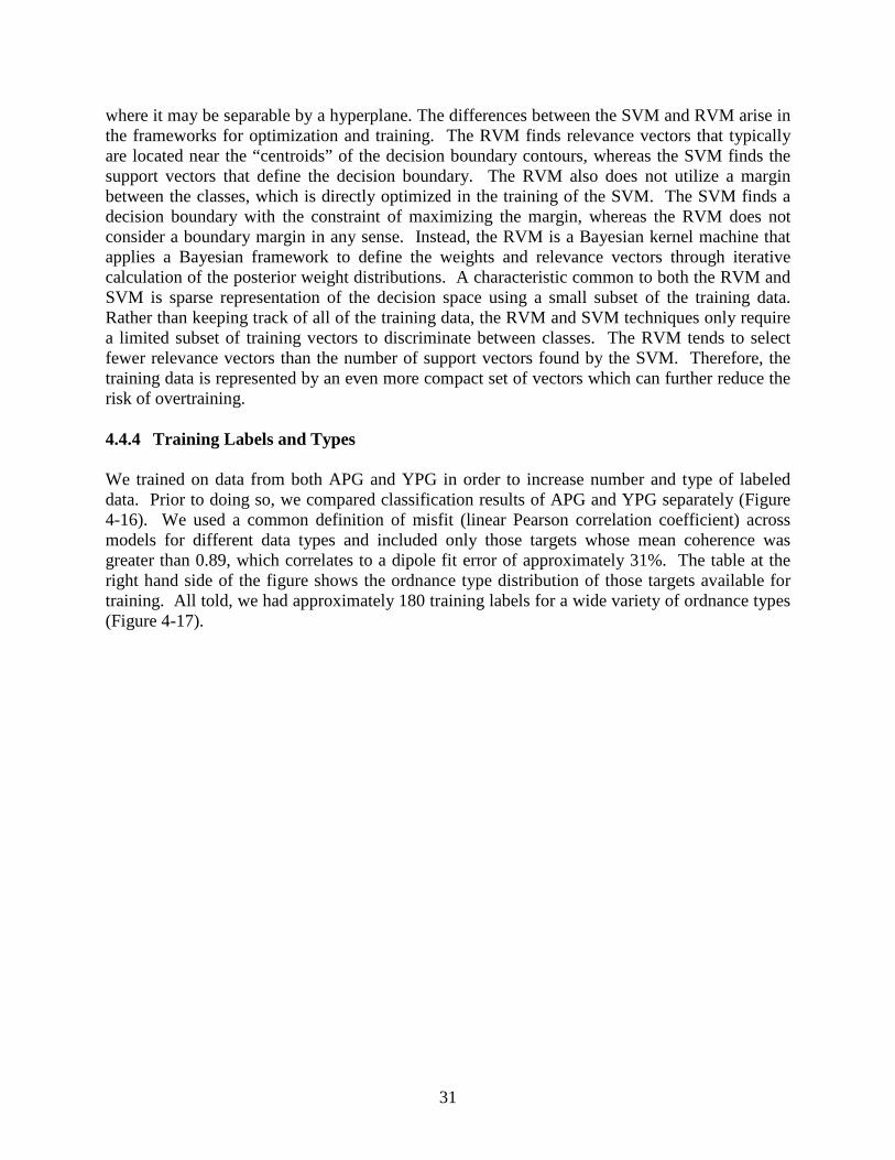
31

where it may be separable by a hyperplane. The differences between the SVM and RVM arise in the frameworks for optimization and training. The RVM finds relevance vectors that typically are located near the “centroids” of the decision boundary contours, whereas the SVM finds the support vectors that define the decision boundary. The RVM also does not utilize a margin between the classes, which is directly optimized in the training of the SVM. The SVM finds a decision boundary with the constraint of maximizing the margin, whereas the RVM does not consider a boundary margin in any sense. Instead, the RVM is a Bayesian kernel machine that applies a Bayesian framework to define the weights and relevance vectors through iterative calculation of the posterior weight distributions. A characteristic common to both the RVM and SVM is sparse representation of the decision space using a small subset of the training data. Rather than keeping track of all of the training data, the RVM and SVM techniques only require a limited subset of training vectors to discriminate between classes. The RVM tends to select fewer relevance vectors than the number of support vectors found by the SVM. Therefore, the training data is represented by an even more compact set of vectors which can further reduce the risk of overtraining. 4.4.4 Training Labels and Types We trained on data from both APG and YPG in order to increase number and type of labeled data. Prior to doing so, we compared classification results of APG and YPG separately (Figure 4-16). We used a common definition of misfit (linear Pearson correlation coefficient) across models for different data types and included only those targets whose mean coherence was greater than 0.89, which correlates to a dipole fit error of approximately 31%. The table at the right hand side of the figure shows the ordnance type distribution of those targets available for training. All told, we had approximately 180 training labels for a wide variety of ordnance types (Figure 4-17).

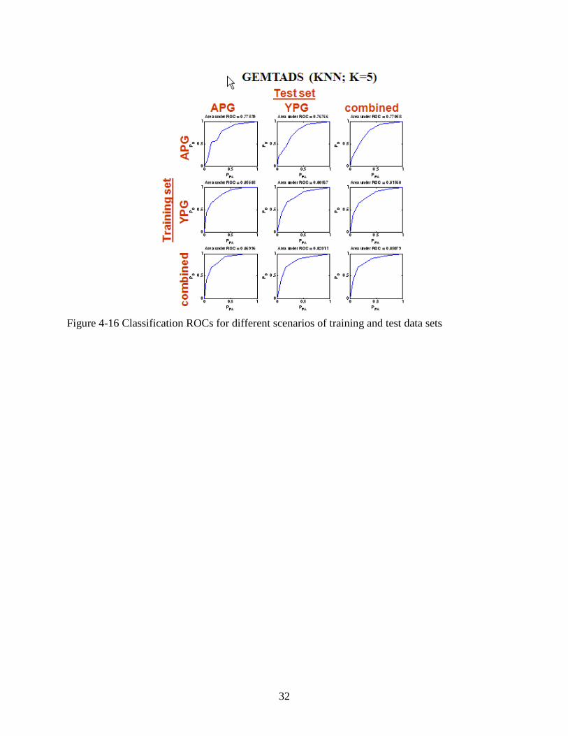
32

Figure 4-16 Classification ROCs for different scenarios of training and test data sets

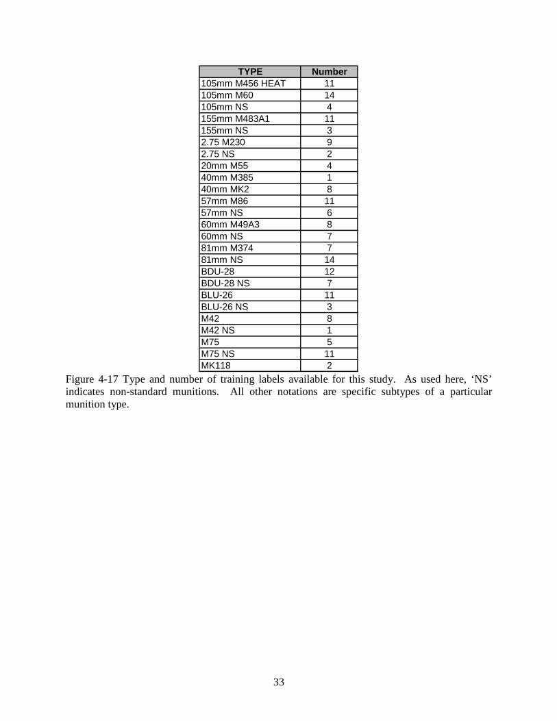
33

Figure 4-17 Type and number of training labels available for this study. As used here, ‘NS’ indicates non-standard munitions. All other notations are specific subtypes of a particular munition type.

TYPE Number105mm M456 HEAT 11105mm M60 14105mm NS 4155mm M483A1 11155mm NS 32.75 M230 92.75 NS 220mm M55 440mm M385 140mm MK2 857mm M86 1157mm NS 660mm M49A3 860mm NS 781mm M374 781mm NS 14BDU-28 12BDU-28 NS 7BLU-26 11BLU-26 NS 3M42 8M42 NS 1M75 5M75 NS 11MK118 2

34

5. Results and Discussion To compare classification performances, we first performed a forward sequential feature selection to identify which features produced the best performance for each combination of data type and model (Figure 5-1). We started with features that are intrinsic to the target (i.e., principal axis polarizability, moments, characteristic frequencies, etc.), then generated candidate subsets by adding a single feature to the set of previously-selected features, and finally evaluated subsets using a KNN classifier. Performance measures were defined to be (i) the area under (AUC) the ROC curve and (ii) the probability of false alarm (PFA) at a probability of detection (Pd) of 0.95. Example ROC curves for specific, but arbitrary AUC measures, are shown Figure 5-2. The full results of the feature selection and performance evaluation are presented in detail in the Appendix. In the following sections, we high light and discuss the most salient results.

Figure 5-1 Schematic showing the forward sequential feature selection process adopted for identifying the best performing set of features for each combination of data type and model.

Figure 5-2 Comparison of hypothetical ROC curves possessing specific AUC measures

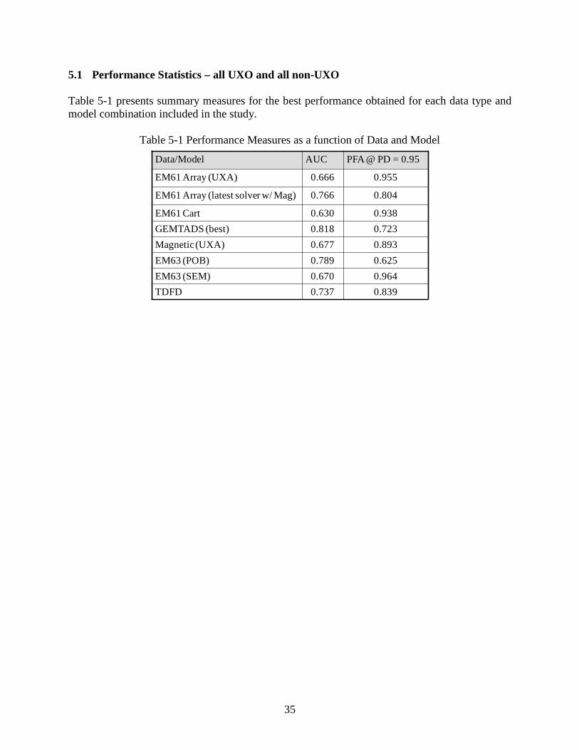
35

5.1 Performance Statistics – all UXO and all non-UXO Table 5-1 presents summary measures for the best performance obtained for each data type and model combination included in the study.

Table 5-1 Performance Measures as a function of Data and Model

Data/Model AUC PFA @ PD = 0.95

EM61 Array (UXA) 0.666 0.955

EM61 Array (latest solver w/ Mag) 0.766 0.804

EM61 Cart 0.630 0.938GEMTADS (best) 0.818 0.723Magnetic (UXA) 0.677 0.893EM63 (POB) 0.789 0.625EM63 (SEM) 0.670 0.964TDFD 0.737 0.839

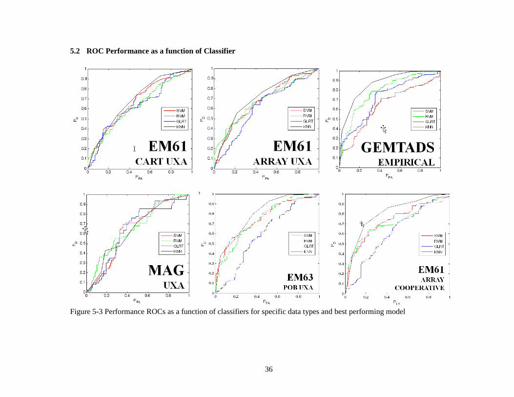
36

5.2 ROC Performance as a function of Classifier

Figure 5-3 Performance ROCs as a function of classifiers for specific data types and best performing model

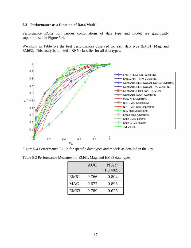
37

5.3 Performance as a function of Data/Model Performance ROCs for various combinations of data type and model are graphically superimposed in Figure 5-4. We show in Table 5-2 the best performances observed for each data type (EM61, Mag, and EM63). This analysis utilized a KNN classifier for all data types.

Figure 5-4 Performance ROCs for specific data types and models as detailed in the key. Table 5-2 Performance Measures for EM61, Mag, and EM63 data types

0 0.2 0.4 0.6 0.8 10

0.1

0.2

0.3

0.4

0.5

0.6

0.7

0.8

0.9

1

PFA

PD

EM61ARRAY NRL COMBINEEM61CART TTFW COMBINEGEMTADS ELLIPSOIDAL SCALE COMBINEGEMTADS ELLIPSOIDAL TAU COMBINEGEMTADS EMPIRICAL COMBINEGEMTADS LOOP COMBINEMAG NRL COMBINENRL EM61 CooperativeNRL EM61 NonCooperativeNRL Mag CooperativeEM63 WES COMBINECarin EM63 paramsCarin GEM3 paramsTDFD FITS

AUC PFA @ PD=0.95

EM61 0.766 0.804

MAG 0.677 0.893

EM63 0.789 0.625

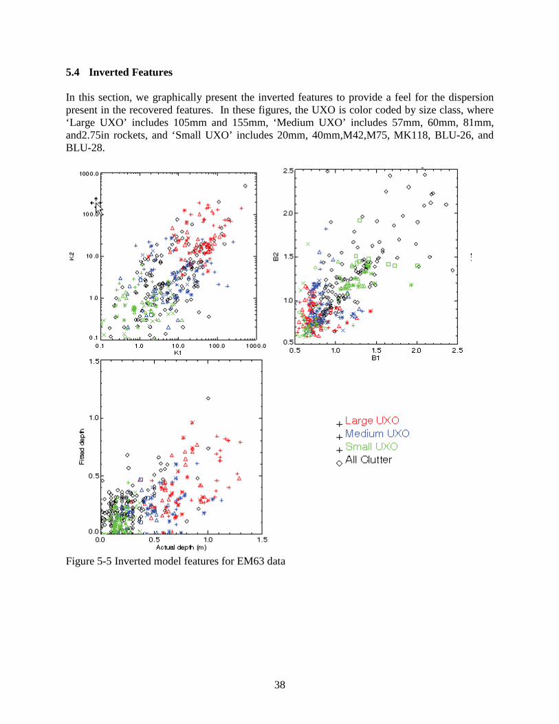
38

5.4 Inverted Features In this section, we graphically present the inverted features to provide a feel for the dispersion present in the recovered features. In these figures, the UXO is color coded by size class, where ‘Large UXO’ includes 105mm and 155mm, ‘Medium UXO’ includes 57mm, 60mm, 81mm, and2.75in rockets, and ‘Small UXO’ includes 20mm, 40mm,M42,M75, MK118, BLU-26, and BLU-28.

Figure 5-5 Inverted model features for EM63 data

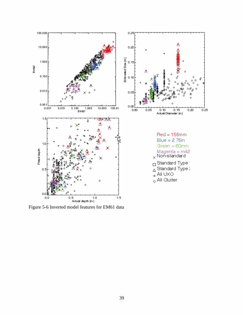
39

Figure 5-6 Inverted model features for EM61 data

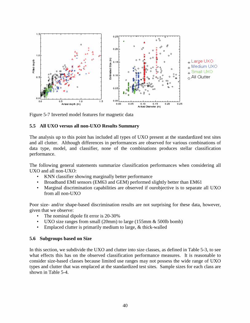
40

Figure 5-7 Inverted model features for magnetic data 5.5 All UXO versus all non-UXO Results Summary The analysis up to this point has included all types of UXO present at the standardized test sites and all clutter. Although differences in performances are observed for various combinations of data type, model, and classifier, none of the combinations produces stellar classification performance. The following general statements summarize classification performances when considering all UXO and all non-UXO:

• KNN classifier showing marginally better performance • Broadband EMI sensors (EM63 and GEM) performed slightly better than EM61 • Marginal discrimination capabilities are observed if ourobjective is to separate all UXO

from all non-UXO Poor size- and/or shape-based discrimination results are not surprising for these data, however, given that we observe:

• The nominal dipole fit error is 20-30% • UXO size ranges from small (20mm) to large (155mm & 500lb bomb) • Emplaced clutter is primarily medium to large, & thick-walled

5.6 Subgroups based on Size In this section, we subdivide the UXO and clutter into size classes, as defined in Table 5-3, to see what effects this has on the observed classification performance measures. It is reasonable to consider size-based classes because limited use ranges may not possess the wide range of UXO types and clutter that was emplaced at the standardized test sites. Sample sizes for each class are shown in Table 5-4.

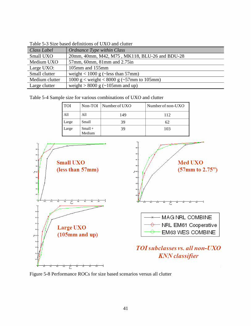
41

Table 5-3 Size based definitions of UXO and clutter Class Label Ordnance Type within Class Small UXO 20mm, 40mm, M42, M75 , MK118, BLU-26 and BDU-28 Medium UXO 57mm, 60mm, 81mm and 2.75in Large UXO: 105mm and 155mm Small clutter weight < 1000 g (~less than 57mm) Medium clutter 1000 g < weight < 8000 g (~57mm to 105mm) Large clutter weight > 8000 g (~105mm and up) Table 5-4 Sample size for various combinations of UXO and clutter

Figure 5-8 Performance ROCs for size based scenarios versus all clutter

TOI Non-TOI Number of UXO Number of non-UXO

All All 149 112Large Small 39 62Large Small +

Medium39 103

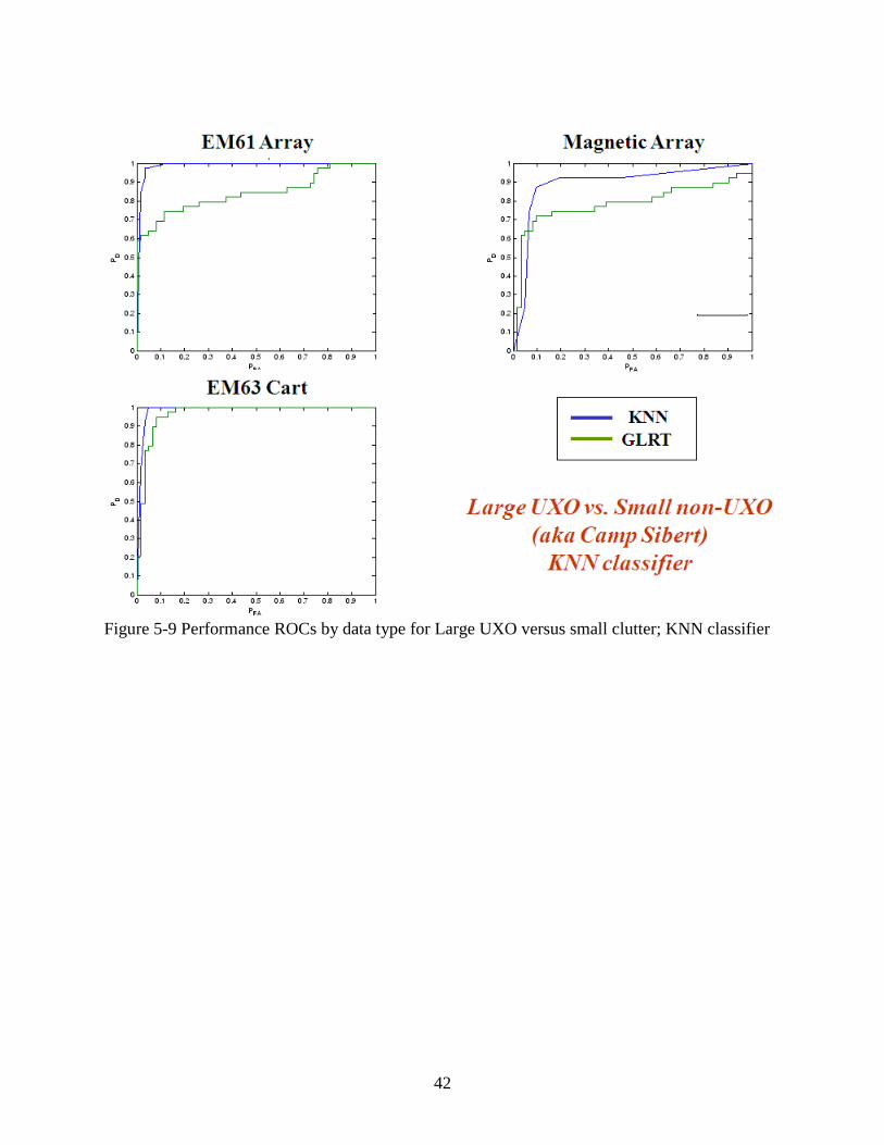
42

Figure 5-9 Performance ROCs by data type for Large UXO versus small clutter; KNN classifier

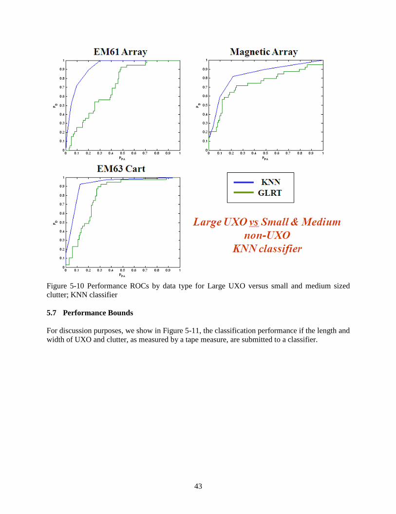
43

Figure 5-10 Performance ROCs by data type for Large UXO versus small and medium sized clutter; KNN classifier 5.7 Performance Bounds For discussion purposes, we show in Figure 5-11, the classification performance if the length and width of UXO and clutter, as measured by a tape measure, are submitted to a classifier.

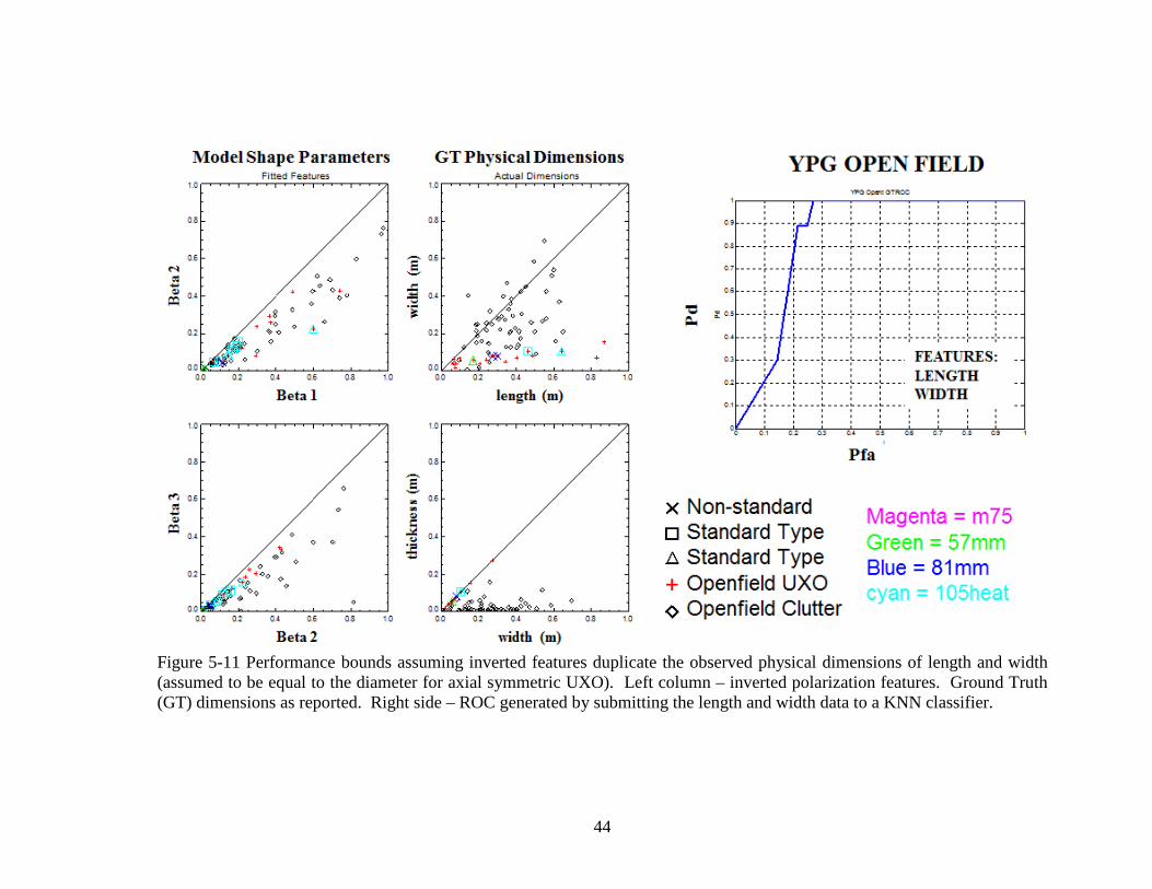
44

Figure 5-11 Performance bounds assuming inverted features duplicate the observed physical dimensions of length and width (assumed to be equal to the diameter for axial symmetric UXO). Left column – inverted polarization features. Ground Truth (GT) dimensions as reported. Right side – ROC generated by submitting the length and width data to a KNN classifier.

45

5.8 Comparison of Dynamic versus Static Data Collection In this section, we present a comparison between data collected in cued mode at APG with reconnaissance data collected in dynamic modes. The cued data collection was acquired, in support of this effort, to provide an opportunity for removing data problems associated with imprecise spatial registrations. For cued data collection, we acquired EM61 data using a mobile template as shown in Figure 5-12. We used an EM61 coil set of 0.5x1m coils. Data were collected on a 7x5 point rectangle (25cm x 50cm), covering an area of 1.25 x 2.0m. The bottom coil was 20cm above the ground.

Figure 5-12 Photographs of three different collection schemes compared in this section. Top left shows a cued deployment using a fixed sampling scheme. Top right shows the TEMTADS vehicular array. Bottom left shows a man-towed deployment scheme. Figure 5-13 plots the recovered dipole fit errors versus SNR for common anomalies but different collection schemes. It is evident from this figure, and from Table 5-5, that the template (cued) data possess smaller fit errors than dynamic survey data and that fit error is inversely related to SNR.

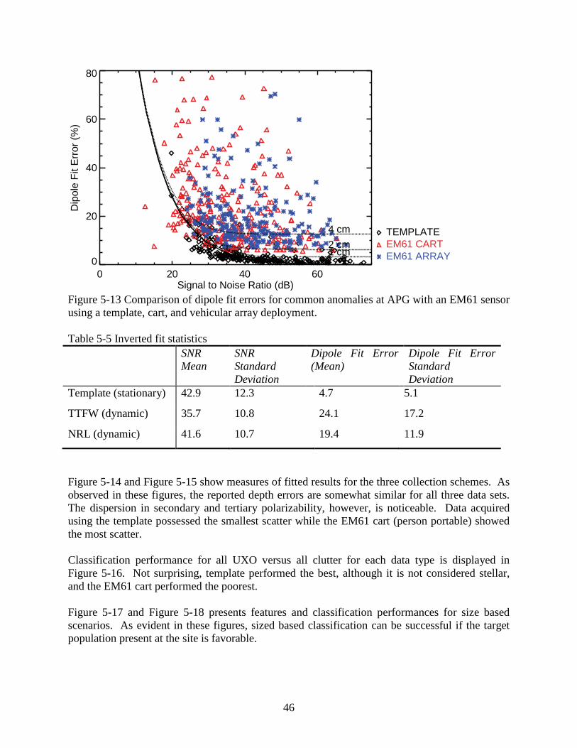
46

Figure 5-13 Comparison of dipole fit errors for common anomalies at APG with an EM61 sensor using a template, cart, and vehicular array deployment. Table 5-5 Inverted fit statistics SNR

Mean SNR Standard Deviation

Dipole Fit Error (Mean)

Dipole Fit Error Standard Deviation

Template (stationary) 42.9 12.3 4.7 5.1

TTFW (dynamic) 35.7 10.8 24.1 17.2

NRL (dynamic) 41.6 10.7 19.4 11.9

Figure 5-14 and Figure 5-15 show measures of fitted results for the three collection schemes. As observed in these figures, the reported depth errors are somewhat similar for all three data sets. The dispersion in secondary and tertiary polarizability, however, is noticeable. Data acquired using the template possessed the smallest scatter while the EM61 cart (person portable) showed the most scatter. Classification performance for all UXO versus all clutter for each data type is displayed in Figure 5-16. Not surprising, template performed the best, although it is not considered stellar, and the EM61 cart performed the poorest. Figure 5-17 and Figure 5-18 presents features and classification performances for size based scenarios. As evident in these figures, sized based classification can be successful if the target population present at the site is favorable.

0 20 40 60Signal to Noise Ratio (dB)

0

20

40

60

80D

ipol

e Fi

t Err

or (%

)

TEMPLATEEM61 CARTEM61 ARRAY1 cm

2 cm4 cm

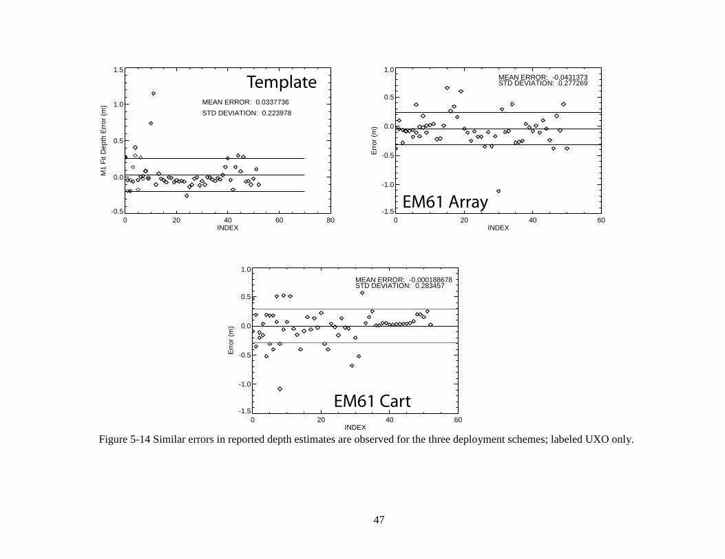
47

Figure 5-14 Similar errors in reported depth estimates are observed for the three deployment schemes; labeled UXO only.

0 20 40 60 80INDEX

-0.5

0.0

0.5

1.0

1.5

M1

Fit D

epth

Err

or (m

) MEAN ERROR: 0.0337736STD DEVIATION: 0.223978

Template

0 20 40 60INDEX

-1.5

-1.0

-0.5

0.0

0.5

1.0

Erro

r (m

)

MEAN ERROR: -0.0431373STD DEVIATION: 0.277269

EM61 Array

0 20 40 60INDEX

-1.5

-1.0

-0.5

0.0

0.5

1.0

Erro

r (m

)

MEAN ERROR: -0.000188678STD DEVIATION: 0.283457

EM61 Cart

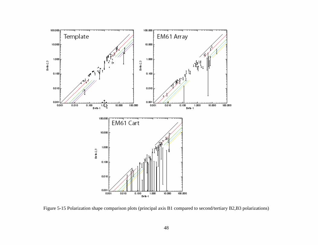
48

Figure 5-15 Polarization shape comparison plots (principal axis B1 compared to second/tertiary B2,B3 polarizations)

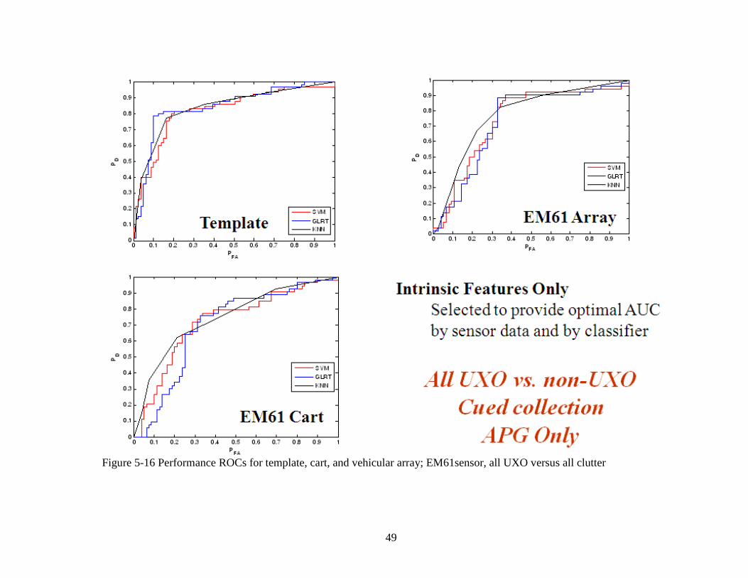
49

Figure 5-16 Performance ROCs for template, cart, and vehicular array; EM61sensor, all UXO versus all clutter

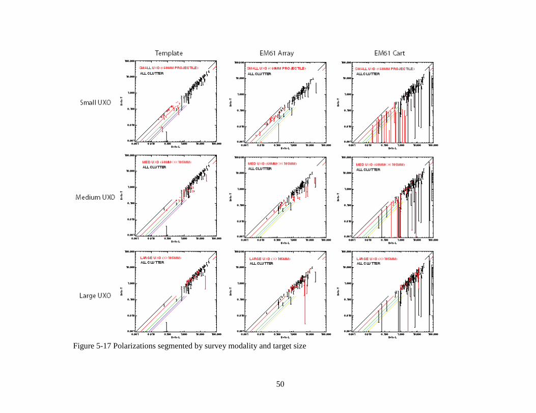
50

Figure 5-17 Polarizations segmented by survey modality and target size

Templat e EM61 Array EM61 Cart ~- ~0- ~-

Ct.t.:u. UXO•( , (J,U,I PRO.EC11t..E • / Ct.t.:L. U>O •<, OMM PROJEC11t..E • .4LLCWTn:R .4LLCWTT1R .4LLCWT'Il:R ·- ·- J(l ·-

·- ·- ·-Smaii UXO ! ' # ' • f • 0.~ 0.~ 0.~

... ... ... ~· /

OM' h

OM' OM' ·- ~- ; ..... ... ·- ·-"''"·I. ~-

t.IEOUX0 •401,ti< X<100t.IM• _(-~0- ~-

t.IEO UXO •<Ot,t,t<X<lOOt.IM• ~ t.IEO J XO •' OI.U,I( >*: lO;t,u,t• ·- .4LLCWT'TliiR ~~\ .4LLCWTT1R .4LLCWT'n:R ·- #!(~ ·-f l[ ·- .' ,, ·- ·-Medium UXO ! ' ,~.I ' r • • 0~ 0~ . r 0.~

... ~ ... /~

... OM' OM' OM' ~.

OM' ... 0.~ ·- ·- ~- OM' ... 0.~ ·- ·- ~- o•• •O» 0.~ ·- ·- ~-..... ~. ..... .. ... ~-

/ ~0- ~-

URGE UXO OOl•>t.U,I • LARGE U>:) • >O l o;t,t/,1 • UIHE UXO 00 100t.U,I • .4LLCWT'Il:R .4LLCWT1&'; .4lLCWT'niiR ·- ~~ ·- (t ·-

·- 'l I ·- :;; ·-' ' ' Large UXO • r • • 0~ 0.~ 0.~

... ~ ... ... p ~~ OM' OM' OM'

OM' ... 0.~ ·- ·- ~- OM' ... 0.~ ·- ·- ~- o•• •O» 0.~ ·- ·- ~-..... ~. ..... ~. ..... ~.

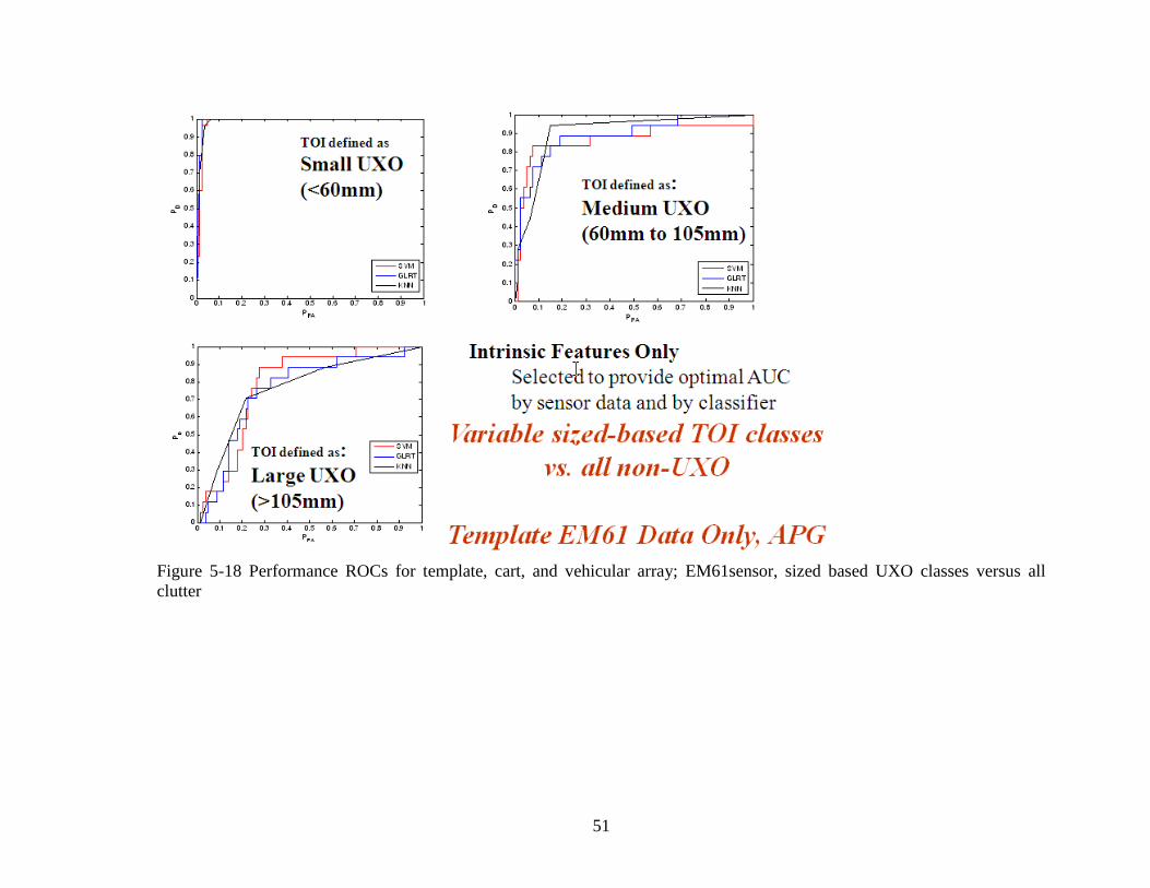
51

Figure 5-18 Performance ROCs for template, cart, and vehicular array; EM61sensor, sized based UXO classes versus all clutter

52

5.9 Discussion Our objective was to study discrimination capabilities of feature based characterization and classification techniques using data of opportunity acquired by others at the UXO Standardized Test Sites in APG and YPG. The fundamental issues investigated included the model used during characterization and the impact that classifier selection has on classification performance. After re-leveling and lagging the EM61 cart data, we inverted anomaly data for each data type using dipole, ellipsoidal, empirical, loop fit, joint frequency-time domain, and singularity expansion models. We then classified the resulting feature vectors with SVM, RVM, GLRT, and KNN statistical classifiers. We evaluated classification performance using two metrics derived from ROC curves; namely, (i) the total area under the curve and (ii) the probability of false alarms at 0.95 probability of detection. We selected five data sets to include in this study based on data quality, type, signal-to-noise, and availability at appropriate intermediate processing stages. The datasets included time-domain EM61 (man-towed single sensor cart and vehicle-towed array), time-domain EM63, frequency-domain GEM-3, and magnetic data. None of the classifiers or sensor/model combinations performed well when the TOI included 20mm through 155mm because the scatter of the features covered much of the feature space and thus overlapped with the features for clutter items. When the TOI were narrowed based on size (small, medium and large) the performance improved significantly. A related cued data collection and comparison exercise showed an improved capability with regard to deriving meaningful shape parameters when compared to data acquired on dynamic platforms.

6. Conclusions and Implications for Future Research/Implementation Our efforts to discriminate UXO from clutter using shape based information derived by inverting dynamic EM61, EM63, GEM, or magnetic data acquired at APG and YPG on dynamic platforms resulted in moderate to poor classification performances for all combinations. Classifying based on inverted size, however, should be relatively successful and may prove useful at limited-use sites that contain a small range of ordnance types. The degree of success will depend entirely on the inherent size differences between the UXO and clutter at a given site. The implication for future research is that new sensor technologies are required to realize acceptable classification performances. Given that there are multiple advanced sensors currently in development that are designed to maximize discrimination capabilities and mitigate limitations associated with single monostatic transmit-receive EMI systems, we recommend focusing future analyses efforts on their data.

53

Literature Cited [1] http://aec.army.mil/usaec/technology/uxo03f.html. [2] Miller, J., Bell, T., Soukup, J., and Keiswetter, D., Simple phenomenological models for

wideband frequency-domain electromagnetic induction, IEEE Transactions on Geoscience and Remote Sensing, Vol., 39, No. 6., June 2001.

[3] Barrow, B., Khadr, N., Miller, J., and Nelson, H., An empirically based ellipsoidal model for multiple frequency EMI signatures from UXO, SAGEEP, 2005.

[4] Miller, J., Quantification of UXO variability for Target Discrimination, Strategic Environmental Research and Development Program, UX-1313, August 2006.

[5] Barrowes, B., O’Neill, K., Grzegorczyk, T., Chen, X., Kong, J., 2004, Broadband analytical magnetoquasistatic electromagnetic induction solution for a conducting and permeable spheroid, IEEE Transactions on Geoscience and Remote Sensing, v. 42, no. 11, November 2004.

[6] Lawson, C. L., Hanson, R. J., Solving Least Square Problems, Prentice Hall, Englewood Cliffs, NJ. 1974.

[7] Zhang Y, Collins L, Yu H, Baum C, Carin L, 2003, Sensing of unexploded ordnance with magnetometer and induction data: theory and signal processing. IEEE Trans. Geoscience Remote Sensing v. 41: 1005–1015.

[8] McDonough R. N., Whalen A. D., Detection of Signals in Noise, Elsevier Science and Technology Books, April 1995.

[9] Beal M, Variational Algorithms for Approximate Bayesian Inference. PhD thesis, Gatsby Computational Neuroscience Unit, University College London, 2003.

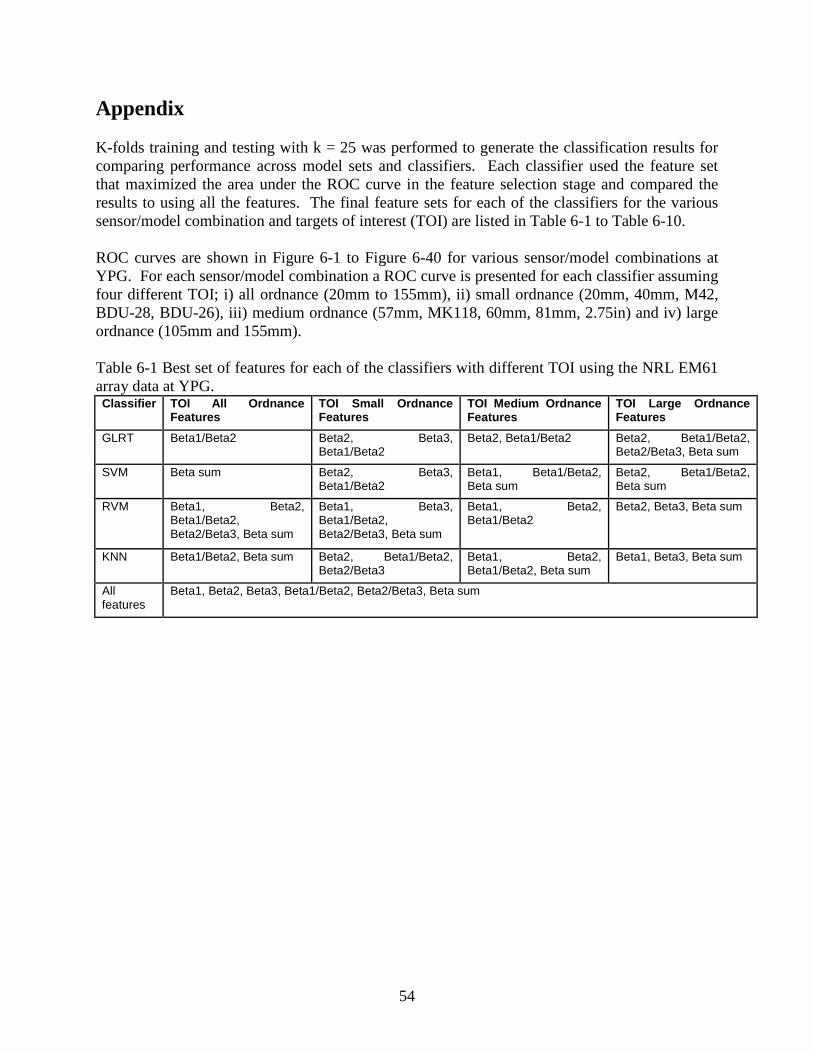
54

Appendix K-folds training and testing with k = 25 was performed to generate the classification results for comparing performance across model sets and classifiers. Each classifier used the feature set that maximized the area under the ROC curve in the feature selection stage and compared the results to using all the features. The final feature sets for each of the classifiers for the various sensor/model combination and targets of interest (TOI) are listed in Table 6-1 to Table 6-10. ROC curves are shown in Figure 6-1 to Figure 6-40 for various sensor/model combinations at YPG. For each sensor/model combination a ROC curve is presented for each classifier assuming four different TOI; i) all ordnance (20mm to 155mm), ii) small ordnance (20mm, 40mm, M42, BDU-28, BDU-26), iii) medium ordnance (57mm, MK118, 60mm, 81mm, 2.75in) and iv) large ordnance (105mm and 155mm). Table 6-1 Best set of features for each of the classifiers with different TOI using the NRL EM61 array data at YPG. Classifier TOI All Ordnance

Features TOI Small Ordnance Features

TOI Medium Ordnance Features

TOI Large Ordnance Features

GLRT Beta1/Beta2 Beta2, Beta3, Beta1/Beta2

Beta2, Beta1/Beta2 Beta2, Beta1/Beta2, Beta2/Beta3, Beta sum

SVM Beta sum Beta2, Beta3, Beta1/Beta2

Beta1, Beta1/Beta2, Beta sum

Beta2, Beta1/Beta2, Beta sum

RVM Beta1, Beta2, Beta1/Beta2, Beta2/Beta3, Beta sum

Beta1, Beta3, Beta1/Beta2, Beta2/Beta3, Beta sum

Beta1, Beta2, Beta1/Beta2

Beta2, Beta3, Beta sum

KNN Beta1/Beta2, Beta sum Beta2, Beta1/Beta2, Beta2/Beta3

Beta1, Beta2, Beta1/Beta2, Beta sum


All features

Beta1, Beta2, Beta3, Beta1/Beta2, Beta2/Beta3, Beta sum

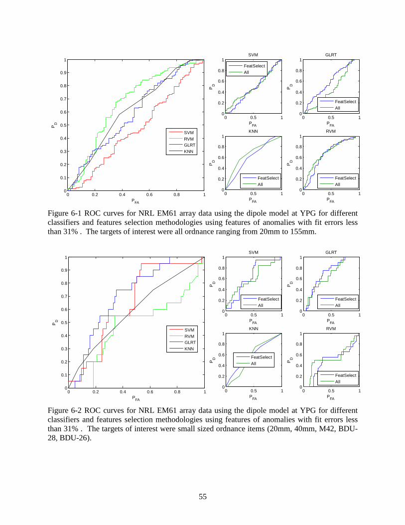
55

Figure 6-1 ROC curves for NRL EM61 array data using the dipole model at YPG for different classifiers and features selection methodologies using features of anomalies with fit errors less than 31% . The targets of interest were all ordnance ranging from 20mm to 155mm.

Figure 6-2 ROC curves for NRL EM61 array data using the dipole model at YPG for different classifiers and features selection methodologies using features of anomalies with fit errors less than 31% . The targets of interest were small sized ordnance items (20mm, 40mm, M42, BDU-28, BDU-26).

0 0.2 0.4 0.6 0.8 10

0.1

0.2

0.3

0.4

0.5

0.6

0.7

0.8

0.9

1

PFA

PD

0 0.5 10

0.2

0.4

0.6

0.8

1

PFA

PD

SVM

0 0.5 10

0.2

0.4

0.6

0.8

1

PFA

PD

GLRT

0 0.5 10

0.2

0.4

0.6

0.8

1

PFA

PD

KNN

0 0.5 10

0.2

0.4

0.6

0.8

1

PFA

PD

RVM

SVMRVMGLRTKNN

FeatSelectAll

FeatSelectAll

FeatSelectAll

FeatSelectAll

0 0.2 0.4 0.6 0.8 10

0.1

0.2

0.3

0.4

0.5

0.6

0.7

0.8

0.9

1

PFA

PD

0 0.5 10

0.2

0.4

0.6

0.8

1

PFA

PD

SVM

0 0.5 10

0.2

0.4

0.6

0.8

1

PFA

PD

GLRT

0 0.5 10

0.2

0.4

0.6

0.8

1

PFA

PD

KNN

0 0.5 10

0.2

0.4

0.6

0.8

1

PFA

PD

RVM

SVMRVMGLRTKNN

FeatSelectAll

FeatSelectAll

FeatSelectAll

FeatSelectAll

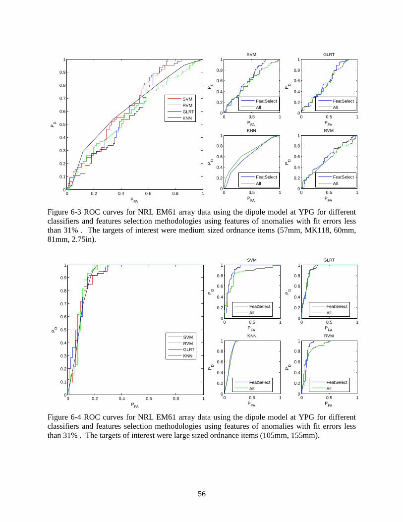
56

Figure 6-3 ROC curves for NRL EM61 array data using the dipole model at YPG for different classifiers and features selection methodologies using features of anomalies with fit errors less than 31% . The targets of interest were medium sized ordnance items (57mm, MK118, 60mm, 81mm, 2.75in).

Figure 6-4 ROC curves for NRL EM61 array data using the dipole model at YPG for different classifiers and features selection methodologies using features of anomalies with fit errors less than 31% . The targets of interest were large sized ordnance items (105mm, 155mm).

0 0.2 0.4 0.6 0.8 10

0.1

0.2

0.3

0.4

0.5

0.6

0.7

0.8

0.9

1

PFA

PD

0 0.5 10

0.2

0.4

0.6

0.8

1

PFA

PD

SVM

0 0.5 10

0.2

0.4

0.6

0.8

1

PFA

PD

GLRT

0 0.5 10

0.2

0.4

0.6

0.8

1

PFA

PD

KNN

0 0.5 10

0.2

0.4

0.6

0.8

1

PFA

PD

RVM

SVMRVMGLRTKNN

FeatSelectAll

FeatSelectAll

FeatSelectAll

FeatSelectAll

0 0.2 0.4 0.6 0.8 10

0.1

0.2

0.3

0.4

0.5

0.6

0.7

0.8

0.9

1

PFA

PD

0 0.5 10

0.2

0.4

0.6

0.8

1

PFA

PD

SVM

0 0.5 10

0.2

0.4

0.6

0.8

1

PFA

PD

GLRT

0 0.5 10

0.2

0.4

0.6

0.8

1

PFA

PD

KNN

0 0.5 10

0.2

0.4

0.6

0.8

1

PFA

PD

RVM

SVMRVMGLRTKNN

FeatSelectAll

FeatSelectAll

FeatSelectAll

FeatSelectAll

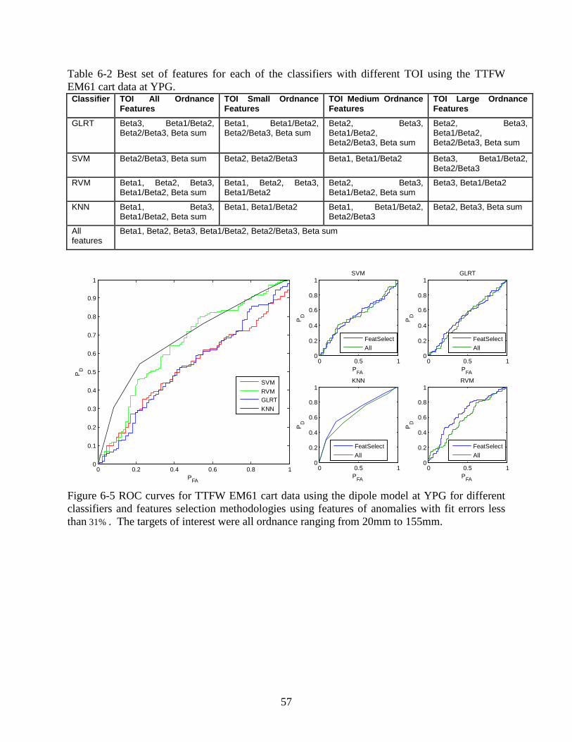
57

Table 6-2 Best set of features for each of the classifiers with different TOI using the TTFW EM61 cart data at YPG. Classifier TOI All Ordnance




GLRT Beta3, Beta1/Beta2, Beta2/Beta3, Beta sum

Beta1, Beta1/Beta2, Beta2/Beta3, Beta sum



SVM Beta2/Beta3, Beta sum Beta2, Beta2/Beta3 Beta1, Beta1/Beta2 Beta3, Beta1/Beta2, Beta2/Beta3

RVM Beta1, Beta2, Beta3, Beta1/Beta2, Beta sum

Beta1, Beta2, Beta3, Beta1/Beta2

Beta2, Beta3, Beta1/Beta2, Beta sum

Beta3, Beta1/Beta2

KNN Beta1, Beta3, Beta1/Beta2, Beta sum

Beta1, Beta1/Beta2 Beta1, Beta1/Beta2, Beta2/Beta3


All features

Beta1, Beta2, Beta3, Beta1/Beta2, Beta2/Beta3, Beta sum

Figure 6-5 ROC curves for TTFW EM61 cart data using the dipole model at YPG for different classifiers and features selection methodologies using features of anomalies with fit errors less than 31% . The targets of interest were all ordnance ranging from 20mm to 155mm.

0 0.2 0.4 0.6 0.8 10

0.1

0.2

0.3

0.4

0.5

0.6

0.7

0.8

0.9

1

PFA

PD

0 0.5 10

0.2

0.4

0.6

0.8

1

PFA

PD

SVM

0 0.5 10

0.2

0.4

0.6

0.8

1

PFA

PD

GLRT

0 0.5 10

0.2

0.4

0.6

0.8

1

PFA

PD

KNN

0 0.5 10

0.2

0.4

0.6

0.8

1

PFA

PD

RVM

SVMRVMGLRTKNN

FeatSelectAll

FeatSelectAll

FeatSelectAll

FeatSelectAll

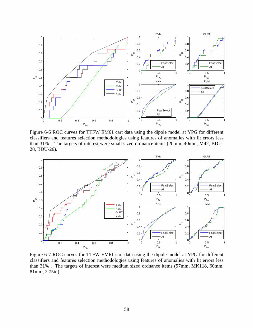
58

Figure 6-6 ROC curves for TTFW EM61 cart data using the dipole model at YPG for different classifiers and features selection methodologies using features of anomalies with fit errors less than 31% . The targets of interest were small sized ordnance items (20mm, 40mm, M42, BDU-28, BDU-26).

Figure 6-7 ROC curves for TTFW EM61 cart data using the dipole model at YPG for different classifiers and features selection methodologies using features of anomalies with fit errors less than 31% . The targets of interest were medium sized ordnance items (57mm, MK118, 60mm, 81mm, 2.75in).

0 0.2 0.4 0.6 0.8 10

0.1

0.2

0.3

0.4

0.5

0.6

0.7

0.8

0.9

1

PFA

PD

0 0.5 10

0.2

0.4

0.6

0.8

1

PFA

PD

SVM

0 0.5 10

0.2

0.4

0.6

0.8

1

PFA

PD

GLRT

0 0.5 10

0.2

0.4

0.6

0.8

1

PFA

PD

KNN

0 0.5 10

0.2

0.4

0.6

0.8

1

PFA

PD

RVM

SVMRVMGLRTKNN

FeatSelectAll

FeatSelectAll

FeatSelectAll

FeatSelectAll

0 0.2 0.4 0.6 0.8 10

0.1

0.2

0.3

0.4

0.5

0.6

0.7

0.8

0.9

1

PFA

PD

0 0.5 10

0.2

0.4

0.6

0.8

1

PFA

PD

SVM

0 0.5 10

0.2

0.4

0.6

0.8

1

PFA

PD

GLRT

0 0.5 10

0.2

0.4

0.6

0.8

1

PFA

PD

KNN

0 0.5 10

0.2

0.4

0.6

0.8

1

PFA

PD

RVM

SVMRVMGLRTKNN

FeatSelectAll

FeatSelectAll

FeatSelectAll

FeatSelectAll

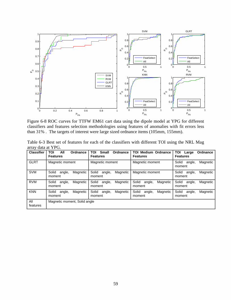
59

Figure 6-8 ROC curves for TTFW EM61 cart data using the dipole model at YPG for different classifiers and features selection methodologies using features of anomalies with fit errors less than 31% . The targets of interest were large sized ordnance items (105mm, 155mm). Table 6-3 Best set of features for each of the classifiers with different TOI using the NRL Mag array data at YPG. Classifier TOI All Ordnance




GLRT Magnetic moment Magnetic moment Magnetic moment Solid angle, Magnetic moment

SVM Solid angle, Magnetic moment

Solid angle, Magnetic moment

Magnetic moment Solid angle, Magnetic moment

RVM Solid angle, Magnetic moment




KNN Solid angle, Magnetic moment




All features

Magnetic moment, Solid angle

0 0.2 0.4 0.6 0.8 10

0.1

0.2

0.3

0.4

0.5

0.6

0.7

0.8

0.9

1

PFA

PD

0 0.5 10

0.2

0.4

0.6

0.8

1

PFA

PD

SVM

0 0.5 10

0.2

0.4

0.6

0.8

1

PFA

PD

GLRT

0 0.5 10

0.2

0.4

0.6

0.8

1

PFA

PD

KNN

0 0.5 10

0.2

0.4

0.6

0.8

1

PFA

PD

RVM

SVMRVMGLRTKNN

FeatSelectAll

FeatSelectAll

FeatSelectAll

FeatSelectAll

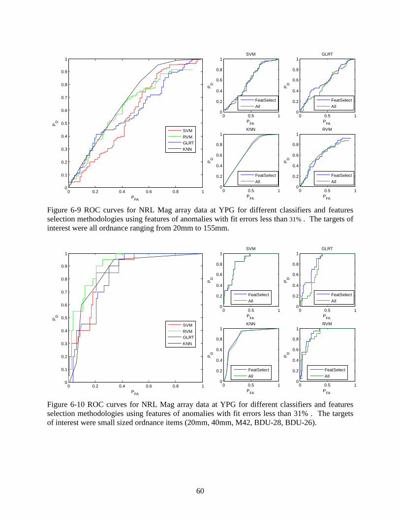
60

Figure 6-9 ROC curves for NRL Mag array data at YPG for different classifiers and features selection methodologies using features of anomalies with fit errors less than 31% . The targets of interest were all ordnance ranging from 20mm to 155mm.

Figure 6-10 ROC curves for NRL Mag array data at YPG for different classifiers and features selection methodologies using features of anomalies with fit errors less than 31% . The targets of interest were small sized ordnance items (20mm, 40mm, M42, BDU-28, BDU-26).

0 0.2 0.4 0.6 0.8 10

0.1

0.2

0.3

0.4

0.5

0.6

0.7

0.8

0.9

1

PFA

PD

0 0.5 10

0.2

0.4

0.6

0.8

1

PFA

PD

SVM

0 0.5 10

0.2

0.4

0.6

0.8

1

PFA

PD

GLRT

0 0.5 10

0.2

0.4

0.6

0.8

1

PFA

PD

KNN

0 0.5 10

0.2

0.4

0.6

0.8

1

PFA

PD

RVM

SVMRVMGLRTKNN

FeatSelectAll

FeatSelectAll

FeatSelectAll

FeatSelectAll

0 0.2 0.4 0.6 0.8 10

0.1

0.2

0.3

0.4

0.5

0.6

0.7

0.8

0.9

1

PFA

PD

0 0.5 10

0.2

0.4

0.6

0.8

1

PFA

PD

SVM

0 0.5 10

0.2

0.4

0.6

0.8

1

PFA

PD

GLRT

0 0.5 10

0.2

0.4

0.6

0.8

1

PFA

PD

KNN

0 0.5 10

0.2

0.4

0.6

0.8

1

PFA

PD

RVM

SVMRVMGLRTKNN

FeatSelectAll

FeatSelectAll

FeatSelectAll

FeatSelectAll

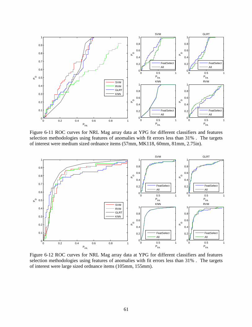
61

Figure 6-11 ROC curves for NRL Mag array data at YPG for different classifiers and features selection methodologies using features of anomalies with fit errors less than 31% . The targets of interest were medium sized ordnance items (57mm, MK118, 60mm, 81mm, 2.75in).

Figure 6-12 ROC curves for NRL Mag array data at YPG for different classifiers and features selection methodologies using features of anomalies with fit errors less than 31% . The targets of interest were large sized ordnance items (105mm, 155mm).

0 0.2 0.4 0.6 0.8 10

0.1

0.2

0.3

0.4

0.5

0.6

0.7

0.8

0.9

1

PFA

PD

0 0.5 10

0.2

0.4

0.6

0.8

1

PFA

PD

SVM

0 0.5 10

0.2

0.4

0.6

0.8

1

PFA

PD

GLRT

0 0.5 10

0.2

0.4

0.6

0.8

1

PFA

PD

KNN

0 0.5 10

0.2

0.4

0.6

0.8

1

PFA

PD

RVM

SVMRVMGLRTKNN

FeatSelectAll

FeatSelectAll

FeatSelectAll

FeatSelectAll

0 0.2 0.4 0.6 0.8 10

0.1

0.2

0.3

0.4

0.5

0.6

0.7

0.8

0.9

1

PFA

PD

0 0.5 10

0.2

0.4

0.6

0.8

1

PFA

PD

SVM

0 0.5 10

0.2

0.4

0.6

0.8

1

PFA

PD

GLRT

0 0.5 10

0.2

0.4

0.6

0.8

1

PFA

PD

KNN

0 0.5 10

0.2

0.4

0.6

0.8

1

PFA

PD

RVM

SVMRVMGLRTKNN

FeatSelectAll

FeatSelectAll

FeatSelectAll

FeatSelectAll

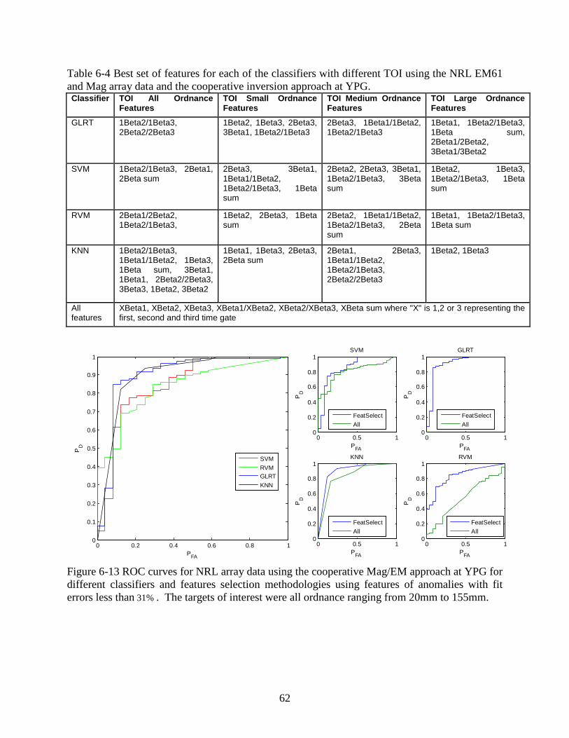
62

Table 6-4 Best set of features for each of the classifiers with different TOI using the NRL EM61 and Mag array data and the cooperative inversion approach at YPG. Classifier TOI All Ordnance




GLRT 1Beta2/1Beta3, 2Beta2/2Beta3

1Beta2, 1Beta3, 2Beta3, 3Beta1, 1Beta2/1Beta3

2Beta3, 1Beta1/1Beta2, 1Beta2/1Beta3

1Beta1, 1Beta2/1Beta3, 1Beta sum, 2Beta1/2Beta2, 3Beta1/3Beta2

SVM 1Beta2/1Beta3, 2Beta1, 2Beta sum

2Beta3, 3Beta1, 1Beta1/1Beta2, 1Beta2/1Beta3, 1Beta sum

2Beta2, 2Beta3, 3Beta1, 1Beta2/1Beta3, 3Beta sum

1Beta2, 1Beta3, 1Beta2/1Beta3, 1Beta sum

RVM 2Beta1/2Beta2, 1Beta2/1Beta3,

1Beta2, 2Beta3, 1Beta sum

2Beta2, 1Beta1/1Beta2, 1Beta2/1Beta3, 2Beta sum

1Beta1, 1Beta2/1Beta3, 1Beta sum

KNN 1Beta2/1Beta3, 1Beta1/1Beta2, 1Beta3, 1Beta sum, 3Beta1, 1Beta1, 2Beta2/2Beta3, 3Beta3, 1Beta2, 3Beta2

1Beta1, 1Beta3, 2Beta3, 2Beta sum

2Beta1, 2Beta3, 1Beta1/1Beta2, 1Beta2/1Beta3, 2Beta2/2Beta3

1Beta2, 1Beta3

All features

XBeta1, XBeta2, XBeta3, XBeta1/XBeta2, XBeta2/XBeta3, XBeta sum where "X" is 1,2 or 3 representing the first, second and third time gate

Figure 6-13 ROC curves for NRL array data using the cooperative Mag/EM approach at YPG for different classifiers and features selection methodologies using features of anomalies with fit errors less than 31% . The targets of interest were all ordnance ranging from 20mm to 155mm.

0 0.2 0.4 0.6 0.8 10

0.1

0.2

0.3

0.4

0.5

0.6

0.7

0.8

0.9

1

PFA

PD

0 0.5 10

0.2

0.4

0.6

0.8

1

PFA

PD

SVM

0 0.5 10

0.2

0.4

0.6

0.8

1

PFA

PD

GLRT

0 0.5 10

0.2

0.4

0.6

0.8

1

PFA

PD

KNN

0 0.5 10

0.2

0.4

0.6

0.8

1

PFA

PD

RVM

SVMRVMGLRTKNN

FeatSelectAll

FeatSelectAll

FeatSelectAll

FeatSelectAll

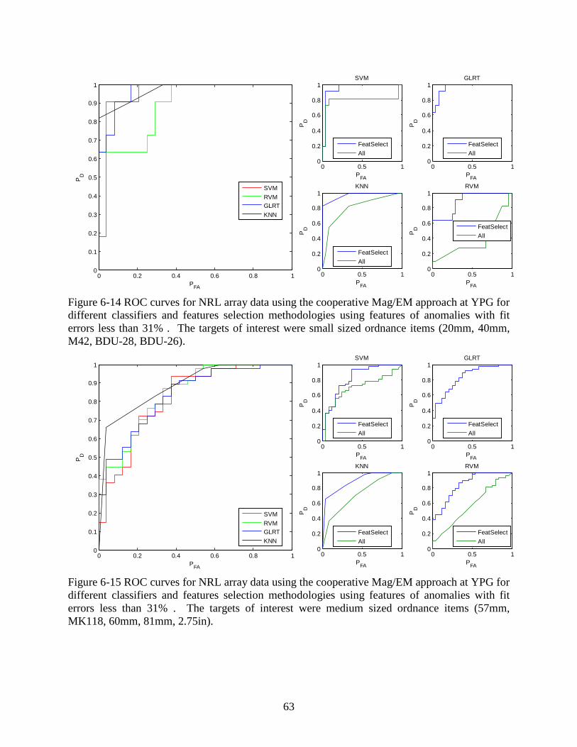
63

Figure 6-14 ROC curves for NRL array data using the cooperative Mag/EM approach at YPG for different classifiers and features selection methodologies using features of anomalies with fit errors less than 31% . The targets of interest were small sized ordnance items (20mm, 40mm, M42, BDU-28, BDU-26).

Figure 6-15 ROC curves for NRL array data using the cooperative Mag/EM approach at YPG for different classifiers and features selection methodologies using features of anomalies with fit errors less than 31% . The targets of interest were medium sized ordnance items (57mm, MK118, 60mm, 81mm, 2.75in).

0 0.2 0.4 0.6 0.8 10

0.1

0.2

0.3

0.4

0.5

0.6

0.7

0.8

0.9

1

PFA

PD

0 0.5 10

0.2

0.4

0.6

0.8

1

PFA

PD

SVM

0 0.5 10

0.2

0.4

0.6

0.8

1

PFA

PD

GLRT

0 0.5 10

0.2

0.4

0.6

0.8

1

PFA

PD

KNN

0 0.5 10

0.2

0.4

0.6

0.8

1

PFA

PD

RVM

SVMRVMGLRTKNN

FeatSelectAll

FeatSelectAll

FeatSelectAll

FeatSelectAll

0 0.2 0.4 0.6 0.8 10

0.1

0.2

0.3

0.4

0.5

0.6

0.7

0.8

0.9

1

PFA

PD

0 0.5 10

0.2

0.4

0.6

0.8

1

PFA

PD

SVM

0 0.5 10

0.2

0.4

0.6

0.8

1

PFA

PD

GLRT

0 0.5 10

0.2

0.4

0.6

0.8

1

PFA

PD

KNN

0 0.5 10

0.2

0.4

0.6

0.8

1

PFA

PD

RVM

SVMRVMGLRTKNN

FeatSelectAll

FeatSelectAll

FeatSelectAll

FeatSelectAll

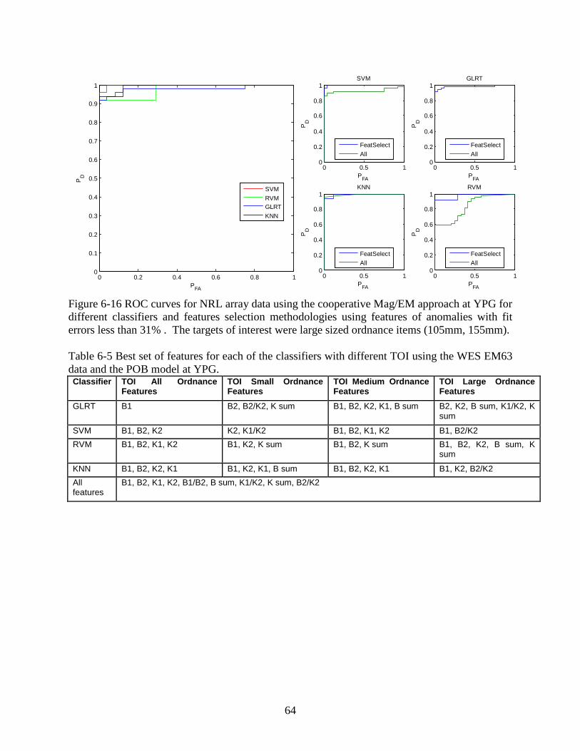
64

Figure 6-16 ROC curves for NRL array data using the cooperative Mag/EM approach at YPG for different classifiers and features selection methodologies using features of anomalies with fit errors less than 31% . The targets of interest were large sized ordnance items (105mm, 155mm). Table 6-5 Best set of features for each of the classifiers with different TOI using the WES EM63 data and the POB model at YPG. Classifier TOI All Ordnance




GLRT B1 B2, B2/K2, K sum B1, B2, K2, K1, B sum B2, K2, B sum, K1/K2, K sum

SVM B1, B2, K2 K2, K1/K2 B1, B2, K1, K2 B1, B2/K2 RVM B1, B2, K1, K2 B1, K2, K sum B1, B2, K sum B1, B2, K2, B sum, K

sum

KNN B1, B2, K2, K1 B1, K2, K1, B sum B1, B2, K2, K1 B1, K2, B2/K2 All features

B1, B2, K1, K2, B1/B2, B sum, K1/K2, K sum, B2/K2

0 0.2 0.4 0.6 0.8 10

0.1

0.2

0.3

0.4

0.5

0.6

0.7

0.8

0.9

1

PFA

PD

0 0.5 10

0.2

0.4

0.6

0.8

1

PFA

PD

SVM

0 0.5 10

0.2

0.4

0.6

0.8

1

PFA

PD

GLRT

0 0.5 10

0.2

0.4

0.6

0.8

1

PFA

PD

KNN

0 0.5 10

0.2

0.4

0.6

0.8

1

PFA

PD

RVM

SVMRVMGLRTKNN

FeatSelectAll

FeatSelectAll

FeatSelectAll

FeatSelectAll

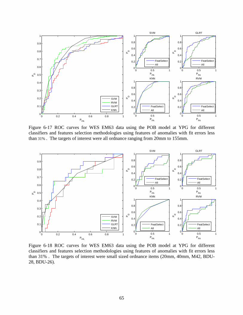
65

Figure 6-17 ROC curves for WES EM63 data using the POB model at YPG for different classifiers and features selection methodologies using features of anomalies with fit errors less than 31% . The targets of interest were all ordnance ranging from 20mm to 155mm.

Figure 6-18 ROC curves for WES EM63 data using the POB model at YPG for different classifiers and features selection methodologies using features of anomalies with fit errors less than 31% . The targets of interest were small sized ordnance items (20mm, 40mm, M42, BDU-28, BDU-26).

0 0.2 0.4 0.6 0.8 10

0.1

0.2

0.3

0.4

0.5

0.6

0.7

0.8

0.9

1

PFA

PD

0 0.5 10

0.2

0.4

0.6

0.8

1

PFA

PD

SVM

0 0.5 10

0.2

0.4

0.6

0.8

1

PFA

PD

GLRT

0 0.5 10

0.2

0.4

0.6

0.8

1

PFA

PD

KNN

0 0.5 10

0.2

0.4

0.6

0.8

1

PFA

PD

RVM

SVMRVMGLRTKNN

FeatSelectAll

FeatSelectAll

FeatSelectAll

FeatSelectAll

0 0.2 0.4 0.6 0.8 10

0.1

0.2

0.3

0.4

0.5

0.6

0.7

0.8

0.9

1

PFA

PD

0 0.5 10

0.2

0.4

0.6

0.8

1

PFA

PD

SVM

0 0.5 10

0.2

0.4

0.6

0.8

1

PFA

PD

GLRT

0 0.5 10

0.2

0.4

0.6

0.8

1

PFA

PD

KNN

0 0.5 10

0.2

0.4

0.6

0.8

1

PFA

PD

RVM

SVMRVMGLRTKNN

FeatSelectAll

FeatSelectAll

FeatSelectAll

FeatSelectAll

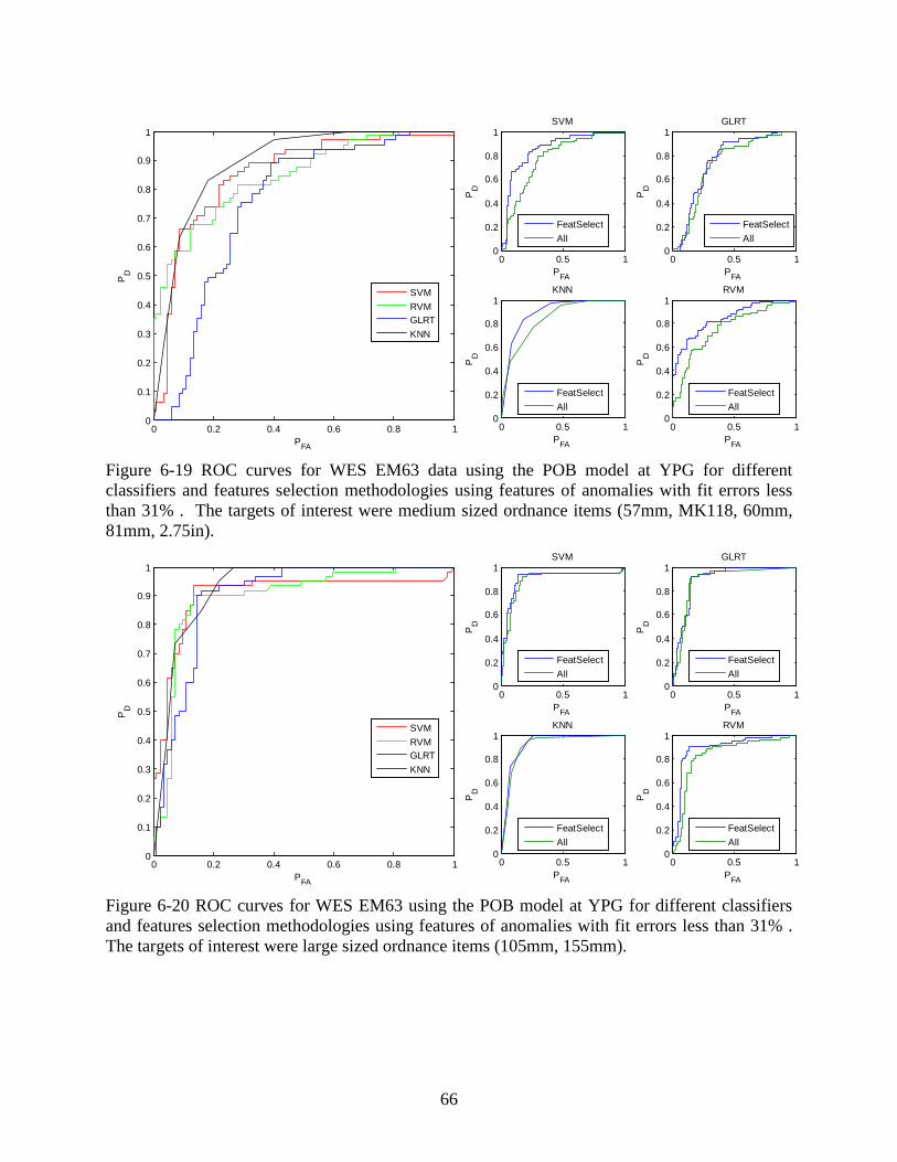
66

Figure 6-19 ROC curves for WES EM63 data using the POB model at YPG for different classifiers and features selection methodologies using features of anomalies with fit errors less than 31% . The targets of interest were medium sized ordnance items (57mm, MK118, 60mm, 81mm, 2.75in).

Figure 6-20 ROC curves for WES EM63 using the POB model at YPG for different classifiers and features selection methodologies using features of anomalies with fit errors less than 31% . The targets of interest were large sized ordnance items (105mm, 155mm).

0 0.2 0.4 0.6 0.8 10

0.1

0.2

0.3

0.4

0.5

0.6

0.7

0.8

0.9

1

PFA

PD

0 0.5 10

0.2

0.4

0.6

0.8

1

PFA

PD

SVM

0 0.5 10

0.2

0.4

0.6

0.8

1

PFA

PD

GLRT

0 0.5 10

0.2

0.4

0.6

0.8

1

PFA

PD

KNN

0 0.5 10

0.2

0.4

0.6

0.8

1

PFA

PD

RVM

SVMRVMGLRTKNN

FeatSelectAll

FeatSelectAll

FeatSelectAll

FeatSelectAll

0 0.2 0.4 0.6 0.8 10

0.1

0.2

0.3

0.4

0.5

0.6

0.7

0.8

0.9

1

PFA

PD

0 0.5 10

0.2

0.4

0.6

0.8

1

PFA

PD

SVM

0 0.5 10

0.2

0.4

0.6

0.8

1

PFA

PD

GLRT

0 0.5 10

0.2

0.4

0.6

0.8

1

PFA

PD

KNN

0 0.5 10

0.2

0.4

0.6

0.8

1

PFA

PD

RVM

SVMRVMGLRTKNN

FeatSelectAll

FeatSelectAll

FeatSelectAll

FeatSelectAll

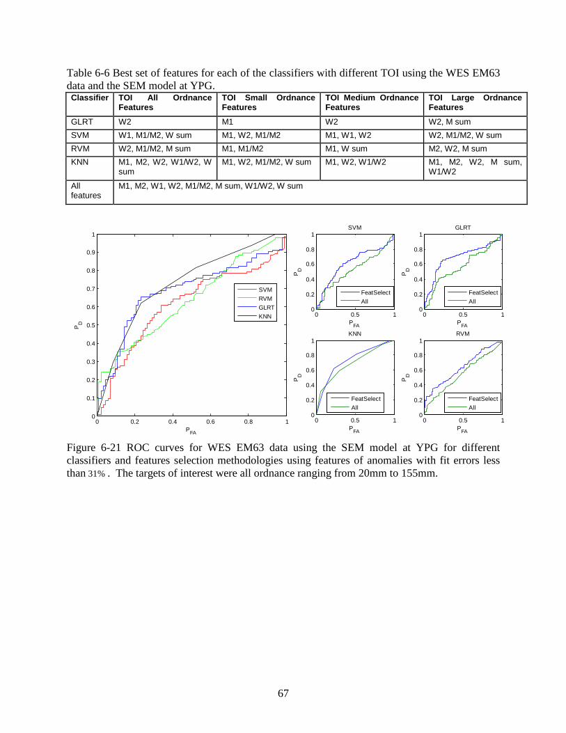
67

Table 6-6 Best set of features for each of the classifiers with different TOI using the WES EM63 data and the SEM model at YPG. Classifier TOI All Ordnance




GLRT W2 M1 W2 W2, M sum SVM W1, M1/M2, W sum M1, W2, M1/M2 M1, W1, W2 W2, M1/M2, W sum RVM W2, M1/M2, M sum M1, M1/M2 M1, W sum M2, W2, M sum KNN M1, M2, W2, W1/W2, W

sum M1, W2, M1/M2, W sum M1, W2, W1/W2 M1, M2, W2, M sum,

W1/W2

All features

M1, M2, W1, W2, M1/M2, M sum, W1/W2, W sum

Figure 6-21 ROC curves for WES EM63 data using the SEM model at YPG for different classifiers and features selection methodologies using features of anomalies with fit errors less than 31% . The targets of interest were all ordnance ranging from 20mm to 155mm.

0 0.2 0.4 0.6 0.8 10

0.1

0.2

0.3

0.4

0.5

0.6

0.7

0.8

0.9

1

PFA

PD

0 0.5 10

0.2

0.4

0.6

0.8

1

PFA

PD

SVM

0 0.5 10

0.2

0.4

0.6

0.8

1

PFA

PD

GLRT

0 0.5 10

0.2

0.4

0.6

0.8

1

PFA

PD

KNN

0 0.5 10

0.2

0.4

0.6

0.8

1

PFA

PD

RVM

SVMRVMGLRTKNN

FeatSelectAll

FeatSelectAll

FeatSelectAll

FeatSelectAll

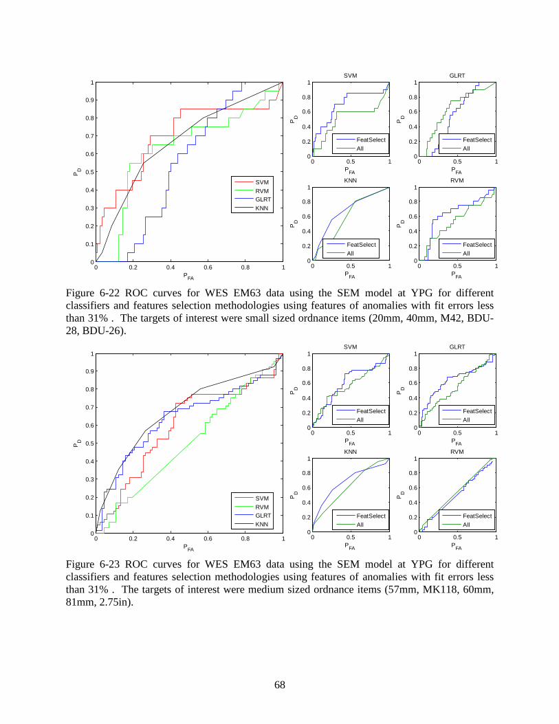
68

Figure 6-22 ROC curves for WES EM63 data using the SEM model at YPG for different classifiers and features selection methodologies using features of anomalies with fit errors less than 31% . The targets of interest were small sized ordnance items (20mm, 40mm, M42, BDU-28, BDU-26).

Figure 6-23 ROC curves for WES EM63 data using the SEM model at YPG for different classifiers and features selection methodologies using features of anomalies with fit errors less than 31% . The targets of interest were medium sized ordnance items (57mm, MK118, 60mm, 81mm, 2.75in).

0 0.2 0.4 0.6 0.8 10

0.1

0.2

0.3

0.4

0.5

0.6

0.7

0.8

0.9

1

PFA

PD

0 0.5 10

0.2

0.4

0.6

0.8

1

PFA

PD

SVM

0 0.5 10

0.2

0.4

0.6

0.8

1

PFA

PD

GLRT

0 0.5 10

0.2

0.4

0.6

0.8

1

PFA

PD

KNN

0 0.5 10

0.2

0.4

0.6

0.8

1

PFA

PD

RVM

SVMRVMGLRTKNN

FeatSelectAll

FeatSelectAll

FeatSelectAll

FeatSelectAll

0 0.2 0.4 0.6 0.8 10

0.1

0.2

0.3

0.4

0.5

0.6

0.7

0.8

0.9

1

PFA

PD

0 0.5 10

0.2

0.4

0.6

0.8

1

PFA

PD

SVM

0 0.5 10

0.2

0.4

0.6

0.8

1

PFA

PD

GLRT

0 0.5 10

0.2

0.4

0.6

0.8

1

PFA

PD

KNN

0 0.5 10

0.2

0.4

0.6

0.8

1

PFA

PD

RVM

SVMRVMGLRTKNN

FeatSelectAll

FeatSelectAll

FeatSelectAll

FeatSelectAll

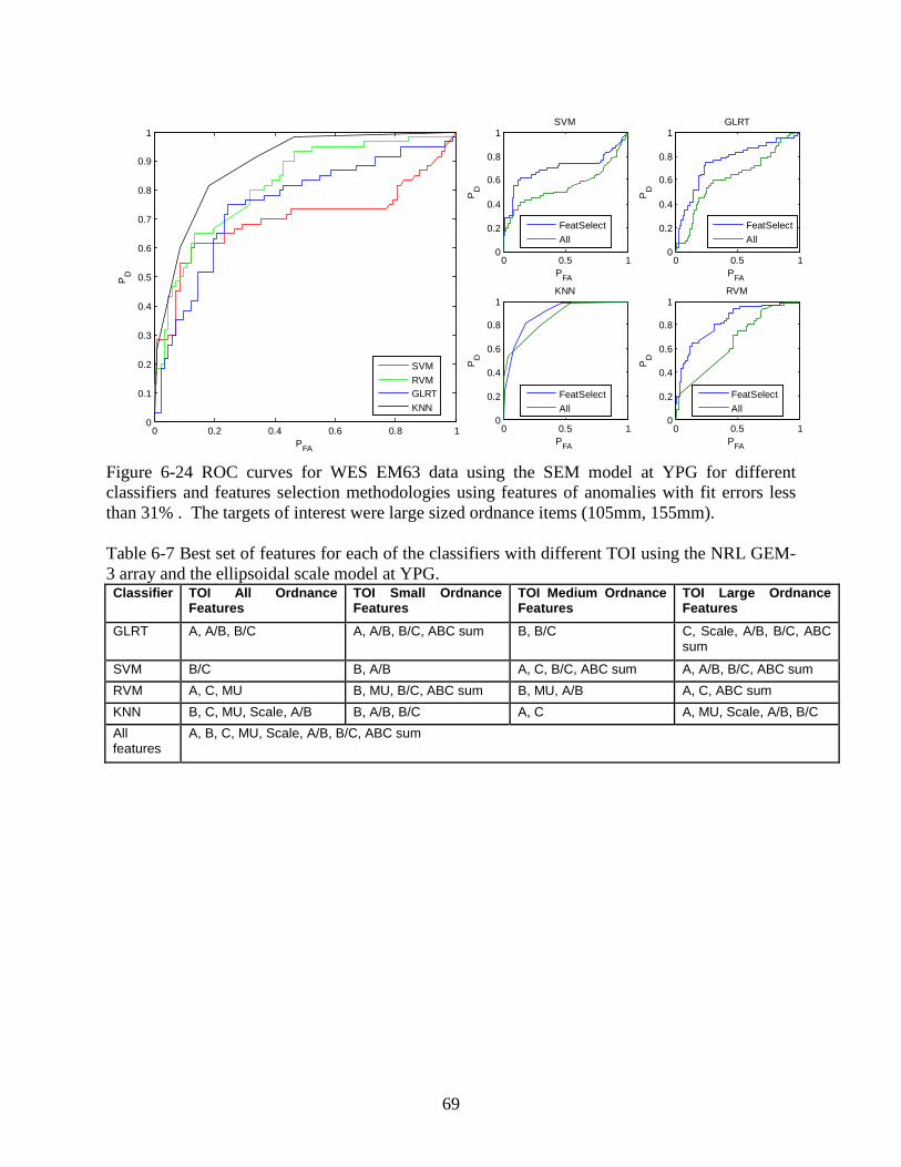
69

Figure 6-24 ROC curves for WES EM63 data using the SEM model at YPG for different classifiers and features selection methodologies using features of anomalies with fit errors less than 31% . The targets of interest were large sized ordnance items (105mm, 155mm). Table 6-7 Best set of features for each of the classifiers with different TOI using the NRL GEM-3 array and the ellipsoidal scale model at YPG. Classifier TOI All Ordnance




GLRT A, A/B, B/C A, A/B, B/C, ABC sum B, B/C C, Scale, A/B, B/C, ABC sum

SVM B/C B, A/B A, C, B/C, ABC sum A, A/B, B/C, ABC sum RVM A, C, MU B, MU, B/C, ABC sum B, MU, A/B A, C, ABC sum KNN B, C, MU, Scale, A/B B, A/B, B/C A, C A, MU, Scale, A/B, B/C All features

A, B, C, MU, Scale, A/B, B/C, ABC sum

0 0.2 0.4 0.6 0.8 10

0.1

0.2

0.3

0.4

0.5

0.6

0.7

0.8

0.9

1

PFA

PD

0 0.5 10

0.2

0.4

0.6

0.8

1

PFA

PD

SVM

0 0.5 10

0.2

0.4

0.6

0.8

1

PFA

PD

GLRT

0 0.5 10

0.2

0.4

0.6

0.8

1

PFA

PD

KNN

0 0.5 10

0.2

0.4

0.6

0.8

1

PFA

PD

RVM

SVMRVMGLRTKNN

FeatSelectAll

FeatSelectAll

FeatSelectAll

FeatSelectAll

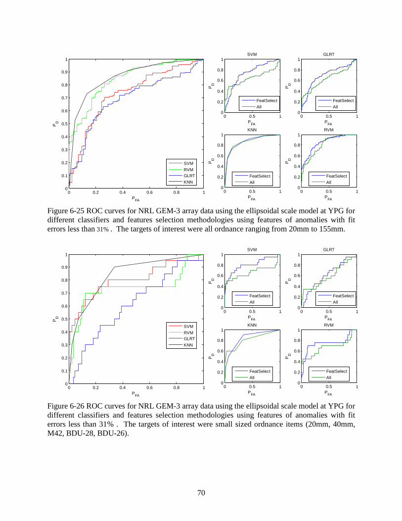
70

Figure 6-25 ROC curves for NRL GEM-3 array data using the ellipsoidal scale model at YPG for different classifiers and features selection methodologies using features of anomalies with fit errors less than 31% . The targets of interest were all ordnance ranging from 20mm to 155mm.

Figure 6-26 ROC curves for NRL GEM-3 array data using the ellipsoidal scale model at YPG for different classifiers and features selection methodologies using features of anomalies with fit errors less than 31% . The targets of interest were small sized ordnance items (20mm, 40mm, M42, BDU-28, BDU-26).

0 0.2 0.4 0.6 0.8 10

0.1

0.2

0.3

0.4

0.5

0.6

0.7

0.8

0.9

1

PFA

PD

0 0.5 10

0.2

0.4

0.6

0.8

1

PFA

PD

SVM

0 0.5 10

0.2

0.4

0.6

0.8

1

PFA

PD

GLRT

0 0.5 10

0.2

0.4

0.6

0.8

1

PFA

PD

KNN

0 0.5 10

0.2

0.4

0.6

0.8

1

PFA

PD

RVM

SVMRVMGLRTKNN

FeatSelectAll

FeatSelectAll

FeatSelectAll

FeatSelectAll

0 0.2 0.4 0.6 0.8 10

0.1

0.2

0.3

0.4

0.5

0.6

0.7

0.8

0.9

1

PFA

PD

0 0.5 10

0.2

0.4

0.6

0.8

1

PFA

PD

SVM

0 0.5 10

0.2

0.4

0.6

0.8

1

PFA

PD

GLRT

0 0.5 10

0.2

0.4

0.6

0.8

1

PFA

PD

KNN

0 0.5 10

0.2

0.4

0.6

0.8

1

PFA

PD

RVM

SVMRVMGLRTKNN

FeatSelectAll

FeatSelectAll

FeatSelectAll

FeatSelectAll

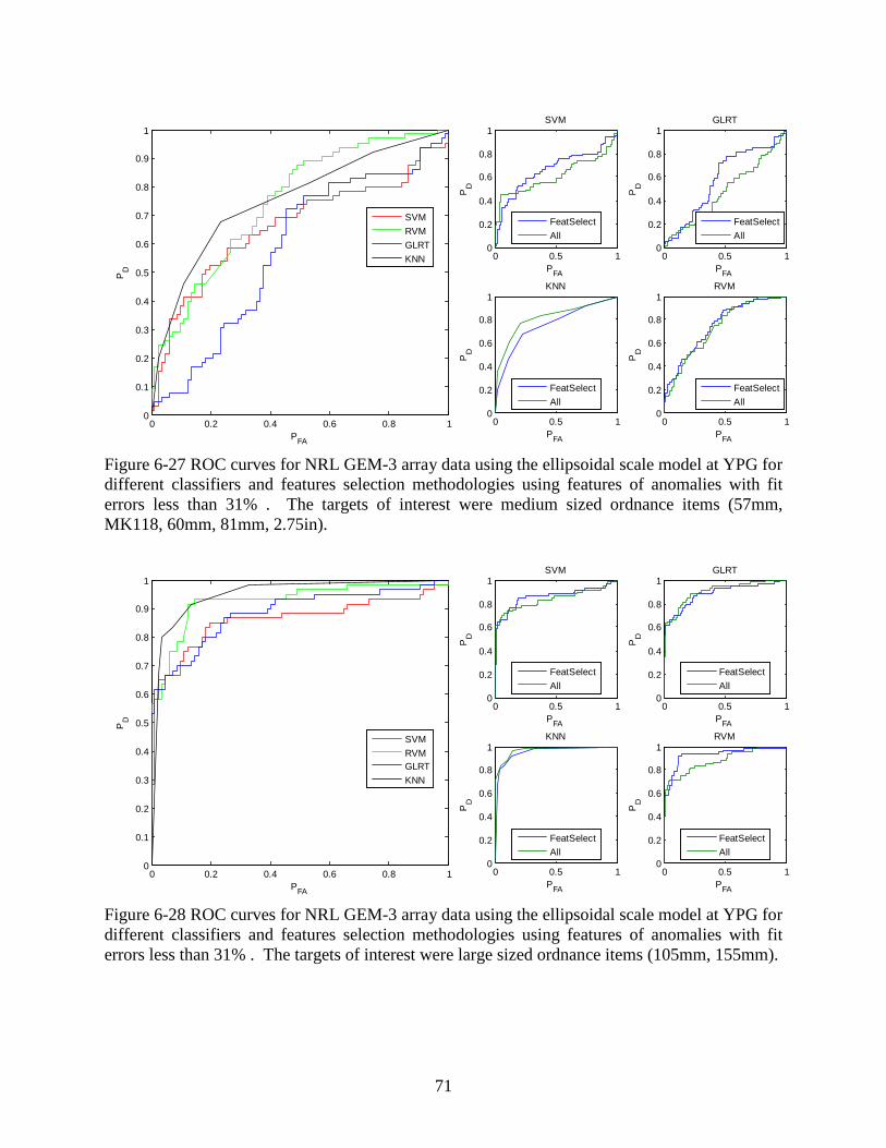
71

Figure 6-27 ROC curves for NRL GEM-3 array data using the ellipsoidal scale model at YPG for different classifiers and features selection methodologies using features of anomalies with fit errors less than 31% . The targets of interest were medium sized ordnance items (57mm, MK118, 60mm, 81mm, 2.75in).

Figure 6-28 ROC curves for NRL GEM-3 array data using the ellipsoidal scale model at YPG for different classifiers and features selection methodologies using features of anomalies with fit errors less than 31% . The targets of interest were large sized ordnance items (105mm, 155mm).

0 0.2 0.4 0.6 0.8 10

0.1

0.2

0.3

0.4

0.5

0.6

0.7

0.8

0.9

1

PFA

PD

0 0.5 10

0.2

0.4

0.6

0.8

1

PFA

PD

SVM

0 0.5 10

0.2

0.4

0.6

0.8

1

PFA

PD

GLRT

0 0.5 10

0.2

0.4

0.6

0.8

1

PFA

PD

KNN

0 0.5 10

0.2

0.4

0.6

0.8

1

PFA

PD

RVM

SVMRVMGLRTKNN

FeatSelectAll

FeatSelectAll

FeatSelectAll

FeatSelectAll

0 0.2 0.4 0.6 0.8 10

0.1

0.2

0.3

0.4

0.5

0.6

0.7

0.8

0.9

1

PFA

PD

0 0.5 10

0.2

0.4

0.6

0.8

1

PFA

PD

SVM

0 0.5 10

0.2

0.4

0.6

0.8

1

PFA

PD

GLRT

0 0.5 10

0.2

0.4

0.6

0.8

1

PFA

PD

KNN

0 0.5 10

0.2

0.4

0.6

0.8

1

PFA

PD

RVM

SVMRVMGLRTKNN

FeatSelectAll

FeatSelectAll

FeatSelectAll

FeatSelectAll

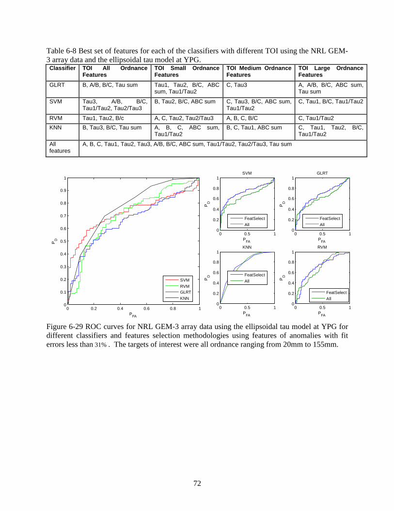
72

Table 6-8 Best set of features for each of the classifiers with different TOI using the NRL GEM-3 array data and the ellipsoidal tau model at YPG. Classifier TOI All Ordnance




GLRT B, A/B, B/C, Tau sum Tau1, Tau2, B/C, ABC sum, Tau1/Tau2

C, Tau3 A, A/B, B/C, ABC sum, Tau sum

SVM Tau3, A/B, B/C, Tau1/Tau2, Tau2/Tau3

B, Tau2, B/C, ABC sum C, Tau3, B/C, ABC sum, Tau1/Tau2

C, Tau1, B/C, Tau1/Tau2

RVM Tau1, Tau2, B/c A, C, Tau2, Tau2/Tau3 A, B, C, B/C C, Tau1/Tau2 KNN B, Tau3, B/C, Tau sum A, B, C, ABC sum,

Tau1/Tau2 B, C, Tau1, ABC sum C, Tau1, Tau2, B/C,

Tau1/Tau2

All features

A, B, C, Tau1, Tau2, Tau3, A/B, B/C, ABC sum, Tau1/Tau2, Tau2/Tau3, Tau sum

Figure 6-29 ROC curves for NRL GEM-3 array data using the ellipsoidal tau model at YPG for different classifiers and features selection methodologies using features of anomalies with fit errors less than 31% . The targets of interest were all ordnance ranging from 20mm to 155mm.

0 0.2 0.4 0.6 0.8 10

0.1

0.2

0.3

0.4

0.5

0.6

0.7

0.8

0.9

1

PFA

PD

0 0.5 10

0.2

0.4

0.6

0.8

1

PFA

PD

SVM

0 0.5 10

0.2

0.4

0.6

0.8

1

PFA

PD

GLRT

0 0.5 10

0.2

0.4

0.6

0.8

1

PFA

PD

KNN

0 0.5 10

0.2

0.4

0.6

0.8

1

PFA

PD

RVM

SVMRVMGLRTKNN

FeatSelectAll

FeatSelectAll

FeatSelectAll

FeatSelectAll

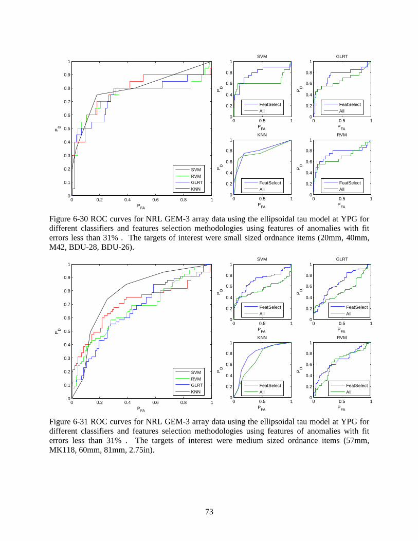
73

Figure 6-30 ROC curves for NRL GEM-3 array data using the ellipsoidal tau model at YPG for different classifiers and features selection methodologies using features of anomalies with fit errors less than 31% . The targets of interest were small sized ordnance items (20mm, 40mm, M42, BDU-28, BDU-26).

Figure 6-31 ROC curves for NRL GEM-3 array data using the ellipsoidal tau model at YPG for different classifiers and features selection methodologies using features of anomalies with fit errors less than 31% . The targets of interest were medium sized ordnance items (57mm, MK118, 60mm, 81mm, 2.75in).

0 0.2 0.4 0.6 0.8 10

0.1

0.2

0.3

0.4

0.5

0.6

0.7

0.8

0.9

1

PFA

PD

0 0.5 10

0.2

0.4

0.6

0.8

1

PFA

PD

SVM

0 0.5 10

0.2

0.4

0.6

0.8

1

PFA

PD

GLRT

0 0.5 10

0.2

0.4

0.6

0.8

1

PFA

PD

KNN

0 0.5 10

0.2

0.4

0.6

0.8

1

PFA

PD

RVM

SVMRVMGLRTKNN

FeatSelectAll

FeatSelectAll

FeatSelectAll

FeatSelectAll

0 0.2 0.4 0.6 0.8 10

0.1

0.2

0.3

0.4

0.5

0.6

0.7

0.8

0.9

1

PFA

PD

0 0.5 10

0.2

0.4

0.6

0.8

1

PFA

PD

SVM

0 0.5 10

0.2

0.4

0.6

0.8

1

PFA

PD

GLRT

0 0.5 10

0.2

0.4

0.6

0.8

1

PFA

PD

KNN

0 0.5 10

0.2

0.4

0.6

0.8

1

PFA

PD

RVM

SVMRVMGLRTKNN

FeatSelectAll

FeatSelectAll

FeatSelectAll

FeatSelectAll

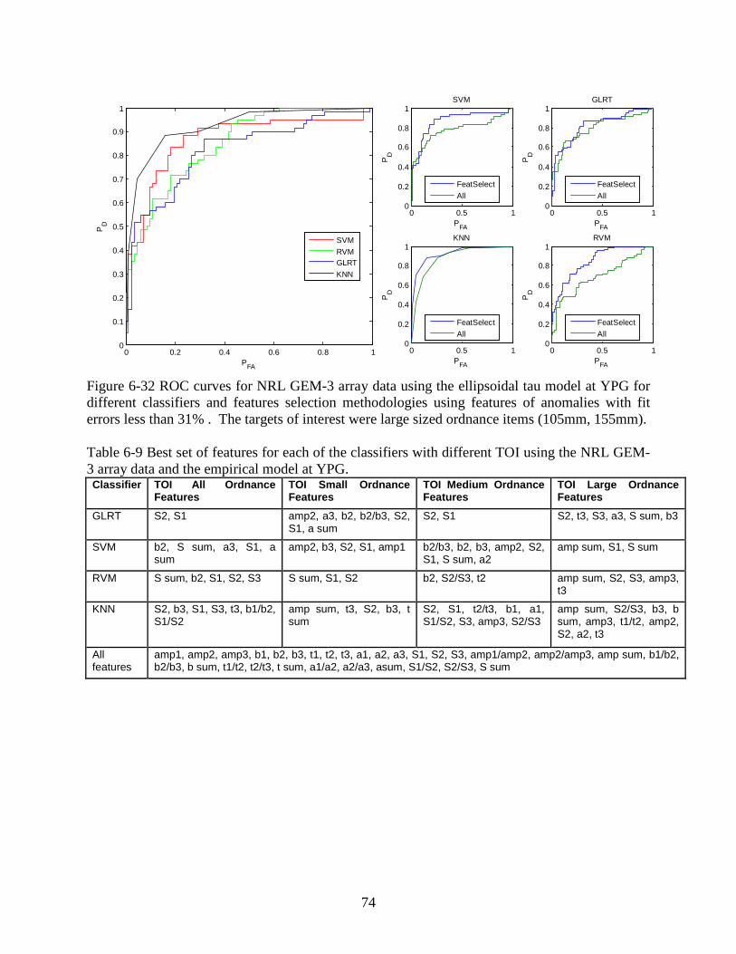
74

Figure 6-32 ROC curves for NRL GEM-3 array data using the ellipsoidal tau model at YPG for different classifiers and features selection methodologies using features of anomalies with fit errors less than 31% . The targets of interest were large sized ordnance items (105mm, 155mm). Table 6-9 Best set of features for each of the classifiers with different TOI using the NRL GEM-3 array data and the empirical model at YPG. Classifier TOI All Ordnance




GLRT S2, S1 amp2, a3, b2, b2/b3, S2, S1, a sum

S2, S1 S2, t3, S3, a3, S sum, b3

SVM b2, S sum, a3, S1, a sum

amp2, b3, S2, S1, amp1 b2/b3, b2, b3, amp2, S2, S1, S sum, a2

amp sum, S1, S sum

RVM S sum, b2, S1, S2, S3 S sum, S1, S2 b2, S2/S3, t2 amp sum, S2, S3, amp3, t3

KNN S2, b3, S1, S3, t3, b1/b2, S1/S2

amp sum, t3, S2, b3, t sum

S2, S1, t2/t3, b1, a1, S1/S2, S3, amp3, S2/S3

amp sum, S2/S3, b3, b sum, amp3, t1/t2, amp2, S2, a2, t3

All features

amp1, amp2, amp3, b1, b2, b3, t1, t2, t3, a1, a2, a3, S1, S2, S3, amp1/amp2, amp2/amp3, amp sum, b1/b2, b2/b3, b sum, t1/t2, t2/t3, t sum, a1/a2, a2/a3, asum, S1/S2, S2/S3, S sum

0 0.2 0.4 0.6 0.8 10

0.1

0.2

0.3

0.4

0.5

0.6

0.7

0.8

0.9

1

PFA

PD

0 0.5 10

0.2

0.4

0.6

0.8

1

PFA

PD

SVM

0 0.5 10

0.2

0.4

0.6

0.8

1

PFA

PD

GLRT

0 0.5 10

0.2

0.4

0.6

0.8

1

PFA

PD

KNN

0 0.5 10

0.2

0.4

0.6

0.8

1

PFA

PD

RVM

SVMRVMGLRTKNN

FeatSelectAll

FeatSelectAll

FeatSelectAll

FeatSelectAll

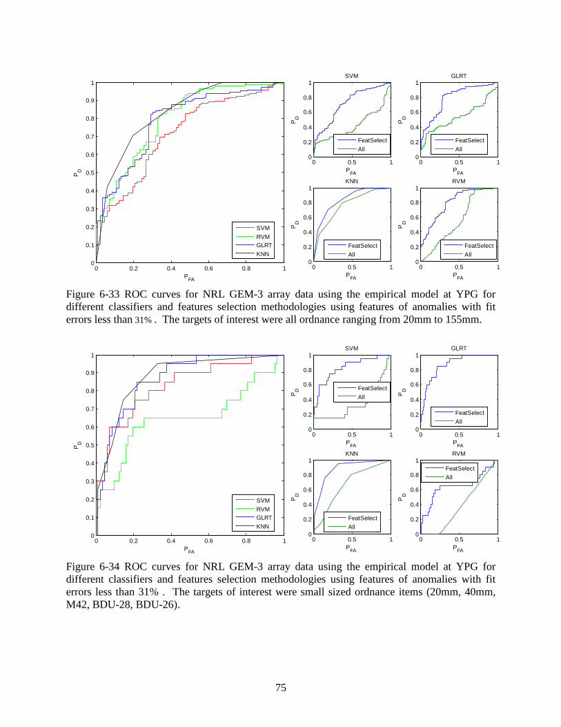
75

Figure 6-33 ROC curves for NRL GEM-3 array data using the empirical model at YPG for different classifiers and features selection methodologies using features of anomalies with fit errors less than 31% . The targets of interest were all ordnance ranging from 20mm to 155mm.

Figure 6-34 ROC curves for NRL GEM-3 array data using the empirical model at YPG for different classifiers and features selection methodologies using features of anomalies with fit errors less than 31% . The targets of interest were small sized ordnance items (20mm, 40mm, M42, BDU-28, BDU-26).

0 0.2 0.4 0.6 0.8 10

0.1

0.2

0.3

0.4

0.5

0.6

0.7

0.8

0.9

1

PFA

PD

0 0.5 10

0.2

0.4

0.6

0.8

1

PFA

PD

SVM

0 0.5 10

0.2

0.4

0.6

0.8

1

PFA

PD

GLRT

0 0.5 10

0.2

0.4

0.6

0.8

1

PFA

PD

KNN

0 0.5 10

0.2

0.4

0.6

0.8

1

PFA

PD

RVM

SVMRVMGLRTKNN

FeatSelectAll

FeatSelectAll

FeatSelectAll

FeatSelectAll

0 0.2 0.4 0.6 0.8 10

0.1

0.2

0.3

0.4

0.5

0.6

0.7

0.8

0.9

1

PFA

PD

0 0.5 10

0.2

0.4

0.6

0.8

1

PFA

PD

SVM

0 0.5 10

0.2

0.4

0.6

0.8

1

PFA

PD

GLRT

0 0.5 10

0.2

0.4

0.6

0.8

1

PFA

PD

KNN

0 0.5 10

0.2

0.4

0.6

0.8

1

PFA

PD

RVM

SVMRVMGLRTKNN

FeatSelectAll

FeatSelectAll

FeatSelectAll

FeatSelectAll

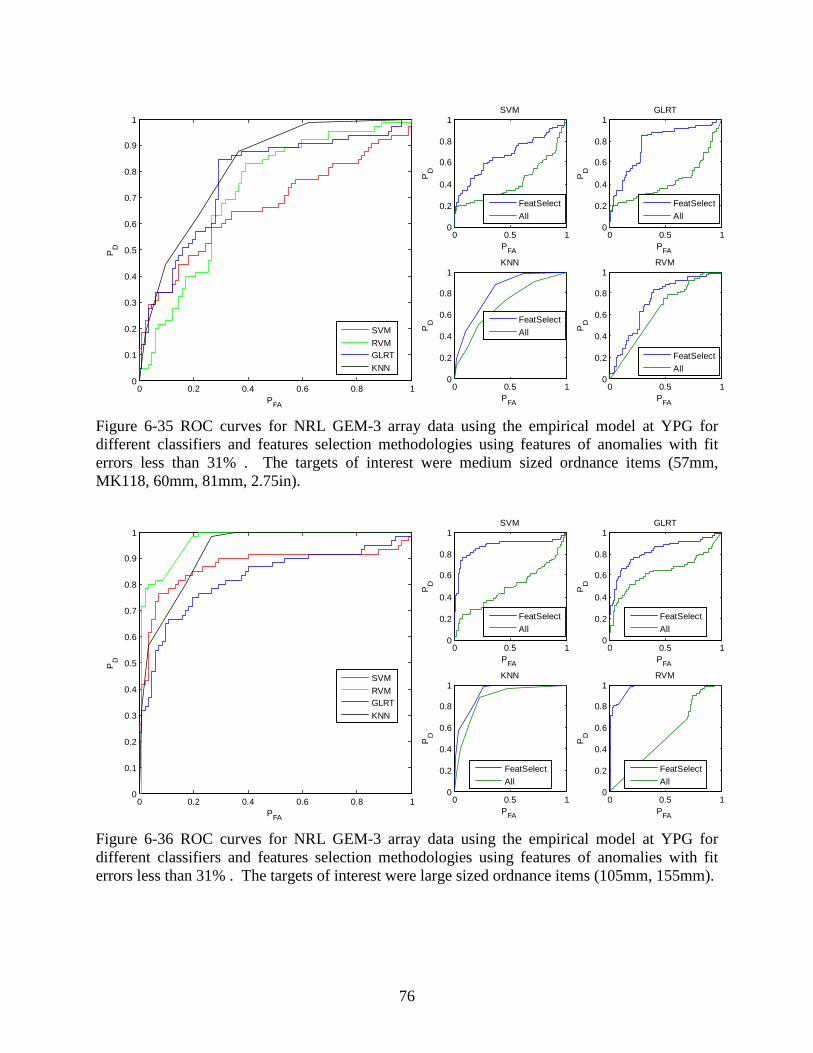
76

Figure 6-35 ROC curves for NRL GEM-3 array data using the empirical model at YPG for different classifiers and features selection methodologies using features of anomalies with fit errors less than 31% . The targets of interest were medium sized ordnance items (57mm, MK118, 60mm, 81mm, 2.75in).

Figure 6-36 ROC curves for NRL GEM-3 array data using the empirical model at YPG for different classifiers and features selection methodologies using features of anomalies with fit errors less than 31% . The targets of interest were large sized ordnance items (105mm, 155mm).

0 0.2 0.4 0.6 0.8 10

0.1

0.2

0.3

0.4

0.5

0.6

0.7

0.8

0.9

1

PFA

PD

0 0.5 10

0.2

0.4

0.6

0.8

1

PFA

PD

SVM

0 0.5 10

0.2

0.4

0.6

0.8

1

PFA

PD

GLRT

0 0.5 10

0.2

0.4

0.6

0.8

1

PFA

PD

KNN

0 0.5 10

0.2

0.4

0.6

0.8

1

PFA

PD

RVM

SVMRVMGLRTKNN

FeatSelectAll

FeatSelectAll

FeatSelectAll

FeatSelectAll

0 0.2 0.4 0.6 0.8 10

0.1

0.2

0.3

0.4

0.5

0.6

0.7

0.8

0.9

1

PFA

PD

0 0.5 10

0.2

0.4

0.6

0.8

1

PFA

PD

SVM

0 0.5 10

0.2

0.4

0.6

0.8

1

PFA

PD

GLRT

0 0.5 10

0.2

0.4

0.6

0.8

1

PFA

PD

KNN

0 0.5 10

0.2

0.4

0.6

0.8

1

PFA

PD

RVM

SVMRVMGLRTKNN

FeatSelectAll

FeatSelectAll

FeatSelectAll

FeatSelectAll

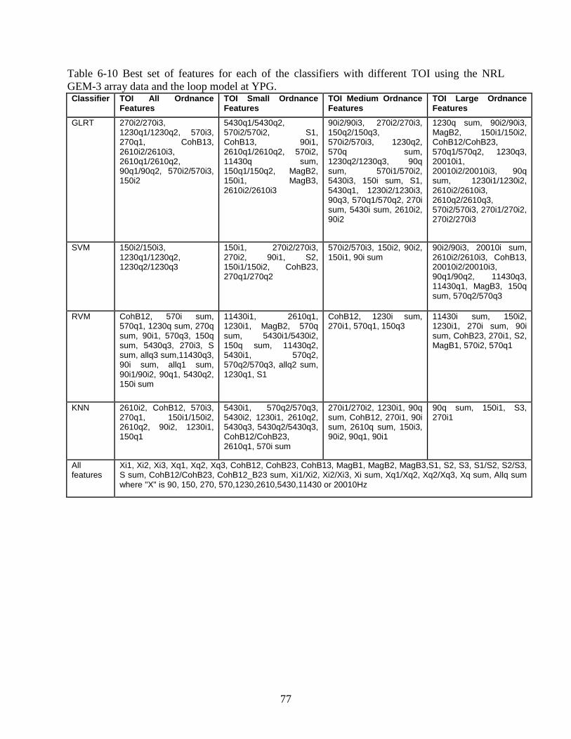
77

Table 6-10 Best set of features for each of the classifiers with different TOI using the NRL GEM-3 array data and the loop model at YPG. Classifier TOI All Ordnance




GLRT 270i2/270i3, 1230q1/1230q2, 570i3, 270q1, CohB13, 2610i2/2610i3, 2610q1/2610q2, 90q1/90q2, 570i2/570i3, 150i2

5430q1/5430q2, 570i2/570i2, S1, CohB13, 90i1, 2610q1/2610q2, 570i2, 11430q sum, 150q1/150q2, MagB2, 150i1, MagB3, 2610i2/2610i3

90i2/90i3, 270i2/270i3, 150q2/150q3, 570i2/570i3, 1230q2, 570q sum, 1230q2/1230q3, 90q sum, 570i1/570i2, 5430i3, 150i sum, S1, 5430q1, 1230i2/1230i3, 90q3, 570q1/570q2, 270i sum, 5430i sum, 2610i2, 90i2

1230q sum, 90i2/90i3, MagB2, 150i1/150i2, CohB12/CohB23, 570q1/570q2, 1230q3, 20010i1, 20010i2/20010i3, 90q sum, 1230i1/1230i2, 2610i2/2610i3, 2610q2/2610q3, 570i2/570i3, 270i1/270i2, 270i2/270i3

SVM 150i2/150i3, 1230q1/1230q2, 1230q2/1230q3

150i1, 270i2/270i3, 270i2, 90i1, S2, 150i1/150i2, CohB23, 270q1/270q2

570i2/570i3, 150i2, 90i2, 150i1, 90i sum

90i2/90i3, 20010i sum, 2610i2/2610i3, CohB13, 20010i2/20010i3, 90q1/90q2, 11430q3, 11430q1, MagB3, 150q sum, 570q2/570q3

RVM CohB12, 570i sum, 570q1, 1230q sum, 270q sum, 90i1, 570q3, 150q sum, 5430q3, 270i3, S sum, allq3 sum,11430q3, 90i sum, allq1 sum, 90i1/90i2, 90q1, 5430q2, 150i sum

11430i1, 2610q1, 1230i1, MagB2, 570q sum, 5430i1/5430i2, 150q sum, 11430q2, 5430i1, 570q2, 570q2/570q3, allq2 sum, 1230q1, S1

CohB12, 1230i sum, 270i1, 570q1, 150q3

11430i sum, 150i2, 1230i1, 270i sum, 90i sum, CohB23, 270i1, S2, MagB1, 570i2, 570q1

KNN 2610i2, CohB12, 570i3, 270q1, 150i1/150i2, 2610q2, 90i2, 1230i1, 150q1

5430i1, 570q2/570q3, 5430i2, 1230i1, 2610q2, 5430q3, 5430q2/5430q3, CohB12/CohB23, 2610q1, 570i sum

270i1/270i2, 1230i1, 90q sum, CohB12, 270i1, 90i sum, 2610q sum, 150i3, 90i2, 90q1, 90i1

90q sum, 150i1, S3, 270i1

All features

Xi1, Xi2, Xi3, Xq1, Xq2, Xq3, CohB12, CohB23, CohB13, MagB1, MagB2, MagB3,S1, S2, S3, S1/S2, S2/S3, S sum, CohB12/CohB23, CohB12_B23 sum, Xi1/Xi2, Xi2/Xi3, Xi sum, Xq1/Xq2, Xq2/Xq3, Xq sum, Allq sum where "X" is 90, 150, 270, 570,1230,2610,5430,11430 or 20010Hz

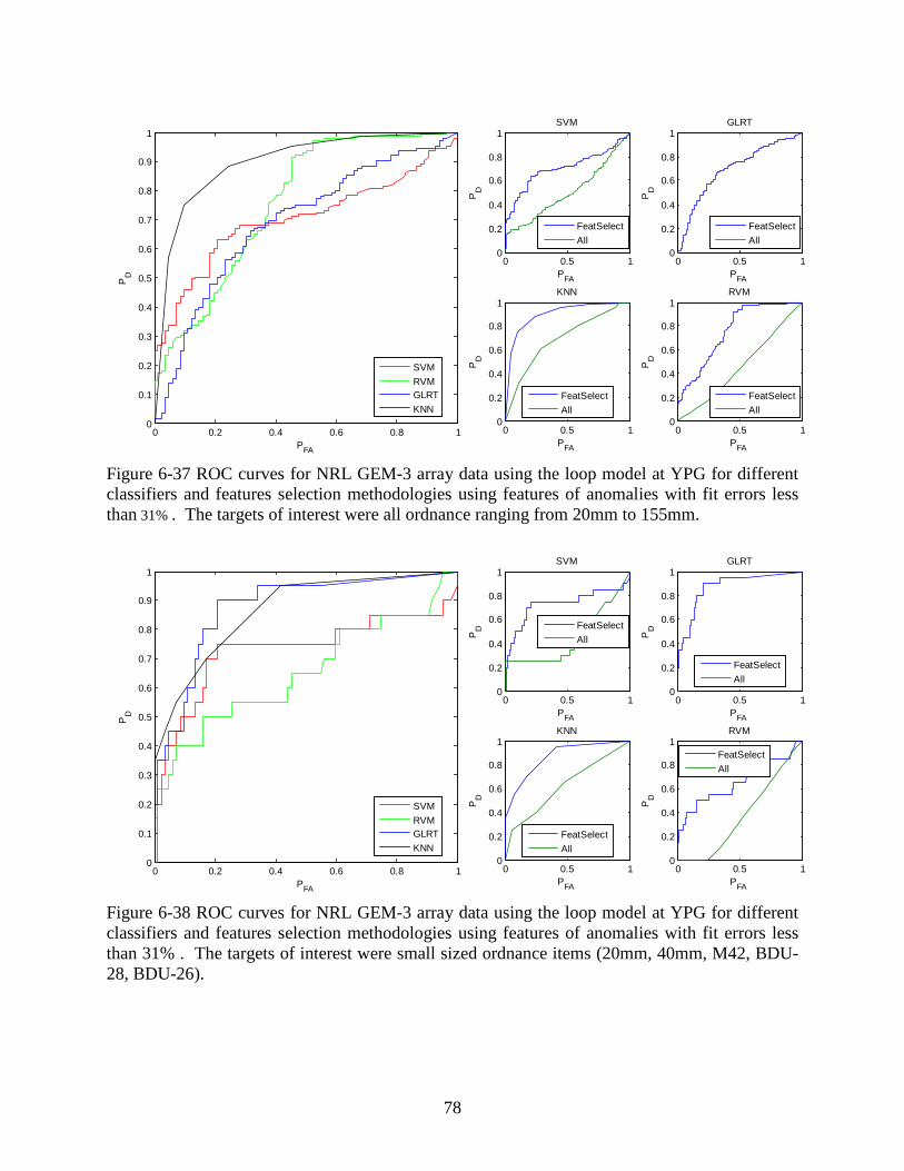
78

Figure 6-37 ROC curves for NRL GEM-3 array data using the loop model at YPG for different classifiers and features selection methodologies using features of anomalies with fit errors less than 31% . The targets of interest were all ordnance ranging from 20mm to 155mm.

Figure 6-38 ROC curves for NRL GEM-3 array data using the loop model at YPG for different classifiers and features selection methodologies using features of anomalies with fit errors less than 31% . The targets of interest were small sized ordnance items (20mm, 40mm, M42, BDU-28, BDU-26).

0 0.2 0.4 0.6 0.8 10

0.1

0.2

0.3

0.4

0.5

0.6

0.7

0.8

0.9

1

PFA

PD

0 0.5 10

0.2

0.4

0.6

0.8

1

PFA

PD

SVM

0 0.5 10

0.2

0.4

0.6

0.8

1

PFA

PD

GLRT

0 0.5 10

0.2

0.4

0.6

0.8

1

PFA

PD

KNN

0 0.5 10

0.2

0.4

0.6

0.8

1

PFA

PD

RVM

SVMRVMGLRTKNN

FeatSelectAll

FeatSelectAll

FeatSelectAll

FeatSelectAll

0 0.2 0.4 0.6 0.8 10

0.1

0.2

0.3

0.4

0.5

0.6

0.7

0.8

0.9

1

PFA

PD

0 0.5 10

0.2

0.4

0.6

0.8

1

PFA

PD

SVM

0 0.5 10

0.2

0.4

0.6

0.8

1

PFA

PD

GLRT

0 0.5 10

0.2

0.4

0.6

0.8

1

PFA

PD

KNN

0 0.5 10

0.2

0.4

0.6

0.8

1

PFA

PD

RVM

SVMRVMGLRTKNN

FeatSelectAll

FeatSelectAll

FeatSelectAll

FeatSelectAll

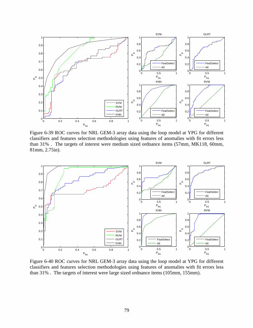
79

Figure 6-39 ROC curves for NRL GEM-3 array data using the loop model at YPG for different classifiers and features selection methodologies using features of anomalies with fit errors less than 31% . The targets of interest were medium sized ordnance items (57mm, MK118, 60mm, 81mm, 2.75in).

Figure 6-40 ROC curves for NRL GEM-3 array data using the loop model at YPG for different classifiers and features selection methodologies using features of anomalies with fit errors less than 31% . The targets of interest were large sized ordnance items (105mm, 155mm).

0 0.2 0.4 0.6 0.8 10

0.1

0.2

0.3

0.4

0.5

0.6

0.7

0.8

0.9

1

PFA

PD

0 0.5 10

0.2

0.4

0.6

0.8

1

PFA

PD

SVM

0 0.5 10

0.2

0.4

0.6

0.8

1

PFA

PD

GLRT

0 0.5 10

0.2

0.4

0.6

0.8

1

PFA

PD

KNN

0 0.5 10

0.2

0.4

0.6

0.8

1

PFA

PD

RVM

SVMRVMGLRTKNN

FeatSelectAll

FeatSelectAll

FeatSelectAll

FeatSelectAll

0 0.2 0.4 0.6 0.8 10

0.1

0.2

0.3

0.4

0.5

0.6

0.7

0.8

0.9

1

PFA

PD

0 0.5 10

0.2

0.4

0.6

0.8

1

PFA

PD

SVM

0 0.5 10

0.2

0.4

0.6

0.8

1

PFA

PD

GLRT

0 0.5 10

0.2

0.4

0.6

0.8

1

PFA

PD

KNN

0 0.5 10

0.2

0.4

0.6

0.8

1

PFA

PD

RVM

SVMRVMGLRTKNN

FeatSelectAll

FeatSelectAll

FeatSelectAll

FeatSelectAll

Documents

FINAL REPORT - Defense Technical Information Center · FINAL REPORT Advanced Signal Processing & Classification: UXO Standardized Test Site Data . SERDP Project MR-1505 . APRIL 2012