Embed Size (px)
Citation preview

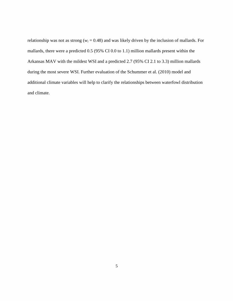
Final Report
Monitoring the Effects of Climate Change on Waterfowl Abundance in the Mississippi Alluvial Valley: Optimizing Sampling Efficacy and Efficiency
Sarah E. Lehnen
Arkansas Cooperative Fish and Wildlife Research Unit, Department of Biological Sciences, 1 University of Arkansas, Fayetteville, AR 72701

EXECUTIVE SUMMARY: Winter waterfowl surveys have been conducted across much of the
United States since 1935. Aerial surveys conducted using stratified random sampling have the
advantages of extensive coverage, increased accuracy, and the ability to calculate the variance of
estimates. A statistically robust stratified random sampling design for aerial surveys of mallards
in the Mississippi Alluvial Valley (MAV) was developed in the late 1980s and early 1990s;
surveys based on this sampling design have been conducted by the Mississippi Department of
Wildlife, Fisheries, and Parks (MDWFP) in the Mississippi MAV since 2005 and by the
Arkansas Game and Fish Commission (AGFC) in the Arkansas MAV since 2009. However,
changes in land use since the survey was designed may have made modifications of the original
design necessary. We refined strata boundaries in Arkansas using watersheds as a guide in
determining strata boundaries and surveyed the Arkansas MAV four times during winter 2011-
2012 using this modified design. To evaluate the performance of this new design we compared
three sampling designs: 1) simple random, 2) expert opinion-based strata (original design), and
3) watershed-based strata (new design). For each of the four survey periods and each of the three
sampling designs, we calculated %CV of the estimated number of mallards and total ducks by
bootstrapping the surveyed transects in each survey period 10,000 times each under each of the
three sampling designs. The %CV for all ducks and mallards was lower under the new
watershed-based stratified random sample than under either the simple random or expert-based
designs during all four survey periods. The watershed-based sampling design also estimates
waterfowl abundance at a finer resolution using biologically meaningful strata.
We also wanted to improve the accuracy of population estimates by developing a protocol to
account for biases related to observer and habitat effects on detection. We chose the double-
observer method because its relative low cost and ease of implementation made this method the

3
most feasible for agency staff. The same AGFC personal that have conducted all waterfowl
surveys in the Arkansas MAV since 2009 conducted a double-observer survey in February of
2012. These data were used to develop observer and habitat (closed or open canopy)-specific
detection probabilities for the Arkansas MAV surveys. Detection in closed canopy habitats
(obs1 =0.36, obs2=0.86) was lower than detection in open canopy habitats (obs1 =0.88,
obs2=0.99). Adjusting estimates for detection increased estimates of mallard abundance by a
mean of 27% (SE = 7%) and total ducks by 24% (SE = 7%). The large variability in the
magnitude (range 7 – 71% for all ducks) of the effect of adjustment appeared to have been due to
variation in the percentage of ducks observed in closed canopy habitat (range 3 to 32%). Because
detection was lower in closed canopy habitat, counts in closed canopy habitat had more impact
on the population estimate than the same size count in open canopy habitat.
Implementation of robust methods such as stratified random sampling can be time
consuming for agency staff. Random transects are drawn for each survey and the process of
determining randomly selected transects for each strata and each survey can take days of agency
time. This time requirement may be a limiting factor for implementation of these methods,
potentially threatening the conclusions and inferences from coordinated survey efforts, and the
long-term viability of this monitoring program. However, recent development by the Arkansas
Cooperative Fish and Wildlife Research Unit of a user-friendly, easily modifiable graphical user
interface (GUI) that rapidly selects random transects by strata and generates files for input into
computer programs and GPS units has greatly reduced the time staff spent preparing for the
surveys. Furthermore, application of this protocol to waterfowl monitoring in adjacent states
(e.g., Louisiana) has heretofore been limited, at least in part, by the support capacity for analysis.

4
This tool helps to eliminate that constraint and provide incentives for agencies to use a more
robust protocol. Even with the improved system for survey preparation, there was an additional
need to further develop the GUI to quickly process and analyze the collected survey data.
Calculations of variance in stratified random sampling can be complex; implementation of these
calculations in the GUI reduce the amount of time and statistical expertise required by users. The
inclusion of a kernel density estimator in the GUI also avoids the need for access to a GIS with
analysis capabilities. The increased speed of analysis allows for faster dissemination of survey
data, which may allow managers to provide timely information to the public and to adjust habitat
management in response to the most recent information on duck distributions. In addition, the
GUI allows for easier expansion of surveys into new regions by the inclusion of an option for the
user to upload new files from which to select random transects. Expansion of these surveys into
neighboring regions would increase the capacity for distinguishing distribution shifts from
population changes.
Given the potential for changes to wildlife distribution and abundance under various
climate change scenarios, there is a need to better understand the effects of climate on waterfowl
distributions. We evaluated the cumulative winter severity index (WSI) developed by Schummer
et al. (2010) to predict waterfowl abundance using data collected in Arkansas during winters
2009-2011. For dabbling ducks other than mallards, no model performed better than the null and
only models containing year had strong support for diving ducks. The best model for predicting
mallard abundance contained the WSI for the Arkansas MAV (wi = 0.88). Mallards occurred in
higher numbers when the weather conditions within the MAV were more severe. Number of all
ducks combined also had a positive relationship with the WSI in the MAV but evidence for this
5
relationship was not as strong (wi = 0.48) and was likely driven by the inclusion of mallards. For
mallards, there were a predicted 0.5 (95% CI 0.0 to 1.1) million mallards present within the
Arkansas MAV with the mildest WSI and a predicted 2.7 (95% CI 2.1 to 3.3) million mallards
during the most severe WSI. Further evaluation of the Schummer et al. (2010) model and
additional climate variables will help to clarify the relationships between waterfowl distribution
and climate.

6
Introduction
Given the potential for changes to wildlife distribution and abundance under various
climate change scenarios, there is a need to effectively and efficiently collect indices of these
metrics for wildlife populations. Wintering waterfowl, in particular, provide an excellent
bellwether for the effects of climate change as changes in their abundance and distribution reflect
both a direct response to climatic variables (e.g., temperature and precipitation) and an indirect
response to climate change mediated through habitat alterations. The mallard (Anas
platyrhynchos) is the most abundant (and arguably most popular for sport) duck in North
America, and their numbers are often used as a surrogate to gauge the health of other waterfowl
populations and in making management decisions (U. S. Dep. Int. and Envrion. Canada 1986,
Drilling et al. 2002). The Mississippi Alluvial Valley (MAV) is an area of continental
significance for migrating and wintering waterfowl under the auspices of the North American
Waterfowl Management Plan (NAWMP 2012), and the single most important region for
wintering mallards (Reinecke et al. 1989). Therefore, MAV-wide monitoring of mallards and
other duck species has the potential to provide some of the earliest indications of climate change
impacts on wildlife.
Winter waterfowl surveys have been conducted across much of the United States since
1935. Many different counting techniques have been used, but aerial waterfowl surveys have the
advantages of 1) the ability to survey areas difficult to access by ground, 2) the ability to rapidly
survey large regions, and 3) the elimination of double counting by traveling faster than
waterfowl can fly. However, sampling designs have generally relied on professional judgment of

7
areas believed to be important to waterfowl rather than statistical probability to establish
“representative” samples, making inferences and comparisons of estimates within and among
years and geographic regions difficult. In response to these challenges, Reinecke et al. (1992)
developed a statistically-robust, stratified random sampling design for aerial surveys of mallards
in the MAV during the late 1980s and early 1990s. Surveys in the MAV conducted using
stratified random sampling of aerial fixed-width strips can be used to estimate population size
and precision of estimates for large regions; these estimates can be compared among regions and
over time. Using a stratified design rather than a simple random design allows the researchers to
allocate more effort to areas with expected higher numbers of ducks and larger variances;
whereas, areas with low numbers of ducks and little variance are sampled at a lower rate.
Beginning in 2005, the Mississippi Department of Wildlife, Fisheries and Parks, in cooperation
with Mississippi State University, has annually conducted aerial surveys following a
modification of this protocol and estimated abundance and distribution of mallards four times
each winter (Pearse et al. 2008a, 2008b). Based on that success, the Arkansas Game and Fish
Commission (AGFC) adopted the Reinecke et al. (1992) protocol for its aerial surveys of the
Arkansas portion of the MAV and, beginning in November 2009, conducted four waterfowl
surveys each winter.
However, these waterfowl surveys are complicated by the high degree of variability
associated with the clumped distribution of birds and the often ephemeral nature of the habitats
they use; precipitation and wetland conditions vary within and among years leading to highly
dynamic usage of habitat by waterfowl (Reinecke et al. 1992). Additionally, not all birds present
within the surveyed region are detected during aerial surveys and the proportion of birds not seen

8
may vary by habitat type, group size, and observer (Smith et al. 1995, Pearse et al. 2008a). These
challenges can result in population indices with high variances, making it difficult to detect
changes in population size or distribution. Pearse et al. (2008a,b) refined the sampling design of
Reinecke et al. (1992) and Smith et al. (1995) to better reflect the current landscape conditions in
the MAV, including distribution of waterfowl and waterfowl habitat (e.g., established a high-
density strata where new waterfowl habitat exists that was not present 20 years prior). This
refinement has allowed for more efficient allocation of sampling effort and provides precise
estimates of waterfowl abundance in the Mississippi MAV. Similar landscape changes have
likely occurred across the MAV, particularly in Arkansas and Louisiana, since the original
sampling design was developed, creating the need to reevaluate the current sampling design in
the Arkansas MAV and revisit the original design in the Louisiana MAV.
In addition to redeveloping strata design, addressing the issue of incomplete detection,
that is, waterfowl present in the surveyed transects but not detected by observers, may reduce
variance and improve the accuracy of the population estimates. It is well established that bias
may result from incomplete detection during aerial surveys (Caughley 1974, Caughley 1977).
Smith et al. (1995) and Pearse et al. (2008a) recognized that surveying waterfowl in the MAV
was complicated by differences in visibility due to habitat types, primarily forested wetlands
versus croplands, and due to group sizes of ducks counted. Visibility Correction Factors (VCFs)
were developed by Pearse et al. (2008a) to account for these biases but those VCFs were survey-
specific because of variation in habitat and observer effects. Given limited funds and staff time, a
simple and cost effective means of estimating detection is needed that can be used by agency
staff to adjust population estimates. A double-observer approach (Nichols et al. 2000) is one

9
potential cost-effective solution that has been used in waterfowl surveys (Koneff et al. 2008,
Vrtiska and Powell 2011).
One draw-back of the implementation of robust methods such as stratified random
sampling is the time required by agency staff to process files for input and the compile and
analyze the collected data. New random transects are drawn for each survey and the process of
determining randomly selected transects for each strata and each survey can take days of agency
time. The transects selected must also be processed in order to be read into computer programs
and GPS units. The time required of agency staff to implement these survey protocols may limit
use of this survey method, potentially threatening the conclusions and inferences from
coordinated survey efforts, and the long-term viability of this monitoring program. However,
recent development by the Arkansas Cooperative Fish and Wildlife Research Unit of a user-
friendly, easily modifiable graphical user interface (GUI) that rapidly selects random transects by
strata and generates files for input into computer programs and GPS units has greatly reduced the
time staff spent preparing for the surveys. Furthermore, application of this protocol to waterfowl
monitoring in adjacent states (e.g., Louisiana) has heretofore been limited by the scientific
support capacity for analysis. This tool helps to eliminate that constraint and provide incentives
for agencies to use a more robust protocol. There is additional need to develop the GUI to
quickly process and analyze the collected survey data. Calculations of variance in stratified
random sampling can be complex; implementation of these calculations in the GUI would reduce
the amount of time and statistical expertise required by users. Examples of these calculations
include bootstrapping estimates of variance and the production of kernel density estimates. The
development of an analysis component to the GUI will allow agency staff to determine duck

10
abundance and distribution within surveyed regions shortly after observers tabulate the survey
data. Faster dissemination of survey results will better inform managers of current waterfowl
distributions, allow quicker dissemination of information to the public and may allow managers
to better respond to waterfowl needs.
Waterfowl survey data collected in the MAV can be used to complement ongoing work to
develop models of future duck distributions using weather severity thresholds and long-term
changes in weather severity (Schummer et al. 2010). The data collected under a coordinated
MAV waterfowl monitoring framework would be valuable for cross-validation of these model
predictions. These data also would be useful in combination with ongoing efforts to model the
impacts of precipitation, climate, and land use on the surface-water system within select MAV
watersheds by providing an index of waterfowl population response to hydrologic variables
presumed to be key drivers of waterfowl distribution and abundance.
Objectives:
1) Refine strata boundaries in Arkansas and expand surveys to other states in the MAV.
Precisely (coefficient of variation [CV] ≤ 15%) estimate populations of wintering ducks
(i.e., mallards, other dabbling ducks, diving ducks) during winter 2011-2012.
2) Assess the feasibility of developing a reliable and cost-effective method for estimating
detection during waterfowl aerial surveys.
3) Develop a rapid method of estimating populations and using GIS for displaying
waterfowl distribution and abundance from aerial survey data.
4) Evaluate the Schummer et al. (2010) model for predictive ability using the data collected
in Arkansas during winters 2009-2011.

11
Study Area
The MAV is the floodplain of the lower Mississippi River, covering 10 million ha of primarily
agricultural habitats. Portions of seven states lie within the boundaries of the MAV but four
states (Arkansas (3.7 million ha), Louisiana (2.9 million ha), Mississippi (1.9 million ha), and
Missouri (1.0 million ha)) comprise over 96% of the total area. Historically, the MAV was
dominated by bottomland hardwood forest and flooded frequently during the spring and fall
(Reinecke et al. 1989). Extensive clearing during the 19th and 20th centuries have transformed
this region into an area dominated by agriculture; in addition, flood control projects have greatly
altered natural hydrology (Galloway 1980). Despite these alterations, the MAV remains a
continentally important region for migrating and wintering waterfowl, particularly mallards
(Reinecke et al. 1989). Currently, flooded agricultural fields (primarily rice and soybeans)
provide much of the foraging habitat for waterfowl in the region (Stafford et al. 2006). The
mallard is the most abundant duck species in the MAV during winter. Other dabbling duck
species common in the region during winter include, roughly in order of abundance, northern
pintail (Anas acuta), northern shoveler (A. clypeata), gadwall (A. strepera), American green-
winged teal (A. crecca), blue-winged teal (A. discors), American wigeon (A. americana), and
wood duck (Aix sponsa) (L.W. Naylor, Arkansas Game and Fish Commission, personal
communication). Diving ducks are much less abundant than dabbling ducks in the MAV and
primarily use lakes, rivers, and aquaculture ponds rather than flooded agricultural fields.
Common species of diving duck in the MAV during winter include bufflehead (Bucephala
albeola), canvasback (Aythya valisineria), hooded merganser (Lophodytes cucullatus), ring-

12
necked duck (Aythya collaris), and lesser scaup (Aythya affinis) (L.W. Naylor, Arkansas Game
and Fish Commission, personal communication).
Methods
Refine strata boundaries in Arkansas and expand surveys to other states in the MAV. One
of our main objectives was the reduction of %CV of the waterfowl surveys. With Luke Naylor
(AGFC), we redesigned the Arkansas MAV strata based on cataloguing unit-level watershed
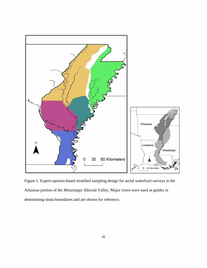
boundaries (hydrologic unit code 8) in the region. The original five strata boundaries (Figure 1)
were based on expert opinion given the best information available at the time (Reinecke et al.
1992); major rivers were also used as guides in determining strata boundaries. Because
waterfowl are closely associated with surface water availability and surface water availability is
likely to be similar within watersheds, we developed an alternative design of eleven strata based
on watershed boundaries (Figure 2). We used this new strata design during the winter 2011-2012
seasons. We used a similar watershed-based method in determining new strata boundaries for
Louisiana although the new watershed-based strata boundaries were similar to the original
boundaries created by Reinecke et al. (1992) with the exception that the northern two strata in
the old design were combined into one in the watershed-based design (Figure 3).
To evaluate the performance of this new design we compared three sampling designs: 1)
simple random, 2) expert opinion-based strata (original design; Figure 1), and 3) watershed-
based strata (new design; Figure 2). We used the data collected during winter 2011-2012 for the
comparison. For each of the four survey periods and each of the three sampling designs, we
calculated %CV of the estimated number of mallards and total ducks. We bootstrapped the

13
surveyed transects in each survey period 10,000 times each under each of the three sampling
designs. We set the total sampling effort (the total length of transects sampled) equal among the
sampling designs. For the random sample, the strata within which the data were collected were
resampled such that all areas within the Arkansas MAV had the same coverage (i.e. 8.3%
coverage in all strata). For the expert-opinion-based design, each transect in the surveys was
reassigned to one of the original strata. Because strata in the new design were generally nested
within strata in the old design this process was generally straightforward but in the event that a
transect crossed strata boundaries of the old design it was assigned to the transect in which it had
the most length. The transects were then resampled using the same relative sampling effort
among strata as in the expert design but setting the total sampling effort identical to that of the
random design. For the watershed-based design we resampled the transects 10,000 times. For
each sampling design and each survey we calculated the median %CV value out of the 10,000
bootstraps.
Detection Probabilities and Corrected Population Estimates. To assess the impact that
missed birds have on estimated waterfowl numbers, we assisted the AGFC in designing a survey
to estimate detection rates by observer and canopy cover. Detection rates in this case are the
probability of observers recording a duck, given that it is: 1) present in the surveyed region, and
2) available for detection. These detection rates may overestimate true detection because they do
not account for birds that are present but unavailable (e.g. ducks obscured by habitat such that
they are not visible from the plane). Previous work has established the importance of observer to
detection probabilities during aerial surveys (Koneff et al. 2008). In addition, we believed habitat
could influence the ability of observers to detect ducks (Smith et al. 1995, Pearse 2008b).

14
Therefore, our goal was to develop a sampling protocol that allowed us to estimate detection
rates by observer and habitat type.
We used a double-observer survey with on-the-fly-reconciliation to estimate detection
(Koneff et al. 2008, Vrtiska and Powell 2011). An earlier attempt at double sampling using two
separate planes raised issues of reconciling observations in habitat where ducks did not occur in
clearly delineated groups. In addition, it was difficult for the pilots of the two separate planes to
survey exactly the same 250-m strip of habitat. Also, birds may have moved during the lag time
between the two planes passing over the same location. In the double-observer method, both
observers were in the same plane simultaneously surveying the same habitat. These two
observers were the same observers who had conducted all the surveys in the Arkansas MAV
during the winter 2009 to 2011 surveys and who had been conducting aerial waterfowl surveys
since 2005 and 2008. To the extent possible, survey methodologies were the same in this double-
observer survey as during the regular winter surveys. At the start of each transect, one observer
took on the role of the primary observer. The primary observer called out all ducks (mallards,
divers, teal, and non-mallard dabblers) observed in the same manner as he would normally
record them using the United States Fish and Wildlife Service (USFWS), aka Hodges, “Record”
program. The primary observer called out the species or group, number observed, and habitat.
The secondary observer then recorded the observations called out by the primary observer. In
addition, the secondary observer recorded whether he also observed the group and recorded any
additional ducks he detected that were not called out by the primary observer. The primary
observer could not hear what the secondary observer was recording. Observers switched roles for
each transect, so that they served as primary and secondary observers an equal number of times.

15
AGFC personal surveyed a subset of the Arkansas MAV that was representative of the overall
habitat using one of the same planes used in the 2009 to 2011 winter surveys.
In addition to observer, other covariates could influence the detection of ducks. Although
there are a variety of habitat types within the MAV, based on previous research, we believed that
canopy cover was likely to have the strongest effect on detection (Smith et al. 1995, Pearse et al.
2008a). To account for other possible sources of heterogeneity in detection probabilities we also
included species group (mallard, teal, other dabbling ducks, or diving ducks) and group size as
covariates in the candidate model set (Table 1). We ran all models using the ‘multinomPois’
function in the ‘unmarked’ package (Fiske and Chandler 2011) within program R (R Core Team
2012). This function fits a multinomial-Poisson mixture model to data collected using double
observer sampling and allows us to compare multiple possible sources of heterogeneity in
detection probabilities. Models were ranked using AIC and the detection estimates from the top-
ranked model were used to calculate bias-corrected population estimates for the Arkansas MAV.
To determine the impact of using the bias-corrected population estimate, we calculated the
correlation coefficient (r) value of the bias-correction population estimate relative to the
uncorrected population estimates (or Population Index).
We used bootstrap resampling (Efron 1979) to estimate 95% confidence intervals, an
accepted procedure for computing variance in complex surveys. The bootstrap uses multiple
independent resamples from a sample to estimate properties of the population from which the
sample was drawn (Efron and Tibshirani 1993). We resampled transects using the original and
detection-adjusted counts 5,000 times; the lower and upper 95% confidence intervals of

16
estimated population sizes were taken from the lowest 125th and highest 4,875th of the estimated
population sizes.
Develop a rapid method of using GIS for displaying waterfowl distribution. We modified
a previously created GUI in R that could quickly select random transects for surveys and also
quickly analyze the collected data. The advantages of using a GUI are that: 1) no special
statistical programming knowledge is required by users, and 2) the software involved is open-
source, meaning that it can be easily installed on any system without requiring expensive
software licenses. Estimates of variance in stratified random sampling can also be computational
complex so use of this GUI reduces the amount of time and statistical expertise required by
users. We added additional features to the GUI such as the ability to create kernel density
estimates, a data check to locate errors in data input, the ability to estimate abundance and
variance by species group (e.g., all ducks combined), the ability to correct numbers of ducks
observed for detectability, and generated a shapfile of the transects when new random transects
were selected. We also added the Louisiana strata design to the GUI and added an option for the
user to upload new transect files for new survey designs.
Evaluate the Schummer et al. (2010) model. We developed models predicting the
relationships between duck abundance in the Arkansas MAV and Winter Severity Index (WSI)
(Schummer et al. 2010). We used the detection-corrected estimates of population of mallards,
dabbling ducks other than mallards, diving ducks, and all ducks combined in the 12 surveys
conducted between Nov 2009 and Jan 2012 as the response variable. Weather data were obtained
from Historical Climate Network (Williams et al. 2006) weather stations across the MAV
(Corning, Pocahontas, Newport, Brinkley, and Pine Bluff, Arkansas) and at weather stations at a

17
latitude of ~38 to 39ºN (Kansas City and St. Louis Missouri and Louisville, Kentucky). We
chose this latitude because it had previously been shown to influence wintering ducks in the
MAV (Pearse 2007). We initially included ambient temperature, difference in ambient
temperature between MAV and northern region, and difference in WSI between MAV and
northern region. After examining the explanatory variables for correlation, only the difference
between WSI in the MAV and northern region had a correlation below 0.7 with WSI in the MAV
so only these two variables and month and year were included in the candidate set. We fit linear
models in program R and compared them using Akaike’s Information Criteria adjusted for small
sample sizes (AICc ;Akaike 1973).
Results
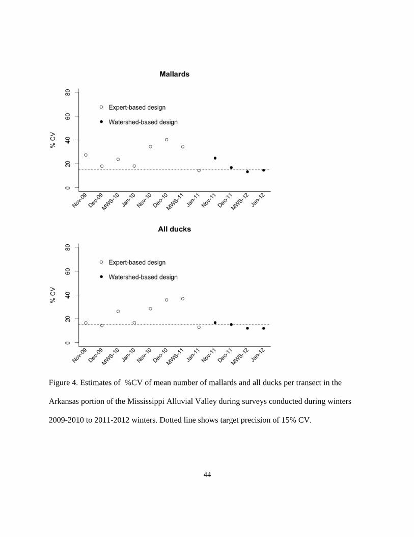
Evaluate, design and conduct aerial surveys. The mean %CV for all ducks in the
Arkansas MAV was lower during the four surveys conducted during winter 2011-2012 under the
new strata design (14.0 %CV (SE 1.18)) than it had been under the eight surveys conducted
under the old design (23.5 %CV (SE 3.42)) during winters 2009-2010 to 2010-2011. The mean
%CV for mallards was also lower under the new design (17.4 %CV (SE 2.57)) during winter
2011-2012 than under the older design (26.3 %CV (SE 3.30); Figure 4) during winters 2009-
2010 to 2010-2011. However, estimates of variance can vary among surveys for many reasons
and sampling effort was slightly higher under the new design. Using the bootstrapping procedure
to explicitly test the effect of sampling design, the %CV for all ducks and mallards was lower
under the new watershed-based stratified random sample than under either the simple random or
expert-opinion-based designs during all four survey periods (Table 2).

18
Due to constraints in the availability of personal and flight time, only one survey was
conducted in Louisiana during the winter 2011-2012 during early January 2012. There were an
estimated 372,990 (SE 33,449 95% CI 211,524 – 614,960) ducks in the Louisiana portion of the
MAV. The most common duck species was the mallard with an estimated 139,998 (SE 3,980
95% CI 76,810 to 221,381) mallards in the region.
Detection Probabilities and Corrected Population Estimates. Arkansas Game and Fish
personal surveyed 24 transects totaling 452 km in length using the double observer method on 21
February 2012. Observers recorded 166 duck groups (Table 3) of which 24 were in closed
canopy habitat, primarily bottomland hardwood forest, and the remaining 142 were in open
canopy habitat. The mean group size was 30.9 (SE 3.80) ducks with a mean group size of 35.0
(SE 4.34) ducks observed in open canopy habitat and a mean group size of 6.6 (SE 1.54) ducks
observed in closed habitat. The variables observer and canopy cover had strong support (Table
4). Not surprisingly, detection in closed canopy habitat was lower than detection in open canopy
habitat (0.86 and 0.36 in closed canopy vs. 0.99 and 0.88 in open canopy for observers 1 and 2,
respectively; Table 5).
Adjustment using observer and habitat-specific detection probabilities increased
estimates of mallard abundance by a mean of 27% (SE = 7%), other dabbling ducks by 23% (SE
= 7%), diving ducks by 12% (SE = 1%), and total ducks by 24% (SE = 7%; Table 6). The
degree of increase was related to the number of ducks observed in forested wetlands (closed
canopy habitat) during the surveys. For mallards, there was a wide range in the percent of ducks
observed in closed canopy habitat from a low of 3% in November of 2009 to a high of 32% in

19
December of 2010 (see Appendix A for additional habitat use information). For overall duck
observations the results were similar, with a low of 3% of ducks observed in closed canopy
habitat during the November 2009 survey to a high of 27% of all ducks observed in closed
canopy habitat during December of 2010. Although there was substantial variation in the
magnitude of the impact of the detection-adjustment among surveys, for mallards, other dabbling
ducks, diving ducks, and all ducks combined, there was a high degree of overlap in the 95%
confidence intervals around both the population index and the detection-adjusted population
estimate for all surveys (Figures 5, 6, 7, and 8).
Develop a rapid method of using GIS for displaying waterfowl distribution. We created a
GUI in R that could quickly select random transects for surveys and also quickly analyze
collected data (Appendix B). The GUI includes the option of creating user-defined duck groups
(e.g, all ducks combined) that can then be used for kernel density estimates and/or for estimating
strata and MAV-level populations. The GUI also includes the option of adjusting observed ducks
for observer and habitat (open or closed canopy)-level detection probabilities. The detection
probabilities from the double observer trial in the Arkansas MAV are provided as default values
but these values can be modified by the user. Along with estimates of population size, the GUI
estimates SE of MAV-wide and strata-level population estimates and uses bootstrapping to
estimate 95% confidence intervals around estimates. The analysis output also includes a
summary of ducks observed by species and habitat type and a summary of ducks observed by
species and transect.
20
Evaluate the Schummer et al. (2010) model. The best model for predicting mallards was
the model containing the WSI for the MAV (wi = 0.88; Table 6). Mallards occurred in higher
numbers when the weather conditions within the MAV were more severe (Figure 9). All ducks
combined also had a positive relationship with the WSI in the MAV but evidence for this
relationship was not as strong (wi = 0.48). For mallards, there were a predicted 0.5 (95% CI 0.0
to 1.1) million mallards present within the Arkansas MAV during the mildest WSI and a
predicted 2.7 (95% CI 2.1 to 3.3) million mallards during the most severe WSI. For all ducks,
there were a predicted 1.9 (95% CI 0.9 to 2.8) million ducks under the mildest observed WSI and
a predicted 3.8 (95% CI 2.9 to 4.7) million ducks predicted under most severe observed WSI. For
dabbling ducks other than mallards, no model performed better than the null and only models
containing year had strong support for diving ducks.
Discussion
We redesigned survey strata in the Arkansas MAV based on watershed boundaries. In
addition to having a lower %CV for both mallards and all ducks combined during all four
surveys, the watershed-based sampling design allows for a finer resolution of waterfowl
abundance estimation by being able to precisely estimate abundance in eleven biologically
meaningful strata. Watersheds are delineated across the U.S. at multiple scales, enabling this
sampling design to be readily adapted by other waterfowl researchers. The estimation of strata-
specific populations can also be used to evaluate the impacts of land use characteristics and
hydrologic processes on waterfowl abundance at the watershed level.
Incomplete detection in aerial surveys can result from factors that obstruct the view of
individuals (e.g., Smith et al. 1995) and from differences in observer’s ability to detect

21
individuals (e.g., Koneff et al. 2008). Advantages of the double observer method we used to
estimate detection probabilities are that it does not require coordination with ground crews and
avoids the issue of assuming that ground crews have perfect detection. Other studies have used
decoys to estimate detection (e.g., Pearse et al. 2008). However, observers may develop search
images for waterfowl based on cues of duck presence such as rings or ripples in water, muddy
water and the motion and color contrast of flapping wings (L. Naylor, AGFC, personal
communication); these cues would be absent in the case of decoys. In addition, implementation
of this method is fairly straight-forward and lower cost than alternatives such as ground counts or
flushing with helicopters (Koneff et al. 2008).
One drawback of this method is that it does not account for ducks that are not available
for detection, that is, ducks that are present in the surveyed region but not visible from the plane,
perhaps because of obstruction by vegetation or land features. Knoeff et al. (2008) suggested that
availability bias was a larger contributor to overall detection bias than the visibility bias
corrected for using the double-observer survey approach in their surveys of waterfowl in
southwest Ontario and the Ottawa and St. Lawrence River valleys. One approach that has
potential for estimating true detection is the combined distance and double-observer method
(Buckland et al. 2010). Discussion with observers however raised concerns over the ability to
estimate distance precisely because of slight variations in flight altitude, the lack of clear
distinctness between duck groups, and the logistical challenges of estimating an additional
parameter to an already demanding survey protocol. Replicate sampling such as ground counts
and helicopter flushing are alternative methods of estimating true detection but these methods
may be prohibitively expensive and have their own limitations in terms of bird movement on and

22
off the survey transect between aerial and replicate surveys (Knoeff et al. 2008). These methods
also assume 1) perfect detection of waterfowl by ground crews or helicopter surveys, 2) that
replicate surveys cover the same waterfowl populations as aerial surveys (e.g. zero flight path
error and no movement of waterfowl off or on survey transects between surveys), and 3) that the
replicate surveys adequately represent the entire surveyed region (Prenzlow and Lovvorn 1996).
Further application of the double-observer method would allow for more precise
estimates of detection and may allow for changes in observer-specific detection over time. In
addition, we estimated detection for all forested wetland habitat combined, which includes
cypress-tupelo, shrub-scrub wetlands, and bottomland hardwood forests. Smith et al. (1995)
estimated detection separately for these three different types of forested wetland. More habitat-
specific estimates of detection may improve the precision of estimates.
The use of the detection-adjustment increased estimates of mallard abundance by a mean
of 27% (SE = 7%), other dabbling ducks by 23% (SE = 7%), diving ducks by 12% (SE = 1%),
and total ducks by 24% (SE = 7%). The large variability among years appeared to have been due
to the variation in the percentage of ducks observed in closed canopy habitat, which ranged from
a low of 3% in November of 2009 to a high of 32% in December of 2010. Because detection
was lower in closed canopy habitat, counts in closed canopy habitat had more impact on the
population estimate than the same size count in open canopy habitat. The high number of ducks
observed in closed canopy habitat during the December 2010 and Mid-winter 2011 surveys were
in predominantly cypress-tupelo habitat. The detection probability was developed using
predominantly bottomland hardwood forest and thus may not accurately estimate detection in
this habitat type.

23
The development of the GUI tool in R reduces the time that staff spends on survey
selection and analysis of waterfowl surveys. The inclusion of a kernel density estimator in the
GUI also avoids the need for access to expensive licenses such as the “spatial analysis extension”
for ArcGIS (ESRI 2006). The increased speed of analysis also allows for faster dissemination of
survey data, which may allow managers to adjust habitat manipulations in response to the most
recent information on duck distributions. In addition, the GUI allows for easier expansion of
surveys into new regions by the inclusion of an option for the user to upload new transect files
from which to select random transects. Expansion of the surveys will allow for better ability to
distinguish distribution shifts from population changes (e.g. Brook et al. 2009). There are
currently plans by the AGFC to use the GUI tool to expand waterfowl surveys west to cover the
Arkansas River Valley.
Waterfowl distribution in winter is believed to be influenced by multiple factors
including flooding extent, food availability, disturbance and hunter harvest pressure, and
weather. Winter site fidelity may also influence waterfowl distribution although Roberston and
Cooke (1999) described most North American dabbling ducks as having low levels of winter site
fidelity and Krementz et al. (2012) observed few mallards (19% of females and 0% of males)
marked in Arkansas retuning there the following winter. In particular there is a need for greater
understanding of the influence of climate on duck distribution; as climate change may result in
shifts in winter ranges. There have been relatively few studies on the influence of weather
variables such as ambient temperature and snow cover on waterfowl abundances during the non-
breeding season (Schummer et al. 2010). Those studies examining the relationship between
climate and waterfowl abundance reported mixed results. Nichols et al. (1983) found that

24
mallards tended to winter farther south during colder winters and that there were more band
recoveries in the MAV during years with higher precipitation within the MAV. Green and
Krementz (2008) investigated whether band recovery and harvest distributions of mallards had
changed between 1980 and 2003 and concluded that there was no evidence for changes, counter
to the idea that distributions have shifted farther north in response to milder winters. Dalby et al.
(2013) found little evidence of influence of temperature on wintering duck distributions in Spain.
Schummer at al. (2010) detected a quadratic relationship between WSI and rates of change of
numbers of mallards and other dabbling ducks, with mallards increasing with winter severity up
to a threshold after which abundance decreased. Pearse (2007) found that colder temperatures
and snow cover at latitudes around 38ºN (locations between Kansas City and St Louis, MO)
were positively related to duck abundance in western Mississippi. Colder temperatures decrease
energy conservation of waterfowl and increasing ice coverage can lower energy acquisition
through lower food availability (Jorde et al. 1983).
This study found that mallards increased in abundance during periods of increased winter
severity within the MAV. This same increase in abundance with increased winter severity was
observed for all ducks combined but this was driven by the inclusion of mallards in this category;
other dabbling ducks did not increase in abundance with increased winter severity. Severe
weather conditions within the MAV may indicate harsher conditions to the north as well; the
WSI within the MAV and the WSI at latitudes between ~38 to 39ºN were highly correlated.
Nichols et al. (1983) observed mallards wintering farther south during years with colder
temperatures.

25
This research will complement ongoing work to develop models of future duck
distributions using regional downscaled probabilistic climate change projections using weather
severity thresholds and long-term changes in weather severity (Schummer et al. 2010). Over
time, the data collected under the coordinated MAV waterfowl monitoring framework will be
valuable for cross-validation of these model predictions. These data also will be useful in
combination with ongoing efforts to model the impacts of precipitation, climate, and land use on
the surface-water system within select MAV watersheds by providing an index of waterfowl
population response to hydrologic variables presumed to be key drivers of waterfowl distribution
and abundance.
Acknowledgments
This project would not have been possible without the hard work of individuals at the
Arkansas Game and Fish Commission (AGFC), the Louisiana Department of Wildlife and
Fisheries (LDWF), and the Mississippi Department of Wildlife, Fisheries and Parks (MDWFP).
In particular, we thank L. Naylor at AGFC, L. Reynolds at LDWF, and H. Havens at MDWFP. J.
Carbaugh and J. Jackson conducted all of the Arkansas surveys. Funding for survey design and
analysis was provided by the U.S. Fish and Wildlife Service. Flight costs and observer salaries
were supported by AGFC.
26
Literature Cited
Akaike, H. 1973. Information theory and an extension of the maximum likelihood principle.
Pages 267-281 in Petran, B., F. Csaki, editors. Information theory and an extension of the
maximum likelihood principle. Akademiai Kiado, Budapest, Hungary.
Brook, R. W., Ross, R. K., Abraham, K. F., Fronczak, D. L., Davies, J. C. 2009. Evidence for
black duck winter distribution change. Journal of Wildlife Management 73: 98-103.
Buckland, S. T., Laake, J. L., Borchers, D. L. 2010. Double-observer line transect methods:
levels of independence. Biometrics 66: 169-177.
Caughley, G. 1974. Bias in aerial survey. Journal of Wildlife Management 38: 921-933.
Caughley, G. 1977. Sampling in aerial survey. Journal of Wildlife Management 41: 605-615.
Dalby, L., Fox, A. D., Petersen, I. K., Delany, S., Svenning, J.-C. 2013. Temperature does not
dictate the wintering distributions of European dabbling duck species. Ibis 154: DOI:
10.1111/j.1474-919X.2012.01257.x.
Drilling N, Titman R, McKinney F. 2002. Mallard (Anas platyrhynchos). Account 658 in Poole
A, Gill F, editors. The birds of North America. Philadelphia, Pennsylvania: The Academy
of Natural Sciences; and Washington, D.C.: The American Ornithologists’ Union.
Efron, B. 1979. Bootstrap methods: another look at the jacknife. Annuals of Statistics 7: 1-26.

27
Efron, B., R. Tibshirani. 1993. An introduction to the bootstrap. Chapman and Hall, New York,
NY.
ESRI. 2006. Environmental Systems Research Institute Inc. Redlands, CA, USA
Fiske, I., Chandler, R. 2011. 'unmarked': An 'R' package for fitting hierarchical models of
wildlife occurrence and abundance. Journal of Statistical Software 43: 1-23.
Galloway, G. E., Jr. 1980. Ex-post evaluation of regional water resources development: the cases
of the Yazoo-Mississippi delta. U.S. Corps of Army Engineers, Institute for Water
Resources Report IWR-80-D1, Alexandria, Virginia:
Green, A. W., Krementz, D. G. 2008. Mallard harvest distributions in the Mississippi and central
flyways. Journal of Wildlife Management 72: 1328-1334.
Jorde DG, Krapu GL, Crawford RD. 1983. Feeding ecology of mallards wintering in Nebraska.
Journal of Wildlife Management 47:1044-1053.
Koneff, M. D., Royle, J. A., Otto, M. C., Worthham, J. S., Bidwell, J. K. 2008. A double-
observer method to estimate detection rate during aerial waterfowl surveys. Journal of
Wildlife Management 72: 1641-1649.
Krementz, D. G., Asante, K., Naylor, L. W. 2012. Autumn migration of Mississippi flyway
mallards as determined by satellite telemetry. Journal of Fish and Wildlife Management
(Online Early).

28
Nichols, J. D., Reinecke, K. J., Hines, J. E. 1983. Factors affecting the distribution of mallards
wintering in the Mississippi Alluvial Valley. The Auk 932-946.
Pearse, A. T. 2007. Design, evaluation, and applications of an aerial survey to estimate
abundance of wintering waterfowl in Mississippi. Department of Wildlife and Fisheries
PhD:
Pearse, A. T., Dinsmore, S. J., Kaminski, R. M., Reinecke, K. J. 2008a. Evaluation of an aerial
survey to estimate abundance of wintering ducks in Mississippi. Journal of Wildlife
Management 72: 1413-1419.
Pearse, A. T., Gerard, P. D., Dinsmore, S. J., Kaminski, R. M., Reinecke, K. J. 2008b. Estimation
and correction of visibility bias in aerial surveys of wintering ducks. Journal of Wildlife
Management 72: 808-813.
Prenzlow, D. M., Lovvorn, J. R. 1996. Evaluation of visibilty correction factors for waterfowl
surveys in Wyoming. Journal of Wildlife Management 60: 286-297.
R Core Team. 2012. R: A language and environment for statistical computing. R Foundation for
Statistical Computing ISBN 3-900051-07-0, URL http:/www.R-project.org/:
Reinecke, K. J., R. M. Kaminski, D. J. Moorhead, J. D. Hodges, J. R. Nassar. 1989. Mississippi
Alluvial Valley. Pages 230-247 in Smith, L. M., editors. Mississippi Alluvial Valley.
Texas Tech University Press, Lubbock, TX.
29
Reinecke, K. J., Brown, M. W., Nassar J. R. 1992. Evaluation of aerial transects for counting
wintering mallards. Journal of Wildlife Management 56:515-525.
Robertson, G. J., Cooke, F. 1999. Winter philopatry in migratory waterfowl. The Auk 116: 20-
34.
Schummer, M. L., Kaminski, R. M., Raedeke, A. H., Graber, D. A. 2010. Weather-related
indices of autumn-winter dabbling duck abundance in middle North America. Journal of
Wildlife Management 74: 94-101.
Smith, D. R., Reinecke, K. J., Conroy, M. J., Brown, M. W., Nassar, J. R. 1995. Factors affecting
the visibility rate of waterfowl surveys in the Mississippi Alluvial Valley. Journal of
Wildlife Management 59: 515-527.
Stafford, J. D., Kaminski, R. M., Reinecke, K. J., Manley, S. W. 2006. Waste rice for waterfowl
in the Mississippi Alluvial Valley. Journal of Wildlife Management 70: 61-69.
U.S. Department of Interior and Canadian Wildlife Service. 1986. North American waterfowl
management plan, Washington, D.C., and Ottawa, Canada. Available:
http://www.fws.gov/birdhabitat/NAWMP/files/NAWMP.pdf (June 2012).
Vrtiska, M. P., Powell, L. A. 2011. Estimates of duck breeding populations in the Nebraska
sandhills using double observer methodology. Waterbirds 34: 96-101.
Williams, C. N. J., Menne, M. J., Vose, R. S., Easterling, D. R. 2006. United States Historical
Climatology Network daily temperature, precipitation, and snow data. Oak Ridge

30
National Laboratory/Carbon Dioxide Information Analysis Center-118, NDP-070, Oak
Ridge, Tennessee, USA

31
Table 1. Descriptions of models used in double observer analysis.
Model Description
null Detection is constant
canopy Detection varies only with canopy cover (open or closed)
observer Observer effect. Detection varies only by observer.
observer + canopy Detection varies with observer and canopy cover (open
or closed).
observer * canopy
Detection varies with observer and canopy cover (open
or closed) with an interaction term between observer and
canopy cover
observer + canopy + count Detection varies with observer, canopy cover (open or
closed), and group size.
observer + canopy + species
Detection varies with observer, canopy cover (open or
closed), and with duck species group (mallard, teal, other
dabbler, or diver).
observer * canopy + species +
count
Detection varies with observer and canopy cover (open
or closed) with an interaction term between observer and
canopy cover, and with duck species group (mallard, teal,
other dabbler, or diver) and group size.

32
Table 2. Estimated %CV for mallards and all ducks combined under three different sampling
scenarios for four surveys conducted between November 2011 and January 2012 in the Arkansas
portion of the Mississippi Alluvial Valley. SR is simple random sampling, EX is expert-opinion
based stratified random sampling (five strata); WS is watershed-based stratified random
sampling (eleven strata).
%CV
Survey Design Mallards All ducks
Nov. SR 27.9 19.9
EX 30.1 18.3
WS 24.1 13.7
Dec. SR 17.1 13.6
EX 17.5 13.3
WS 14.8 12.0
MWS SR 12.8 11.6
EX 13.4 11.8
WS 11.0 9.9
Jan. SR 15.2 12.1
EX 15.3 12.3
WS 12.3 10.4
Ave SR 18.3 14.3
EX 19.1 13.9
WS 15.5 11.5

33
Table 3. Frequency of encounter histories for non-mallard dabblers, mallards, divers, and teal by
group size for double-observer aerial surveys flown during February 2012 in the Arkansas
portion of the Mississippi Alluvial Valley. The first number in the encounter history indicates
whether a group was recorded (1) or missed (0) by primary observer A; the second number
indicates the same information for the observer B when observer B switched to the primary
observer.
Encounter history
Group size Group Canopy 1-5 6-10 11-20 21+ Dabblers Open 01 0 1 0 0
10 1 2 4 4
11 4 17 10 38
Closed 01 0 0 0 0
10 0 0 0 0
11 0 0 0 0
Mallard Open 01 0 0 0 1
10 1 1 1 0
11 6 12 9 16
Closed 01 0 0 0 1
10 10 4 0 1
11 5 2 1 0
Teal Open 01 0 0 0 0
10 0 0 0 2
11 0 0 4 6
Closed 01 0 0 0 0
10 0 0 0 0
11 0 0 0 0
Divers Open 01 0 0 0 0
10 0 0 0 0
11 0 0 1 1

34
Closed 01 0 0 0 0
10 0 0 0 0
11 0 0 0 0

35
Table 4. Model ranking results of double observer detection probabilities. Model results are
ranked by Akaike’s Information Criterion adjusted for small sample size (AICc) value, delta
AICc (Δ AICc), and AICc weight (wi)
Model K AICc Δ AICc wi
observer + canopy 4 499.3 0.00 0.52
observer * canopy 5 501.0 1.79 0.21
observer + canopy + count 7 501.1 1.83 0.21
observer + canopy + species 7 503.9 4.62 0.05
observer * canopy + species + count 9 507.4 8.10 0.01
canopy 3 525.0 25.73 0.00
observer 3 526.8 27.52 0.00
null 2 551.5 52.28 0.00

36
Table 5. Detection estimates with SE and 95% confidence intervals for double-observer aerial
surveys of dabblers (non-mallard), mallards, divers, and teal during February 2012 in the
Arkansas portion of the Mississippi Alluvial Valley.
Parameter n Estimate SE 95% CI
Observer 1 - open canopy 142 0.88 0.02 0.82-0.93
Observer 1 - closed canopy 24 0.36 0.10 0.12-0.71
Observer 2 - open canopy 142 0.99 0.01 0.94-1.00
Observer 2 - closed canopy 24 0.86 0.08 0.31-0.99

37
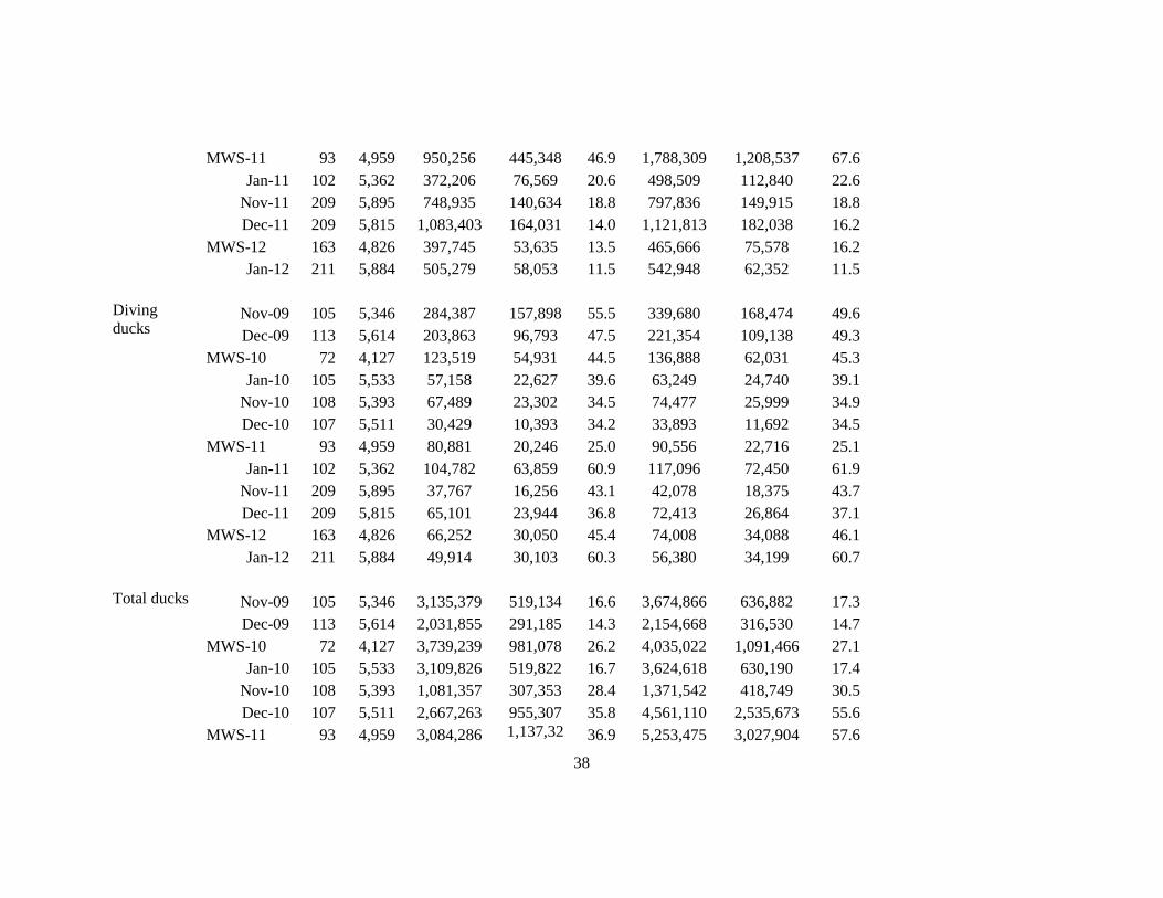
Table 6. Population estimates using uncorrected and detection probability-corrected values in the Arkansas portion of the Mississippi
Alluvial Valley for surveys conducted during winter 2009 to 2011. n = number of transects, km = total length of transects sampled, N
= estimated population.
Index Detection-adjusted Group Survey n km N SE %CV N SE %CV Mallards Nov-09 105 5,346 300,203 82,282 27.4 369,105 99,482 27.0
Dec-09 113 5,614 648,955 116,841 18.0 696,682 124,236 17.8
MWS-10 72 4,127 2,910,008 691,646 23.8 3,114,686 752,670 24.2
Jan-10 105 5,533 2,020,035 366,163 18.1 2,371,523 440,770 18.6
Nov-10 108 5,393 348,112 119,977 34.5 517,354 225,874 43.7
Dec-10 107 5,511 1,751,379 705,130 40.3 3,153,380 1,902,844 60.3
MWS-11 93 4,959 2,056,286 705,480 34.3 3,378,105 1,826,886 54.1
Jan-11 102 5,362 1,307,665 187,867 14.4 1,557,018 255,609 16.4
Nov-11 209 5,895 347,690 86,126 24.8 384,709 93,383 24.3
Dec-11 209 5,815 1,414,398 238,165 16.8 1,651,749 276,848 16.8
MWS-12 163 4,826 882,415 117,504 13.3 1,092,697 214,831 19.7
Jan-12 211 5,884 711,592 103,981 14.6 781,389 116,824 15.0
Other dabbling ducks
Nov-09 105 5,346 2,550,790 431,037 16.9 2,966,082 520,326 17.5 Dec-09 113 5,614 1,179,037 192,012 16.3 1,236,632 198,882 16.1
MWS-10 72 4,127 705,711 305,680 43.3 783,448 347,085 44.3
Jan-10 105 5,533 1,032,634 164,525 15.9 1,189,846 198,690 16.7
Nov-10 108 5,393 665,756 216,355 32.5 779,712 250,241 32.1
Dec-10 107 5,511 891,151 288,181 32.3 1,380,309 653,453 47.3
38
MWS-11 93 4,959 950,256 445,348 46.9 1,788,309 1,208,537 67.6
Jan-11 102 5,362 372,206 76,569 20.6 498,509 112,840 22.6
Nov-11 209 5,895 748,935 140,634 18.8 797,836 149,915 18.8
Dec-11 209 5,815 1,083,403 164,031 14.0 1,121,813 182,038 16.2
MWS-12 163 4,826 397,745 53,635 13.5 465,666 75,578 16.2
Jan-12 211 5,884 505,279 58,053 11.5 542,948 62,352 11.5
Diving ducks
Nov-09 105 5,346 284,387 157,898 55.5 339,680 168,474 49.6 Dec-09 113 5,614 203,863 96,793 47.5 221,354 109,138 49.3
MWS-10 72 4,127 123,519 54,931 44.5 136,888 62,031 45.3
Jan-10 105 5,533 57,158 22,627 39.6 63,249 24,740 39.1
Nov-10 108 5,393 67,489 23,302 34.5 74,477 25,999 34.9
Dec-10 107 5,511 30,429 10,393 34.2 33,893 11,692 34.5
MWS-11 93 4,959 80,881 20,246 25.0 90,556 22,716 25.1
Jan-11 102 5,362 104,782 63,859 60.9 117,096 72,450 61.9
Nov-11 209 5,895 37,767 16,256 43.1 42,078 18,375 43.7
Dec-11 209 5,815 65,101 23,944 36.8 72,413 26,864 37.1
MWS-12 163 4,826 66,252 30,050 45.4 74,008 34,088 46.1
Jan-12 211 5,884 49,914 30,103 60.3 56,380 34,199 60.7
Total ducks Nov-09 105 5,346 3,135,379 519,134 16.6 3,674,866 636,882 17.3 Dec-09 113 5,614 2,031,855 291,185 14.3 2,154,668 316,530 14.7
MWS-10 72 4,127 3,739,239 981,078 26.2 4,035,022 1,091,466 27.1
Jan-10 105 5,533 3,109,826 519,822 16.7 3,624,618 630,190 17.4
Nov-10 108 5,393 1,081,357 307,353 28.4 1,371,542 418,749 30.5
Dec-10 107 5,511 2,667,263 955,307 35.8 4,561,110 2,535,673 55.6
MWS-11 93 4,959 3,084,286 1,137,32
36.9 5,253,475 3,027,904 57.6

39
Jan-11 102 5,362 1,784,654 229,155 12.8 2,172,622 330,235 15.2
Nov-11 209 5,895 1,134,800 190,231 16.8 1,225,086 202,865 16.6
Dec-11 209 5,815 2,497,801 341,996 15.1 2,845,975 396,372 13.9
MWS-12 163 4,826 1,346,412 162,324 12.1 1,632,370 283,329 17.4
Jan-12 211 5,884 1,266,785 151,513 12.0 1,380,717 168,449 12.2

40
Table 7. Model selection results predicting waterfowl abundance for wintering waterfowl in the
Arkansas portion of the Mississippi Alluvial Valley during surveys conducted during winters
2009 to 2011. WSI.MAV is winter severity index for the MAV, WSI.DIFF, if the difference in
WSI between the MAV and mid-latitude locations to the north (latitude ~38 to 39). Model results
are ranked by Akaike’s Information Criterion adjusted for small sample size (AICc) value, delta
AICc (Δ AICc), and AICc weight (wi)
Taxon Model K AICc Δ AICc wi Mallards WSI.MAV 3 366.81 0.00 0.88
NULL 2 373.13 6.32 0.04
Other dabbling ducks NULL 2 365.59 0.39 0.60
Divers Year 4 307.01 0.00 0.41
WSI.MAV +WSI.DIFF+ Year + Month 8 308.12 1.11 0.24
Year + Month 6 308.82 1.81 0.17
NULL 2 310.33 3.32 0.08
All ducks WSI.MAV 3 377.07 0.00 0.48
NULL 2 377.56 0.49 0.38
41
Figure 1. Expert-opinion-based stratified sampling design for aerial waterfowl surveys in the
Arkansas portion of the Mississippi Alluvial Valley. Major rivers were used as guides in
determining strata boundaries and are shown for reference.

42
Figure 2. Watershed-based stratified sampling design for aerial waterfowl surveys in the
Arkansas portion of the Mississippi Alluvial Valley. Watersheds at the accounting unit level
(thick black line) and cataloguing unit level (thin black line) are shown for reference.

43
Figure 3. Watershed-based stratified sampling design for aerial waterfowl surveys in the
Louisiana portion of the Mississippi Alluvial Valley. Watersheds (thick black line) and sub-
watersheds (thin black line) boundaries are shown for reference.
44
Figure 4. Estimates of %CV of mean number of mallards and all ducks per transect in the
Arkansas portion of the Mississippi Alluvial Valley during surveys conducted during winters
2009-2010 to 2011-2012 winters. Dotted line shows target precision of 15% CV.

45
Figure 5. Population indices compared to detection-adjusted numbers of mallards in the
Arkansas portion of the Lower Mississippi Alluvial Valley during winters 2009-2010 to 2011-
2012 with 95% confidence intervals from bootstrapping. MWS=midwinter survey, conducted in
early January of each year.

46
Figure 6. Population indices compared to detection-adjusted numbers of all dabbling ducks other
than mallards in the Arkansas portion of the Lower Mississippi Alluvial Valley during winters
2009-2010 to 2011-2012 with 95% confidence intervals from bootstrapping. MWS=midwinter
survey, conducted in early January of each year.

47
Figure 7. Population indices compared to detection-adjusted numbers of diving ducks in the
Arkansas portion of the Lower Mississippi Alluvial Valley during winters 2009-2010 to 2011-
2012 with 95% confidence intervals from bootstrapping. MWS=midwinter survey, conducted in
early January of each year.

48
Figure 8. Population indices compared to detection-adjusted numbers of all ducks in the
Arkansas portion of the Lower Mississippi Alluvial Valley during winters 2009-2010 to 2011-
2012 with 95% confidence intervals from bootstrapping. MWS=midwinter survey, conducted in
early January of each year.

49
Figure 9. Number of mallards in the Arkansas portion of the Mississippi Alluvial Valley as
predicted by the Winter Severity Index (see methods) in the region during winters 2009-2011.
Dotted lines indicate 95% confidence intervals. Higher values indicate more severe weather
conditions, points indicate observed values.
50
Appendix A. Use of public lands by waterfowl according to habitat type.

Appendix A1. Detection-bias corrected mallard use by land ownership and habitat. Use relative to availability is % Use divided by % available by survey. Habitat codes: Ag=non-rice agriculture, bay=bayou, blh=bottomland hardwood, cyp-tup= cypress-tupelo, fish-res= aquaculture impoundments and reservoirs, msu=moist-soil, ox=oxbow lakes, ss=shrub-scrub.
Survey Land % Use Use rel. to avail.
Pop. Est. for AR MAV ag bay blh
cyp-tup
ditch
fishres lake msu ox rice river ss
Nov 2009 Federal 15% 3.51 35,112 0 0 0 49 0 0 0 0 0 51 0 0 Nov 2009 Private 85% 0.91 317,135 64 0 0 0 0 1 0 10 6 20 0 0 Nov 2009 State 0% 0.00 - 0 0 0 0 0 0 0 0 0 0 0 0 Nov 2009 All 100% 1.00 369,105 54 0 0 8 0 1 0 9 5 24 0 0 Dec 2009 Federal 7% 1.98 37,418 5 1 10 0 0 0 0 78 0 0 0 6 Dec 2009 Private 89% 0.95 620,310 40 0 7 0 0 20 0 14 0 16 0 3 Dec 2009 State 4% 1.57 27,132 72 0 0 2 0 0 0 11 0 15 0 0 Dec 2009 All 100% 1.00 696,682 39 0 7 0 0 18 0 18 0 15 0 3 MWS 2010 Federal 4% 0.76 63,971 42 0 23 0 0 0 12 0 1 22 0 1 MWS 2010 Private 92% 1.02 2,979,624 25 0 3 0 0 38 0 25 1 5 0 4 MWS 2010 State 4% 0.96 73,972 14 0 13 0 0 51 0 23 0 0 0 0 MWS 2010 All 100% 1.00 3,114,686 25 0 4 0 0 37 1 24 1 5 0 3 Jan 2010 Federal 4% 0.93 59,942 20 19 14 0 0 0 37 8 0 1 1 1 Jan 2010 Private 91% 0.99 2,202,011 61 0 0 0 0 2 0 11 1 25 0 1 Jan 2010 State 5% 1.46 85,921 3 0 1 88 0 0 0 4 4 0 0 0 Jan 2010 All 100% 1.00 2,371,523 56 1 1 4 0 1 1 10 1 23 0 1 Nov 2010 Federal 17% 4.88 68,456 0 0 0 96 0 0 0 0 3 0 0 1 Nov 2010 Private 83% 0.88 429,058 10 0 0 30 0 18 0 2 0 37 1 2 Nov 2010 State 0% 0.11 1,387 0 0 0 0 0 0 0 0 29 0 71 0 Nov 2010 All 100% 1.00 517,354 8 0 0 41 0 15 0 2 1 30 1 2 Dec 2010 Federal 47% 10.37 886,370 0 0 0 83 0 2 0 0 0 12 2 0 Dec 2010 Private 49% 0.54 1,596,415 11 1 3 6 0 35 12 3 0 13 4 13 Dec 2010 State 4% 1.01 79,141 1 1 2 0 0 0 85 2 0 0 8 0 Dec 2010 All 100% 1.00 3,153,380 5 0 2 42 0 18 9 1 0 12 4 6 Mid 2011 Federal 5% 1.31 119,477 3 0 1 0 0 1 0 1 91 0 2 2

52
Mid 2011 Private 66% 0.72 2,273,051 25 0 1 2 0 23 0 7 1 40 1 1 Mid 2011 State 29% 7.62 638,159 0 0 0 100 0 0 0 0 0 0 0 0 Mid 2011 All 100% 1.00 3,378,105 17 0 1 30 0 15 0 4 5 27 0 1 Jan 2011 Federal 6% 1.61 67,906 7 0 1 65 0 0 0 0 19 5 1 3 Jan 2011 Private 94% 1.00 1,464,765 18 1 0 1 2 4 0 12 0 51 0 11 Jan 2011 State 1% 0.01 454 3 7 10 47 0 0 0 1 12 0 0 20 Jan 2011 All 100% 1.00 1,557,018 17 1 1 5 1 4 0 12 1 48 0 11 Nov 2011 Federal 12% 3.45 35,977 0 0 0 0 4 0 89 0 0 7 0 0 Nov 2011 Private 88% 0.94 341,421 28 0 1 1 1 0 2 0 19 48 0 0 Nov 2011 State 0% 0.00 - 0 0 0 0 0 0 0 0 0 0 0 0 Nov 2011 All 100% 1.00 384,709 25 0 1 1 0 17 0 13 0 43 0 0 Dec 2011 Federal 13% 3.25 145,483 20 0 1 40 40 0 0 39 0 0 0 0 Dec 2011 Private 84% 0.90 1,403,570 27 0 1 3 3 23 0 17 1 25 0 0 Dec 2011 State 3% 0.98 40,080 1 0 29 0 0 70 0 0 0 0 0 0 Dec 2011 All 100% 1.00 1,651,749 25 0 2 8 0 21 0 20 0 21 0 0 MWS 2012 Federal 17% 3.49 103,404 2 0 5 43 0 0 0 49 0 0 0 0 MWS 2012 Private 83% 0.90 920,997 35 0 1 0 0 8 0 10 1 39 0 6 MWS 2012 State 0% 0.07 2,014 10 0 80 0 0 0 0 6 0 0 0 5 MWS 2012 All 100% 1.00 1,092,697 30 0 2 7 0 7 0 16 1 32 0 5 Jan 2012 Federal 11% 3.14 66,595 19 1 22 0 0 0 0 25 0 0 12 0 Jan 2012 Private 86% 0.92 675,428 30 0 2 0 1 5 0 30 1 29 0 1 Jan 2012 State 3% 0.96 18,625 1 0 4 0 0 0 0 51 0 38 2 2 Jan 2012 All 100% 1.00 781,389 28 0 4 0 0 4 0 30 0 26 1 1 Ave Federal 13% 3.22 140,843 10 2 6 31 4 0 11 17 9 8 1 1 Ave Private 82% 0.89 1,268,649 31 0 2 4 1 15 1 12 2 29 1 4 Ave State 4% 1.23 80,574 10 1 14 24 0 12 9 10 4 5 8 3 Ave All 100% 1.00 1,589,033 27 0 2 12 0 13 1 13 1 26 1 3

53
Appendix A2. Detection-bias corrected mallard use by land ownership and habitat. Use relative to availability is % Use divided by % available by survey. Habitat codes: Ag=non-rice agriculture, bay=bayou, blh=bottomland hardwood, cyp-tup= cypress-tupelo, fish-res= aquaculture impoundments and reservoirs, msu=moist-soil, ox=oxbow lakes, ss=shrub-scrub.
Survey Land % Use Use rel. to avail.
Pop. Est. for AR MAV
ag bay blh cyp-tup ditch fish
res lake msu ox rice river ss
Nov 2009 Federal 20.5% 4.7 380,540 48 0 0 30 0 0 0 4 0 18 0 0 Nov 2009 Private 75.3% 0.8 2,262,963 64 0 0 0 0 2 0 16 2 15 0 0 Nov 2009 State 4.3% 1.5 113,101 8 0 5 2 0 2 0 84 0 0 0 0 Nov 2009 All
2,966,082 58 0 0 7 0 2 0 17 2 15 0 0
Dec 2009 Federal 0.5% 0.0 168 65 0 9 0 0 0 0 26 0 0 0 0 Dec 2009 Private 97.4% 1.0 1,133,415 73 0 0 0 0 9 0 6 2 10 0 1 Dec 2009 State 2.1% 0.0 644 35 0 0 0 0 2 0 44 2 18 0 0 Dec 2009 All
1,236,632 72 0 0 0 0 8 0 7 2 10 0 1
MWS 2010 Federal 2.9% 0.5 11,110 22 0 8 0 2 0 4 0 0 65 0 0 MWS 2010 Private 95.8% 1.1 779,584 26 0 0 0 0 10 0 56 0 8 0 0 MWS 2010 State 1.2% 0.3 6,034 89 0 2 0 0 9 0 0 0 0 0 0 MWS 2010 All
783,448 27 0 0 0 0 9 0 54 0 9 0 0
Jan 2010 Federal 2.1% 0.5 15,789 51 0 0 0 0 0 2 47 0 0 0 0 Jan 2010 Private 93.4% 1.0 1,131,448 67 0 1 0 0 1 0 7 0 23 0 1 Jan 2010 State 4.5% 1.4 40,414 15 0 0 81 0 0 0 3 1 0 0 0 Jan 2010 All
1,189,846 64 0 1 4 0 1 0 7 0 22 0 1
Nov 2010 Federal 0.5% 0.1 3,017 0 2 0 15 0 0 0 0 66 0 0 18 Nov 2010 Private 99.1% 1.1 775,812 12 0 0 11 0 57 1 4 3 12 0 1 Nov 2010 State 0.4% 0.1 2,786 0 0 0 0 0 96 0 0 4 0 0 0 Nov 2010 All
779,712 12 0 0 11 0 57 1 3 4 11 0 1
Dec 2010 Federal 32% 7.1 263,896 0 0 0 76 0 0 0 0 0 24 0 0

54
Dec 2010 Private 66% 0.7 935,019 12 1 0 5 1 26 34 1 0 14 1 5 Dec 2010 State 2% 0.5 18,725 6 0 0 0 0 0 63 0 0 0 31 0 Dec 2010 All
1,380,309 8 0 0 28 0 17 24 1 0 17 1 4
Mid 2011 Federal 0.6% 0.2 8,433 0 1 0 2 0 95 0 0 0 0 0 2 Mid 2011 Private 51.0% 0.6 925,625 17 0 0 1 0 36 4 4 1 40 0 1 Mid 2011 State 48.5% 12.7 561,122 0 0 0 83 0 16 0 0 1 0 0 0 Mid 2011 All
1,788,309 9 0 0 40 0 27 0 2 1 20 0 1
Jan 2011 Federal 7.3% 2.1 28,857 2 0 0 97 1 0 0 0 0 0 0 0 Jan 2011 Private 89.4% 1.0 448,408 12 0 0 5 0 18 0 7 0 55 0 3 Jan 2011 State 3.3% 0.0 436 0 0 0 45 0 0 0 4 0 0 0 51 Jan 2011 All
498508.82 11 0 0 13 0 16 0 6 0 49 0 4
Nov 2011 Federal 8.5% 2.4 78,333 96 0 0 0 0 0 1 0 0 2 0 0 Nov 2011 Private 91.4% 1.0 1,090,031 27 0 0 1 3 0 2 2 18 44 0 2
Nov 2011 State 0.1% 0.0 912 0 0 0 0 0 0 0 0 100 0 0 0
Nov 2011 All
1,182,545 33 0 0 2 0 17 0 2 2 41 0 2 Dec 2011 Federal 10.9% 2.7 200,208 35 0 0 20 0 0 0 40 6 0 0 0 Dec 2011 Private 87.1% 0.9 2,435,109 37 0 0 1 0 14 0 7 0 40 0 0 Dec 2011 State 2.0% 0.8 53,841 11 0 0 0 0 88 0 1 0 0 0 0 Dec 2011 All
2,773,562 36 0 0 3 0 14 0 10 1 35 0 0
MWS 2012 Federal 13.6% 2.8 35,254 14 1 0 52 0 0 0 48 0 0 0 0 MWS 2012 Private 86.3% 0.9 409,085 86 0 0 0 0 18 0 13 3 25 0 0
MWS 2012 State 0.0% 0.0 - 0 0 0 0 0 0 0 0 100 0 0 0
MWS 2012 All
465,666 34 0 0 7 0 15 0 17 3 22 0 0 Jan 2012 Federal 7.6% 2.1 31,122 41 0 0 1 1 0 0 49 0 0 4 0 Jan 2012 Private 91.0% 1.0 499,511 38 0 0 0 0 17 0 21 0 24 0 0

55
Jan 2012 State 1.4% 0.4 5,662 0 0 0 0 0 2 0 65 0 33 0 0 Jan 2012 All
542,948 37 0 0 0 0 15 0 23 0 23 0 0
Ave Federal 8.9% 2.1 88,060 31 0 2 24 0 8 1 18 6 9 0 2 Ave Private 85.3% 0.9 1,068,834 39 0 0 2 0 17 3 12 3 26 0 1 Ave State 5.8% 1.5 66,973 14 0 1 18 0 18 5 17 17 4 3 4 Ave All 1,298,964 33 0 0 10 0 16 2 12 1 23 0 1

56
Appendix A3. Detection-bias corrected mallard use by land ownership and habitat. Use relative to availability is % Use divided by % available by survey. Habitat codes: Ag=non-rice agriculture, bay=bayou, blh=bottomland hardwood, cyp-tup= cypress-tupelo, fish-res= aquaculture impoundments and reservoirs, msu=moist-soil, ox=oxbow lakes, ss=shrub-scrub.
Survey Land % Use Use
rel. to avail.
Pop. Est. for AR MAV
ag bay blh cyp-tup ditch fish
res lake msu ox rice river ss
Nov 2009 Federal 57% 13.2 121,173 73 0 0 26 0 0 0 0 0 0 0 0 Nov 2009 Private 41% 0.4 140,764 77 0 0 0 0 3 0 20 0 0 0 0 Nov 2009 State 2% 0.8 6,326 0 0 0 0 0 0 0 100 0 0 0 0 Nov 2009 All 100% 1.0 339,680 73 0 0 15 0 1 0 10 0 0 0 0 Dec 2009 Federal 0% 0.0 - 0 0 0 0 0 0 0 0 0 0 0 0 Dec 2009 Private 100% 1.1 222,197 3 0 0 3 0 90 0 0 4 0 0 0 Dec 2009 State 0% 0.0 - 0 0 0 0 0 0 0 0 0 0 0 0 Dec 2009 All 100% 1.0 221,354 3 0 0 3 0 90 0 0 4 0 0 0 MWS 2010 Federal 0% 0.0 - 0 0 0 0 0 0 0 0 0 0 0 0 MWS 2010 Private 100% 1.1 142,185 3 0 0 0 3 33 0 27 34 0 0 0 MWS 2010 State 0% 0.0 - 0 0 0 0 0 0 0 0 0 0 0 0 MWS 2010 All 100% 1.0 136,888 3 0 0 0 3 33 0 27 33 0 0 0 Jan 2010 Federal 0% 0.0 - 0 0 0 0 0 0 0 0 0 0 0 0 Jan 2010 Private 98% 1.1 63,364 14 0 0 0 0 65 0 15 0 0 4 2 Jan 2010 State 2% 0.5 764 0 0 0 0 0 0 0 100 0 0 0 0 Jan 2010 All 100% 1.0 63,249 14 0 0 0 0 64 0 16 0 0 4 1 Nov 2010 Federal 0% 0.0 - 0 0 0 0 0 0 0 0 0 0 0 0 Nov 2010 Private 100% 1.1 74,777 0 0 0 0 0 100 0 0 0 0 0 0 Nov 2010 State 0% 0.0 - 0 0 0 0 0 0 0 0 0 0 0 0 Nov 2010 All 100% 1.0 74,477 0 0 0 0 0 100 0 0 0 0 0 0 Dec 2010 Federal 0% 0.0 - 0 0 0 0 0 0 0 0 0 0 0 0

57
Dec 2010 Private 100% 1.1 34,734 0 0 0 0 0 98 0 0 0 0 2 0 Dec 2010 State 0% 0.0 - 0 0 0 0 0 0 0 0 0 0 0 0 Dec 2010 All 100% 1.0 33,893 0 0 0 0 0 98 0 0 0 0 2 0 Mid 2011 Federal 16% 4.7 11,601 0 0 0 0 0 96 0 4 4 0 0 0 Mid 2011 Private 75% 0.8 69,205 2 0 0 0 0 89 1 2 2 1 1 4 Mid 2011 State 8% 2.2 4,921 0 0 0 0 0 100 0 0 0 0 0 0 Mid 2011 All 100% 1.0 90,556 2 0 0 0 0 91 0 1 2 0 1 3 Jan 2011 Federal 0% 0.0 - 0 0 0 0 0 0 0 0 0 0 0 0 Jan 2011 Private 100% 1.1 117,698 0 0 0 0 0 76 0 0 19 5 0 0 Jan 2011 State 0% 0.0 3 0 0 0 0 0 0 0 0 100 0 0 0 Jan 2011 All 100% 1.0 117,096 0 0 0 0 0 76 0 0 19 5 0 0 Nov 2011 Federal 0% 0.0 - 0 0 0 0 0 0 0 0 0 0 0 0 Nov 2011 Private 100% 1.1 42,436 0 3 0 0 0 89 1 0 0 0 1 6 Nov 2011 State 0% 0.0 - 0 0 0 0 0 0 0 0 0 0 0 0 Nov 2011 All 100% 1.0 42,078 0 3 0 0 0 89 1 0 0 0 1 6 Dec 2011 Federal 0% 0.0 - 0 0 0 0 0 0 0 0 0 0 0 0 Dec 2011 Private 92% 1.0 67,080 20 0 0 0 0 4 0 0 74 1 0 0 Dec 2011 State 8% 3.2 5,693 0 0 0 0 0 0 0 0 100 0 0 0 Dec 2011 All 100% 1.0 72,413 18 0 0 0 4 76 0 4 0 1 0 0 MWS 2012 Federal 1% 0.1 288 0 0 0 0 0 0 0 0 100 0 0 0 MWS 2012 Private 92% 1.0 69,535 8 0 0 0 0 71 1 12 0 0 0 0 MWS 2012 State 7% 2.6 4,774 0 0 0 0 0 100 0 0 0 0 0 0 MWS 2012 All 100% 1.0 74,008 8 0 0 0 0 72 0 11 1 0 0 0 Jan 2012 Federal 0% 0.0 - 0 0 0 0 0 0 0 0 0 0 0 0 Jan 2012 Private 99% 1.1 56,600 6 0 0 0 0 93 0 0 1 0 0 0 Jan 2012 State 1% 0.2 294 0 0 0 0 0 100 0 0 0 0 0 0 Jan 2012 All 100% 1.0 56,380 6 0 0 0 0 93 0 0 1 0 0 0

58
Ave Federal 6% 1.5 4,487 24 0 0 9 0 32 0 1 35 0 0 0 Ave Private 92% 1.0 102,233 11 0 0 0 0 68 0 6 11 1 1 1 Ave State 2% 0.8 2,143 0 0 0 0 0 43 0 29 29 0 0 0 Ave All 100% 1.0 110,173 11 0 0 2 1 74 0 6 5 1 0 1

59
Appendix A4. Detection-bias corrected mallard use by land ownership and habitat. Use relative to availability is % Use divided by % available by survey. Habitat codes: Ag=non-rice agriculture, bay=bayou, blh=bottomland hardwood, cyp-tup= cypress-tupelo, fish-res= aquaculture impoundments and reservoirs, msu=moist-soil, ox=oxbow lakes, ss=shrub-scrub.
Survey Land % Use
Use rel. to avail.
Pop. Est. for AR MAV
ag bay blh cyp-tup ditch fish
res lake msu ox rice river ss
Nov 2009 Federal 23% 5.3 526,672 50 0 0 31 0 0 0 3 0 17 0 0 Nov 2009 Private 73% 0.8 2,732,983 65 0 0 0 0 2 0 16 2 15 0 0 Nov 2009 State 4% 1.3 120,575 7 0 4 2 0 1 0 85 0 0 0 0 Nov 2009 All 100% 1.0 3,674,866 59 0 0 7 2 2 0 16 2 15 0 0 Dec 2009 Federal 3% 0.8 45,638 11 1 10 0 0 0 0 72 0 0 0 6 Dec 2009 Private 95% 1.0 2,046,078 55 0 2 1 0 21 0 8 2 11 0 2 Dec 2009 State 3% 1.0 51,947 55 0 0 1 0 1 0 26 1 16 0 0 Dec 2009 All 100% 1.0 2,154,668 54 0 2 1 0 20 0 10 1 10 0 2 MWS 2010 Federal 4% 0.7 76,954 40 0 21 0 0 0 11 0 1 27 0 1 MWS 2010 Private 93% 1.0 3,893,580 24 0 2 0 0 33 0 30 2 5 0 3 MWS 2010 State 3% 0.8 82,879 18 0 12 0 0 48 0 21 0 0 0 0 MWS 2010 All 100% 1.0 4,035,022 25 0 3 0 0 32 1 29 1 6 0 3 Jan 2010 Federal 3% 0.8 75,582 27 15 11 0 0 0 29 17 0 1 1 1 Jan 2010 Private 92% 1.0 3,398,749 62 0 0 0 0 3 0 10 1 24 0 1 Jan 2010 State 5% 1.4 125,849 7 0 1 85 0 0 0 4 3 0 0 0 Jan 2010 All 100% 1.0 3,624,618 58 1 1 4 0 3 1 9 1 22 0 1 Nov 2010 Federal 7% 2.0 73,230 0 0 0 93 0 0 0 0 6 0 0 1 Nov 2010 Private 93% 1.0 1,277,927 10 0 0 17 0 46 0 3 2 20 0 1 Nov 2010 State 0% 0.1 3,676 0 0 0 0 0 60 0 0 13 0 27 0 Nov 2010 All 100% 1.0 1,371,542 10 0 0 22 0 43 0 0 3 18 0 1 Dec 2010 Federal 41% 9.1 1,128,981 0 0 0 81 0 2 0 0 0 15 2 0

60
Dec 2010 Private 56% 0.6 2,603,563 11 1 2 5 0 33 20 2 0 13 3 10 Dec 2010 State 3% 0.8 95,908 2 1 2 0 0 0 81 1 0 0 13 0 Dec 2010 All 100% 1.0 4,561,110 6 0 1 36 0 19 14 1 0 14 3 5 Mid 2011 Federal 4% 1.0 148,645 3 0 1 0 0 18 0 1 75 0 1 1 Mid 2011 Private 62% 0.7 3,289,686 22 0 1 1 0 28 0 6 1 39 1 2 Mid 2011 State 35% 9.1 1,182,767 0 0 0 92 0 8 0 0 14 4 1 2 Mid 2011 All 100% 1.0 5,253,475 14 0 0 33 0 21 0 3 4 24 0 1 Jan 2011 Federal 6% 1.7 98,199 5 0 1 73 0 0 0 11 1 51 0 9 Jan 2011 Private 93% 1.0 2,028,593 16 1 0 1 1 9 0 2 7 0 0 34 Jan 2011 State 2% 0.0 864 2 4 6 46 0 0 0 4 14 0 0 25 Jan 2011 All 100% 1.0 2,172,622 15 1 0 6 1 8 0 10 1 47 0 9 Nov 2011 Federal 9% 2.7 89,743 56 0 0 0 2 0 38 0 0 4 0 0 Nov 2011 Private 91% 1.0 1,118,124 27 0 0 1 2 0 2 2 21 44 0 1 Nov 2011 State 0% 0.0 - 0 0 0 0 0 0 0 0 100 0 0 0 Nov 2011 All 100% 1.0 1,225,086 29 0 0 2 0 19 0 5 1 40 0 1 Dec 2011 Federal 12% 3.0 228,052 25 0 1 33 0 0 0 40 2 0 0 0 Dec 2011 Private 86% 0.9 2,452,786 31 0 1 2 0 21 0 13 0 30 0 0 Dec 2011 State 2% 0.9 66,296 4 0 18 0 0 78 0 0 0 0 0 0 Dec 2011 All 100% 1.0 2,845,975 29 0 1 6 0 19 0 16 1 26 0 0 MWS 2012 Federal 16% 3.2 143,570 2 0 4 45 0 0 0 49 0 0 0 0 MWS 2012 Private 84% 0.9 1,392,487 36 0 1 0 0 12 0 10 1 35 0 5 MWS 2012 State 0% 0.1 6,017 5 0 39 0 0 48 0 3 4 0 0 2 MWS 2012 All 100% 1.0 1,632,370 30 0 1 7 0 10 0 16 1 29 0 4 Jan 2012 Federal 10% 2.7 99,971 26 1 15 0 0 0 0 32 0 0 9 0 Jan 2012 Private 88% 0.9 1,228,381 33 0 1 0 0 12 0 25 0 27 0 1 Jan 2012 State 2% 0.7 24,682 1 0 3 0 0 1 0 54 0 37 1 2 Jan 2012 All 100% 1.0 1,380,717 31 0 2 0 0 11 0 27 0 24 1 1

61
Ave Federal 11% 2.7 227,936 20 1 5 30 0 2 6 19 7 9 1 2 Ave Private 84% 0.9 2,288,578 33 0 1 2 0 18 2 11 3 22 0 5 Ave State 5% 1.4 146,788 8 0 7 19 0 20 7 16 12 5 3 3 Ave All 100% 1.0 2,827,673 30 0 1 10 0 17 1 12 1 23 0 2

Appendix B. Screen shots of GUI.

63
Appendix B1. Screen shot of Main Menu of waterfowl GUI.

64
Appendix B2. Screen shot of “Create files for New Survey” in waterfowl GUI. Window asks the
location of the transects to be selected.

65
Appendix B3. Screen shot of “Create files for New Survey” in waterfowl GUI. User inputs
month and year and selects folder where files should be saved. If desired, user edits total desired
km in each strata. After “Generate and Save Transects” button is pressed, GUI outputs five text
files: four of these are for input into the “Record” program (or files to be read into GPS unit in
the case of Mississippi). A fifth file lists the target and actual total transect lengths in each strata.
A shapefile of the randomly selected transects is also saved.

66
Appendix B4. Screen shot of main analysis window in waterfowl GUI.

67
Appendix B5. Screen shot of “Check Column Names” window under the analysis option in the
waterfowl GUI. For analysis, the GUI requires eight (8) columns: observer, stratum, transect, X,
Y, species, count, and habitat. Because these columns must be named exactly as shown, this
window allows the user to edit the column names.

68
Appendix B6. Screen shot of “Check Count Error” window under the analysis option in the
waterfowl GUI. This window displays any non-numeric text that has been entered in the “count”
column along with the species, habitat, and file in which the text was located. This allows the
user to correct any typos that were inadvertently entered into the data.

69
Appendix B7. Screen shot of “Create New Group” window under the analysis option in the
waterfowl GUI. This window allows the user to create new groups (e.g. all ducks combined) to
be used in the analysis. The user inputs a “1” next to the species to be included in the group and
then enters a name for the group.

70
Appendix B8. Screen shot of “Kernel Density Estimates” window under the analysis option in
the waterfowl GUI. This window allows the user to create kernel density estimates for any
species or previously created group. The user inputs coordinate type (lat-long or UTM) and
smoothing factor (default is 16 km) and selects species or group from pull-down list. Pressing
“Generate Kernel” creates the kernel and displays it overlaid a map of the United States.
Individual locations are displayed as points. Selecting “Save Kernel” saves a tiff file that can
then be imported into a GIS (e.g. ArcGIS).

71
Appendix B9. Screen shot of “Detection Correction Factor” window under the analysis option in
the waterfowl GUI. This window allows the user to adjust for detection bias by observer and
canopy cover. The default values were calculated using data collected in the Arkansas MAV
during February of 2012. Because these values are observer specific, they should not be used
outside of surveys flown by these same observers. The user specifies which habitat types quality
as closed canopy by entering a “1” in the “Closed” column.

72
Appendix B10. Screen shot of main analysis window in the waterfowl GUI. After the user has
inspected and cleaned the data, the user can generate estimates of species and total duck
numbers. After inputting the month and year (used in naming the output files) and selecting a
folder for the generated files, the user selects “Analyze and Save Data Files”. The GUI then
generates estimates of species and total duck numbers by strata with SEs and bootstrapped 95%
confidence intervals. The GUI also summarizes habitat by % of each species observed in each
habitat type and provides a summary of the species observed by transect.