FINAL EXAM Spring 2011

TFY4235/FY8904 Computational Physics

This exam is published on Friday, May 13, 2011 at 09:00 hours. The solutions should be

mailed to me at Alex.Hansen@ntnu.no on Monday, May 16 at 23:00 hours at the latest.

There are no constraints on any aids you may want to use in connection with this exam,

including discussing it with anybody. Do collaborate on the development of the programs,

but write your own code. The final report you will have to write yourself.

Please attach your programs as appendices to the report. The report may be written in

either Norwegian (either variation) or in English. Please use name rather than candidate

number on the report.

The reports should be in PDF format and consist of a single file.

This year’s topic is line tension in the two-dimensional Ising model. We will test a

new numerical method for calculating this quantity.

The Ising model implemented on a square lattice has the Hamiltonian (energy func-

tion)

H = −J

2

∑

<~m,~n>

σ~mσ~n , (1)

where σ~m = ±1 is the spin at node ~m and the sum over < ~m,~n > runs over all nearest

neighbors. Hence, for each ~m, we sum over its four nearest neighbors ~n. This leads to

double counting, explaining the factor 1/2. The coupling strength is J . In the following,

we set J = 1.

We now describe the square lattice. We orient it with respect to a cartesian coordinate

system (x, y) so that the principal axes coincide with the axes of the coordinate system.

Hence, the node address ~m can be written ~m = (im, jm), where im is the coordinate of ~m

along the x axis and jm is the coordinate of ~m along the y axis. We limit the size of the

lattice to the two intervals 1 ≤ im ≤ Nx and 1 ≤ jm ≤ Ny.

We assume in the following periodic boundary conditions in the y direction. That is,

the lattice is rolled into a tube so that the jm = 1 and jm = Ny rows are next to each

other. We will in a moment discuss the boundary conditions in the x direction.

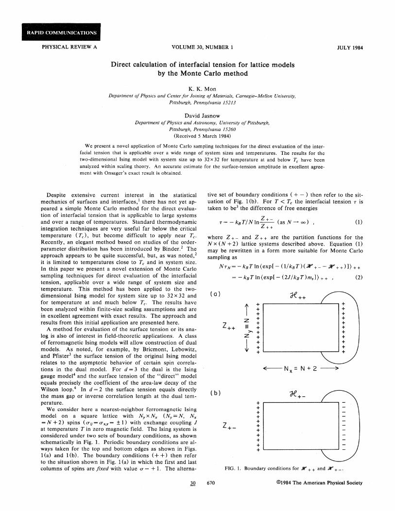
In 1984, Mon and Jasnow (Phys. Rev. A, 30, 670 (1984)) proposed an algorithm to

measure the line tension in the Ising model. The line tension is the free energy associated

1

with the boundaries between islands of up and down spins. Mon and Jasnow proposed the

follwing: Prepate two lattices as described above. In both of them, add a row in the y

direction with im = 0. Along this row, all spins are fixed (i.e., do not change) and set to the

value σ(0,j) = +1. Next, in one of the lattices add a row in the y direction at im = Nx + 1

where the spins are fixed, σ(Nx+1,j) = +1, whereas in the other lattice, the extra row in

(Nx + 1, j) has fixed spins with value σ(Nx+1,j) = −1. The hamiltonian, defined in Eq.

(1), for the first lattice we denote H++, whereas the hamiltonian for the second lattice, we

denote H+−.

We may now define the free energy associated with the line tension in the Ising model.

If F++ is the free energy associated with the ++ lattice and +− the free energy associated

with the +− lattice, the surface tension free energy iτ is

Nyτ = F+− − F++ . (2)

This is easy to understand intuitively since in the +− lattice there must be an interface

at zero temperature T forced into existence by the boundary conditions in the x direction.

The free energies F++ and F+− are related to the partition functions and hence the

hamiltonians through the expressions

e−F++/kBT = Z++ =∑

conf.

e−H++/kBT , (3)

and

e−F+−/kBT = Z+− =∑

conf.

e−H+−/kBT . (4)

The sum runs over all possible spin configurations. In the following, we use units so that

the Boltzmann constant kB = 1.

Combining Eq. (2) with Eqs. (3) and (4) gives

τ = − T

Nyln

Z+−

Z++. (5)

The ratio between the two partition functions may be written (and this is main ob-

servation of Mon and Jasnow)

Z+−

Z++=

∑

conf. e−(H+−−H++)/T e−H++/T

Z++= 〈e−(H+−−H++)/T 〉++ . (6)

That is, the ratio Z+−/Z++ equals average of the quantity exp[−(H+− −H++)/T ] in the

system governed by the H++ hamiltonian.

2

The quantity 〈exp[−(H+−−H++)/T ]〉++ we sample numerically using the Metropolis

Monte Carlo algorithm. That is, we use the Boltzmann weight exp[−H++/T ] for the

probability distribution.

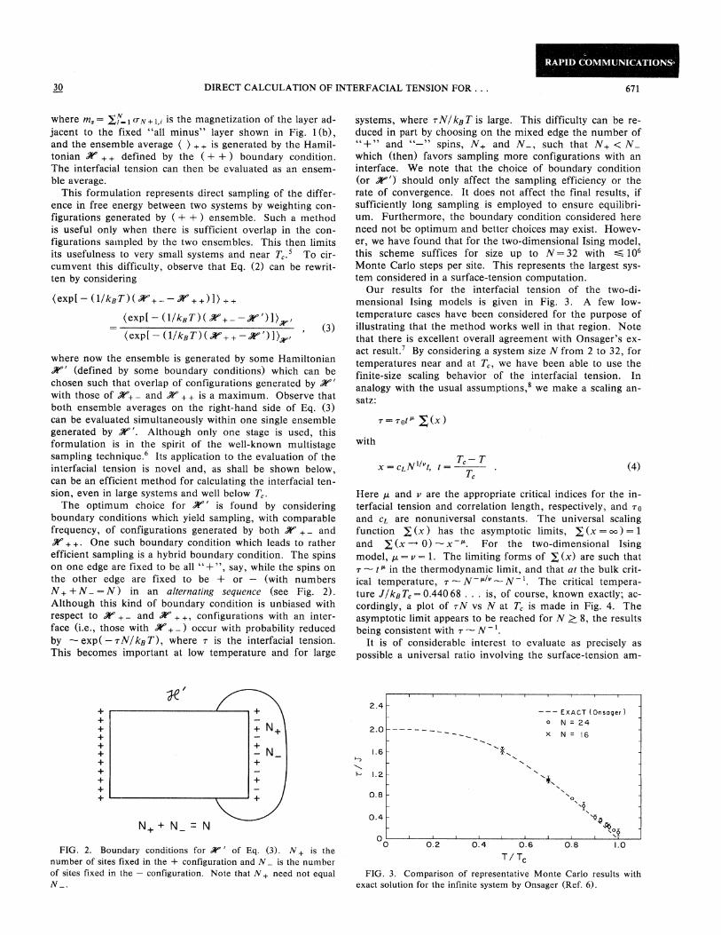
So far the Mon and Jasnow algorithm for calculating τ . Here is the new idea for

this exam. The Mon and Jasnow algoritm uses two fixed boundary layers at im = 0 and

im = Nx + 1. These two fixed boundary conditions will disturb the calculation for small

lattice sizes and getting rid of them would be an improvement. We therefore introduce

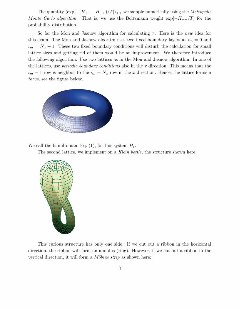
the following algorithm. Use two lattices as in the Mon and Jasnow algorithm. In one of

the lattices, use periodic boundary conditions also in the x direction. This means that the

im = 1 row is neighbor to the im = Nx row in the x direction. Hence, the lattice forms a

torus, see the figure below.

We call the hamiltonian, Eq. (1), for this system Ht.

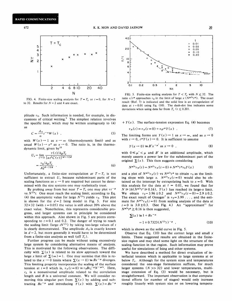
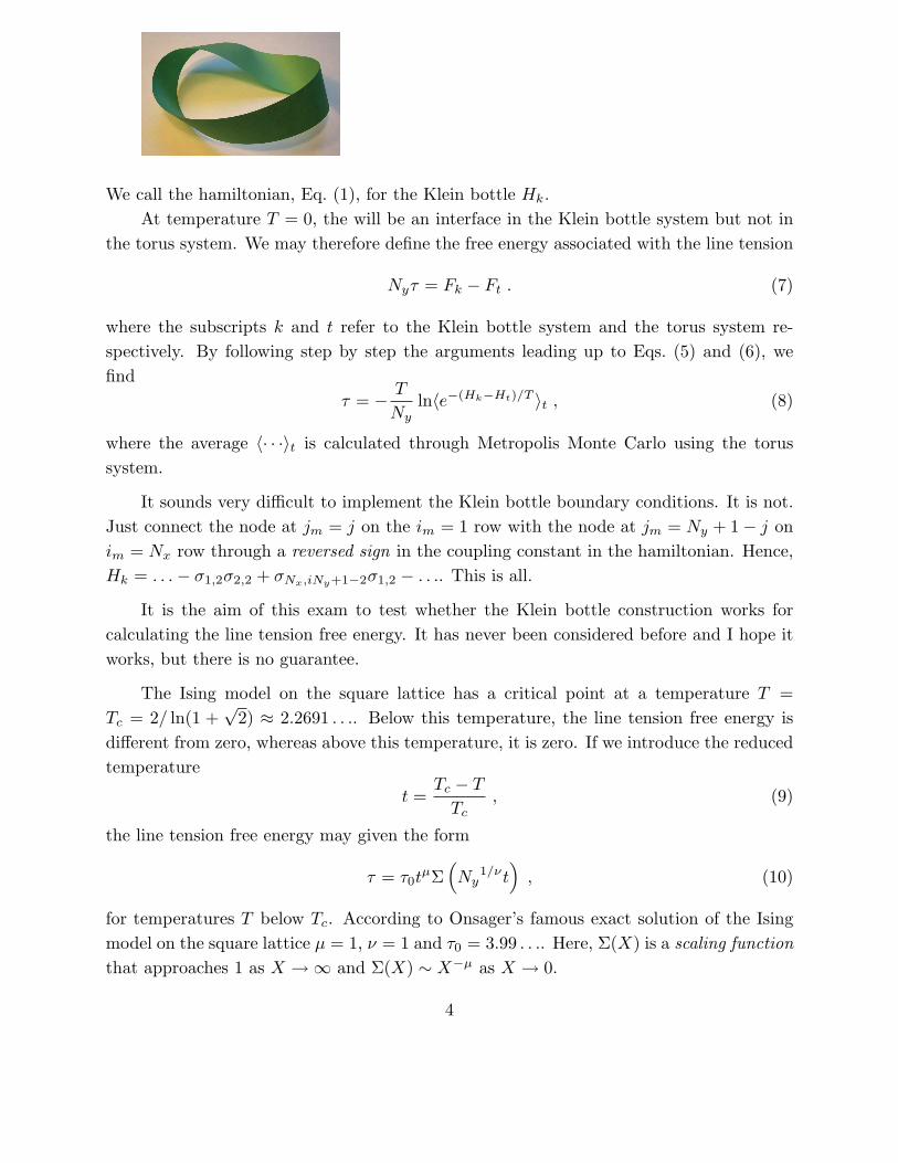
The second lattice, we implement on a Klein bottle, the structure shown here:

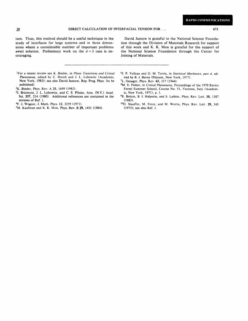
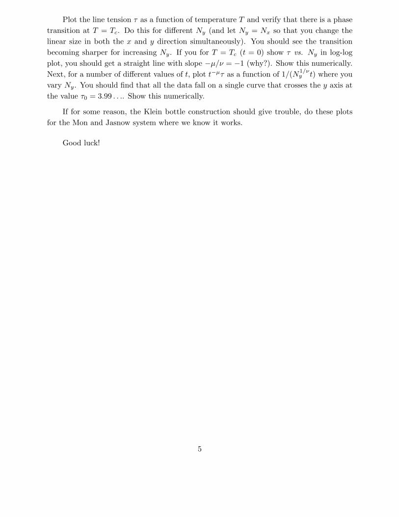
This curious structure has only one side. If we cut out a ribbon in the horizontal

direction, the ribbon will form an annulus (ring). However, if we cut out a ribbon in the

vertical direction, it will form a Mobius strip as shown here:

3

We call the hamiltonian, Eq. (1), for the Klein bottle Hk.

At temperature T = 0, the will be an interface in the Klein bottle system but not in

the torus system. We may therefore define the free energy associated with the line tension

Nyτ = Fk − Ft . (7)

where the subscripts k and t refer to the Klein bottle system and the torus system re-

spectively. By following step by step the arguments leading up to Eqs. (5) and (6), we

find

τ = − T

Nyln〈e−(Hk−Ht)/T 〉t , (8)

where the average 〈· · ·〉t is calculated through Metropolis Monte Carlo using the torus

system.

It sounds very difficult to implement the Klein bottle boundary conditions. It is not.

Just connect the node at jm = j on the im = 1 row with the node at jm = Ny + 1 − j on

im = Nx row through a reversed sign in the coupling constant in the hamiltonian. Hence,

Hk = . . . − σ1,2σ2,2 + σNx,iNy+1−2σ1,2 − . . .. This is all.

It is the aim of this exam to test whether the Klein bottle construction works for

calculating the line tension free energy. It has never been considered before and I hope it

works, but there is no guarantee.

The Ising model on the square lattice has a critical point at a temperature T =

Tc = 2/ ln(1 +√

2) ≈ 2.2691 . . .. Below this temperature, the line tension free energy is

different from zero, whereas above this temperature, it is zero. If we introduce the reduced

temperature

t =Tc − T

Tc, (9)

the line tension free energy may given the form

τ = τ0tµΣ

(

Ny1/νt

)

, (10)

for temperatures T below Tc. According to Onsager’s famous exact solution of the Ising

model on the square lattice µ = 1, ν = 1 and τ0 = 3.99 . . .. Here, Σ(X) is a scaling function

that approaches 1 as X → ∞ and Σ(X) ∼ X−µ as X → 0.

4

Plot the line tension τ as a function of temperature T and verify that there is a phase

transition at T = Tc. Do this for different Ny (and let Ny = Nx so that you change the

linear size in both the x and y direction simultaneously). You should see the transition

becoming sharper for increasing Ny. If you for T = Tc (t = 0) show τ vs. Ny in log-log

plot, you should get a straight line with slope −µ/ν = −1 (why?). Show this numerically.

Next, for a number of different values of t, plot t−µτ as a function of 1/(N1/νy t) where you

vary Ny. You should find that all the data fall on a single curve that crosses the y axis at

the value τ0 = 3.99 . . .. Show this numerically.

If for some reason, the Klein bottle construction should give trouble, do these plots

for the Mon and Jasnow system where we know it works.

Good luck!

5