.tfl 4 - 97

7 4

(N5-C

R-132

EI

I T

D

O

(N AS A

ppORTED

BEAC

B

e 192

T nc laS~B

LL

Y

SU

Rand

Corp

-) 1SCG

AG

E IC

AI L

Spe ry

Fin

a). RePot

1 co

0LO

cf .

w

JL

https://ntrs.nasa.gov/search.jsp?R=19740021661 2020-05-09T21:09:50+00:00Z

FINAL REPORTDESIGN STUDY FOR A

MAGNETICALLY SUPPORTEDREACTION WHEEL

CONTRACT NO. 953884 WITH JPL

This work was performed for the Jet Propulsion Laboratory, California Instituteof Technology sponsored by the National Aeronautics and Space Administrationunder Contract NAS7-100.

F" PA APPROVE

G. STOCKING /J. R.DOHOGNE

J. DENDY

A. SABNIS

JLPERYFLIGHT SYSTEMS

PHOENIX, ARIZONA

COPY NO.

PRINTED IN U.S.A. JULY 1974 PUB. NO. 71-0489-00-00

1

ABSTRACT

This report describes the results of a study program in which the character-

istics of a magnetically supported reaction wheel are defined. Tradeoff analyses

are presented for the principal components, which are then combined in several

reaction wheel design concepts. A preliminary layout of the preferred configura-

tion is presented, along with calculated design and performance parameters.

Recommendations are made for a prototype development program.

Preceding page blank.11

TABLE OF CONTENTS

Section Page No.

TECHNICAL CONTENT STATEMENT ii

ABSTRACT iii

GLOSSARY v

SUMMARY vi

1.0 INTRODUCTION 1

1.1 Background 2

1.2 Technical Approach 3

2.0 MAGNETIC BEARING TYPE SELECTION 4

2.1 Magnetic Bearing Characteristics 5

2.2 Classification of Magnetic Bearings 6

2.3 Comparison of DC Magnetic Bearing Types 7

2.4 Repulsion versus Attraction 9

2.5 Control Concepts for the Active Axis 11

3.0 REACTION WHEEL DESIGN 14

3.1 RWA Design Objectives 15

3.2 Component Analyses 17

3.3 RWA Design Concepts 52

3.4 Preliminary Design Layout 58

4.0 CONCLUSIONS 64

5.0 RECOMMENDATIONS 67

6.0 NEW TECHNOLOGY 71

Appendix

A DESCRIPTION OF THE SPERRY MAGNETIC BEARING MODEL 73

iv

GLOSSARY

Z = Displacement Coordinate (in.)

M = Mass (lb sec2/ft)

K = Stiffness (lb/in., in.-lb/rad)

F = Force (lb)

B = Damping Coefficient or Flux Density (Webers/meter2)

t = Time (sec)

k = Electronic or Servo Gain Factor

W = Weight (ib)

I = Moment of Inertia (ft-lb-sec2)

H = Angular Momentum (ft-lb-sec)

w= Angular Velocity (rad/sec)

N = Angular Velocity (rpm)

R = Rotor Radius (in.)

1, e = Motor Efficiencies

T = Torque or Tooth Width (in.)

P = Power (w)

g = Gravitational Constant or Axial Gap (ft/sec2 , in.)

f = Frequency (rad/sec)

2 = Axial Bearing Span (in.)

2.= Cross Axis Rate Input (rad/sec)

a = Angle or Equation Coefficient

r = Radius of Magnetic Bearing Rings (in.)

v

SUMMARY

This report describes the results of a preliminary design study program con-

ducted to determine the feasibility of the use of magnetic bearings in a reaction

wheel for interplanetary and orbiting spacecraft. The resulting design met or

exceeded all the design objectives, and is competitive with ball bearing designs

in terms of weight and power. Additionally, it provides virtually unlimited

life, and does not require any basic new technology developments. All the con-

cepts incorporated in this design have been used operationally or, in the case of

the magnetic suspension, demonstrated in operational hardware.

An outline drawing is shown in Figure i-i. The major parameters are listed

in the table below.

Parameter Design Objective Attained Value

Angular Momentum ±.5 ft-lb-sec ±.5 ft-lb-sec

Weight 8.0 lb 6.52 lb

Volume 250 in.3 220 in.3

Cross Axis Rate (maximum) 17.5 mr/sec 832 mr/sec

Output Torque (minimum) .01 ft/lb .01 ft/lb

Max Motor Power 8 watts 8 watts

Bearing Power

Maximum 8 watts 8 watts

Average 1 watt .5 watt

The design has intergral suspension electronics and utilizes a unique seg-

mented spin motor design which permits the incorporation of a redundant spin

motor stator. It utilizes a passive radial magnetic bearing configuration which

does not require close manufacturing tolerances and is capable of being operated

and adjusted prior to assembly into the unit. The rotational drag associated

with the magnetic suspension system is .015 oz-in. at 1500 rpm (.06 watt).

It is significant to note that the RWA design offers the potential of no

single point failures in one mechanical device, which is achieved simply by pro-

viding redundant electronics; the additional weight required to achieve this goal

is .4 pound. The reliability of the RWA without redundant bearing electronics

vi

.s .913 for the 10-year life, and the addition of redundant electronics will

.ncrease this to .994 for 10 years. Adding a redundant spin motor increases the

:otal RWA reliability to .996, at the expense of an additional .6 pound.

Parameter variations are readily achieved within the same physical dimen-

lions. The sensitivity of the design to peak motor power is a .30 pound/watt and

:o momentum is 2.4 pound/foot-pound-second. Thus a .5 foot-pound-second design

rith 4 watts maximum spin motor power would weigh 7.72 pounds. Similar scalings

:an be made for other values of angular momentum.

The outline drawing in Figure i-i illustrates a flat base mounting tech-

Lique. Several variations of this are possible depending on the vehicle in which

.t is being used. A cg mount would reduce the weight and provide a more optimum

iotor segment mounting scheme. The configuration provides ample room for inte-

;ral mounting of the suspension and spin motor drive electronics. The concept of

limination of the cover can be considered since there is no lubricant to con-

:ain, and the only path for particle contamination would be through the motor

;ap. This approach could represent a 1.0 to 1.5 pound weight saving.

The cost of a magnetically suspended reaction wheel is comparable to that of

tball bearing unit. The addition of the suspension electronics is offset by the

eduction in the number of parts, and also by the absence of close tolerance

achining.

vii

714-21-32

s8.9

Figure i-1Reaction Wheel Assembly Outline Drawing

SECTION 1.0

INTRODUCTION

1

SECTION 1.0

INTRODUCTION

This report is submitted in partial fulfillment of JPL Contract 953884,

"Long Life Magnetic Bearing Reaction Wheel Study". It is the final report, and

contains all technical information developed during the course of the design

study.

1.1 BACKGROUND

The use of Reaction Wheel Assemblies (RWA) is a proven sand accepted technique

for precise control of spacecraft attitude. In a typical system, three ortho-

gonally mounted RWAs are employed, each developing bi-directional control torques

about a spacecraft axis in response to commands from the attitude control sensors.

Redundancy can be achieved by the addition of a fourth RWA, whose spin axis is

skewed to the other three RWAs.

The total momentum exchange system can be configured as having a nominal

zero bias, or else can have a finite momentum at all times along a particular

spacecraft axis. In the case of a zero bias system, which is of particular

interest here, the RWAs must be capable of operation in both directions of rota-

tion, including the region about zero speed. Although ball bearing supported

wheels have achieved lifetimes in the neighborhood of 4 to 5 years, their use for

10 year interplanetary missions, as required in this design study, is highly

questionable. The central reason for this is the necessity of assuring the pres-

ence of a lubricant in the ball contact area over this period of time, and of

providing a load carrying film (or boundary lubrication) in the near zero speed

region. Also, while statistical proof of long life can be accomplished on a

design basis for a ball bearing system, it is virtually impossible to guarantee

its existence on each individual RWA.

The obvious solution to the ball bearing problem is to avoid metal-to-metal

contact of the bearing elements, and to eliminate the need for a lubricant supply.

Magnetic bearings constitute such a contactless support system, and form the

basis for the RWA design study described in this report.

2

1.2 TECHNICAL APPROACH

The objective of this study is to characterize the design of a long life

(10 years) RWA with magnetic bearings to determine the feasibility for use in

interplanetary spacecraft. In particular, the size, weight and power parameters

of the RWA are defined for the specified performance and operational require-

ments. In order to accomplish the above objectives, the RWA was considered in

terms of six major functional elements:

* Inertia Element

* Spin Motor

" Magnetic Bearing System

* Bearing Control Electronics

* Housing Structure

* Touchdown System

The above items were defined as components of the RWA, each subject to its own

constraints (e.g., maximum spin motor power). The overall design approach was

selected from several conceptual layouts prepared from various combinations of

these elements. A preliminary RWA layout and description was then prepared for

the most desirable design approach.

The starting point for the magnetic bearing design was an existing Sperry

three-loop design, which is described in Appendix A of this report. A previously

developed variation of this design, termed a one-loop bearing is also considered

for use in the RWA design.

Section 2.0 contains a general discussion of magnetic bearings, and presents

the rationale for selection of the specific type for RWA designs. The technical

description of the RWA design is presented in Section 3.0.

Conclusions of the study are presented in Section 4.0, and include a discus-

sion of the incorporation of total redundancy in a single RWA. Recommendations

for further development effort are contained in Section 5.0.

3

SECTION 2.0

MAGNETIC BEARING TYPE SELECTION

4

SECTION 2.0

MAGNETIC BEARING TYPE SELECTION

Magnetic bearings can be configured in many different ways, depending upon

the equipment design and performance requirements. This section presents an

approach to magnetic bearing classification and develops the rationale for the

selection of the specific type selected for use in spacecraft reaction wheels.

2.1 MAGNETIC BEARING CHARACTERISTICS

Magnetic suspension offers many advantages for rotational equipment, but as

may be expected, some limitations are also incurred. A summary of these charac-

teristics is presented in Table 2-1.

TABLE 2-1

MAGNETIC BEARING CHARACTERISTICS

ADVANTAGES

* High reliability (no wear, lubrication or fatigue)

* Low torque (starting, drag and ripple)

* High speed capability

* Low noise and vibration

* No single point failures (with redundant electronics)

" Compatible with vacuum environment (no lubricant)

* Insensitive to thermal conditions (large gaps)

LIMITATIONS

* Lower load capacity per unit weight

* Control electronics required

The advantages arise from the basic nature of contactless suspension (non-

bearing). High reliability is possible because of the elimination of the lubri-

cation, wear and fatigue characteristics normally associated with ball or fluid

bearings; however, a control system must be provided, and its failure rate must

be accounted for in the reliability calculation. In connection with this point,

it is of interest to note that redundancy can easily be incorporated in the

5

control system electronics; thus, single point failures can be eliminated in the

entire RWA system without duplication of the mechanical and structural elements

(rotor, housing, etc).

The limitation of lower load carrying capacity is a result of the physics of

magnetic force generation: a pair of magnetized surfaces can develop a load

capability of 232 psi at a flux level of 20,000 gauss (near saturation level for

iron). When compared with the 300,000 psi design limit for ball bearing steels,

it can be appreciated that substantially more material must be provided to obtain

the same total bearing capacity. In order to minimize total system weight, it is

therefore very important to design the bearings for the minimum required capacity

and/or stiffness.

2.2 CLASSIFICATION OF MAGNETIC BEARINGS

Magnetic bearings can, in general, be placed in three categories:

MAGNETICBEARINGS

ALL PASSIVE AC MAGNETIC DC MAGNETIC

* DIAMAGNETIC (p<1.0) 0 EDDY CURRENT * AXIALLY ACTIVE* SUPERCONDUCTING * RESONANT CIRCUIT * RADIALLY ACTIVE

* ALL AXES ACTIVE

714-10-1

All-passive systems are not subject to the constraints of Earnshaw's

theorem (as discussed in the following paragraph) and thus do not require an

active control system to achieve 3-dimensional stability. However, diamagnetic

materials have very low load capacity per unit weight because the permeability of

diamagnetic materials is very close to 1 (e.g., bismuth = .99). Superconducting

bearing systems require the added weight and complexity of a cooling system.

Thus, all-passive bearings are not viable candidates for space equipment.

Earnshaw's theorem states the conditions for instability in magnetostatic,

inverse square fields. Its practical consequence, as applied to paramagnetic

materials (0 > 1.0), is that external stabilizing means must be provided in at

6

least one coordinate direction. Suitable time-varying fields must therefore be

employed in ac and dc magnetic systems to obtain completely contactless

suspension.

The ac systems, both eddy-current and resonant, are characterized by high

power loss and poor damping characteristics. For the RWA application, therefore,

the choice can be narrowed to one of the dc systems. Selection of the specific

type of dc system is discussed in the following paragraph.

2.3 COMPARISON OF DC MAGNETIC BEARING TYPES

DC magnetic bearings were first so termed because a steady-state current

was used to provide passive magnetic restoring forces, with modulation of this

current used to provide total (3-dimensional) stability and levitation. This

category has since been extended to include bearings in which the passive restor-

ing forces are provided by permanent magnets rather than by electromagnets.

Rotational dc magnetic bearings may be divided into three classes:

* Axial active, radial passive (1 degree-of-freedom is actively

controlled)

* Radial active, axial passive (4 degrees-of-freedom are actively

controlled)

* All-active (5 degrees-of-freedom are actively controlled)

The comparative characteristics of the three types of systems are summarized

in Table 2-2.

7

TABLE 2-2

PROPERTIES OF DC MAGNETIC BEARINGS

.Type

Characteristics Axial Active - Radial Active -All Axes Active

Radial Passive . ... Axial.Passive ..................

Stiffness

Radial Low Adjustable Adjustable

Axial Adjustable Low Adjustable

Bearing Torque Lowest Low Low

Power Loss Low High High

Control System 1 degree-of-freedom 4 degrees-of-freedom 5 degrees-of-freedom

Reliability High Low Lowest

The principal advantage of using passive means to obtain restoring forces is

inherent simplicity and reliability; neither sensors, electronics, nor control

coils are required. When the quiescent field used to obtain the passive restor-

ing forces is provided by permanent magnets, the power losses due to steady coil

currents are eliminated. However, the bearing stiffness is entirely determined

by the passive magnetics and, unless separate means are provided, cannot be altered

from the original value. Additional damping forces (e.g., from eddy-currents)

must be provided in order to ensure satisfactory dynamic response and well-

bounded amplitudes at resonant conditions.

Active means of obtaining magnetic support forces have the advantages of

adjustable stiffness and damping characteristics, which are obtainable by variation

of control system parameters. The disadvantages are that sensors, electronics,

and forcing coils are required, with a resultant lowering of reliability. More-

over, an active system requires suspension power not only during dynamic-load

conditions, but also standby electronics power during static-load conditions.

Selection of a particular bearing type depends heavily on application require-

ments; in fact, models of each type have been constructed at one time by various

manufacturers. In one important area - reliability - the axially active/radially

passive bearing is superior to the other types. The reason for this is the

number of degrees-of-freedom required in the control system. When active radial

control is employed, two angular modes are introduced in addition to the two

8

radial modes, for a total of four control axes. While this is not necessarily

prohibitive in itself, the incorporation of monitoring and redundancy techni-

ques is extremely complex. Thus, it is primarily for the reliability considera-

tion that the active axial-passive radial type bearing was chosen for reaction

wheels. It should be noted, however, that, for the same radial stiffness, the

weight of this type bearing is likely to be higher than for an active bearing, and

that specific attention must be directed to designing for the minimum allowable

radial spring rate for each application.

Consideration is now given to the nature of the passive-radial suspension

and to the method of axial control force generation for this type of bearing.

2.4 REPULSION VERSUS ATTRACTION

Schematic illustrations of passive repulsion and attraction suspension tech-

niques are shown in Figures 2-1 and 2-2, along with a listing of advantages and

disadvantages. In the repulsion system, the radial restoring force is generated

by the reaction between like magnetic poles. In the attraction system, the

radial restoring force is caused by the tendency of the rotor to be in a position

of minimum reluctance of the magnetic circuit.

In comparing the relative merits of these techniques, two significant factors

can be noted:

* The flux is contained within the magnetic circuit in the attraction

bearing, but is forced to be external in the repulsive bearing. This

flux containment results in reduced bearing drag torques, and also

minimizes unwanted vehicle disturbance torques that would otherwise be

generated by interaction with nearly magnetic fields and components.

* In the repulsion bearing, a separate means (such as a dual-acting

solenoid) must be provided to generate bi-directional axial control

forces; in the attractive bearing, it is possible to modulate

(increase or decrease) the existing magnetic field to generate axial

control forces. For minimum standby power, the solenoids are excited

separately; the resulting axial control force is proportional to2

the square of flux density (B ) . When an existing bias field isoomodulated, however, the control force is proportional to B LB, where

9

* ADVANTAGES

* LOWER UNBALANCE STIFFNESS

RATIO (KU/KR -2)

* DISADVANTAGES

* STRAY FIELDS

* HIGHER DRAG TORQUES* INTERACTION WITH ADJACENT COMPONENTS

* SEPARATE AXIAL CONTROL TECHNIQUE REQUIRED UNSTABLE S

* LOWER CAPACITY (KU)

* MAGNETS ON SHAFT STABLE (KR)

* SPEED LIMITATION714-10-2

Figure 2-1Passive Radial Suspension, Repulsion-

CONTROL

* RESTORING FORCE DUE TO VARIATION COIL

OF RELUCTANCE

* ADVANTAGES

* CONTAINED FIELDS

* FIELD MODULATION FOR AXIAL STABLE_ _

CONTROL (KR)

* HIGHER CAPACITY (KU)

* MAGNETS STATIONARY UNSTABLE

* DISADVANTAGES

* HIGHER UNBALANCE STIFFNESS RINGRATIO (KU/KR -8) MAGNET

* COIL MUST OVERCOME MAGNET

RELUCTANCE SOFTIRONPOLE PIECES

Figure 2-2Passive Radial Suspension, Attraction

10

AB is produced by the coil; thus the force is linear and takes

on, as a gain factor, the quiescent flux density (Bo) established

by the permanent magnet system.

A comparison of the other features listed in Figures 2-1 and 2-2 also favors the

attractive system. The disadvantage of higher unbalance stiffness ratio could

necessitate a higher initial lift-off coil current which, however, is a short

term transient.

To summarize, the preferred bearing for spacecraft reaction wheels:

* Is dc magnetic

* Is active-axial, passive-radial

* Uses an attractive magnetic circuit

2.5 CONTROL CONCEPTS FOR THE ACTIVE AXIS

As a consequence of Earnshaw's theorem, the radial restoring stiffness of

the passive magnetics is accompanied by instability in the axial direction. Be-

cause this unbalance force is a function of the difference between the squares of

two terms, the net force in the axial direction is a linear function of axial dis-

placement near the equilibrium position. The axial equation of motion of the

magnetic suspension is therefore given by

Mz-K z=Fu

where

z = axial displacement from the equilibrium position

M = suspended mass

K = unbalance stiffnessu

F = applied force (total)

Axial stability can be obtained by controlling the current to the control

coils to generate forces in the proper direction. Thus, if the control force

includes rate-plus-displacement feedback given by

F = -B z - K z,

11

then the axial equation of motion becomes

M z + B z + (K - K ) z = Fu e

where F is the external force. This equation indicates system stability can bee

obtained for K > K , a net static stiffness of (K - K ) and resultant poweru u

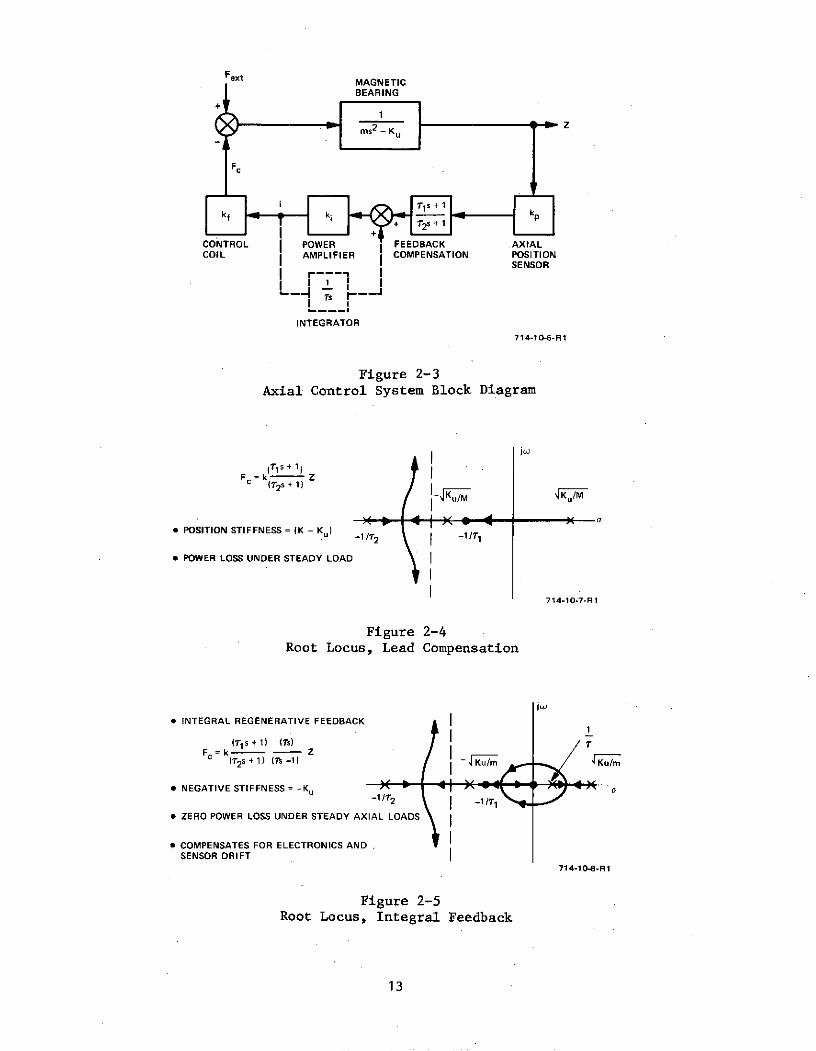
loss under external axial loads. In practice, the rate sensor may be avoided by

using lead compensation of the position signal. A block diagram of the axial

control system is shown in Figure 2-3, and the root locus in Figure 2-4.

In addition to the lead compensation, a minor loop integrator can be added

(shown by dashed lines in Figure 2-3), in order that the unbalance stiffness of

the passive magnetics can be used to advantage in overcoming external loads. The

integrator also enables long-term, low-power operation by correcting for drift in

any of the electronic components, including the position sensor. With integral

feedback, the static axial stiffness is negative; the root locus of this system

is shown in Figure 2-5.

12

BEARING

CONTROL POWER FEEDBACK AXIALCOIL I AMPLIFIER COMPENSATION POSITION

SENSOR

INTEGRATOR

714-10-6-R1

Figure 2-3Axial Control System Block Diagram

1w(

s + 1)

F =k Z( 2s+1)

* POSITION STIFFNESS = (K - Ku ) -1/1

* POWER LOSS UNDER STEADY LOAD I

714-10-7-Ri

Figure 2-4Root Locus, Lead Compensation

j w

* INTEGRAL REGENERATIVE FEEDBACK

" NEGATIVE STIFFNESS = -Ku A

" ZERO POWER LOSS UNDER STEADY AXIAL LOADS

" COMPENSATES FOR ELECTRONICS ANDSENSOR DRIFT

714-10-8.R1

Figure 2-5Root Locus, Integral Feedback

13

SECTION 3.0

REACTION WHEEL DESIGN

14

SECTION 3.0

REACTION WHEEL DESIGN

This section presents a discussion of the design tradeoffs leading to a pre-

ferred configuration for a magnetically suspended RWA. The design objectives are

interpreted in terms of RWA requirements, and specific component analyses are

developed. Conceptual RWA design approaches are compared and evaluated. A pre-

liminary RWA layout is presented for the preferred approach, along with calculated

design and performance parameters.

3.1 RWA DESIGN OBJECTIVES

The design specifications for the RWA are listed in Table 3-1. Those which

have the most influence on the design tradeoffs are listed separately as primary

specifications.

TABLE 3-1

RWA SPECIFICATIONS

PRIMARY DESIGN OBJECTIVES

Angular Momentum +.5 to -.5 ft-lb-sec

Motor Torque (minimum) -.01 to +.01 vt-lb

Motor Power (maximum) 8 watts

Bearing System Power (maximum) 8 watts (peak)

1 watt (average)

Cross Axis Rate (maximum) .0175 radian/second

Weight (maximum) 8 pounds

Volume (maximum) 250 inch 3

Temperature Range +200C to +750 C

Pressure (ambient) 10- 14 torr

Life (minimum) 10 years, operating

Shock and Vibration TBD

15

TABLE 3-1 (cont)

RWA SPECIFICATIONS

SECONDARY DESIGN OBJECTIVES

Radial Magnetic Field (maximum 10 nanotesla (10-4 gauss) at 1 meter

Radial Magnetic Field Variation 4 nanotesla at 1 meter, 0 to 30 Hz

Radiation Resistance 104 rads (silicon)

Bearing System Stiffness (nominal)

Radial (total) 330 lb/inAxial 2000 Ib/in

Bearing System Capacity (nominal)

Radial (total) 7 poundsAxial 25 pounds

The motor torque is the net (accelerating/decelerating) torque applied to the

wheel, and its reaction is useable for vehicle control purposes. This torque must

be delivered upon command in either direction over the total angular momentum range

of the wheel. The maximum motor power of 8 watts includes that required for bear-

ing and windage drag, in addition to the net torque delivered to the vehicle.

The cross axis rate input causes a deflection at each bearing due to gyro-

scopic effects (P x H). The interpretation of this requirement is that there be

no physical contact of the touchdown bearing elements during this condition.

The weight and volume requirements include the RWA plus one channel of bear-

ing control electronics. Spin motor control electronics and/or redundant bearing

control electronics are items for separate consideration.

Meeting the performance requirements at low ambient pressure and over the

stated temperature range should not be a problem as it is with ball bearing wheels.

Because magnetic bearings are low power devices and are directly compatible with

hard vacuum, the housing can be vented directly to space with no adverse effects

on the RWA. Performance over the temperature range should also be readily achieved

because of the absence of lubricants, and in fact, can be expected to show no

substantial variation from standard test conditions.

16

The 10 year life requirement does not apply in the normal mechanical sense

because wearout mechanisms are not present. Thus, the definition of life is re-

duced to determining the reliability of the magnetic bearing control system based

on constant failure rates. Redundancy, along with improved reliability, can be

achieved by duplication of the electronics to operate on a standby basis.

The external radial fields are difficult to assess analytically, and also

require a very sophisticated setup for measurement. (The earth's magnetic field

is approximately 50,000 nanoteslas.) The implication of this requirement in the

RWA design is to contain the fields and use opposing polarities in the magnetic

bearings, and to use non-magnetic materials whenever possible elsewhere.

The bearing system stiffness and capacities listed are actually those of

Sperry model bearing (Appendix A), and do not necessarily have a direct relation-

ship to the RWA design. The radial stiffness and capacity requirements are estab-

lished by the angular stiffness required to sustain x H torque loading by rotor-

bearing dynamics considerations and/or 1-g operation. Axial stiffness and capacity

are somewhat arbitrary within broad limits, and can be set to a desired value by

adjusting the servo gain.

3.2 COMPONENT ANALYSES

3.2.1 Inertia Element

For purposes of RWA optimization, which is defined as minimum weight, it

is necessary to characterize the total weight of the rotating elements in terms

of the radius of the rotor rim and rotor speed, considering the rotor to consist

of a rim attached by a web to a shaft on bearings. To develop the required re-

lationship, start by defining the ratios

Irim

I = (3-1)IR

WrimW rim (3-2)

WR

where

Irim = inertia of rotor rim

IR = total inertia of rotating elements

17

W . = weight of rotor rimrim

WR = total weight of rotating elements

Also, the inertia of the rim, considered as a thin hoop, is

I rim R2 (3-3)R g

where

R = rotor radius

The angular momentum (H) is given by

H60 N (3-4)

where

N = rotor speed (rpm)

Substituting Equations (3-1), (3-2) and (3-3) into (3-4) and rearranging yields

60 g H (I) (3-5)W 2-

2 = NR2 ()

The ratio (1)/(W) varies with the size and construction of the rotor. In

the size range of interest, a representative value can be taken as .6. For the

nominal angular momentum H = .5 ft-lb-sec,

W 36860 (3-6)R = 2

NR

where the units are pounds (WR), rpm (N) and inches (R). A plot of Equation

(3-6) is presented in Figure 3-1, with R treated as a parameter.

In determining the range of rotor radii and rpm, the following constraints

must be considered:

o Power-Limited Speed

For the case where maximum motor power and required RWA torque are

specified, the rpm is constrained by

N < 1352 !P (3-7)max T

18

26.25

R = 1"

22.5

18.75

R =2"

POWER LIMITED SPEED

(8 WATS, 2 OZ-IN)H = 0.5 FT-LB-SEC

11.25

R=3"7.5

R= 4" __

3.75

R = 5"

00 1000 2000 3000 4000 5000

N (RPM) . 714-21-1

Figure 3-1Total Rotor Weight (WR) versus Speed (N), H = .5 foot-pound-second

where

n = motor efficiency at Nmax

P = maximum motor power (watts)

T = motor output torque at N (oz-in)max

The specified torque is .01 ft-lb = 1.92 oz-in. With allowance for

the additional torque due to magnetic bearing drag, T = 2 oz-in can

be used for P = 8 watts; therfore

N < 5408 9 (3-8)max

Thus the theoretical maximum rpm that can be considered for the de-

sign, corresponding to 9 = 1, is 5408 rpm. The practical limit, using

an efficiency for an ac induction motor of n = .6, is 3245 rpm. This

constraint is shown in the curves of Figure 3-1.

* Minimum Rotor Weight

The minimum rotor weight must at least equal the sum of the motor cage,

shaft and magnetic bearing rotors. In this case W = 0, I = 0 and

Equation 3-6 does not apply. This constraint is dependent upon the

design approach taken for the rotor, and is examined in each indi-

vidual case.

* Rim Size

The rim weight and cross-section decreases rapidly with increasing

speed and increasing radius. Thus, once an optimal design is de-

termined, it is necessary to provide sufficient cross-sectional

area in the rim for the required rotor weight. This can be

accomplished by material selection and/or variation of the aspect

ratio of the trim cross-sectional area.

3.2.2 Spin Motor

The selection of a spin motor for a low angular momentum reaction wheel is

very dependent on the overall design concept of the unit. For this study the

effort was limited to ac induction type spin motors, based on the fact that they

have the highest efficiency of ac devices, and the failure rate of the motor con-

trol system is approximately one-half that of a brushless dc system.

20

The initial requirements used were the maximum power limit of 8 watts, a

minimum torque of 2 ounce-inches, and a minimum motor I.D. of 1.0 inch. The

parameter used to evaluate the motor design was weight. The initial motor design

was not constrained by the overall RWA design so as to provide the opportunity

for attaining any advantages of operating speed, form factor, excitation frequency,

number of poles, etc. A flow diagram of the motor optimization process is shown

on Figure 3-2.

Because of the power limitation of 8 watts, there is a maximum theoretical

operating speed limit. This speed is defined by Equation (3-7), which results in

a maximum speed (NR max) of 5408 rpm. In order to evaluate different motor de-

signs, it is useful to consider a measure of an induction motor performance

called "stall torque efficiency", es, which usually varies over a range of .2 to

.8. Stall torque efficiency is defined as

Pe _ -

s Pin

where

Ps = synchronous load power

P. = P + stator lossesin s

e is a function of motor weight, impedance and synchronous speed. Choosing a

value of es = .6, results in a maximum synchronous speed of

N = .6 (5408)max

= 3245 rpm

Note that this is coincidentally the same speed as derived in the paragraph 3.2.1

where the true motor efficiency (7) was used.

In order to provide the required torque over the operating speed range,

consideration of the torque-speed characteristic is necessary. Figure 3-3 shows

three possible torque speed characteristics which meet the requirement of minimum

torque over the operating speed range.

21

F----1PRELIMINARY INITIAL

REQUIREMENT WEIGHT VS N RWA RADIUS,CURVE OPTIMIZATION

MAXIMUM POWER (FIGURE 3-4) (PARA 3.3)

MINIMUM TORQUE _MINIMUM I.D.+N RPM

SELECTED MOTOR

MOTOR 3.5-IN. RADIUS OPTIMIZE 3.5-IN. RADIUSRADIUS MOTOR, NUMBER 32 POLE

TRADEOFF 1500 RPM POLES 640 HzTWO-40 DEGSEGMENTS

714-21-31

Figure 3-2Spin Motor Optimization Flow

22

I-I

2.0

NMAX NS

N (RPM)714-21-2

Figure 3-3Induction Motor Torque/Speed Characteristics

The tradeoff studies showed that characteristic 2 was minimum power at con-

stant weight, and hence was selected as an intermediate design requirement. This

aspect of motor design is a function of the ratio .of rotor resistance to stator

reactance, and can be altered by changing the resistance (material composition)

of the conductors in the squirrel cage.

Prior motor design experience has shown that torque-speed linearity is

best achieved if the maximum operating speed (N ) is chosen between .5 N andmax s.7 N . In order to reduce the number of parameters involved in the tradeoff,s.6 Ns was chosen as the maximum operating speed. This reduced the RWA operating

speed range to N < 1950 rpm for best motor design.max

The following motor designs were developed at this point, and illustrate

the trend that can be expected.

ID Gap Dia Speed WeightMotor (in.) (in.) (rpm) (lb)

A 1.0 3.04 1250 .71

B 1.5 3.33 2000 1.75

C 2.125 3.63 2500 2.80

The data is plotted in Figure 3-4, and is used in the RWA optimization (Section

3.3) wherein rotor radius and speed are determined for the minimum weight system.

23

z

I

I

I

0.1

o 2 l

"I01

0 500 1000 1500 2000 2500 3000 3500

MAX OPERATING SPEED (RPM) 714-21-3

Figure 3-4Motor Design Optimization Curve

24

The RWA optimization process in Paragraph 3.3 demonstrated that signifi-

cant weight savings can be effected by utilization of a large diameter segmented

spin motor where the motor cage is also used as the primary inertia element.

This fact was incorporated in the motor design calculations, and a speed of

1500 rpm and a radius of 3.5 inches was selected for further optimization. This

resulted in the following physical characteristics for the spin motor:

Gap Diameter 7.0 in.

Weight

Cage 1.0 lb

Stator (2-40* segments) .6 lb

Poles 32

Excitation 25V, 640 Hz, 2 phase

Maximum Operating Speed (N ) 1500 rpmmax

The performance data (power and torque versus speed) is plotted in Figure 3-5.

Note that the minimum output torque is 2.2 ounce-inches and the nominal power

is 7 watts; these margins are sufficient to ensure that the requirements of

2 ounce-inches and 8 watts are met in actual production design.

25

18 - 2.6

16 - 2.4

14 - 2.2

12 - 2.0

TORQUE

10 - 1.8

8 - 1.6

7 - N 71.4

ww 6

_6 1.20 0 POWER

3 .6 I

32 POLE - 2-400 SEGMENTS25 VOLT, 640 Hz, 2 PHASESINE WAVE EXCITATION

1 .2 - NMAX = 1500 RPM

0- 0_0 2 4 6 8 10 12 14 16 18 20 22

SPEED (RPM X 10-2 )

NMAX 714-21-4

Figure 3-5Performance Data, Segmented Spin Motor

26

3.2.3 Magnetic Bearings

The rationale for selection of a dc magnetic, passive-radial, active-

axial bearing system was outlined in Paragraph 2.2. Following this, the influ-

ences of the actual bearing design on the overall RWA must be examined. The

achievement of angular stability dictates the use of two radial-passive bearings

with a sufficient axial spacing between them. The stabilizing torque of the

bearing pair due to the radial restoring forces then far exceeds the destabiliz-

ing torque of each individual bearing due to the axial unbalance forces, thus

achieving passive angular stability of the total suspension system. Suitable

touchdown means must be designed in order that electronic component failures

are safely negotiated before a redundant control system is powered on. Another

influence is on the design of the motor, in which the radial clearance must be

larger than conventional systems using ball-bearings. In.the ac induction

motors being considered this increase in radial clearance does not cause a

large penalty in motor performance.

In the remainder of this section the constraints on the radial stiffness,

the choice of bearing configuration and the design of the bearing are examined.

3.2.3.1 Stiffness Constraints

The design of radial-passive magnetic bearings and their sizing are

dependent primarily on the required radial stiffness for the application. The

constraints on the radial stiffness based on design considerations/requirements

for the reaction wheel are considered separately below.

a. Radial Capacity in a 1-g Environment

It is assumed that touchdown must not occur during operation or

test in any attitude, in either a O-g or a 1-g environment. The most stringent

condition is when the wheel is operated with axis horizontal in a 1-g environment,

and additional radial deflection due to motor unbalance and under cross-axis

rates must be allowed for.

For a magnetic bearing geometry using axially opposed concentric

rings a suitable constraint is to limit the allowable deflection under the self-

weight to one land width of the concentric ring. Thus

27

K > (lb/in.) (3-9)r 2T

where

K = required radial stiffness per bearing

WR = total suspended rotor weight (lb)

T = width of a ring land (in.)

To ensure that the unbalance stiffness ratio is a minimum, the smallest possible

T must be chosen; the minimum value consistent with manufacturability is T - .014

inch. The minimum radial stiffness is thus a linear function of the rotor weight

and the variation is plotted in Figure 3-5.

150

1-g CONSTRAINT

(Kr

100

I I I

50

RADIAL RESONANCEFREQUENCY CONSTRAINT( K r2 )

0 1 2 3 4 5WR (LBS) 714-21-20

Figure 3-6Minimum Radial Stiffness due to Ig Capacity and

Radial Resonance Frequency

28

b. Radial Resonant Frequency

Considering the rotor as a rigid body, the radial resonant frequency

(fr) isr1 r2

fr = 2 g (Hz) (3-10)r 2# WR

If a minimum fr is specified, the constraint on stiffness simplifies to

2 2I f W

K > r R (lb/in.) (3-11)r2 6g

where

K = required radial stiffness per bearing2

WR = rotor weight (lb)

g = 32.2 ft/sec2

Since it is desired to maintain wheel resonances above 20 Hz to avoid interactions

with the spacecraft,

K > 20.45 WR (3-12)

which is a linear function, and is also plotted in Figure 3-5. It may be noted

that the Ig constraint on stiffness is more severe than that based on the radial

resonance frequency.

c. Angular Resonance Frequency

If the angular stiffness (K) is assumed to be due purely to the

radial restoring forces in each bearing, then

= 1/2 Kr 2 (in.-lb/radian) (3-13)

where

Kr = radial stiffness per bearing (Ib/in.)

2 = axial bearing span (in.)

29

In practice, however, the restoring torque due to the radial forces is diminished

by torques due to the axial unbalance forces. (The exact expression for the

angular stiffness is obtainable only as a derivative of the total co-energy of the

system w.r.t. the angular displacement.) On the basis of laboratory measurements,

a conservative value for preliminary design is

K = 1/4 Kr p2 (3-14)

The angular resonance frequency for the RWA is a function of wheel

speed because of the gyroscopic interactions; however, the minimum resonance fre-

quency (f ) corresponds to the nonrotating condition and is given by

1 Kaf - (Hz) (3-15)

t

where

K = the angular stiffness (in.-lb/rad)

2I = the transverse inertia of the rotor (in.-lb-sec2)t

Solving Equation (3-14) and using a specified minimum of f ,

K > 472 f 2 it (3-16)

The rotor polar inertia (IR ) is typically 60 percent of the transverse

inertia (It). Combining this relationship with Equation (3-6) and substituting

into Equation (3-15) yields the following constraint: (H = .5 ft-lb-sec).

Kr > 58.92 WR lb/in. (3-17)

where

K = required radial stiffness per bearingr 3

WR = rotor weight (lb)

R = rotor radius (in.)

2 = axial bearing span (in.)

30

This equation is plotted in Figure 3-7 as a function of the rotor

weight (WR) and the ratio R/k for expected values in the RWA.

Rq 1.2

/ 0- .0

0- 0.

0 1 2 3 4W

R (LBSI) 714 21-33

Figure 3-7Minimum Radial Stiffness due to Angular Resonance Frequency

d. Cross-axis Rate

Under a cross-axis rate q the angular deflection (a) is given by

12 S2Ha = (radians) (3-18)

where

S= the angular stiffnes (in -ib/radian)

H = the angular momentum (ft-lb-sec)

The angular deflection is related to the radial deflection (6) at each bearing

by

2 8a = (3-19)

where 2 is the axial bearing span. Substituting for K in terms of Kr gives

the constraint

K > 24 H (3-20)

31

For H = .5 ft-lb-sec, and the specified value of 12= 17.5 mr/sec,

Kr > 21 b/in.

where 2 and S are in inches.

Thus, if we consider £ = 3 inches and 6 = .001 inch as minimum values,

this constraint gives

K > 70 lb/in. (3-21)r4

The above four constraints [Equations (3-9), (3-12), (3-17), (3-20)]

considered determine a minimum value of radial stiffness of the magnetic bearing.

Examination shows that for R/2 > .6 the constraint due to angular resonance fre-

quency dominates those due to the 1-g radial capacity and the radial resonance

frequency. In addition, if R/2 > 1, the constraint also dominates that due to

maximum cross-axis rate for WR > 1.2 pounds. For the representative value R/2 =

1.0, the required radial stiffness ranges from 70 pound/inch for a rotor weight

of 1 pound, to 167 pound/inch for a rotor weight of 3 pounds. Selection of the

final value of Kr is made in paragraph 3.2.3.3.

It may be noted that no restriction has been placed on the location

of the resonance speeds relative to the range of operating speeds for the RWA.

Thus, it is possible that a radial or angular resonance speed may be traversed

during wheel operation. This decision was based on tests on the Sperry magnetic

bearing model where it was determined that resonance speeds could be dwelt on for

extended periods without significant increases in motor or bearing power; the

radial excursions were also well-bounded. If the resonance speeds were con-

strained to be above the operating range, this would entail an unduly large

bearing radial stiffness with an attendant penalty in bearing weight.

3.2.3.2 Bearing Configuration

For implementing the radial-passive, axial-active, attraction concept

selected, the three-loop bearing configuration was used as a starting point.

(This configuration has been used for the Sperry magnetic bearing model as well

as for the suspension of a large 700 ft-lb-sec momentum wheel assembly.) Following

this, the one-loop bearing was examined as an alternative for the small RWA appli-

cation. This bearing concept, also previously developed, has the advantage of

simplicity. Both configurations are described below.

32

a. Three-Loop Bearing

A schematic of the configuration is shown in Figure 3-8. It is

termed a three-loop bearing because three independent loop equations are required

to analyze the magnetic circuit.

The bias magnetic flux (Bo) is provided by the axially magnetized

ring magnets across four axial gaps, the direction of the bias flux being shown

by the arrows in the figure. The passive radial stiffness is provided through

the action (minimum reluctance) of opposed concentric rings at the air gaps, the

total stiffness being proportional to the number of rings. Radial damping is

provided with conducting material, e.g., copper wire, placed between the rings

at the air gaps.

In the axial direction, the bias fields cause instability. Axial

control forces are provided by modulating the gap bias fluxes; this is accom-

plished by varying the magnitude and direction of the current to the two control

coils in response to a position error signal. Thus, the coils are connected

such that the bias flux is increased in one pair of gaps by an amount A B while

it is decreased in the other pair of gaps; the result is an axial force propor-

tional to 8B A B, as shown in Figure 3-9.

The significant features of the three-loop configuration can be

summarized as follows:

* Both magnets and coils are stationary

* The coil currents must overcome only the air-gap reluctance

* The axial stiffness obtainable is proportional to the bias

field, which permits higher gains at lower power levels

* Radial damping is provided by copper rings

* Pole pieces are used to minimize flux variations at the gaps

b. One-Loop Bearing

The terminology "one loop" here again refers to the fact that both

the permanent magnet and control coil establish flux in the same magnetic cir-

cuit loop, and the determination of this single loop flux is sufficient for a

magnetic circuit analysis. The one-loop bearing is shown in Figure 3-10.

33

&STATORPOLE PIECE

CONTROL COILS (2)BB

B

U//ISTABLE

714-10-4

Figure 3-8Three-Loop Bearing, Half Section

BIASFLUX PATH

CONTROL (Bo)FLUX PATH(AB) -AB +AB -AB +AB

FORCE ON ROTORFOR AB'S SHOWN

KCII F,

* Fa- [2(B o + A B)2 - 2 (Bo - AB) 2 1] 8B o0 AB

714-10-5* BI-DIRECTIONAL FORCES BY REVERSAL OF CONTROL CURRENT

Figure 3-9Axial Control Force Generation

34

714-21-22

Figure 3-10One-Loop Bearing Configuration

35

The bias flux is again provided by the permanent magnet, and passive radial stiff-

ness is attained through the action (minimum reluctance) of opposed concentric

rings. Bidirectional axial control forces are provided by modulation of the gap

flux by controlling the current in the coil.

The primary disadvantage of the one-loop configuration compared to

the three-loop configuration is that the control current must counter the reluc-

tance of the permanent magnet in the one-loop design. This means that larger

control currents are necessary to produce the same axial force, entailing larger

power loss under dynamic loads. In addition, high-coercivity permanent magnet

materials such as rare-earth cobalts are essential to prevent the possibility

of demagnetization. Analysis shows that the reduction in the force-to-current

gain because of the extra magnet reluctance is only 50 percent for the case

where the circuit is designed for minimum magnet volume, and can be lower at the

cost of some additional penalty in magnet volume.

Since the passive radial stiffness is proportional to the square of

the flux density, it is desirable to provide as high a bias flux density as

possible, allowing for sufficient margin for modulation before saturation. Con-

sidering that the flux density at saturation for soft material such as electro-

magnet iron is in the range of 1.6 to 2.0 Wb/m2 , a bias density level of 1.4 Wb/m2

is a suitable value for design; this leaves an adequate margin for modulation to

develop axial control forces.

Sizing a three-loop bearing for this bias flux density shows that

for a mean radius of .6 inch at the rings, and for merely 1 ring/gap, the radial

stiffness per bearing is

225 lb/in. 4 Kr < 554 lb/in.

where the upper limit is based on an infinite-width geometry stiffness analysis

and the lower limit on a line-potential geometry. Comparison with the required

radial stiffness for expected rotor weights (70 lb/in, to 167 lb/in.) shows

that the minimum radial stiffness in a three-loop bearing exceeds the require-

ments. The weight of such a three-loop bearing pair, including magnets, coils,

and pole pieces is estimated at 1.6 pounds.

36

Following this, a one-loop bearing was sized, for B = 1.4 Wb/m ,g

and a radius to the outer rings of .6 inch. The stiffness K was bounded inr

the range

167 lb/in. < Kr < 410 lb/in.

The weight of this bearing pair is estimated at .6 pound. The weight comparison,

the design simplicity, the fewer number of machined parts and ease of manufacture

and assembly were the basis for the selection of the one-loop design for this

RWA application. For the initial weight trade-off, the weight of the shaft and

stator support hardware was added to the actual bearing weight, and for the

expected stiffness range this total weight of the magnetic bearing system (W MB) is:

WMB = .4 WR (lb) (3-22)

3.2.3.3. Design of the One-Loop Bearing

Following the selection of the one-loop bearing configuration for the

RWA, the next step is the design of the magnetic circuit. Designing the magnetic

circuit involves the design of the gap geometries and magnetic structures, choice

of magnetic materials, and sizing of the permanent magnet and the control coil.

An important design parameter to be established at this point is the unbalance

stiffness ratio. This is the ratio of the axial unbalance stiffness to radial

stiffness for the passive magnetics and is the main parameter coupling the radial

and axial axes.

a. Radial System

The preliminary analyses on RWA sizing indicate that the total rotor

weight is likely to be in the range of 2 to 3 pounds. The design value for radial

stiffness is therefore taken as 167 pounds/inch, corresponding to the 3 pound

rotor weight. For the one-loop bearing, the initial radial stiffness is given

by

K r = 0 a (nl r1 + n r2 ) Bg (3-23)

37

where

a = coefficient dependent on geometry

n1 = number of rings at radius rl

n2 = number of rings at radius r2

and

B = the peak flux density in the gap.

In order that the axial spacing between bearings is not excessive,

a value rl = .6 inch is taken as a constraint. For B = 1.4 Wb/m 2 , the remainingg

values for a ring width T = .014 inch work out to be n1 = 2, rI = .3 in., r2 = 2.

The magnet material chosen for the design is.samarium-cobalt, be-

cause of

9 Its high energy-product, allowing a decrease in weight

over Alnico

o Its reversible, straight-line demagnetization characteristic

and high intrinsic coercive force. This is especially

important in the one-loop bearing design, because the con-

trol flux, which passes through the magnet, will oppose the

permanent magnet flux when it is desired to decrease the flux

density in the gap. The B-H characteristic also enables

the magnet to be magnetized prior to assembly and eliminates

the need for keepers.

Sizing the magnet for a nominal axial gap of .015 inch and B = 1.4

Wb/m2 gives

A =1.3 in.2 , 2 = .120 in.m m

where A is the cross-sectional area of magnet and £ is the axial length. Them mmagnet is designed to operate at its (BH)max point, to give minimum volume of

magnet material.

38

b. Axial System

The objectives here are to determine the expected axial unbalance

stiffness, the net axial stiffness under feedback and the required coil ampere

turns.

For the chosen geometry, the unbalance stiffness ratio is estimated

as

KK - -8 (3-24)r

The total axial unbalance stiffness (for both bearings) that must

be overcome by the axial control system is

K = -2 x 8 x 167 = -2672 lb/in.u

Under position-rate feedback, with the requirement that lift-off and control be

possible from a single coil (i.e., allowing for the provision of redundancy),

the feedback position gain for stability is

K v= 35.9 AT/M = 91,000 AT/in.

Considering a maximum axial travel before touchdown of .008 inch,

the required coil capacity for lift-off is 8 x 91 = 728 AT. The achievement of

net axial stiffness means that some margin must be provided above this. A value

of 1100 AT is chosen. Having determined the basic parameters for the design, the

pole pieces (to be made from electromagnet iron) and the control coils are sized

suitably to complete the design. In order to prevent clamping and reaction

forces being applied to the magnets, a non-magnetic spacer is used to separate

the stator pole pieces.

3.2.4 Suspension Control System

The suspension electronics provides the axial control forces to maintain

levitation of the rotor. The main components, as shown in Figure 3-11, are the

axial position sensor, compensation network, power amplifier, and an integrator.

Power consumption is minimized by the integrator, which causes the system to

operate at zero steady-state coil current. The primary design considerations

are maximum reliability and minimum power consumption.

39

SENSOR NETWORK AMPLIFIER

+- COIL

INTEGRATOR

CURRENTSENSERESISTOR

714-21-15

Figure 3-11Suspension Electronics Block Diagram

40

3.2.4.1 Position Sensors

Various types of noncontacting position sensor are capable of measuring

distances on the order of .005 to .035 inch, as required in this application.

Of these, the two offering the most advantages are the capacitive transducer

and the eddy current transducer.

The capacitive transducer, Figures 3-12 and-3-13, contains an ac source

and two capacitors which are the two parts of a differential capacitor. The

capacitor plates are discs. The center plate is fastened to the rotor shaft, and

the two outside discs are mounted on the frame but are electrically insulated

from it. For an axial displacement to the left in Figure 3-12, capacitor Cl will

increase and C2 will decrease in capacitance. This change is detected by the

sensor electronics and results in an error signal output to the suspension

electronics.

Since the rotor is suspended magnetically, there can be no physical

electrical connection to the shaft. The electrical circuit is completed by

means of capacitor Cs between the shaft and ground. This consists of the capa-

citance between the rotor and the fixed elements of the wheel, i.e., the housing,

the center tie bar, etc. This capacitor must be large compared to the elements

of the differential capacitor.

The capacitive transducer is simple, has good linearity and is insensi-

tive to temperature variations and variations of the source frequency. For a

plate area of .5 square inch, a sensitivity of .140 volt per mil of displacement

is achievable.

In the eddy current sensor (Figures 3-14 and 3-15) an ac source excites

a probe which is simply a small coil of wire oriented so that the induced field

intersects the sensed surface.* The surface must be a conductor so that eddy

currents are induced into it. The closer the probe to the sensed surface, the

greater the eddy currents will be.

The electronic circuit converts the eddy current variations into a dc

signal. The ac oscillator excites the probe through a high source impedance.

The voltage across the probe then varies as the coil impedance changes. The

voltage is converted to dc by rectification and filtering.

41

Cl C2

ROTOR SHAFT

I

T CS

TO ELECTRONICS 714-21-18

Figure 3-12Differential Capacitor

OSCILLATOR

R0 OUTPUT

R

C1 C2

CS

T 714-21-19

Figure 3-13Capacitive Transducer Circuit

42

ROTOR SHAFT

PROBE

ELECTRONICS

714-21.16

Figure 3-14Eddy Current Sensor

+

OSCILLATOR

S0 OUTPUT

PROBE

I 714-21-17

Figure 3-15Eddy Current Transducer Circuit

43

The eddy current sensor can provide an output scale factor of .3 volt

per mil and has good linearity. It is somewhat sensitive to temperature and

excitation frequency changes, but in the magnetic bearing application this is

not critical.

In choosing between the capacitive transducer and the eddy current

sensor, the main consideration is mechanical, i.e., the mounting of the probe

versus the plates or rings in the wheel assembly. The probe of the eddy current

sensor should be mounted directly at the center of the end of the shaft to

minimize pickup of angular motions and mechanical runout. Otherwise signals at

the rotational frequency will be input to the suspension electronics, resulting

in additional steady state power. The capacitive sensor with rings around the

shaft will average out any rotational frequency inputs.

The eddy current sensor was chosen for the RWA because of the less com-

plicated mechanical interface - while the capacitive sensor has some advantages,

they were not sufficient to warrant its use in a small wheel of this nature.

3.2.4.2 Power Amplifier

The power amplifier consists of a bridge which controls currents in

either direction through the coils in response to signals from the position sen-

sor. The compensation in the form of a lead/lag network, is included as a part

of the amplifier. Figure 3-16 is a schematic of the amplifier showing the use

of several operational amplifiers. The availability of new microcircuits con-

taining four, very low-power operational amplifiers on a single chip makes it

advantageous to replace discrete circuits with these devices. One small penalty

associated with the use of operational amplifiers is that it is necessary to

generate plus and minus power voltages from the +28 volt dc input power. The

use of ±8 volts used with 5 volt signals is selected over the more common ±15

volts and 10 volt signals to conserve power. Each operational amplifier will

use less than 5 milliwatts of power. The net savings of number of components

and power consumption justifies this approach.

The maximum permissible power consumption of the suspension system is

1 watt. This is achieved with considerable margin as seen in the next paragraph.

The maximum power consumption at lift-off is 8 watts. This is accomplished by

designing the coils to have a relatively high resistance by using many turns of

small wire which limits the amount of power that can be drawn from the +28 volt

44

-8 +28 VDC

LEAD LAG

POSITIONSENSOR

+8

-8 COILS

+8

INTEGRATOR

-8

-8

+28 ±8 VOLT +8

VDC POWERSUPPLY -8

714-21-14

Figure 3-16Power Amplifier Schematic

line when the amplifier is turned on. The force capacity of the coils is reduced

this way, but it is possible to maintain adequate capacity and still reduce the

total power to under 8 watts.

3.2.4.3 Power Breakdown

The calculated power consumption of the suspension electronics is given

in Table 3-2. This assumes that the wheel speed is not at any of the resonances

and that the position sensor is situated so that very little rotational motion is

detected. The position sensor contains an oscillator operating at 1 megahertz.

In the power amplifier, the bridge uses some power because it is impossible to

eliminate all rotary motion effects and other disturbances from the input. The

power supply provides ±8 volts for the position sensor and the operational ampli-

fiers, and it operates with an efficiency of about 50 percent.

TABLE 3-2

CONTROL ELECTRONICS POWER CONSUMPTION

PowerComponent Power

(mw)

Position Sensor 96Power Amplifier

Operational Amplifiers 20Bridge 140

Power Supply 116

Total 372

3.2.4.4 Reliability

The failure rate of the suspension electronics is estimated to be less

than one failure per million hours. The breakdown is as shown in Table 3-3.

TABLE 3-3

ELECTRONICS RELIABILITY

Component Quantity Total Failures per 106 hr

Sensor 1 .050Power Bridge 26 .196Op Amps 4 .510Power Supply 10 .104

41 .860

46

3.2.5 RWA Housing

The housing for the magnetic suspension reaction wheel assembly is basi-

cally a cylinder whose radius varies with rotor radius and whose height is rela-

tively constant. The height is determined primarily by the magnetic suspension

system which requires a length/diameter ratio = 3.0 with a minimum diameter of

1.0 inch. The mounting of the axial proximeter adds .6 inch to the overall

height, resulting in a basic configuration as shown in Figure 3-17. The weight

of the housing is the sum of the weights of the five basic parts as shown. All

material in the housing is aluminum.

4.44.0

Figure 3-17RWA Housing Weight Model

The weight of the housing is shown in the table below for 1 < R < 5

(R = Rotor radius) in terms of each element, and is plotted on Figure 3-18.

Rotor Element

Radius 1 2 3 4 5 Total (lb)

1 .188 .264 .108 .093 .025 .678

2 .565 .264 .203 .161 .072 1.265

3 1.01 .264 .288 .299 .148 1.939

4 1.57 .264 .374 .297 .247 2.752

5 2.26 .264 .460 .364 .372 3.720

47

4

3'

C2

00 1 2 3 4 5 6

ROTOR RADIUS R (IN) 714-21-7

Figure 3-18Housing Weight Versus Rotor Radius

48

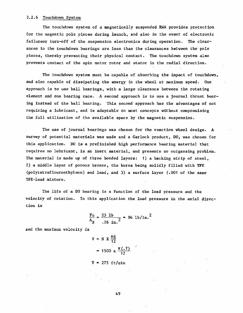
3.2.6 Touchdown System

The touchdown system of a magnetically suspended RWA provides protection

for the magnetic pole pieces during launch, and also in the event of electronic

failureor turn-off of the suspension electronics during operation. The clear-

ances in the touchdown bearings are less than the clearances between the pole

pieces, thereby preventing their physical contact. The touchdown system also

prevents contact of the spin motor rotor and stator in the radial direction.

The touchdown system must be capable of absorbing the impact of touchdown,

and also capable of dissipating the energy in the wheel at maximum speed. One

approach is to use ball bearings, with a large clearance between the rotating

element and one bearing race. A second approach is to use a journal thrust bear-

ing instead of the ball bearing. This second approach has the advantages of not

requiring a lubricant, and is adaptable to most concepts without compromising

the full utilization of the available space by the magnetic suspension.

The use of journal bearings was chosen for the reaction wheel design. A

survey of potential materials was made and a Garlock product, DU, was chosen for

this application. DU is a prefinished high performance bearing material that

requires no lubricant, is an inert material, and presents no outgassing problem.

The material is made up of three bonded layers: 1) a backing strip of steel,

2) a middle layer of porous bronze, the bores being solidly filled with TFE

(polytetraflouroethylene) and lead, and 3) a surface layer (.001 of the same

TFE-lead mixture.

The life of a DU bearing is a function of the load pressure and the

velocity of rotation. In this application the load pressure in the axial direc-

tion is

Fu 25 lb 96 b/in. 2- = 96 lb/in.B .26 in,2

and the maximum velocity is

ndV= NX

12

r(.7)= 1500 x12

V = 275 ft/min

49

The product PV = (275)(96)

= 26400

The life (H) at this load rating for a thrust bearing, which is the load situa-

tion for a touchdown is

12 x 106PV--

H + 200

12 x 106H -200

PV

12 x 106= -20026400

= 455 - 200

H = 255 hrs

Since this application is one that is encountered only in test and for a failure

mode during operation, the life is adequate.

The coefficient of friction for these conditions (< 500 psi, 10 < V <

1000 fpm) is 0.1-0.2, which produces a torque of

T = .2 (25) (.35)

= 1.75 in. lb

T = 28 oz in.

The energy in the reaction wheel at maximum speed (1500 rpm) is

E = 1/2 HW

27= 1/2 (.5)(1500)(-~)

E = 39.3 ft lb

= .0506 BTU

The bearing material has a specific heat of .2 BTU/lb OF, and weighs

.004 pound. The temperature rise during a touchdown from 1500 rpm is 630F which

is well within the operating limit of the material.

50

The load rating of DU for fluctuating loads at less than 105 cycles is

4000 psi, which provides adequate margin for the conditions encountered in a

touchdown situation.

The shock and vibration capability of a ball bearing reaction wheel is

usually limited by the load carrying capacity of the bearings. The ball bearings

are stiff, resulting in relatively high natural frequencies, which are associated

with the higher energy inputs. The bearings must not be brinelled by these loads

in order to rpvode smooth operation on orbit.

The magnetically suspended reaction wheel, however, is designed such that

these launch loads are taken by the touchdown system, which is not in contact

during operation, and hence must only survive without deformations of more than

.003-.005 inch. The contact surface in a journal type touchdown system is signi-

ficantly larger than that of a ball bearing, which is another factor in the shock

and vibration capability of the design. The effect of the nonlinear nature of the

clearance in the touchdown system has not been evaluated, but should also be a plus

feature because of its inherent damping.

It is expected that the magnetically suspended reaction wheel will not

encounter any significant problems due to shock or vibration loads.

51

3.3 RWA DESIGN CONCEPTS

The three primary elements in a reaction wheel optimization are:

* Rotor

* Housing

* Spin Motor

The peak power requirement of this study places an upper limit on maximum operating

speed, but does not limit the optimization process, as will be seen later. The

three primary components used in the tradeoff can take many different character-

istics depending on the general configuration desired. For example, the spin

motor length/diameter ratio can vary from a typical servo motor shape to a pan-

cake configuration. The housing can vary from a cg mount to an end mount, and

can be round or square. The rotor web can be spoked, flat, conical, or umbrella

and when combined with a large diameter motor cage, could require little or no

rim. The large OD pancake type motor lends itself very nicely to the concept

of a redundant motor stator, since the torque capability increases rapidly with

diameter, usually requiring only a portion of the 360 degrees available for the

stator.

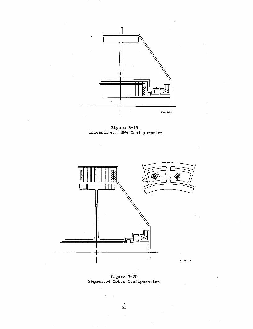
Two possible concepts are shown on Figures 3-19 and 3-20 as examples of the

extremes that the RWA configuration can take. The general shape of the magnetic

suspension elements can also affect the optimization process.. If these elements

are mounted in a manner similar to that shown in Figures 3-19 and 3-20, the re-

sult is a longer axial dimension, and hence increased housing weight. The most

weight effective design approach results in a dense package with the inertia ele-

ment at as large a radius as possible. This philosophy resulted in the concept

shown in Figure 3-21. The fact that the touchdown system is embodied in the

covers and the irregular mounting base configuration were not among the most de-

airable features. These were corrected in the concept of Figure 3-22. It was

this basic configuration that was used in the optimization process.

The basic component weight curves are shown in Figures 3-1, 3-4 and 3-18.

Combining this data, and approximating the magnetic suspension weight as .4 times

the rotor weight [Equation (3-22)] results in the RWA weight curves shown in

alternate forms in Figures 3-23 and 3-24. This optimization indicates that a

wheel of 3 to 4 inches radius at 1000 to 2000 rpm should be minimum weight.

52

+714-21-24

Figure 3-19Conventional RWA Configuration

600

714-21-23

Figure 3-20Segmented Motor Configuration

53

3.1

5.0 DIA - 714-21-13

Figure 3-21

RWA Design Concept, Configuration A

54

714-21-12

Figure 3-22RWA Design Concept, Configuration B

55

17.5

N =1000 RPM

15.0

12.5

2300 RPM

1 - 2 0 0 0 R P M-,

. 7.5

5.0

2.5

N = WHEELSPEED (RPM)

01 2 3 4 5

ROTOR RADIUS (INCHES) 714-21-25

Figure 3-23RWA Weight Versus Rotor Radius

56

17.5

R=2

15.0

12.5

0 10.0

R = 3 INCHES-I-

S7.5

R=4

5.0

2.5

R =

ROTOR RADIUS (INCHES)

00 1000 2000 3000 4000

ROTOR SPEED (RPM) 714-21-26

Figure 3-24RWA Weight Versus Rotor Speed

57

Realizing that rotor weight and inertia vary with radius, and that motor

configuration constraints do affect weight, a further tradeoff was made to deter-

mine the preferred motor. At the selected speed of 1500 rpm and 3.5 inch radius,

one configuration utilizing a 360 degree, 2.0 inch radius motor was compared with

a configuration using a segmented motor at 3.5 inch radius. The two configura-

tions are shown schematically in Figures 3-25 and 3-26.

The weight comparison is as follows:

2-inch motor radius 3.5-inch motor radius

Rotor 2.07 1.70

Stator 2.00 .60

Housing 2.52 2.84

Magnetic Suspension .90 .90

7.49 lb 6.04 lb

In addition to providing a weight advantage, the larger segmented motor provides

the opportunity for a redundant spin motor, in addition to providing space for

redundant bearing electronics and drive electronics if desired.

Based on a comparative evaluation of these design concepts, the segmented

motor approach was selected wherein the motor cage serves as the prime inertial

element. A preliminary layout of this concept is discussed in the following

section.

3.4 PRELIMINARY DESIGN LAYOUT

The preliminary layout of the selected configuration is shown in Figure

3-27, which includes the segmented spin motor and the single loop magnetic sus-

pension. The unit, as shown, is 8.9 inches in diameter and 4.6 inches high, and

weighs 6.52 pounds.

The magnetic suspension configuration lends itself to the concept of machin-

ing after final assembly to establish the magnetic gaps and the touchdown system

clearance. This approach is possible due to the mounting of the suspension system

in a tube. The magnetic suspension elements are cylindrical in shape, stack in-

side the tube, and are secured by the nut at the upper end of the tube. The ele-

ments can be assembled in a fixture, which is a tube mounted on a base plate.

58

MAGNETIC BEARINGASSEMBLY

nD. (SEE FIG 3-22)

MOUNTINGBASE /

"ELECTRONICS

7/ /-/// 777714-21-27

Figure 3-25RWA Design Concept, Configuration C

COVER

SEGMENTEDMOTORSTATOR

MOTORCAGE

MAGNETIC BEARINGASSEMBLY

a% (SEE FIG 3-22)

MOUNTINGBASE

ELECTRONICS

714-21-28

Figure 3-26RWA Design Concept, Configuration D

TOUCHDOWNBEARING

MAGNETIC BEARINGROTOR POLE-PIECE

MAGNETIC BEARING CONTROL COIL PERMANENT MAGNETSTATOR POLE-PIECES CLAMPIGNUT

ROTOR

ETSPACER RING

COVER

MOTOR SUPPORT

MAGNETBRACE ~ MOTOR BACKINGPLATE

SEGMENTEDROTOR SHAFT - MOTORSTATOR

(400)

r tMOUNTINGBASE

VENT CONNECTOR

VALVE

ELECTRONICS

POSITIONEND CAP SENSOR TACHOMETER 714-21.29

Figure 3-27Preliminary RWA Design Layout

The tube is machined with access ports in the area of the lower magnetic gap,

permitting measurement of the gap. A slot will be machined in the assembly tube

in the axial direction to permit the angular alignment of the magnetic suspension

elements during final assembly to minimize runout effects.

The layout is shown with a flush end mount to simplify the mechanical inter-

face. A center of gravity mount would result in some weight savings, better

utilization of the available volume, and potentially reduced vibration

susceptibility.

The configuration also permits running of the unit without the cover which

simplifies the instrumentation for calibration and test. The segmented spin

motor provides the opportunity for adding a redundant motor stator without com-

plicated redesign or any weight penalty other than the additional stator. The

configuration also provides room for integral packaging of the suspension elec-

tronics, either single channel or redundant, and the spin motor drive electronics,

if desired.

The preliminary layout (Figure 3-27) was used as the model for assessing the

weight of the entire unit. The weight summary is listed in Table 3-5.

TABLE 3-5

MBRWA WEIGHT SUMMARY

WeightComponent (ib)

Housing

Base 2.36Cover .55

Rotor

Web .90Cage 1.00

Magnetic Suspension .92

Motor Stator .60

Electronics .15

Connectors .06

Vent Valve .04

Electronics Mount .02

Proximitor .02

TOTAL 6.62

62

The materials used for assessing the weight of the unit were as follows:

Case/Cover Aluminum alloyShaft Titanium alloyWeb Titanium alloySuspension spacers Titanium alloyPole Pieces Magnet iron

The detailed design process for the unit would consider the use of beryllium for the

case/cover, shaft, and suspension spacers. In addition to effecting a weight reduc-

tion of approximately 1.3 pounds, the temperature sensitivity would also be reduced.

The tachometer shown in the layout is a simple variable reluctance pickup

which was intended for use as a speed indicator for wheel unloading purposes. The

vent valve is used to open the unit to the vacuum of space on orbit to prevent any

buildup of pressure within the unit. This is desirable to maintain the predicted

power levels over the 10 year life of the unit. Unlike ball bearing units, the

magnetically suspended unit is not subject to lubricant loss problems, and thus

can take full advantage of venting.

One feature of the design is the full containment of the permanent magnets,

and the spacer ring between the pole pieces. These items eliminate the two major

limitations of permanenft magnets of this type, which are the presence of micro-

cracks which could lead to particle generation and relatively low strength. The

full containment feature of the design contains any particles, and the pole piece

spacer removes mechanical load from the magnets.

It also should be noted that the design could be made without a cover. This

is possible due to the restricted path available for admitting external contamina-

tion and no requirement for containing any lubricant. This feature would result

in a unit weight of approximately 4.4 pounds when combined with the beryllium

material substitution and a cg mount.

The preliminary design was based on a peak spin motor power of 8 watts and a

momentum of ±.5 ft-lb-sec. If it is desired to reduce the spin motor power to 4

watts, this can be accomplished by increasing the motor stator weight and running

the unit at the same speed or by increasing the rim weight and reducing the speed

to one half of its present value. The motor efficiency is .278 at full speed with

the present design, and it certainly could be increased to .56 by addition of more

iron. Reducing the maximum speed to 750 rpm and increasing the rim weight by 1.2

pounds also effects a 4-watt reduction in power. This results in a sensitivity of

no more than .3 pound per watt for a range of at least ±4 watts about the nominal

8-watt value.

63

SECTION 4.0

CONCLUSIONS

64

SECTION 4.0

CONCLUSIONS

This design study has resulted in the following conclusions concerning a

magnetically suspended reaction wheel:

* The MBRWA is competitive with current ball bearing reaction wheels

in terms of weight, power, and cost.

* The design completely eliminates all single point failure sources

in a single mechanical assembly.

* The suspension electronics represents the only limitation of

storage or operational life of the unit.

* The design eliminates the increase of spin motor power with low

temperature and life that is encountered in ball bearing units.

* The magnetically suspended reaction wheel is much more tolerant

to shock or vibration loading than a ball bearing unit because

of the physical separation of the load carrying surfaces and the

on orbit rotational suspension.

* The sensitivity of the design is

Spin motor peak power .3 lb/watt

Suspension peak power .025 lb/watt

Momentum 2.4 lb/ft-lb-sec

Redundant spin motor .6 lb/motor

* The design configuration provides the opportunity for integral

mounting of suspension and spin motor drive electronics, redun-

dant spin motor, and inherently provides redundant suspension

coils.

* The design weight can be reduced to 4.4 pounds by use of selected

materials and the elimination of the cover, which is not required

on orbit.

* The MBRWA design which resulted from the study meets the design

objectives set forth in the Statement of Work. The major design

objectives and the resulting performance are listed in Table 4-1.

65

TABLE 4-1

MAJOR DESIGN OBJECTIVES

Parameter Design Objectives Attained Value

Angular Momentum ±.5 ft-lb-sec ±.5 ft-lb-sec

Weight 8.0 lb 6.62 lb

Size 250 in. 220 in. 3 (8.9 in. diameter x4.6 in. high)

Cross Axis Rate 17.5 mr/sec 832 mr/sec

Output Torque .01 ft-lb .01 ft-lb

Motor Power (maximum) 8 watts 8 watts

Bearing Power

Maximum 8 watts 8 watts

Average 1 watt .5 watt

66

SECTION 5.0

RECOMMENDATIONS

67

SECTION 5.0

RECOMMENDATIONS

Based on the conclusions presented in Section 4.0, it is recommended that

a hardware development program be initiated for a magnetically suspended RWA.

This program would be composed of two phases, leading eventually to a qualified

flight model. The first program phase is an engineering development, based on

the presently recommended design approach, and would result in an engineering

model suitable for functional and environmental testing. At the completion

of this development effort, a flight unit would be designed and qualified

to a detailed equipment specification.

A program plan for RWA development (Phase I) is presented in the remainder

of this section, and consists of detail task descriptions and a program schedule

(Figure 5-1). The duration of this development program is 12 months, and it is

estimated that the follow-on flight qualification (Phase II) would require an

additional 18 months.

TASK DESCRIPTIONS

1.0 Preliminary Design Requirements

Outline of RWA design requirements, based on the specified performance,

interface and environmental requirements of the intended application.

2.0 Design Analyses

Based on the results of Task 1, detail design analyses will be prepared to

establish the critical component parameters. Preliminary estimates of RWA weight

and power will also be made.

3.0 Component Development Tests

These tests comprise those necessary to verify the design approach in cer-

tain areas; principal among these is the operability of the touchdown system.

68

MONTHS AROTASK

1 2 3 4 5 6 7 8 9 10 11 12 13 14 15 16 17 18 19 20

1.0 PRELIMINARY DESIGN REQUIREMENTS

2.0 DESIGN ANALYSES

3.0 COMPONENT DEVELOPMENT TESTS

4.0 DRAWING PREPARATION

5.0 PARTS PROCUREMENT

6.0 TEST EQUIPMENT/FIXTURES

7.0 ASSEMBLY AND CALIBRATION

8.0 FUNCTIONAL TEST

9.0 ENVIRONMENTAL TEST

10.0 FINAL REPORT

11.0 EQUIPMENT DELIVERY

714-21-30

Figure 5-1RWA Development Schedule, Phase I

69

4.0 Drawing Preparation

A layout will be made from which detail drawings can be prepared for parts

procurement and/or fabrication. Final weight calculations will be made from

these drawings.

5.0 Parts Procurement

Parts will be procured for the engineering model. The spin motor is expected

to be the only long lead item, and its development will be coordinated with a

vendor during the design analysis task.

6.0 Test Equipment and Fixtures

Special test equipment and holding fixtures will be designed and fabricated.

7.0 Assembly and Calibration

Assembly and calibration of the RWA, including component performance data

verification, wheel dynamic balance and bearing control system evaluation.

8.0 Functional Test

Testing of the RWA to evaluate operability and performance. Major parameters

of interest are power (transient and steady state), drag torques, cross axis

rates, rotor/bearing dynamics, touchdown system and spin motor performance.

9.0 Environmental Test

Measurement of performance under thermal vacuum exposure; sinusoidal vibra-

tion survey to determine primary resonances; random vibration exposure.

10. Final Report

Description of development results, with recommendations for flight hardware

design.

11.0 Equipment Delivery

Refurbishment (as required) and delivery for test at JPL.

70

SECTION 6.0

NEW TECHNOLOGY

71

SECTION 6.0

NEW TECHNOLOGY

The technical information contained in this report is based on prior develop-

ments at Sperry Flight Systems, in the areas of reaction wheel assemblies, motors

and magnetic bearings. There was no new technology developed during the course

of this contract.

72

APPENDIX A

DESCRIPTION OF THE SPERRY MAGNETIC BEARING MODEL

73

APPENDIX A

DESCRIPTION OF THE SPERRY MAGNETIC BEARING MODEL

The Sperry magnetic bearing model, which uses a unique three-loop design, is

described in this appendix. The purpose is to provide background data, developed

prior to this present JPL study effort, which substantiates certain decisions

made during the course of the RWA design as described in Section 3.0 of this

report. The results are especially applicable because the bearing radial stiff-

ness is nearly the same as required in the .5 ft-lb-sec RWA. A photograph of this

model is shown in Figure A-i.

A.1 PHYSICAL DESCRIPTION

The magnetic bearing model was constructed in order to verify design

approaches and to obtain test data prior to application of magnetic bearings to

a large (700 ft-lb-sec) reaction wheel assembly. The cross-section of each

individual bearing is shown in Figure A-2.

The model consists of a shaft mounted on two magnetic bearings, with pre-

loaded ball-bearings at each shaft end provided for touchdown during shaft rota-

tions. An ac induction motor is used for application of torque about the spin

axis. Samarium-cobalt magnets establish a quiescent flux between axially opposed

soft iron rings, this flux being modulated by the control coils to provide axial

control forces. Radial damping is provided by copper wires which are cemented in

the pole-face grooves at the magnetic gaps. The axial control system utilizes a

single lead-lag network for compensation, with a current amplifier to drive the

coils. Provisions were made for test with or without the positive integral feed-

back technique (Paragraph 3.2.3). Eddy-current proximeters are used both for

axial position sensing, as well as for monitoring radial displacements.

A.2 TEST RESULTS

The test model has been successfully levitated and rotated at speeds up to

11,500 rpm, both in air and under evacuated conditions. Successful operation of

the ball bearing touchdown system has also been achieved over this speed range.

Very stable suspension has been attained, with minimal power loss under both

ambient conditions and steady external loads achieved with the use of positive

integral feedback of control current.

74

714-21-8

Figure A-1

Magnetic Bearing Model

75

RINGSUPPORT MAGNET

SOFT IRONFLANGE

CONTROLCOIL

SOFT IRONSHAFT

TOUDOWNASSEMBLY

TOUCHDOWN

BEARINGS

SPINAXIS

714.21-9

Figure A-2Magnetic Bearing Sectional View

76

The measured bearing model characteristics were:

* Drag torque coefficient .01 oz-in./1000 rpm

* Stiffness

- Radial (single bearing (Kr) 165 lb/in.

- Axial (net) 2000 lb/in. (controllable)

- Axial Unbalance (Ku) -2400 lb/in.

* Capacity

- Radial Touchdown 7 lb

- Axial Touchdown 25 lb

* Gap Flux Density ~ 4300 gauss (average)

* Touchdown Gap

- Radial .025 in.

- Axial .012 in.

* Axial Magnetic Gap .020 in.

* Rotor Weight 4.5 lb

* Control System Power < 1 watt (electronics)

(with integrator) 0 (control coils)

Drag torque measurements were made over the range of 0 to 4000 rpm. The measured

coefficient of .1 oz-in./1000 rpm is due to eddy current effects, and is expected

to be constant over a large speed range. The breakaway torque, which is due to

hysteresis effects in the pole pieces and magnetic non-uniformities, was

measured at less than .005 oz-in.

The measured radial stiffness is shown in Figure A-3, and agrees extremely

well with stiffness predicted from complex variable analyses. Note that this

characteristic is almost linear over .015 inch, which is the thickness of each

ring on the pole faces.

The axial stiffness curves are shown in Figure A-4. Stable, zero-current

operation was possible with the displacement and derived-rate feedback control

for a large range of feedback gains. The axial stiffness and damping were con-

tinuously adjustable. It was possible to operate from all four coils simultan-

eously, or from two coils in a single bearing at a time. The frequency response

was in good agreement with analysis, and it was found that the maximum gain before

instability was dependent on amplifier saturation.

77

10

FOR Bg = 0.4 Wb/M2

8-

6-

a 40U-

2

5 10 15 20 25 30

RADIAL DISPLACEMENT (MILS) - 714-21-10

Figure A-3Measured Radial Stiffness (%)

78

25-

POSITION:GAIN =4.13

c 20-

20 POSITION:GAIN = 4.13

0 POSITION:GAIN = 3.22

POSITION:S15GAIN = 3.22 X

10

5-

-10 -5 0 5 10

AXIAL DISPLACEMENT (MILS) - 714-21-11

Figure A-4Measured Axial Stiffness

79

The addition of integral feedback resulted in zero-current operation with

the axis vertical with the resultant negative stiffness observable.

Both the axial and radial responses to step forces (or displacement condi-

tions) were found to be well damped. The axial response could be varied by

adjusting rate gain.

80