Filters: When, Why, and How (Not) to Use Them

HAL Id: hal-02399697https://hal.archives-ouvertes.fr/hal-02399697

Submitted on 4 Jan 2021

HAL is a multi-disciplinary open accessarchive for the deposit and dissemination of sci-entific research documents, whether they are pub-lished or not. The documents may come fromteaching and research institutions in France orabroad, or from public or private research centers.

L’archive ouverte pluridisciplinaire HAL, estdestinée au dépôt et à la diffusion de documentsscientifiques de niveau recherche, publiés ou non,émanant des établissements d’enseignement et derecherche français ou étrangers, des laboratoirespublics ou privés.

Filters: When, Why, and How (Not) to Use ThemAlain de Cheveigne, Israel Nelken

To cite this version:Alain de Cheveigne, Israel Nelken. Filters: When, Why, and How (Not) to Use Them. Neuron,Elsevier, 2019, 102 (2), pp.280-293. �10.1016/j.neuron.2019.02.039�. �hal-02399697�

https://hal.archives-ouvertes.fr/hal-02399697

https://hal.archives-ouvertes.fr

Filters: when, why, and how (not) to use them

Alain de Cheveigne (1, 2, 3), Israel Nelken (4)

(1) Laboratoire des Systemes Perceptifs, UMR 8248, CNRS, France.(2) Departement d’Etudes Cognitives, Ecole Normale Superieure, PSL, France.(3) UCL Ear Institute, United Kingdom.(4) Edmond and Lily Safra Center for Brain Sciences and the Silberman Institute ofLife Sciences, Hebrew University Jerusalem, Israel.

LEAD CONTACT / CORRESPONDING AUTHOR:Alain de Cheveigne, Audition, DEC, ENS, 29 rue d’Ulm, 75230, Paris, France, [email protected],phone 0033144322672, 00447912504027.

Emails:[email protected] [email protected] number of characters (with spaces): 79000

1

Summary1

Filters are commonly used to reduce noise and improve data quality. Filter theory2

is part of a scientist’s training, yet the impact of filters on interpreting data is not al-3

ways fully appreciated. This paper reviews the issue, explains what is a filter, what4

problems are to be expected when using them, how to choose the right filter, or how5

to avoid filtering by using alternative tools. Time-frequency analysis shares some of6

the same problems that filters have, particularly in the case of wavelet transforms. We7

recommend reporting filter characteristics with sufficient details, including a plot of the8

impulse or step response as an inset.9

Keywords10

filter, artifact, Fourier analysis, time-frequency representation, ringing, causality,11

impulse response, oscillations12

1. Introduction13

One of the major challenges of brain science is that measurements are contaminated14

by noise and artifacts. These may include environmental noise, instrumental noise, or15

signal sources within the body that are not of interest in the context of the experiment16

(“physiological noise”). The presence of noise can mask the target signal, or interfere17

with its analysis. However, if signal and interference occupy different spectral regions,18

it may be possible to improve the signal-to-noise ratio (SNR) by applying a filter to the19

data.20

For example, a DC component or slow fluctuation may be removed with a high-21

pass filter, power line components may be attenuated by a notch filter at 50 Hz or 6022

Hz, and unwanted high-frequency components may be removed by “smoothing” the23

data with a low-pass filter. Filtering takes advantage of the difference between spectra24

of noise and target to improve SNR, attenuating the data more in the spectral regions25

dominated by noise, and less in those dominated by the target.26

Filters are found at many stages along the measurement-to-publication pipeline27

(Fig. 1). The measuring rig or amplifier may include a high-pass filter and possibly a28

notch filter, the analog-to-digital (AD) converter is preceded by a low-pass antialiasing29

filter, preprocessing may rely on some combination of high-pass, lowpass and notch fil-30

ters, data analysis may include bandpass or time-frequency analysis, and so on. Filters31

are ubiquitous in brain data measurement and analysis.32

[Figure 1 about here]33

2

The improvement in SNR offered by the filter is welcome, but filtering affects also34

the target signal in ways that are sometimes surprising. Obviously, any components35

of the target signal that fall within the stop band of the filter are lost. For example36

applying a 50 Hz notch filter to remove power line artifact might also remove brain37

activity within the 50 Hz region. The experimenter who blindly relies on the filtered38

signal is blind to features suppressed by the filter.39

Harder to appreciate are the distortions undergone by the target. Such distortions40

depend on the frequency characteristics of the filter, including both amplitude and41

phase characteristics (which are often not reported). The output of a filter is obtained42

by convolution of its input with the impulse response of the filter, which is a fancy way43

of saying that each sample of the output is a weighted sum of several samples of the in-44

put. Each sample therefore depends on a whole segment of the input, spread over time.45

Temporal features of the input are smeared in the output, and conversely “features”46

may appear in the output that were not present in the input to the filter.47

We first explain what is a filter in detail, and how filters are involved in data anal-48

ysis. Then we review the main issues that can arise, and make suggestions on how49

to fix them. Importantly, similar issues occur also in time-frequency analyses, such50

as spectrograms and wavelet transforms, which are based on a collection of filters (a51

filterbank). Finally, we list a number of recommendations that may help investigators52

identify and minimize issues related to the use of filters, and we suggest ways to report53

them so that readers can make the best use of the information that they read. In this54

paper, “filter” refers to the familiar one-dimensional convolutional filter (e.g. high-pass55

or band-pass) applicable to a single-channel waveform, as opposed to “spatial filters”56

applicable to multichannel data.57

2. What is a filter?58

For many of us, a filter is “a thing that modifies the spectral content of a signal”.59

For the purposes of this paper, however, we need something more precise. A filter is60

an operation that produces each sample of the output waveform y as a weighted sum61

of several samples of the input waveform x. For a digital filter:62

y(t) =

N∑n=0

h(n)x(t− n) (1)

where t is the analysis point in time, and h(n), n = 0, . . . , N is the impulse response.63

This operation is called convolution.64


3

We expect the reader to fall into one of three categories: (a) those who understand66

and feel comfortable with this definition, (b) those who mentally transpose it to the67

frequency domain where they feel more comfortable, and (c) those who remain mind-68

boggled. Categories (b) and (c) both need assistance, and that is what this section is69

about. Category (b) need assistance because a frequency-domain account is incomplete70

unless phase is taken into account, but doing so is mentally hard and often not so71

illuminating. It is often easier to reason in the time domain.72

For the mind-boggled, the one important idea to retain is that every sample of the73

output depends on multiple samples of the input, as illustrated in Fig. 2 (top). Con-74

versely, each sample x(t) of the input impacts several samples y(t + n) of the output75

(Fig. 2, bottom). As a result, the signal that is being filtered is smeared along the tem-76

poral axis, and temporal relations between filtered and original waveforms are blurred.77

For example, the latency between a sensory stimulus and a brain response, a straight-78

forward notion, becomes less well defined when that brain response is filtered.79

The exact way in which the output of a filter differs from its input depends upon80

the filter, i.e. the values h(n) of the impulse response. Some filters may smooth the81

input waveform, others may enhance fast variations. There is a considerable body of82

theory, methods, and lore on how best to design and implement a filter for the needs of83

an application.84

Expert readers will add that a filter is a linear system, that h(n) is not expected85

to change over time (linear time-invariant system), that in addition to causal filters86

described by Eq. 1, there are acausal filters for which the series h(n) includes also87

negative indices (gray lines in Fig. 2), that N may be finite (finite impulse response,88

FIR) or infinite (infinite impulse response, IIR). IIR filters are often derived from stan-89

dard analogue filter designs (e.g. Butterworth or elliptic).90

Essentially everything we discuss below is true for these more general notions of91

filtering. Expert readers will also recognize that Eq. 1 can be substituted by the simpler92

equation Y (ω) = H(ω)X(ω) involving the Fourier transforms of x(t), y(t) and h(n),93

that neatly describes the effects of filtering in the frequency domain as a product of two94

complex functions, the transfer function of the filter H(ω) and the Fourier transform95

of the input, X(ω). The magnitude transfer function |H(ω)| quantifies the amount of96

attenuation at each frequency ω.97

A special mention should be made of acausal filters. These are filters for which98

each sample of the output depends also on future samples of the input, i.e. we must99

modify Eq. 1 to include negative indices n = −N ′, . . . ,−1. All physical systems must100

be causal (the future cannot influence the past) so this filter cannot represent a physical101

system, nor could it be implemented in a real time processing device. However, for102

offline data analysis we can take samples from anywhere in the data set, so in that103

4

context acausal filters are realizable. In particular, it is common to use zero phase104

filters, for which the impulse response is symmetrical relative to zero. The Matlab105

function filtfilt applies the same filter to the data twice, forward and backward,106

effectively implementing a zero-phase filter.107

While acausal filters are easy to apply, interpreting their output requires special108

care. An important goal of neuroscience is to determine causal relations, for example109

between a stimulus and brain activity, or between one brain event and another, and110

we must take care that these relations are not confused by an acausal stage in the data111

analysis.112

For an IIR filter, the output depends on all samples from the start of the data, pre-113

vious samples being treated as 0. If the IIR filter is acausal it can also depend on all114

samples until the end of the data, samples beyond the end being treated as 0. This is115

also the case when filters are implemented in the Fourier domain: each output sample116

y(t) depends potentially on all input samples x(t) that are used to compute the Fourier117

transform, i.e. every sample within the analysis window.118


Figure 3 illustrates four common types of filter: low-pass, high-pass, band-pass,120

and notch (or band-reject). The upper plots show the magnitude transfer function (on a121

log-log scale) and the bottom plots show the impulse response of each filter. For high-122

pass and notch filters, the impulse response includes a one-sample impulse (”Dirac”)123

of amplitude much greater than the rest (plotted here using a split ordinate). For each124

filter two versions are shown, one with with shallow (blue) and the other with steep125

(red) frequency transitions. Note that a filter with a steep transition in the frequency126

domain tends to have an impulse response that is extended in the time domain.127

Also important to note is that different impulse responses can yield the same mag-128

nitude transfer function. Figure 4 (left) shows four impulse responses that all share129

the same magnitude frequency characteristic (low-pass, similar to that shown in Fig. 3)130

but differ in their phase characteristics (plotted on the right). Magnitude and phase131

together fully specify a filter (as does the impulse response). Among all the filters that132

yield the same magnitude frequency response, one is remarkable in that it is causal and133

has minimum phase over all frequency (thick blue). Another is remarkable in that it134

has zero phase over all frequency (thick green). It is acausal.135


3. Uses of filters137

Antialiasing.. Ubiquitous, if rarely noticed, is the hardware “antialiasing” filter that138

precedes analog-to-digital conversion within the measuring apparatus. Data process-139

5

ing nowadays is almost invariably done in the digital domain, and this requires signals140

to be sampled at discrete points in time so as to be converted to a digital representation.141

Only values at the sampling points are retained by the sampling process, and thus the142

digital representation is ambiguous: the same set of numbers might conceivably reflect143

a different raw signal. The ambiguity vanishes if the raw signal obeys certain condi-144

tions, the best known of which is given by the sampling theorem: if the original signal’s145

spectrum contains no power beyond the Nyquist frequency (one half the sampling rate)146

then it can be perfectly reconstructed from the samples. The antialiasing filter aims to147

enforce this condition (“Nyquist condition”). A hardware antialiasing filter is usually148

applied before sampling, and a software antialiasing filter may later be applied if the149

sampled data are further downsampled or resampled.150

Smoothing / low-pass filtering.. Phenomena of interest often obey slow dynamics. In151

that case, high-frequency variance can safely be attributed to irrelevant noise fluctua-152

tions and attenuated by low-pass filtering. Smoothing is also often used to make data153

plots visually more palatable, or to give more emphasis on longer-term trends than on154

fine details.155

High-pass filtering to remove drift and trends.. Some recording modalities such as156

electroencephalography (EEG) or magnetoencephalography (MEG) are susceptible to157

DC shifts and slow drift potentials or fields, upon which ride the faster signals of in-158

terest (Huigen et al., 2002; Kappenman and Luck, 2010; Vanhatalo et al., 2005). Like-159

wise, in extracellular recordings, spikes of single neurons ride on slower events, such160

as negative deflections of the local field potential (LFP) that often precede spikes, or161

the larger and slower drifts due to the development of junction potentials between the162

electrode tip and the brain tissue. High-pass filters are the standard tool to remove such163

slow components prior to data analysis. A hardware high-pass filter might also be in-164

cluded in the measurement apparatus to remove DC components prior to conversion so165

as to make best use of the limited range of the digital representation. This is the mean-166

ing of ”ac coupling” on an oscilloscope: it consists of the application of a high-pass167

filter - often implemented as a mere capacitor - to the signal. Amplifiers for recording168

extracellular brain activity are usually AC coupled.169

Notch filtering.. Electrophysiological signals are often plagued with power line noise170

(50 or 60 Hz and harmonics) coupled electrically or magnetically with the recording171

circuits. While such noise is best eliminated at its source by careful equipment design172

and shielding, this is not always successful, nor is it applicable to data already gathered.173

Notch filtering is often used to mitigate such power line noise. Additional notches may174

be placed at harmonics if needed.175

6

Band-pass filtering.. It has become traditional to interpret brain activity as coming176

from frequency bands with names such as alpha, beta, theta, etc., and data analysis177

often involves applying one or more band-pass filters to isolate particular bands, al-178

though the consensus is incomplete as to the boundary frequencies or the type of filter179

to apply.180

Time-frequency analysis.. One prominent application of filtering is time-frequency (TF)181

analysis. A TF representation can be viewed as the time-varying magnitude of the data182

at the outputs of a filterbank. A filterbank is an array of filters that differ over a range of183

parameter values (e.g. center frequencies and/or bandwidths). The indices of the filters184

constitute the frequency axis, while the time series of their output magnitude unfolds185

along the time axis of the TF representation. The time-varying magnitude is obtained186

by applying a non-linear transform to the filter output, such as half-wave rectification187

or squaring, possibly followed by a power or logarithmic transform. The time-varying188

phase in each channel may also be represented.189

4. How do filters affect brain data?190

The answer to this question depends on the data and on the filter. In this section we191

review a number of archetypical “events” that might occur within a time series of brain192

activity, and look at how they are affected by commonly used filters.193

Impulse or spike.. Brain events that are temporally localized, for example a neuronal194

”spike”, can be modeled as one or a few impulses. It is obvious from Eq. 1 that such195

events must be less localized once filtered, as summarized schematically in Fig. 5. The196

response is spread over time, implying that the temporal location of the event is less197

well defined. It is delayed if the filter is causal. The delay may be avoided by choosing198

a zero-phase filter (green), but the response is then acausal. If the impulse response has199

multiple modes, these may appear misleadingly as multiple spurious events, confusing200

the analysis.201


The nature and extent of these effects depends on the filter, and can be judged by203

looking at its impulse response. Figure 6 shows impulse responses of a selection of204

commonly used filters (others were shown in Fig. 3). The left-hand plot shows the205

time course of the impulse response, and the right-hand plot displays the logarithm of206

its absolute value using a color scale, to better reveal the low-amplitude tail. The first207

three examples (A-C) correspond to low-pass filters with the same nominal cutoff (10208

7

Hz). The next two (D-E) are low pass filters with nominal cutoff 20 Hz. The following209

three (F-H) are band-pass filters. Two of the filters are zero-phase (B and E, in green),210

the others are causal (blue).211

The response of the first two filters is relatively short and unimodal, that of the212

others is more extended and includes excursions of both signs. The temporal span is213

greater for filters of high order (compare F and G) and for lower frequency parame-214

ters (compare C and D). Bandpass filters have relatively extended impulse responses,215

particularly if the band is narrow or the slopes of the transfer function steep. The os-216

cillatory response of a filter to an impulse-like input is informally called ’ringing’, and217

may occur in all filter types (lowpass, bandpass, highpass and so on).218

Of course, real brain events differ from an infinitely narrow unipolar impulse, for219

example they have finite width, and the response to such events will thus differ some-220

what from the ideal impulse response. As a rule of thumb, features of the impulse221

response that are wider than the event are recognizable in the response of the filter to222

the event. Features that are narrower (for example the one-sample impulse at the be-223

ginning of the impulse response of the high-pass and notch filters in Fig. 3) may appear224

smoothed.225


Step.. Certain brain events can be modeled as a step function, for example the steady-227

state pedestal that may follow the onset of a stimulus (Picton et al., 1978; Lammert-228

mann and Lutkenhoner, 2001; Southwell et al., 2017). Figure 7 illustrates the various229

ways a step can be affected by filtering: the step may be smoothed and spread over230

time, implying that its temporal location is less well defined, and it may be delayed231

if the filter is causal. Multiple spurious events may appear, some of which may occur232

before the event if the filter is acausal.233


The nature of these effects depends on the filter and can be inferred from its step235

response (integral over time of the impulse response). Step responses of typical filters236

are shown in Fig. 8. The sharp transition within the waveform is smoothed by a low-237

pass filter (A-B) and delayed relative to the event if the filter is causal (A), or else238

it starts before the event if the filter is acausal (B). The steady-state pedestal is lost239

for a high-pass (C-E) or bandpass (F-H) filter. The response may include spurious240

excursions, some of which precede the event if the filter is acausal. The response may241

be markedly oscillatory (ringing) (F-H), and it may extend over a remarkably long242

duration if the filter has a narrow transfer function.243

8

Of course, actual step-like brain events differ from an ideal step. As a rule of thumb,244

features of the step response that are wider than the event onset will be recognizable245

in the output, whereas features that are narrower will appear smoothed. Note that a246

response of opposite polarity would be triggered by the offset of a pedestal.247


Oscillatory pulse. Some activity within the brain is clearly oscillatory (Buzsaki, 2006;249

da Silva, 2013). A burst of oscillatory activity can be modeled as a sinusoidal pulse.250

As Fig. 9 shows, the time course of such a pulse is affected by filtering: it is always251

smoothed and spread over time, it may be delayed if the filter is causal, or else start252

earlier than the event if the filter is acausal. These effects are all the more pronounced253

as the filter has a narrow passband (as one might want to use to increase the SNR of254

such oscillatory activity).255

For a notch filter tuned to reject the pulse frequency, ringing artifacts occur at both256

onset and offset. If the filter is acausal, these artifacts may both precede and follow257

onset and offset events. For a notch filter tuned to reject power line components (50 or258

60 Hz), such effects might also be triggered by fluctuations in amplitude or phase. They259

might also conceivably affect the shape of a short narrow-band gamma brain response260

in that frequency region (Fries et al., 2008; Saleem et al., 2017).261


5. What can go wrong?263

The use of filters raises many concerns, some serious, others merely inconvenient.264

It is important to understand them, and to report enough details that the reader too265

fully understands them. An obvious concern is loss of useful information suppressed266

together with the noise. Slightly less obvious is the distortion of the temporal features267

of the target: peaks or transitions may be smoothed, steps may turn into pulses, and268

artifactual features may appear. Most insidious, however, is the blurring of temporal or269

causal relations between features within the signal, or between the signal and external270

events such as stimuli. This section reviews a gallery of situations in which filtering271

may give rise to annoying or surprising results.272

Loss of information.. This is an obvious gripe: information in frequency ranges re-273

jected by the filter is lost. High-pass filtering may mask slow fluctuations of brain274

potential, whether spontaneous or stimulus-evoked (Picton et al., 1978; Lammertmann275

and Lutkenhoner, 2001; Vanhatalo et al., 2005; Southwell et al., 2017). Low-pass filter-276

ing may mask high-frequency activity (e.g. gamma or high-gamma bands), or useful277

9

information about the shape of certain responses (Cole and Voytek, 2017; Lozano-278

Soldevilla, 2018). A notch filter might interfere with narrowband gamma activity that279

happens to coincide with the notch frequency (Fries et al., 2008; Saleem et al., 2017).280

A bandpass filter may reduce the distinction between shapes of spikes emitted by dif-281

ferent neurons and picked up by an extracellular microelectrode, degrading the quality282

of spike sorting.283

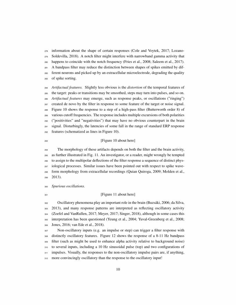
Artifactual features. Slightly less obvious is the distortion of the temporal features of284

the target: peaks or transitions may be smoothed, steps may turn into pulses, and so on.285

Artifactual features may emerge, such as response peaks, or oscillations (”ringing”)286

created de novo by the filter in response to some feature of the target or noise signal.287

Figure 10 shows the response to a step of a high-pass filter (Butterworth order 8) of288

various cutoff frequencies. The response includes multiple excursions of both polarities289

(”positivities” and ”negativities”) that may have no obvious counterpart in the brain290

signal. Disturbingly, the latencies of some fall in the range of standard ERP response291

features (schematized as lines in Figure 10).292


The morphology of these artifacts depends on both the filter and the brain activity,294

as further illustrated in Fig. 11. An investigator, or a reader, might wrongly be tempted295

to assign to the multipolar deflections of the filter response a sequence of distinct phys-296

iological processes. Similar issues have been pointed out with respect to spike wave-297

form morphology from extracellular recordings (Quian Quiroga, 2009; Molden et al.,298

2013).299

Spurious oscillations.300


Oscillatory phenomena play an important role in the brain (Buzsaki, 2006; da Silva,302

2013), and many response patterns are interpreted as reflecting oscillatory activity303

(Zoefel and VanRullen, 2017; Meyer, 2017; Singer, 2018), although in some cases this304

interpretation has been questioned (Yeung et al., 2004; Yuval-Greenberg et al., 2008;305

Jones, 2016; van Ede et al., 2018).306

Non-oscillatory inputs (e.g. an impulse or step) can trigger a filter response with307

distinctly oscillatory features. Figure 12 shows the response of a 8-11 Hz bandpass308

filter (such as might be used to enhance alpha activity relative to background noise)309

to several inputs, including a 10 Hz sinusoidal pulse (top) and two configurations of310

impulses. Visually, the responses to the non-oscillatory impulse pairs are, if anything,311

more convincingly oscillatory than the response to the oscillatory input!312

10


Oscillations tend to occur with a frequency close to a filter cutoff, and to be more314

salient for filters with a high order. They can occur for any filter with a sharp cutoff in315

the frequency domain, and are particularly salient for band-pass filters, as high-pass and316

low-pass cutoffs are close and may interact. Furthermore, if the pass band is narrow,317

the investigator might be tempted to choose a filter with steep cutoffs, resulting in a318

long impulse response with prolonged ringing.319

Masking or reintroduction of artifacts. Cognitive neuroscientists are alert to potential320

artifacts, for example muscular activity that differs between conditions due to different321

levels of effort. Muscular artifacts are most prominent in the gamma range (where322

they emerge from the 1/f background), and thus low-pass filtering is often indicated to323

eliminate them. Indeed, visually, there is little in the low-pass filtered signal to suggest324

muscle artifacts. Low-frequency correlates are nonetheless present (muscle spikes are325

wideband) and could potentially induce a statistically significant difference between326

conditions. Filtering masks this problem (if there is one).327

Conditions that require different levels of effort might also differ in the number of328

eye-blinks that they induce. Subjects are often encouraged to blink between trials, so as329

avoid contaminating data within the trials. However if high-pass or band-pass filtering330

is applied to the data before cutting them into epochs, the filter response to the blink331

may extend into the epoch, again inducing a statistically significant difference between332

conditions. For a causal filter each epoch is contaminated by any blinks that precede it,333

for an acausal filter it may also be contaminated by any blinks that follow it.334

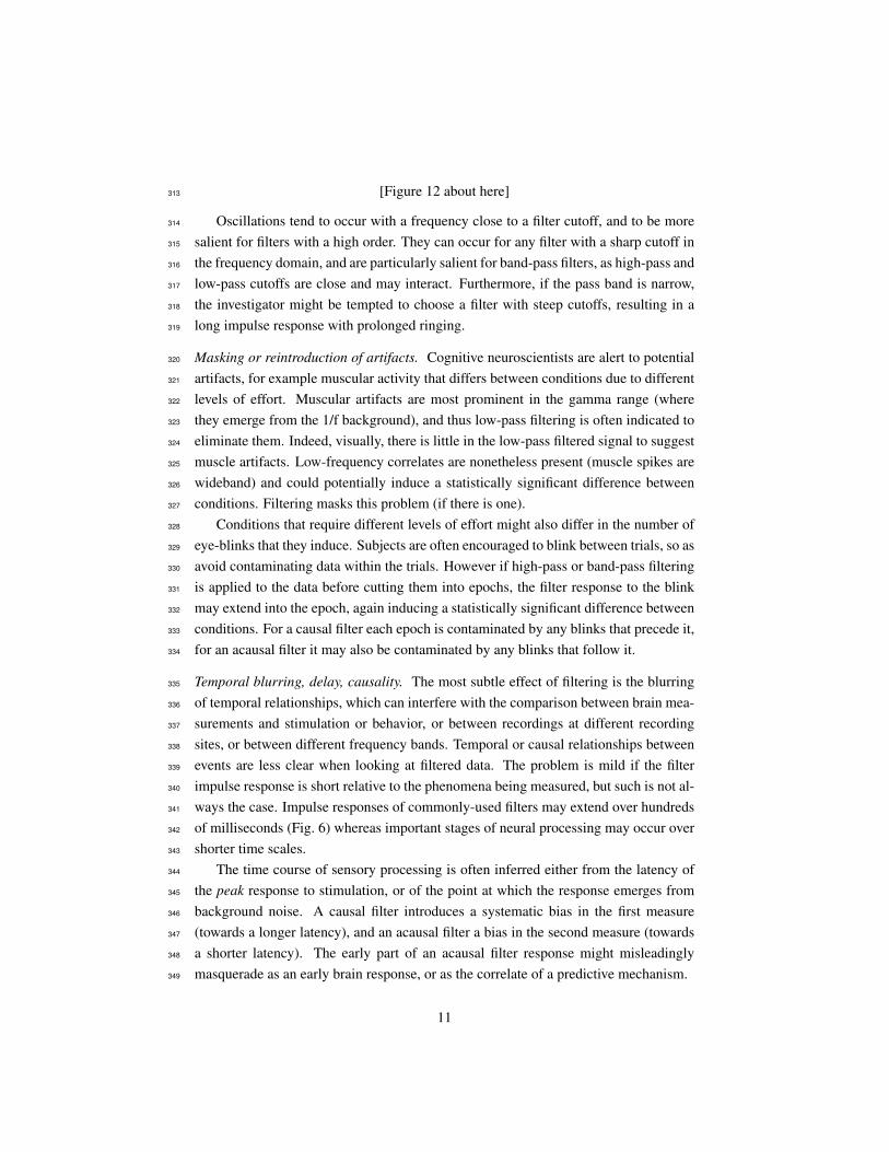
Temporal blurring, delay, causality. The most subtle effect of filtering is the blurring335

of temporal relationships, which can interfere with the comparison between brain mea-336

surements and stimulation or behavior, or between recordings at different recording337

sites, or between different frequency bands. Temporal or causal relationships between338

events are less clear when looking at filtered data. The problem is mild if the filter339

impulse response is short relative to the phenomena being measured, but such is not al-340

ways the case. Impulse responses of commonly-used filters may extend over hundreds341

of milliseconds (Fig. 6) whereas important stages of neural processing may occur over342

shorter time scales.343

The time course of sensory processing is often inferred either from the latency of344

the peak response to stimulation, or of the point at which the response emerges from345

background noise. A causal filter introduces a systematic bias in the first measure346

(towards a longer latency), and an acausal filter a bias in the second measure (towards347

a shorter latency). The early part of an acausal filter response might misleadingly348

masquerade as an early brain response, or as the correlate of a predictive mechanism.349

11

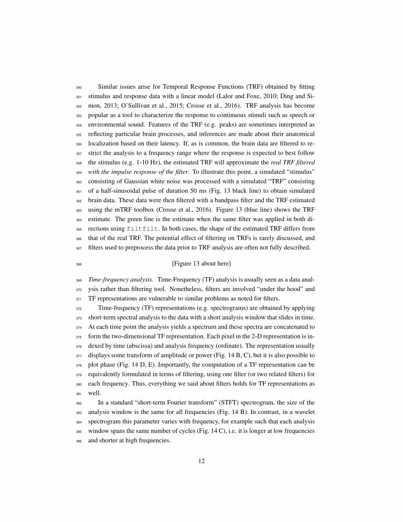
Similar issues arise for Temporal Response Functions (TRF) obtained by fitting350

stimulus and response data with a linear model (Lalor and Foxe, 2010; Ding and Si-351

mon, 2013; O’Sullivan et al., 2015; Crosse et al., 2016). TRF analysis has become352

popular as a tool to characterize the response to continuous stimuli such as speech or353

environmental sound. Features of the TRF (e.g. peaks) are sometimes interpreted as354

reflecting particular brain processes, and inferences are made about their anatomical355

localization based on their latency. If, as is common, the brain data are filtered to re-356

strict the analysis to a frequency range where the response is expected to best follow357

the stimulus (e.g. 1-10 Hz), the estimated TRF will approximate the real TRF filtered358

with the impulse response of the filter. To illustrate this point, a simulated “stimulus”359

consisting of Gaussian white noise was processed with a simulated “TRF” consisting360

of a half-sinusoidal pulse of duration 50 ms (Fig. 13 black line) to obtain simulated361

brain data. These data were then filtered with a bandpass filter and the TRF estimated362

using the mTRF toolbox (Crosse et al., 2016). Figure 13 (blue line) shows the TRF363

estimate. The green line is the estimate when the same filter was applied in both di-364

rections using filtfilt. In both cases, the shape of the estimated TRF differs from365

that of the real TRF. The potential effect of filtering on TRFs is rarely discussed, and366

filters used to preprocess the data prior to TRF analysis are often not fully described.367


Time-frequency analysis. Time-Frequency (TF) analysis is usually seen as a data anal-369

ysis rather than filtering tool. Nonetheless, filters are involved “under the hood” and370

TF representations are vulnerable to similar problems as noted for filters.371

Time-frequency (TF) representations (e.g. spectrograms) are obtained by applying372

short-term spectral analysis to the data with a short analysis window that slides in time.373

At each time point the analysis yields a spectrum and these spectra are concatenated to374

form the two-dimensional TF representation. Each pixel in the 2-D representation is in-375

dexed by time (abscissa) and analysis frequency (ordinate). The representation usually376

displays some transform of amplitude or power (Fig. 14 B, C), but it is also possible to377

plot phase (Fig. 14 D, E). Importantly, the computation of a TF representation can be378

equivalently formulated in terms of filtering, using one filter (or two related filters) for379

each frequency. Thus, everything we said about filters holds for TF representations as380

well.381

In a standard “short-term Fourier transform” (STFT) spectrogram, the size of the382

analysis window is the same for all frequencies (Fig. 14 B). In contrast, in a wavelet383

spectrogram this parameter varies with frequency, for example such that each analysis384

window spans the same number of cycles (Fig. 14 C), i.e. it is longer at low frequencies385

and shorter at high frequencies.386

12

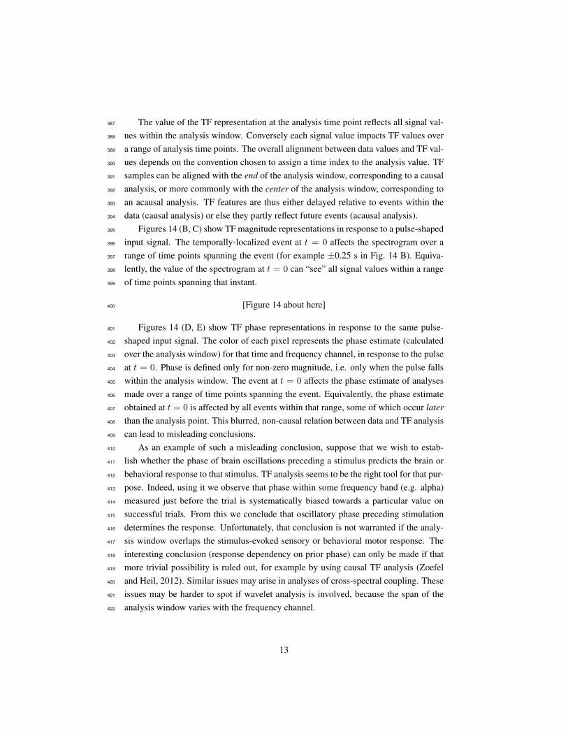
The value of the TF representation at the analysis time point reflects all signal val-387

ues within the analysis window. Conversely each signal value impacts TF values over388

a range of analysis time points. The overall alignment between data values and TF val-389

ues depends on the convention chosen to assign a time index to the analysis value. TF390

samples can be aligned with the end of the analysis window, corresponding to a causal391

analysis, or more commonly with the center of the analysis window, corresponding to392

an acausal analysis. TF features are thus either delayed relative to events within the393

data (causal analysis) or else they partly reflect future events (acausal analysis).394

Figures 14 (B, C) show TF magnitude representations in response to a pulse-shaped395

input signal. The temporally-localized event at t = 0 affects the spectrogram over a396

range of time points spanning the event (for example ±0.25 s in Fig. 14 B). Equiva-397

lently, the value of the spectrogram at t = 0 can “see” all signal values within a range398

of time points spanning that instant.399


Figures 14 (D, E) show TF phase representations in response to the same pulse-401

shaped input signal. The color of each pixel represents the phase estimate (calculated402

over the analysis window) for that time and frequency channel, in response to the pulse403

at t = 0. Phase is defined only for non-zero magnitude, i.e. only when the pulse falls404

within the analysis window. The event at t = 0 affects the phase estimate of analyses405

made over a range of time points spanning the event. Equivalently, the phase estimate406

obtained at t = 0 is affected by all events within that range, some of which occur later407

than the analysis point. This blurred, non-causal relation between data and TF analysis408

can lead to misleading conclusions.409

As an example of such a misleading conclusion, suppose that we wish to estab-410

lish whether the phase of brain oscillations preceding a stimulus predicts the brain or411

behavioral response to that stimulus. TF analysis seems to be the right tool for that pur-412

pose. Indeed, using it we observe that phase within some frequency band (e.g. alpha)413

measured just before the trial is systematically biased towards a particular value on414

successful trials. From this we conclude that oscillatory phase preceding stimulation415

determines the response. Unfortunately, that conclusion is not warranted if the analy-416

sis window overlaps the stimulus-evoked sensory or behavioral motor response. The417

interesting conclusion (response dependency on prior phase) can only be made if that418

more trivial possibility is ruled out, for example by using causal TF analysis (Zoefel419

and Heil, 2012). Similar issues may arise in analyses of cross-spectral coupling. These420

issues may be harder to spot if wavelet analysis is involved, because the span of the421

analysis window varies with the frequency channel.422

13

Notch filter artifacts. A narrow notch filter works well to remove narrowband interfer-423

ence that is stationary (e.g. 50 or 60 Hz line power). However, notch filtering may be424

less effective if the interference is not stationary. Amplitude fluctuations may occur if425

the subject moves, and for MEG the phase may fluctuate with changes in load in the426

tri-phase power network from which originates the interference. Artifacts can also be427

triggered by large-amplitude glitches (Kırac et al., 2015). Notch filtering is ineffective428

in removing interference close to the ends of the data (Fig. 9, bottom), and thus should429

not be applied to epoched data.430

Inadequate antialiasing.. Effects of the antialiasing filter are rarely noticed or objec-431

tionable. More serious may be a lack of sufficient antialiasing. Figure 15 (left) shows432

the power spectrum of a sample of data from a MEG system with shallow (or miss-433

ing) antialiasing. As common in MEG, there are salient power line components at 60434

Hz and harmonics (black arrows), but also many additional narrowband components435

that likely reflect aliasing of sources with frequencies beyond the Nyquist frequency436

(250 Hz). Possible sources include higher harmonics of 60 Hz, or high-frequency in-437

terference from computer screens, switching power supplies, etc. The frequency of the438

artifact cannot be known for sure. For example, the spectral line at 200 Hz (red arrow)439

could be the aliased 300 Hz harmonic of the power line interference, or it could have440

some other origin. This example underlines the importance of an adequate antialiasing441

filter.442

In contrast, Fig. 15 (left) shows the response to a sharp change in sensor state of443

one channel of a different MEG system with a particularly steep antialiasing filter (8th444

order elliptic filter with 120 dB rejection and 0.1 ripple in pass-band) (Oswal et al.,445

2016). The data show a prominent oscillatory pattern that is likely not present in the446

magnetic field measured by the device.447


6. How to fix it ?449

Report full filter specs. This should go without saying. In each case, the problem450

is compounded if the reader can’t form an opinion about possible effects of filtering.451

Filter type, order, frequency parameters, and whether it was applied in one direction or452

both (filtfilt) should be reported. Include a plot of the impulse response (and/or453

step response) as an inset to one of the plots. When reporting the order of a filter, be454

aware that for FIR filters this refers to the duration of the impulse response in samples455

(minus one), whereas for IIR filters implemented recursively it refers to the largest456

delay in the difference equation that produces each new output sample as a function of457

14

past input and output samples. The order of an IIR filter is usually small (e.g. 2-16),458

whereas that of an FIR is often large (e.g. 100-1000). The plot thickens when an IIR459

filter is approximated by an FIR filter. In that case, both numbers should be reported.460

An “order-512 Butterworth filter” is an unusual beast.461

Antialiasing artifacts.. Antialiasing artifacts are rarely an issue. In the event that they462

are, consider first whether antialiasing is needed. If you are certain that the original463

data contain no power beyond the Nyquist frequency, omit the filter and live danger-464

ously. If instead there are high-frequency sources of large amplitude, you might want465

to verify that the antialiasing filter attenuates them sufficiently before sampling. Note466

that, because of the aliasing, the frequency of those sources cannot be inferred with467

confidence from the sampled data. A wide-band oscilloscope or spectrum analyzer468

might be of use applied to the data before sampling. To reduce temporal smear and469

ringing, consider using an antialiasing filter with a lower cutoff and shallower slope. In470

the case of downsampling or resampling of a signal that is already sampled, consider471

alternatives such as interpolation (e.g. linear, cubic or spline). The artifact of Fig. 15472

(right) can be removed as described by de Cheveigne and Arzounian (2018).473

Low-pass. First, ask whether the aim is to smooth the temporal waveform, for example474

to enhance the clarity of a plot, or whether it is to ensure attenuation of high-frequency475

power (for example preceding downsampling). If the former, consider using a sim-476

ple smoothing kernel, for example square, triangular, or Gaussian (Fig. 6 a, b). Such477

kernels have a limited and well-defined temporal extent, and no negative portions so478

they do not produce ringing. They tend however to have poor spectral properties. Con-479

versely, if temporal distortion is of no importance, the filter can be optimized based480

only on its frequency response properties (Widmann et al., 2015).481

If data are recorded on multiple channels (e.g. local field potentials, EEG, or MEG),482

spatial filters may be applied to remove noise sources with a spatial signature different483

from the target sources. The appropriate filters can be found based on prior knowledge484

or using data-driven algorithms (e.g. Parra et al., 2005; de Cheveigne and Parra, 2014).485

High-pass. If the high-pass filter is required merely to remove a constant DC offset,486

consider subtracting the overall mean instead. If there is also a slow trend, consider de-487

trending rather than high-pass filtering. Detrending involves fitting a function (slowly-488

varying so as to fit the trend but not faster patterns) to the data and then subtracting the489

fit. Suitable functions include low-order polynomials. Like filtering, detrending is sen-490

sitive to temporally localized events such as glitches, however these can be addressed491

by robust detrending (de Cheveigne and Arzounian, 2018).492

15

If the slow trend signal can be estimated independently from the measurement that493

it contaminates, consider using regression techniques to factor it out (Vrba and Robin-494

son, 2001; de Cheveigne and Simon, 2007). Even when this is impossible, if the data495

are multichannel, consider using a component-analysis technique to factor it out, as has496

also been suggested to obtain distortion-free extracellular spike waveforms (Molden et497

al., 2013).498

If all else fails, and high-pass filtering must be used, pay particular attention to499

its possible effects on the morphology of responses. If the initial portion of the data500

(duration on the order of 1/fc where fc is the cutoff frequency) is on average far from501

zero, it may be useful to subtract the average over that portion, so as to minimize502

the filter response to the implicit initial step (the filter treats the input data as being503

preceded by zeros). If the data are to be cut into epochs (e.g. to excise responses to504

repeated stimuli), it is usually best to filter the continuous data first. Be aware that505

artifacts from out-of-epoch events (e.g. eye blinks) may extend to within the epoch.506

Band-pass. Consider whether a band-pass filter is really needed, as the potential for507

artifactual patterns is great. If band-pass filtering must be applied (for example to im-508

prove signal-to-noise ratio to assist a component-analysis technique), consider filters509

with relatively shallow slopes, and cutoff frequencies distant from the activity of inter-510

est. Be on the lookout for artifactual results due to the filtering.511

Notch. Notch filtering is usually motivated by the desire to suppress line noise (50512

Hz or 60 Hz and harmonics). Of course, the best approach is to eliminate that noise513

at the source by careful design of the setup, but this is not always feasible. As an514

alternative to filtering, it may be possible to measure the line noise on one or more515

reference channels and regress them out of the data (Vrba and Robinson, 2001). If516

the data are multichannel, consider using component analysis to isolate the line noise517

components and regress them out (Delorme et al., 2012; de Cheveigne and Parra, 2014;518

de Cheveigne and Arzounian, 2015).519

If the high-frequency region is not of interest, a simple expedient is to apply a520

boxcar smoothing kernel of size 1/50 Hz (or 1/60 Hz as appropriate). This simple521

low-pass filter has zeros at the line frequency and all its harmonics, and thus perfectly522

cancels line noise. The mild loss of temporal resolution (on the order of 20 ms) might523

be deemed acceptable. If the sampling rate differs from a multiple of the line frequency,524

the appropriate kernel can be implemented using interpolation (see de Cheveigne and525

Arzounian, 2018, for details).526

Time-frequency analysis. If the patterns of interest can be interpreted in the time do-527

main, eschew TF analysis. If the data are multichannel, and the aim is to increase the528

16

signal-to-noise ratio of narrow-band or stimulus-induced activity, consider component529

analysis techniques that can boost SNR of narrow-band signals (Nikulin et al., 2011;530

de Cheveigne and Arzounian, 2015).531

If TF analysis must be applied, consider using fixed kernel-size analysis (e.g. DFT)532

rather than, or in addition to, wavelet analysis, so that temporal bias and smearing are533

uniform across the frequency axis. Consider using relatively short analysis windows to534

reduce temporal bias and/or smearing. Weigh carefully the choice between causal anal-535

ysis (temporal bias but no causality issues) and acausal analysis (no temporal bias but536

risk of misleading causal relations). In every case, be alert for potential artifacts. One537

should be particularly concerned if an interesting effect only emerges with a particular538

analysis method.539

7. Horror scenarios540

This section imagines scenarios in which filtering effects might affect the science.541

Some are mildly embarrassing, others might keep a scientist awake at night.542

Missed observation.. Researcher A applies a high-pass filter to data recorded over a543

long period and fails to notice the existence of infra-slow brain activity (as reported by544

Vanhatalo et al., 2005). Researcher B applies a low-pass filter and fails to notice that a545

certain oscillatory activity is not sinusoidal (as reported by Cole and Voytek, 2017). It546

is frustrating to miss part of the phenomena one set out to study.547

Bias from eye movements.. Following a scenario hinted at in Sect. 5, researcher C548

runs a study in which some conditions are more demanding than others. Subjects are549

instructed to blink only between trials, but because acausal high-pass (or band-pass)550

filtering is applied to the data, each blink triggers a filter response that extends into the551

trial, resulting in a significant difference between conditions. Researcher D runs studies552

that create miniature eye movements (microsaccades) that differ between conditions.553

Microsaccades introduce so-called spike potentials, transients with a time course of554

a few tens of milliseconds, which after TF analysis boost energy in the gamma band555

selectively in some conditions rather than others (Yuval-Greenberg et al., 2008). In556

both cases ocular activity masquerades as brain activity.557

Distorted observation.. Researcher E records brain responses to stimulation, applies a558

high-pass filter to attenuate a pesky slow drift, and fails to notice that the brain response559

actually consisted of a sustained pedestal. Instead, a series of positive and negative560

peaks is observed and interpreted as reflecting a succession of processing stages in561

the brain. In a milder version of this scenario, the brain response does include such562

17

peaks, but the filter affects their position, leading to incorrect inferences concerning563

brain processing latencies.564

Flawed replication.. Researcher F replicates Researcher E’s experiments, using the565

same filters and generating the same artifacts. Results are consistent, giving weight to566

the conclusion that they are real.567

Faulty communication.. Researcher G, who is filter-savvy, reads his/her colleague’s568

papers and suspects something is amiss, but cannot draw firm conclusions because569

methods were not described in full. He/she re-runs the experiments with careful meth-570

ods, and finds results that invalidate the previous studies. The paper is not published571

because the study does not offer new results.572

Proliferation of “new” results.. Other researchers run further studies using analogous573

stimuli, but using different analysis parameters. New patterns of results are found that574

are interpreted as new discoveries, whereas the actual brain response (in this hypothet-575

ical scenario) is the same.576

Oscillations?. Researcher H knows that with the right kind of preprocessing, multiple577

layers of oscillatory activity can be found hidden within brain signals, and is confident578

that the analysis is revealing them. Researcher I suspects that these oscillations reflect579

filter ringing, but finds it hard to counter H’s arguments (Fourier’s theorem says that any580

signal is indeed a compound of oscillations). I remains worried because the observed581

oscillations depend on the choice of filter, but H is not: different filters extract different582

parts of the data, each with its own oscillatory nature. The debate mobilizes a good583

proportion of their energy.584

Biased time-frequency analysis.. Researcher K uses time-frequency analysis to test585

the hypothesis that the phase of ongoing brain oscillations modulates perceptual sen-586

sitivity. To avoid contamination by the sensory or behavioral response, the analysis is587

carefully restricted to the data preceding stimulation. However the analysis window,588

centered on the analysis point, extends far enough to include the sensory or behavioral589

response, biasing the distribution of measured phase. K concludes (incorrectly in this590

hypothetical scenario) that the hypothesis is correct. In a variant of this scenario, L uses591

time frequency analysis to test the hypothesis that brain activity is durably entrained by592

a rhythmical stimulus. The analysis is applied to the data beyond the stimulus offset,593

but the analysis window overlaps with the stimulus-evoked response, again biasing the594

phase distrtibution. L concludes (again incorrectly in this scenario) that the hypothesis595

was correct.596

18

8. Discussion597

A filter has one purpose, improve SNR, and two effects: improve SNR and distort598

the signal. Many investigators consider only the first and neglect the second. The599

filtered data are the sum of the filtered target signal and the filtered noise, and thus600

one can focus separately on these two effects (Fig. 16). Here we focused on target601

distortion.602


Issues related to distortion have been raised before, in particular distortion due to604

low-pass filtering (VanRullen, 2011; Rousselet, 2012; Widmann and Schroger, 2012),605

high-pass filtering (Kappenman and Luck, 2010; Acunzo et al., 2012; Tanner et al.,606

2015, 2016; Widmann et al., 2015; Lopez-Calderon and Luck, 2014) and band-pass607

filtering (Yeung et al., 2004), in the context of EEG and MEG and also extracellular608

recordings (Quian Quiroga, 2009; Molden et al., 2013; Yael and Bar-Gad, 2017). They609

are also discussed in textbooks and guidelines (Picton et al., 2000; Nunes and Srini-610

vasan, 2006; Gross et al., 2013; Keil et al., 2014; Luck, 2014; Puce and Hamalainen,611

2017; Cohen, 2014, 2017).612

How serious are these issues?. They can be recapitulated as follows. First, the loss of613

information in spectral regions suppressed by the filter. This problem is straightforward614

and does need elaboration. Second, the distortion of response waveforms and the emer-615

gence of spurious features. This is certainly a concern if spurious features (e.g. delayed616

excursions, or ringing) misleadingly suggest brain activity that is not there. Third, the617

blurring of temporal relations, in particular violation of causality. This too is a concern618

given the importance of response latency in inferring the sequence of neural events, or619

the anatomical stage at which they occur. Fourth, the non-uniqueness of phenomeno-620

logical descriptions: the same event can take very diverse shapes depending on the621

analysis. This can interfere with comparisons between studies, and can lead to redun-622

dant reports of the same phenomenon under different guise. Fifth, the lack of details623

required by a knowledgeable reader to infer the processing involved. Rather than an624

issue with filtering per se, the issue is with sloppy practice in reporting methodological625

details of filtering and TF analysis.626

Cutoff frequencies may be reported, but not the type of filter, its order, or whether627

it was applied in a single pass or both ways. As illustrated in Figs. 6 and 8, the cut-628

off frequency of a filter is not sufficient to characterize its impulse or step response,629

information that is needed to guess how it might have impacted a reported response.630

Failure to report details can be due to space limits (sometimes misguidedly imposed631

by journals), incomplete knowledge (e.g. proprietary or poorly documented software),632

19

reluctance to appear pedantic by reporting mundane trivia, or lack of understanding633

that this information is important.634

The issue of non-uniqueness is not often raised. Non-uniqueness refers to the fact635

that analysis of the same phenomenon can give rise to different descriptions depending636

on the analysis parameters, making it hard to compare across studies. It is sometimes637

recommended that parameters should be adjusted to the task at hand, rather than use de-638

fault values proposed by the software (Widmann and Schroger, 2012). Optimizing data639

analysis is laudable, but it carries the risks of “cherry-picking” or “double-dipping”640

(Kriegeskorte et al., 2009).641

Quid frequency and phase?. Filter design has developed sophisticated methods to op-642

timize the frequency response to maximize rejection, minimize ripple, and/or obtain643

the steepest possible transition between pass and stop bands. Engineers and scientists644

trained in those methods tend to choose a filter based on these properties, with less645

attention to their time-domain counterpart. It is not always clear that this emphasis is646

justified. For example, a band-pass filter with steep slopes might be motivated by the647

desire to “keep the delta band distinct from the theta band”, but given that there is little648

theoretical or phenomenological evidence for a clear boundary between bands, this is649

should perhaps not be a primary goal.650

For any given magnitude response, there are multiple filters with different phase651

responses. Of particular interest are zero phase filters with minimal waveform dis-652

tortion and no delay (but that are unfortunately acausal), and minimum phase filters653

with greater waveform distortion but that are causal. The choice between these phase654

characteristics (or others) depends on whether one wishes to favour causality, overall655

delay, or waveform distortion, knowing that it is impossible to favour all. Some authors656

recommend causal filters (Rousselet, 2012), others linear phase or acausal (Widmann657

and Schroger, 2012). Some studies report using simple filters (e.g. low order Butter-658

worth), others sophisticated designs (e.g. Chebyshev or elliptic) or even “brickwall”659

filters implemented in the Fourier domain.660

A crucial point that we strive to make in this paper is that no choice of filter can661

avoid temporal distortion, as any filter entails scrambling of the temporal axis (Fig. 2).662

Given that a filter with steep slopes in the frequency domain entails a long impulse re-663

sponse (a problem of particular importance when using brickwall filters in the Fourier664

domain), it may be worth relaxing spectral criteria so as to optimize temporal proper-665

ties.666

Causality, again.. As mentioned earlier, for an acausal filter the output depends on667

input values that occur later in the future. No physical system can have this behaviour.668

Offline analysis allows us greater flexibility to align the analysis arbitrarily with respect669

20

to the data, but we must be clear about what this implies. If we wish to relate the “brain670

response” to other events within the brain or the world (e.g. stimuli or behaviour),671

acausal filtering implies that that this response might depend on signal samples that672

occur after those events, indeed, a violation of causality.673

9. Recommendations674

Document.. This should go without saying, but many (most?) papers provide incom-675

plete information about the filters employed, a situation exacerbated by the insistence676

of some journals on limiting the space devoted to methods. Data analysis decisions,677

however suboptimal, can be justified, incomplete reporting cannot. The reader needs678

this information to infer the brain signal from the patterns reported.679

To authors: provide full specifications of the filters applied to the data. A simple680

plot of the impulse response (or step response) as an insert can be very helpful. To681

editors and reviewers: demand this information. To journals: avoid requirements that682

discourage proper documentation. To equipment manufacturers: provide full specifi-683

cations of any hardware filters.684

Know your filters.. Make sure that you know the exact filters that are involved in your685

data recording and analysis. This may require delving into the documentation (or even686

the code) of your analysis software (e.g. EEGlab, FieldTrip, SPM. etc.). Plot the im-687

pulse response and/or the step response and paste it on the wall in front of your desk.688

If several filters are cascaded, plot the response of their cascade. If specs are lack-689

ing, figure out how to deliver a pulse (and/or step) to the recording device and plot the690

resulting response. If you are using TF analysis, do you know exactly what kernels691

were employed? Are they causal and thus likely to introduce latency? Are they instead692

acausal (e.g. zero-phase) and thus likely to confuse causal relations? Are they wavelets,693

in which case temporal spread and latency might differ across frequency bands? All694

this should be known.695

Know your noise.. The main purpose of a filter is to attenuate noise. What is that696

noise, where does it come from? Might it be possible to mitigate it at the source? Some697

experimenters speak of their rig as if it were inhabited by gremlins. This deserves little698

patience: how can one understand the brain if we can’t find the source of line noise in699

the rig? It may not be possible to suppress the noise (e.g. turn off myogenic, cardiac,700

ocular or alpha activity, tramways in the street, etc.) but at least the source should be701

understood. Given that signal and noise both impact the results, understanding a noise702

process merits as much effort as understanding a brain process.703

21

Eliminate noise at the source.. No need for a filter if there is nothing to attenuate. To704

get rid of line noise: banish power cables from the vicinity of the setup, use lights fed705

with filtered DC, apply proper shielding (electrostatic coupling), avoid loops (magnetic706

coupling), avoid ground loops (ensure that ground cables and shields have a star topol-707

ogy with no loops), etc. To eliminate high-frequency noise: banish computer screens,708

fluorescent lights, equipment with switching power supplies, cell phones, etc. If need,709

apply Faraday shielding. To minimize slow drifts in EEG: follow appropriate proce-710

dures when applying the electrodes, and keep the subjects cool. To minimize alpha711

components: ensure that subjects keep their eyes open, give them a task to keep them712

alert, and so on. Textbooks (e.g. Luck, 2014; Cohen, 2014) and guidelines can offer713

many such suggestions.714

Ensure that you have adequate antialiasing.. Antialiasing filters in recording equip-715

ment are not always well documented. In some situations they might prove insufficient716

if there is high amplitude noise with a frequency beyond the Nyquist rate (for example717

from a computer screen, fluorescent light, or cell phone). A similar issue may arise718

when downsampling digital data: does the low-pass filter suffice to ensure that aliased719

components are negligible? This may require checking the data and/or software at hand720

(at the time of writing, Matlab’s resample sets the low-pass cutoff at Nyquist rather721

than below, which is inadequate).722

Consider alternatives to filtering.. Consider detrending (in particular robust detrend-723

ing) as an alternative to high-pass filtering (Bigdely-Shamlo et al., 2015; de Cheveigne724

and Arzounian, 2018). Consider using an independent reference signal measurement725

that picks up only noise, and use regression techniques to factor out the noise (Vrba726

and Robinson, 2001; de Cheveigne and Simon, 2007; Molden et al., 2013). Consider727

component analysis techniques to design a spatial filter that factors out the noise (Parra728

et al., 2005; Delorme et al., 2012; de Cheveigne and Parra, 2014).729

Choose the right filter.. If filter we must, a prime consideration is whether to opti-730

mize the time domain (minimal distortion of the waveform) or the frequency domain731

(optimal frequency response), the two being at loggerheads. Taking the example of a732

low-pass filter, if our goal is to smooth the waveform to enhance the visual clarity of a733

plot, or locate a peak with less jitter, then a simple box-car smoothing kernel (rectan-734

gular impulse response) may be sufficient, with minimal temporal blurring. The poor735

frequency response of such a low-pass filter is of little import. If instead the focus is on736

spectral features (e.g. frequency-following response, or narrowband oscillations), we737

may wish to optimize the spectral properties of the filter at the expense of greater tem-738

poral smearing. If the focus is on spectrotemporal features, then the choice of filter(s)739

necessarily involves a tradeoff between the two (Cohen, 2014).740

22

Simulate.. It is hard to fully predict the impact of filtering, particularly if multiple741

stages are cascaded. A simple expedient is to simulate the situation using a known742

target signal (e.g. an idealized evoked response) and known noise (e.g. EEG data from743

an unrelated recording). The effect of filtering can then be evaluated separately on744

each, given that the filtered sum is the sum of the filtered parts (Fig. 16).745

The synthetic target signal could be an impulse or step (to visualize canonical re-746

sponse properties), or a signal similar to a typically-observed response (to see how747

processing might affect it), or a signal constructed to mimic the observed response af-748

ter filtering (to help infer true patterns from observations). Observing the response to749

the target tells us how it is distorted, observing the response to the noise tells us how750

well it is attenuated and what artifactual patterns to expect. Comparing the two tells us751

whether our observation is helped (or hindered) by filtering.752

Be paranoid.. Is the effect of interest only visible for a particular type of filter, or a753

particular variety of TF analysis? Consider whether it might depend on an artifact of754

that filter or analysis. Do your conclusions involve temporal or causal dependencies be-755

tween events in the EEG and events in the world? Make sure that you fully understand756

how they might be affected by filtering or the TF analysis.757

Go with the zeitgeist.. This is in counterpoint to the previous recommendations. One758

cannot ignore that many studies, past and present, employ filters in ways that we de-759

scribe as problematic. Those results cannot be discarded, and one may need to use760

similar methods oneself to allow comparisons, and place new results within the context761

of prior knowledge. Many researchers and laboratories have well established method-762

ologies that may need to be adhered to for consistency. If such is the case, go for it, but763

don’t forget to fully document, and do call the reader’s attention to potential issues.764

Conclusion765

Filters are ubiquitous in electrophysiology and neuroscience and are an important766

part of the methodology of any study. Their role is to suppress noise and enhance target767

activity, but they may have deleterious effects that the investigator should be aware of.768

When reporting results, it is important to provide enough details so that the reader too769

can be aware of these potential effects. In some cases there exist alternatives to filtering770

that are worth considering, in others a filter cannot be avoided. In every case, care must771

taken to fully understand and report the potential effects of filtering on the patterns772

reported.773

23

Acknowledgements774

The first author was supported by the EU H2020-ICT grant 644732 (COCOHA),775

and grants ANR-10-LABX-0087 IEC and ANR-10-IDEX-0001-02 PSL*. The second776

author was supported by grant 390/12 from the Israel Science Foundation (ISF) and by777

ERC advanced grant GA-340063 (project RATLAND). Giovanni Di Liberto offered778

useful comments on previous manuscripts.779

Author Contributions780

Conceptualization and writing: AdC and IN.781

Declaration of Interests782

None.783

References784

Acunzo DJ, MacKenzie G, van Rossum MCW (2012) Systematic biases in early ERP785

and ERF components as a result of high-pass filtering. Journal of Neuroscience786

Methods 209:212–218.787

Bigdely-Shamlo N, Mullen T, Kothe C, Su KM, Robbins KA (2015) The PREP788

pipeline: standardized preprocessing for large-scale EEG analysis. Frontiers in Neu-789

roinformatics 9:16.790

Buzsaki G (2006) Rhythms Of The Brain Oxford Univ. Press.791

Cohen MX (2017) Rigor and replication in time-frequency analyses of cognitive elec-792

trophysiology data. International Journal of Psychophysiology 111:80–87.793

Cohen MX (2014) Analyzing Neural Time Series Data - Theory and practice MIT794

Press.795

Cole SR, Voytek B (2017) Brain Oscillations and the Importance of Waveform Shape.796

Trends in Cognitive Sciences 21:137–149.797

Crosse MJ, Di Liberto GM, Bednar A, Lalor EC (2016) The Multivariate Tempo-798

ral Response Function (mTRF) Toolbox: A MATLAB Toolbox for Relating Neural799

Signals to Continuous Stimuli. Frontiers in Human Neuroscience 10:1–14.800

da Silva FL (2013) EEG and MEG: Relevance to Neuroscience. Neuron 80:1112–1128.801

24

de Cheveigne A, Arzounian D (2015) Scanning for oscillations. Journal of Neural802

Engineering 12:66020.803

de Cheveigne A, Arzounian D (2018) Robust detrending, rereferencing, outilier detec-804

tion, and inpainting of multichannel data. NeuroImage 172:903–912.805

de Cheveigne A, Parra LC (2014) Joint decorrelation, a versatile tool for multichannel806

data analysis. NeuroImage 98:487–505.807

de Cheveigne A, Simon JZ (2007) Denoising based on time-shift PCA. Journal of808

Neuroscience Methods 165:297–305.809

Delorme A, Palmer J, Onton J, Oostenveld R, Makeig S (2012) Independent EEG810

sources are dipolar. PLoS ONE 7:e30135.811

Ding N, Simon JZ (2013) Adaptive Temporal Encoding Leads to a812

Background-Insensitive Cortical Representation of Speech. Journal of Neuro-813

science 33:5728–5735.814

Fries P, Scheeringa R, Oostenveld R (2008) Finding Gamma. Neuron 58:303–305.815

Gross J, Baillet S, Barnes GR, Henson RN, Hillebrand A, Jensen O, Jerbi K, Litvak816

V, Maess B, Oostenveld R, Parkkonen L, Taylor JR, van Wassenhove V, Wibral M,817

Schoffelen JM (2013) Good practice for conducting and reporting MEG research.818

NeuroImage 65:349–363.819

Huigen E, Peper a, Grimbergen Ca (2002) Investigation into the origin of the noise of820

surface electrodes. Medical & biological engineering & computing 40:332–338.821

Jones SR (2016) When brain rhythms aren’t rhythmic’: implication for their mecha-822

nisms and meaning. Current Opinion in Neurobiology 40:72–80.823

Kappenman ES, Luck SJ (2010) The effects of electrode impedance on data quality824

and statistical significance in ERP recordings. Psychophysiology 47:888–904.825

Keil A, Debener S, Gratton G, Junghofer M, Kappenman ES, Luck SJ, Luu P, Miller826

GA, Yee CM (2014) Committee report: Publication guidelines and recommenda-827

tions for studies using electroencephalography and magnetoencephalography. Psy-828

chophysiology 51:1–21.829

Kırac L, Vollmar C, Remi J, Loesch A, Noachtar S (2015) Notch filter artefact mim-830

icking high frequency oscillation in epilepsy. Clinical Neurophysiology 127.831

25

Kriegeskorte N, Simmons WK, Bellgowan PSF, Baker CI (2009) Circular anal-832

ysis in systems neuroscience: the dangers of double dipping. Nature Neuro-833

science 12:535–540.834

Lalor EC, Foxe JJ (2010) Neural responses to uninterrupted natural speech can835

be extracted with precise temporal resolution. European Journal of Neuro-836

science 31:189–193.837

Lammertmann C, Lutkenhoner B (2001) Near-DC magnetic fields following a periodic838

presentation of long-duration tonebursts. Clinical Neurophysiology 112:499–513.839

Lopez-Calderon J, Luck SJ (2014) ERPLAB: an open-source toolbox for the analysis840

of event-related potentials. Frontiers in Human Neuroscience 8:1–14.841

Lozano-Soldevilla D (2018) Nonsinusoidal neuronal oscillations: bug or feature? Jour-842

nal of Neurophysiology 119:1595–1598.843

Luck S (2014) An introduction to the event-related potential technique MIT press.844

Meyer L (2017) The neural oscillations of speech processing and language compre-845

hension: State of the art and emerging mechanisms. European Journal of Neuro-846

science 48:2609–2621.847

Molden S, Moldestad O, Storm JF (2013) Estimating extracellular spike waveforms848

from CA1 pyramidal cells with multichannel electrodes. PLoS ONE 8.849

Nikulin VV, Nolte G, Curio G (2011) A novel method for reliable and fast extraction850

of neuronal EEG/MEG oscillations on the basis of spatio-spectral decomposition.851

NeuroImage 55:1528–1535.852

Nunes P, Srinivasan R (2006) Electric Fields of the Brain: The Neurophysics of EEG853

Oxford University Press.854

O’Sullivan JA, Shamma SA, Lalor EC (2015) Evidence for Neural Computations of855

Temporal Coherence in an Auditory Scene and Their Enhancement during Active856

Listening. Journal of Neuroscience 35:7256–7263.857

Oswal A, Jha A, Neal S, Reid A, Bradbury D, Aston P, Limousin P, Foltynie T, Zrinzo858

L, Brown P, Litvak V (2016) Analysis of simultaneous MEG and intracranial LFP859

recordings during Deep Brain Stimulation: A protocol and experimental validation.860

Journal of Neuroscience Methods 261:29–46.861

Parra LC, Spence CD, Gerson AD, Sajda P (2005) Recipes for the linear analysis of862

EEG. Neuroimage 28:326–341.863

26

Picton TW, Bentin S, Berg P, Donchin E, Hillyard SA, Johnson R, Miller GA, Ritter864

W, Ruchkin DS, Rugg MD, Taylor MJ (2000) Guidelines for using human event-865

related potentials to study cognition: recording standards and publication criteria.866

Psychophysiology 37:127–152.867

Picton TW, Woods DL, Proulx GB (1978) Human auditory sustained potentials. I.868

The nature of the response. Electroencephalography and Clinical Neurophysiol-869

ogy 45:186–197.870

Puce A, Hamalainen MS (2017) A review of issues related to data acquisition and871

analysis in EEG/MEG studies. Brain Sciences 7.872

Quian Quiroga R (2009) What is the real shape of extracellular spikes? Journal of873

Neuroscience Methods 177:194–198.874

Rousselet GA (2012) Does filtering preclude us from studying ERP time-courses?875

Frontiers in Psychology 3:1–9.876

Saleem AB, Lien AD, Krumin M, Haider B, Roson MR, Ayaz A, Reinhold K, Busse L,877

Carandini M, Harris KD, Carandini M (2017) Subcortical Source and Modulation of878

the Narrowband Gamma Oscillation in Mouse Visual Cortex. Neuron 93:315–322.879

Singer W (2018) Neuronal oscillations: Unavoidable and useful? European Journal880

of Neuroscience 48:2389–2398.881

Southwell R, Baumann A, Gal C, Barascud N, Friston K, Chait M (2017) Is882

predictability salient? a study of attentional capture by auditory patterns.883

Philosophical Transactions of the Royal Society of London B: Biological Sci-884

ences 372:doi:10.1098/rstb.2016.0105.885

Tanner D, Morgan-Short K, Luck SJ (2015) How inappropriate high-pass filters can886

produce artifactual effects and incorrect conclusions in ERP studies of language and887

cognition. Psychophysiology 52:997–1009.888

Tanner D, Norton JJ, Morgan-Short K, Luck SJ (2016) On high-pass filter artifacts889

(they’re real) and baseline correction (it’s a good idea) in ERP/ERMF analysis. Jour-890

nal of Neuroscience Methods 266:166–170.891

van Ede F, Quinn AJ, Woolrich MW, Nobre AC (2018) Neural Oscillations: Sustained892

Rhythms or Transient Burst-Events? Trends in Neurosciences 41:415–417.893

Vanhatalo S, Voipio J, Kaila K (2005) Full-band EEG (FbEEG): An emerging standard894

in electroencephalography. Clinical Neurophysiology 116:1–8.895

27

VanRullen R (2011) Four common conceptual fallacies in mapping the time course of896

recognition. Frontiers in Psychology 2:1–6.897

Vrba J, Robinson SE (2001) Signal Processing in Magnetoencephalography. Meth-898

ods 25:249–271.899

Widmann A, Schroger E (2012) Filter effects and filter artifacts in the analysis of900

electrophysiological data. Frontiers in Psychology 3:1–5.901

Widmann A, Schroger E, Maess B (2015) Digital filter design for electrophysiological902

data - a practical approach. Journal of Neuroscience Methods 250:34–46.903

Yael D, Bar-Gad I (2017) Filter based phase distortions in extracellular spikes. PLoS904

ONE 12:1–13.905

Yeung N, Bogacz R, Holroyd CB, Cohen JD (2004) Detection of synchronized os-906

cillations in the electroencephalogram: An evaluation of methods. Psychophysiol-907

ogy 41:822–832.908

Yuval-Greenberg S, Tomer O, Keren AS, Nelken I, Deouell LY (2008) Transient In-909

duced Gamma-Band Response in EEG as a Manifestation of Miniature Saccades.910

Neuron 58:429–441.911

Zoefel B, Heil P (2012) Detection of Near-Threshold Sounds is Independent of EEG912

Phase in Common Frequency Bands. Frontiers in Psychology 4:262.913

Zoefel B, VanRullen R (2017) Oscillatory mechanisms of stimulus processing and914

selection in the visual and auditory systems: State-of-the-art, speculations and sug-915

gestions. Frontiers in Neuroscience 11:1–13.916

28

Captions917

Figure 1: A typical recording-to-publication data pipeline, showing where filters are ap-plied. Filters are analog in the first stages (green) and digitial in subsequent stages (red).The recording rig might include a high-pass filter (implicit in the case of AC coupling), andperhaps also a notch filter to attenuate line frequency power. The analog-to-digital con-verter is preceded by a low-pass antialiasing filter. In data preprocessing it is common toapply a high-pass filter to remove slow drift components, and a low-pass filter to attenuatenoise (often spread over the entire spectrum), or to avoid antialiasing when the data aredown-sampled. Data analysis might involve bandpass filtering (for example to isolate astandard frequency band such as ”alpha” or ”gamma”) or time-frequency analysis. Datadisplay or plotting might call for additional smoothing (low-pass filtering).

Figure 2: Filtering. Top: each sample of the output y is the sum of samples of the input xweighted by the impulse response h. For a causal filter, only past or present samples of theinput make a contribution (black). For an acausal filter, future samples too can contribute(gray). Bottom: another way of describing this process is that each sample of the input xaffects multiple samples of the output y, with a weight determined by the impulse responseh.

Figure 3: Typical magnitude transfer function shapes (top) and the associated impulse re-sponses (bottom). The low-pass filter attenuates high frequencies, the high-pass attenuateslow frequencies, the band-pass attenuates out-of band frequencies, the notch attenuates anarrow band of freqencies. The steeper the transition in the frequency domain, the moreextended the impulse response (red). The steepness of the transitions depends on the typeand order of the filter. Low-pass, high-pass and band-pass are Butterworth filters of or-der 4 and 16, notch filters are second-order filters with Q factors (ratio of bandwidth tocentre frequency) of 1 and 10. Impulse responses for high-pass and notch include a highamplitude impulse, plotted here with a break.

29

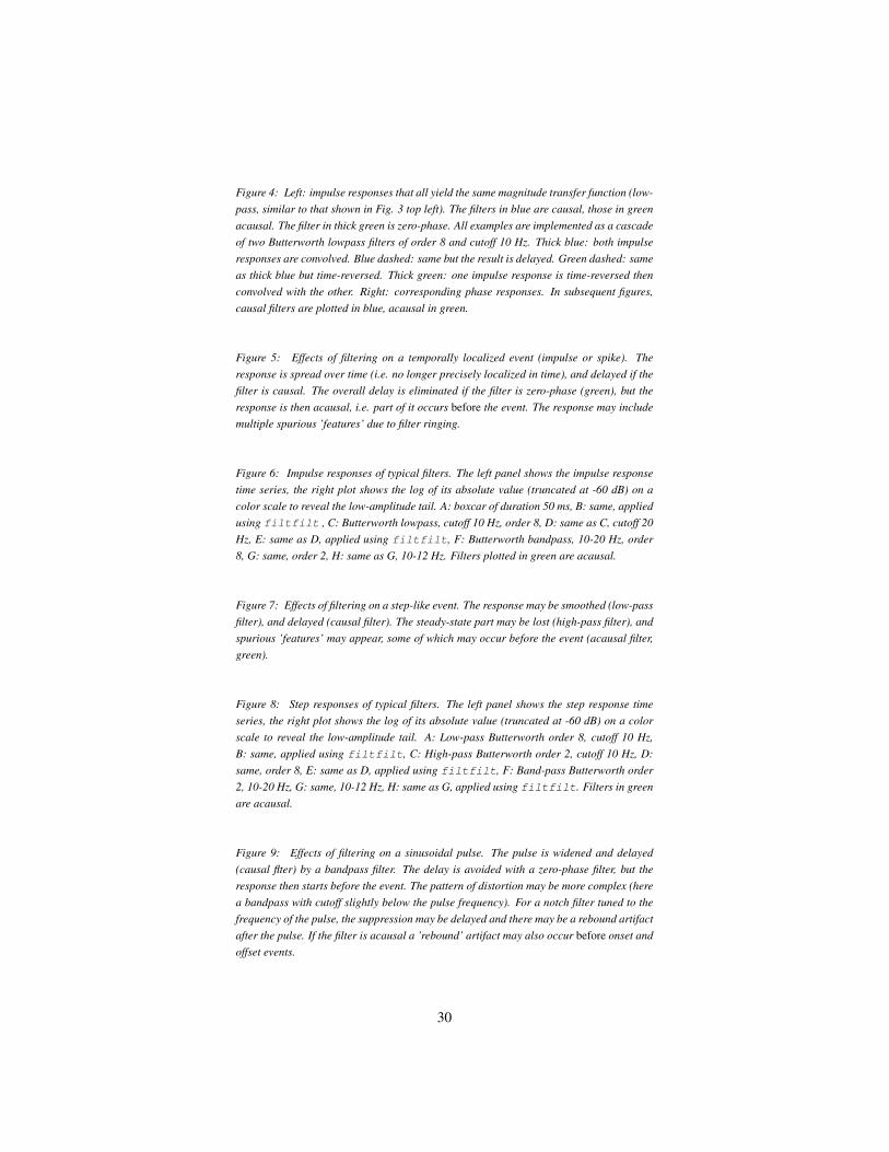
Figure 4: Left: impulse responses that all yield the same magnitude transfer function (low-pass, similar to that shown in Fig. 3 top left). The filters in blue are causal, those in greenacausal. The filter in thick green is zero-phase. All examples are implemented as a cascadeof two Butterworth lowpass filters of order 8 and cutoff 10 Hz. Thick blue: both impulseresponses are convolved. Blue dashed: same but the result is delayed. Green dashed: sameas thick blue but time-reversed. Thick green: one impulse response is time-reversed thenconvolved with the other. Right: corresponding phase responses. In subsequent figures,causal filters are plotted in blue, acausal in green.

Figure 5: Effects of filtering on a temporally localized event (impulse or spike). Theresponse is spread over time (i.e. no longer precisely localized in time), and delayed if thefilter is causal. The overall delay is eliminated if the filter is zero-phase (green), but theresponse is then acausal, i.e. part of it occurs before the event. The response may includemultiple spurious ’features’ due to filter ringing.

Figure 6: Impulse responses of typical filters. The left panel shows the impulse responsetime series, the right plot shows the log of its absolute value (truncated at -60 dB) on acolor scale to reveal the low-amplitude tail. A: boxcar of duration 50 ms, B: same, appliedusing filtfilt , C: Butterworth lowpass, cutoff 10 Hz, order 8, D: same as C, cutoff 20Hz, E: same as D, applied using filtfilt, F: Butterworth bandpass, 10-20 Hz, order8, G: same, order 2, H: same as G, 10-12 Hz. Filters plotted in green are acausal.

Figure 7: Effects of filtering on a step-like event. The response may be smoothed (low-passfilter), and delayed (causal filter). The steady-state part may be lost (high-pass filter), andspurious ’features’ may appear, some of which may occur before the event (acausal filter,green).

Figure 8: Step responses of typical filters. The left panel shows the step response timeseries, the right plot shows the log of its absolute value (truncated at -60 dB) on a colorscale to reveal the low-amplitude tail. A: Low-pass Butterworth order 8, cutoff 10 Hz,B: same, applied using filtfilt, C: High-pass Butterworth order 2, cutoff 10 Hz, D:same, order 8, E: same as D, applied using filtfilt, F: Band-pass Butterworth order2, 10-20 Hz, G: same, 10-12 Hz, H: same as G, applied using filtfilt. Filters in greenare acausal.

Figure 9: Effects of filtering on a sinusoidal pulse. The pulse is widened and delayed(causal flter) by a bandpass filter. The delay is avoided with a zero-phase filter, but theresponse then starts before the event. The pattern of distortion may be more complex (herea bandpass with cutoff slightly below the pulse frequency). For a notch filter tuned to thefrequency of the pulse, the suppression may be delayed and there may be a rebound artifactafter the pulse. If the filter is acausal a ’rebound’ artifact may also occur before onset andoffset events.

30

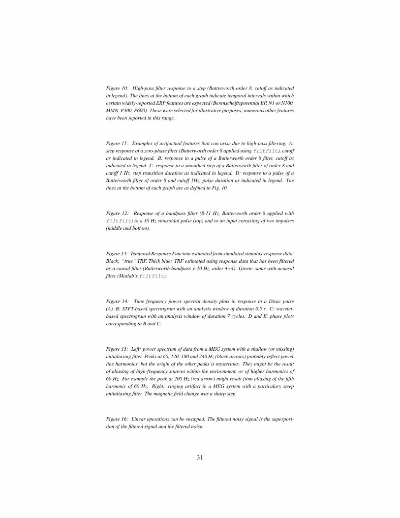
Figure 10: High-pass filter response to a step (Butterworth order 8, cutoff as indicatedin legend). The lines at the bottom of each graph indicate temporal intervals within whichcertain widely-reported ERP features are expected (Berenscheiftspotential BP, N1 or N100,MMN, P300, P600). These were selected for illustrative purposes; numerous other featureshave been reported in this range.

Figure 11: Examples of artifactual features that can arise due to high-pass filtering. A:step response of a zero-phase filter (Butterworth order 8 applied using filtfilt), cutoffas indicated in legend. B: response to a pulse of a Butterworth order 8 filter, cutoff asindicated in legend. C: response to a smoothed step of a Butterworth filter of order 8 andcutoff 1 Hz, step transition duration as indicated in legend. D: response to a pulse of aButterworth filter of order 8 and cutoff 1Hz, pulse duration as indicated in legend. Thelines at the bottom of each graph are as defined in Fig. 10.

Figure 12: Response of a bandpass filter (8-11 Hz, Butterworth order 8 applied withfiltfilt) to a 10 Hz sinusoidal pulse (top) and to an input consisting of two impulses(middle and bottom).

Figure 13: Temporal Response Function estimated from simulated stimulus-response data.Black: “true” TRF. Thick blue: TRF estimated using response data that has been filteredby a causal filter (Butterworth bandpass 1-10 Hz, order 4+4). Green: same with acausalfilter (Matlab’s filtfilt).

Figure 14: Time frequency power spectral density plots in response to a Dirac pulse(A). B: STFT-based spectrogram with an analysis window of duration 0.5 s. C: wavelet-based spectrogram with an analysis window of duration 7 cycles. D and E: phase plotscorresponding to B and C.

Figure 15: Left: power spectrum of data from a MEG system with a shallow (or missing)antialiasing filter. Peaks at 60, 120, 180 and 240 Hz (black arrows) probably reflect powerline harmonics, but the origin of the other peaks is mysterious. They might be the resultof aliasing of high-frequency sources within the environment, or of higher harmonics of60 Hz. For example the peak at 200 Hz (red arrow) might result from aliasing of the fifthharmonic of 60 Hz. Right: ringing artifact in a MEG system with a particulary steepantialiasing filter. The magnetic field change was a sharp step.

Figure 16: Linear operations can be swapped. The filtered noisy signal is the superposi-tion of the filtered signal and the filtered noise.

31

Documents

Filters: When, Why, and How (Not) to Use Them