Embed Size (px)
Citation preview

EECS 247 Lecture 2: Filters © © 2005 H.K. Page 1
EE247 - Lecture 2Filters
• Material covered today:– Nomenclature– Filter specifications
• Quality factor• Frequency characteristics• Group delay
– Filter types• Butterworth• Chebyshev I• Chebyshev II• Elliptic• Bessel
– Group delay comparison example
EECS 247 Lecture 2: Filters © © 2005 H.K. Page 2
Filters
Filtersà Provide frequency selectivity and/or phase shaping
inV
FilteroutV
( )ωjH
ωω
( )ωjH

EECS 247 Lecture 2: Filters © © 2005 H.K. Page 3
NomenclatureFilter Types
( )ωjH( )ωjH
Lowpass Highpass Bandpass Band-reject(Notch)
ω ω ω
Provide frequency selectivity
( )ωjH( )ωjH
ω ω
All-pass
( )ωjH
Phase shaping or equalization
EECS 247 Lecture 2: Filters © © 2005 H.K. Page 4
Filter Specifications
• Frequency characteristics (lowpass filter):– Passband ripple (Rpass)– Cutoff frequency or -3dB frequency – Stopband rejection– Passband gain
• Phase characteristics:– Group delay
• SNR (Dynamic range)• SNDR (Signal to Noise+Distortion ratio)• Linearity measures: IM3 (intermodulation distortion), HD3
(harmonic distortion), IIP3 or OIP3 (Input-referred or output-referred third order intercept point)
• Power/pole & Area/pole

EECS 247 Lecture 2: Filters © © 2005 H.K. Page 5
0
x 10Frequency (Hz)
Lowpass Filter Frequency Characteristics
( )ωjH
( )ωjH
( )0H
Passband Ripple (Rpass)
Transition Band
cfPassband
Passband Gain
stopfStopband Frequency
Stopband Rejection
f
( )ωjH3dBf−
dB3
EECS 247 Lecture 2: Filters © © 2005 H.K. Page 6
Quality Factor (Q)
• The term Quality Factor (Q) has different definitions:– Component quality factor (inductor & capacitor
Q)– Pole quality factor– Bandpass filter quality factor
• Next 3 slides clarifies each
EECS 247 Lecture 2: Filters © © 2005 H.K. Page 7
Component Quality Factor (Q)
• For any component with a transfer function:
• Quality factor is defined as:
( ) ( ) ( )
( )( )
Energy StoredAverage Power Dissipat ion
1H jR jX
XQ
R
ω ω ω
ωω →
= +
=
EECS 247 Lecture 2: Filters © © 2005 H.K. Page 8
Inductor & Capacitor Quality Factor
• Inductor Q :
• Capacitor Q :
Rs LL L1 LY QRs j L Rs
ωω= =+
Rp
CC C
1Z Q CRp1 jRp Cω
ω= =
+

EECS 247 Lecture 2: Filters © © 2005 H.K. Page 9
Pole Quality Factor
xσ
xω
ωj
σ
Pω
xPole
xQ
2ωσ
=
s-Plane
EECS 247 Lecture 2: Filters © © 2005 H.K. Page 10
Bandpass Filter Quality Factor (Q)
-2 0
-15
-10
-5
0
0.1 1 10f1 fcenter f2
0
-3dB
∆f = f2 - f1
( )H jf
Frequency
Mag
nitu
de (d
B)
Q= fcenter /∆f

EECS 247 Lecture 2: Filters © © 2005 H.K. Page 11
• Consider a continuous time filter with s-domain transfer function G(s):
• Let us apply a signal to the filter input composed of sum of twosinewaves at slightly different frequencies (∆ω<<ω):
• The filter output is:
What is Group Delay?
vIN(t) = A1sin(ωt) + A2sin[(ω+∆ω) t]
G(jω) ≡ G(jω)ejθ(ω)
vOUT(t) = A1 G(jω) sin[ωt+θ(ω)] +
A2 G[ j(ω+∆ω)] sin[(ω+∆ω)t+ θ(ω+∆ω)]
EECS 247 Lecture 2: Filters © © 2005 H.K. Page 12
What is Group Delay?
{ ]}[vOUT(t) = A1 G(jω) sin ω t + θ(ω)
ω +
{ ]}[+ A2 G[ j(ω+∆ω)] sin (ω+∆ω) t + θ(ω+∆ω)ω+∆ω
θ(ω+∆ω)ω+∆ω ≅ θ(ω)+
dθ(ω)dω
∆ω[ ][ 1ω )( ]1 -
∆ωω
dθ(ω)dω
θ(ω)ω +
θ(ω)ω-( ) ∆ω
ω≅
∆ωω <<1Since then ∆ω
ω à0[ ]2

EECS 247 Lecture 2: Filters © © 2005 H.K. Page 13
What is Group Delay?Signal Magnitude and Phase Impairment
{ ]}[vOUT(t) = A1 G(jω) sin ω t + θ(ω)
ω +
{ ]}[+ A2 G[ j(ω+∆ω)]sin (ω+∆ω) t +dθ(ω)
dωθ(ω)
ω +θ(ω)
ω-( )∆ωω
• If the second term in the phase of the 2nd sin wave is non-zero, then the filter’s output at frequency ω+∆ω is time-shifted differently than the filter’s output at frequency ωà “Phase distortion”
• If the second term is zero, then the filter’s output at frequency ω+∆ωand the output at frequency ω are each delayed in time by -θ(ω)/ω
• τPD ≡ -θ(ω)/ω is called the “phase delay” and has units of time
EECS 247 Lecture 2: Filters © © 2005 H.K. Page 14
• Phase distortion is avoided only if:
• Clearly, if θ(ω)=kω, k a constant, à no phase distortion• This type of filter phase response is called “linear phase”
àPhase shift varies linearly with frequency• τGR ≡ -dθ(ω)/dω is called the “group delay” and also has units
of time. For a linear phase filter τGR ≡ τPD =k à τGR= τPD implies linear phase
• Note: Filters with θ(ω)=kω+c are also called linear phase filters, but they’re not free of phase distortion
What is Group Delay?Signal Magnitude and Phase Impairment
dθ(ω)dω
θ(ω)ω- = 0

EECS 247 Lecture 2: Filters © © 2005 H.K. Page 15
What is Group Delay?Signal Magnitude and Phase Impairment
• If τGR= τPDà No phase distortion
[ )](vOUT(t) = A1 G(jω) sin ω t - τGR +
[+ A2 G[ j(ω+∆ω)] sin (ω+∆ω) )]( t - τGR
• If alsoG( jω)=G[ j(ω+∆ω)] for all input frequencies within the signal-band, vOUT is a scaled, time-shifted replica of the input, with no “signal magnitude distortion” :
• In most cases neither of these conditions are realizable exactly
EECS 247 Lecture 2: Filters © © 2005 H.K. Page 16
• Phase delay is defined as:τPD ≡ -θ(ω)/ω [ time]
• Group delay is defined as :τGR ≡ -dθ(ω)/dω [time]
• If θ(ω)=kω, k a constant, à no phase distortion
• For a linear phase filter τGR ≡ τPD =k
SummaryGroup Delay

EECS 247 Lecture 2: Filters © © 2005 H.K. Page 17
Filter Types Lowpass Butterworth Filter
• Maximally flat amplitude within the filter passband
• Moderate phase distortion
-60
-40
-20
0
Mag
nitu
de (d
B)
1 2
-400
-200
Normalized Frequency P
hase
(deg
rees
)
5
3
1
No
rmal
ized
Gro
up D
elay0
0
Example: 5th Order Butterworth filter
N
0
d H( j )0
dω
ωω
=
=
EECS 247 Lecture 2: Filters © © 2005 H.K. Page 18
Lowpass Butterworth Filter
• All poles• Poles located on the unit
circle with equal angless-plane
jω
σ
Example: 5th Order Butterworth Filter

EECS 247 Lecture 2: Filters © © 2005 H.K. Page 19
Filter Types Chebyshev I Lowpass Filter
• Chebyshev I filter– Ripple in the passband– Sharper transition band
compared to Butterworth– Poorer group delay– As more ripple is allowed in
the passband:• Sharper transition band• Poorer phase response
1 2
-40
-20
0
Normalized FrequencyM
agni
tude
(dB
)
-400
-200
0
Ph
ase
(deg
rees
)0
Example: 5th Order Chebyshev filter
35
0 No
rmal
ized
Gro
up
Del
ay
EECS 247 Lecture 2: Filters © © 2005 H.K. Page 20
Chebyshev I Lowpass Filter Characteristics
• All poles• Poles located on an ellipse
inside the unit circle• Allowing more ripple in the
passband:
_Narrower transition band
_Sharper cut-off
_Higher pole Q
_Poorer phase response
Example: 5th Order Chebyshev I Filter
s-planejω
σ
Chebyshev I LPF 3dB passband rippleChebyshev I LPF 0.1dB passband ripple

EECS 247 Lecture 2: Filters © © 2005 H.K. Page 21
Bode Diagram
Frequency [Hz]
Ph
ase
(deg
)M
agn
itu
de
(dB
)
0 0.5 1 1.5 2-360
-270
-180
-90
0
-60
-40
-20
0
Filter Types Chebyshev II Lowpass
• Chebyshev II filter– Ripple in stopband– Sharper transition
band compared to Butterworth
– Passband phase more linear compared to Chebyshev I
Example: 5th Order Chebyshev II filter
EECS 247 Lecture 2: Filters © © 2005 H.K. Page 22
Filter Types Chebyshev II Lowpass
Example: 5th Order
Chebyshev II Filter
s-plane
jω
σ
• Both poles & zeros– No. of poles n– No. of zeros n-1
• Poles located both inside & outside of the unit circle
• Zeros located on jω axis• Ripple in the stopband
only
poleszeros

EECS 247 Lecture 2: Filters © © 2005 H.K. Page 23
Filter Types Elliptic Lowpass Filter
• Elliptic filter– Ripple in passband– Ripple in the stopband– Sharper transition band
compared to Butterworth & both Chebyshevs
– Poorest phase response
Mag
nitu
de (d
B)
Example: 5th Order Elliptic filter
-60
1 2Normalized Frequency
0-400
-200
0
Ph
ase
(deg
rees
)
-40
-20
0
EECS 247 Lecture 2: Filters © © 2005 H.K. Page 24
Filter Types Elliptic Lowpass Filter
Example: 5th Order Elliptic Filter
s-plane
jω
σ
PoleZero
• Both poles & zeros– No. of poles n– No. of zeros n-1
• Zeros located on jω axis
• Sharp cut-off
_Narrower transition band
_Pole Q higher compared to the previous filters

EECS 247 Lecture 2: Filters © © 2005 H.K. Page 25
Filter TypesBessel Lowpass Filter
s-planejω
σ
• Bessel
– All poles– Maximally flat group
delay– Poor amplitude
attenuation– Poles outside unit circle
(s-plane)– Relatively low Q poles
Example: 5th Order Bessel filter
Pole
EECS 247 Lecture 2: Filters © © 2005 H.K. Page 26
Magnitude Response of a Bessel Filter as a Function of Filter Order (n)
Normalized Frequency
Mag
nit
ud
e [d
B]
0.1 100-100
-90
-80
-70
-60
-50
-40
-30
-20
-10
0
n=1
2
34
5
76
Filter
Order In
crease
d
1 10

EECS 247 Lecture 2: Filters © © 2005 H.K. Page 27
Filter Types Comparison of Various Type LPF Magnitude Response
-60
-40
-20
0
Normalized Frequency
Mag
nitu
de (d
B)
1 20
Bessel ButterworthChebyshev IChebyshev IIElliptic
All 5th order filters with same corner freq.
Mag
nitu
de (
dB)
EECS 247 Lecture 2: Filters © © 2005 H.K. Page 28
Filter Types Comparison of Various LPF Singularities
s-plane
jω
σ
Poles BesselPoles ButterworthPoles EllipticZeros EllipticPoles Chebyshev I 0.1dB

EECS 247 Lecture 2: Filters © © 2005 H.K. Page 29
Comparison of Various LPF Groupdelay
Bessel
Butterworth
Chebyshev I 0.5dB Passband Ripple
Ref: A. Zverev, Handbook of filter synthesis, Wiley, 1967.
1
12
1
28
1
1
10
5
4
EECS 247 Lecture 2: Filters © © 2005 H.K. Page 30
Group Delay Comparison Example
• Lowpass filter with 100kHz corner frequency• Chebyshev I versus Bessel
– Both filters 4th order- same -3dB point– Passband ripple of 1dB allowed for Chebyshev I

EECS 247 Lecture 2: Filters © © 2005 H.K. Page 31
Magnitude Response
Bode Magnitude Diagram
Frequency [Hz]
Mag
nitu
de (
dB)
104
105
106
-70
-60
-50
-40
-30
-20
-10
0
4th Order Chebychev 14th Order Bessel
EECS 247 Lecture 2: Filters © © 2005 H.K. Page 32
Phase Response
0 0.5 1 1.5 2
x 105
-350
-300
-250
-200
-150
-100
-50
0
Frequency [Hz]
Pha
se [d
egre
es]
4th Order Chebychev 14th Order Bessel

EECS 247 Lecture 2: Filters © © 2005 H.K. Page 33
Group Delay
104
105
106
0
2
4
6
8
10
12
14
Frequency [Hz]
Gro
up D
elay
[ µ s
]
4th Ord. Chebychev 14th Ord. Bessel
EECS 247 Lecture 2: Filters © © 2005 H.K. Page 34
Normalized Group Delay
104
105
106
0
0.5
1
1.5
2
2.5
3
Frequency [Hz]
Gro
up D
elay
[nor
mal
ized
]
4th Ord. Chebychev 14th Ord. Bessel

EECS 247 Lecture 2: Filters © © 2005 H.K. Page 35
Step Response
Time (sec)
Am
plitu
de
0 0.5 1 1.5 2
x 10-5
0
0.2
0.4
0.6
0.8
1
1.2
1.44th Order Chebychev 14th Order Bessel
EECS 247 Lecture 2: Filters © © 2005 H.K. Page 36
Intersymbol Interference (ISI)ISIà Broadening of pulses resulting in interference between successive transmitted
pulsesExample: Simple RC filter

EECS 247 Lecture 2: Filters © © 2005 H.K. Page 37
Pulse BroadeningBessel versus Chebyshev
1.1 1.2 1.3 1.4 1.5 1.6 1.7 1.8 1.9 2
x 10-4
-1.5
-1
-0.5
0
0.5
1
1.5
1.1 1.2 1.3 1.4 1.5 1.6 1.7 1.8 1.9 2
x 10-4
-1.5
-1
-0.5
0
0.5
1
1.5
8th order Bessel 4th order Chebyshev I
Chebyshev has more pulse broadening compared to Bessel àMore ISI
InputOutput
EECS 247 Lecture 2: Filters © © 2005 H.K. Page 38
0 0.2 0.4 0.6 0.8 1 1.2 1.4
x 10-4
-1.5
-1
-0.5
0
0.5
1
1.5
0 0.2 0.4 0.6 0.8 1 1.2 1.4
x 10-4
-1.5
-1
-0.5
0
0.5
1
1.5
0 0.2 0.4 0.6 0.8 1 1.2 1.4
x 10-4
-1.5
-1
-0.5
0
0.5
1
1.5
1111011111001010000100010111101110001001
1111011111001010000100010111101110001001 1111011111001010000100010111101110001001
Response to Random Data
Chebyshev versus Bessel
4th order Bessel 4th order Chebyshev I
Input Signal: Symbol rate 1/130kHz

EECS 247 Lecture 2: Filters © © 2005 H.K. Page 39
Measure of Signal DegradationEye Diagram
• Eye diagram is a useful graphical illustration for signal degradation • Consists of many overlaid traces of a signal using an oscilloscope
where the symbol timing serves as the scope trigger• It is a visual summary of all possible intersymbol interference
waveforms– The vertical opening à immunity to noise– Horizontal opening à timing jitter
EECS 247 Lecture 2: Filters © © 2005 H.K. Page 40
Measure of Signal DegradationEye Diagram
• Random data with symbol rates:– 1/50kHz– 1/100kHz– 1/130kHz
Frequency [Hz]
Mag
nit
ud
e (d
B)
2 4 6 8 10 12 14
x 104
-10
-9
-8
-7
-6
-5
-4
-3
-2
-1
0
BesselChebychev 1
2 4 6 8 10 12 14
x 104
0
0.5
1
1.5
2
2.5
3
Frequency [Hz]
Gro
up
Del
ay [
no
rmal
ized
]
4th Ord. Chebychev 14th Ord. Bessel

EECS 247 Lecture 2: Filters © © 2005 H.K. Page 41
1 1.1 1.2 1.3 1.4 1.5 1.6 1.7
x 10-5
-0.8
-0.6
-0.4
-0.2
0
0.2
0.4
0.6
0.8
Time
4th Order Chebychev
0.8 0.9 1 1.1 1.2 1.3 1.4 1.5
x 10-5
-0.8
-0.6
-0.4
-0.2
0
0.2
0.4
0.6
0.8
Time
4th Order Bessel
0.6 0.8 1 1.2 1.4 1.6
x 10-5
-1
-0.8
-0.6
-0.4
-0.2
0
0.2
0.4
0.6
0.8
1
Time
Input Signal
Eye Diagram
Chebyshev versus Bessel
4th order Chebyshev I4th order Bessel
Input SignalRandom data Symbol rate:1/ 130kHz
EECS 247 Lecture 2: Filters © © 2005 H.K. Page 42
Eye Diagrams
2.5 3 3.5 4 4.5 5
x 10-5
-1
-0.8
-0.6
-0.4
-0.2
0
0.2
0.4
0.6
0.8
1
Time
4th Order Chebychev
2.5 3 3.5 4 4.5 5
x 10-5
-1
-0.8
-0.6
-0.4
-0.2
0
0.2
0.4
0.6
0.8
1
Time
4th Order Bessel
100%Eye opening
70%Eye opening
Random data maximum power symbol rate à 1/50kHz

EECS 247 Lecture 2: Filters © © 2005 H.K. Page 43
Eye Diagrams
Filter with constant group delay àMore open eye à Lower BER (bit-error-rate)
Random data maximum symbol rateà 1/100kHz
1.1 1.2 1.3 1.4 1.5 1.6 1.7 1.8 1.9 2
x 10-5
-1
-0.8
-0.6
-0.4
-0.2
0
0.2
0.4
0.6
0.8
1
Time
4th Order Bessel
1.1 1.2 1.3 1.4 1.5 1.6 1.7 1.8 1.9 2
x 10-5
-1
-0.8
-0.6
-0.4
-0.2
0
0.2
0.4
0.6
0.8
1
Time
4th Order Chebychev
80%Eye opening
40%Eye opening
EECS 247 Lecture 2: Filters © © 2005 H.K. Page 44
SummaryFilter Types
– Filters with high signal attenuation per pole _ poor phase response
– For a given signal attenuation requirement of preserving constant groupdelay àHigher order filter• In the case of passive filters _ higher component count• Case of integrated active filters _ higher chip area &
power dissipation
– In cases where filter is followed by ADC and DSP• Possible to digitally correct for phase non-linearities
incurred by the analog circuitry by using phase equalizers

EECS 247 Lecture 2: Filters © © 2005 H.K. Page 45
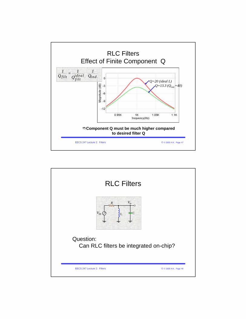
RLC Filters
•Bandpass filter:
Singularities: Complex conjugate poles + zeros and zero & infinity
o
so RC
2 2in oQ
o
o o
VV s s
1 LCRQ RC L
ω ω
ω
ω ω
=+ +
=
= =
oVR
CLinV
EECS 247 Lecture 2: Filters © © 2005 H.K. Page 46
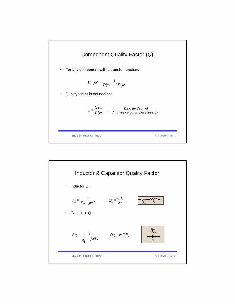
RLC Filters
•Design a bandpass filter with:•Center frequency of 1kHz•Q of 20
•Assume that the inductor has series R resulting in an inductor Q of 40•What is the effect of finite inductor Q on the overall Q?
oVR
CLinV
EECS 247 Lecture 2: Filters © © 2005 H.K. Page 47
RLC FiltersEffect of Finite Component Q
idealf i l t ind.f i l t
1 1 1Q QQ
= +
Q=20 (ideal L)Q=13.3 (Qind.=40)
eComponent Q must be much higher compared to desired filter Q
EECS 247 Lecture 2: Filters © © 2005 H.K. Page 48
RLC Filters
Question:Can RLC filters be integrated on-chip?
oVR
CLinV

EECS 247 Lecture 2: Filters © © 2005 H.K. Page 49
Monolithic InductorsFeasible Quality Factor & Value
vRef: “Radio Frequency Filters”, Lawrence Larson; Mead workshop presentation 1999
c Feasible monolithic inductor in CMOS tech. <10nH with Q <7
EECS 247 Lecture 2: Filters © © 2005 H.K. Page 50
Monolithic LC Filters
• Monolithic inductor in CMOS tech. – L<10nH with Q<7
• Max. capacitor size (based on realistic chip area)– C< 10pF
cLC filters in the monolithic form feasible: - Frequency >500MHz - Only low quality factor filters
Learn more in EE242

EECS 247 Lecture 2: Filters © © 2005 H.K. Page 51
Monolithic Filters
• Desirable to integrate filters with critical frequencies << 500MHz
• Per previous slide LC filters not a practical option in the integrated form for non-RF frequencies
• Good alternative:
cActive filters built without the need for inductors