Embed Size (px)
Citation preview
Filters and NoiseOptional Assessment of Practical Importance
Rubin H Landau
Sally Haerer, Producer-Director
Based on A Survey of Computational Physics by Landau, Páez, & Bordeianu
with Support from the National Science Foundation
Course: Computational Physics II
1 / 1
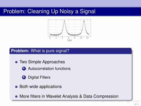
Problem: Cleaning Up Noisy a Signal
� � � � � � � � �
���� �
Problem: What is pure signal?
Two Simple Approaches1 Autocorrelation functions
2 Digital Filters
Both wide applications
More filters in Wavelet Analysis & Data Compression
2 / 1
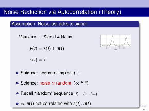
Noise Reduction via Autocorrelation (Theory)
Assumption: Noise just adds to signal
Measure = Signal + Noise
y(t) = s(t) + n(t)
s(t) = ?
� � � � � � � � �
���� �
Science: assume simplest (+)
Science: noise ' random (∞ o F)
Recall “random” sequence; ri ; ri+1
⇒ n(t) not correlated with s(t), n(t)3 / 1
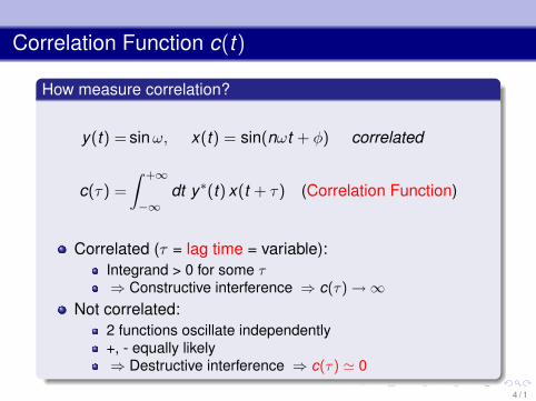
Correlation Function c(t)
How measure correlation?
y(t) = sinω, x(t) = sin(nωt + φ) correlated
c(τ) =
∫ +∞
−∞dt y∗(t) x(t + τ) (Correlation Function)
Correlated (τ = lag time = variable):Integrand > 0 for some τ⇒ Constructive interference ⇒ c(τ)→∞
Not correlated:2 functions oscillate independently+, - equally likely⇒ Destructive interference ⇒ c(τ) ' 0
4 / 1
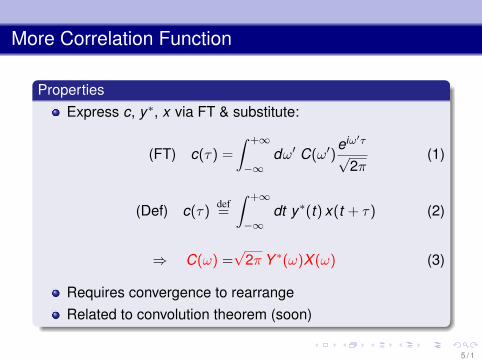
More Correlation Function
PropertiesExpress c, y∗, x via FT & substitute:
(FT) c(τ) =
∫ +∞
−∞dω′ C(ω′)
eiω′τ√
2π(1)
(Def) c(τ)def=
∫ +∞
−∞dt y∗(t) x(t + τ) (2)
⇒ C(ω) =√
2π Y ∗(ω)X (ω) (3)
Requires convergence to rearrangeRelated to convolution theorem (soon)
5 / 1
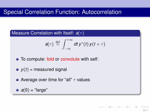
Special Correlation Function: Autocorrelation
Measure Correlation with Itself: a(τ)
a(τ)def=
∫ +∞
−∞dt y∗(t) y(t + τ)
To compute: fold or convolute with self:
y(t) = measured signal
Average over time for “all” τ values
a(0) = “large”
6 / 1
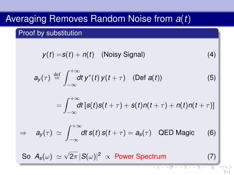
Averaging Removes Random Noise from a(t)Proof by substitution
y(t) =s(t) + n(t) (Noisy Signal) (4)
ay (τ)def=
∫ +∞
−∞dt y∗(t) y(t + τ) (Def a(t)) (5)
=
∫ +∞
−∞dt [s(t)s(t + τ) + s(t)n(t + τ) + n(t)n(t + τ)]
⇒ ay (τ) '∫ +∞
−∞dt s(t) s(t + τ) = as(τ) QED Magic (6)
So As(ω) '√
2π |S(ω)|2 ∝ Power Spectrum (7)
7 / 1
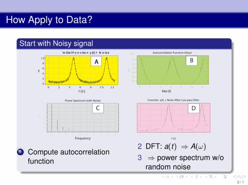
How Apply to Data?
Start with Noisy signal
0.0
0.5
1.0
1.5
2.0
2.5
3.0
3.5x10
3
0 5 10 15 20 25 30 35 40 45
Power Spectrum (with Noise)
Frequency
P
0
2
4
6
8
10
0 2 4 6 8 10 12
Function y(t) + Noise After Low pass Filter
t (s)
y
tau (s)
0.4
0.6
0.8
1.0
1.2
1.4
x102
0 2 4 6 8 10 12
Autocorrelation Function A(tau)
A
�
�
�
�
�
� �
� � � � � � � � �
�� ���� ��� � � � ��� � �� ����� �� � ���
���� �
�
AA B
C D
1 Compute autocorrelationfunction
2 DFT: a(t) ⇒ A(ω)
3 ⇒ power spectrum w/orandom noise
8 / 1
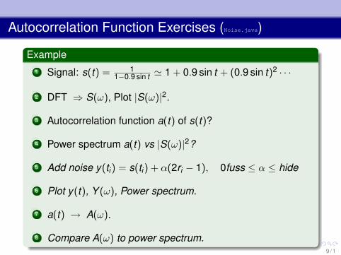
Autocorrelation Function Exercises (Noise.java)
Example1 Signal: s(t) = 1
1−0.9 sin t ' 1 + 0.9 sin t + (0.9 sin t)2 · · ·
2 DFT ⇒ S(ω), Plot |S(ω)|2.
3 Autocorrelation function a(t) of s(t)?
4 Power spectrum a(t) vs |S(ω)|2?
5 Add noise y(ti) = s(ti) + α(2ri − 1), 0fuss ≤ α ≤ hide
6 Plot y(t), Y (ω), Power spectrum.
7 a(t) → A(ω).
8 Compare A(ω) to power spectrum.9 / 1

Filtering with Transforms (Theory)
Action of Filter
g(t) =
∫ +∞
−∞dτ f (τ) h(t − τ) (8)
def= f (t) ∗ h(t) (analog filter) (9)
h(t) def= unit impulse
responseh(t) =
∫ +∞−∞ dτ δ(τ) h(t − τ)
Greens functionh(0) = max, h(< 0) = 0∗ = Convolution
10 / 1
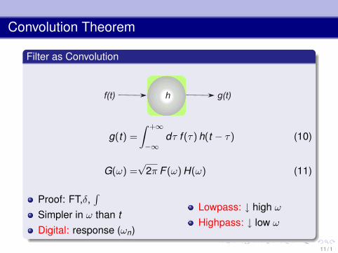
Convolution Theorem
Filter as Convolution
g(t) =
∫ +∞
−∞dτ f (τ) h(t − τ) (10)
G(ω) =√
2π F (ω) H(ω) (11)
Proof: FT,δ,∫
Simpler in ω than tDigital: response (ωn)
Lowpass: ↓ high ωHighpass: ↓ low ω
11 / 1
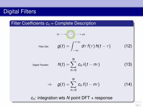
Digital Filters
Filter Coefficients cn = Complete Description
Filter Def: g(t) =
∫ +∞
−∞dτ f (τ) h(t − τ) (12)
Digital Transfer: h(t) =N∑
n=0
cn δ(t − nτ) (13)
⇒ g(t) =N∑
n=0
cn f (t − nτ) (14)
cn: integration wts N point DFT + response
12 / 1
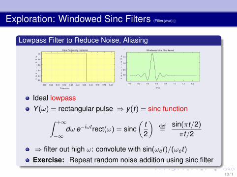
Exploration: Windowed Sinc Filters (Filter.java)�
Lowpass Filter to Reduce Noise, Aliasing
0.0
0.2
0.4
0.6
0.8
1.0
0.00 0.05 0.10 0.15 0.20 0.25 0.30 0.35 0.40 0.45 0.50
Ideal frequency response
Frequency
Amplitude
0.0
0.5
1.0
1.5
3
0.0 0.2 0.4 0.6 0.8 1.0 1.2 1.4
Windowed-sinc filter kernel
Time
Amplitude
Ideal lowpassY (ω) = rectangular pulse ⇒ y(t) = sinc function∫ +∞
−∞dω e−iωt rect(ω) = sinc
(t2
)def=
sin(πt/2)
πt/2
⇒ filter out high ω: convolute with sin(ωc t)/(ωc t)Exercise: Repeat random noise addition using sinc filter
13 / 1