Embed Size (px)
Citation preview

Filtered schemes for Hamilton-Jacobi equations
Tiago Salvadorjoint work with Adam Oberman
Department of Mathematics and Statistics
Numerical methods for Hamilton-Jacobi equations
in optimal control and related fields
RICAM, Linz, November 22, 2016

Hamilton-Jacobi equations Filtered Schemes Numerical schemes Explicit formulas Results Conclusions
Outline
1 Hamilton-Jacobi equations
2 Filtered Schemes
3 Numerical schemesSchemes for the Eikonal equationSchemes for Hamilton-Jacobi equations
4 Explicit formulasEikonal equationHJ equations
5 Results
6 Conclusions
Tiago Salvador Filtered schemes for Hamilton-Jacobi equations RICAM, 21-25 November 2016

Hamilton-Jacobi equations Filtered Schemes Numerical schemes Explicit formulas Results Conclusions
Contents
1 Hamilton-Jacobi equations
2 Filtered Schemes
3 Numerical schemesSchemes for the Eikonal equationSchemes for Hamilton-Jacobi equations
4 Explicit formulasEikonal equationHJ equations
5 Results
6 Conclusions
Tiago Salvador Filtered schemes for Hamilton-Jacobi equations RICAM, 21-25 November 2016

Hamilton-Jacobi equations Filtered Schemes Numerical schemes Explicit formulas Results Conclusions
Hamilton-Jacobi equations
Consider the Hamilton-Jacobi (HJ) equationH(x ,∇u) = f (x), x ∈ Ω \ Γ,u(x) = g(x), x ∈ Γ ⊂ Ω,
where
∇u is the gradient of the function u,
Ω is a bounded open set,
Γ is a subset of Ω,
H is a nonlinear Lipschitz continuous function.
Tiago Salvador Filtered schemes for Hamilton-Jacobi equations RICAM, 21-25 November 2016

Hamilton-Jacobi equations Filtered Schemes Numerical schemes Explicit formulas Results Conclusions
Eikonal equation
In particular, we will focus on the the Eikonal equation|∇u(x)| = f (x), for x outside Γ,
u(x) = g(x), for x on Γ,
where f > 0 and Γ is closed, bounded set.
Fact: Solutions are usually piecewise smooth and globally Lipschitz.
Tiago Salvador Filtered schemes for Hamilton-Jacobi equations RICAM, 21-25 November 2016

Hamilton-Jacobi equations Filtered Schemes Numerical schemes Explicit formulas Results Conclusions
Related work
Semi-Lagrangian schemes (Falconi, Ferretti ’02 and Cristiani,Falconi ’07)
Central schemes (Lin, Tadmor ’00)
ENO and WENO (Osher, Shu ’91)
Compact upwind second order scheme (Benamou, Luo, Zhao ’03)
Abgrall blended scheme (Abgrall ’09)
Tiago Salvador Filtered schemes for Hamilton-Jacobi equations RICAM, 21-25 November 2016

Hamilton-Jacobi equations Filtered Schemes Numerical schemes Explicit formulas Results Conclusions
Contents
1 Hamilton-Jacobi equations
2 Filtered Schemes
3 Numerical schemesSchemes for the Eikonal equationSchemes for Hamilton-Jacobi equations
4 Explicit formulasEikonal equationHJ equations
5 Results
6 Conclusions
Tiago Salvador Filtered schemes for Hamilton-Jacobi equations RICAM, 21-25 November 2016

Hamilton-Jacobi equations Filtered Schemes Numerical schemes Explicit formulas Results Conclusions
Motivation
In the one-dimensional case we are interested in solving |ux | = f (x). Themonotone (upwind) scheme is given by
∣∣uhx ∣∣M = max
−u(x + h)− u(x)
h,u(x)− u(x − h)
h, 0
= max
−D+u(x),D−u(x), 0
This scheme is also consistent and stable and so, by the Barles andSouganidis theory, it converges to the unique viscosity solution.
Fact: Monotone schemes are provably convergent but only first orderaccurate.
Tiago Salvador Filtered schemes for Hamilton-Jacobi equations RICAM, 21-25 November 2016

Hamilton-Jacobi equations Filtered Schemes Numerical schemes Explicit formulas Results Conclusions
We could consider the second order accurate centered scheme∣∣uhx ∣∣A =|u(x + h)− u(x − h)|
2h.
However this scheme is not monotone nor stable.
Fact: In general, higher order finite difference schemes for HJ equationsare neither monotone nor stable.
Up to a scaling in h, the difference of the schemes is the centered finitedifference approximation for |uxx |:∣∣∣∣∣uhx ∣∣A −
∣∣uhx ∣∣M ∣∣∣ = h
2
|u(x + h)− 2u(x) + u(x − h)|h2
=h
2uhxx(x).
We can then use this as a (local) criteria to decide whether or not to usethe accurate scheme.
Tiago Salvador Filtered schemes for Hamilton-Jacobi equations RICAM, 21-25 November 2016

Hamilton-Jacobi equations Filtered Schemes Numerical schemes Explicit formulas Results Conclusions
Filtered Schemes
The filtered scheme, |∇uh|F , then uses the following simple formula:
∣∣uhx ∣∣F =
∣∣uhx ∣∣A , if∣∣∣∣∣uhx ∣∣A −
∣∣uhx ∣∣M ∣∣∣ ≤ √h∣∣uhx ∣∣M , otherwise.
The filtered scheme, which is consistent provided both underlyingschemes are consistent, is usually not monotone. However it is almostmonotone, since∣∣uhx ∣∣F =
∣∣uhx ∣∣M +O(√h).
Tiago Salvador Filtered schemes for Hamilton-Jacobi equations RICAM, 21-25 November 2016

Hamilton-Jacobi equations Filtered Schemes Numerical schemes Explicit formulas Results Conclusions
Filtered Schemes
DefinitionS is a filter function if it is a bounded function that is equal to theidentity in a neighborhood of the origin and zero outside.
-2 -1 1 2
-1.0
-0.5
0.5
1.0
-3 -2 -1 1 2 3
-1.0
-0.5
0.5
1.0
DefinitionThe filtered scheme is given by F h[u] = F h
M [u] + ϵ(h)S(
F hA [u]−FM [u]
ϵ(h)
).
Tiago Salvador Filtered schemes for Hamilton-Jacobi equations RICAM, 21-25 November 2016
Hamilton-Jacobi equations Filtered Schemes Numerical schemes Explicit formulas Results Conclusions
Theorem (Froese, Oberman 2013)Let F h
M be a consistent, stable, monotone scheme. Assume S is acontinuous filter function and ϵ(h) → 0 as h → 0. For each h > 0, let uhbe a solution of F h[u] = 0, where the filtered scheme is given by
F h[u] = F hM [u] + ϵ(h)S
(F hA[u]− FM [u]
ϵ(h)
).
Then uh converges to the unique viscosity solution of the underlying PDE.
Why use filtered schemes?
Simplicity.
Provably convergent.
Achieve higher accuracy where the solution is smooth.
In practice, it avoids the use of a wide stencil in second orderequations (e.g. Monge-Ampere equation).
Tiago Salvador Filtered schemes for Hamilton-Jacobi equations RICAM, 21-25 November 2016

Hamilton-Jacobi equations Filtered Schemes Numerical schemes Explicit formulas Results Conclusions
Contents
1 Hamilton-Jacobi equations
2 Filtered Schemes
3 Numerical schemesSchemes for the Eikonal equationSchemes for Hamilton-Jacobi equations
4 Explicit formulasEikonal equationHJ equations
5 Results
6 Conclusions
Tiago Salvador Filtered schemes for Hamilton-Jacobi equations RICAM, 21-25 November 2016

Hamilton-Jacobi equations Filtered Schemes Numerical schemes Explicit formulas Results Conclusions
Schemes for the Eikonal equation
Schemes for the Eikonal equation
Monotone scheme
|uhx |M = max−D+u(x),D−u(x), 0
Accurate scheme (centred scheme)
|uhx |C ,2 =|u(x + h)− u(x − h)|
2h
High-order upwind scheme
|uhx |U,n = max
− d
dxP+,n[u](x),
d
dxP−,n[u](x), 0
ENO schemes
|uhx |E ,n = max
− d
dxE n, 12 [u](x),
d
dxE n,− 1
2 [u](x), 0
Tiago Salvador Filtered schemes for Hamilton-Jacobi equations RICAM, 21-25 November 2016

Hamilton-Jacobi equations Filtered Schemes Numerical schemes Explicit formulas Results Conclusions
Schemes for Hamilton-Jacobi equations
Schemes for Hamilton-Jacobi equations
Monotone scheme (Lax-Friedrichs)
HhLF [u](x) = Hh
LF (x ,D+u(x),D−u(x)) = H
(x ,
D+u(x) + D−u(x)
2
)−1
2σx (D
+u(x)−D−u(x))
Accurate scheme (centred scheme)
HhC ,2[u](x) = H
(x ,
u(x + h)− u(x − h)
2h
)High-order upwind scheme
HhU,n[u](x) = Hh
LF
(x ,
d
dxP+,n[u](x),
d
dxP−,n[u](x)
)ENO schemes
HhE ,n[u](x) = Hh
LF
(x ,
d
dxEn, 1
2 [u](x),d
dxEn,− 1
2 [u](x)
)
Tiago Salvador Filtered schemes for Hamilton-Jacobi equations RICAM, 21-25 November 2016

Hamilton-Jacobi equations Filtered Schemes Numerical schemes Explicit formulas Results Conclusions
Schemes for Hamilton-Jacobi equations
Schemes for Hamilton-Jacobi equations
Monotone scheme (Lax-Friedrichs)
HhLF [u](x) = Hh
LF (x ,D+u(x),D−u(x)) = H
(x ,
D+u(x) + D−u(x)
2
)−1
2σx (D
+u(x)−D−u(x))
Accurate scheme (centred scheme)
HhC ,2[u](x) = H
(x ,
u(x + h)− u(x − h)
2h
)
High-order upwind scheme
HhU,n[u](x) = Hh
LF
(x ,
d
dxP+,n[u](x),
d
dxP−,n[u](x)
)ENO schemes
HhE ,n[u](x) = Hh
LF
(x ,
d
dxEn, 1
2 [u](x),d
dxEn,− 1
2 [u](x)
)
Tiago Salvador Filtered schemes for Hamilton-Jacobi equations RICAM, 21-25 November 2016

Hamilton-Jacobi equations Filtered Schemes Numerical schemes Explicit formulas Results Conclusions
Schemes for Hamilton-Jacobi equations
Schemes for Hamilton-Jacobi equations
Monotone scheme (Lax-Friedrichs)
HhLF [u](x) = Hh
LF (x ,D+u(x),D−u(x)) = H
(x ,
D+u(x) + D−u(x)
2
)−1
2σx (D
+u(x)−D−u(x))
Accurate scheme (centred scheme)
HhC ,2[u](x) = H
(x ,
u(x + h)− u(x − h)
2h
)High-order upwind scheme
HhU,n[u](x) = Hh
LF
(x ,
d
dxP+,n[u](x),
d
dxP−,n[u](x)
)
ENO schemes
HhE ,n[u](x) = Hh
LF
(x ,
d
dxEn, 1
2 [u](x),d
dxEn,− 1
2 [u](x)
)
Tiago Salvador Filtered schemes for Hamilton-Jacobi equations RICAM, 21-25 November 2016

Hamilton-Jacobi equations Filtered Schemes Numerical schemes Explicit formulas Results Conclusions
Schemes for Hamilton-Jacobi equations
Schemes for Hamilton-Jacobi equations
Monotone scheme (Lax-Friedrichs)
HhLF [u](x) = Hh
LF (x ,D+u(x),D−u(x)) = H
(x ,
D+u(x) + D−u(x)
2
)−1
2σx (D
+u(x)−D−u(x))
Accurate scheme (centred scheme)
HhC ,2[u](x) = H
(x ,
u(x + h)− u(x − h)
2h
)High-order upwind scheme
HhU,n[u](x) = Hh
LF
(x ,
d
dxP+,n[u](x),
d
dxP−,n[u](x)
)ENO schemes
HhE ,n[u](x) = Hh
LF
(x ,
d
dxEn, 1
2 [u](x),d
dxEn,− 1
2 [u](x)
)
Tiago Salvador Filtered schemes for Hamilton-Jacobi equations RICAM, 21-25 November 2016

Hamilton-Jacobi equations Filtered Schemes Numerical schemes Explicit formulas Results Conclusions
Two-dimensional schemes
Two-dimensional schemes
Eikonal equation∣∣∇uh∣∣ = N
(∣∣uhx ∣∣ , ∣∣uhy ∣∣) where N(x , y) =√x2 + y2
Hamilton-Jacobi equations
HhLF [u](x) = Hh
LF (x , p+, p−, q+, q−)
= H
(x ,
p+ + p−
2,q+ + q−
2
)− σx
p+ − p−
2− σy
q+ − q−
2
where p± = D±x u(x) and q± = D±
y u(x).
Tiago Salvador Filtered schemes for Hamilton-Jacobi equations RICAM, 21-25 November 2016

Hamilton-Jacobi equations Filtered Schemes Numerical schemes Explicit formulas Results Conclusions
Contents
1 Hamilton-Jacobi equations
2 Filtered Schemes
3 Numerical schemesSchemes for the Eikonal equationSchemes for Hamilton-Jacobi equations
4 Explicit formulasEikonal equationHJ equations
5 Results
6 Conclusions
Tiago Salvador Filtered schemes for Hamilton-Jacobi equations RICAM, 21-25 November 2016

Hamilton-Jacobi equations Filtered Schemes Numerical schemes Explicit formulas Results Conclusions
Eikonal equation
Explicit formulas for Eikonal equation
Solving∣∣uhx ∣∣M = f for the reference variable, u(x), leads to
∣∣uhx ∣∣M = f ⇐⇒ max
−u(x + h)− u(x)
h,u(x)− u(x − h)
h, 0
= f (x)
⇐⇒ max u(x)− u(x + h), u(x)− u(x − h), 0 = hf (x)
⇐⇒ u(x) = minu(x + h), u(x − h)+ hf (x)
Similarly, for the second order upwind scheme we have∣∣uhx ∣∣U,2= f ⇐⇒ max3u(x)− 4u(x ± h) + u(x ± 2h), 0 = 2hf (x)
⇐⇒ u(x) =1
3min4u(x ± h)− u(x ± 2h)+ 2
3hf (x)
Tiago Salvador Filtered schemes for Hamilton-Jacobi equations RICAM, 21-25 November 2016

Hamilton-Jacobi equations Filtered Schemes Numerical schemes Explicit formulas Results Conclusions
Eikonal equation
Two-dimensional case
Solving∣∣∇uh∣∣ = f ⇐⇒
∣∣uhx ∣∣2 + ∣∣uhy ∣∣2 = f (x , y)2
for the reference variable u(x , y) requires solving nonlinear equation
maxz − a, 02 +maxz − b, 02 = c2
for the unknown z where a, b and c > 0 are constants. The uniquesolution is given by
z =
mina, b+ c , |a− b| ≥ c ,a+b+
√2c2−(a−b)2
2 , |a− b| < c .
Tiago Salvador Filtered schemes for Hamilton-Jacobi equations RICAM, 21-25 November 2016

Hamilton-Jacobi equations Filtered Schemes Numerical schemes Explicit formulas Results Conclusions
HJ equations
Explicit formulas for the HJ equations
Recall that
D+u(x) =u(x + h)− u(x)
h, D−u(x) =
u(x)− u(x − h)
h.
Solving HhLF [u] = f for the reference variable, u(x), leads to
H
(x ,
D+u(x) + D−u(x)
2
)−
1
2σx(D+u(x)− D−u(x)
)= f (x)
⇐⇒ H
(x ,
u(x + h)− u(x − h)
2h
)−
1
2σx
u(x + h)− 2u(x) + u(x − h)
h= f (x)
⇐⇒ u(x) =1
σx
[f (x)− H
(x ,
u(x + h)− u(x − h)
2h
)+ σx
u(x + h) + u(x − h)
2h
].
Tiago Salvador Filtered schemes for Hamilton-Jacobi equations RICAM, 21-25 November 2016
Hamilton-Jacobi equations Filtered Schemes Numerical schemes Explicit formulas Results Conclusions
HJ equations
Explicit formulas for the HJ equations
Consider now the second order upwind scheme, HhU,2[u] = f , rewritten as
H
(x ,
ddxP+,2[u](x) + d
dxP−,2[u](x)
2
)−
1
2σx
(d
dxP+,2[u](x)−
d
dxP−,2[u](x)
)= f (x).
where
d
dxP+,2[u](x) =
−3u(x) + 4u(x + h)− u(x + 2h)
2h,
d
dxP−,2[u](x) =
3u(x)− 4u(x − h) + u(x − 2h)
2h.
Thus, solving for the reference variable, u(x), leads to
u(x) =2
3σx
[f (x)− H
(x ,
−u(x + 2h) + 4u(x + h)− 4u(x − h) + u(x − 2h)
4h
)+σx
−u(x + 2h) + 4u(x + h) + 4u(x − h)− u(x − 2h)
4h
].
Tiago Salvador Filtered schemes for Hamilton-Jacobi equations RICAM, 21-25 November 2016

Hamilton-Jacobi equations Filtered Schemes Numerical schemes Explicit formulas Results Conclusions
Contents
1 Hamilton-Jacobi equations
2 Filtered Schemes
3 Numerical schemesSchemes for the Eikonal equationSchemes for Hamilton-Jacobi equations
4 Explicit formulasEikonal equationHJ equations
5 Results
6 Conclusions
Tiago Salvador Filtered schemes for Hamilton-Jacobi equations RICAM, 21-25 November 2016
Hamilton-Jacobi equations Filtered Schemes Numerical schemes Explicit formulas Results Conclusions
One-dimensional examples
The 1st example is given by
|ux | = 1 + cos(x), u(x) = 3− |x + sin(x)|
−2 −1.5 −1 −0.5 0 0.5 1 1.5 20
0.5
1
1.5
2
2.5
3
Figure: Profile of the solution.
Tiago Salvador Filtered schemes for Hamilton-Jacobi equations RICAM, 21-25 November 2016
Hamilton-Jacobi equations Filtered Schemes Numerical schemes Explicit formulas Results Conclusions
−0.4 −0.3 −0.2 −0.1 0 0.1 0.2 0.3 0.42.5
2.55
2.6
2.65
2.7
2.75
2.8
2.85
2.9
2.95
3
Monotone
2ndupwind
Exact
Figure: Exact solution and solutions obtained with the monotone scheme andthe 2nd order upwind filtered scheme with 50 grid points.
Tiago Salvador Filtered schemes for Hamilton-Jacobi equations RICAM, 21-25 November 2016
Hamilton-Jacobi equations Filtered Schemes Numerical schemes Explicit formulas Results Conclusions
−2 −1.5 −1 −0.5 0 0.5 1 1.5 20
0.1
0.2
0.3
0.4
0.5
0.6
0.7
0.8
0.9
1
−2 −1.5 −1 −0.5 0 0.5 1 1.5 20
0.1
0.2
0.3
0.4
0.5
0.6
0.7
0.8
0.9
1
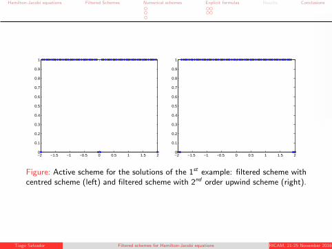
Figure: Active scheme for the solutions of the 1st example: filtered scheme withcentred scheme (left) and filtered scheme with 2nd order upwind scheme (right).
Tiago Salvador Filtered schemes for Hamilton-Jacobi equations RICAM, 21-25 November 2016
Hamilton-Jacobi equations Filtered Schemes Numerical schemes Explicit formulas Results Conclusions
101
102
103
104
10−12
10−10
10−8
10−6
10−4
10−2
100
MonotoneFiltered (2nd)Filtered (2ndUpwind)Filtered (3rdUpwind)Filtered (4thUpwind)Filtered (2ndENO)Filtered (3rdENO)Filtered (4thENO)
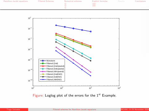
Figure: Loglog plot of the errors for the 1st Example.
Tiago Salvador Filtered schemes for Hamilton-Jacobi equations RICAM, 21-25 November 2016
Hamilton-Jacobi equations Filtered Schemes Numerical schemes Explicit formulas Results Conclusions
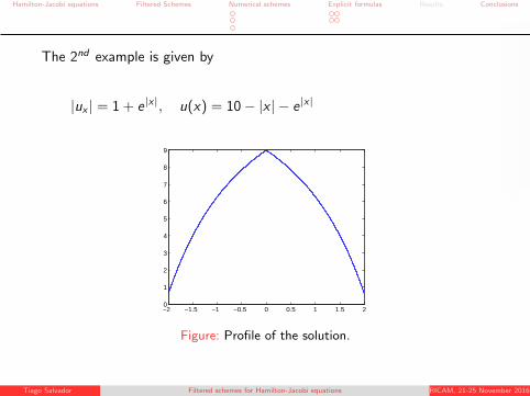
The 2nd example is given by
|ux | = 1 + e|x|, u(x) = 10− |x | − e|x|
−2 −1.5 −1 −0.5 0 0.5 1 1.5 20
1
2
3
4
5
6
7
8
9
Figure: Profile of the solution.
Tiago Salvador Filtered schemes for Hamilton-Jacobi equations RICAM, 21-25 November 2016
Hamilton-Jacobi equations Filtered Schemes Numerical schemes Explicit formulas Results Conclusions
101
102
103
104
10−12
10−10
10−8
10−6
10−4
10−2
100
MonotoneFiltered (2nd)Filtered (2ndUpwind)Filtered (3rdUpwind)Filtered (4thUpwind)Filtered (2ndENO)Filtered (3rdENO)Filtered (4thENO)
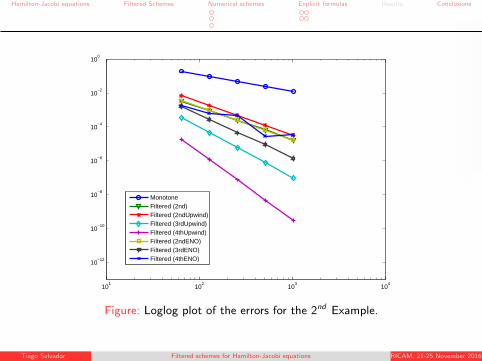
Figure: Loglog plot of the errors for the 2nd Example.
Tiago Salvador Filtered schemes for Hamilton-Jacobi equations RICAM, 21-25 November 2016

Hamilton-Jacobi equations Filtered Schemes Numerical schemes Explicit formulas Results Conclusions
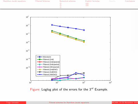
The 3rd example is given by
|ux | = 3x2 + a, u(x) =
x3 + ax , x ∈ [0, x0],
1 + a− ax − x3, x ∈ [x0, 1],
with a =1−2x3
0
2x0−1 , x0 =3√2+24 3√2
.
0 0.2 0.4 0.6 0.8 10
0.2
0.4
0.6
0.8
1
1.2
1.4
Figure: Profile of the solution.
Tiago Salvador Filtered schemes for Hamilton-Jacobi equations RICAM, 21-25 November 2016
Hamilton-Jacobi equations Filtered Schemes Numerical schemes Explicit formulas Results Conclusions
101
102
103
104
10−12
10−10
10−8
10−6
10−4
10−2
100
MonotoneFiltered (2nd)Filtered (2ndUpwind)Filtered (3rdUpwind)Filtered (4thUpwind)Filtered (2ndENO)Filtered (3rdENO)Filtered (4thENO)
Figure: Loglog plot of the errors for the 3rd Example.
Tiago Salvador Filtered schemes for Hamilton-Jacobi equations RICAM, 21-25 November 2016

Hamilton-Jacobi equations Filtered Schemes Numerical schemes Explicit formulas Results Conclusions
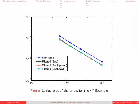
The 4th example is given by
|ux |2 = ex , u(x) =
2e
x2 + 16, x x ∈ [−2, 0],
−2ex2 + 20, x ∈ [0, 2].
−2 −1.5 −1 −0.5 0 0.5 1 1.5 214.5
15
15.5
16
16.5
17
17.5
18
Figure: Profile of the solution.
Tiago Salvador Filtered schemes for Hamilton-Jacobi equations RICAM, 21-25 November 2016
Hamilton-Jacobi equations Filtered Schemes Numerical schemes Explicit formulas Results Conclusions
101
102
103
10−3
10−2
10−1
100
MonotoneFiltered (2nd)Filtered (2ndUpwind)Filtered (2ndENO)
Figure: Loglog plot of the errors for the 4th Example.
Tiago Salvador Filtered schemes for Hamilton-Jacobi equations RICAM, 21-25 November 2016
Hamilton-Jacobi equations Filtered Schemes Numerical schemes Explicit formulas Results Conclusions
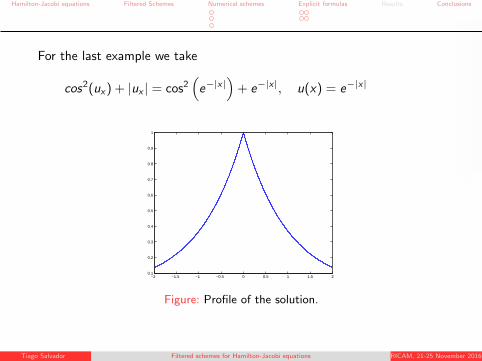
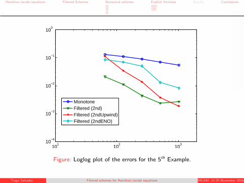
For the last example we take
cos2(ux) + |ux | = cos2(e−|x|
)+ e−|x|, u(x) = e−|x|
−2 −1.5 −1 −0.5 0 0.5 1 1.5 20.1
0.2
0.3
0.4
0.5
0.6
0.7
0.8
0.9
1
Figure: Profile of the solution.
Tiago Salvador Filtered schemes for Hamilton-Jacobi equations RICAM, 21-25 November 2016
Hamilton-Jacobi equations Filtered Schemes Numerical schemes Explicit formulas Results Conclusions
101
102
103
10−4
10−3
10−2
10−1
100
MonotoneFiltered (2nd)Filtered (2ndUpwind)Filtered (2ndENO)
Figure: Loglog plot of the errors for the 5th Example.
Tiago Salvador Filtered schemes for Hamilton-Jacobi equations RICAM, 21-25 November 2016
Hamilton-Jacobi equations Filtered Schemes Numerical schemes Explicit formulas Results Conclusions
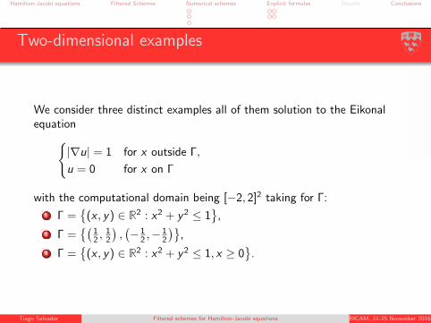
Two-dimensional examples
We consider three distinct examples all of them solution to the Eikonalequation
|∇u| = 1 for x outside Γ,
u = 0 for x on Γ
with the computational domain being [−2, 2]2 taking for Γ:
1 Γ =(x , y) ∈ R2 : x2 + y2 ≤ 1
,
2 Γ =(
12 ,
12
),(− 1
2 ,−12
),
3 Γ =(x , y) ∈ R2 : x2 + y2 ≤ 1, x ≥ 0
.
Tiago Salvador Filtered schemes for Hamilton-Jacobi equations RICAM, 21-25 November 2016
Hamilton-Jacobi equations Filtered Schemes Numerical schemes Explicit formulas Results Conclusions
−2−1
01
2
−2
−1
0
1
20
0.5
1
1.5
2
−2−1
01
2 −2
0
20
0.5
1
1.5
2
2.5
3
−2
−1
0
1
2
−2
−1
0
1
20
0.5
1
1.5
2
2.5
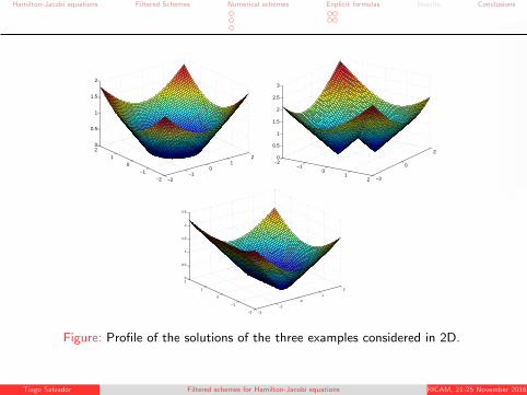
Figure: Profile of the solutions of the three examples considered in 2D.
Tiago Salvador Filtered schemes for Hamilton-Jacobi equations RICAM, 21-25 November 2016
Hamilton-Jacobi equations Filtered Schemes Numerical schemes Explicit formulas Results Conclusions
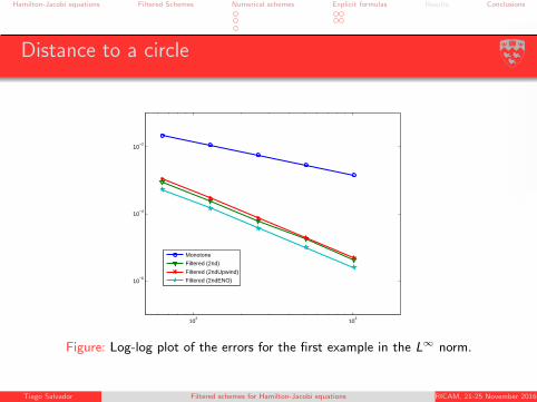
Distance to a circle
102
103
10−6
10−4
10−2
Monotone
Filtered (2nd)
Filtered (2ndUpwind)
Filtered (2ndENO)
Figure: Log-log plot of the errors for the first example in the L∞ norm.
Tiago Salvador Filtered schemes for Hamilton-Jacobi equations RICAM, 21-25 November 2016
Hamilton-Jacobi equations Filtered Schemes Numerical schemes Explicit formulas Results Conclusions
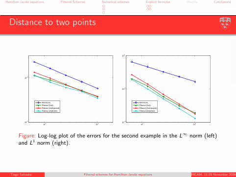
Distance to two points
102
103
10−4
10−2
Monotone
Filtered (2nd)
Filtered (2ndUpwind)
Filtered (2ndENO)
102
103
10−4
10−2
100
Monotone
Filtered (2nd)
Filtered (2ndUpwind)
Filtered (2ndENO)
Figure: Log-log plot of the errors for the second example in the L∞ norm (left)and L1 norm (right).
Tiago Salvador Filtered schemes for Hamilton-Jacobi equations RICAM, 21-25 November 2016
Hamilton-Jacobi equations Filtered Schemes Numerical schemes Explicit formulas Results Conclusions
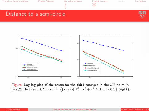
Distance to a semi-circle
102
103
10−4
10−2
Monotone
Filtered (2nd)
Filtered (2ndUpwind)
Filtered (2ndENO)
102
103
10−6
10−4
10−2
Monotone
Filtered (2nd)
Filtered (2ndUpwind)
Filtered (2ndENO)
Figure: Log-log plot of the errors for the third example in the L∞ norm in[−2, 2] (left) and L∞ norm in
(x , y) ∈ R2 : x2 + y 2 ≥ 1, x > 0.1
(right).
Tiago Salvador Filtered schemes for Hamilton-Jacobi equations RICAM, 21-25 November 2016

Hamilton-Jacobi equations Filtered Schemes Numerical schemes Explicit formulas Results Conclusions
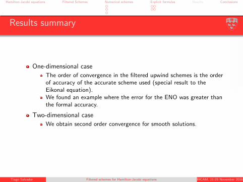
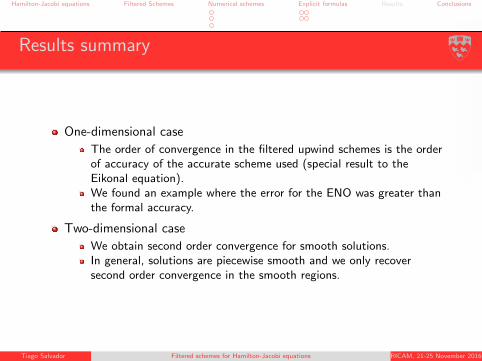
Results summary
One-dimensional case
The order of convergence in the filtered upwind schemes is the orderof accuracy of the accurate scheme used (special result to theEikonal equation).We found an example where the error for the ENO was greater thanthe formal accuracy.
Two-dimensional case
We obtain second order convergence for smooth solutions.In general, solutions are piecewise smooth and we only recoversecond order convergence in the smooth regions.
Tiago Salvador Filtered schemes for Hamilton-Jacobi equations RICAM, 21-25 November 2016

Hamilton-Jacobi equations Filtered Schemes Numerical schemes Explicit formulas Results Conclusions
Results summary
One-dimensional case
The order of convergence in the filtered upwind schemes is the orderof accuracy of the accurate scheme used (special result to theEikonal equation).
We found an example where the error for the ENO was greater thanthe formal accuracy.
Two-dimensional case
We obtain second order convergence for smooth solutions.In general, solutions are piecewise smooth and we only recoversecond order convergence in the smooth regions.
Tiago Salvador Filtered schemes for Hamilton-Jacobi equations RICAM, 21-25 November 2016

Hamilton-Jacobi equations Filtered Schemes Numerical schemes Explicit formulas Results Conclusions
Results summary
One-dimensional case
The order of convergence in the filtered upwind schemes is the orderof accuracy of the accurate scheme used (special result to theEikonal equation).We found an example where the error for the ENO was greater thanthe formal accuracy.
Two-dimensional case
We obtain second order convergence for smooth solutions.In general, solutions are piecewise smooth and we only recoversecond order convergence in the smooth regions.
Tiago Salvador Filtered schemes for Hamilton-Jacobi equations RICAM, 21-25 November 2016

Hamilton-Jacobi equations Filtered Schemes Numerical schemes Explicit formulas Results Conclusions
Results summary
One-dimensional case
The order of convergence in the filtered upwind schemes is the orderof accuracy of the accurate scheme used (special result to theEikonal equation).We found an example where the error for the ENO was greater thanthe formal accuracy.
Two-dimensional case
We obtain second order convergence for smooth solutions.In general, solutions are piecewise smooth and we only recoversecond order convergence in the smooth regions.
Tiago Salvador Filtered schemes for Hamilton-Jacobi equations RICAM, 21-25 November 2016
Hamilton-Jacobi equations Filtered Schemes Numerical schemes Explicit formulas Results Conclusions
Results summary
One-dimensional case
The order of convergence in the filtered upwind schemes is the orderof accuracy of the accurate scheme used (special result to theEikonal equation).We found an example where the error for the ENO was greater thanthe formal accuracy.
Two-dimensional case
We obtain second order convergence for smooth solutions.
In general, solutions are piecewise smooth and we only recoversecond order convergence in the smooth regions.
Tiago Salvador Filtered schemes for Hamilton-Jacobi equations RICAM, 21-25 November 2016
Hamilton-Jacobi equations Filtered Schemes Numerical schemes Explicit formulas Results Conclusions
Results summary
One-dimensional case
The order of convergence in the filtered upwind schemes is the orderof accuracy of the accurate scheme used (special result to theEikonal equation).We found an example where the error for the ENO was greater thanthe formal accuracy.
Two-dimensional case
We obtain second order convergence for smooth solutions.In general, solutions are piecewise smooth and we only recoversecond order convergence in the smooth regions.
Tiago Salvador Filtered schemes for Hamilton-Jacobi equations RICAM, 21-25 November 2016

Hamilton-Jacobi equations Filtered Schemes Numerical schemes Explicit formulas Results Conclusions
Contents
1 Hamilton-Jacobi equations
2 Filtered Schemes
3 Numerical schemesSchemes for the Eikonal equationSchemes for Hamilton-Jacobi equations
4 Explicit formulasEikonal equationHJ equations
5 Results
6 Conclusions
Tiago Salvador Filtered schemes for Hamilton-Jacobi equations RICAM, 21-25 November 2016

Hamilton-Jacobi equations Filtered Schemes Numerical schemes Explicit formulas Results Conclusions
Conclusions
Filtered schemes:
are provably convergent;
are simple and easy to implement;
allow for a wide choice of accurate discretizations;
achieve higher accuracy where the solution is smooth;
in practice, it avoids the use of a wide stencil in second orderequations (e.g. Monge-Ampere equation).
Tiago Salvador Filtered schemes for Hamilton-Jacobi equations RICAM, 21-25 November 2016

Hamilton-Jacobi equations Filtered Schemes Numerical schemes Explicit formulas Results Conclusions
References
Guy Barles and Panagiotis E. Souganidis, Convergence ofapproximation schemes for fully nonlinear second order equations,Asymptotic Anal. 4 (1991).
Brittany D. Froese and Adam M. Oberman, Convergent filteredschemes for the Monge-Ampere partial differential equation, SIAM J.Numer. Anal. 51 (2013).
Stanley Osher and Chi-Wang Shu, High-order essentiallynonoscillatory schemes for Hamilton-Jacobi equations, SIAM J.Numer. Anal. 28 (1991).
Hongkai Zhao, A fast sweeping method for eikonal equations, Math.Comp. 74 (2005).
Adam M. Oberman and Tiago Salvador, Filtered schemes forHamilton-Jacobi equations: a simple construction of convergentaccurate difference schemes, JCP 284 (2015).
Tiago Salvador Filtered schemes for Hamilton-Jacobi equations RICAM, 21-25 November 2016