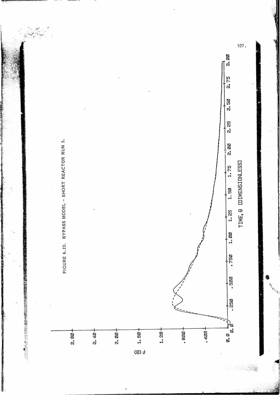
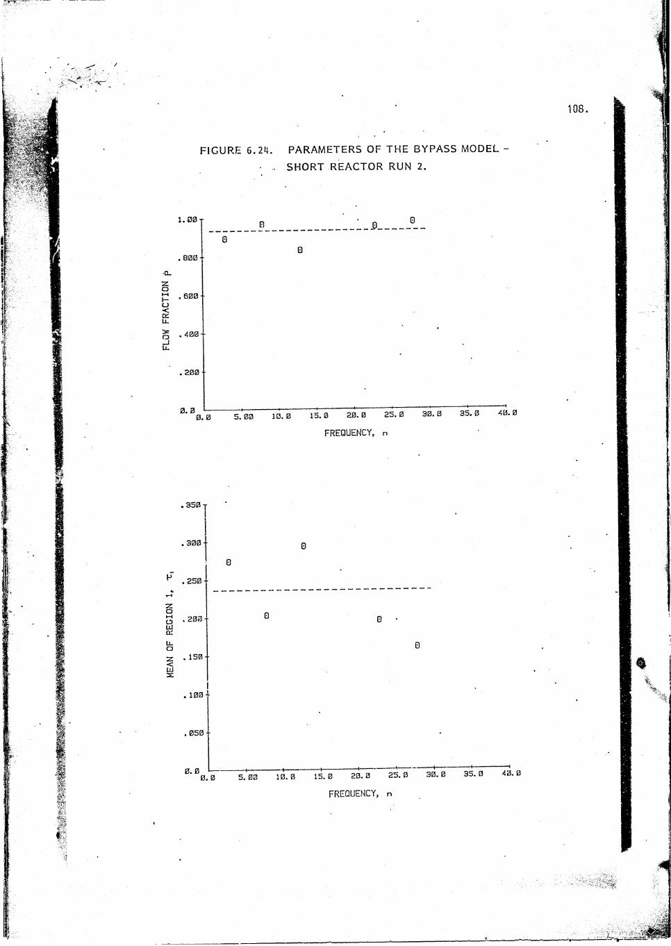
FIGURE 6.24. PARAMETERS OF THE BYPASS MODEL

. SHORT REACTOR RUN 2.

FREQUENCY, n

FREQUENCY, n

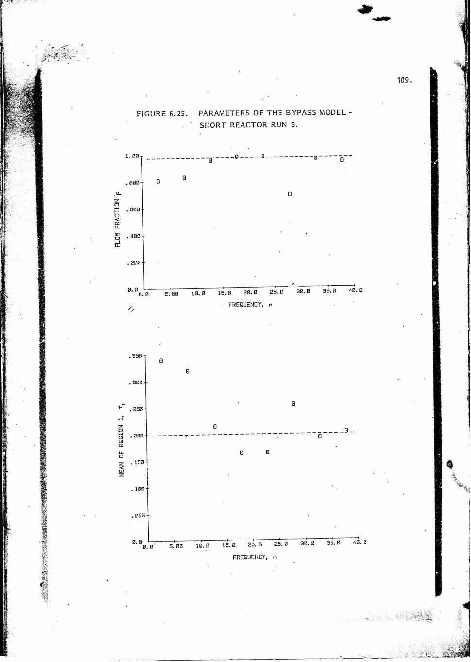
FIGURE 6.25. PARAMETERS OF THE BYPASS MODEL

" SHORT REACTOR RUN 5.

FREQUENCY, n

FREQUENCY, n

7. CONCLUSIONS

Digital radiation counting tecbniqes are found to be suitable ior measuring very short residence time distributions (down to a mean residence time of 0,4 sec). By using high count rates and care-fully selected counting periods, the statistical radiation error

and instrument error can be kept small.

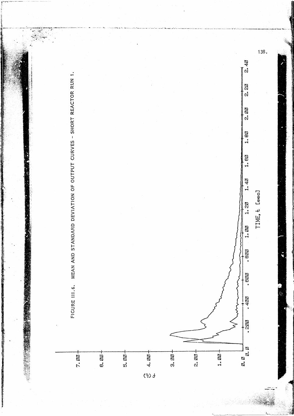
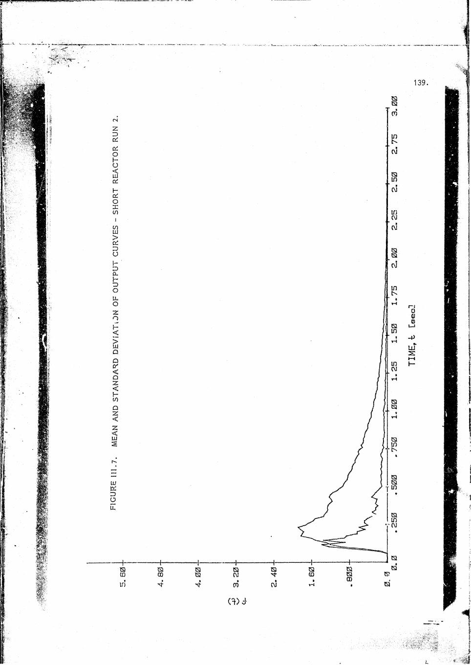
Flow patterns in the vessels are shown to fluctuate with time, and experiments have to be repeated and averaged to obtain a represen­

tative curve.

The flow patterns are independent of flowrate over the range in- vestigated (turbulent conditions). This is in agreement with thefindings of Clegg (11) for a cylindrical vessel also exhibiting

internal recycle.

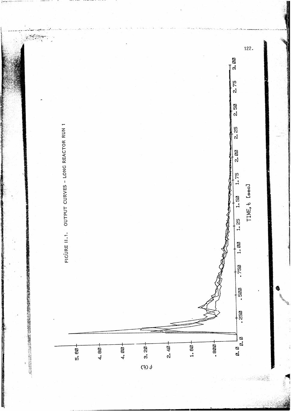
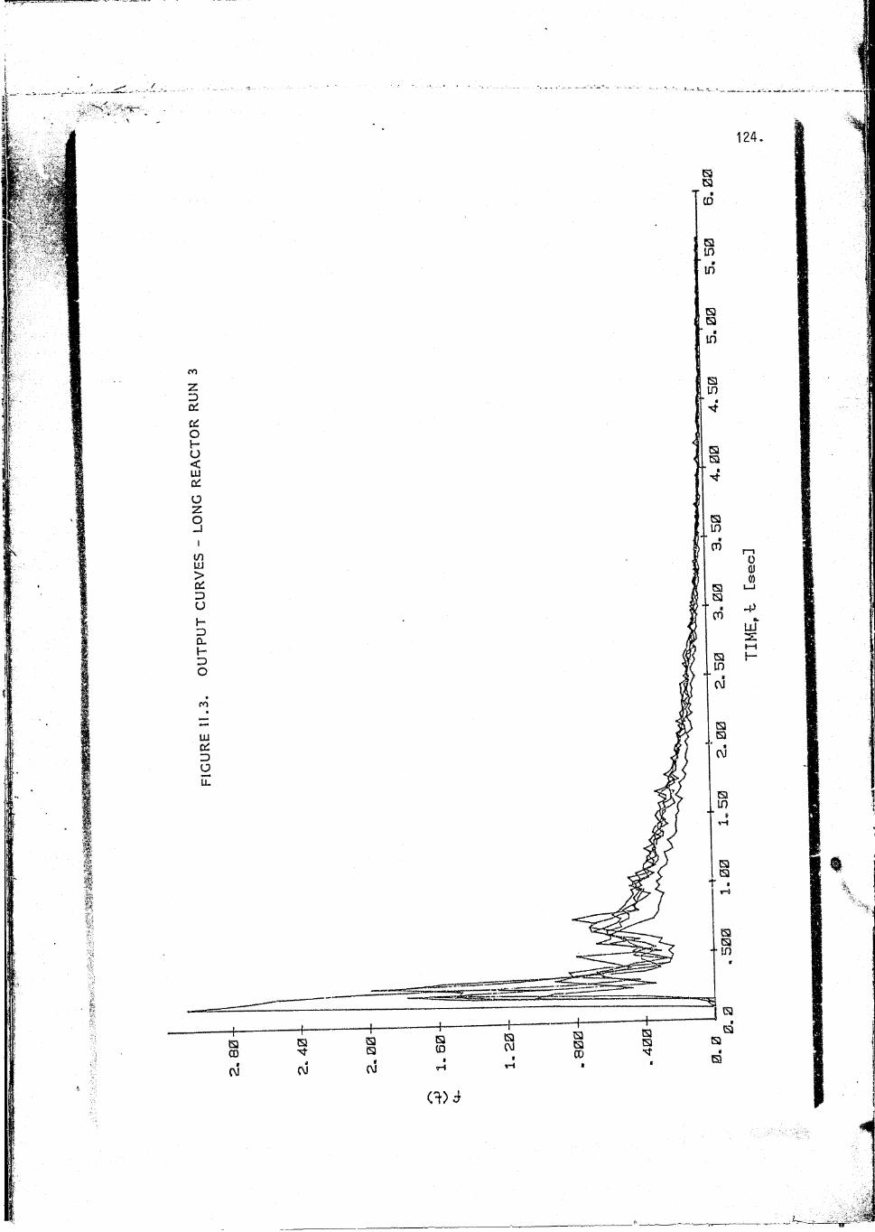
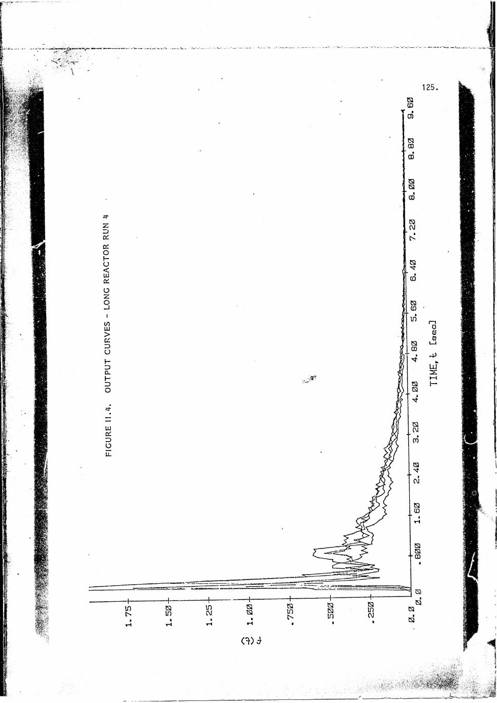
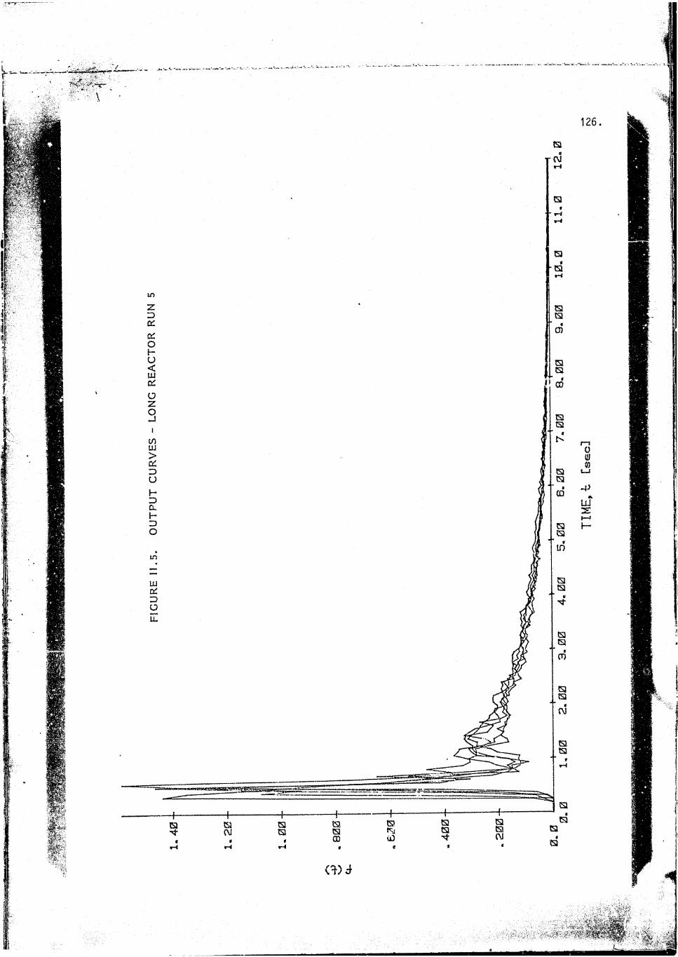
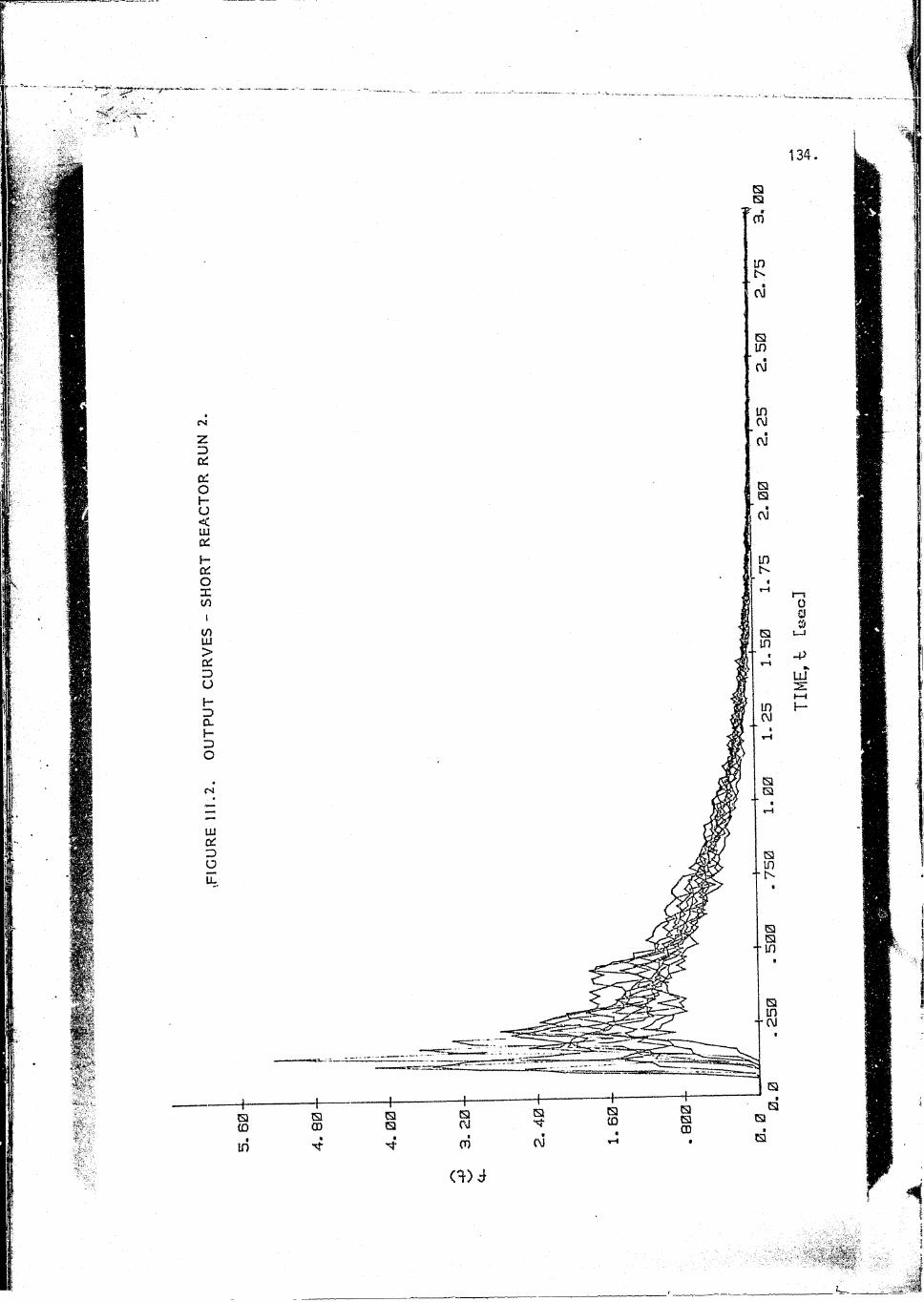
In comparing the RTD curves of the two lengths of reactor, it can be seen that the effect of reducing the vessel length is to in-crcase the "mixedness" in the vessel. The short reactor RTD curve does not differ significantly from that of a CSTR, while the long reactor curve shows the peaks characteristic of recycling. Forboth vessels the tails of the curves decay exponentially. The large first peak in the long reactor RTD curve would result in lower conversions per unit volume for this reactor shape than for the short reactor for most reaction schemes. If one were to increase the reactor length further, the first peak would become more emphasised but its position would shift towards 8=1 and the recycle fraction would decrease, approaching plug flow for verylarge 1/d ratio. It thus appears that the 1/d ratio given by thelong reactor is less attractive than either a small 1/d (wellmixed) or a much larger 1/d (plug flow). One cannot however ex- trapolate the results of only two reactor lengths to much larger 1/d ratios, and further research would be required. There arenaturally other factors which must be considered in comparing reactor types, e.g. the effect of recirculation in heating up the reactants in the case of autothermal reactions.

Flow patterns in the longer vessel are well modelled by a simplerecycle model. The forward flow region shows a small amount ofbackmixing ’ and is adequately represented by a gamma distribution (tanks-in-series model) or an axial dispersion model. The recycle region is well mixed and can be represented by a CSTR. The mean residence time in the forward region is about 0,2 of the overall mean residence time and this region comprises about 70% of thetotal reactor volume. The recycle fraction is approximately 0,7.

Less information could be extracted from the smoother RTD curves of the short vessel. This reactor can adequately be represented by ' a gamma distribution with little backmixing, followed by a CSTR, with a small bypass (4%) around the CSTR. The first region makes up about 20% of the vessel volume. For approximate engi- neering calculations however, the short vessel can be assumed to

be a CSTR.

Scale-up of the results to a full sized reactor is simplified by the fact that the flow patterns are independent of flowrate.Dynamic similarity is therefore not required, so long as the Reynolds number is high enough so that the flow is turbulent. The only two scaling criteria as far as flow patterns are concerned are therefore geometric similarity and allowances for density changes in a reacting system. Allowance for density changes is usually made by assuming that all gas expansion takes place imme­diately upon entering the reactor. The inlet nozzles are there­fore scaled by an additional factor equal to the square root of the ratio of expansion of the gases in the reactor (23,24). Expansion due to chemical reaction (change in number of moles) as well as _emperature change is treated in this way.

The type of reactor investigated in this work can be used in many applications where intense mixing of gases- is required. Its greatest application is where internal recirculation is required e.g. for autothermal reactions such as combustion systems. It can also be used for gas-particle reactions where a high level of tur­

bulence is required e.g. pulverised coal gasification. Besidestheir application to represent flow inside vessels, the recycle flow models developed here can be applied to numerous other pro­cesses based on recirculation, e.g. catalytic cracking, particle coating, granulation and crystallisation (15).

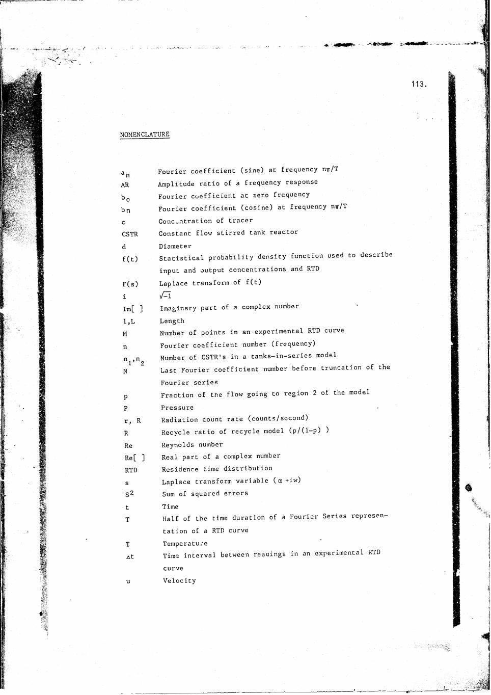
NOMENCLATURE

a Fourier coefficient (sine) at frequency mr/TAR Amplitude ratio of a frequency responseb0 Fourier coefficient at zero frequencyb n Fourier coefficient (cosine) at frequency mr/Tc Concentration of tracerCSTR Constant flow stirred tank reactord Diameterf(t) Statistical probability density function used to desc

input and output concentrations and RTD F(s) Laplace transform of f(t)ilro[ ] Imaginary part of a complex number

1,L LengthM Number of points in an experimental RTD curven Fourier coefficient number (frequency)n ,n Number of CSTR's in a tanks-in-series modelN Last Fourier coefficient number before truncation of

Fourier seriesp Fraction of the flow going to region 2 of the modelP Pressurer, R Radiation count rate (counts/second)R Recycle ratio of recycle model (p/(l-p) )Re Reynolds numberRe[ ] Real part of a complex number RTD Residence time distributions Laplace transform variable (a +iw)S2 Sum of squared errorst TimeT Half of the time duration of a Fourier Series repres

tation of a RTD curve T TemperatureAt Time interval between readings in an experimental RT

curve

114.

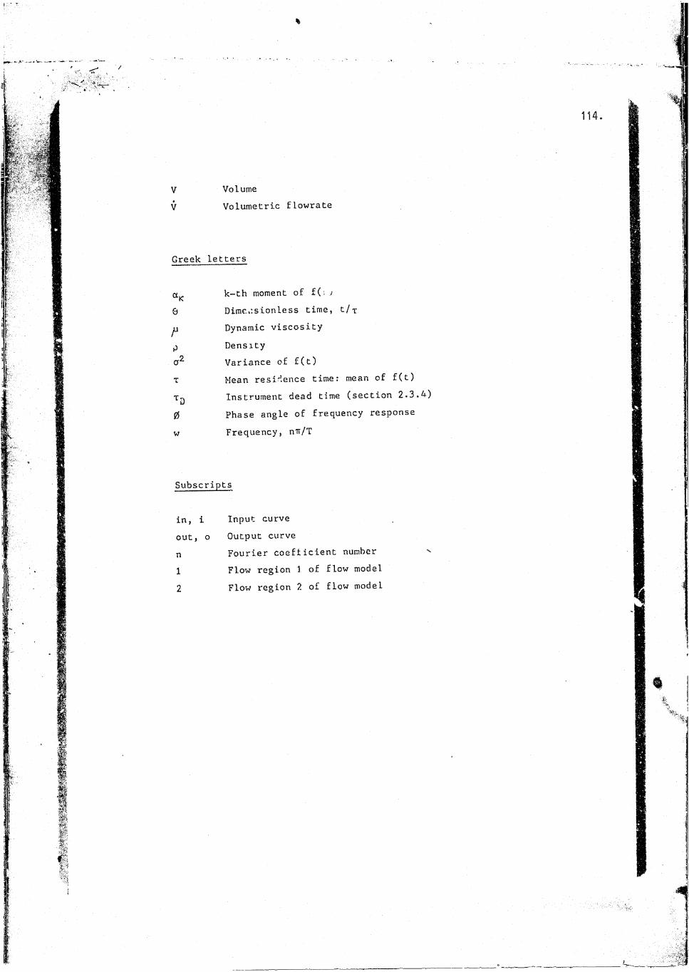
Vv

VolumeVolumetric flowrate

Greek letters

0w

k-th moment of f(: .>Dime.tsionless time, t/x Dynamic viscosity DensityVariance of f(t)Mean residence time: mean of f(t) Instrument dead time (section 2.3.4) Phase angle of frequency response Frequency, nu/T

Subscripts

in, i out, o n 1 2

Input curve Output curveFourier coefficient number Flow region 1 of flow model Flow region 2 of flow model

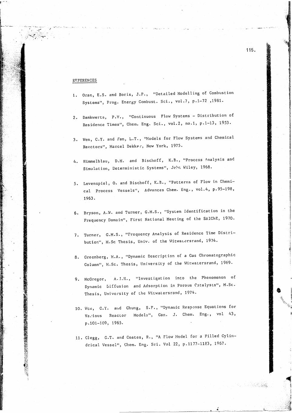
REFERENCES

1. Oran, E.S. and Boris, J.P., "Detailed Modelling of CombustionSystems", Prog. Energy Combust. Sci., vol.7, p.1-72 ,1981.

2. Dankwerts, P .V ., "Continuous Flow Systems - Distribution of Residence Times", Chem. Eng. Sci., vol.2, no.l, p.1-13, 1953.

3. Wen, C.Y. and Fan, L.T., "Models for Flow Systems and Chemical Reactors", Marcel Dekker, New York, 1975.

4. Himmelblau, D.M. and Bischoff, K.B., "Process Analysis and Simulation, Deterministic Systems", John Wiley, 1968.

5. Levenspiel, 0. and Bischoff, K.B., "Patterns of Flow in Chemi-cal Process Vessels", Advances Chem, Eng. , vol.4, p.95-198,

1963.

6. Bryson, A.W. and Turner, G.M.S., "System Identification in the Frequency Domain", First National Meeting of the SAIChE, 1970.

7. Turner, G.M.S., "Frequency Analysis of Residence Time Distri­bution", M.Sc Thesis, Univ. of the Witwacersrand, 1974.

8. Greenberg, M.A., "Dynamic Description of a Gas Chromatographic Column", M.Sc. Thesis, University of the Witwatersrand, 1969.

9. McGregor, "Investigation into the Phenomenon ofDynamic Diffusion and Adsorption in Porous Catalysts", M.Sc. Thesis, University of the Witwatersrand, 1974.

10. Wen, C.Y. and Chung, S.F., "Dynamic Response Equations for Various Reactor Models", Can. J. Chem. Eng., vol 43,

p.101-109, 1965.

11. Clegg, G.T. and Coates, R., "A Flow Model for a Filled Cylin-drical Vessel", Chem. Eng, Sci. Vol 22, p.1177-1183, 1967.

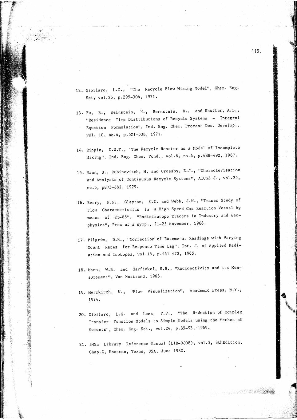
12. Gibilaro, L.G., "The Recycle Flow Mixing Model", Chem. Eng.Sci, vol.26, p.299—304, 1971.

13. Fu, B., Weinstein, H., Bernstein, B., and Shaffer, A.B., "Residence Time Distributions of Recycle Systems - Integral Equation Formulation", Ind. Eng. Chem. Process Des. Develop., vol. 10, no.4, p.501-508, 1971.

14. Rippin, D.W.T., 'The Recycle Reactor as a Model of Incomplete Mixing", Ind. Eng. Chem. Fund., vol.6, no.4, p.488-492, 1967.

15. Mann, U., Rubinovitch, M. and Crossby, E,. J., "Characterisation and Analysis of Continuous Recycle Systems", AIChE J., vol.25,

no.5, p873-882, 1979.

16. Berry, P.P., Clayton, C.G. and Webb, J.W., "Tracer Study of Flow Characteristics in a High Speed Gas Reaction Vessel by means of Kr-85", "Radioisotope Tracers in Industry and Geo- physics", Proc of a symp., 21-25 November, 1966.

17. Pilgrim, D.H., "Correction of Ratemeter Readings with Varying Count Rates for Response Time Lag", Int. J . of Applied Radi­ation and Isotopes, vol.16, p.461-472, 1965.

18. Mann, W.B. and Carfinkel, S.B., "Radioactivity and its Kea-surement", Van Nostrand, 1966.

19. Merzkirch, W., "Flow Visualization", Academic Press, N.Y.,

1974.

20. Gibilaro, L.G. and Lees, F.P., "The Reduction of Complex Transfer Function Models to Simple Models using the Method of Moments", Chem. Eng. Sci., vol.24, p.85-93, 1969.

21. IMSL Library Reference Manual (LIB-0008), vol.3, SthEdition, Chap.Z, Houston, Texas, USA, June 1980.

v ViLtx'her, R. , "Fcrtran Subroutines for minim’zation by ^uasi Newton Methods", Report R7125 AERE, Harwell, England, June

1972.

Johnstone, R.K. and Thring, M.W., "Pilot Plants, Models and Scale-up Methods in Chemical Engineering", McGraw-Hill, 1957.

Peirce, T.J. and Thring, M.W., "Distribution of Residence Times in a Model of a Pulverized Fuel Boiler", Proc. 2nd Conf. on Pulverized Fuel, Inst. Fuel, B7-B15, 1957.

Levenspiel, 0., "Chemical Reaction Engineering", 2nd ed., John

Wiley, 1972.

118.

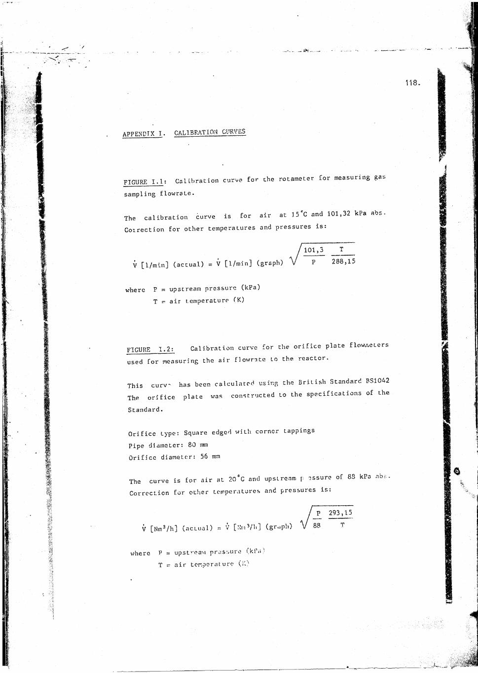
APPENDIX I. CALIBRATION CURVES

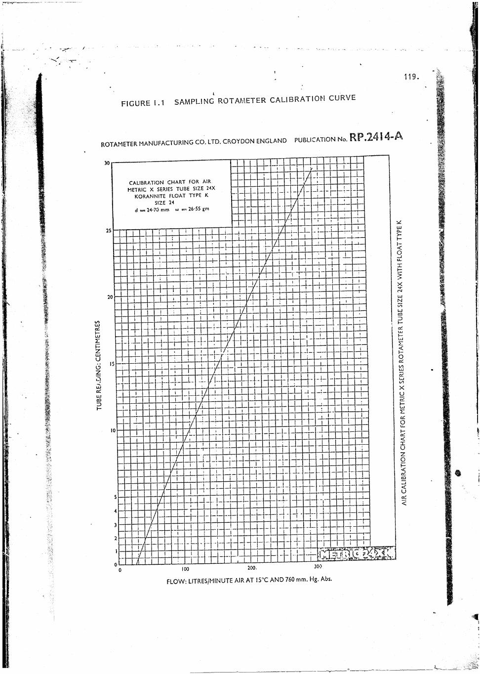
FIGURE 1.1: Calibration curve for the rotameter for measuring gas

sampling flowrate.

The calibration curve is for air at 15*0 and 101,32 kPa absCorrection for other temperatures and pressures is:

101,3 T

V [1/min] (actual) = V [1/min] (graph) V P 288,15

where P = upstream pressure (kPa)T - air temperature (K)

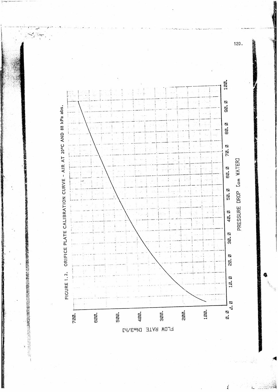
FIGURE 1.2: Calibration curve for the orifice plate flowmeters

used for measuring the air flowrate to the reactor.

This curv- has been calculated using the British Standard BS1042 The orifice plate was constructed to the specifications of the

Standard.

Orifice type: Square edged with corner tappings

Pipe diameter: 80 mm Orifice diameter: 56 mm

The curve is for air at 20*C and upstream p essure of 83 kPa aos.Correction for other temperatures and pressures is.

P 293,15

V [NmS/h] (actual) = V [XmVh] (graph) V 88 T

where P = upstream pressure i.kpa 'T - air temperature

119.

FIGURE 1.1 SAMPLING ROTAMETER C A L IB R A T IO N CURVE

ROTAMETER MANUFACTURING CO. LTD. CROYDON ENGLAND PUBLICATION No.

as

CALIBRATION CHART FOR AIR METRIC X SERIES TUBE SIZE 24X

KORANNITE FLOAT TYPE K SIZE 24

d = 24-70 mm w •=« 26-55 gm

"I

HIP. ?1

3#

FLOW: LITRES/MINUTE AIR AT IS X AND 760 mm. Hg. Abs.

CM/e^Nl 3ivy MOld

121.

APPENDIX II. GRAPHS OF THE OUTPUT CURVES FOR THE_LONG REACTOR

FIGURES II.1 to II.5 : Output curves for runs 1-5 (each "run" is

for a different flowrate - see table 3.1)

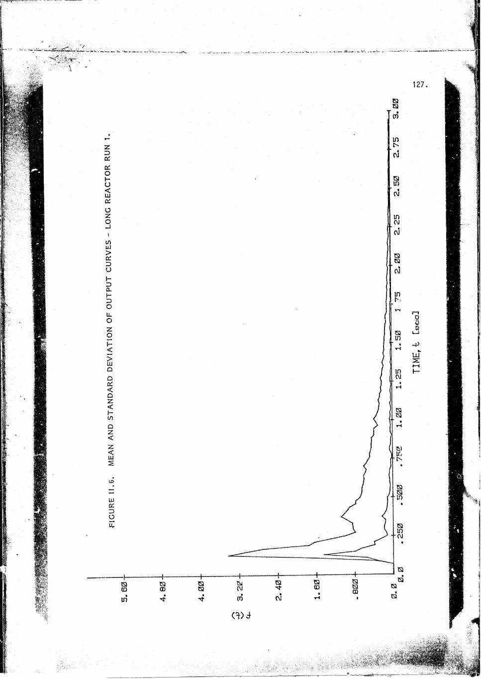
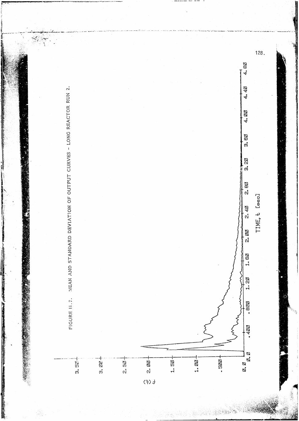
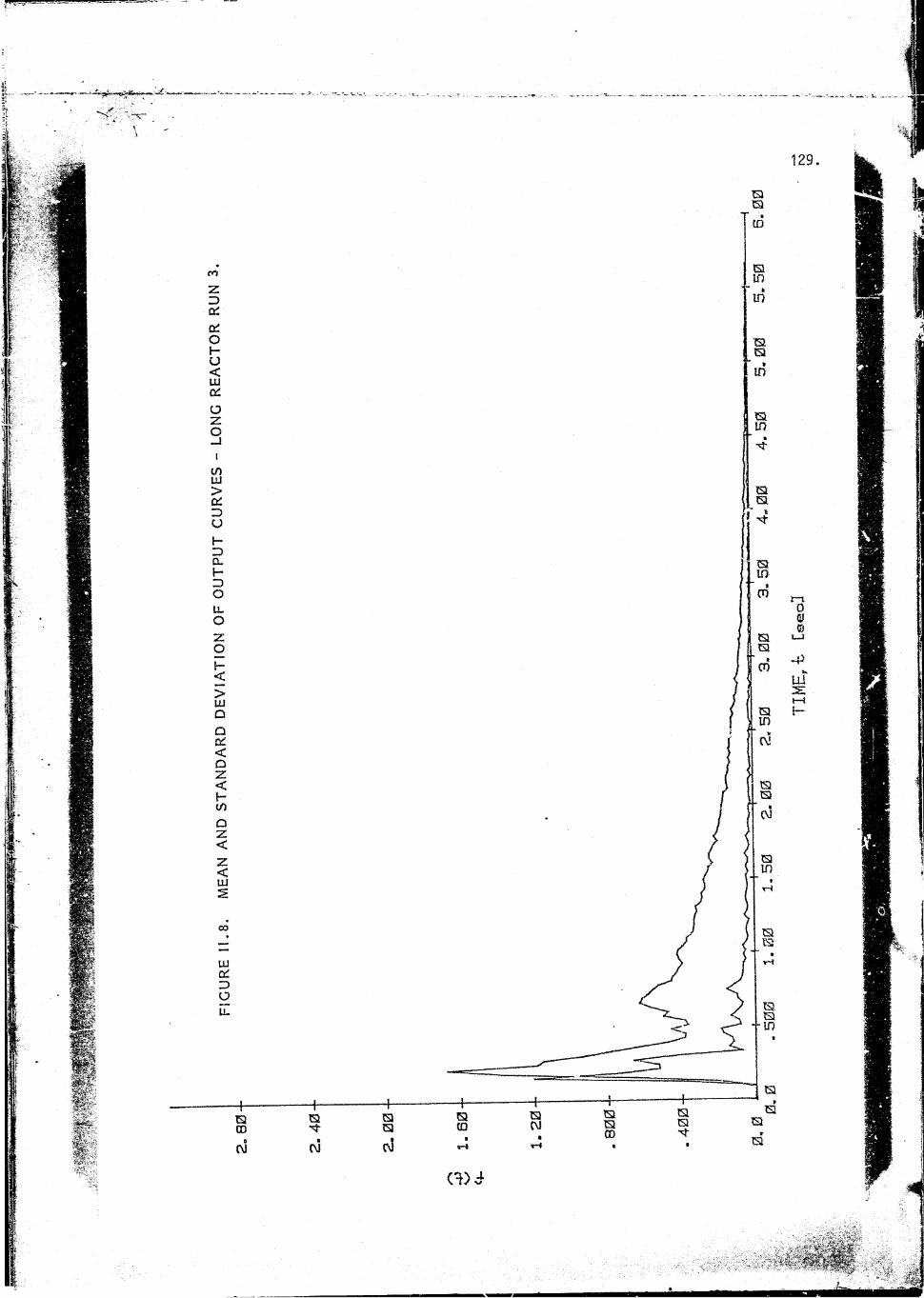
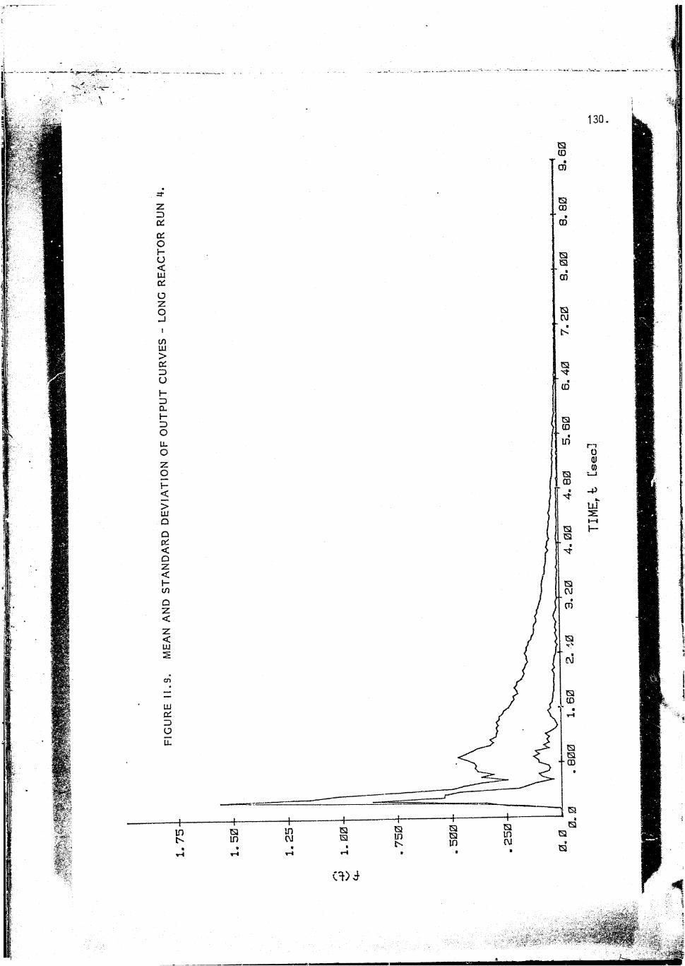
FIGURES II.6 to 11.10 : The mean and standard deviation of the

output curves of each run.

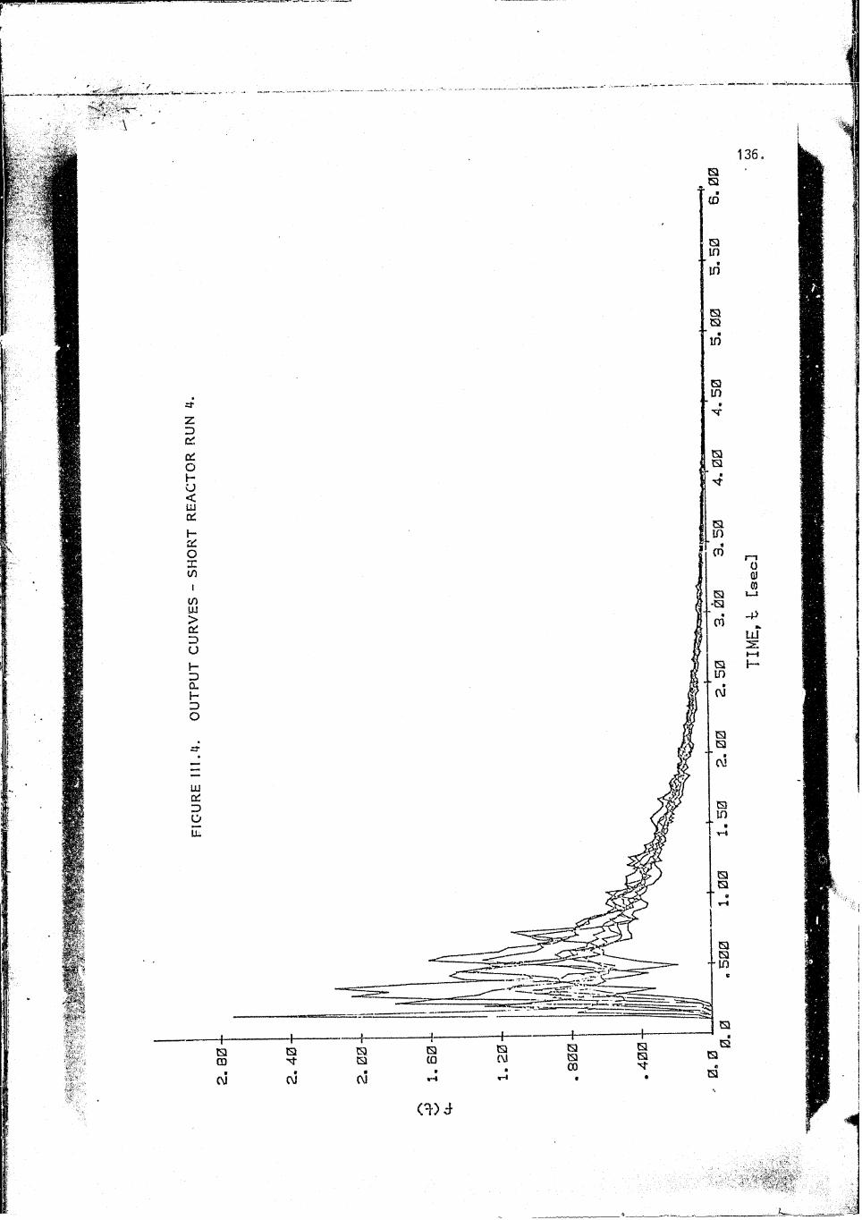
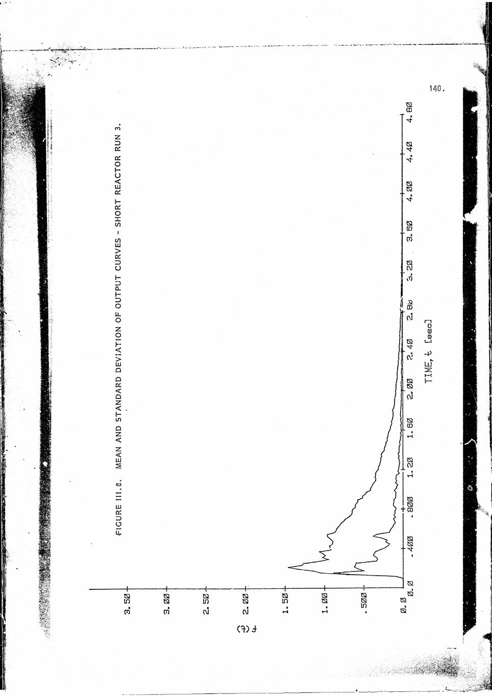
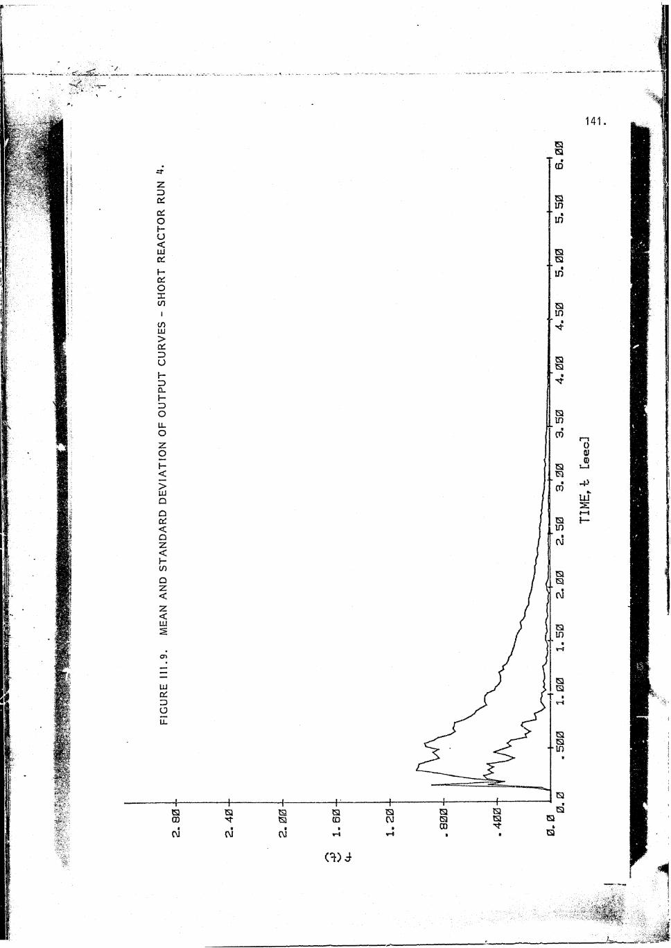
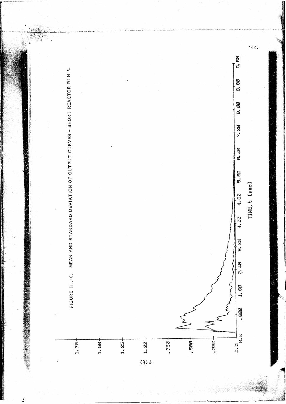
APPENDIX III. GRAPHS OF THE OUTPUT CURVES FOR THE SHORT REACTOR

FIGURES III.I to III.5 : Output curves for runs 1-5 (each "run" is for a different flowrate - see table 3.1).

FIGURES III.6 to III.10 : The mean and stadard deviation of the

output curves of each run.

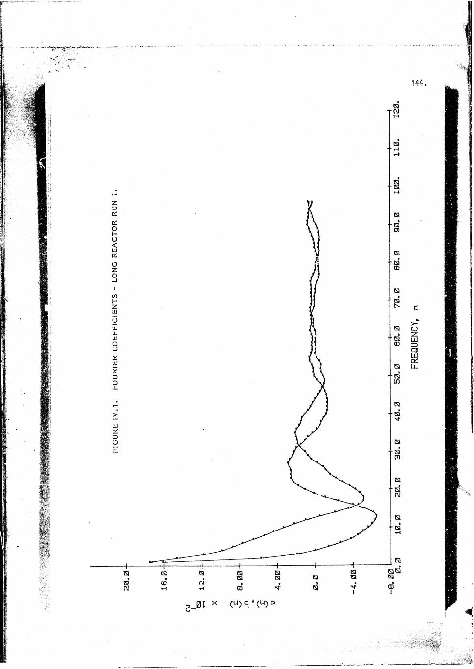
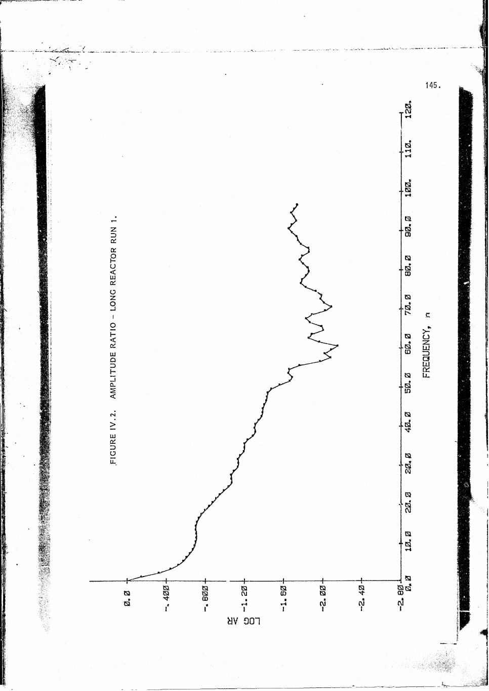
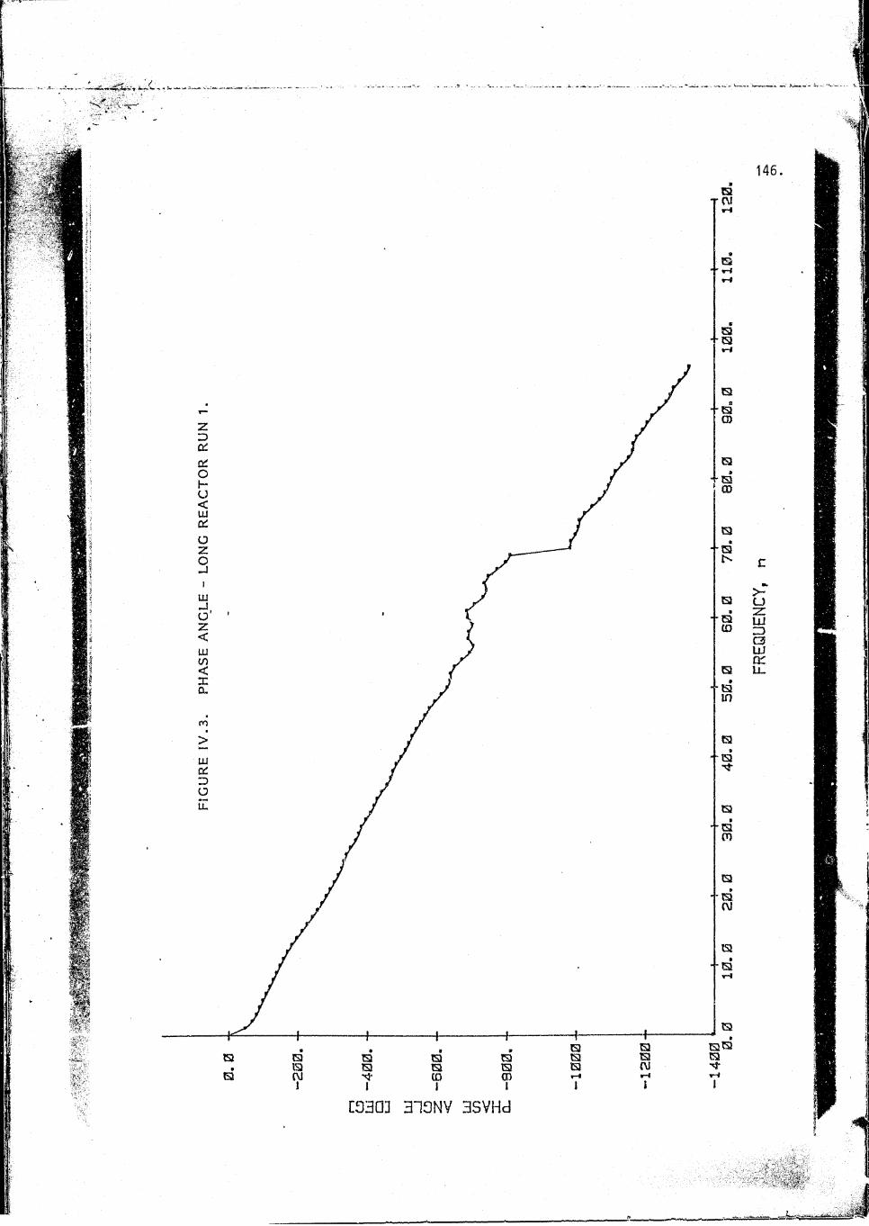
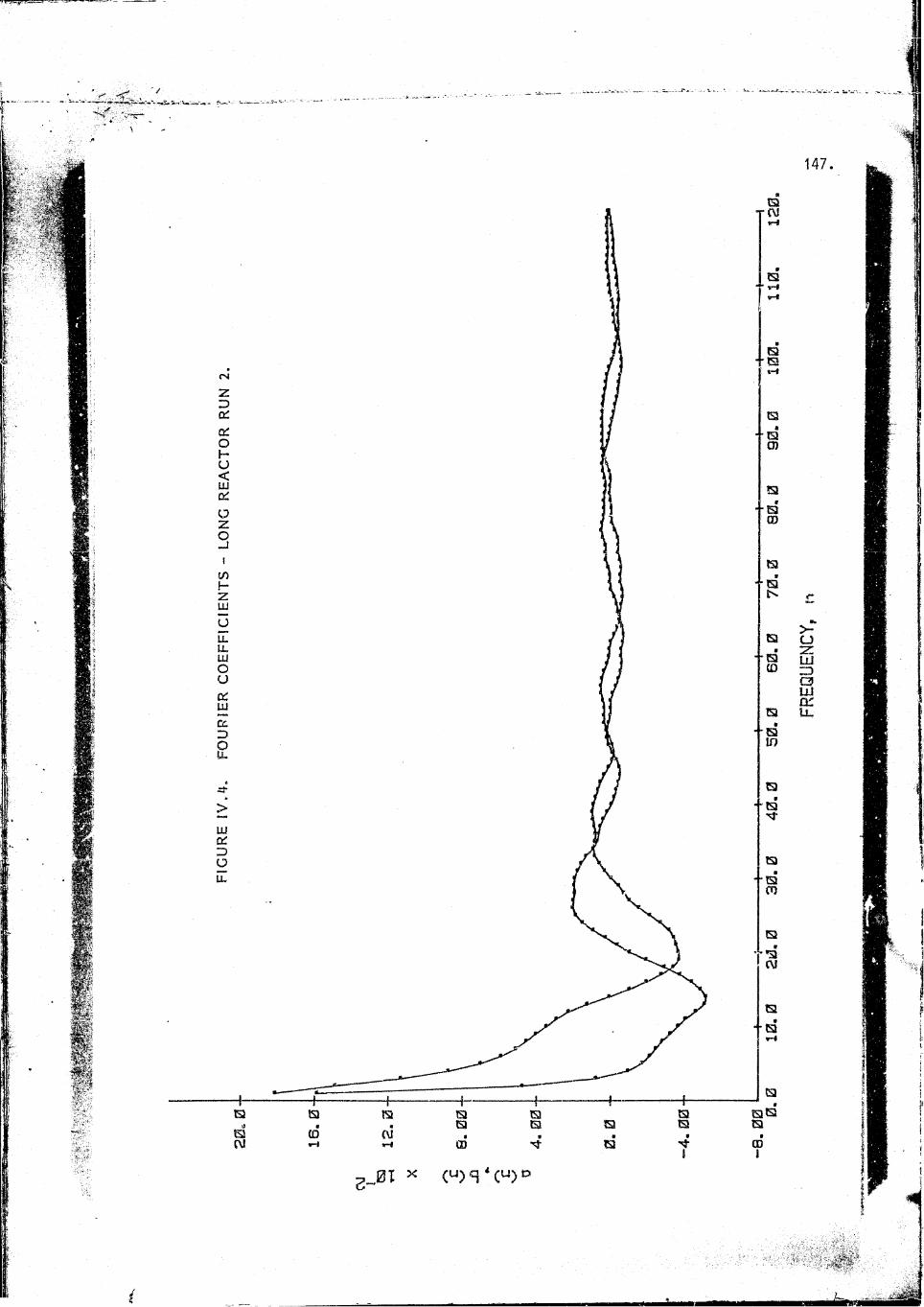
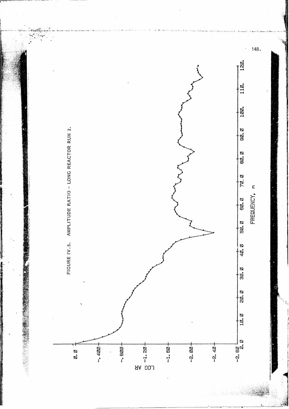
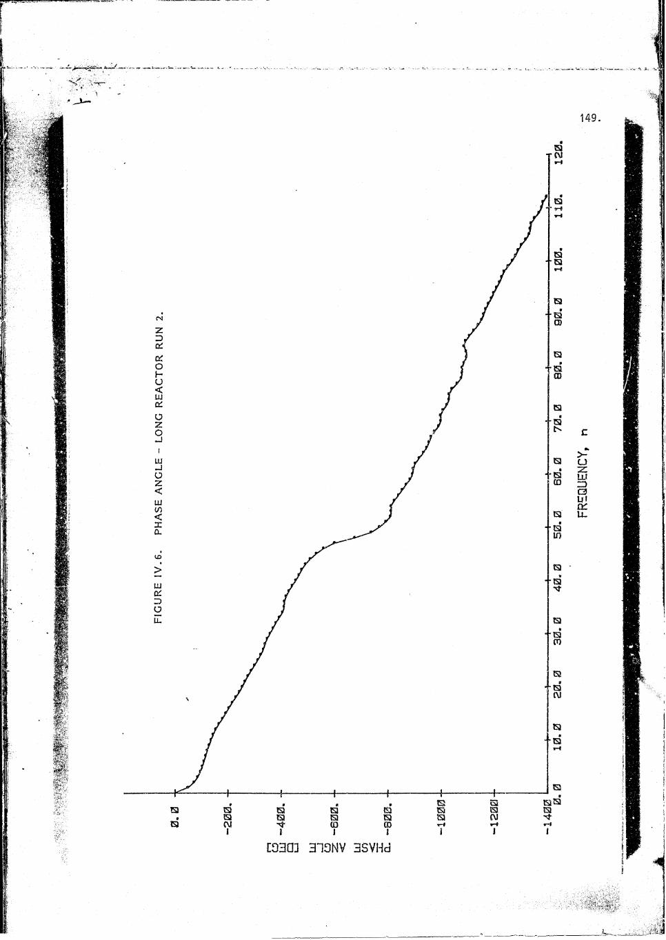
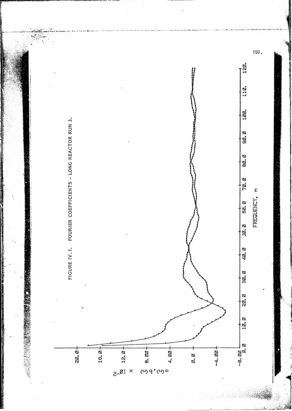
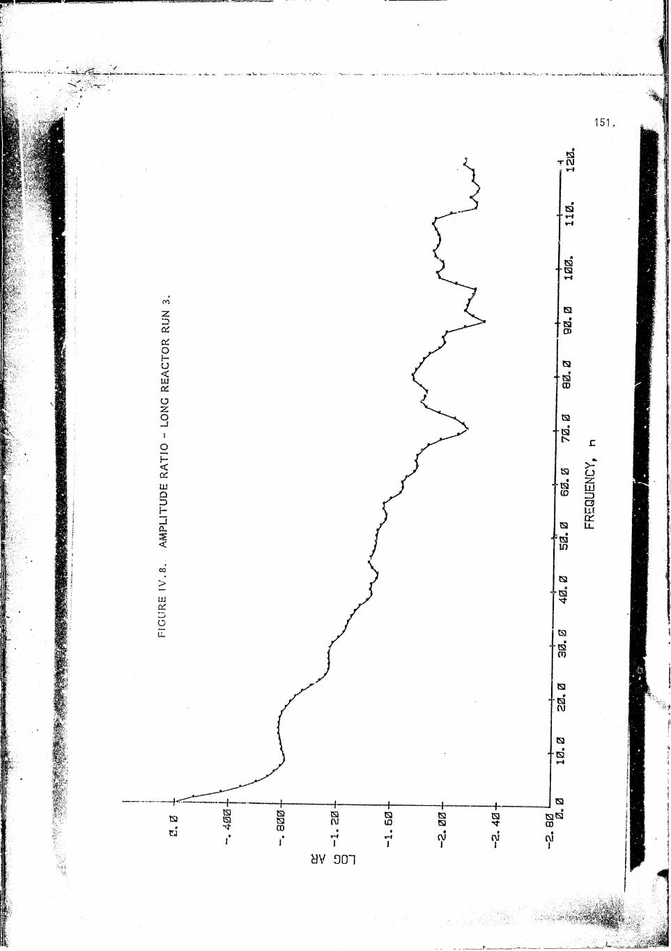
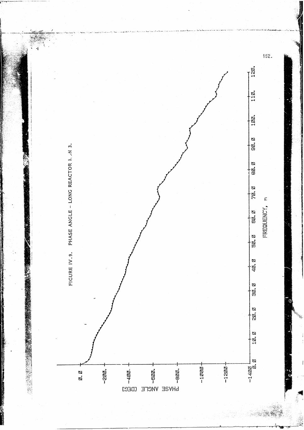
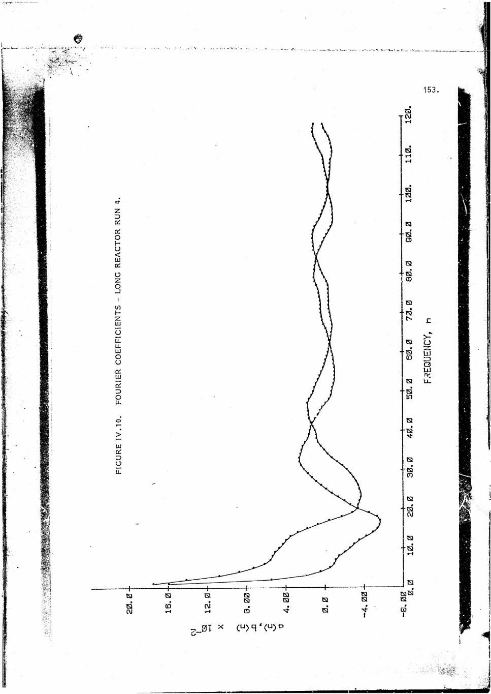
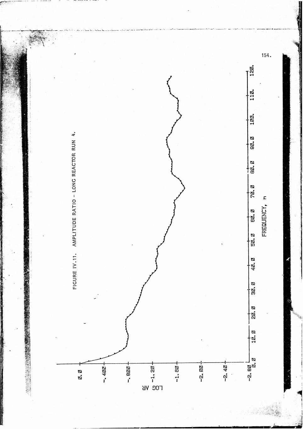
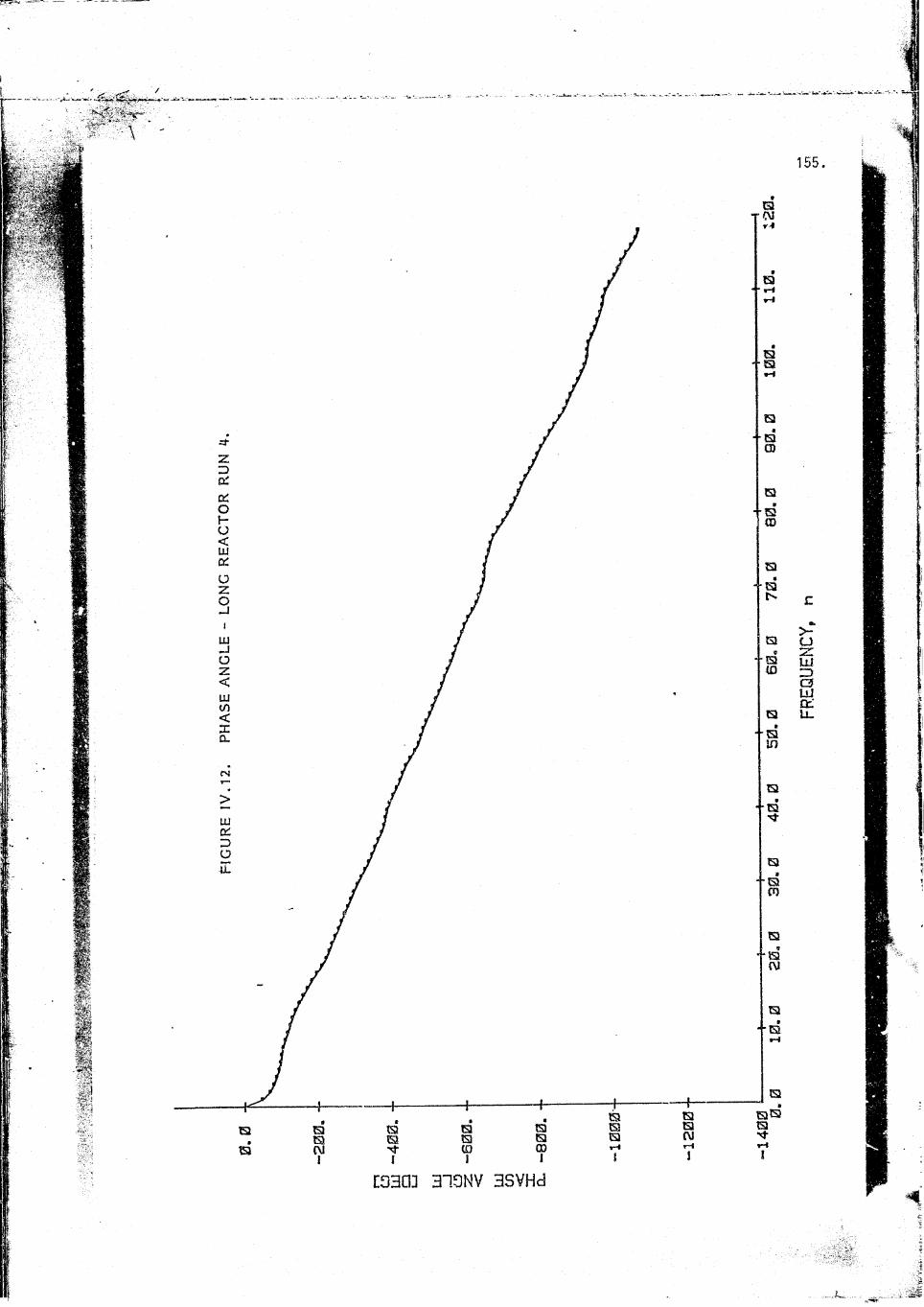
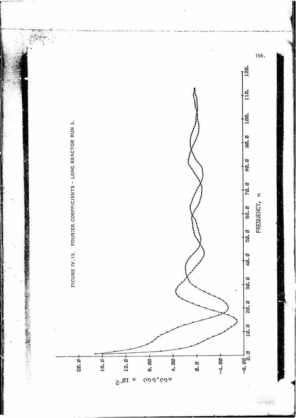
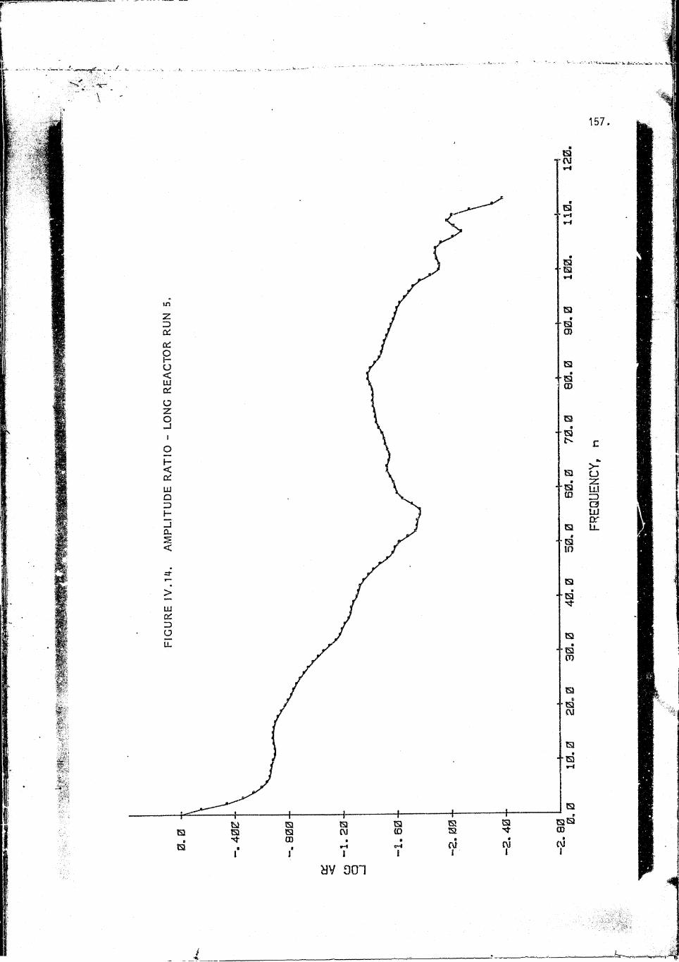
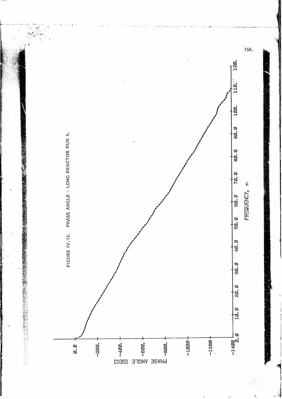
APPENDIX IV. GRAPHS'OF THE FOURIER COEFFICIENTS, AMPLITUDE RATIO AND PHASE ANGLE FOR THE OUTPUT CURVES OF THE LONG REACTOR

.FIG

URE

IV.

2. A

MPL

ITU

DE

RATI

O

- LO

NG

REAC

TOR

RUN

1.

>-UzLUaQ1U.

[330] 313NV 3SVHd

147,

>-CJz:HiZ)so ru_

.0% XCD 't

(U)C|\U)D

[030] 310NV 3SVHd

FIG

URE

IV.9

. PH

ASE

ANG

LE

- LO

NG

REA

CTO

R

k.,N

3.

[030] 310NV 3SVH3

[030] 310NV 3SVH3

r-i

r-6in

co

156,

uzLUZ5£3LU£KU-

p-:.

---- f-------- 1-e

Q S3 tata tatsj CMi i8CD1

csaE3CDI

158.

[330] 313NV 3SVH3

FREQUENCY:

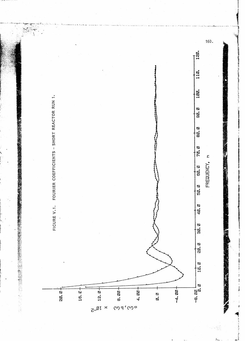
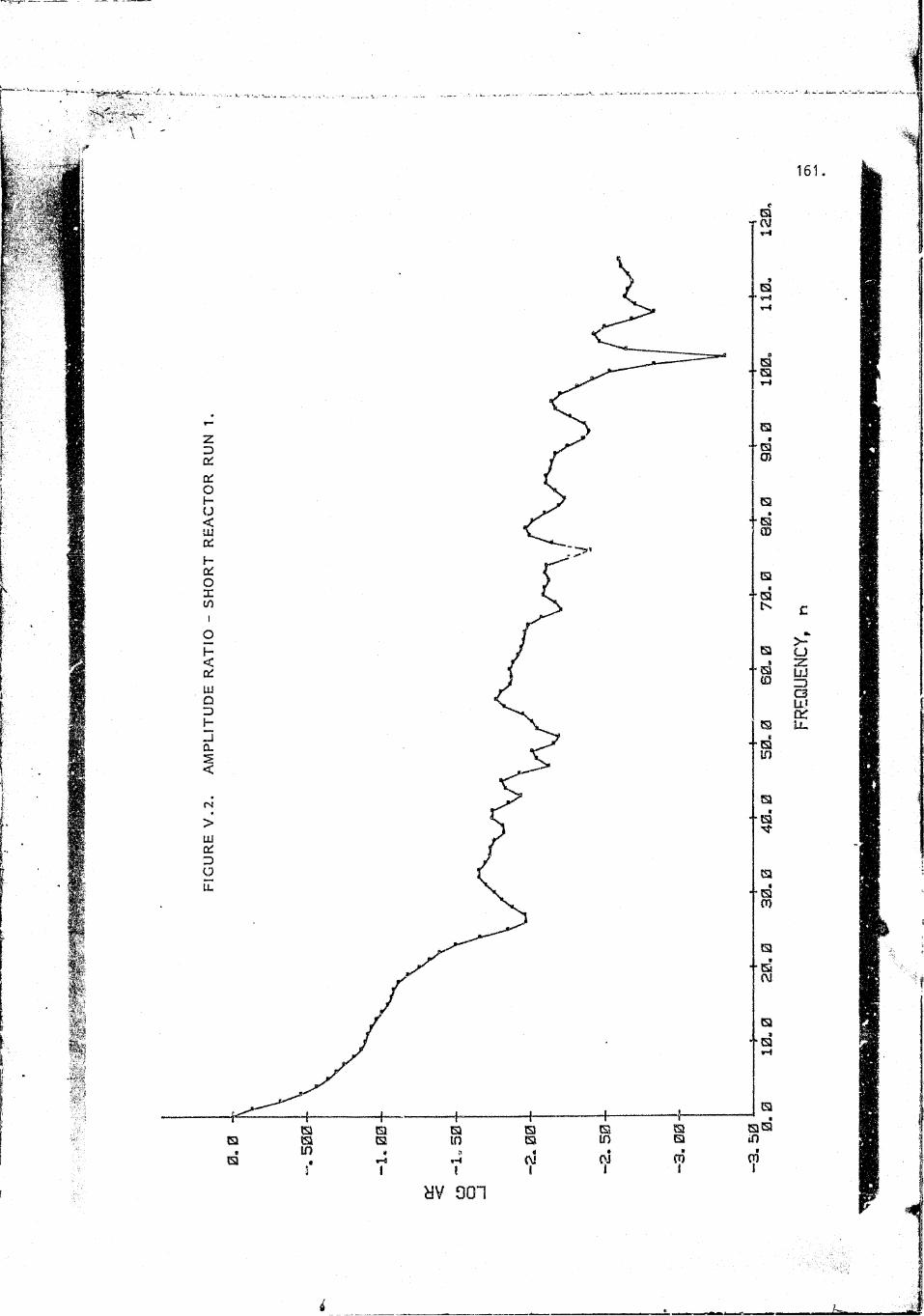
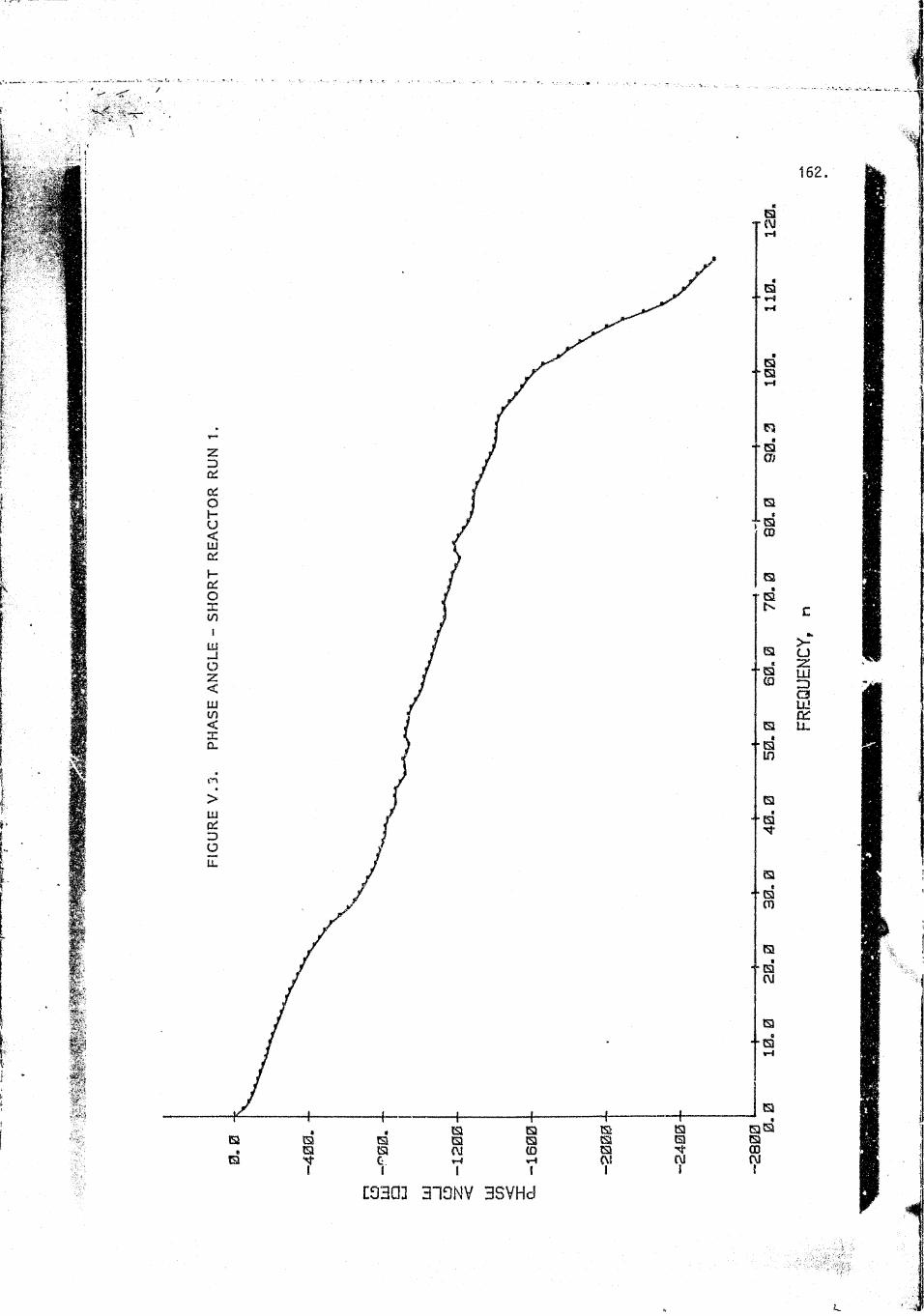
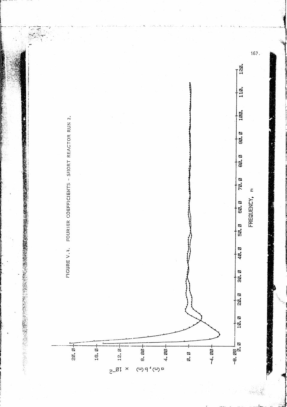
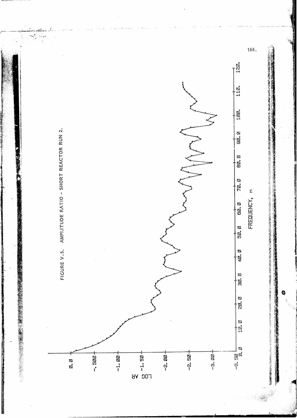
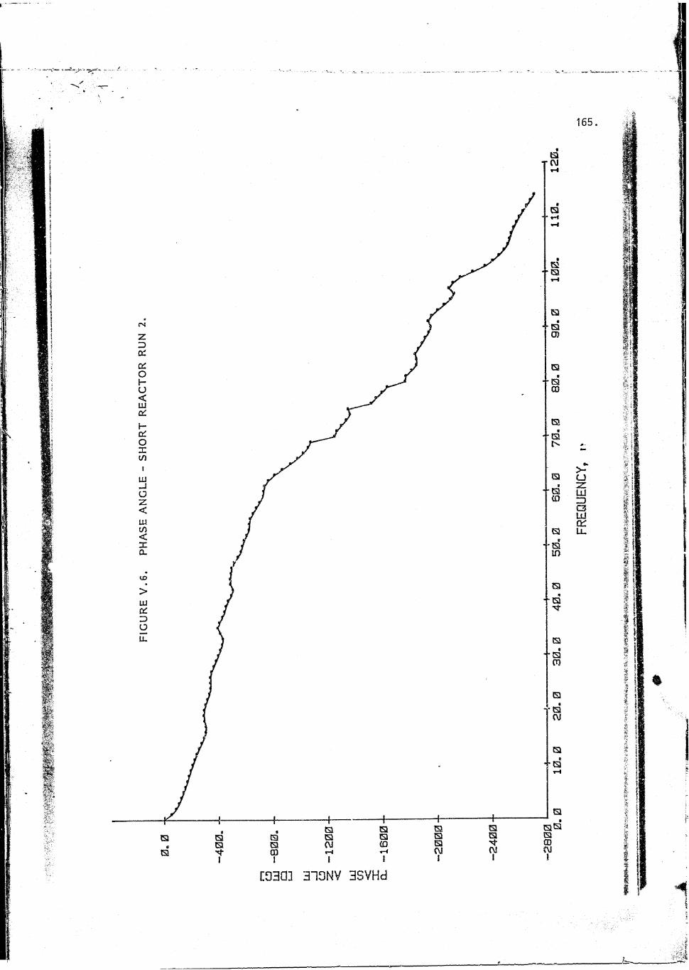
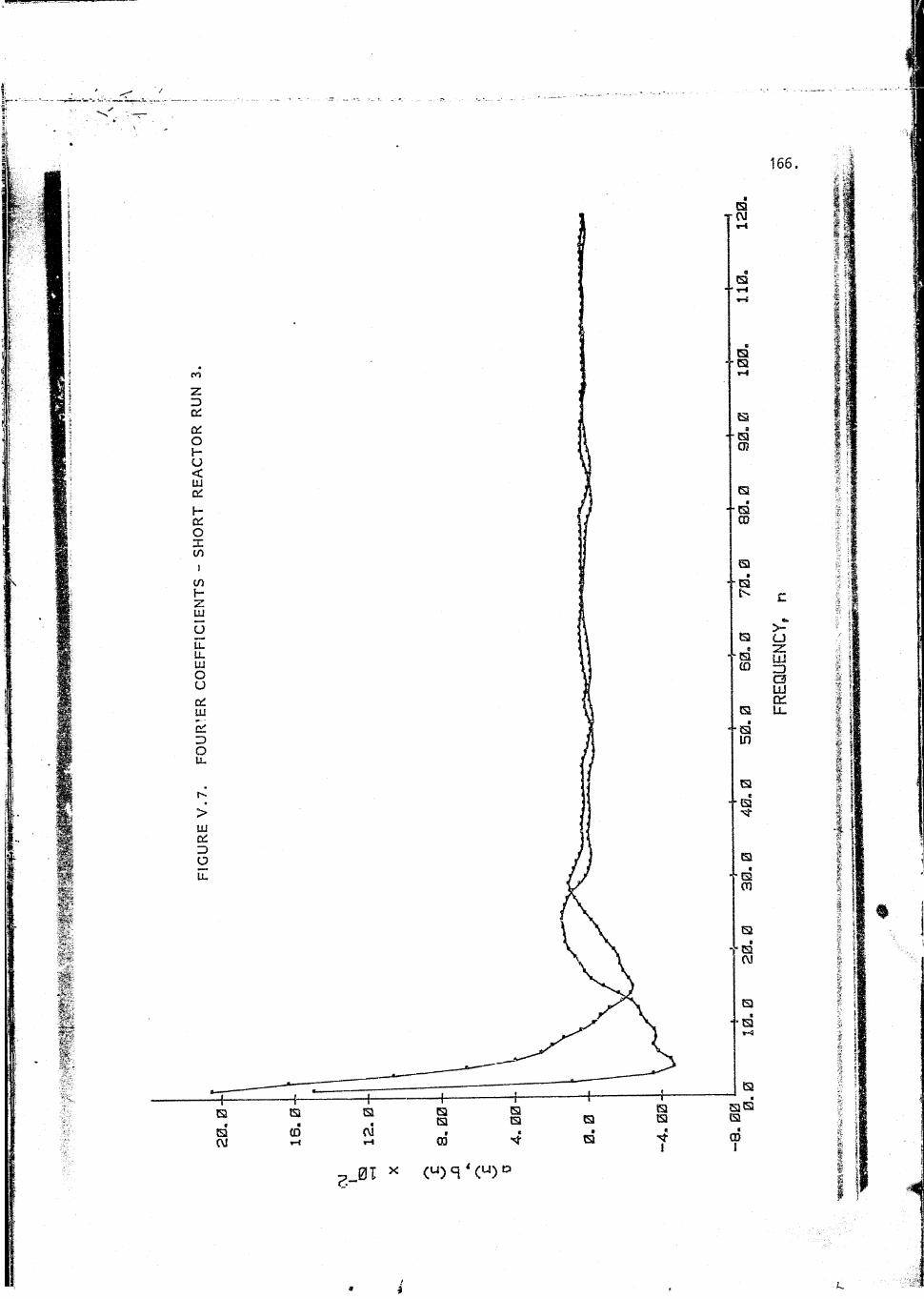
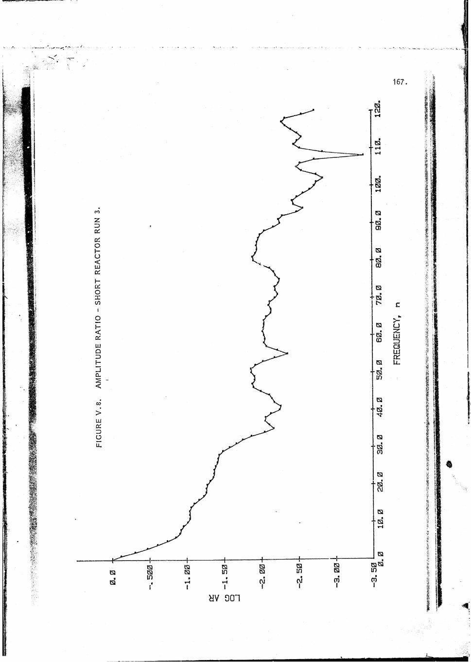
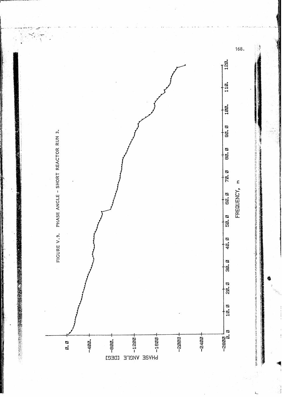
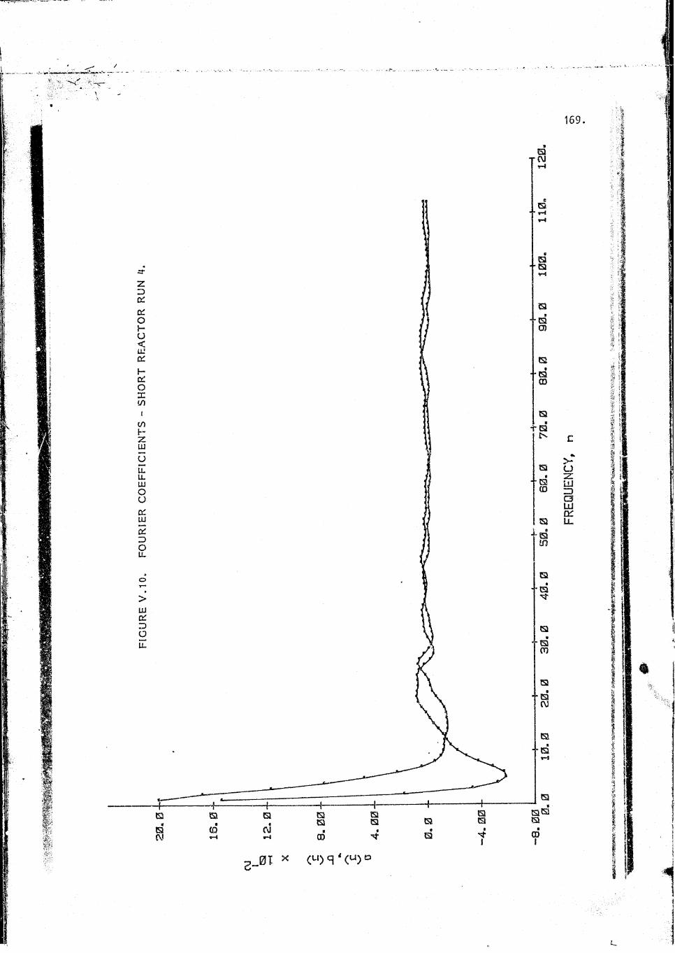
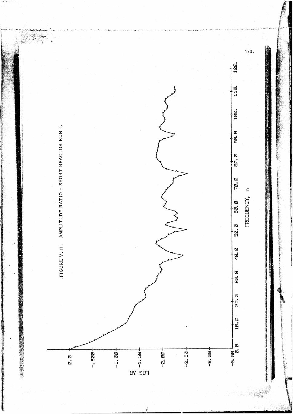
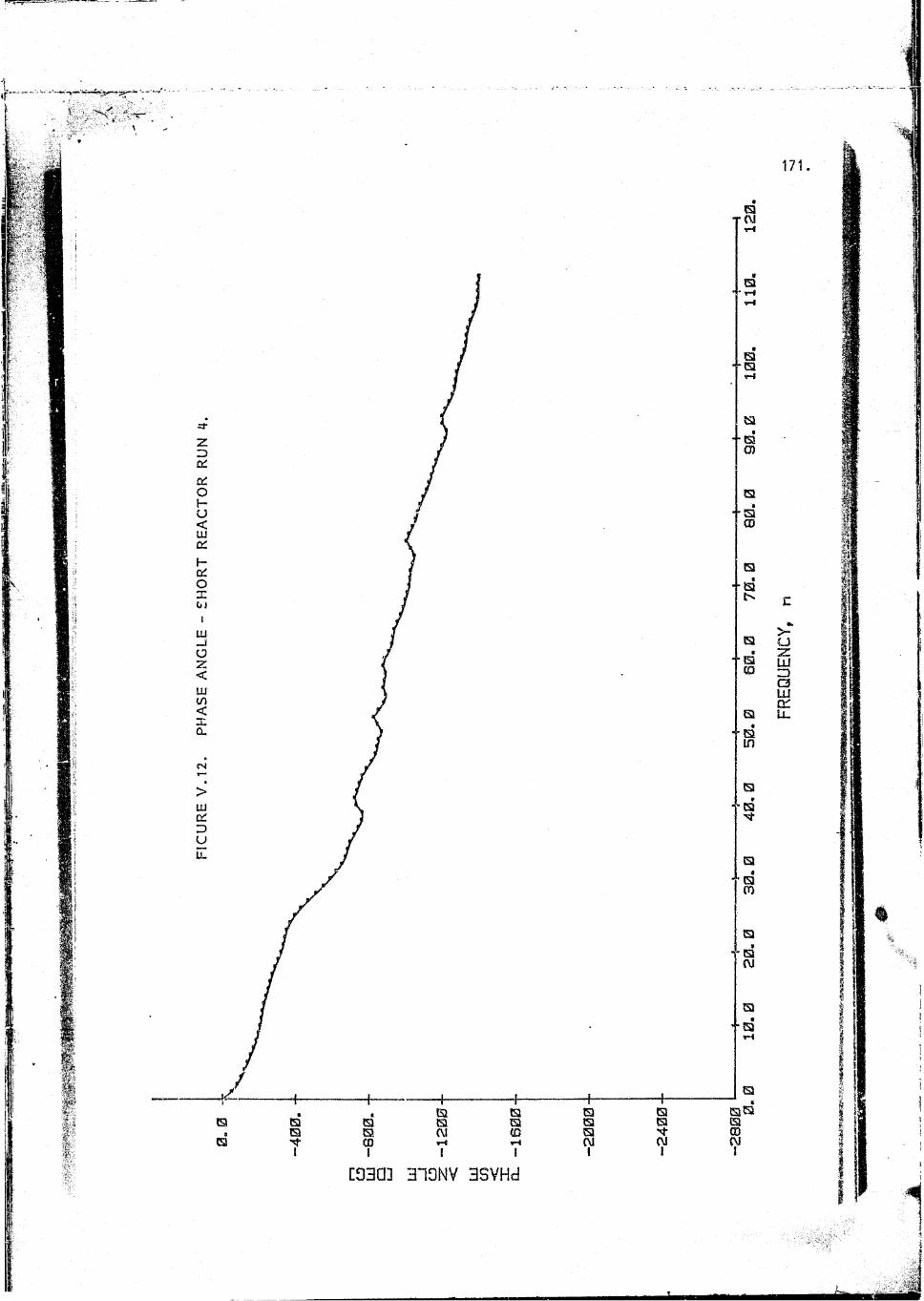
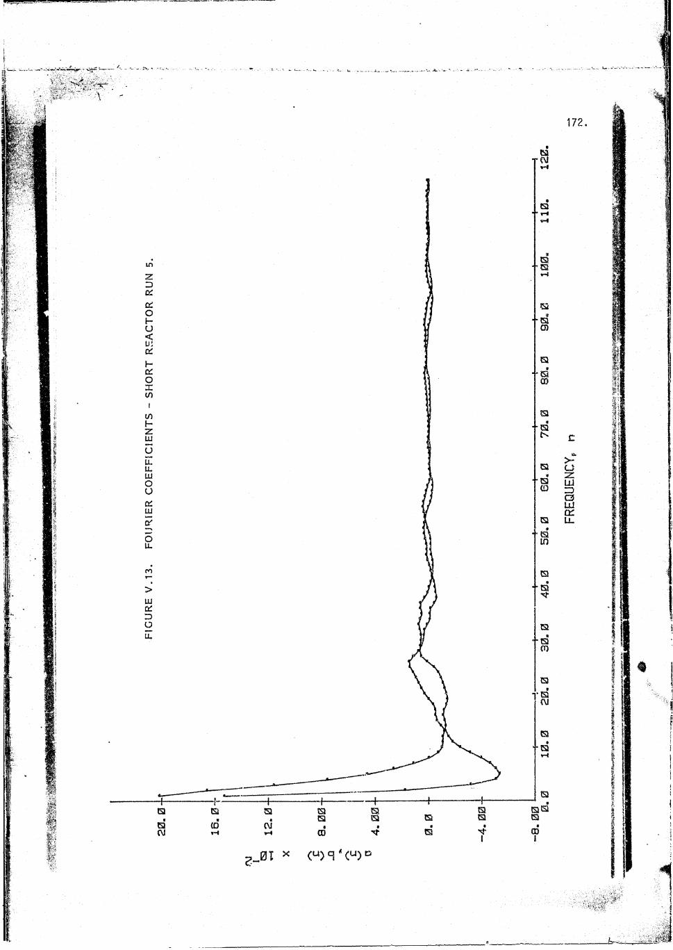
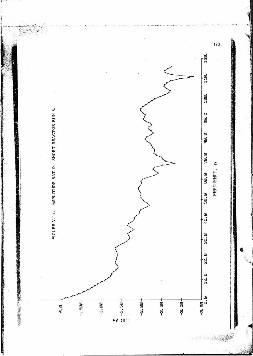
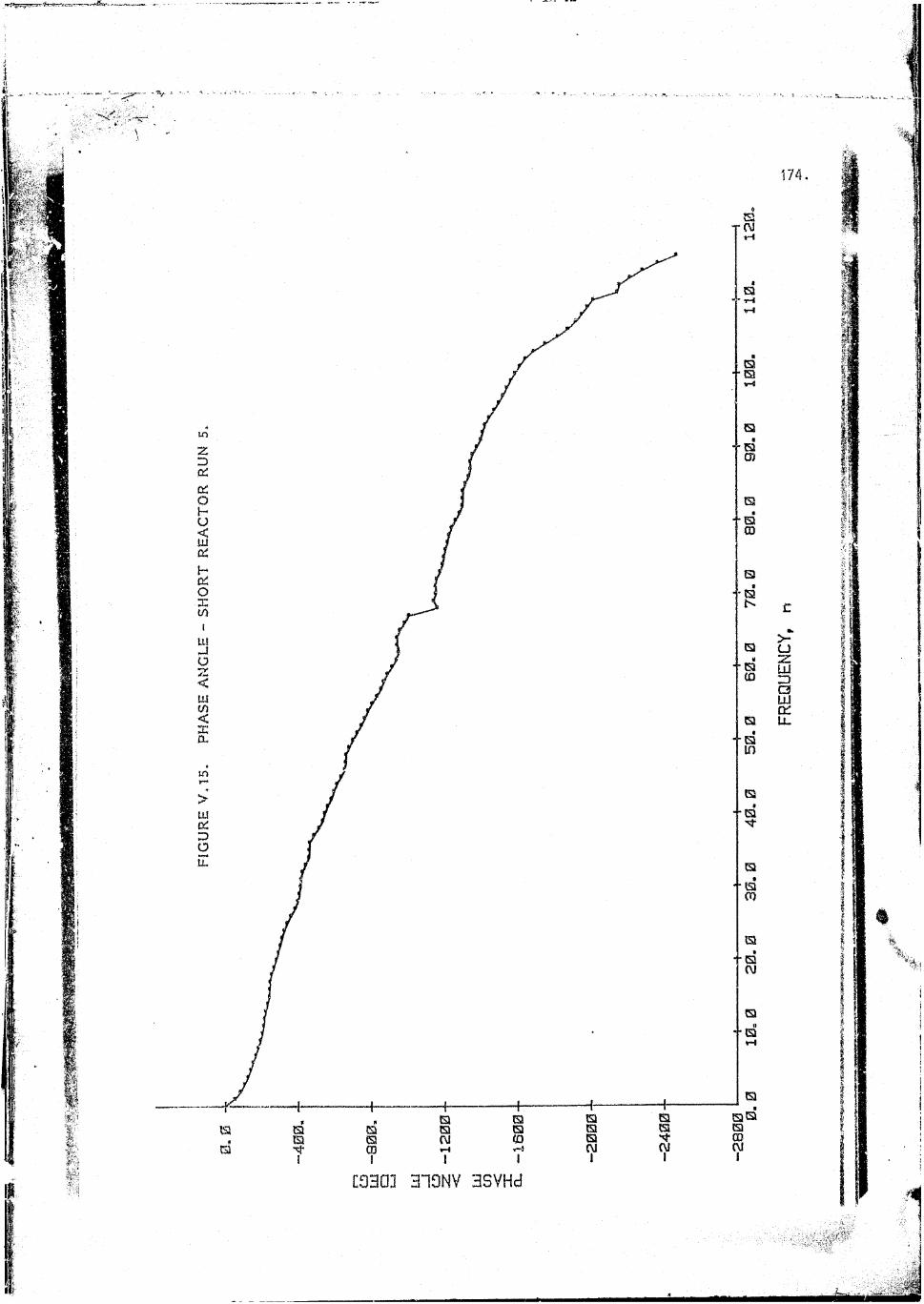
APPENDIX V .' GRAPHS.OF THE FOURIER COEFFICIENTS, AMPLITUDE RATIOAND PHASE ANGLE FOR THE OUTPUT CURVES OF THE 5HQRT__REACTOR

[030] 310NV 3SVHc)

C93Q] 313NV 3SVHd

[030] 310NV 3SVH3

[3303 313NV 3SVHd

[030] 313NV 3SVHd

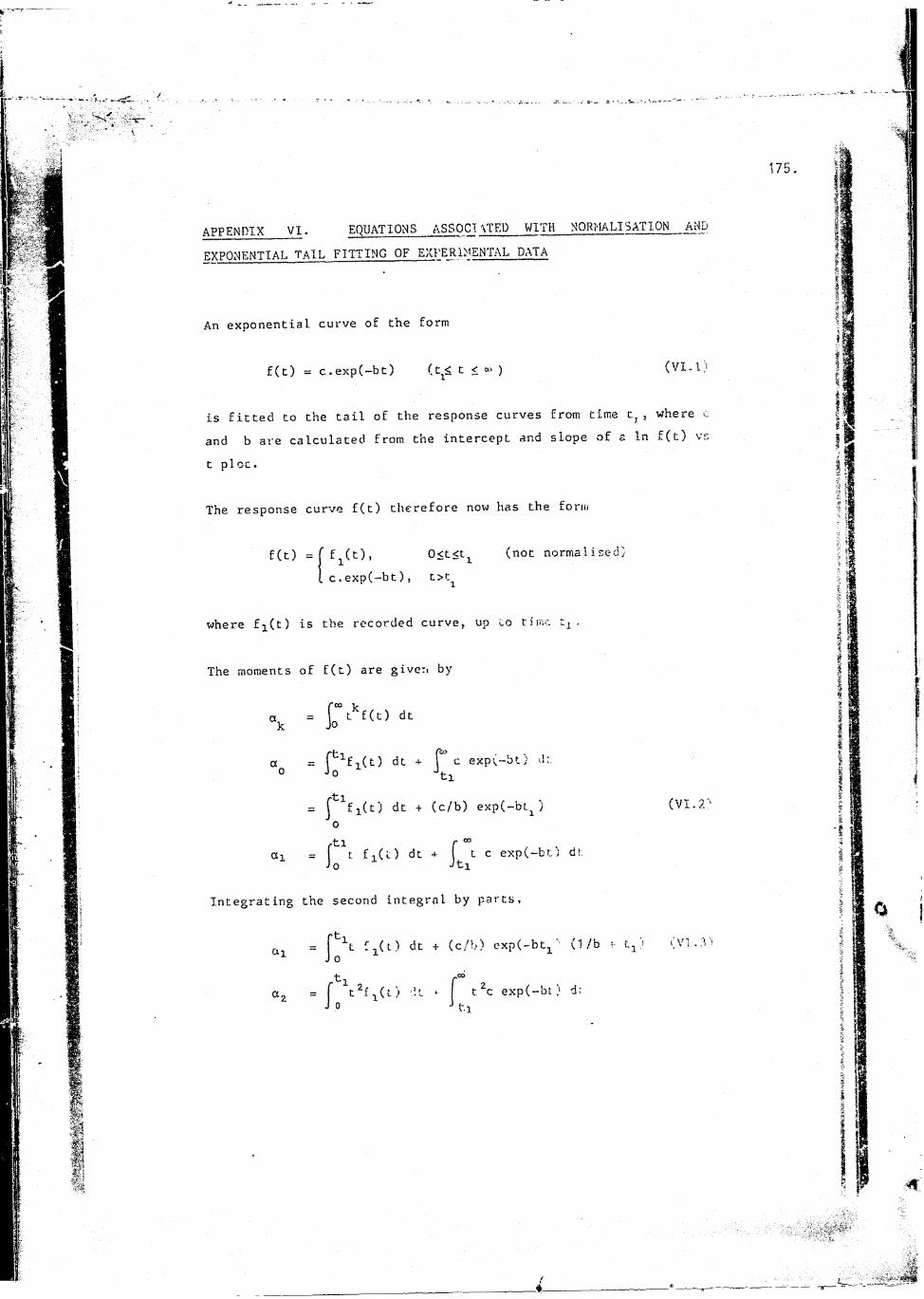
APPENDIX VI. EQUATIONS ASSOC?\TED WITH NORMALISATION AND EXPONENTIAL TAIL PITTING OF EXPERIMENTAL DATA

An exponential curve of the form

f(t) = c.exp(-bt) (t^ t < » ) (VI-1.

is fitted to the tail of the response curves from time t,, where iand b are calculated from the intercept and slope of s In f(t) vst plot.

The response curve f(t) therefore now has the form

f(t) f (t), 0<t<t1 (not normalised;. c.exp(-bt), t>Cx

where f%(t) is the recorded curve, up to time tj .

The moments of f(t) are giver cr

“k =fca t,( t f(t) dt

ao = ftifi(t) dt +J 0 . . . . i c expt-bt/ dr.

ti

= j fi(t) dt + 0 (c/b) exp(-bti )

Oi =ztlf t fi(l) dt Jo

r 00+ 1 t c exp(-bt) dt

Jti

(VI.2:

Integrating the second integral by parts.

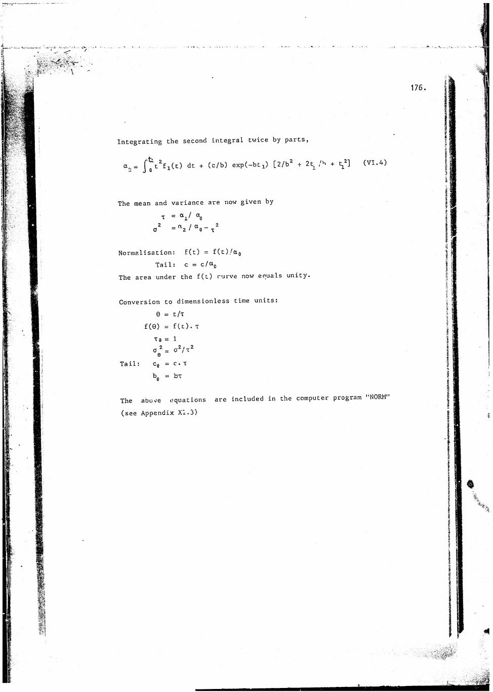
Integrating the second integral twice by parts,

a„ = j* Lt2'f1(t) dt + (c/b) exp(-bti) [2/b2 + 2t /h + t 2] (VI. 4)

The mean and variance are now given by

T = *oO2 = nz / “ o - T2

Normalisation: f(t) = f(t)/a0Tail: c = c/a0

The area under the f(t) curve now equals unity.

Conversion to dimensionless time units:9 = t/T

f(6) = f(t).T T 9 = 1 0 2 = 02/t2e

Tail: ce = c. T

be = bT

The abo^e equations are included in the computer program "NORM"

(see Appendix XI.3)

APPENDIX VII. TIME DOMAIN SOLUTIONS AND MOMENTS— FOR— THE

MATHEMATICAL MODELS

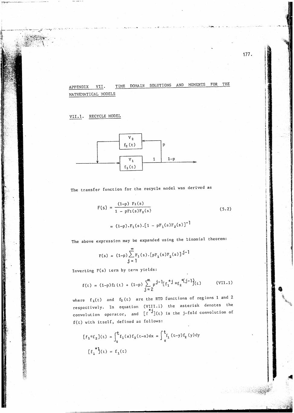
VII.1. RECYCLE MODEL

v2f2(c)

s

p

1-p............f Vifl(t)

1

The transfer function for the recycle model was derived as

(1-p) Fi(s)~ 1 - pFi(s)F%(s) (S'?)

= (1—p).Fx(s)-[1 — pF1(s)F2(s)]Fhe above expression may be expanded using the binomial theorem:

F(s) = (1-p) 5Z 3 (s).[pF1 (s)F2(s)]^"j = l

Inverting F(s) term by term yields:

f(t) = (i-p)fi(t) + (i-p) Z p ^ k f ^ (vii.i)j = 2

where fi(t) and fzft) are the RTD functions of regions 1 and 2 respectively. In equation (VIII.1) the asterisk denotes the convolution operator, and [f*J](t) is the j-fold convolution of

f(t) with itself, defined as follows:

[fx*f2](t) = rtfi(x)f2(c_x)dx = j \ ( t - y ) f 2 (y)dyn 0

178.

} - F 1(s)F2 (5 )

The terms of equation (VII.1) have a physical significance as they represent the RTD functions of material that has passed j times

through the system.

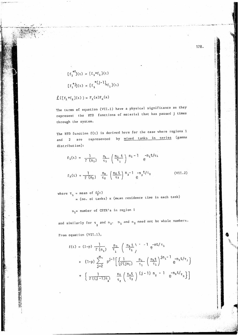
The RTD function f(t) is derived here for the case where regions 1and 2 are represented by mixed tanks in— series (gamma

distribution):

rti / n i t \ D i - l - D i t / t i

£ - l “ )

Dg / n z t \ n ^ - l ( v i i . 2 )Tz \ Tz / e

where = mean of f^t)= (no. of tanks) x (mean residence time in each tank)

f;(t) =

"z(t)

ITTni)

1Tni)

number of CSTR's in region 1

and similarly for and n,. n^ and n, need not be whole numbers

From equation (VII.1).

f(t) = (1-p) — 1 ni n1 t \ ' -1 - n t / x ,— 4— p

(VP) H 3=2

r i _

r(jni)n i t V ni " 1 -n1t/-cJ}

H lTn

n , t \ (d - 1) n - 1 "n2t /^ 2)

f(c) - d-p) ^

x— i-1 ] 1 f l l ^2( V p ) Z p T U T ) T « F T ) V \ -

j= 2 1

j " i - n . x / T j n ^ t - x i f - ^ V e-n2(t-(VII.3)

. ' 6 1 ' '

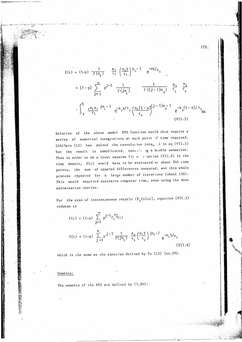
Solution of the above model RTD function would thus require a series of numerical integrations at each point of time required. Gibilaro (12) has solved the convolution inte^ .1 m eq (VII.3) but the result is complicated, cont V.. ig a double summation. Thus in order to do a least squares fit o r ualion (VII.3) m the time domain, f(t) would have to be evaluated at about 240 time points, the sum of squared differences computed, and this whole process repeated for a large number of iterations (about 150). This would required excessive computer time, even using the best

minimisation routine.

For the case of instantaneous recycle (F2(s)=l), equation (VII.3) reduces to

COf(t) = (1-p) Z pj"Tf*j(l:)

j=l

f(0 = (1-p) rljiT ^ ("t7 ) J"’ 1 e'"lt/T‘(VII.4)

which is the same as the equation derived by Fu (13) (eq.29).

Moments:

X)/T%dx

The moments of the RTD are defined by (7,20).

and may be obtained from Che transfer function as follows :

\ = ( - 1>ki r ( s ) U < v n -6>

The mean and variance of f(t) are defined as

t = 01/ aQc 2 - a 2 /a0 - T 2 <V I I '8)( a = 1 for an RTD curve)

(VII.7)

and can be calculated as follows:

T < V I I - 9>

02 = In FCs)! (VII.10)ds2 s 0

For the recycle model (with any half loop RTDs):

In F(s) = In (l-p)Fi(s) - In (1 - pFi(s)F 2(s)In F(s)=Fi(s) + p[Fx(s)F2(s) + Fx(s)F?.(s)

Fi(s) 1 - pFx(s)F2(s) (VII.11)

where the prime indicates differentiation.

ds Fi(s)Z

p[l - pf,(s)%,(s)][Pi(s)F2"(s) + Fj(s)F&(s) + Fi(s)F2(s) + Fi"(s)%(s):[1 _ pFi(s)F2(s)l 2

P=[F\(s)F^(s) + F'(s)F2(s)][Fi(s)F^(s) + r[(s)Fg(s)][l - pFi(k)F2(5)]2 (VII.12)

181.

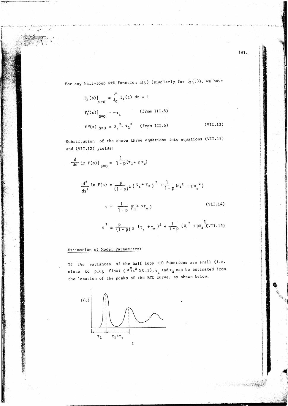
For any half-loop RTD function fiU) (similarly for f2 (t)), we haveFi (s) | = [ fx (t) dt = 1

S=0 0S=0

F "( s ) | s=o

= -T, (from III.6) (from III.6) (VII.13)

Substitution of the above three equations into equations (VII.11)

and (VII.12) yields:

d _L-ar-ln F ( s ) | ^ = 1- p(Ti+ pTz)

5 ln F<s) = n ^ = i » (T^ T2)2 ^ + p 0 22)

(VII.14)

20 {*rrp) 2 (?! +T2 + T^P Xvii.15)

Estimation of Model Parameters:

If the variances of the half loop RTD functions are small (i.e. close to plug flow) ( e ^ 2 5 0,1), and can be estimated from the location of the peaks of the RTD curve, as shown below:

182.

The recycle fraction p can then be found from equation (VII.14) (where t is calculated by numerical integration of the RTD curve; T equals unity for normalized curves). Also, the area under the first peak should equal 1-p* Furthermore, Oj2 can be estimated by examining the shape of the first peak, and cJj. can subsequently be calculated from equation (VII.15).

The method described above eliminates the need to determine higher order moments and is preferable to the method of moments.However, when the half loop variances are not small (as is thecase in this work), the successive peaks overlap and are not assymmetrical, and only rough estimates of t and can be obtained

by this method.

183.

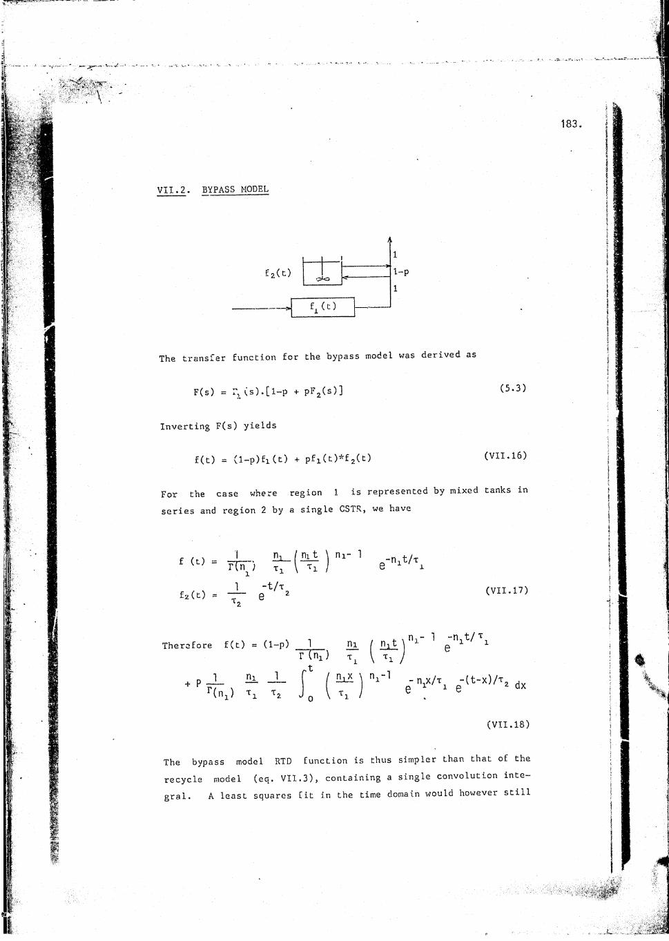
VII.2. BYPASS MODEL

h

1

The transfer function for the bypass model was derived as

F(s) = r^(s).[l-p + pFgXs)] (5.3)

Inverting F(s) yields

f(t) = (l-p)fl(c) + pfl(t)*f2(t) (VII.16)

For the case where region 1 is represented by mixed tanks inseries and region 2 by a single CSTR, we have

(VII.17)

Therefore f(t) = (1-p) 1n

+ Pr(ll1) T1 t2 e-n1x/Ti e-(t-x)/T2 dx

0(VII.18)

The bypass model RTD function is thus simpler than that of the recycle model (eq. VII.3), containing a single convolution inte-gral. A least squares fit in the time domain would however still

184.

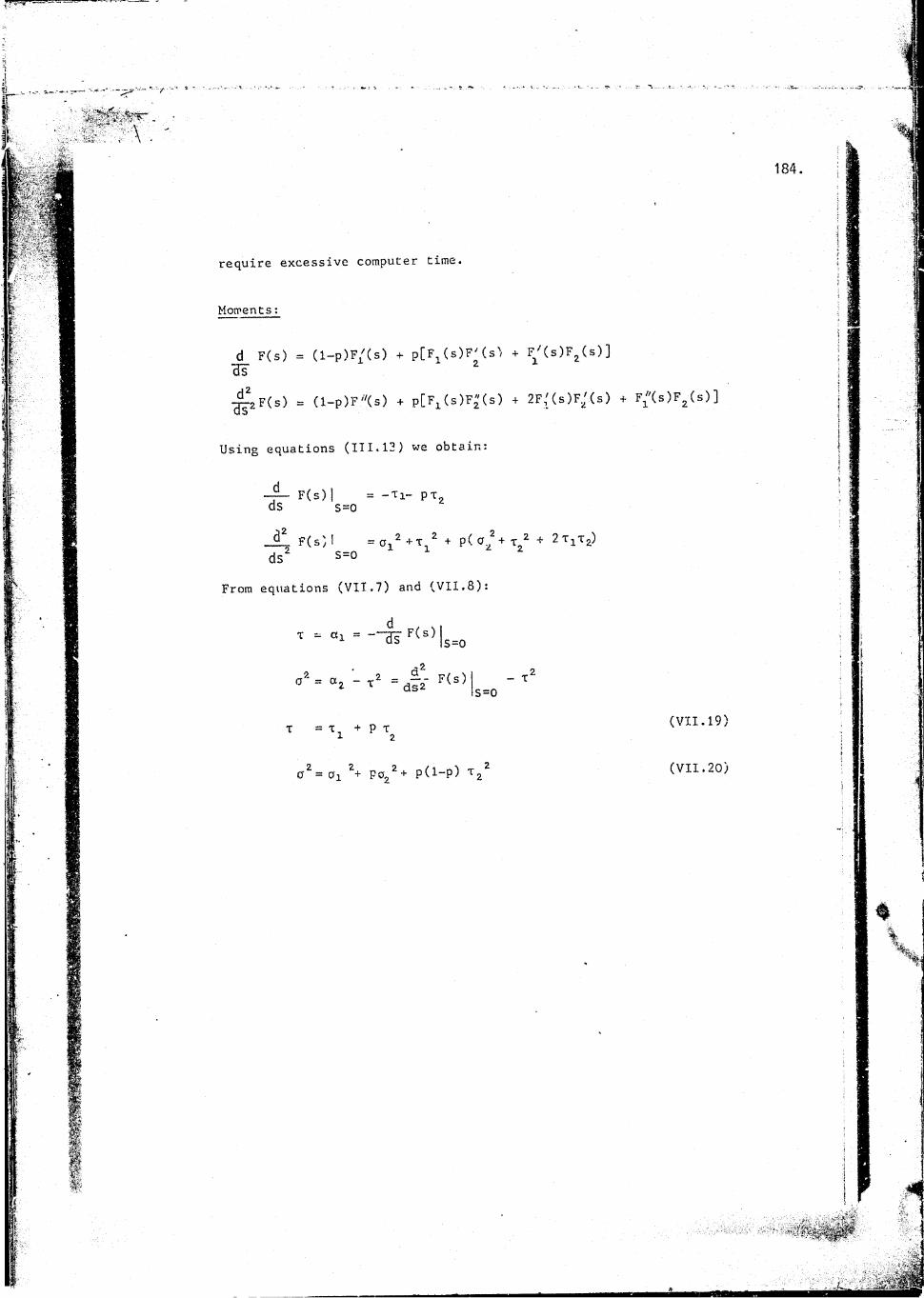
require excessive computer time.

Moments:

d F(s) = (l-p)F/(s) + p[F (s)F'(s^ + F'CsiF^fs)]3s *

= (l-p)F"(s) + p[Fi(s)F;(s) + 2F{(s)F;(s) +

Using equations (111.12) we obtain:

— F(s) I = -Tl- pt2ds s=o

^ F ( s ) l _ = O i * + T \ * + p ( o J + T ^ds" s=o

From equations (VII .7) and (VII.8):d

T = «1 = — 3s F(:)|s=od2 X _2- X

S=0

F^(s)F2(s)]

(VII.19)

185.

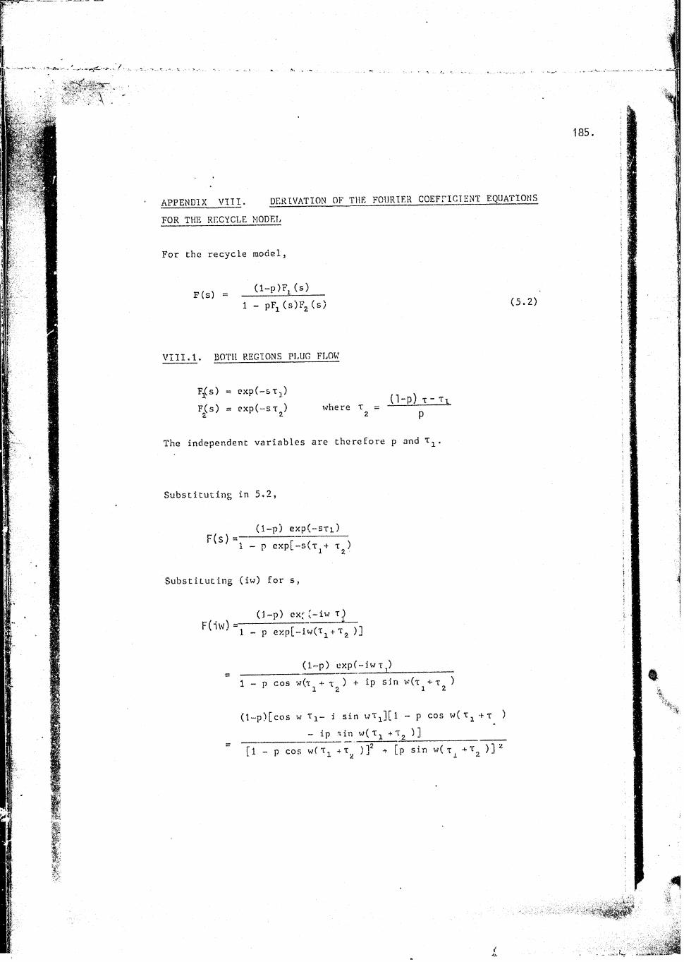
APPENDIX VIII. DERIVATION OF THE FOURIER COEFPICIENT EQUATIONS

FOR THE RECYCLE MODEL

For the recycle model,

p(s) = d-P)Vs.)__1 - pFi(s)Fz(s) i5-2)

VIII.1. BOTH REGIONS PLUG FLOW

FjCs) = exp(-STj) ( l - p J x - T ,F(s) = exp(-sT ) where x = ~2 2 2 p

The independent variables are therefore p and x^.

Substituting in 5,2,

(1-p) exp(-sxi)1- p exp[-s(x1+ x )

Substituting (iw) for s ,

(1-p) cxf(-iw xj F(iw)=i _ p expC-iwfXi + x^)]

(1-p) exp(-iwx^) ______1- p cos w(t1 + x ) + ip sin w(x^ + x^ )

(1-p)[cos w xx- i sin w x 1)[ 1 - p cos w(x1 +x )- ip sin w( x1 + Xg )]_________ _

[1- p cos w( x1 4 xz )]2 + [p sin w( ta +T2 )] z

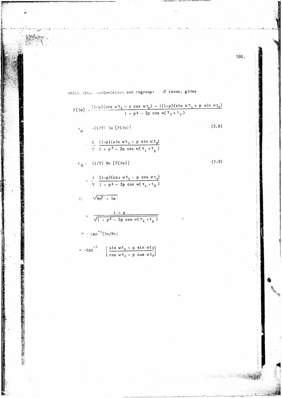
which itrcu ;.:a:iipulmcio:t and regroupi ;f terms, gives

F(iw) =(l-p)(cos wti - p cos w?,) - i(l-p)(sln + p sin w%,)

1 + p 2 - 2p COS w( t J, + '*•' J )

(5.8)

1 (i-p)(sin wtj + p sin wtg) T 1 + p2 - 2p cos w(%i +? )

(l/T) Rc [F(iw)J (5.9)

1 (l-p)(cQ3 - P COS WTg)T 1 + p* - 2p COS w( X1 +t2 )V K(5 .f lir.

1 - p'/T~+ p% - 2p COS w(?i +?_ )

7 - tan (Im/Ra)

= -tan sin w T t + p sin wT%cos w t1 - p cos wx2

187.

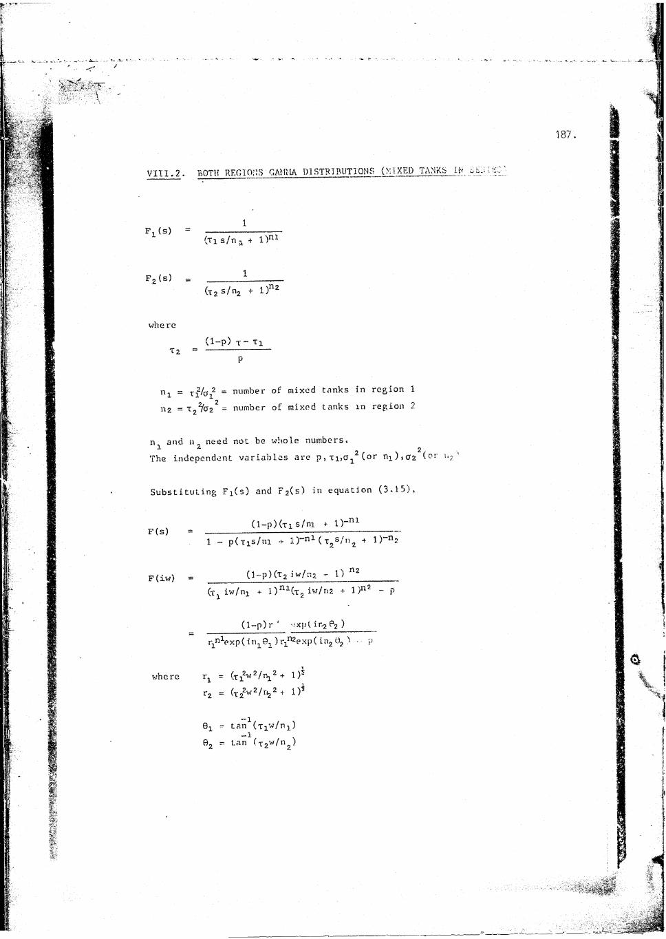
VIII.2. BOTH REGIONS GAHMA DISTRIBUTIONS (MIXED TANKS IN

1F,(s) = ----

(ti s/n j. + l)nl

F, (s)(x2 s/n2 + l)n2

wne re

Xz =(1 -p ) t - Ti

n i = tx/oj2 = number of mixed tanks in region 1 H2 = t„2/022 = number of mixed tanks in region 2

n and » need not be whole numbers.1 2 2The independent variables are n , (or n1)ia2 (or i.2 ’Substituting Fi(s) and F2(s) in equation (3.15)

F(s)(l-pXri s/ni + 1)'-ni

1 - p(Txs/nx + l)-nl( t2s/u2 + 1)-n.

F(iw) = (l-p)(T2iw/n2 - 1) nz

(t 1 iw/nj + l)ni(T2 iw/nz + 1)"'

(1-p) r exp(in2P2 )r1nlexp( in161) r1rtoexp( in2 8, 1 - ;>

where r1 = (r^w^/n 2 + 1 )s r2 - (t22w2/n2Z + 1)

- tan (Tiw/n2) -i02 - tan (tgw/n )

n2(1—p)r2 (cos n2 B2 + i sin 11282)

F ( iw ) — — ----— — — -------------------------------------------- _rxnir n2[c°s(niei + n^Gg) + i sinCn^G^ + n^Gz)] — P(l-p)r2n2(cos n202 + i sin n2e2)[r1n2r2n^:os(ni8i + n2©2)

- p - ir^Vg11in(niOx + n282)]____________ _r12n,r22ntos2(n19i + ngGg) - 2pr1n3 "(nx0i + n292)

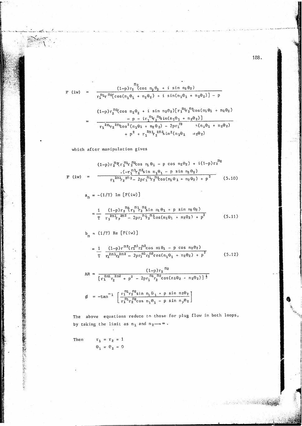
+ p2 + r 12n "1lr 22n^ in 2 ( n x© 1 =12© 2)which after manipulation gives

(l-p^jP^r l^os nx 8x - P cos n202) + i(l-p)r2. (-r-^-V^sin n. 9, - p sin n202)_______

F (iw) = ^ 2n ^ 2n 2_ 2 p r ^ 2 ^ o s ( n x 9 i + ngGg) + p 2 (5.10)

= -(1/T) Im [F(iw)]

1 (l-p)r2n^rxn r2n sin iixOx + P sin n2 82 )

T rx2n r22n2 - 2prxn ^2n ^os(nx8i + n202) + p2 (5.11)

b = (1/T) Re [F(iw)]n

1 (l-p)rn2(rinlr2n2cos ni8x - p cos 0202)

T rx2nlr22n2 - 2prxnlr2n2cos(n16 1 + 0282) + p (5 .12)

AR - a -p)r2n2

[ r 2nlr2 + p2 - 2pr1 r2 cos(ni92 "202)] -

r ^ r / ^ s i n n% 0 % + p sin n 29 2 |0 = -tan 1rxnir2n2cos n.9, - p sin n ?e 2 J

The above equations reduce to those for plug flow in both loops,

by taking the limit as n x and n 2— * “> .

189.

lim ni©!n1-»- oo

_ lim tan (ti w/ni) ri->- oo l/niwri (by application of L'Hospital's rule)

Similarly5 = wxs

Further useful special cases can be derived, e.g.

Instantaneous recycle;

Fjfs)

T2 = 0Therefore r% = 1 and 02 = 0

n

ni(l-p)ri sin ni0i

T [rini - 2pr1ncos m 8i + p2]

n1 (l-p)(r nlos n19I - p)T [r12rx- 2prinfcos n161 + p2 ]

Simple gamma distribution:

F l ( s )

T2 = 0, p = o

an = (l/T)r1n:Lsin bn = (l/T)r1nlcos ni&i

190.

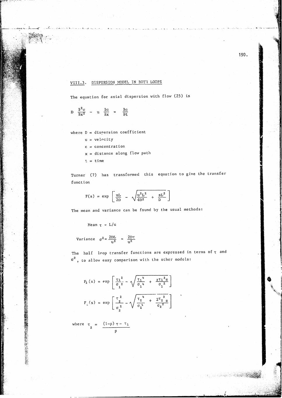
VIII.3. DISPERSION MODEL IN BOTH LOOPS

The equation for axial dispersion with flow (25) is

3^c 3c 3cD aP- - u 0 ' at

where D = dispersion coefficient u = velocity c = concentration x = distance along flow path t = time

Turner (7) has transformed this equation to give the transfer

function

F(s) = exp uL /u 2L2 . sL22D V 4D2 D

The mean and variance can be found by the usual methods:

Mean % = L/u

Variance = ^22u3 uz

The half loop transfer functions are expressed in terms of r and tf2 , to allow easy comparison with the other models:

?! (s) = exp T l a 2 T j 1* + 2 T 1 3S

V

F (s) = exp 2T 2 s

where x = (1-p) t -2 -------------

p

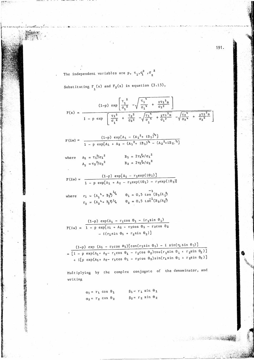
2The independent variables are p , »a2Substituting F (s) and F^Cs) in equation (3.15),

(1-p) expF(s)

2Tx3SPi2

1- p exp T1

°x2 I 2-P22 Tl 2 T 1 3 S A t2 1/ 0%4V 2X2 S

(1-p) exp[Ai - (Ai2+ iBi) ]F(iw) =

1 — p exp[Ax + A2 — (Ai2+ iBx)2, (2 +iB2.' ]

where Ax = Tx2/pi2 A, = T22/C22

Bx = 2tx^/ox2 B 2 = 2T2^/P22

F(iw) =(1-p) exp[Ax - rxexp(iBi)l

1 - p exp[Ax + A2 - rxexp(i6x) - r2exp(i02)]where rx - (A^(A/+ 0i = 0,5 tan (Bx/A^

r„ = (A%4+ &,2) \ @2 = O'5 tan^fBg/AgS

(1-p) exp(A1 - r^cos 0x ~ ir-j sin G^)F(iw) = 1 - P exp[Ax + A2 + rxcos 8x - r2Cos 6%

- i(rxsin 6 x + r2sin 0 2)]

(1-p) exp (Ax - rxcos Ai)[cos(nsin 6x) - i sln(rxsin 0x)]____= [1 - p exp(Ai4 A2- ricos - r2cos 82)cos(riSin 4 r2sin 82 )]

+ i[p exp(Ax+ Ag- ricos 8x - rgcos 82)sin(rxsin 6x + r%sin 8g)]

Multiplying by the complex conjugate of the denominator, and

writing

ax - rx cos ®x a 2 = r 2 cos 9 2

Gx= ?! sin @1Bg= r 2 sin 0 2

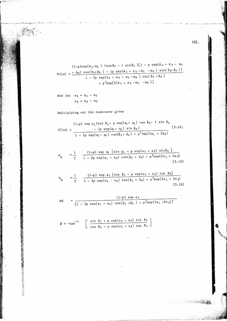
F(iw) =

(l-p)exp(Ai-Oi ) (cosBi - i sinPi )[l - P exp(Ai + A % - cti

- g2) cosQi+Gz ) - ip expCAi + Az -«i ) sin( gl+1 — 2p exp(Ax + A2 — otx ~ct2 ) cos(Bi +02 )+ p2exp[2(Ai + A2 -cti - otz ) 1

Now let ax = Ai - ax32 - A2 - Ct2

Multiplying out the numerator gives

(1-p) exp a-L (cos 0X- p exp(ax+ a2) cos 02- 1 sinF(iw) = ________ - ip exp (ax + a2 ) sin g2)__________________ (5.14)

1 - 2p exp (ax + a2 ) cos(@x+ 02 ) + p' exp(2ax + 2a2)

1 (1-p) exp ax Fsin Bi + P exp(ai + a2) sin0z 3____T 1 - 2p exp (ax + a2) cos(Bx + 02) •» p2exp(2ax + 2a2)

(5.15)

1 (1-p) exp ax [cos fix - P exp(ax + a2) cos 02]"7 1 _ 2p exp(ax : a2) cos(Gx + 02) + P*exp(2ai + 2a2)

(5.16)

(1-p) exp ax ________ __________[1 - 2p axp(ai + a%) cos(9x +62 ) + p 2exp(2ax +2az)]

n

AH

0 = -tan-x sin 0x + P oxp(ax + az) sin 02 cos 0x ~ P exp(ax + ag) cos 62

192.

193.

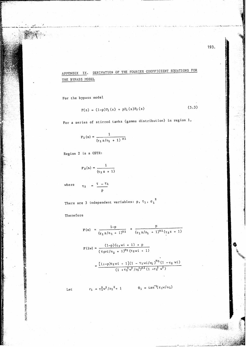
APPENDIX IX. DERIVATION OF THE FOURIER COEFFICIENT EQUATIONS FOR

THE BYPASS MODEL

For the bypass model

F(s) = (l-p)Fl(s) + pFi(s)Fz(s) (5'3)

For a series of stirred tanks (gamma distribution) m region 1,

Fi(s)(ris/ni +

Region 2 is a CSTR:

Fz(s) =(t 2 s + 1)

where %2 _ 'r ~ Tl

2There are 3 independent variables: p> Ti i 13x

Therefore

1-pF(s) =

F(iw)

+

Let

(Tis/ni + (ris/ni + l)"i(rzs + 1)(l-p)(T;Wi + 1) + P

( Tiwi /n^ + l)ni (tzwi + 1)[(l-p)t2wi + 1](1 - Tiwi/ni )n i d -T& wi)

( Y l T l ^ / n i T ' d +T2"

n = T%w*/ni*+ 1 @1 = tan-\Tiw/ni)

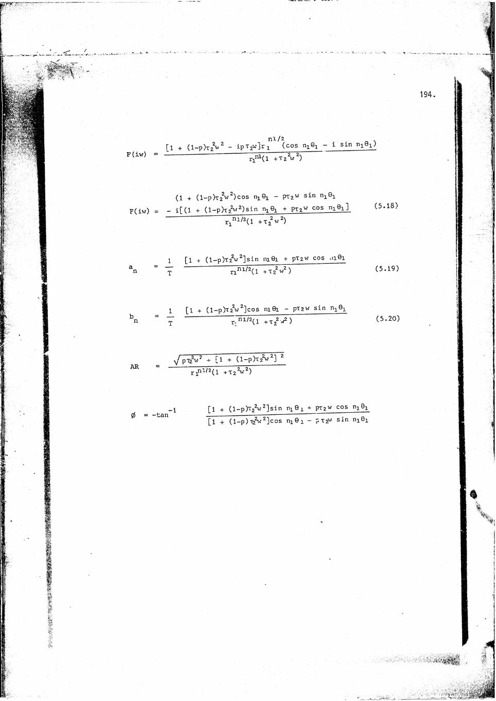
nl /2fl + (l-p)x22w2 - ipT2w]r! (cos ^ 0! - i sin ^ 81)

P<1W> " ----------- ri"Hl

(1 + (l“-p)xj w *)cos n^Gi - px2w sin n^Qi F(iw) = - i[ (1 + (l-p)T2 2)sin n^Gi + px2w cos nx8x]_

" "r1ni/2(l +T 5»2 w 2)

1 [1 + (l-p)T£2w 2]sin m 61 + pt2W cos .1101= T +T22w2] (5'19)

1 [1 + (l-p)T:22w 2]cos m9i - pTaw sin ni@i" Y 1. (5-20)

pT22W ? + [ l + (l-p)T^2]

0 = -tan_1 [1 + (l-p)T22w 23sin % 8 1 + pr2w cos ni9i

[1 + (l-p)'a2w 2]cos nz 9 1 - p t 2w sin ni8i

APPENDIX X . SIGNIFICANCE OF THE SHAPE OF THE AMPLITUDE RATIO PLOT

OF THE LONG REACTOR

The amplitude ratio and phase lag plots of the long vessel (appen­dix 4) all have a similar characteristic shape, with a hump at about n=15 (the natural frequency). In some cases, further maxima at higher frequencies (harmonics) can be discerned. Typical plots are reproduced below.

noiselog AR

- 2

2ww. nnfrequency, w

00n

wnfrequency, w

FIGURE X . l . SHAPE OF EXPERIMENTAL AR AND 0 PLOTS OF

THE LONG VESSEL

The most satisfactory explanation for the occurence of peaks in the AR plot is recycling of material in the reactor. This also accounts for the oscillatory nature of the RTD curve. In order to investigate the significance of these peaks, we shall study the AR and 0 plots of the "recycle model" developed in section 5.

We first investigate the shape of these curves for the case of plug flow in both loops of the recycle mod”'..

,/IX

log AR

2%w nfrequency, w

0 -;

0

nfrequency, w

FIGURE X.2. SHAPE OF AR AND 0 PLOTS OF THE RECYCLE MODEL WITH PLUG FLOW IN BOTH LOOPS .

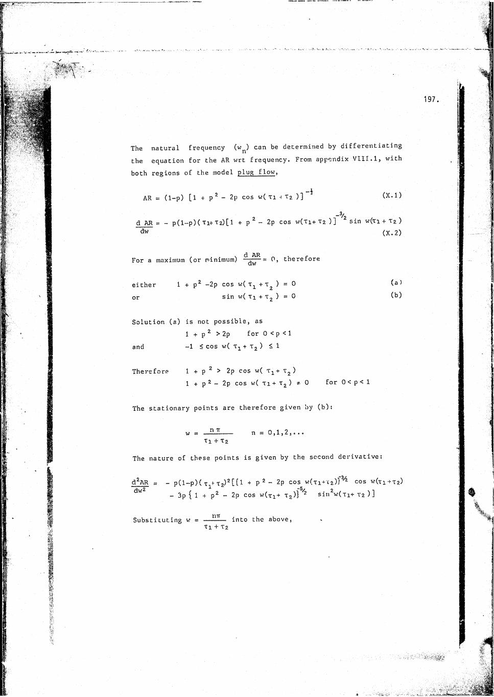
The natural frequency (w ) can be determined by differentiating the equation for the AR wrt frequency. From appendix VIII.1, with both regions of the model plug flow,

AR = (1-p) [1 + p 2 - 2p cos w( Ti -i t2 )] ' (X.l)

a AR = - p(l-p)( Ti+ t2)[ 1 + p 2 - 2p cos w(Ti+ T2 )] sin w(ti + t2 )dw (X.2)

For a maximum (or minimum) therefore

either 1 + p2 -2p cos w( + t ) = 0 (a5or sin w( Ti + t2 ) =0 (b)

Solution (a) is not possible, as1 + p 2 > 2p for 0 < p < 1

and -1 < cos w( t-l + t2 ) <1Therefore 1 + p 2 > 2p cos w( T%+ T2 )1 + p 2 - 2p cos w( T1 + X2 ) f 0 for 0 < p < 1The stationary points are therefore given by (b):

w = — n = 0,1,2,...Ti + t2

The nature of these points is given by the second derivative:

d2rn = - p(l-p)( T I-t2)2[{1 + P 2 - 2p cos w(ti+'i2))~3/2 cos w(t]dw2 _3p { 1 + p2 - 2p cos w(Tl+ t2)} 2 sin w(xi+ ta )]

Substituting w = — — — into the above, T l + T 2

(. p(l-p)(T2-T2)*(l + + 2p)d^AR I - p(l-p)(Tl+ T2):(l + P* - 2p)~^ for n even

-3/rrfl-nK T-ri- t n ) 2 (i + d 2 + 2p) 2 for n odd

f - pCtx •»• t2) 2< 0 for n even

= <p(l-p)(T1+ T2) 2

(1+P): " °> o for n odd

Therefore maxima occur at w = hti /(ti+t 2) with n - 0.2,6...and minima occur at w - nir/(t i+t 2) with n = 1,3,5... (X.4)

Fron; equation (X. 1) : AH (max) = 1, AR(min) = (1-p) /(t+p)

The natural frequency is thus w - 2ir/(t i +t 2) (the first peak inthe AR plot) and further peaks are harmonics of the natural fre­

quency.

Furthermore, the phase angle at the natural frequency is given by

0 = -tan -1 r sin wn Ti 4- p sin wpron cos - P cos W 2 J

tan 1 sin T __________________________9 t r T l

cos 2'if't i _ p cos (2 tr - 2ttti )

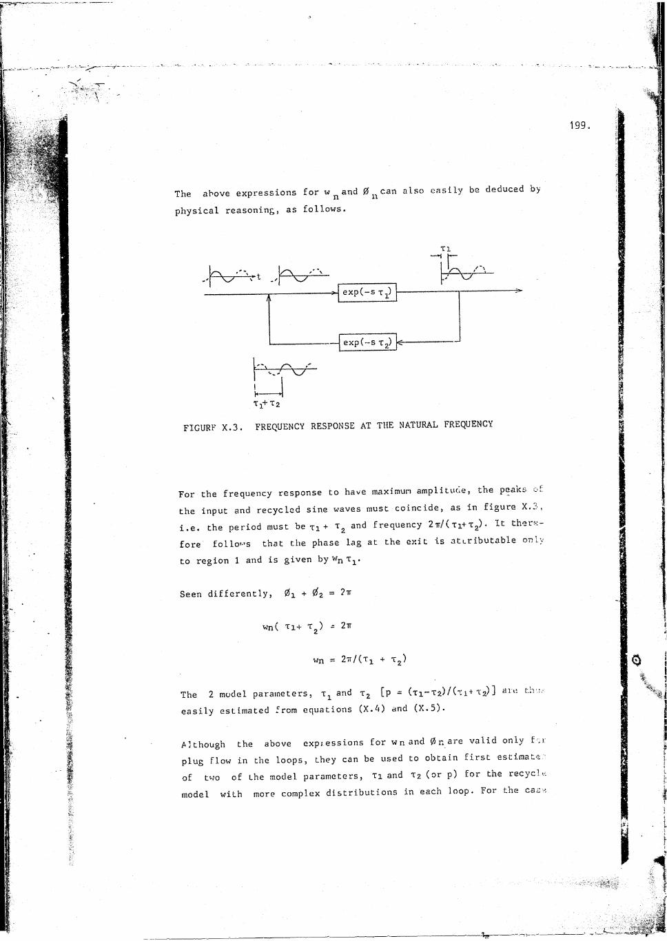
The above expressions for tv n and 0 n can also easily be deduced by physical reasoning, as follows.

T 1

exp(--s t 2)

exp(-s T j)

H 4T]+T2

FIGUEF X.3. FREQUENCY RESPONSE AT THE NATURAL FREQUENCY

For the frequency response to have maximum amplitude, the peaks ot the input and recycled sine waves must coincide, as in figure X,..', i.e. the period must be Ti+ Tg and frequency Zir/CTi+Tg). Chere-fore follows that the phase lag at the exit is attributable only to region 1 and is given by wnSeen differently, 0x + $2 =

wn( 11+ Tg) = 2irwn = 2 tt/( t 1 + t 2 )

The 2 model parameters, t1 and t2 [p = (ti-Tg)/(T1+ tg) ] are f.h :; easily estimated from equations (X.4) and (X.5).

A 1 though the above expressions for w n and 0 n are valid only for plug flow in the loops, they can be used to obtain first estimau^ of two of the model parameters, Ti and Tg (or p) for the recycle model with more complex distributions in each loop. For the cat,-:

of a tanks—in—series model (gamma distribution) in each loop, thephase angle at the natural frequency is also only dependent onregion 1 and is given by

0n = — n i tan (wnT]_/n i)w n is found from

nxtan1(wnT1/n i) + n 2tarr1(wnT2/n 2) -

For large n

tan1 (w^Ti/nx) a Wn^/ni

and similarly for n %

Then the expressions for 0 n and w n become

0n s - wn tiw n s 2 ir/ ( t t 2)

The more well-mixed are the regions in the two loops of the recycle model, the less well-defined are the peaks in the AR plot and the more the phase lag plot approaches a straight line.

APPENDIX XI. COMPUTER PROGRAMS

XI. 1: Program for taking RTD readings.XI.2: Program for averaging a number of RTD curves.

XI.3: Program for normalisation, exponential tail fitting and

plotting of RTD curves.XI.4: Program for calculating Fourier coefficients , amplitude

ratio, phase lag and the Fourier series tor the experi-

mental curve.

Programs for least-squares fitting of mafaamatical models to the experimental Fourier coefficients, producing the model parameters:

XI.5; Recycle model with gamma distributions

XI.6: Recycle model with axial dispersion in

XI.7: "Bypass model"

Programs for calculating model parameters as functions of fre­

quency:

XI.8: Recycle model with gamma distributions in both loops.

(Q-MIX (XI.8) is a modification of P-MIX (XI.5). The programs of appendices XI.6 and XI.7 can similarly be modified fox calculating parameters as functions of frequency).

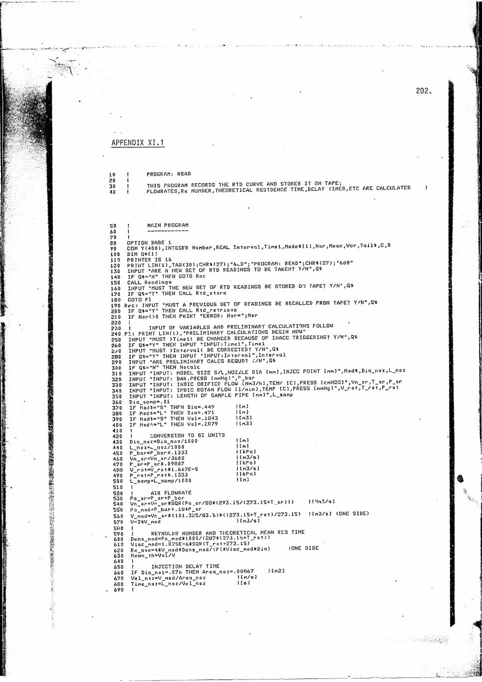
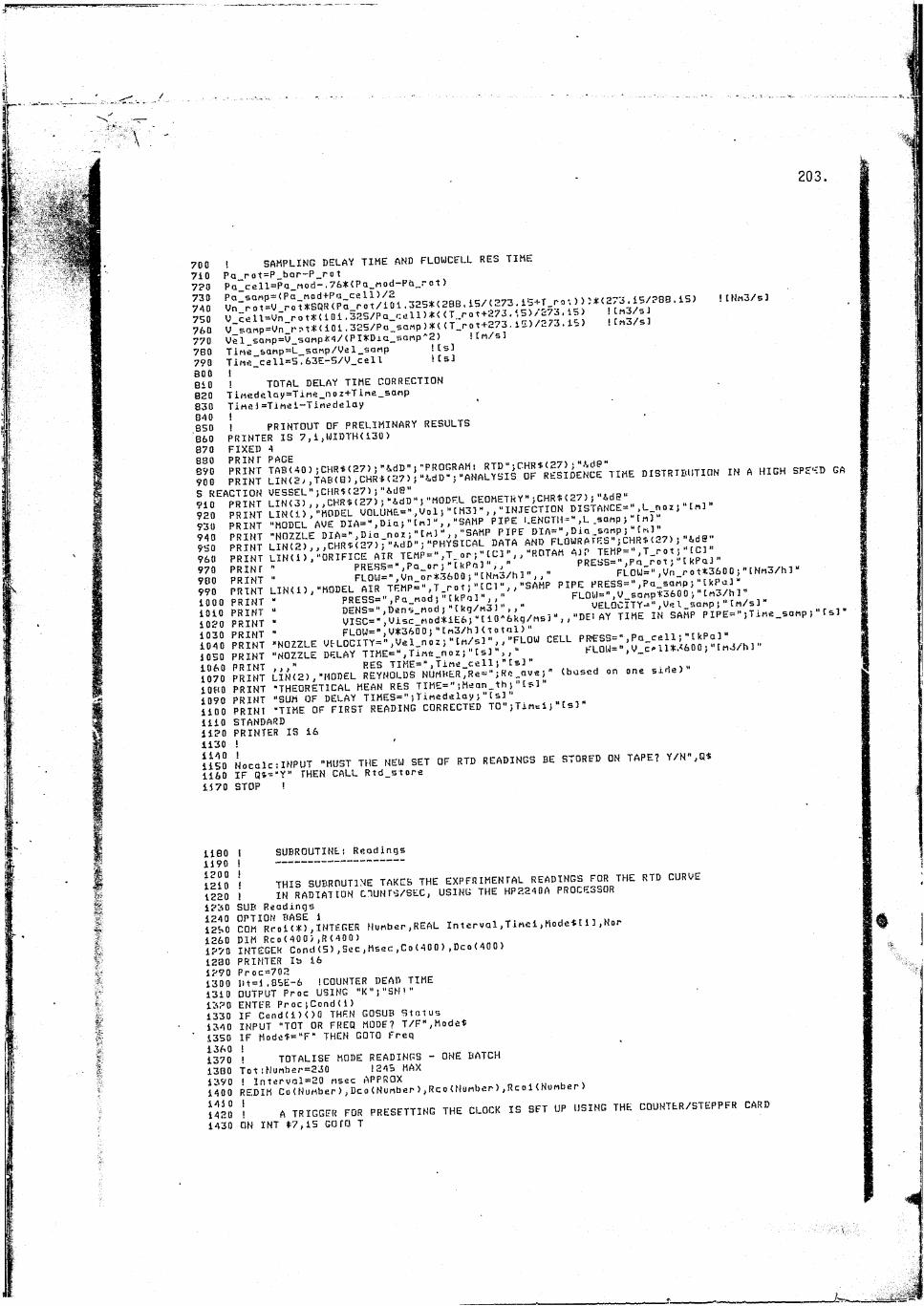
APPENDIX X I . 1

10 ! PROGRAM: READ

E I « E cau=ul»tE»

5060708090100150120130140ISO160170180

! MAIN PROGRAM

IC O M ^YM OO) ,INTEGER Number,REAL Interval,TlMel,Mode$[1],Nor,Mean,Vor,Ta11$,C,BDIM Q$tl3PRINT^LIN(i),TAB(30);CHR$(27>) "PROGRAM: READ“jCHR$(27)j"6de"INPUT "ARE A NEW SET OF RTD READINGS TO BE TAKEN? Y/N",Q$IF Q$=“N" THEN GOTO RecINPUT "MUST9THE NEW SET OF RTD READINGS BE STORED O'! TAPE? Y/N",R$IF Q5="Y“ ‘ " J ^GOTO PI

THEN CALL Rtd_storeL90 R e c : INPUT "MUST A PREVIOUS SET OF READINGS BE RECALLED FROM TAPE? Y/N",Q$20 0 210 220 230 240 250 260 270 280 290 300 35 0 320 330 340 35 0 360 370 380 390 400 450 420 430 440 450 460 470 480 490 500 510 520 530 540 550 560 570 580 590 600 610 620 630 640 650 660 670 680

IF Q$="Y" THEN CALL Rtd„retrieve IF N o r O O THEN PRINT "ERROR: Nor = "}NorII

PI lINPUT OF VARIABLES AND PRELIMINARY CALCULATIONS FOLLOW

j, : PRINT LINCi) , "PRELIMINARY CALCULATIONS BEGIN NOW"INPUT "MUST >Timel< BE CHANGED BECAUSE OF INACC TRIGGERING? Y/N",0$IF Q$="Y" THEN INPUT "INPUT : T-tnel ", Tinel INPUT "MUST IlntervaK BE CORRECTED? Y/N",Q$IF Q5="Y" THEN INPUT "INPUT:Interval",Interval INPUT "ARE PRELIMINARY CALCS REQUD? i'/N",Q$INPUT "INPUT: MODEL SIZE S/L,NOZZLE DIA [mnl,INJEC POINT C m ! “,Mod$,Dia_noz,L_noz

BAR.PRESS CnmHgl “,t>_barINDIC ORIFICE FLOW CN«3/hl,TEMP EC1,PRESS CcmH201",Vn_or,T_or,P_or INDIC ROTAM FLOW E1/nin3,TEMP EC],PRESS [mmHq]",V_rot,T_rot,P_rot LENGTH OF SAMPLE PIPE Emm]",L_samp

INPUTINPUTINPUTINPUT

"INPUT:"INPUT:"INPUT:"INPUT:

Dia sortp=.01 IF Ma.1$="S" THEN Did".449

THEN Dia=.471 THEN Vol=.lB43 THEN Vol=.2879

IF Mod$="L"IF Mod$*"Sr IF Mod'l'="L"!! CONVERSION TO S3Dla_noJ!=Dia_n(iz/10 0 0 L_noz=t._noz/10 0 0 P_har=P_bar.F.i333 Vn ar=Vn or/3600 P_or=P_or*.09807 V_rot=V_rot*l.667E-5 P_rot=P_rot*,1333 L_sampBL_saMp/l0 00

UNITS

! Cm3 ! Cnl ! Cm33 I Em3]

! Cm ]! Chi I CkPa]!Cm3/s3 ! EkPa)!Cm3/s ] IEkPa]I Em !

! AIR FLOWRATEPa_or=P_or+P_bar Vn_or=Vn_or*SQR(Pa or/B8*(293.15/(273 .15+T..or )) >Pa nodi«P„bar+.18kP_orV_Mod=Vn_.or*<101,325/03.5>*< <273,15+T_rot>/273.15) V=2W_nod ! Em J/b )! REYNOLDS NUMBER AND THEORETICAL MEAN RES TIMEDens fiod=Pa Mod*l 0 0 0/(287*< 273 .15+T _r o t ) )Visc""nod = l. 075E-6*SQR (T_r ot+273 .15)Re_ave=4*V_Mod*Dens_Mod/xPI)KVIsc_nodYDla) I ONE SIDEMean th=Vol/V I! INJECTION DELAY TIMEIF Dia_noz= , 076 THEN Area,.noz=. 00867 Vel_noz=V_Mod/Area_noz I Cm /s ]Tine noz=L n oz/VeInez ICsJ

1ENm 3/s ]

! Cm 3/5] (ONE SIDE)

! Cm23

203.

700 ! SAMPLING DELAY TIME AND FLOWCELL RES TIME710 Po_rot=P_bar-P-rot7?0 Pawcell=Pa M0d-,76^CPQ„M0d-F,a-rat)

I B s S S = ; E i E E i r i E r770 Vel saMp=V__sanpf4/(PI^Dia_samp 2) ! LM/s780 TiMe_sanp=L_saMp/Vel_saMp !tsl790 TlMe_cell=S.63E-5/V_cel1 .CsJBiO i TOTAL DELAY TIME CORRECTION820 Tinedelay=Tlrte_noz+Ti*e_sanp 830 Tinej=TiMei-TiMedelayQ5B i PRINTOUT OF PRELIMINARY RESULTS860 PRINTER IS 7,i,UIDTH(130)870 FIXED 4

?H EE -»«"im s'e™ m

!E EE s :^ s s - a a s T S S K - . * <-*»- - •i->- -

1080 PRINT "THEORETICAL MEAN RES TIME=";Meon_th> tsls ' - . r w , -

1110 STANDARD 1120 PRINTER IS 16 1130 !tisS Lcalc,INPUT "MUST THF NEW SET OF RTD READINGS BE STORED ON TAPE? Y/N",Q$1160 IF q$="Y" THEN CALL Rtd_t.tore ii 70 STOP !

1180 I SUBROUTINE I Readings

!ui! RT1CURVE1230 SUB Readings12S0 CO^RroiC^f, INTEGER Hunber.REAL In ter val .Tihel, Modet 113 , Non 1260 DIM Rco(400) ,R(400) ,.nn,1270 INTEGER Cond(5),Sec,Msec,Co(400),Deo<400)1280 PRINTER lb 16 1290 Proc=7021300 !>t=l,B5E~6 !COUNTER DEAD TIME1310 OUTPUT Proc USING "K “ ; "8N ! "1320 ENTER Proc}Cond(i>1330 IF C o n d d ) < >0 THEN GOSUB Status 1340 INPUT "TOT OR FREQ MODE? T/F",Mode$1350 IF Made$="F" THEN GOTO Freq1370 ! TOTALISE MODE READINGS - ONE BATCH1380 Tot iNu tber=230 !243 MAX

i A TRIGGEI. FOR PRESETTING THE CLOCK IS SET OP USING THE COUNTER/STEPPFR CORO1430 ON INT *7,15 GOTO T

\ ; -

203.

700 ! SAMPLING DELAY TIME AND FLOWCELL RES TIME710 Pa_rot=P_bar-P_rot7?0 Pa cell=Pa nod-.76*(Pa_ttod-Pa_rot}

I770 Ve 1 scmp=V_saMp#4/(PI*Dia_saMp 2) !Efi. s3 780 TiMe_sanp=L_sanp/Vel_saMp Us)790 Tlfie_celI=S. 63E-5/V_cell .is)B<0 ! TOTAL DELAY TIME CORRECTION820 TlHedeIay=TiMe_noz+Tlne_sonp 830 Tine)=TiMei-Tittedelay350 ! PRINTOUT OF PRELIMINARY RESULTS860 PRINTER IS 7,1,WIDTH(130)870 FIXED 4

E E E i «»,=« ^ =»

# * # k .

: ^ K K : R T R : - ] ; ! ; y . r (bas«d.n, ,id«).iOflO PRINT "THEORETICAL MEAN RES TTME=" ;Mean_ths (s): : : : ^ F % ; T i : a ' ^ a ^ i T i m e i r c : -1110 STANDARD 1120 PRINTER IS 16 1130 !1150 Nocalc U NPUT "MUST THE NEW SET OF RTD READINGS BE STORED ON TAPE? Y/N",Q$1160 IF Qt-'Y" THEN CALL Rtd_stope 15 70 STOP !

1180 1190 1200 1210 1220 1230 1240 12S0 1260 1270 1280 1290 1300 1310 1320 1330 1340 1350 1360 1370 1380 1390 1400 143 0 1420 1430

SUBROUTINE: Readings

I RT“ CURVESUB ReadingsCOM^Rnol(*),INTEGER Number,REAL Inierval,Timel,ModetC11,Nor DIM Rco(400),R(400 )INTEGER Cond(5),Sec,Msec,Co(400),Deo(400)PRINTER lb 16 Proc=702l)t = l.85E-6 I COUNTER DEAD TIME OUTPUT Proc USING "K"s"SN>”ENTER ProcjCond(1)IF Cond(l)()0 THEN GOSUB Status INPUT "TOT OR FREQ MODE? T/F",Modet IF HodeT="F" THEN GOTO Freqi TOTALISE MODE READINGS - ONE BATCHTot:HuMber=230 I 245 MAX! Interval=20 msec APPROXREDIM Co(HuMber),Dco(Nunber>,Rco(NuMber),Rcol(NuMber>l A TRIGGER FOR PRESETTING THE CLOCK IS SET UP USING THE COUNTER/STEPPFR CARDON INT *7,15 GOrO T

204.

1440 1450 1460 1470 1480 1490 1500 151 0 1520 1530 1540 1550 1560 1570 1560 1590 1600 161 0 1620 1630 1640 1650 1660 1670 1680 1690 1700 1710 1720 17.30 1740 1750 1760 1770 1780 1790 1600 1810 1820 1830 1840 1850 1860 1870 1880 1890 190 0 1910 1920 1930 1940 1950 i960 1970 i960 1990 2000 2010 2020 2030 2040 2050 2060 2070 2080 2090 2100 2110 2120 2130 2140

' 2150 2160 2170 2180 2190 2200 2210 2220 2230 2240

CONTROL MASK 7)128 CARD ENABLE 7OUTPUT Proc USING "K";"SN;SM,0,1}ST,1,1,1»1!ENTER ProcjCond(2)IF Cond < 2) < >0 THEN GOSUB Status.PRINT “SYSTEM READY FOR TRIGGER”CRT OFF W !GOTO tiW T P m ^ B F H S NOFORMATrTP.0,0)ST,l,2,l,0,RP,230,WN,18;R,:,l,2,llNX)TE!"ENTER 702)Cond(3>,Cof*),SfiC,Msec CRT ONPRINT "TRIGGER ACTIVATED”PRINT "READINGS COMPLETE"IF C o n d < 3)< > 0 THF N GO S U B Status Elap t ina-Sac+Msec/1000 !S E C O N D S I n t erval= 2 lap_ tIne/Nunber !secDco(l)=Co;i)Rco(i)=Dco( D/Interval Rcol(l)=Rco(i)/ti-Dt*R<:o(lFOR 1=2 TO Number ^IF C o d ) <0 THEN Co (I >=00 (I) +32768

Dcoa)=Cod)-Co(I-l)IF D c o d X O THEN Deo (I )-Deo d )+32768R w l ( n % d ( / d - D t * R c , d ) ) ICORRECTION FOR DEAD TIME

Tine 1=1nterval/2 t ESTIMATEGOTO Pr1 FREQUENCY MODE RFADINGS - ONE BATCHFreq iNunber=392 ! GATE TIME =10nsec ! Interoal=12nsec APPROXREDIM DcotNunber),Rco(Number),Rcoi(Number)| A TRIGGER FOR PRESETTING THE CLOCK IS SET UP USING THE COUNIER/STEPPFR CARDON INT *7,15 GOTO 5 CONTROL MASK 7;128 CARD ENABLE 7OUTPUT Proc USING "K"t"SN;SM,0,1;ST,1,1,1,1!"ENTER Pr ocjCond <4)IF Cond<4)< >0 THFN GOSUB Status PRINT "SYSTEM READY FOR TRIGGER"CRT OFF VsGOTO VOUT PUT 702^BFHS NOFORMATi “T P ,0,0 ;SP,i ,4 ,1 jRP,3 9 2 }UN,11 }RC,1 ,4 ,1 jNX ;TE ! "ENTER 702jCond(5),Dco<*>,Sec,Msec CRT ONPRINT "TRIGGER ACTIVATED”PRINT "READINGS COMPLETE"IF Cond<5)00 THFN GOSUB Status Elapwt tMe=Sec+Msec/l000 I sec Interual=Elap_t ine/Nunber !secFOR 1=1 TO Number

Rr o <I)=Dc o <I)/.01Rc ol (I)=Rco<I)/d-Dt*Rcod))T imel“In tfirual- 0 06 !ESTIMATE

-IS f, CRT PBIIITOUI Of TIE C O R R E C T E D C - R O T T S REO UIRtDT Y/K",0«IF Q$="N" THEN SUBEXIT M=INT(Nunber/lf>-,001) + l FIXED 0 MAT R=Rcoi REDIM R(IOYM)PRINT LIN(2)FOR 1=1 TO M

PRINT LINCO)FOR K=0 TO 9

PRINT USING J.m3) R (K#M+I >Im3 1 IMAGE *,MDDDDDD,iX

NFXT K NEXT C STANDARD

22S0 2260 2270 2280 2290 2300 23 j 0 2320 2330 2340 23 0 2360 2370 2380

SUBEXIT| PROCESSOR STATUS READ, IN CASE OF ERRORStatus, OUTPUT Proc USING "l<”)"ST2"ENTER Proc;Stat*

I S i S S H I B S E SPRINT “EXTENDED STATUS IS,")Sta1$RETURN SUBEND '

CondS"CondS*

2390 2400 2410 2420 2430 244 0 2450 2460 2470 2400 24 90 2500 2510 2520 2530 2540 2550 2560 2570 2500 2590 260 0 261 0 2620

SUBROUTINE: Rtd_store

", THIS SUBROUTINE STORES THE RTD CURVE ON TAPESUB Rtd_storeCOM'Rc.un^*),INTEGER Number,PEAL I n t e r v a l , TlMel,Mode$[lI,Nor,Mean,Var,Tall«,

INPUT^OPTIONAL TRUNCATION OF NUMBER OF READINGS; INPUT N (or 0)",NIF N< >0 THEN Nu m1)--=N REDIM Rcount(NuMber)DISP “INSERT THE DATA STORAGE CASSETTEINPUT "Mi‘ST EXISTING FILES BE DISPLAYED? Y/N",02$INPUT “ENTER THE FILENAME FOR THE CURRENT DATA",FIle$Bytes=8>K(NuMber P7)Rec=INT(Bytes/256)+i CREATE Fl :e$,RecPRINT tijHode$,Nufib«r,Interval,TiM«l,Rcount(*),NorIF (Nor-1) OR (Nor-2) THEN PRINT *l;Mean,VarIF Tail$=*Y" THEN PRINT tl{C,B AUBEND !

2630 2640 2650 2660 2670 2600 2690 2700 271 0 2720 2730 274 0 2750 2760 2770 2780 2790 2800 2810 2820 2830 284 0 2850 2860 2870 2880 2890 2900 2910 292 0 2930 294 0 2950

1 SUBROUTINE: °td_retrieve

!, t h i s SUBROUTINE RETRIEVES A PREVIOUS RTD CURVE FROM TAPESUB Rtd..retrieve2'3T.unU*),INTEGER Nunber.REAL Interval,TMel,Mode$[iI,Nor,Mean,Var,Tail*DIM FUe$[6JDISP “INSERT THE DATA CASSETTE"INPUT "MUST EXISTING FILES BE DISPLAYED? Y/N",Q1$IF qi$=“Y “ THEM CAT „ „ „INPUT "ENTER THE FILENAME TO BE RETRIEVED ,FiletASSIGN *1 TO FiletREAD $1,1 t ,READ ti jMode$,Nufiber,Interval,TIMe 1 REDIM Rcotint(Nunber5 READ *LiRcount<*),NorK p r ^ O E S ^ I S ' ^ V F ^ r ^ ' E ^ ^ T ^ r T A I L ? Y/N",Tail$P R I N ^ L I N U ) , F U e $ ; ^ H A S ^ P E N RETRIEVED" ;SPA(S)rMODE ISPRINT USING Im I : T IfieiPRINT "NUMBER-"jNuMber(SPA(S)JIFIT L l $ = h"Y”ITHFNnpRINT1 “EXP TAIL: Y-C.EXP(-Bt) C="jCi" B="; B IF Nor-1 THEN PRINT USING Im3)Mean,Var IF Nor-2 THEN PRINT USING Im 4 jMeon.Var ImI:IMAGE "FIRST READING AT",M .DDDDOD

E ESUBEND I

';Mode$

205.

C,B

t secA2I"[DIMLESS)"

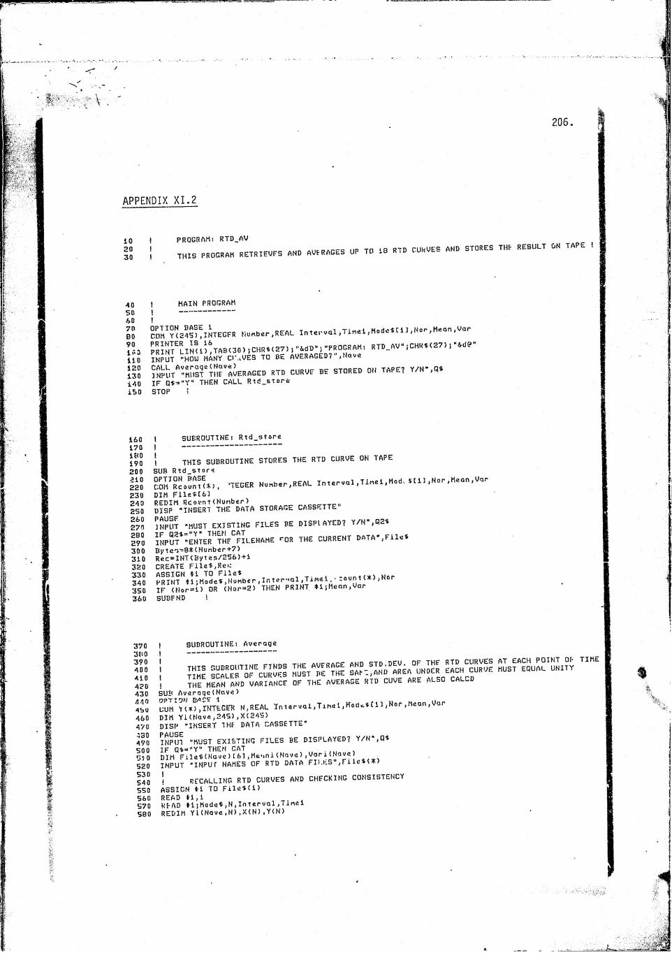
APPENDIX XI.2

102030

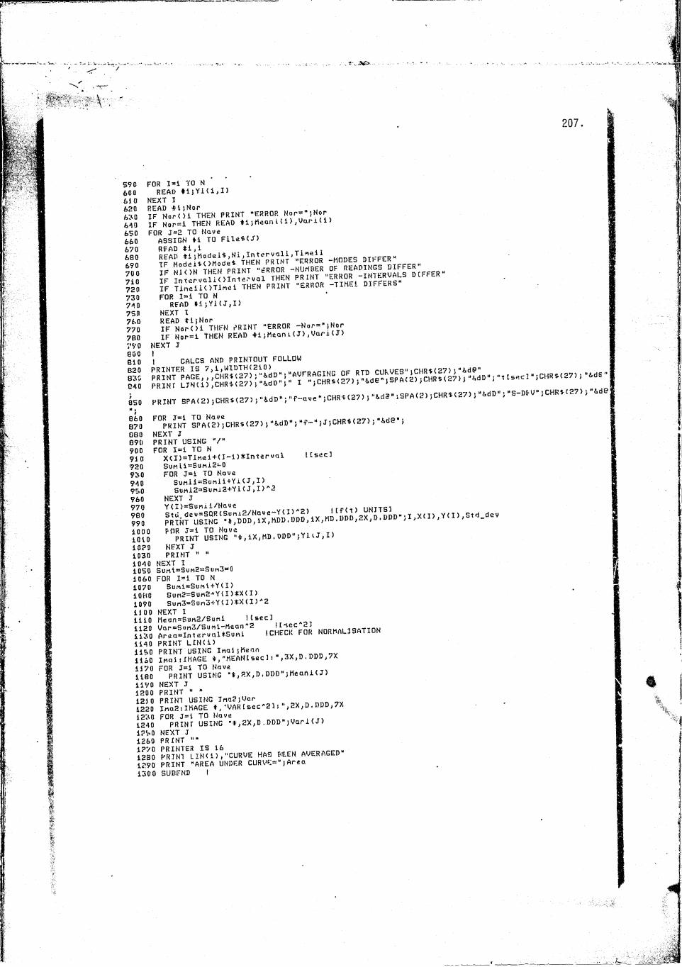
PROGRAM: RTD_AVTHIS PROCRSH RETRIEVFS AND AVERAGES UP TG IS RTD CURVES AMD STORES THE RESULT ON TAPE .

40 ! MAIN PROGRAM

60 !M COMTzSsWNTEGFR Kunber.REAL Interval,TiM«l,M.d«$ri],N.r,Me.n,VarE;51! ^HPUT^"MUST6THE^AVERAGED RTD CURVE BE STORED OH TAPE, Y/»-,0.140 IF Q$-”Y" THEN CALL Rtd_store ISO STOP 5

160 1 SUBROUTINE: Rtd_store170 ! ------------------------i?S I THIS SUBROUTINE STORES THE RTD CURVE ON TAPE200 SUB Rtd_store15! -TEGER Nurtber ,REAL , „ „ r ,.1 ,Tl„,l,«-d. , , H „«,r , V,b230 DIM FileSttilgs! M S p " ' I N S E R l % ' ' D A f A STORAGE CASSETTE"27% "MUST EXISTING FILES BE DISPLAYED? Y/N",Q2*270 INPUT^ENTER^THF^FILENAME rOR THE CURRENT DATA",File*300 By tc3"=S$(Number+7)310 Rec*>INT<Bytes/2S6) + i 320 CREATE File*,Re-:

360 SUBFND !

370 i SUBROUTINE: Average

I i S=ii?;H=S5;"EF"“430 SUB Averoqc(Nave)4SU GUM YuT!INTEGER N.REAL I n t e r v a l , Tinel,Mod.*Cl3,Nor,Mean,Vor 460 DIM Yi<Nave,245),X<245)470 DISP “INSERT THP DATA CASSETTE"490 INPUT “MUST EXISTING FILES BE DISPLAYED? Y/N",Q$S00 IF Qt="Y" THEN CAT , N

540 ! RECALLING RTD CURVES AND CHECKING CONSISTENCY550 ASSIGN *i TO FileKl)560 READ frl,l , «570 READ *l;Mode$,N,Interval,iinel 580 REDIM YKNavc ,N> ,X(N> ,Y(N)

590 600 65 0 620 630 640 650 660 670 680 690 700 710 720 730 740 750 760 770 780 790 800 810 820 830 040850

FOR 1=1 TO NREAD *1jYi(1jI)

NEXT IIFANor<)i°THEN PRINT "ERROR Nor=";Nor IF Nor=i THEN READ *1; Mean t (1), V a n (1)FOR J=2 TO Nave

ASSIGN *1 TO FileS<T)READ *1,1 ,, t i — ^ i

llllillillls-'-FOR 1=1 TO N

READ *1}Y1(J,I)NEXT II F ^ o r O l ^ T H E N PRINT "ERROR -Nor=",NorIF Nor=l THEN READ *1)Meani(J),V a n <J )

NEXT J1 CALCS AND PRINTOUT FOLLOW

PRINT S P A < 2 ) ; C H R $ < 2 7 > ;,i4.dD";"f-aveN;CHR-i<27>) " 6 d 3 " $ S P A ( 2 ) ; C H R $ ( 2 7 ) “6dD";"S-DPV"jCHRS<27)

860 870 080 89(1 900 910 920 930 940 950 960 970 980 990 1000 1010 1020 1030 104 0 1050 1060 1070 10H0 1090 1500 1110 1120 1130 1140 1150 1160 1170 1180 1190 1200 125 0 1220 1230 1240 1250 1260 1270 1280 12.90 130 0

!(sec]

F°PRINT SPA(2) jCHR«<27) ) "6dDn5 "f-** }J fCHR*<27) j "6de" j NEXT JPRINT USING “/"FOR 1=1 TO NXa)=Ti«ei + <I-i Interval

S u m (1=SUM12-0 FOR J=i TO Nave

Sun!i=Sunli+Yi(J,I)SuMi2=SuMi2+Y i(J ,I)A2

NEXT J

FOR u=i TO Nave . _PRINT USING ,IX,HD.ODD"}Yi[J,I)

NEXT J PRINT " "

NEXT I , „S u m 1=Su m2=Sum3=0 FOR 1=1 TO N

Su m 1=Su m I+Y(I>Bum2=Sum2j' Yd) X (I)Su m 3=Su m 3+Y(I) ( 1 5 A2

NEXT I ,r ,Mean=Surt2/Suni ![sec]

. c H ^ r F O R NORMALISATIONPRINT LIN(i)PRINT USING InaliMeanImo11IMAGE *, "MEAN!seeli“,3X,D .DDD,7X FOR 1=1 TO Nave

PRINT USING 2.X,D. DDD"}Meani<J)NEXT J PRINT " »^ l S % / a Z c " 2 i r , 2 X , D . D D D , 7 XFOR J=t TO Have

PRINT USING "t,2X,D.DDD")VarI<J)NEXT J PRINT ""PRINl^LINd) , "CURVE HAS BEEN AVERAGED"PRINT "AREA UNDER CURVE"")Area SUBFND I

208.

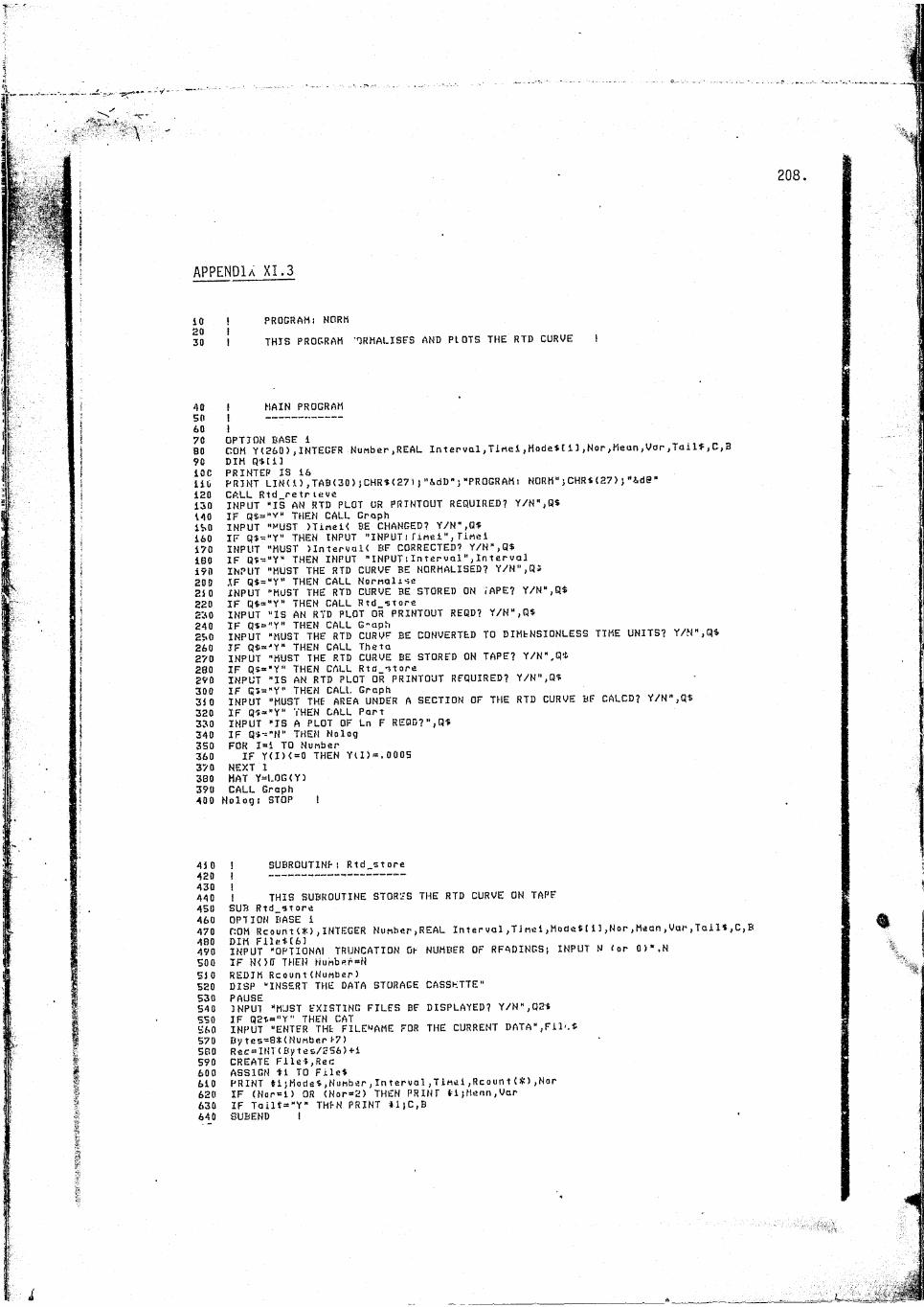
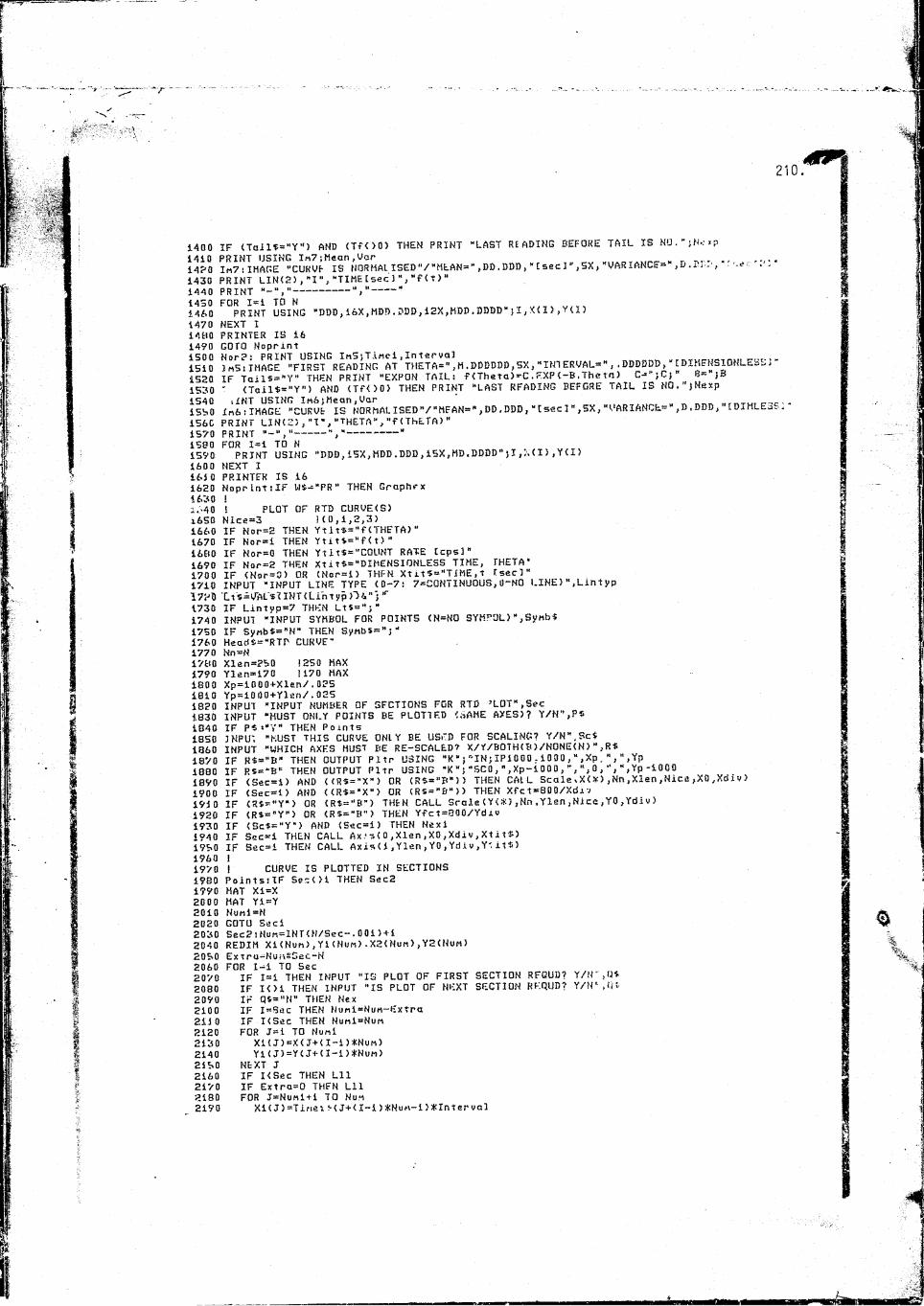
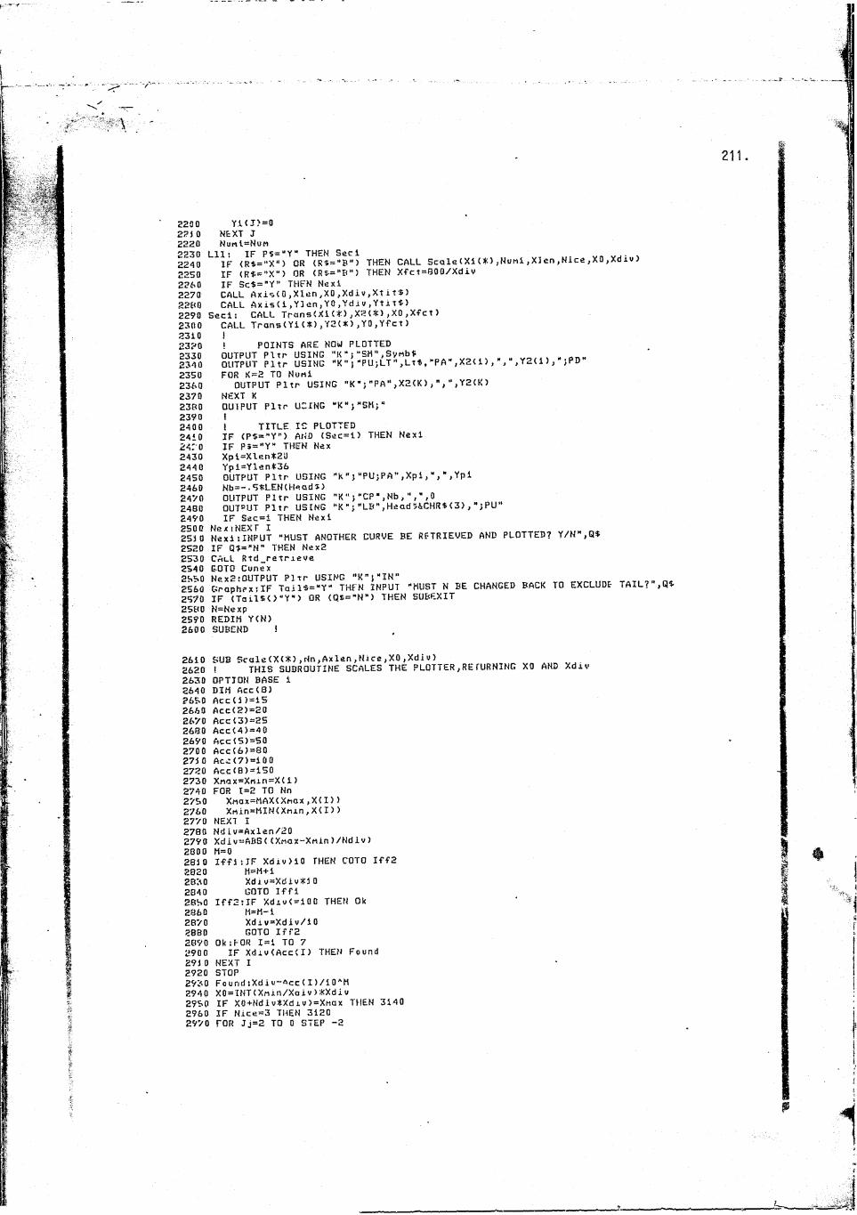
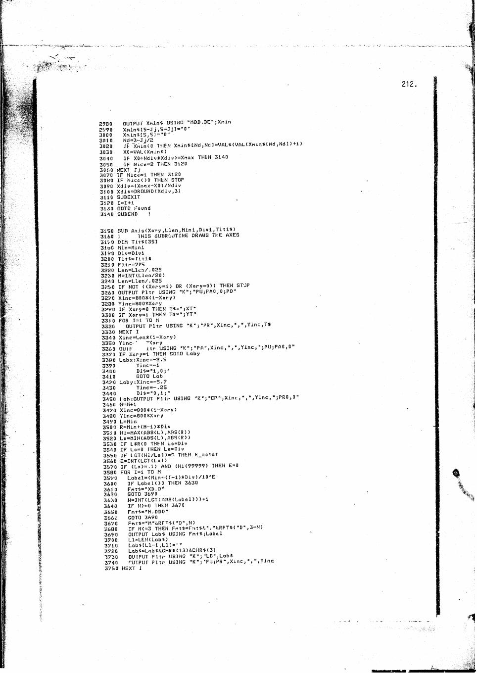
APPENDIa X I . 3

10 ! PROGRAM: NORM20 !30 ! THIS PROGRAM '1RHALISF5 AND PLOTS THE RTD CURVE !

40 ! MAIN PROGRAM60 IB0 COM YL260),INTEGER Number,REAL Interval,TimeI,HodettiJ,Nor,Mean,Var,Tai1$,C,890 DIM R $ m10C PRINTER IS 16lit, PRINT LIN(i),TA8<30)j CHR*< 27 I;"6dD"j“PROGRAM: NORM";CHR4(27)j"LdS"120 CALL Rtd_re tr teve130 INPUT “IS AN RTD PLOT OR PRINTOUT REQUIRED? Y/N",Q$140 IF Q$=“V “ THEN CALL GraphISO INPUT "MUST >Tlnel< BE CHANGED? Y/N",Q$160 IF qS="Y" THEN INPUT "INPUT:fihel",Tinel 170 INPUT "MUST IlntervaK BF CORRECTED? Y/N",Q$ISO IF Q?-“Y “ THEN INPUT "INPUT:Interval ", Interval 190 INPUT "MUST THE RTD CURVE BE NORMALISED? Y/N",Q:200 IF Q$="Y" THEN CALL NornalJL-ie210 INPUT "MUST THE RTD CURVE BE STORED ON iAPE? Y/N",Q$220 IF Q$=“Y" THEN CALL Rtd_*tor«230 INPUT “IS AN RTD PLOT OR PRINTOUT REQD? YVN“,Q$240 IF Q$ = ,,Y" THEN CALL G-aph , „2S0 INPUT "MUST THE RTD CURVE BE CONVERTED TO DIMtNSIONLESS TIME UNITS? Y/N ,Q>260 IF Q$="Y" THEN CALL Theta270 INPUT "MUST THE RTD CURVE BE STORED ON TAPE? Y/NW,Q*280 IF Q$="Y" THEN CALL Rtd_ttore290 INPUT "IS AN RTD PLOT OR PRINTOUT REQUIRED? Y/N",Q$300 IF QS="Y" THEN CALL Graph _310 INPUT "MUST THE AREA UNDER A SECTION OF THE RTD CURVE BF CALCD? Y/N ,Q$320 IF Qf-"Y" THEN CALL Part330 INPUT "IS A PLOT OF Ln F REQD?",Q$340 IF Q$':"N" THEN Nolog3S0 FOR 1=1 TO Number360 IF Y(I)<-0 THEN Ytl>=.0005370 NEXT 1380 MAT Y-LOG(Y)390 CALL Graph400 Nologl STOP 1

410 I SUBROUTINE: Rtd_store420 I -------------- --------- --------------------430 !440 I THIS SUBROUTINE STORES THE RTD CURVE ON TAPE450 SUB Rtd_store 460 OPTION BASE 1470 COM RcountC*),INTEGER Number,REAL Interval,Timel,Mode$(1),Nor,Mean,Var,Tails,C,B490 INPUT1 “OPTIONAI TRUNCATION Oh NUMBER OF RFADINGS*, INPUT N (or 0)".N 500 IF NOIT THEN Humber=N 510 REDIM Rcount{Number)520 DISP "INSERT THE DATA STORAGE CASSETTE"530 PAUSE540 INPUT "MUST EXISTING FILES BE DISPLAYED? Y/N",02$550 IF Q2$="Y" THEN CAT560 INPUT "ENTER THfc FILENAME FOR THE CURRENT DATA",Fil'.$570 By tes=8T< Number 1-7)580 Rec=INT(Bytes/256)tl 590 CREATE Filet,Rea 600 ASSIGN fl TO Filet610 PRINT *i}Modet,Number,Interval,Time!,Rcountt#),Nor 620 IF (Nor=l) OR (Nor=2) THEN PRINT tl;Menn,Var 630 IF Tailt = "Y" THEN PRINT U )C,B 640 SUBEND !

6S.0 I SUBROUTINE I Rtd„retrleu6660 I680 I THIS SUBROUTINE RETRIEVES A PREVIOUS RTD CURVE FROM TAPE690 SUB Rtd retrieve700 OPTION BASE 1 v, .. -r n » r o710 COM Rcount<X),INTEGER Number,REAL Interval,Time 1,hodetC13,Nor,Mean,Oar,To 11$,C,B720 DIM F11e$ 163730 DISP “INSERT THE DATA CASSETTE"740 PAUSE7S0 INPUT "MUST EXISTING FILES BE DISPLAYED? Y/N",Q1S 760 IF Qlt="Y“ THEN CAT770 INPUT "ENTER THE FILENAME TO BE RETRIEVED-,FIle$780 ASSIGN *1 TO File*790 READ *1,1800 READ *1(Mods?,Number,Interval,Tlmel 810 RED.TM Rcount(NuMber)820 READ tliRcountCO),Nor830 IF <Nor=l) OR (Nor-2) THEN READ *1;Mean,Var340 INPUT "DOES THIS CURVE HAVF AN EXPONENTIAL TAIL? Y/N",Toll$850 IF TaiI$="Y“ THEN READ 11)0,B860 PRINT LIN(l),Flle$)" HAS BEEN RETRIEVED")SPA(S);“MODE IS ")Modet870 PRINT USING lMl)TlMel880 PRINT “NUMBER” "jNunber)SPA(5);890 PRINT USING lN2)Interval90C IF T<iil$="Y" THEN PRINT "EXP TAIL; Y=C.EXP(-Bt> C=*)C)" B=")B910 IF Nor»l THEN PRINT USING ImSjhean.Vor920 IF Nor=2 THEN PRINT USING Irt4;Mean,Var930 1mli IMAGE "FIRST READING AT",H .DDDDOD940 Im 2 l IMAGE ”INTERVAL” ",.DDDDDD950 Im 3 l IMAGE "CURVE IS NORMAI ISED"/"MEAN” ",D,DDD,*tsec3 AND VARIANCE” ",DD.DDD," tsecA23"960 Im 4 s IMAGE "CURVE IS NORMALISED"/“MEAN” ",D ,ODD,"t sec3 AND VAR CANCE” ",D,DDD, " IDIMLESS3 *970 SUBEND !

980 1 SUBROUTINE! Graph

IK! I THE NEXT FOUR SUBROUTINES PLOT THE RTD CURVE ON THE HP7225A PLOTTER 1020 SUB Graph 1030 OPTION BASE 11040 COM Y U ) , INTEGER II, REAL Interval .Tlnel, Mode* [ 1 3 , Nor, Mean, Van , Tall$, C ,B 1050 DIM X<260),X1<260),X2(260),Yi<2603,Y2<260>,Xt it$I30)1060 CunexiIF TailS»"Y“ THEN Nexp=N1070 IF Ta)1*="Y" THIN INPUT "FXPON CURVE MUST BE PLOTTED TO TIME t;ENTER K o r 0)*,Tf 1080 IF (TalIS” "Y") AND (TfOO) THEN N”INT<(Tf-TiMei)/Interval+l>1090 REDIM Y<N)1100 RE-DIM X(N),Xi(N),X2(N),Yi(N),Y2<N)1110 Pit 70S1120 X(l?=;irtel 1130 FOR 1=2 TO N 1140 Xm=Tlnei-KI-l)*Interva3 1150 NEXT 11160 IF <TaUS< >"Y") OR (Tf=0) THEN TfO 1170 FOR I=Ne xp + 1 TO N 1380 Y(I)*C*EXP(-B*X(I))1190 NEXT I1200 TfO i INPUT "WHAT IS REP'J? PRINTOUKPR ) , PLOT (PL ) , OR BOTH(B)",W*1210 IF W*="PL" THEN GO 11) Nopr Int122 0 I1230 I PRINTOUT OF RTD CURVE VALUES1240 PRINTER IS 7, I,WIDTH!130)1250 PRINT L I N O ) ,,CHR*(27))"6dD"i"RTD MEASUREMENT DATA"sCHR*<27)|"6dP“1260 PRINT LIN(1),“MODE IS ")Mode*jSPA(5)j"NUMBER OF READINGS” ")N1270 IF Nor=l THEN Nori1280 IF Nor=2 THEN Nor21290 PRINT USING lM4;TiM«l,Interval1300 3rt4! IMAGE "FIRST READING AT TIME ",M .DDDDDD,"LBee. I ",5X,"INTERVAL” ",,DDDDDD,"tsec 3" 1310 PRINT LIN<2>,"I","TIMEtsac3","Y(T)Icps3 " i 3 ? 0 PRINT H U ——' — 1330 FOR 1=1 TO N ■134 0 PRINT USING "DDD,16X,HDD,DDD,13X,MDDDDDD"jI,X <I), Y <I)1350 NEXT I 1360 PRINTER IS 16 1370 GOTO Noprint1380 Nori- PRINT USING Irt4;TiMei,Interval1390 IF TaUt="Y" THEN PRINT "EXPON TAILi f(t)”L ,EXP(-B,t) C” ")C)" B*")B

1400 IF (Tail$="Y") AND (TfOO) THEN PRINT "LAST READING BEFORE TAIL IS NU."jN..’»p14?0 Im7^IHAGEN "CURVF IS NOR MAI ISED " / " MEAN-* ,DB. DDD, " I sec I" ,SX > “VARIANCE*", D . DTD, * r c 1430 PRINT LIN<2),"I",“TIME[sec I",*f(t)“1440 PRINT “1460 F°PRINT USING "DDD,16X,HDD,DDD,12X,HDD,DDDDw)I,X<n,Y(I)1470 NEXT I14110 PRINTER IS 161490 GOTO Noprint1500 ^ ° ^ * H^ NlF^ g ^ GR^ ^ M^'THETA="1,H,DDDDDD,5X1lii m ERVAL=H , , DDDBDD, " EBIHENSIONLEBS

IF Tail$="Y" THEN PRINT "EXPON TAIL: f(Theta)-C.EXP(-B.Thetn) B="jB- <Toil$="Y") AND (TfOO) THEN PRINT "LAST READING BEFORE TAIL IS NO.")NexpiINT USING Irt6}Mean,Unr

15101520153015401550 In6:IMAGE “CURVE IS N O R M A L ISED"/"MFAN-",DD.DDD,"[sec1",5X,"VARIANCE"",D.DDD,"IDIMLE156C PRINT LIN(2>,"I","THETA","f(ThETA)"1570 PRINT "-“ , “------- “--------- ”1580 FOR 1=1 TO N1590 PRINT USING "DDD,15X,MDD.DDD,15X,HD.DDDD")I/a CI),Y(I)1600 NEXT I165 0 PRINTER IS 161620 NoprinttIF U$="PR“ THEN Graph.-x16301.-40 PLOT OF RTD CURVE(S)

1680 IF Nor=0 1690 IF Nor=2 1700 IF (Nor=

17401750

THETA* f sec 1“

1650 Nlce=3 1(0,1,2,3)1660 IF Nor=2 THEN Ytlt$="f(THETA)"1670 IF Nor=l THEN Ytit$="f(t)"

THEN Ytit$="COUNT RATE tcpsl"THEN Xtit$="DIHENSIONLESS TIME,

...... ..... . .) OR (Nor=l) THFN XtitS="T£ME,t1710 INPUT "INPUT LINE TYPE (0-7: 7=CQNTINU0US,0-NO LINE)", Lintyp 1720 Lt$=VAL'el n m L i b t y p )~>6"i 1730 IF Lintyp=7 THEN LtS=Hj"

INPUT "INPUT SYMBOL FOR POINTS (N=NO SYHPOL)",SpMb$IF Synb$=*N" THEN SyMb$=”j“

1760 Head6="RTP CURVE"1770 Nn=N17H0 Xlen=?5Q !250 MAX1790 Ylen-170 1170 MAX180 0 Xp=1000+Xlen/.025 1010 Yp=i0l)0+Ylen/,0251820 INPUT "INPUT NUMBER OF SECTIONS FOR RTD ’LOT",Sec 1830 INPUT “MUST ONLY POINTS BE PLOTTED (hAME AXES)? Y/N",P$1840 IF PSs'Y" THEN Points1850 INPUT "MUST THIS CURVE ONIY BE USED FOR SCALING? Y/N".Sc!I860 INPUT "WHICH AXES MUST BE RE-SCALED? X/Y/BOTH(B)/NONE(N)",R$1870 IF R$="B" THEN OUTPUT PItr USING "K * ; r'IN} IP! 0 00 .1000 , " ,Xp, ", ",Yp 1880 IF RS=“B" THEN OUTPUT Pltr USING "K " S C O X p -1000 0 ,Yp-1000

<Sec=l) AND (£RS="X") OR (R$="B*)) THEN CALL Scale.X(a6),Nn,Xlen,Nice,X0,Xdiv) (Sec=l> AND ((R$=*X"> OR (R$="B“)> THEN Xfct=800/Xdtv <Rt="Y") OR (R$=“B") THEN CALL Scale(Y<*),Nn,YIen,Nice,Y0,Ydiw)

1920 IF (R$="Y") OR <R$=“B") THEN Yfct=800/Ydiv 1930 IF <Sc$="Y") AND (Sec=l) THEN Nexl

IF Sec=l THEN CALL A x 3 (0 ,Xlen ,X0,Xdiv, Xt i t$)IF Sec-1 THEN CALL Axi«t(i ,Ylen , Y0 , Ydiv ,Y'. its)

1890 IF 1900 IF 1910 IF

19401950i9601970 CURVE IS PLOTTED IN SECTIONS1980 Points!IF Sec(>1 THEN Sec21990 MAT XI-X20 00 MAT Yi=Y2010 Nunl=N2020 GOTO Seel2030 Sec2lHun=lNT(H/Sec-.001)+S2040 REDIM XI(Nun),Y1(N u m ).X2(Nu m ),Y2(Nu m >2050 Extra-HurtikGec-N 2060 FOR 1-1 TO Sec2070 IF 1=1 THEN INPUT "IS PLOT OF FIRST SECTION RFQUD? Y/tr ,«t2080 IF l O l THEN INPUT "IS PLOT OF NEXT SECTION RFQUD? Y/N* ,(U2090 IF q$="H" THEN Nex2100 IF I=Sec THEN Hunl=Nun-Extra215 0 IF K S e c THEN Nunl=Nun2120 FOR J=1 TO Nunl2130 Xl(J)=X(J+(I-i)*Nun)2140 Yl(J)=Y(J+(I-l)#Nun)2150 NEXT J 2160 IF K S e c THEN Lll 2170 IF Extra=0 THFN Lll2180 FOR J=Nu«i+i TO Nun2190 Xi< J ) =Tiriet (J+( 1-1)#N u h -1 >winterval

2230 Y K J)=0225 0 NtXT J 2220 Nimt=Nu«2240 ^ I F (R$="X“) OR (R$="B“) THEN CALL Scale (Xi(*) ,NuMl,Xler>,Nice,XO,Xdiv)2250 IF (R$="X") OR (R$="B") THEN Xfct=800/Xdlv2260 IF Sc$="Y" THEN Nexl2270 CALL AxisC0 ,Xlen,X0,Xdiv,Xt1t$)22B0 CALL Axis(l,Y3en,Y0,Ydiv,Ytlt$)2290 Seeli CALL Trans<XI(*),X2(*),X0,Xfct >2300 CALL Trans(Yi(*),Y2(*),Y0,Yfct)2310 !2320 ! POINTS ARE NOW PLOTTED

2350 FOR K=2 TO Nuni2360 OUTPUT Pltr USING "K";"PA",X2(K),",“,Y2(K)2370 NEXT K2380 OUI PUT Pltr USING “K “}“SM;“2390 12400 1 TITLE IS PLOTTED2410 IF <P5=HY B> AND (Sec=i> THEN Nexl24:0 IF P§="Y" THEN Hex2430 Xpi=Xlen*2‘J2440 Ypl=Ylen*362450 OUTPUT Pltr USING "K“J“PUjPA”,Xpl,*,",Ypl2460 Nb=-.5*LENtHead5)2470 OUTPUT Pltr USING HK " ; "CP *, Nb , , 02480 OUT°UT Pltr USING "K"}“LB",Head54CHR*<3),“jPU"2490 IF Sec=i THEN Nexl11°0 NexiaNPUT "MUST ANOTHER CURVE BE RETRIEVED AND PLOTTED? Y/N“,Q$2520 IF Q?="NH THEN Nex2 2530 CAl L Rtd_retrleve 2540 GOTO Cunex

-MUST N BE CHANGED BACK io EXCLUDE TAIL?.2570 IF (Tai lSO “Y ") OR <Qs="N") 1 HEN SUBEXIT 2580 N=Nexp 2590 REDIH YIN)2600 SUBEND I

2610 SUB Scale(X(*),Nn,Axlen,Nice,X0,Xdlv) , „2620 ! THIS SUBROUTINE SCALES THE PLOTTER,RE TURNING X0 AND XdiM2630 OPTION BASE 1 2640 DIM Acc18)2650 AccCl>=15 2660 Acc(2)=20 2670 Acc(3)=25 2680 Acc(4)=40 2690 Acc<5)=50 2700 Acc(6)=80 275 0 Acc(7)=100 2720 Acc(8)=150 2730 Xfiax=Xfiin=X(i)2740 FOR 1=2 TO Nn2750 XMax=MAX(Xhox,X(I))2760 Xrtin=MIN<Xnin,XCI))2770 NEXT I2780 Ndlv=Axlen/202790 Xdiv=ABS<(XMax-Xnin)/Nd1v)280 0 M=0285 0 Iff1 iIF Xdiv>10 THEN GOTO Iff2 2820 H=M+i2830 Xdiv=Xdiv*5 02840 GOTO Iff!2850 If f2! IF XdJiv< = 100 THEN Ok2860 H=M-12870 Xd i v=Xdlv/102880 GOTO Iff22890 Ok:FOR 1=1 TO 72900 IF Xdiv<AccII) THEN Found2930 NEXT I2920 STOP2930 Found:Xdlu-Acc( D/IO-'M2940 X0=INT(Xnin/Xaiv>.KXdiw2950 IF XO+Nd i v#Xd i w >=Xnax THEN 31402960 IF Nice=3 THEN 31202970 FOR J j=2 TO 0 STEP -2

2980 OUTPUT Xnin$ USING "HDD,DE";Xnin2990 Xnint-tS-J j , 5-J j 1 = ” 0 “3000 Xh Ln$ £5 jSI” "0“3010 Nd=3-J j/2 ..3020 /F Xrtin(0 T H E N XHln$[Nd,Nd]=VAL$(VflL(X«xn$tNd,Ndn3030 X0=VAL(Xnin$)3040 IF XO+NdivfcXdi v >=XMax THEN 314030S0 IF NLce=2 THEN 312030f.0 NEXT Jj3070 IF Nxcti=i THEN 3120 30H0 IF NxceOO THEN STOP 3090 Xdi v-= (Xnnx-^XO) /Ndlv 3100 Xdlv=DROUND(Xdiv,3)3110 SUBEXIT 3120 1=1+1 3130 GOTO Found 3140 SUBEND !

3150 SUB Axis(Xory,Lien,Mini,Divi,Tit 1$)318C ! THIS SUBROUTINE DRAWS THE AXES317 0 DIM Tit$C3S331oO Mln=Minl3190 Div=Dlvi3200 Tit$=riti53210 Pltr=7f>53220 Len=Llen/.0253230 H=INT(Llen/20)3240 Len=Llen/,02532S0 IF NOT < <Xory = i > OR (Xory = 0)) THEN STOP 3260 OUTPUT Pltr USING “K “j“PUjPAQ,0}PD“3270 Xlnc=800*<l-Xory)3230 Ylnc=800$Xory3290 IF Xory=Q THEN T$='iXT"3300 IF Xory=i THEN Tt="}YT”3310 FOR 1=1 TO M3320 OUTPUT Pltr USING "K“ ) "PR“,Xlnc,",“,Yinc,T$3330 NEXT I3340 Xinc=LenX<1-Xory)3360 OUtF itr USING "K";*PA",Xinc,",*,Yinc,"iPUjPAO,03370 IF Xory=i THEN GOTO Laby33S0 LabxiXinc=-2.53390 Yinc=-i3400 Di$="i,0j”3410 GOTO Lab3420 LabyiXlnc=-5,7 3430 Yinc=-.2S344 0 Di$=H0 ,11"3450 t obi OUTPUT Pltr USING "K " > "CP M, Xinc, *, " ,Yinc, "',PR0, 3460 M=M+13470 Xinc=800*(1-Xory)3480 Yinc=800f.Xory 3490 L=Mln3500 R=Min+(M-i)*Dlv 3510 Hi=HAX(ABS(L),ABS(R))3520 Lo=MIN(A8S(L),ABS(R))3530 IF L*R<0 THEN Lo=DIv3540 IF Lo=0 THEN Lo=Div3550 IF L GT(Hi/Lo ) >=ci THEN E_natat3560 E=INT<LGT<Lo))3570 IF (Lo>=,1) AND (Hi<99999> THEN E=0 3580 FOR 1=1 TO M3590 Labe1 = <Mint-(1-1)*D iv)/10AE3600 IF Labe i < >0 THEN 3630 3610 Fnt$="XD.D "3620 GOTO 36903630 N=INT(LGT(ARS(Label)))+l3640 IF N)=0 THEN 36703650 Fnti="M,DDD"366i GOTO 369 03670 Fnt$="H"6RFT$("D",N)3680 IF N<=3 THEN Fnt$=FMt$6" ,"6RPT$("D",3-N)3690 OUTPUT LabS USING FMt*;Label 3700 Ll=LEN(Lab$)3710 Lab$(Ll-1,LI 1 =""3720 Lab$=LabS6CHR$<13)6CHR$(3)3730 OUTPUT Pltr USING "K"; "LB",Lob$3740 --UTPUr Pltr USING "K * j "PU) PR ", Xinc , V , Yinc3750 NEXT I

213.

3760 IF E=G THEN 3780 3770 Tit$=Tit$6" x 10"3780 Tlt$=TRtH$(Titt>3790 I3800 tl=LtN(Tit$>3810 Xp=Len/2*<l-Xory)38?0 Yp=Len/2*Xory3830 CIIITPUI Pltr USING "K " } *PA" ,Xp . " , " , Yp 3840 Xinc=-7*Xory-Ll/2*(l-Xory)38t>0 Yinc=-3*<i-Xory)-Ll/4#Xory3860 OUTPUT Pltr USING "K")"CP",Xtnc , Yjnc3870 Tif$=Tit36CHR$(3)3880 fiUTPUT Pltr USING "K " ; "DI" , D H , "LB* ,Ti t5 3890 IF E=0 THEN 39503900 OUTPUT Pltr USING “K"j * CP 0 ,0,0.35“3910 FIXED 03920 E$=VAL$(E)&CHRS(3>3930 STANDARD394 0 OUTPUT Pltr USING "K";“LB",E93950 OUTPUT Pltr USING "K"j"DI 1,3"3960 OUTPUT Pltr USING "K";"PU;PAC, 0 “3970 SUBEXIT3980 E no tatiFLOAT 23990 FOR 1=1 TO H4000 Lab*=VAL$(Mln + (I-i)"*Dlv)&CHR$C13)&CHR$(3)4010 OUTPUT Pltr USING "K"j“LB",Lrh$4020 OUTPUT Pltr USING "K“j"PU;PR",Xlnc,*,",Ylnc4030 NEXT I4040 STANDARD4050 E=04060 GOTO 37804070 OUTPUT Pltr USING "K”j"PUjPAO,0"4080 SUBEND I

4100 ! THIS SUBROUTINE TRANSFORMS VECTOR X INTO VECTOR Y IN PLOTTER UNITS4110 OPTION BASE 14120 MAT X2=X4130 MAT X2=X2-(X0)414 0 MAT X2=X2*<Xfct>4ISO MAT X2=X2+(.5)4160 MAT X2=INT(X2)4170 SUBEND !

4180 ! SUBROUTINE s Nor.ialIse4190 i ----------------------4210 ! THIS SUBROUTINE NORMALISES THf TD CURVE,le AREA UNDER CURVt=UNITY4220 ! THE MEAN AND VARIANCE ARE ALSv CALCULATED4230 I AN EXPONENTIAL CURVE IS FITTED TO THE TAIL IF REQUD4240 SUB Normalise42^0 'OPfl OH BASE 14260 COM Y($).INTEGER N,REAL Interval,Time!,HodeSi13,Nor,Mean,Var.Tail$,C,B 4270 REDIh Y(N)4280 !4290 ! OPTIONAL CORRECTION FOR BACKGROUND RADIATION4300 IF (Nor=i> OR <Nor=2) THEN Back24320 3NPUT- "OPTION!FIRST n READINGS ARE BACKGROUND;INPUT n or 0",Nback4330 IF Nback=0 THEN Bnckl4340 Totback=04350 FOR 1=1 TO Nback4360 Totback=Totback+Y<I)4370 NEXT C4380 Yback=Totback/Nbcck itcpsl4390 MAT Y=Y-(Yback)4400 FOR 1=1 TO Nback 4410 Y <I) = 04420 NEXT I4440 Backl!INPUT "OPTION: READINGS 1 TO n ARE 0 ,AND m TO END ARE BACKGROUND)INPUT n,m (or 0,0)",Nba ck,Mback4450 IF Mback=0 THEN Bock24460 Totback=04470 FOR I=Mback TO N

214.

4480 Totback=Totbock+Y<n4500 Yback=TotbQck/(N-Hbock+l)4510 MAT Y=Y-(Yback)45?0 FOR T=i TO Nback 4530 Y <X)-0 4540 NEXT I ,4550 FOR C=Mback TO N 4560 Y(I)=04570 NEXT C

| OPTIONAL FITTING OF EXPONENTIAL TAIL% ^ p u T ^ U ^ ^ X P O ^ r B E FITTED? Y / N \ T , U $

^ A D I N G NO.BEFORE START OF EXP TAIL",N

IN^UT "I^ UT INTERCEPT AND /SLOPE/ OF ln(f) v. 1 PLOT",A,B 4660 C-EXP(A)

4730 TalliiSurtl=Suti2=Sun3=0

a m i i ih . ,

i ! " E E b ™ " Ltsm —. s i “ S i ™ ™ — ' I N 0 R W ', s m4700 Nor=l

B S L C!;” .°-Y-0T ™ II n " ™ / B « E » ( - B . T „4940 Sun4=04950 FOR I=i TO N4960 Sun4«=Son4-i-Y (I)* Interval4970 NEXT I

5030 ! SUBROUTINE, Theta

E ! ---------- -

,r,«tI S 0, ^";1r'.Iin.‘lli"'r~l/K.«n HDinUESS)

5180 IF Tail$=-Y" THEN B-B*Neon| CHECK OF NORMALISATION

5210 SUMl-0 52?0 FOR 1*1 TO N

5230 Sunl-SumHY(t)^Interval 5240 NEXT I5250 3 F- Toi3 6="Y“ THEN T t=TiMei +(N-. 5)*Inter val 5260 IF Tail$="Y" THEN Inti=C/B*FXP(-B*Tt)527 0 Area=S«rti+InTi5230 PRINT tIN(i),“TIME UNITS ARE NOW THFTA"5290 PRINT "Tine 1= “ )T Lnei;SPA(5) j "INTr.RVAl.= " j Interval 5300 PRINT "VARIANCE"";Var;"CDIMLESS3"5310 IF TaU$="Y" THEN PRINT "C NQW=“ ;C;SPA<S>; "B NOU="jB 5320 PRINT “AREA UNDER CURVE"“jSurtl; ; Int1j ;Area 5330 Nor=2 5340 SUBEND !

5350 ! SUBROUTINE- Part

^3H0 ! THIS SUBROUTINE CALULATES THE AREA UNDER A SECTION OF THE NORMALISED RTD CURVE,S3P0 ! ie.THE FRACTION OF THE TOTAL FLOW WITH RES TIME IN THAT INTERVAL5400 SUB Part 5410 OPTION BASE i5420 COM ' <*).INTEGER N,REAL Interval,Tinel,Hoda«C13,Nor 5430 REDIH YCN)5440 IF (NorOi) AND (Nor<>2) THEN PRINT "ERROR- Nor=")Nor 5450 PRINTER IS 7,1, WIDTHU30 )5460 PRINI"ClR(31,,CHR$<27);"&OD";"PARTIAL AREAS”$CHR$(27)$"idB" ,llN(i15470 Pnrtlab tINPUT "INPUT BEGIN AND END READING NUMBERS”,Hi,N25480 Sun=05490 FOR I-Nl TO N2550 0 Sun=SuM+Y <I )5510 NEXT I5520 Areap=SVM*Interval5530 PRINT USING I«p}Ni,N2,Areap5540 ImplIMAGE "AREA UNDER CURVE FROM I=",DDD," TO I=",DDD,* IS:",D.0DDD 5550 INPUT "IS ANOTHER PARTIAL AREA REQUIRED? Y/H",U$5560 IF Q$=“Y “ THEN Pnrtlab 5570 PRINTER IS 16 5580 SUBEND !

216.

APPENDIX X I . 4

102030405060

PROGRAM! F_ANALTHIS PROGRAM CALCUlATES THF FOURIER COEFFICIENTS AND THE CORRESPONDING F-SERIES OF A NORMALISED RTD CURVE.THE AMPLITUDE RATIOS AND PHASF LAGS ARE ALSO CALCULATED CORRECTION POR A NON-IDEAL INPUT PULSE IS ALSO MADE !

70 ! MAIN PROGRAM90 I

,Phi(150)130 DIM «$C13

170 IF F«=“C “ THEN Coeffs

20 0 FOR K=i TO N 210 Freq (K)=Kif:PI/T 220 NEXT K 230 Nor=2 240 Mode$="T"250 GOTO Anp27Q | COMPUTATION OF FOURIER COEFFICIENTS [A(K>,B(K),B0]290 ^INPUl'"INPUT^NUMBER^OrREADINGS BEFORE TRUNCATION,H».M^

320 IF TniI$<)"Y" THEN Noexp 330 FOR I=Nonber+i TO M 340 X(I)=TiMel+(I-l)*Interval350 Y(I)=C*EXP(-B*X(I))360 NEXT t

1 : . . . ...400 IF T 1 O 0 THEN T=T1420 B0=1/<2*T> (ASSUMING AREA UNDER CURVE"!430 DISP “ PROGRAM RUNNING------"440 L=0450 FOR K=1 TO N ,, .460 Freq(K>=K*PI/T ! (rad/s-.e]470 S=SIN(Fr«q (KXInterua U: : : ,500 ( Ci=COS<Freq(K)JFTi m b!) I510 S2=SIN<Freq (K )'*(Tinei + Inter val))520 C2=C0S(Fraq(K)*(TlMel+Interval>)530 Suna=Y(2)*S2 \ +Y(l)*L.l•54(1 SuMb=Y(2)*CS I +Y(l)*Cl550 Si1=S2560 Ci i=C2570 FOR 1=3 TO M580 Si=Sii*C+Cif*S590 Cl Cil*C-Sil*S60 0 SuMa=Svna+Y <I)#Si610 Sunh^Sumb+Y(I)*Ci620 Sil=Si630 Cil=Cl640 NEXT I650 A(K)=SuMa*IntervQl/T660 B(K)=Sunb*Intcr'ml/T670 NEXT K

,Ar(150)

" ,T1

-'T% "A J*-,

217.

690 PRINT t_lN(1),"FOURIER COEFFS HAVE BEEN COMPUTED"700 I720 INPUT ! M S ^ T H r F - M E F F S % E STORED fAPE? Y/N%q*730 IF Q$="Y" THEN CALL. F_st ore (M, Interval,To. Mel.,N,T,BO,7^0 j COMPUTATION OF AMPL RATIO tAr(K)1,AND PHASE LAG CPhl<K)1760 Anpi L=0 770 FOR K=i. TO N 780 Ar <K >=T*3QR <A(K>*"‘ iK)A2>790 DECBOO Phi(K >=-ATN CA(K)/B(K))810 IF K=i THEN Ok8P0 IF <Phl(K)>0> AND (Phlk(O) THEN L=L+1

^ ' p h M K > ^ 5 < K ) - L * 4 80 IATNO GIVES PRINCIPAL VALUE850 RADI7S I' o^PI/Int.rvol ' 'I^DING FREQUENCYBB0 PRINT "AR AND PH LAG HAuE BEEN COMPUTED B90 1

In p u t l a g r g q u d?920 IF Q*="N" THEN Plot 930 PRINTER IS 7,t,UIDTH(isO>

Es E;970 PRINT “ »-*-*>"--- " 1 “ — >980 PRINT 0,0,0,B0,1,0,01000 F°PRINT K°Freq(K},ACK),B(K),Ar(K),LGT(ArCK>),Phl(K)1020 PRINT LIN(l),"FOLDING FREQ=“jFoldfj"trad/sec]“1030 PRINT “NUMBER OF READINGS-";M 1040 PRINT "FOURIER INTERVAL 2T=“;2*T 1050 STANDARD 1060 PRINTER IS 16 1070 1lOftS I PLOT OF FREQUENCY ANALYSIS DATA1090 Plot iFOR K=1 TO N 1100 N u m (K)=K

ill E°E1160 1 ^ 8 $ - " ^ THEN°CALL p i o i t F r e ^ ^ ^ r ^ i . N / F R E Q U E N C Y [rcd/secl","A.R.","AMPLITUDE RATIO PLOT",X

1170 INPUT “IS A PLOT OF LOG AR vs FREQ REQUD? Y/N*,Q$1180 IF Q$="N" THEN Phase

C:AlL%^Fr:q(*,,Ar(*),N,"FREQUENCY lrad/,.cl","LOG AR","AMPLITUDE RATIO PLOT",XO,Xfct,YO,Yfc

i b -PHASE LAG [ DEGJ " , “PHASE LAC. PLtll ",X0,Xfct,Y0,Yfct)

E Input »/«•.«1260 IF 0$-"N" THEN Ser1270 MAT A2-A

i ill=iElels:;......,..1330 FOR K*i TO N 1340 D-B1(K'"2+A1(K)“21350 A<IG = <Bl<K)*A2<IO-Al<K)*B2(K)>/<T*D> 11360 B(K)-(B1(K)*B2(K)+A1(K)*A2(K))/(T*D)1370 NEXT K1390 INPUT "MUST THE NEW F-COEPFS BE STORED ON TAPE? Y/N",Q$1400 IF Q$="Y" THEN CALL F_store(M,Interval,fiMfll,N,T,B0,A(?),8(4.})isi issxisxsr.ss.rrjiiss.1440 IF Q4=hN" THEN St

Author Rabbitts M C Name of thesis Analysis and modelling of residence time distribution in a high speed gas reactor 1982

PUBLISHER: University of the Witwatersrand, Johannesburg

©2013

LEGAL NOTICES:

Copyright Notice: All materials on the Un i ve r s i t y o f the Wi twa te r s rand , Johannesbu rg L ib ra ry website are protected by South African copyright law and may not be distributed, transmitted, displayed, or otherwise published in any format, without the prior written permission of the copyright owner.

Disclaimer and Terms of Use: Provided that you maintain all copyright and other notices contained therein, you may download material (one machine readable copy and one print copy per page) for your personal and/or educational non-commercial use only.

The University of the Witwatersrand, Johannesburg, is not responsible for any errors or omissions and excludes any and all liability for any errors in or omissions from the information on the Library website.