Embed Size (px)
DESCRIPTION
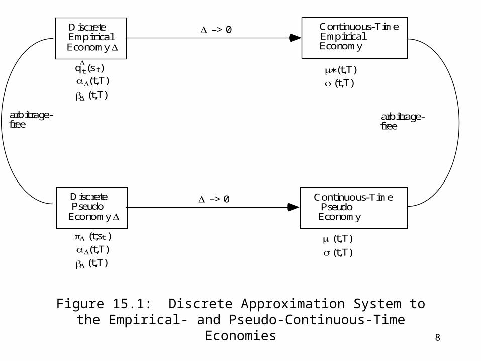
Figure 15.1: Discrete Approximation System to the Empirical- and Pseudo-Continuous-Time Economies. - PowerPoint PPT Presentation
Citation preview
1
15 Continuous-Time Limits This chapter discusses the computer implementation of the interest rate option models developed in the previous chapters. As a discrete-time model, its approximation to reality is good when the number of periods () is large. In this case, the discrete-time model is approximating the continuous trading limit. In fact, for purposes of empirical estimation, it is convenient to reparameterize the discrete-time model in terms of its continuous-time limit. The actual implementation of computer code is then done under this reparameterization. The primary purpose of this chapter is to study this reparameterization and the resulting continuous-time limit. A secondary purpose is to demonstrate how to construct arbitrage-free zero-curve evolutions such as those used in the examples of the previous chapters.
2
A Motivation
This section discusses the intuition behind theconstruction of the discrete time approximation tothe continuous-time limit economy.
To parameterize the forward rate process in termsof its continuous limit, we need to change the timescale in the discrete-time model.
As it is currently constructed, there are timeperiods t = 0, 1, 2,..., . These time periods arearbitrarily specified.
3
I n o r d e r t o t a k e l i m i t s , l e t u s f i x a f u t u r e d a t e ( s a y , J a n u a r y 1 , 2 0 3 0 ) , a n d d i v i d e t h e t i m e h o r i z o n0 t o i n t o s u b p e r i o d s o f e q u a l l e n g t h .
I n t e r m s o f c a l e n d a r t i m e , t h e d i s c r e t e p e r i o d s 0 , 1 ,2 , . . . , c o r r e s p o n d t o t h e d a t e s 0 , , 2 , 3 , . . . ,
.
W e a r e i n t e r e s t e d i n s t u d y i n g t h e v a r i o u sd i s c r e t e - t i m e e c o n o m i e s w h e n t h e n u m b e r o ft r a d i n g d a t e s b e c o m e s l a r g e ( i . e . , ) o r ,e q u i v a l e n t l y , w h e n t h e t i m e b e t w e e n t r a d e sb e c o m e s s m a l l ( i . e . , 0 ) .
4
T h e d i s c r e t e - t i m e f o r w a r d r a t e i s d e n o t e d )T,t(f .
R e c a l l t h a t t h i s r e p r e s e n t s “ o n e p l u s t h ep e r c e n t a g e ” f o r w a r d r a t e a t t i m e t f o r t h e f u t u r et i m e p e r i o d [ T , T + ] .
T h e c o n t i n u o u s l y c o m p o u n d e d ( c o n t i n u o u s - t i m e )f o r w a r d r a t e )T,t(f
~ c o r r e s p o n d s t o t h a t r a t e s u c ht h a t
)T,t(f
~e)T,t(f .
I t i s t h a t r a t e , c o m p o u n d e d c o n t i n u o u s l y f o r u n i t s o f t i m e t h a t e q u a l s t h e d i s c r e t e r a t e .
N o t e t h a t t h i s e x p r e s s i o n i m p l i e s t h a t )T,t(f~ i s a
p e r c e n t a g e .
M o r e f o r m a l l y ,
T,tflog
0lim)T,t(f
~ .
5
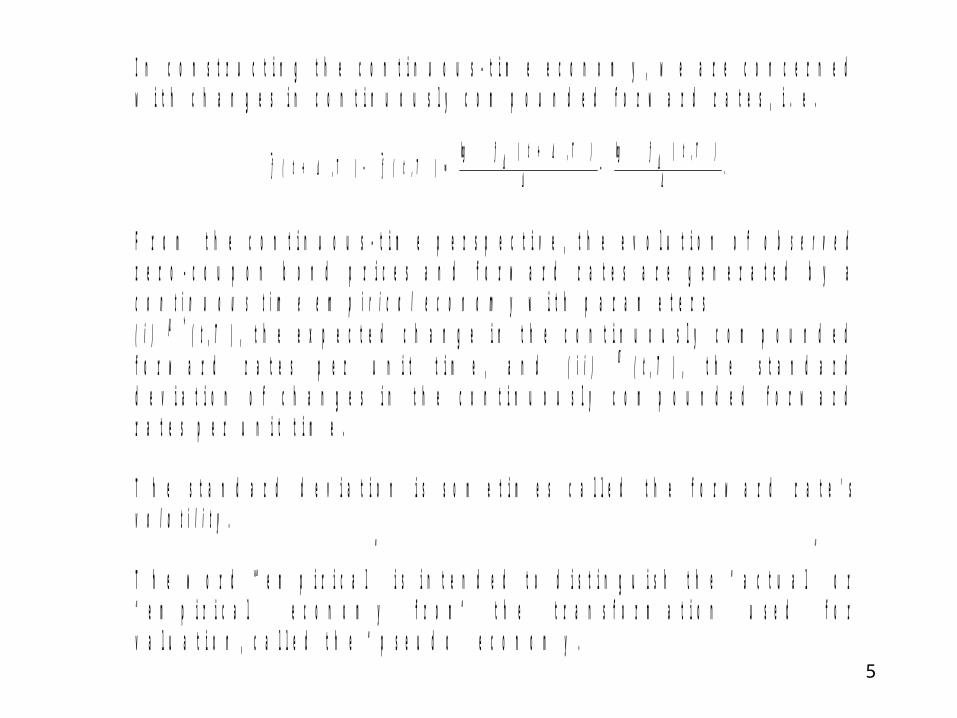
I n c o n s t r u c t i n g t h e c o n t i n u o u s - t i m e e c o n o m y , w e a r e c o n c e r n e dw i t h c h a n g e s i n c o n t i n u o u s l y c o m p o u n d e d f o r w a r d r a t e s , i . e .
.)T,t(flog)T,t(flog
)T,t(f~
)T,t(f~
F r o m t h e c o n t i n u o u s - t i m e p e r s p e c t i v e , t h e e v o l u t i o n o f o b s e r v e dz e r o - c o u p o n b o n d p r i c e s a n d f o r w a r d r a t e s a r e g e n e r a t e d b y ac o n t i n u o u s t i m e e m p i r i c a l e c o n o m y w i t h p a r a m e t e r s( i ) * ( t , T ) , t h e e x p e c t e d c h a n g e i n t h e c o n t i n u o u s l y c o m p o u n d e df o r w a r d r a t e s p e r u n i t t i m e , a n d ( i i ) ( t , T ) , t h e s t a n d a r dd e v i a t i o n o f c h a n g e s i n t h e c o n t i n u o u s l y c o m p o u n d e d f o r w a r dr a t e s p e r u n i t t i m e .
T h e s t a n d a r d d e v i a t i o n i s s o m e t i m e s c a l l e d t h e f o r w a r d r a t e ’ sv o l a t i l i t y .
T h e w o r d “ e m p i r i c a l ” i s i n t e n d e d t o d i s t i n g u i s h t h e “ a c t u a l ” o r“ e m p i r i c a l ” e c o n o m y f r o m t h e t r a n s f o r m a t i o n u s e d f o rv a l u a t i o n , c a l l e d t h e “ p s e u d o ” e c o n o m y .
6
W e w o u l d l i k e t o c o n s t r u c t a n a p p r o x i m a t i n gd i s c r e t e - t i m e e m p i r i c a l e c o n o m y s u c h t h a t a s t h es t e p s i z e s h r i n k s ( 0 ) , t h e d i s c r e t e - t i m ee c o n o m y a p p r o a c h e s t h e c o n t i n u o u s - t i m ee c o n o m y .
R e c a l l t h a t a d i s c r e t e - t i m e e m p i r i c a l e c o n o m y i sc h a r a c t e r i z e d b y( i ) t h e p r o b a b i l i t y o f m o v e m e n t s o f f o r w a r d r a t e s
q
t ( s t ) a n d( i i ) t h e ( o n e p l u s ) p e r c e n t a g e c h a n g e s i n f o r w a r d
r a t e s a c r o s s t h e v a r i o u s s t a t e s( ( t , T ; s t ) , ( t , T ; s t ) f o r t h e o n e - f a c t o r c a s e ) .
7
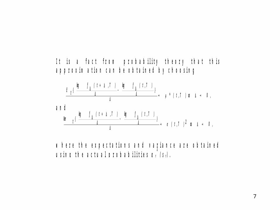
I t i s a f a c t f r o m p r o b a b i l i t y t h e o r y t h a t t h i sa p p r o x i m a t i o n c a n b e o b t a i n e d b y c h o o s i n g
,0 as )T,t(*}
)T,t(flog )T,t(flog {tE
a n d
,0 as 2)T,t(}
)T,t(flog )T,t(flog {tVar
w h e r e t h e e x p e c t a t i o n s a n d v a r i a n c e a r e o b t a i n e du s i n g t h e a c t u a l p r o b a b i l i t i e s q t
( s t ) .
8
Figure 15.1: Discrete Approximation System to the Empirical- and Pseudo-Continuous-Time Economies
Discrete Empirical Economy
Discrete Pseudo
Economy
Continuous-Time Empirical Economy
Continuous-Time Pseudo
Economy
arbitrage- free
–> 0
–> 0
(t;s )
q (s )
(t,T) (t,T)
t
t t
(t,T)
(t,T)
(t,T) (t,T)
(t,T)
(t,T)
arbitrage- free
9
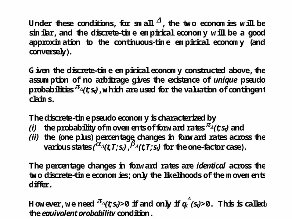
Under these conditions, for small , the two economies will besimilar, and the discrete-time empirical economy will be a goodapproximation to the continuous-time empirical economy (andconversely).
Given the discrete-time empirical economy constructed above, theassumption of no arbitrage gives the existence of unique pseudoprobabilities (t;st), which are used for the valuation of contingentclaims.
The discrete-time pseudo economy is characterized by(i) the probability of movements of forward rates (t;st) and(ii) the (one plus) percentage changes in forward rates across the
various states ((t,T;st), (t,T;st) for the one-factor case).
The percentage changes in forward rates are identical across thetwo discrete-time economies; only the likelihoods of the movementsdiffer.
However, we need (t;st)>0 if and only if qt(st)>0. This is called
the equivalent probability condition.
10
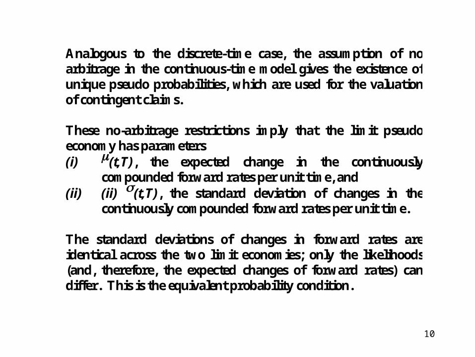
Analogous to the discrete-time case, the assumption of noarbitrage in the continuous-time model gives the existence ofunique pseudo probabilities, which are used for the valuationof contingent claims.
These no-arbitrage restrictions imply that the limit pseudoeconomy has parameters(i) (t,T), the expected change in the continuously
compounded forward rates per unit time, and(ii) (ii) (t,T), the standard deviation of changes in the
continuously compounded forward rates per unit time.
The standard deviations of changes in forward rates areidentical across the two limit economies; only the likelihoods(and, therefore, the expected changes of forward rates) candiffer. This is the equivalent probability condition.
11
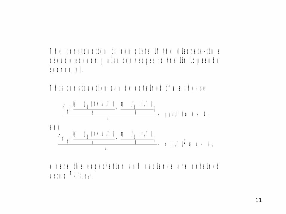
T h e c o n s t r u c t i o n i s c o m p l e t e i f t h e d i s c r e t e - t i m ep s e u d o e c o n o m y a l s o c o n v e r g e s t o t h e l i m i t p s e u d oe c o n o m y ) .
T h i s c o n s t r u c t i o n c a n b e o b t a i n e d i f w e c h o o s e
,0 as )T,t(}
)T,t(flog )T,t(flog {tE
~
a n d
,0 as 2)T,t(}
)T,t(flog )T,t(flog {tarV
~
w h e r e t h e e x p e c t a t i o n a n d v a r i a n c e a r e o b t a i n e du s i n g ( t ; s t ) .
12
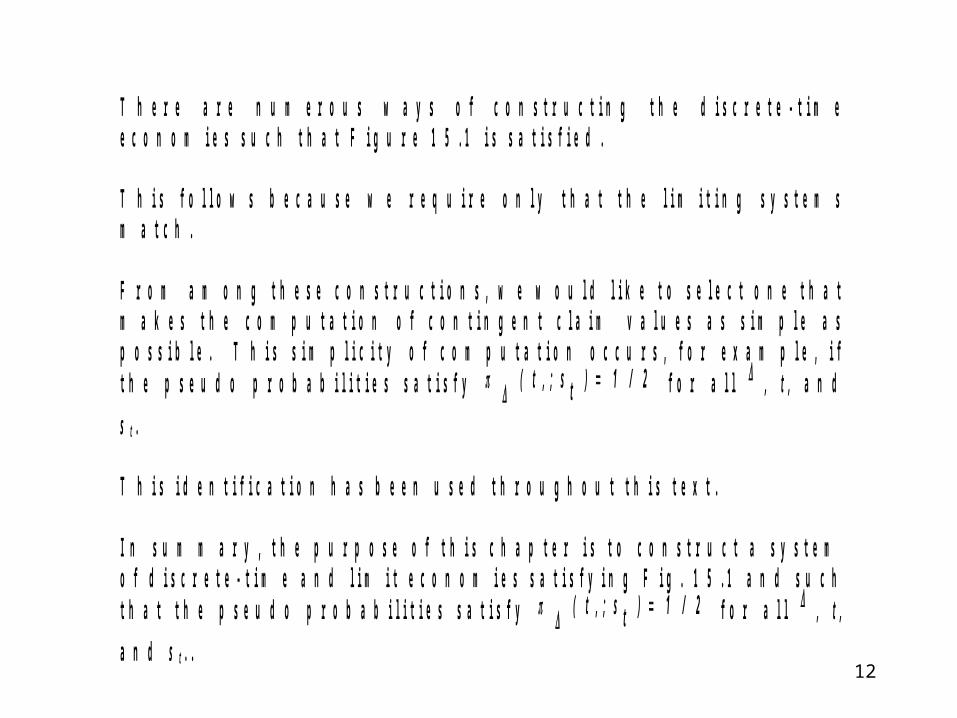
T h e r e a r e n u m e r o u s w a y s o f c o n s t r u c t i n g t h e d i s c r e t e - t i m e e c o n o m i e s s u c h t h a t F i g u r e 1 5 . 1 i s s a t i s f i e d . T h i s f o l l o w s b e c a u s e w e r e q u i r e o n l y t h a t t h e l i m i t i n g s y s t e m s m a t c h . F r o m a m o n g t h e s e c o n s t r u c t i o n s , w e w o u l d l i k e t o s e l e c t o n e t h a t m a k e s t h e c o m p u t a t i o n o f c o n t i n g e n t c l a i m v a l u e s a s s i m p l e a s p o s s i b l e . T h i s s i m p l i c i t y o f c o m p u t a t i o n o c c u r s , f o r e x a m p l e , i f t h e p s e u d o p r o b a b i l i t i e s s a t i s f y 2/1)ts;,t( f o r a l l , t , a n d
s t . T h i s i d e n t i f i c a t i o n h a s b e e n u s e d t h r o u g h o u t t h i s t e x t . I n s u m m a r y , t h e p u r p o s e o f t h i s c h a p t e r i s t o c o n s t r u c t a s y s t e m o f d i s c r e t e - t i m e a n d l i m i t e c o n o m i e s s a t i s f y i n g F i g . 1 5 . 1 a n d s u c h t h a t t h e p s e u d o p r o b a b i l i t i e s s a t i s f y 2/1)ts;,t( f o r a l l , t ,
a n d s t . .
13
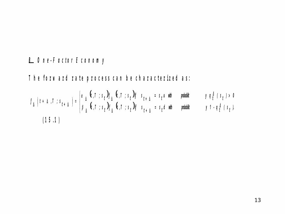
B O n e - F a c t o r E c o n o m y T h e f o r w a r d r a t e p r o c e s s c a n b e c h a r a c t e r i z e d a s :
).ts(tq-1y probabilit with dtsts if ts;T,tfts;T,t
0)ts(tqy probabilit with utsts if ts;T,tfts;T,t
ts;T,tf
( 1 5 . 1 )
14
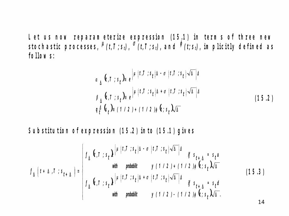
L e t u s n o w r e p a r a m e t e r i z e e x p r e s s i o n ( 1 5 . 1 ) i n t e r m s o f t h r e e n e w s t o c h a s t i c p r o c e s s e s , ( t , T ; s t ) , ( t , T ; s t ) , a n d ( t ; s t ) , i m p l i c i t l y d e f i n e d a s f o l l o w s :
ts;t)2/1()2/1(tstq
ts;T,tts;T,tets;T,t
ts;T,tts;T,tets;T,t
( 1 5 . 2 )
S u b s t i t u t i o n o f e x p r e s s i o n ( 1 5 . 2 ) i n t o ( 1 5 . 1 ) g i v e s
.ts;t)2/1()2/1(y probabilit with
dts=tsifts;T,tts;T,tets;T,tf
ts;t)2/1()2/1(y probabilit with
uts=tsifts;T,tts;T,tets;T,tf
ts;T,tf
( 1 5 . 3 )
15
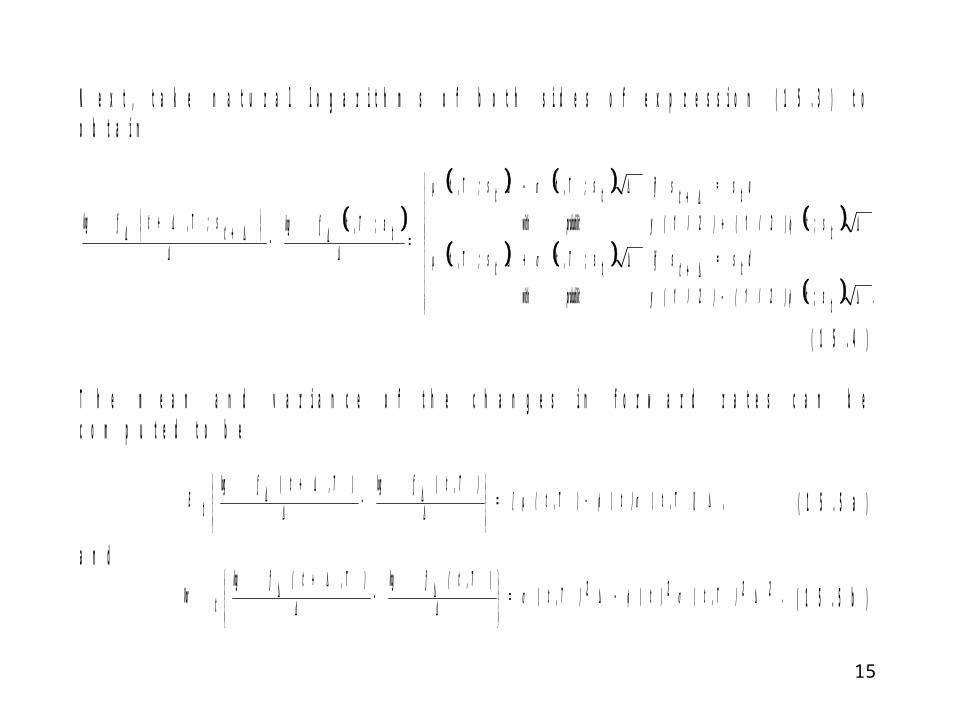
N e x t , t a k e n a t u r a l l o g a r i t h m s o f b o t h s i d e s o f e x p r e s s i o n ( 1 5 . 3 ) t o o b t a i n
.ts;t)2/1()2/1(y pr obabilit w ith
dts=tsifts;T,tts;T,tts;t)2/1()2/1(y pr obabilit w ith
uts=tsifts;T,tts;T,t
ts;T,tflogts;T,tflog
( 1 5 . 4 ) T h e m e a n a n d v a r i a n c e o f t h e c h a n g e s i n f o r w a r d r a t e s c a n b e c o m p u t e d t o b e
,)]T,t()t()T,t([)T,t(flog )T,t(flog
tE
( 1 5 . 5 a )
a n d
.22)T,t(2)t(2)T,t()T,t(flog )T,t(flog
tVar
( 1 5 . 5 b )
16
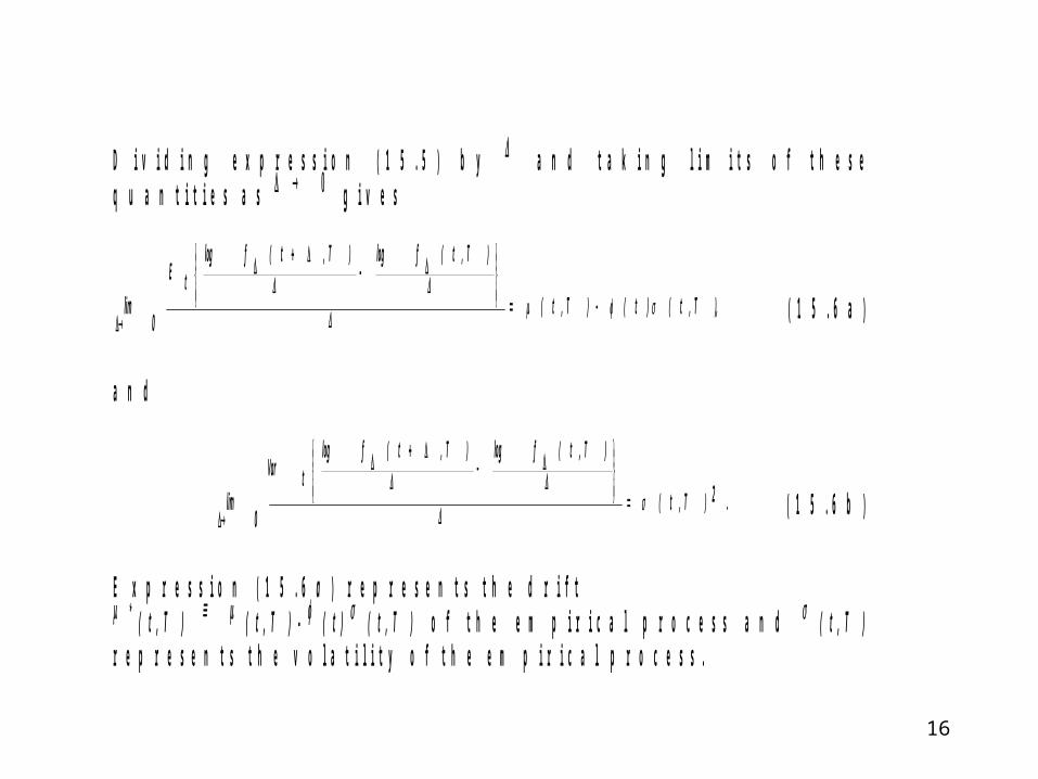
D i v i d i n g e x p r e s s i o n ( 1 5 . 5 ) b y a n d t a k i n g l i m i t s o f t h e s e q u a n t i t i e s a s g i v e s
),T,t()t()T,t(
)T,t(flog )T,t(flog tE
0lim
( 1 5 . 6 a )
a n d
.2)T,t(
)T,t(flog )T,t(flog tVar
0lim
( 1 5 . 6 b )
E x p r e s s i o n ( 1 5 . 6 a ) r e p r e s e n t s t h e d r i f t * ( t , T ) ( t , T ) - ( t ) ( t , T ) o f t h e e m p i r i c a l p r o c e s s a n d ( t , T ) r e p r e s e n t s t h e v o l a t i l i t y o f t h e e m p i r i c a l p r o c e s s .
17
Both *(t,T) and (t,T) can in principle be estimated from past observations of forward rates. The stochastic process (t) can be interpreted as a risk premium, i.e., a measure of the excess expected return (above the spot rate) per unit of standard deviation for the zero-coupon bonds. The parameterization of the empirical discrete-time process as given in expression (15.2), therefore, is an approximation to the empirical continuous economy with drift *(t,T) (t,T)-(t)(t,T) and volatility (t,T).
18
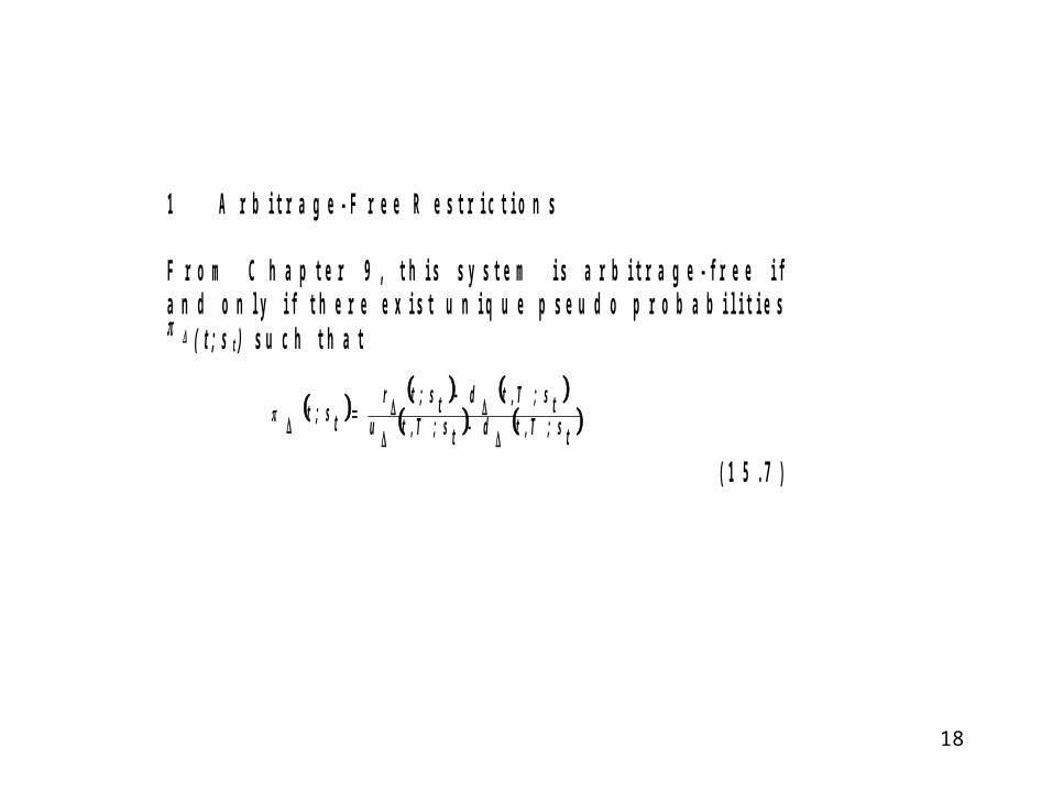
1 A r b i t r a g e - F r e e R e s t r i c t i o n s F r o m C h a p t e r 9 , t h i s s y s t e m i s a r b i t r a g e - f r e e i f a n d o n l y i f t h e r e e x i s t u n i q u e p s e u d o p r o b a b i l i t i e s ( t ; s t ) s u c h t h a t
ts;T,tdts;T,tu
ts;T,tdts;trts;t
( 1 5 . 7 )
19
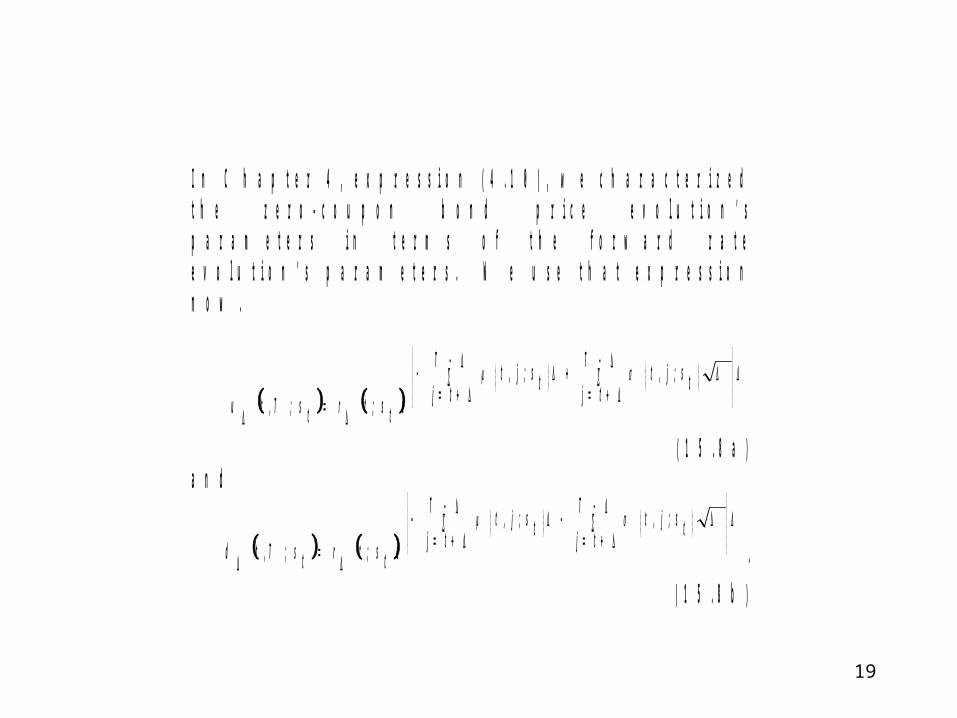
I n C h a p t e r 4 , e x p r e s s i o n ( 4 . 1 0 ) , w e c h a r a c t e r i z e d t h e z e r o - c o u p o n b o n d p r i c e e v o l u t i o n ’ s p a r a m e t e r s i n t e r m s o f t h e f o r w a r d r a t e e v o l u t i o n ’ s p a r a m e t e r s . W e u s e t h a t e x p r e s s i o n n o w .
ts;j,tT
tjts;j,t
T
tjets;trts;T,tu
( 1 5 . 8 a ) a n d
ts;j,tT
tjts;j,t
T
tjets;trts;T,td .
( 1 5 . 8 b )
20
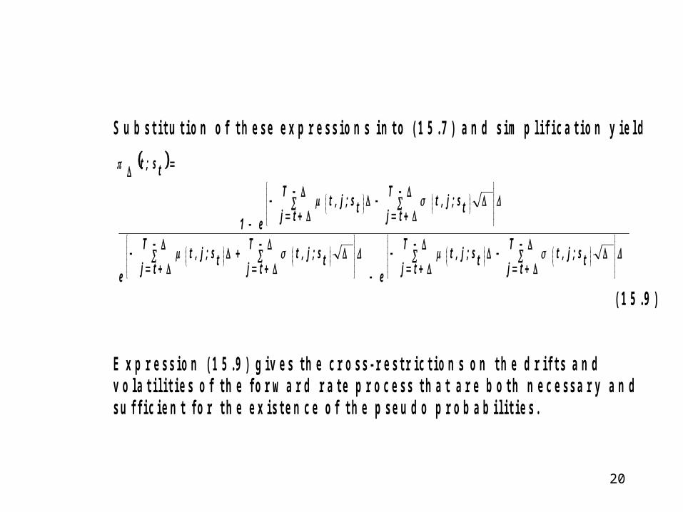
S u b s t i t u t i o n o f t h e s e e x p r e s s i o n s i n t o ( 1 5 . 7 ) a n d s i m p l i f i c a t i o n y i e l d
ts;j,tT
tjts;j,t
T
tjets;j,t
T
tjts;j,t
T
tje
ts;j,tT
tjts;j,t
T
tje1
ts;t
( 1 5 . 9 ) E x p r e s s i o n ( 1 5 . 9 ) g i v e s t h e c r o s s - r e s t r i c t i o n s o n t h e d r i f t s a n d v o l a t i l i t i e s o f t h e f o r w a r d r a t e p r o c e s s t h a t a r e b o t h n e c e s s a r y a n d s u f f i c i e n t f o r t h e e x i s t e n c e o f t h e p s e u d o p r o b a b i l i t i e s .
21
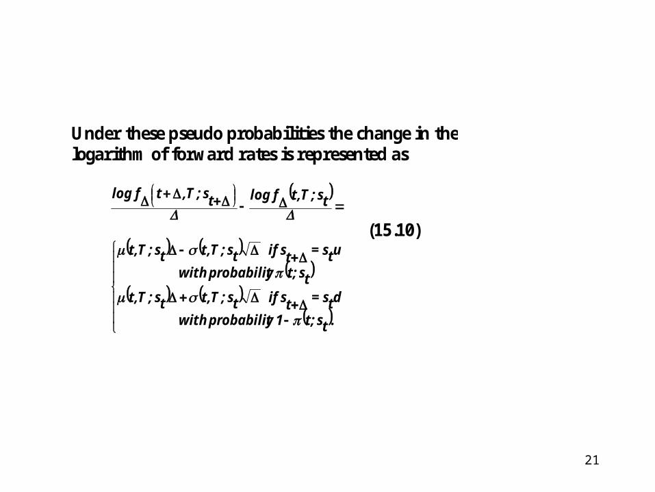
Under these pseudo probabilities the change in the logarithm of forward rates is represented as
.ts;t1y probabilit with
dts=tsifts;T,tts;T,tts;ty probabilit with
uts=tsifts;T,tts;T,t
ts;T,tflogts;T,tflog
(15.10)
22
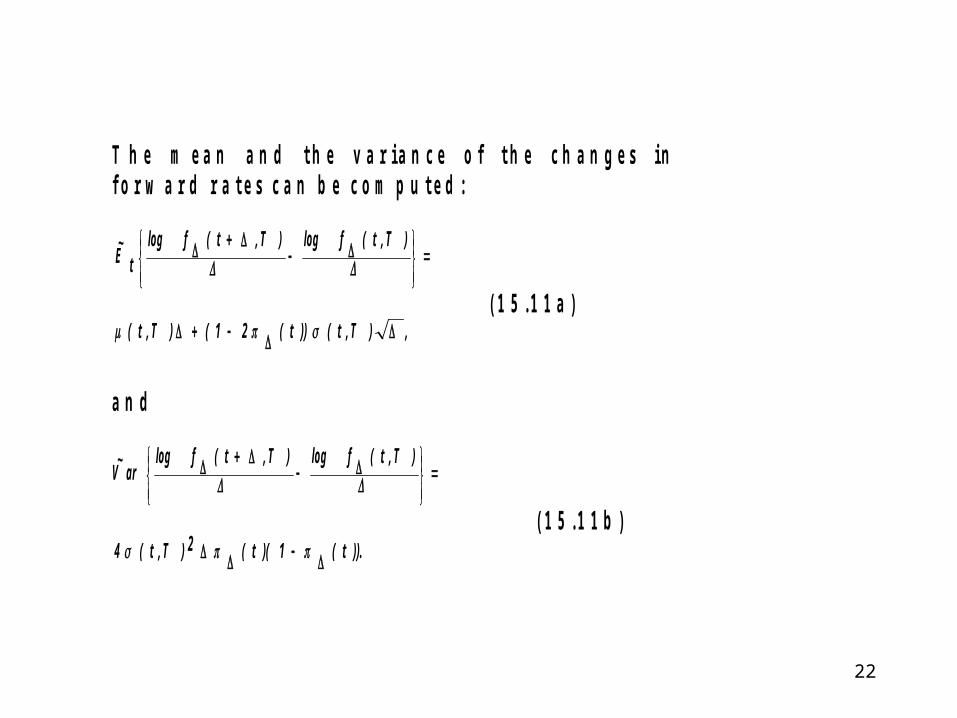
T h e m e a n a n d t h e v a r i a n c e o f t h e c h a n g e s i n f o r w a r d r a t e s c a n b e c o m p u t e d :
,)T,t())t(21()T,t(
)T,t(flog )T,t(flog tE
~
( 1 5 . 1 1 a )
a n d
)).t(1)(t(2)T,t(4
)T,t(flog )T,t(flog arV
~
( 1 5 . 1 1 b )
23
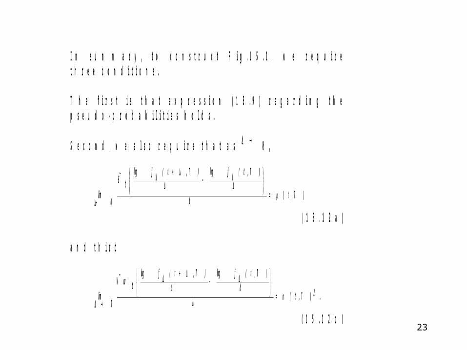
I n s u m m a r y , t o c o n s t r u c t F i g . 1 5 . 1 , w e r e q u i r e t h r e e c o n d i t i o n s . T h e f i r s t i s t h a t e x p r e s s i o n ( 1 5 . 9 ) r e g a r d i n g t h e p s e u d o - p r o b a b i l i t i e s h o l d s . S e c o n d , w e a l s o r e q u i r e t h a t a s 0 ,
)T,t(
)T,t(flog )T,t(flog tE
~
0lim
( 1 5 . 1 2 a ) a n d t h i r d
.2)T,t(
)T,t(flog )T,t(flog tarV
~
0lim
( 1 5 . 1 2 b )
24
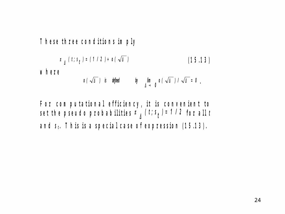
T h e s e t h r e e c o n d i t i o n s i m p l y
)(o)2/1()ts;t( ( 1 5 . 1 3 )
w h e r e 0/)(o
0limbydefinedis)(o
.
F o r c o m p u t a t i o n a l e f f i c i e n c y , i t i s c o n v e n i e n t t o s e t t h e p s e u d o p r o b a b i l i t i e s 2/1)ts;t( f o r a l l t
a n d s t . T h i s i s a s p e c i a l c a s e o f e x p r e s s i o n ( 1 5 . 1 3 ) .
25
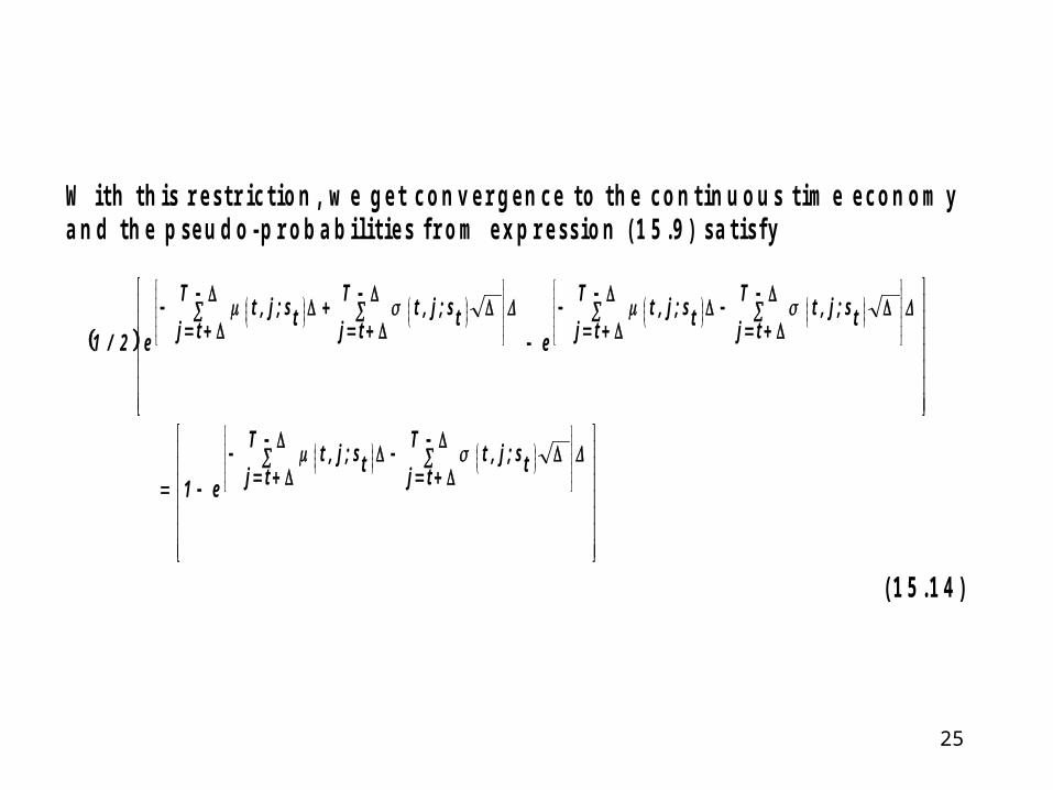
W i t h t h i s r e s t r i c t i o n , w e g e t c o n v e r g e n c e t o t h e c o n t i n u o u s t i m e e c o n o m y a n d t h e p s e u d o - p r o b a b i l i t i e s f r o m e x p r e s s i o n ( 1 5 . 9 ) s a t i s f y
ts;j,tT
tjts;j,t
T
tje1
ts;j,tT
tjts;j,t
T
tjets;j,t
T
tjts;j,t
T
tje2/1
( 1 5 . 1 4 )
26
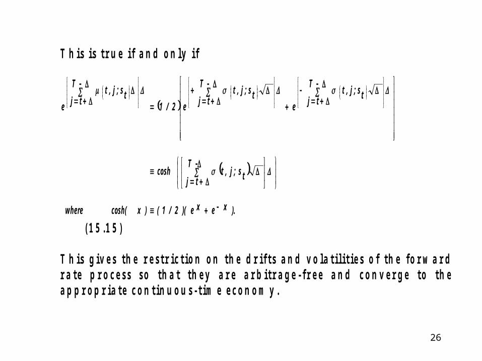
T h i s i s t r u e i f a n d o n l y i f
).xexe)(2/1()xcosh(where
ts;j,tT
tjcosh
ts;j,tT
tjets;j,t
T
tje2/1ts;j,t
T
tje
( 1 5 . 1 5 ) T h i s g i v e s t h e r e s t r i c t i o n o n t h e d r i f t s a n d v o l a t i l i t i e s o f t h e f o r w a r d r a t e p r o c e s s s o t h a t t h e y a r e a r b i t r a g e - f r e e a n d c o n v e r g e t o t h e a p p r o p r i a t e c o n t i n u o u s - t i m e e c o n o m y .
27
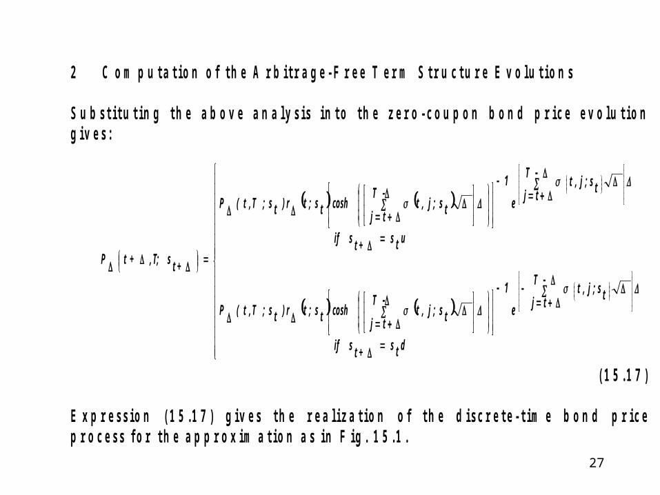
2 C o m p u t a t i o n o f t h e A r b i t r a g e - F r e e T e r m S t r u c t u r e E v o l u t i o n s S u b s t i t u t i n g t h e a b o v e a n a l y s i s i n t o t h e z e r o - c o u p o n b o n d p r i c e e v o l u t i o n g i v e s :
dts+ts if
ts;j,t
T
tje
1
ts;j,tT
tjcoshts;tr)ts;T,t(P
uts+ts if
ts;j,t
T
tje
1
ts;j,tT
tjcoshts;tr)ts;T,t(P
+tsT;,+tP
( 1 5 . 1 7 ) E x p r e s s i o n ( 1 5 . 1 7 ) g i v e s t h e r e a l i z a t i o n o f t h e d i s c r e t e - t i m e b o n d p r i c e p r o c e s s f o r t h e a p p r o x i m a t i o n a s i n F i g . 1 5 . 1 .
28
Under the em pirical probabilities )ts;t()2/1()2/1( , this bond
price process converges to the limiting empirical process forthe bond's price.Under the pseudo probabilities )2/1()ts;t( , this converges to
the limiting pseudo process for the bond's price.
29
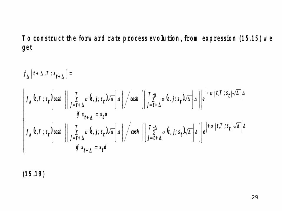
T o c o n s t r u c t t h e f o r w a r d r a t e p r o c e s s e v o l u t i o n , f r o m e x p r e s s i o n ( 1 5 . 1 5 ) w e g e t
dtstsif
ts;T,tets;j,t
T
tjcoshts;j,t
T
tjcoshts;T,tf
utstsif
ts;T,tets;j,t
T
tjcoshts;j,t
T
tjcoshts;T,tf
ts;T,tf
( 1 5 . 1 9 )
30
U n d e r t h e e m p i r i c a l p r o b a b i l i t i e s)ts;t()2/1()2/1( , t h i s p r o c e s s c o n v e r g e s t o
t h e e m p i r i c a l c o n t i n u o u s - t i m e p r o c e s s f o r t h ef o r w a r d r a t e s .
U n d e r t h e p s e u d o p r o b a b i l i t i e s )2/1()ts;t( ,
t h i s c o n v e r g e s t o t h e p s e u d o c o n t i n u o u s - t i m ep r o c e s s f o r t h e f o r w a r d r a t e s .
31
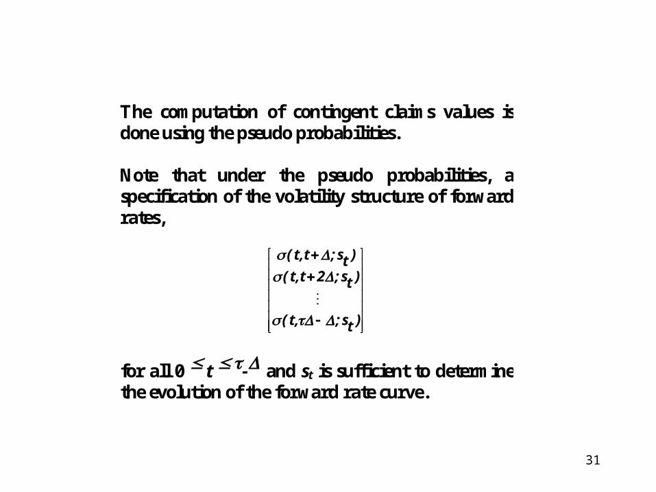
The computation of contingent claims values isdone using the pseudo probabilities.
Note that under the pseudo probabilities, aspecification of the volatility structure of forwardrates,
)ts;,t(
)ts;2t,t(
)ts;t,t(
for all 0 t - and st is sufficient to determinethe evolution of the forward rate curve.
32
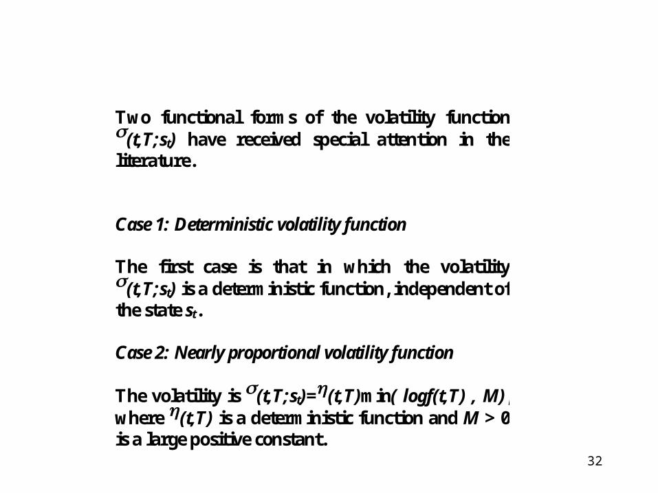
Two functional forms of the volatility function(t,T;st) have received special attention in theliterature.
Case 1: Deterministic volatility function
The first case is that in which the volatility(t,T;st) is a deterministic function, independent ofthe state st.
Case 2: Nearly proportional volatility function
The volatility is (t,T;st)=(t,T)min( logf(t,T) , M),where (t,T) is a deterministic function and M > 0is a large positive constant.
33
EXAMPLE: CONSTRUCTION OF FIG. 4.6. To construct Fig. 4.6, we used expression (15.19), with 1 and the following forward rates:
f(0,0)=f(0,1)=f(0,2)=f(0,3)=1.02. We used the volatility function given in case 2 with the proportionality coefficient (t,T) (T-t) depending only on time to maturity and having the values
(1) = .11765, (2) = .08825, and (3) = .06865.
We set M=1,000,000. This completes the example.
34
D Multiple-Factor Economies
The previous analysis is easily extended to N 2-factor economies.
35
E Computational Issues 1 Bushy Trees The procedure provided for computing forward rate curve evolutions in expression (15.19) is called a bushy tree because the number of branches on the tree expands exponentially as the number of time steps increases. For large numbers of time steps, depending upon what computational tricks are employed, the computing time becomes excessive. For this reason it is often incorrectly believed that contingent claim valuation cannot be done using bushy trees. This belief is incorrect because a large number of time steps is not always essential for obtaining good approximations
36
For European options or American options withsix or seven decision nodes (of economicimportance), bushy trees provide very accuratevalues with step sizes of only 12-14. This isbecause the branches spread out very quickly,giving a fine grid of values at the last date in thetree. From a numerical integration perspective(recall valuation is equivalent to computing anexpected value), the approximating grid at the lastdate will be quite accurate.
For exotic options with multiple cash flow times(say 14) or long-dated American options withmany decision nodes of economic importance(say 14), bushy trees provide a less attractive,time-intensive computational procedure.
37
2 Lattices
Special cases of the one-factor model allow for more efficient computation. These are the cases in which the tree recombines at various nodes.
For the one-factor economy, the tree recombines when the volatilityfunction (t,T) is a constant, independent of either time or the maturitydate. Furthermore, under a time transformation, case 1 (the deterministicvolatility function), can also be shown to recombine.
Given the pseudo probabilities, the spot rate process itself is sufficient todetermine the zero-coupon bond prices and therefore forward rates.
38
The spot rate process can be made to recombine under varioustransformations. These transformations work well for the one-factor case.More research is needed for the multifactor case from a lattice approach.
One-factor lattice approaches work well for most contingent claims, exceptthose that are path dependent, e.g., index-amortizing swaps. This is becausea lattice does not remember the path taken through the tree, but only thecurrent node. For path-dependent options, bushy trees and Monte Carlosimulation appear to be better approaches.
39
3 Partial Differential Equations
Numerical techniques are quite refined for solving partial differentialequations, by either implicit or explicit difference techniques.
These techniques can be applied to price interest rate options when thespot rate process is (strong) Markov in a finite number of statevariables.
When the spot rate process is (strong) Markov, the use of Ito's lemma(from stochastic calculus) enables one to transform the expected valuerelation to a partial differential equation subject to boundaryconditions.
A limitation of this approach is that it cannot easily handlepath-dependent options, such as index-amortizing swaps.
40
1
4 Monte Carlo Simulation
As stated earlier, contingent claims valuation reducesto calculating an expected value given thearbitrage-free evolution of the term structure ofinterest rates.
Monte Carlo techniques are well suited for suchcomputations. These techniques appear to beespecially well suited for multiple-factor models(greater then 3), in which computations using bushytrees are time-consuming.
Because Monte Carlo simulation is a forward-lookingtechnique, it has some difficulty handling Americanoptions.

![15.1(1) SWIMMINGPOOLSANDSPAS 15.1(2) · IAC6/3/09 PublicHealth[641] Ch15,p.1 CHAPTER15 SWIMMINGPOOLSANDSPAS 641—15.1(135I)Applicability. 15.1(1) Theserulesapplytoswimmingpools,spas,wadingpools,waterslides](https://img.pdfslide.us/doc/110x75/5f08ea2d7e708231d42456b9/1511-swimmingpoolsandspas-1512-iac6309-publichealth641-ch15p1-chapter15.jpg)


![Pseudo-binomial Approximation to k ,k -runsbinomial convoluted Poisson approximation to (1,1)-runs. For more details and applications of runs, see Aki et al. [2], Antzoulakos et al](https://img.pdfslide.us/doc/110x75/608d71d9ba410c056a41c885/pseudo-binomial-approximation-to-k-k-runs-binomial-convoluted-poisson-approximation.jpg)