FIGURE 14.1 TALLEY Surface circulation schematic. This figure can also be found in the color insert. Copyright © 2011 Elsevier Inc. All rights reserved

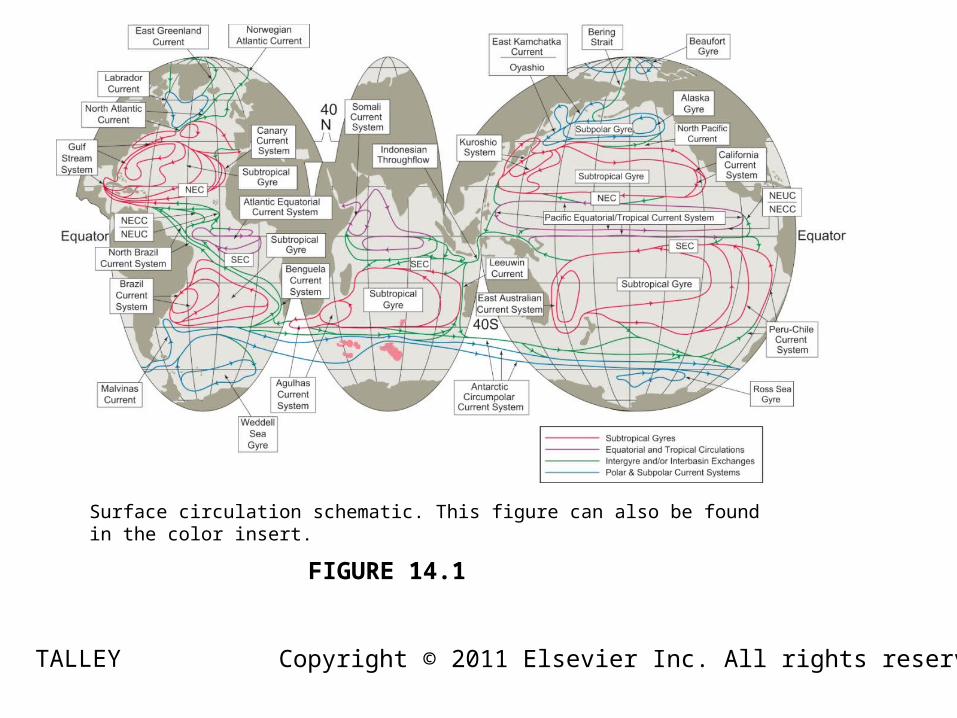
FIGURE 14.1

TALLEY

Surface circulation schematic. This figure can also be found in the color insert.

Copyright © 2011 Elsevier Inc. All rights reserved

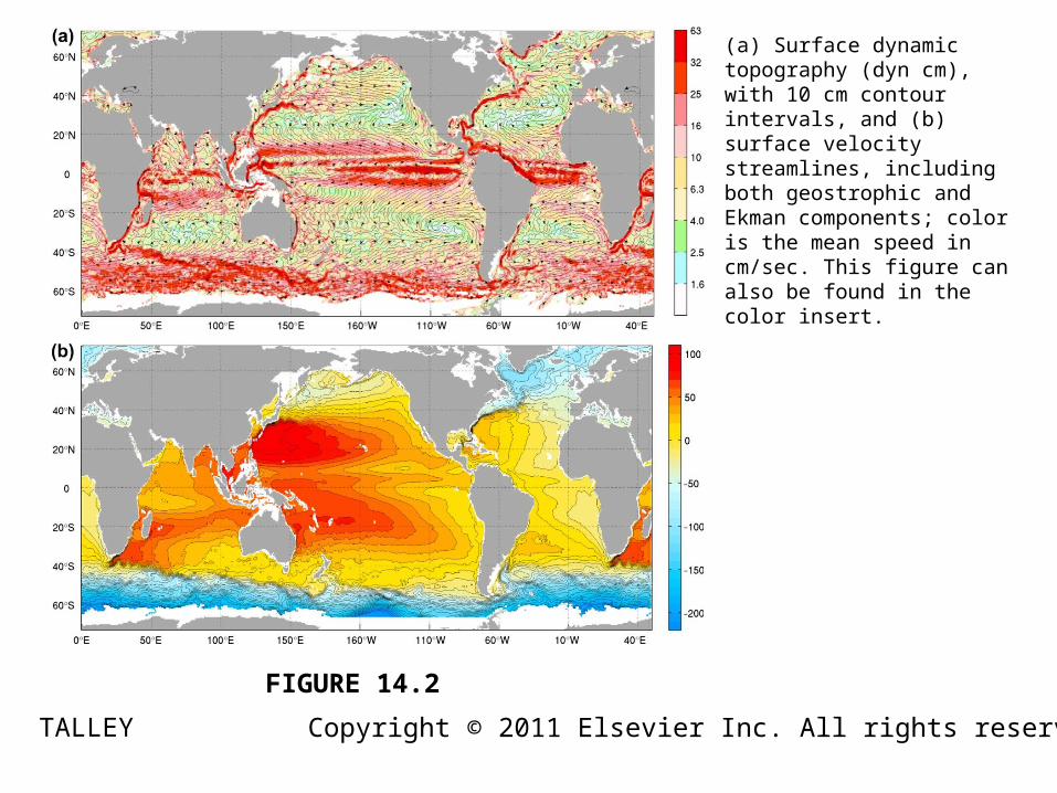
FIGURE 14.2

TALLEY

(a) Surface dynamic topography (dyn cm), with 10 cm contour intervals, and (b) surface velocity streamlines, including both geostrophic and Ekman components; color is the mean speed in cm/sec. This figure can also be found in the color insert.


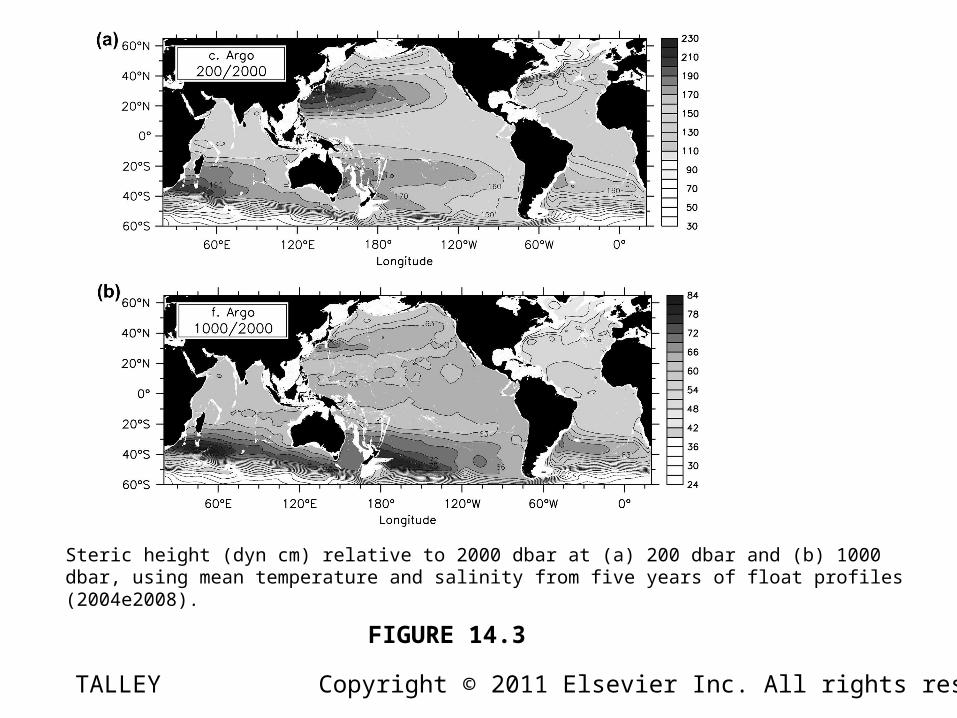
FIGURE 14.3

TALLEY

Steric height (dyn cm) relative to 2000 dbar at (a) 200 dbar and (b) 1000 dbar, using mean temperature and salinity from five years of float profiles (2004e2008).


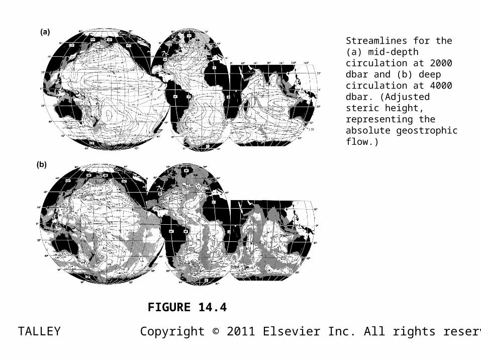
FIGURE 14.4

TALLEY

Streamlines for the (a) mid-depth circulation at 2000 dbar and (b) deep circulation at 4000 dbar. (Adjusted steric height, representing the absolute geostrophic flow.)


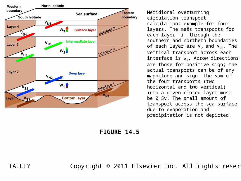
FIGURE 14.5

TALLEY

Meridional overturning circulation transport calculation: example for four layers. The mass transports for each layer “i” through the southern and northern boundaries of each layer are VSi and VNi. The vertical transport across each interface is Wi. Arrow directions are those for positive sign; the actual transports can be of any magnitude and sign. The sum of the four transports (two horizontal and two vertical) into a given closed layer must be 0 Sv. The small amount of transport across the sea surface due to evaporation and precipitation is not depicted.


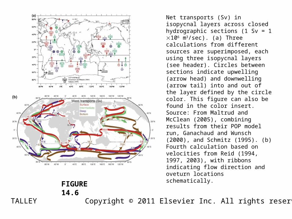
FIGURE 14.6

TALLEY

Net transports (Sv) in isopycnal layers across closed hydrographic sections (1 Sv = 1 106 m3/sec). (a) Three calculations from different sources are superimposed, each using three isopycnal layers (see header). Circles between sections indicate upwelling (arrow head) and downwelling (arrow tail) into and out of the layer defined by the circle color. This figure can also be found in the color insert. Source: From Maltrud and McClean (2005), combining results from their POP model run, Ganachaud and Wunsch (2000), and Schmitz (1995). (b) Fourth calculation based on velocities from Reid (1994, 1997, 2003), with ribbons indicating flow direction and oveturn locations schematically.


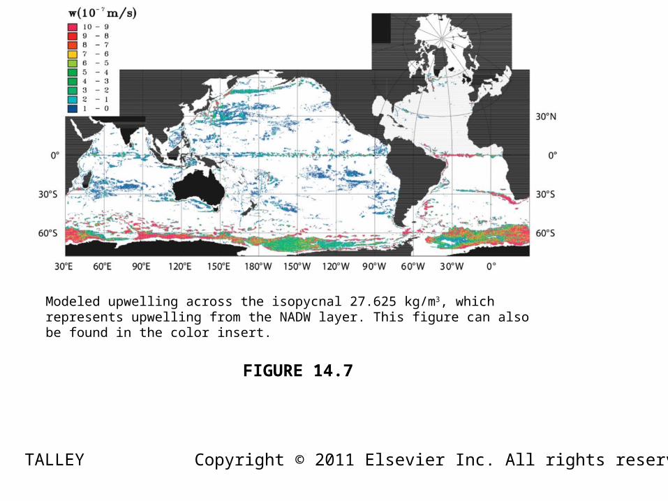
FIGURE 14.7

TALLEY

Modeled upwelling across the isopycnal 27.625 kg/m3, which represents upwelling from the NADW layer. This figure can also be found in the color insert.


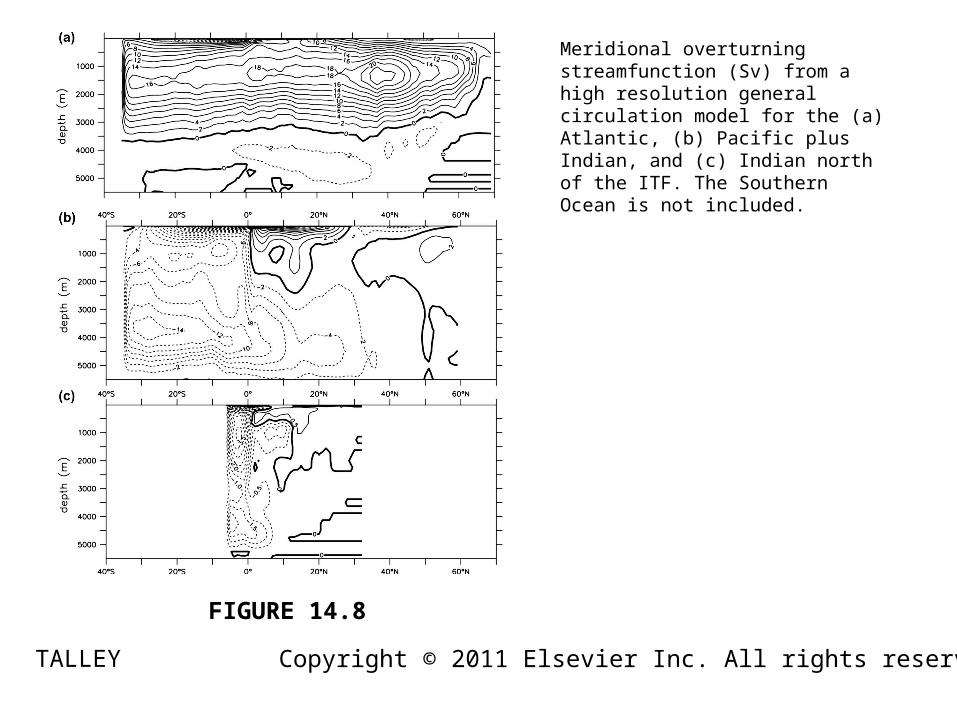
FIGURE 14.8

TALLEY

Meridional overturning streamfunction (Sv) from a high resolution general circulation model for the (a) Atlantic, (b) Pacific plus Indian, and (c) Indian north of the ITF. The Southern Ocean is not included.


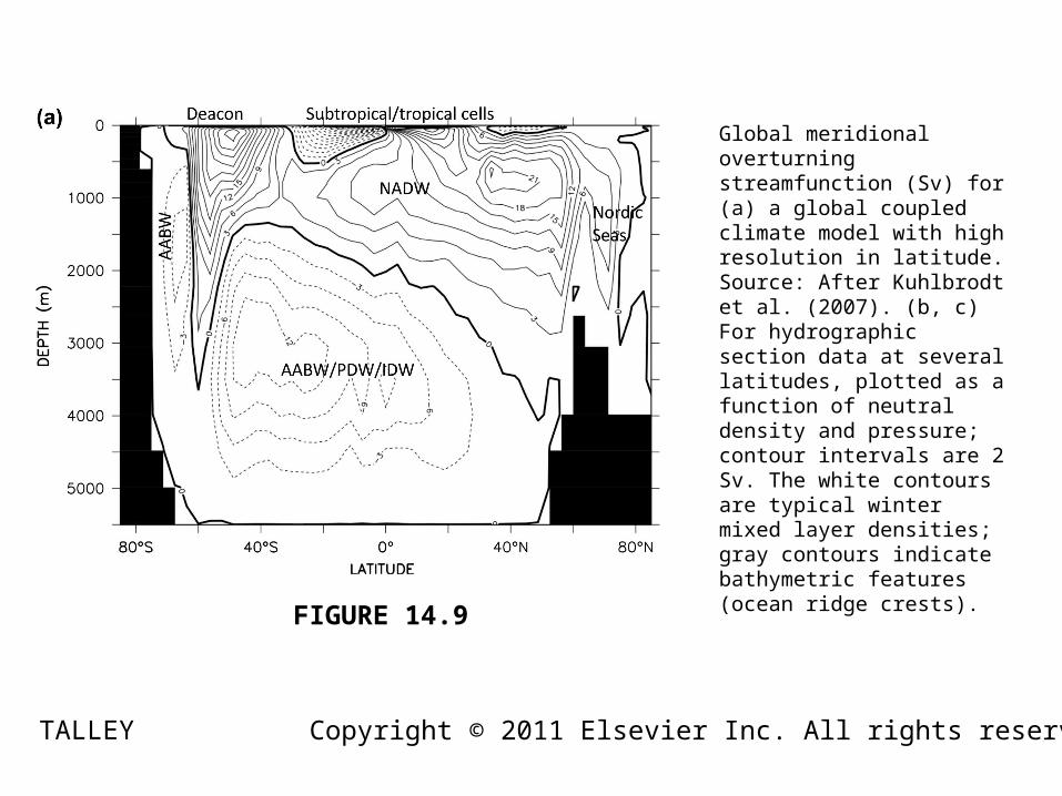
FIGURE 14.9

TALLEY

Global meridional overturning streamfunction (Sv) for (a) a global coupled climate model with high resolution in latitude. Source: After Kuhlbrodt et al. (2007). (b, c) For hydrographic section data at several latitudes, plotted as a function of neutral density and pressure; contour intervals are 2 Sv. The white contours are typical winter mixed layer densities; gray contours indicate bathymetric features (ocean ridge crests).


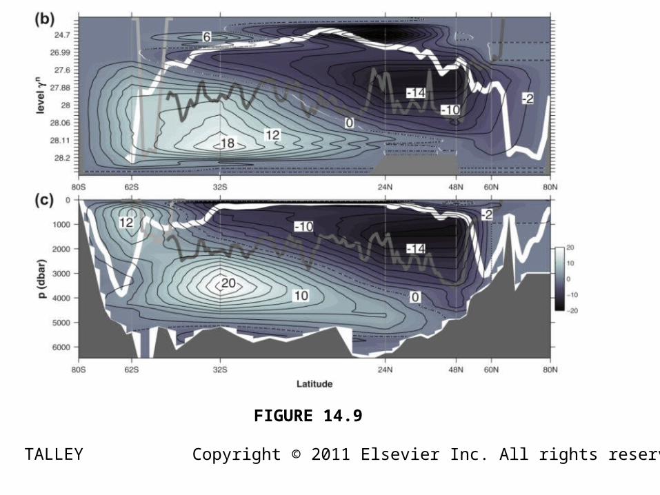
FIGURE 14.9

TALLEY Copyright © 2011 Elsevier Inc. All rights reserved

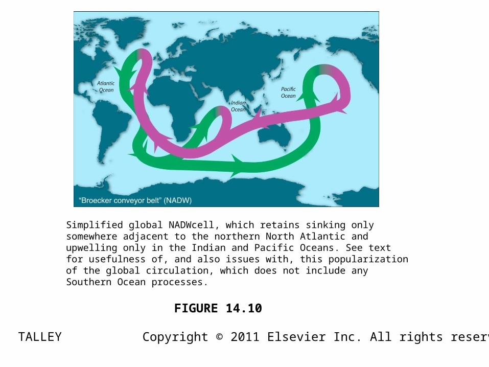
FIGURE 14.10

TALLEY

Simplified global NADWcell, which retains sinking only somewhere adjacent to the northern North Atlantic and upwelling only in the Indian and Pacific Oceans. See text for usefulness of, and also issues with, this popularization of the global circulation, which does not include any Southern Ocean processes.


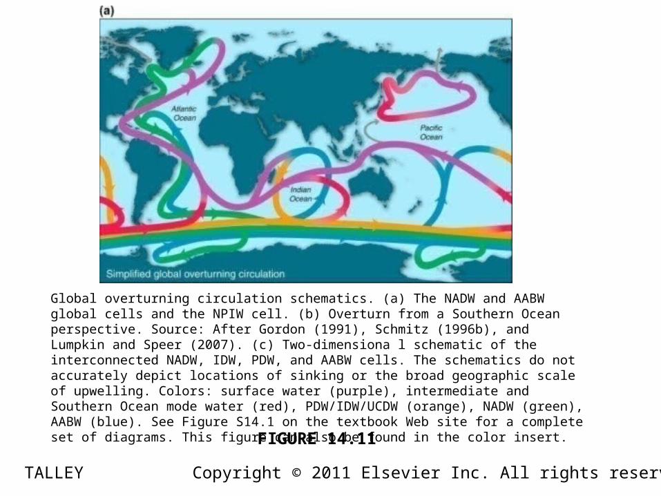
FIGURE 14.11

TALLEY

Global overturning circulation schematics. (a) The NADW and AABW global cells and the NPIW cell. (b) Overturn from a Southern Ocean perspective. Source: After Gordon (1991), Schmitz (1996b), and Lumpkin and Speer (2007). (c) Two-dimensiona l schematic of the interconnected NADW, IDW, PDW, and AABW cells. The schematics do not accurately depict locations of sinking or the broad geographic scale of upwelling. Colors: surface water (purple), intermediate and Southern Ocean mode water (red), PDW/IDW/UCDW (orange), NADW (green), AABW (blue). See Figure S14.1 on the textbook Web site for a complete set of diagrams. This figure can also be found in the color insert.


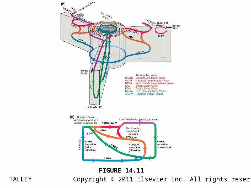
FIGURE 14.11


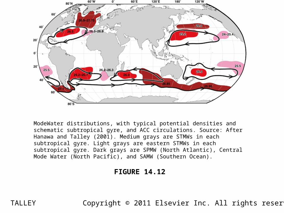
FIGURE 14.12

TALLEY

ModeWater distributions, with typical potential densities and schematic subtropical gyre, and ACC circulations. Source: After Hanawa and Talley (2001). Medium grays are STMWs in each subtropical gyre. Light grays are eastern STMWs in each subtropical gyre. Dark grays are SPMW (North Atlantic), Central Mode Water (North Pacific), and SAMW (Southern Ocean).


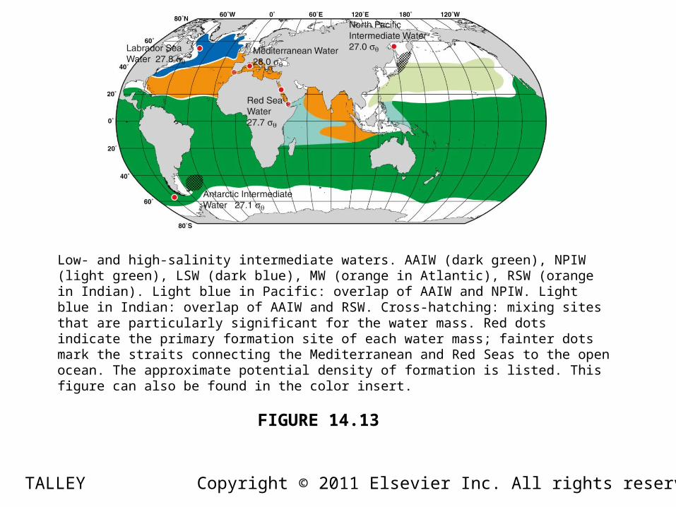
FIGURE 14.13

TALLEY

Low- and high-salinity intermediate waters. AAIW (dark green), NPIW (light green), LSW (dark blue), MW (orange in Atlantic), RSW (orange in Indian). Light blue in Pacific: overlap of AAIW and NPIW. Light blue in Indian: overlap of AAIW and RSW. Cross-hatching: mixing sites that are particularly significant for the water mass. Red dots indicate the primary formation site of each water mass; fainter dots mark the straits connecting the Mediterranean and Red Seas to the open ocean. The approximate potential density of formation is listed. This figure can also be found in the color insert.


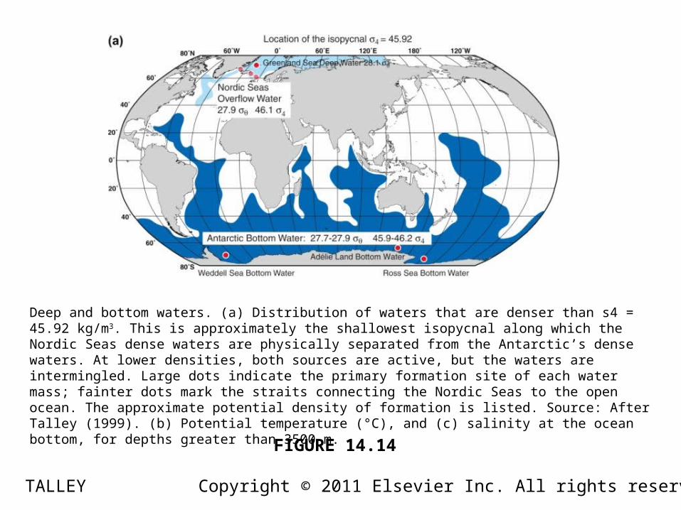
FIGURE 14.14

TALLEY

Deep and bottom waters. (a) Distribution of waters that are denser than s4 = 45.92 kg/m3. This is approximately the shallowest isopycnal along which the Nordic Seas dense waters are physically separated from the Antarctic’s dense waters. At lower densities, both sources are active, but the waters are intermingled. Large dots indicate the primary formation site of each water mass; fainter dots mark the straits connecting the Nordic Seas to the open ocean. The approximate potential density of formation is listed. Source: After Talley (1999). (b) Potential temperature (°C), and (c) salinity at the ocean bottom, for depths greater than 3500 m.


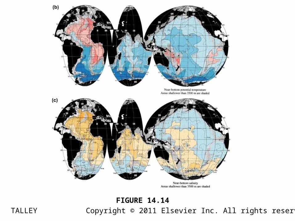
FIGURE 14.14


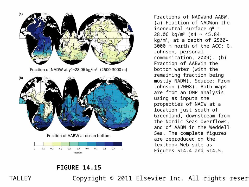
FIGURE 14.15

TALLEY

Fractions of NADWand AABW. (a) Fraction of NADWon the isoneutral surface gN = 28.06 kg/m3 (s4 ~ 45.84 kg/m3, at a depth of 2500-3000 m north of the ACC; G. Johnson, personal communication, 2009). (b) Fraction of AABWin the bottom water (with the remaining fraction being mostly NADW). Source: From Johnson (2008). Both maps are from an OMP analysis using as inputs the properties of NADW at a location just south of Greenland, downstream from the Nordic Seas Overflows, and of AABW in the Weddell Sea. The complete figures are reproduced on the textbook Web site as Figures S14.4 and S14.5.


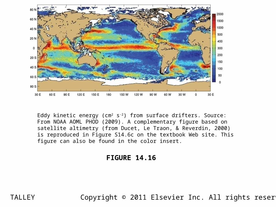
FIGURE 14.16

TALLEY

Eddy kinetic energy (cm2 s-2) from surface drifters. Source: From NOAA AOML PHOD (2009). A complementary figure based on satellite altimetry (from Ducet, Le Traon, & Reverdin, 2000) is reproduced in Figure S14.6c on the textbook Web site. This figure can also be found in the color insert.


FIGURE 14.17

TALLEY

(a) Horizontal eddy diffusivity (m2/sec) at the sea surface (color) with mean velocity vectors, based on surface drifter observations. Source: From Zhurbas and Oh (2004). (b) Eddy diffusivity ellipses at 900 m based on subsurface float velocities. Colors indicate different scales (see figure headers). Source: From Davis (2005). The Atlantic surface map and Indian 900 m map from the same sources are reproduced in Chapter S14 (Figures S14.7 and S14.8) on the textbook Web site. Both Figures 14.7a and 14.7b can also be found in the color insert.


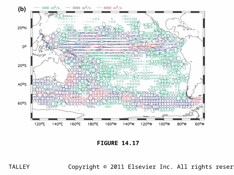
FIGURE 14.17


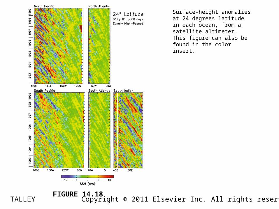
FIGURE 14.18TALLEY

Surface-height anomalies at 24 degrees latitude in each ocean, from a satellite altimeter. This figure can also be found in the color insert.


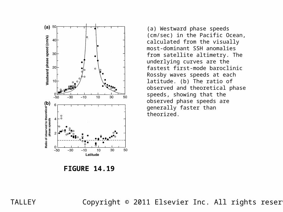
FIGURE 14.19

TALLEY

(a) Westward phase speeds (cm/sec) in the Pacific Ocean, calculated from the visually most-dominant SSH anomalies from satellite altimetry. The underlying curves are the fastest first-mode baroclinic Rossby waves speeds at each latitude. (b) The ratio of observed and theoretical phase speeds, showing that the observed phase speeds are generally faster than theorized.


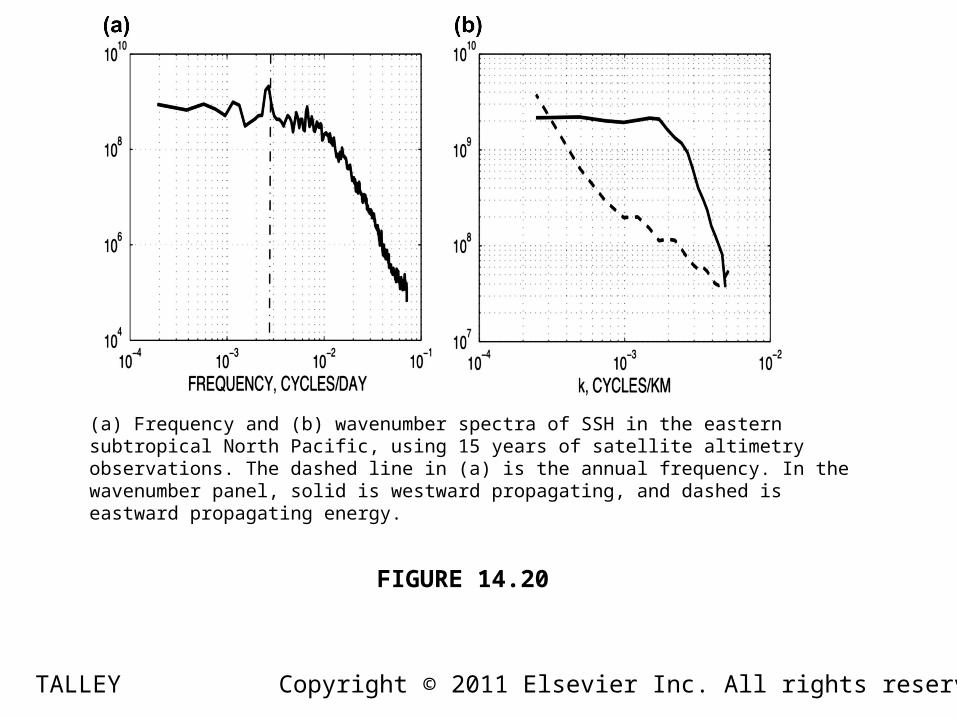
FIGURE 14.20

TALLEY

(a) Frequency and (b) wavenumber spectra of SSH in the eastern subtropical North Pacific, using 15 years of satellite altimetry observations. The dashed line in (a) is the annual frequency. In the wavenumber panel, solid is westward propagating, and dashed is eastward propagating energy.


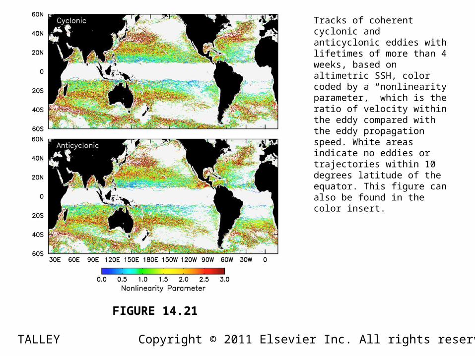
FIGURE 14.21

TALLEY

Tracks of coherent cyclonic and anticyclonic eddies with lifetimes of more than 4 weeks, based on altimetric SSH, color coded by a “nonlinearity parameter,” which is the ratio of velocity within the eddy compared with the eddy propagation speed. White areas indicate no eddies or trajectories within 10 degrees latitude of the equator. This figure can also be found in the color insert.


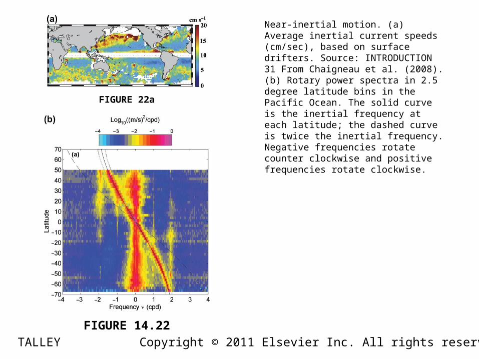
FIGURE 22a

FIGURE 14.22

TALLEY

Near-inertial motion. (a) Average inertial current speeds (cm/sec), based on surface drifters. Source: INTRODUCTION 31 From Chaigneau et al. (2008). (b) Rotary power spectra in 2.5 degree latitude bins in the Pacific Ocean. The solid curve is the inertial frequency at each latitude; the dashed curve is twice the inertial frequency. Negative frequencies rotate counter clockwise and positive frequencies rotate clockwise.


Documents

FIGURE 14.1 TALLEY Surface circulation schematic. This figure can also be found in the color insert. Copyright © 2011 Elsevier Inc. All rights reserved