Embed Size (px)
Citation preview

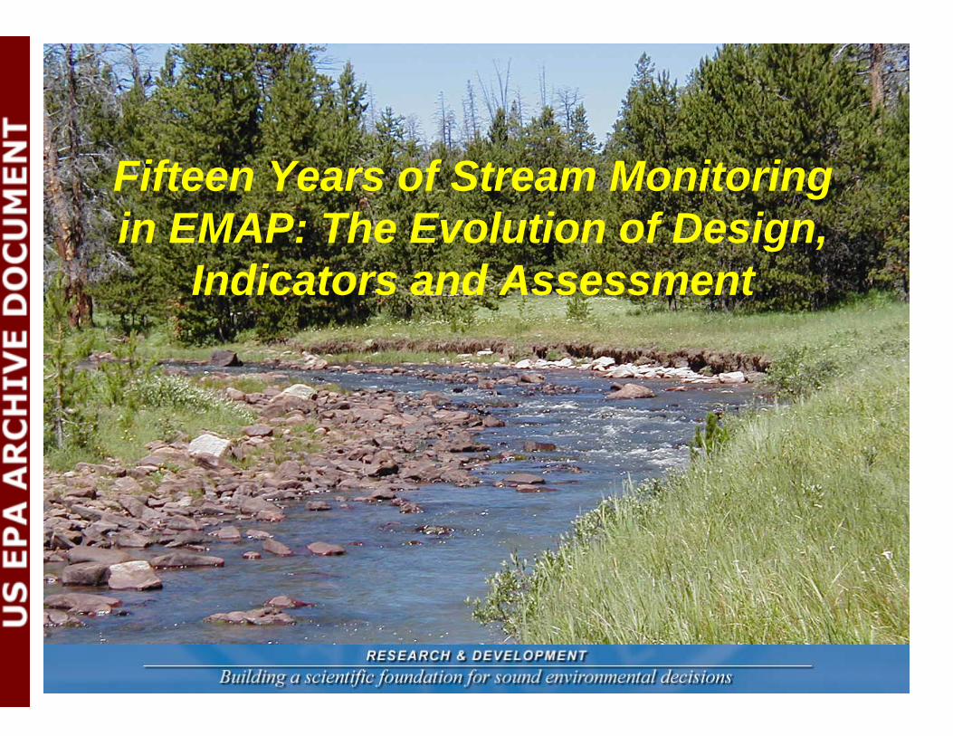
Fifteen Years of Stream Monitoring in EMAP: The Evolution of Design,
Indicators and Assessment
Contributors:Western Ecology Division, Corvallis:J.L. Stoddard.S.G. PaulsenD.V. PeckP.R. KaufmannA.R. OlsenJ. Van SickleS.A. PetersonP.L. RingoldOregon State University:A.T. HerlihyR.M. HughesT.R. WhittierMid-Continent Ecology Division, Duluth:B. H. HillEnvironmental Research Center, Cincinnati:D.J. KlemmJ.M. LazorchakPacific States Marine Fisheries Commission:D.P. LarsenU.S. Forest Service:F.H. McCormick
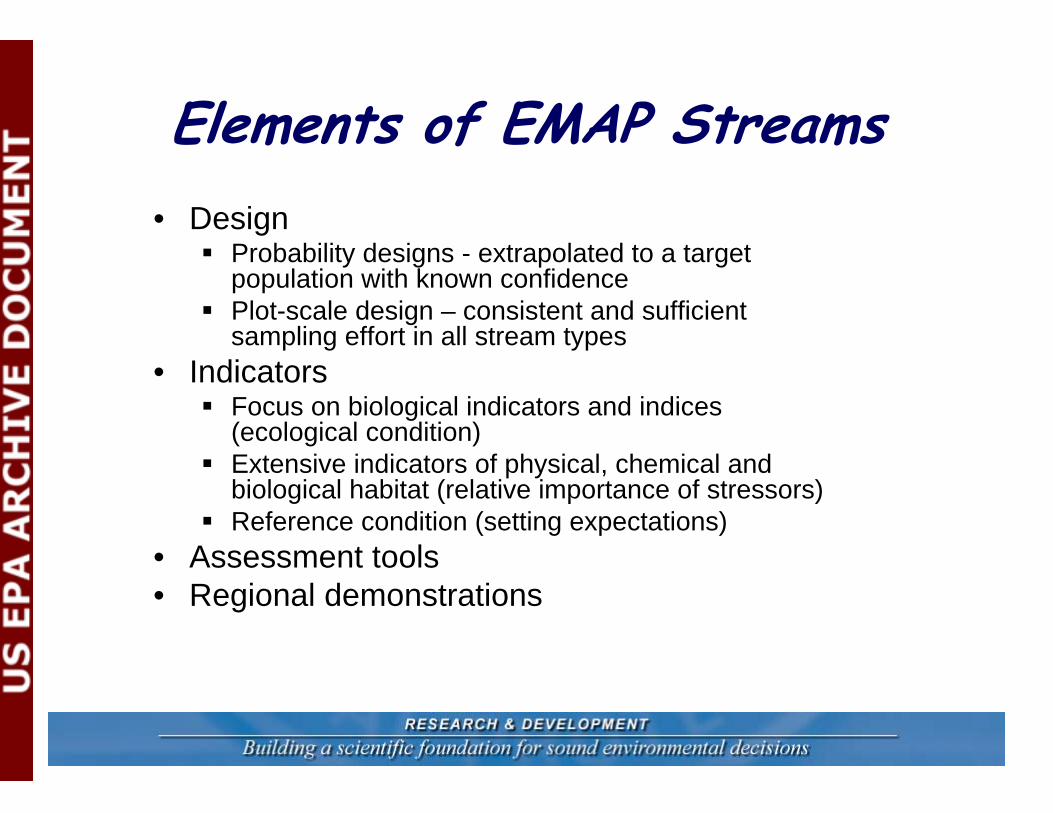
Elements of EMAP Streams • Design
Probability designs - extrapolated to a target population with known confidencePlot-scale design – consistent and sufficient sampling effort in all stream types
• IndicatorsFocus on biological indicators and indices (ecological condition)Extensive indicators of physical, chemical and biological habitat (relative importance of stressors)Reference condition (setting expectations)
• Assessment tools• Regional demonstrations
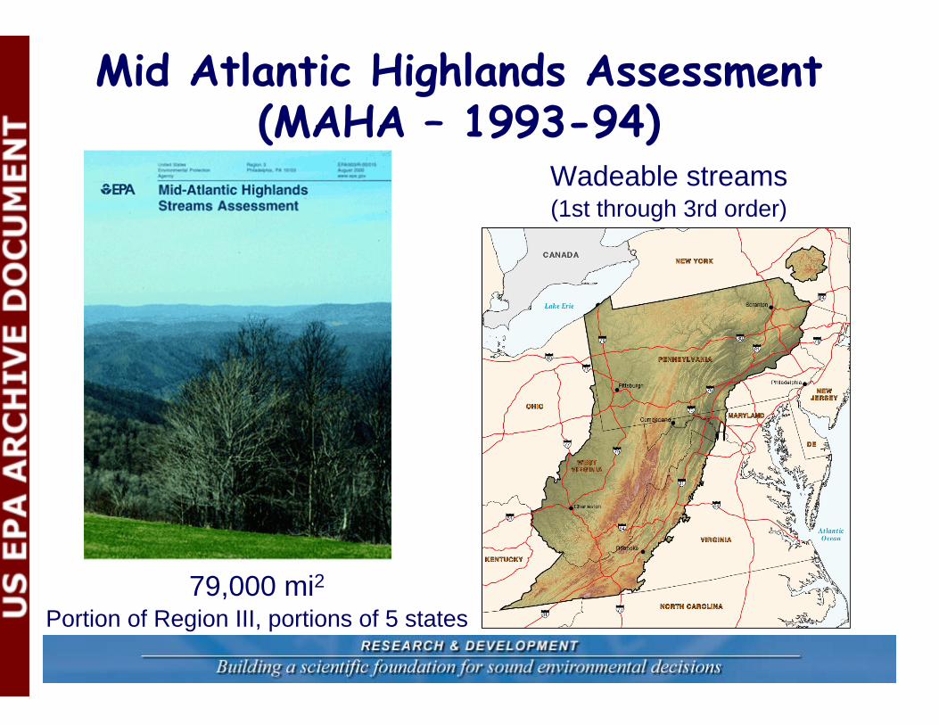
Mid Atlantic Highlands Assessment (MAHA – 1993-94)
Wadeable streams(1st through 3rd order)
79,000 mi2Portion of Region III, portions of 5 states
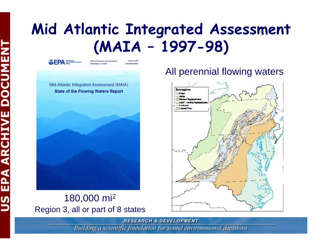
All perennial flowing waters
180,000 mi2Region 3, all or part of 8 states
Mid Atlantic Integrated Assessment (MAIA – 1997-98)
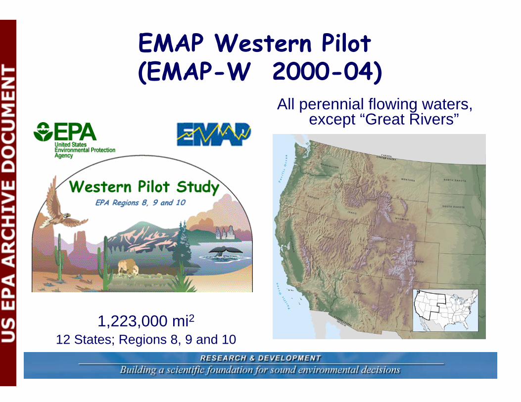
EMAP Western Pilot(EMAP-W 2000-04)
All perennial flowing waters, except “Great Rivers”
1,223,000 mi212 States; Regions 8, 9 and 10
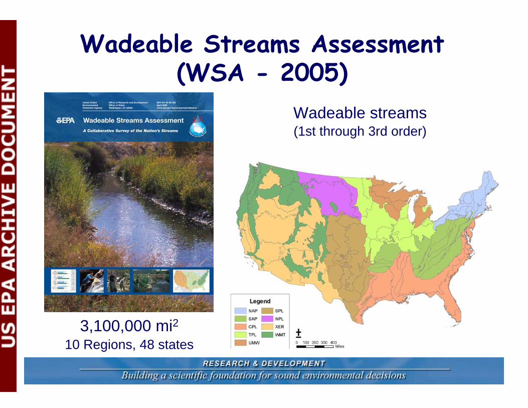
Wadeable Streams Assessment(WSA - 2005)
3,100,000 mi210 Regions, 48 states
Wadeable streams(1st through 3rd order)
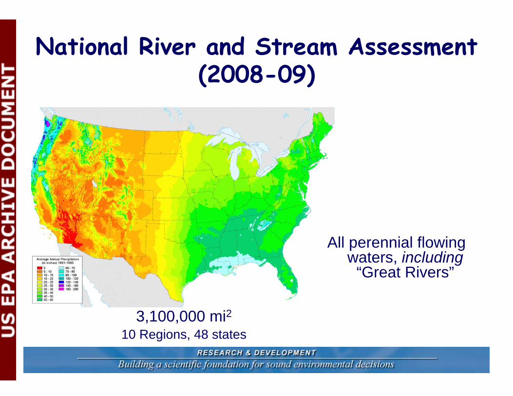
National River and Stream Assessment(2008-09)
3,100,000 mi210 Regions, 48 states
All perennial flowing waters, including
“Great Rivers”
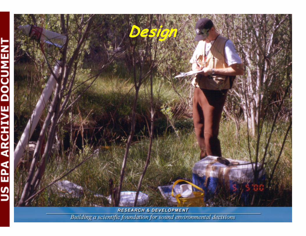
Design
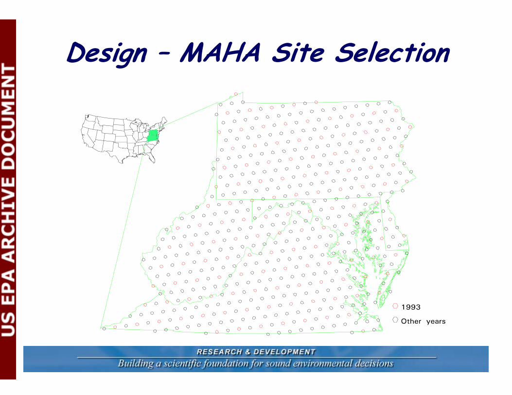
Design – MAHA Site Selection
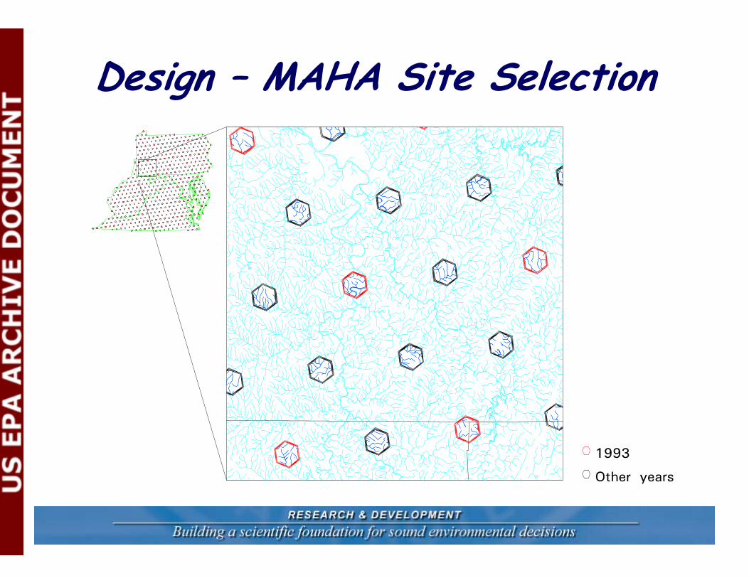
Design – MAHA Site Selection
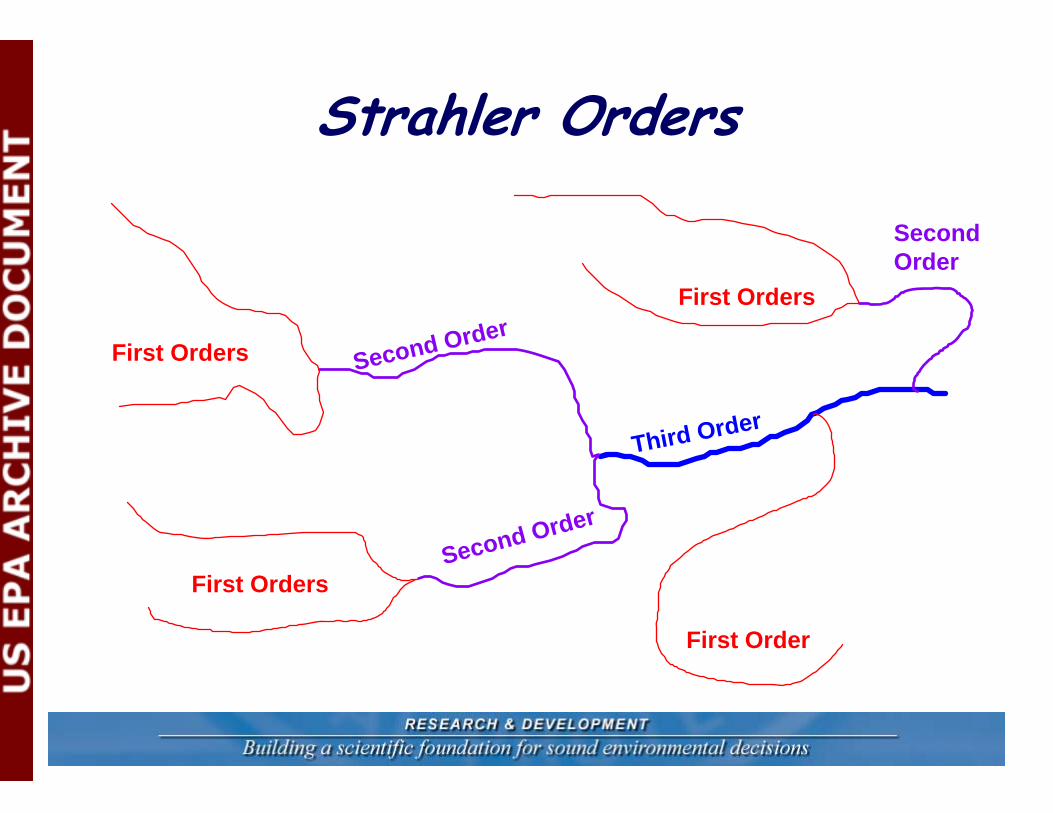
Strahler Orders
Third Order
First Orders
First Orders
First Order
First Orders
Second Order
Second Order
SecondOrder
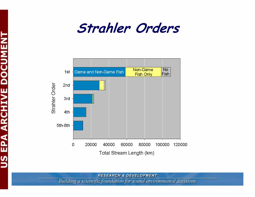
Strahler Orders
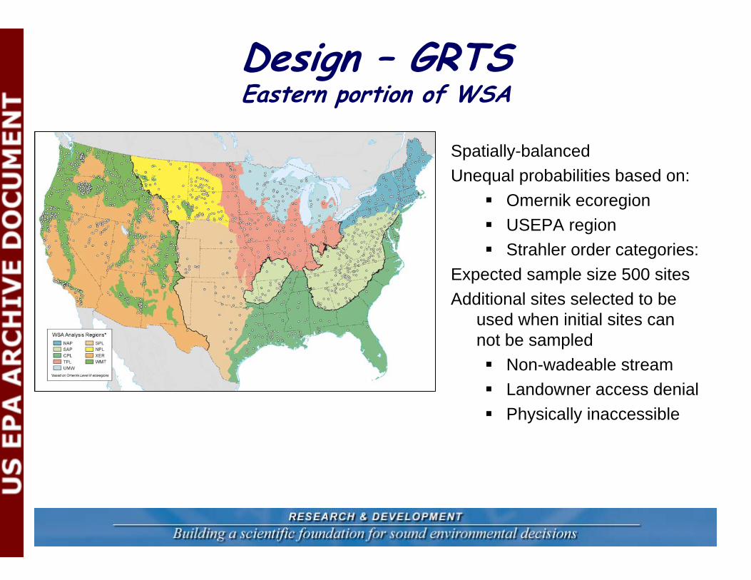
Spatially-balancedUnequal probabilities based on:
Omernik ecoregionUSEPA regionStrahler order categories:
Expected sample size 500 sitesAdditional sites selected to be
used when initial sites can not be sampled
Non-wadeable streamLandowner access denialPhysically inaccessible
Design – GRTSEastern portion of WSA
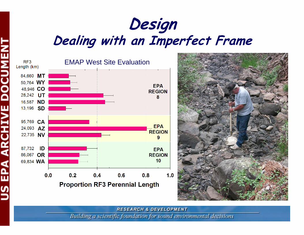
Design Dealing with an Imperfect Frame
EMAP West Site Evaluation
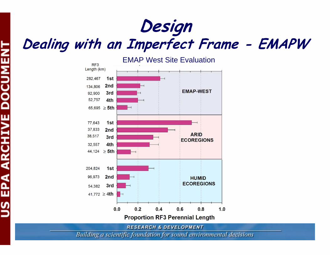
Design Dealing with an Imperfect Frame - EMAPW
EMAP West Site Evaluation
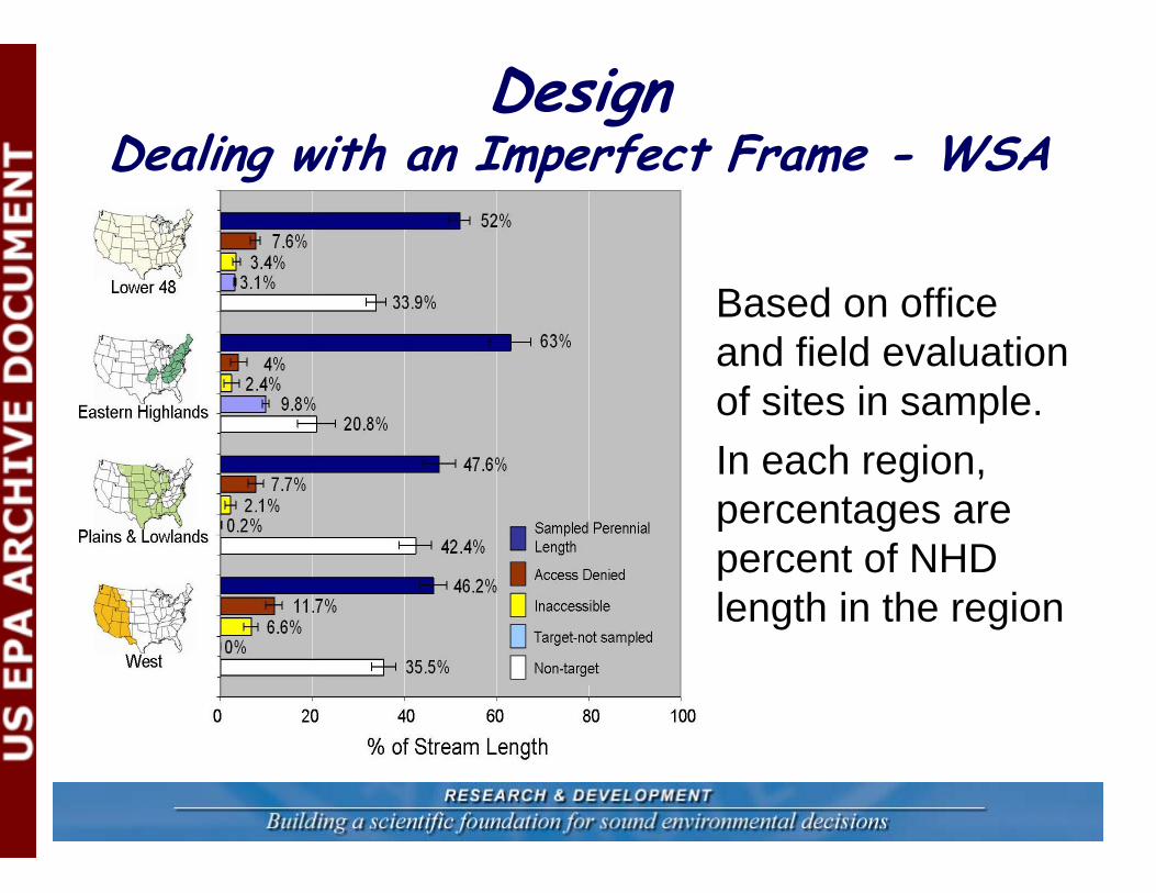
• Based on office and field evaluation of sites in sample.
• In each region, percentages are percent of NHD length in the region
Design Dealing with an Imperfect Frame - WSA
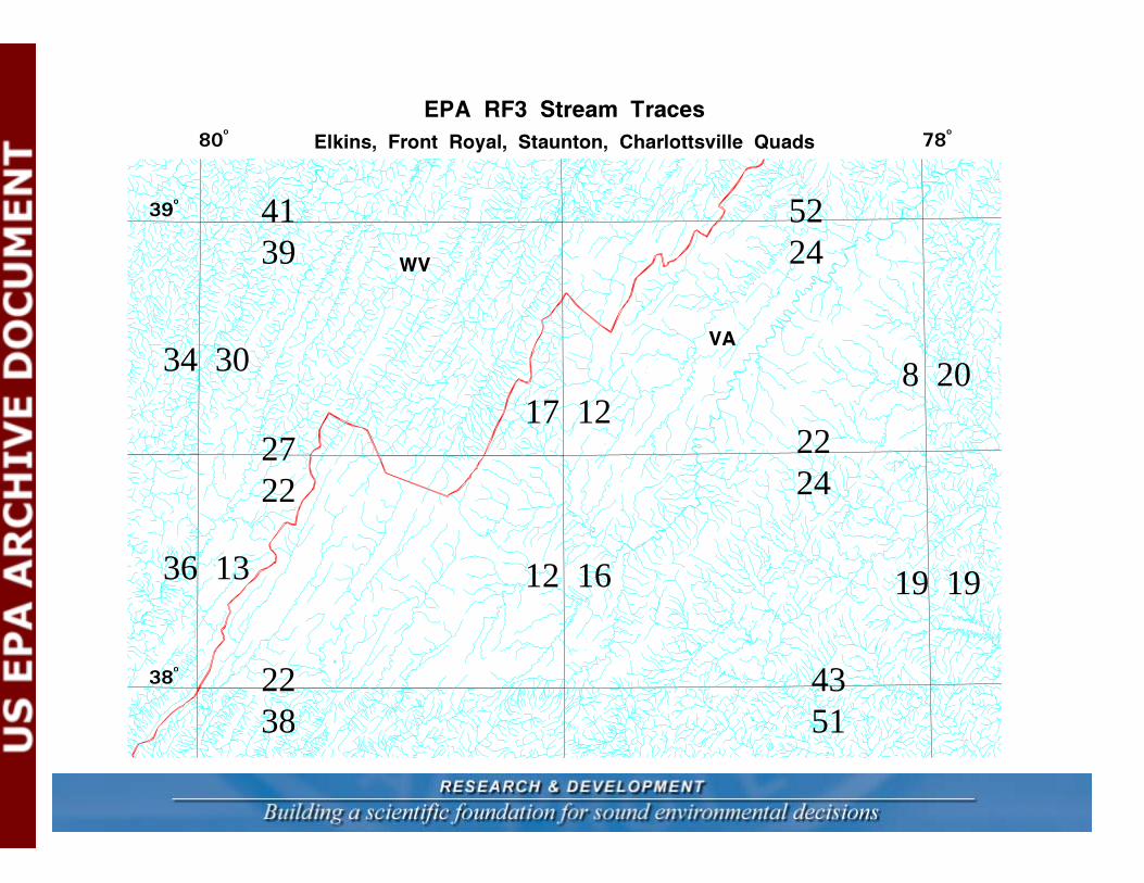
8 20
19 1912 1636 13
34 3017 12
5224
2224
4351
4139
2722
2238
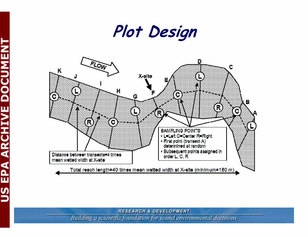
Plot Design
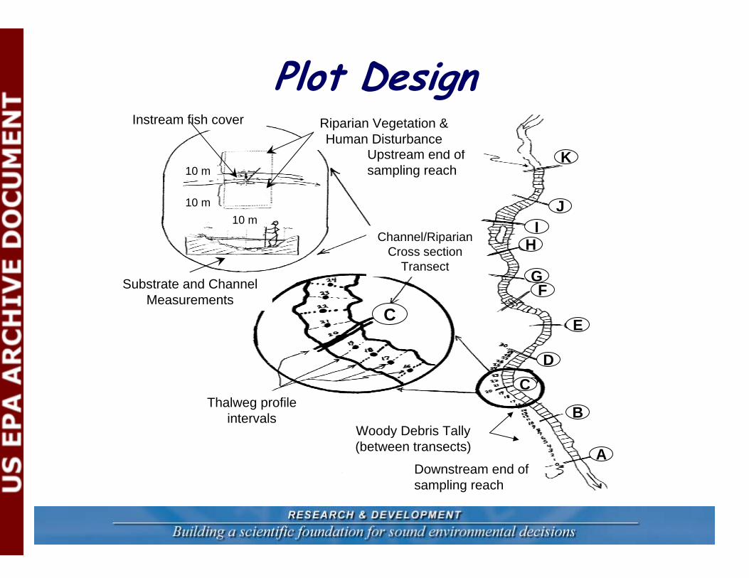
Plot Design
HI
J
K
E
DC
G
B
F
A
C
Thalweg profile intervals
Channel/Riparian Cross section
Transect
Upstream end of sampling reach
Downstream end of sampling reach
Riparian Vegetation & Human Disturbance
Substrate and Channel Measurements
Instream fish cover
10 m10 m
10 m
Woody Debris Tally(between transects)
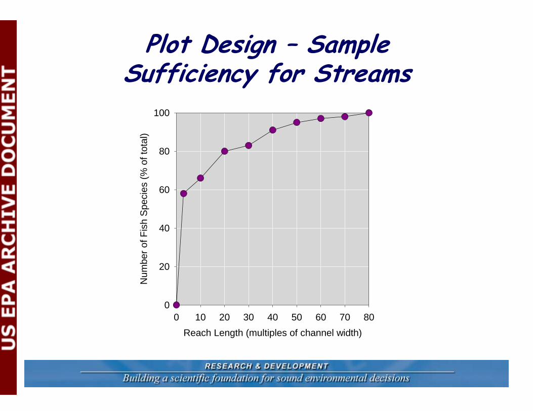
Plot Design – Sample Sufficiency for Streams
Reach Length (multiples of channel width)0 10 20 30 40 50 60 70 80
Num
ber o
f Fis
h S
peci
es (%
of t
otal
)
0
20
40
60
80
100
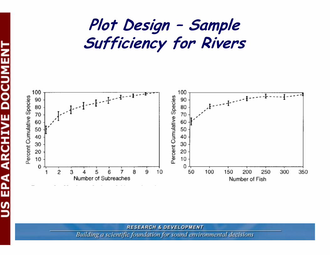
Plot Design – Sample Sufficiency for Rivers
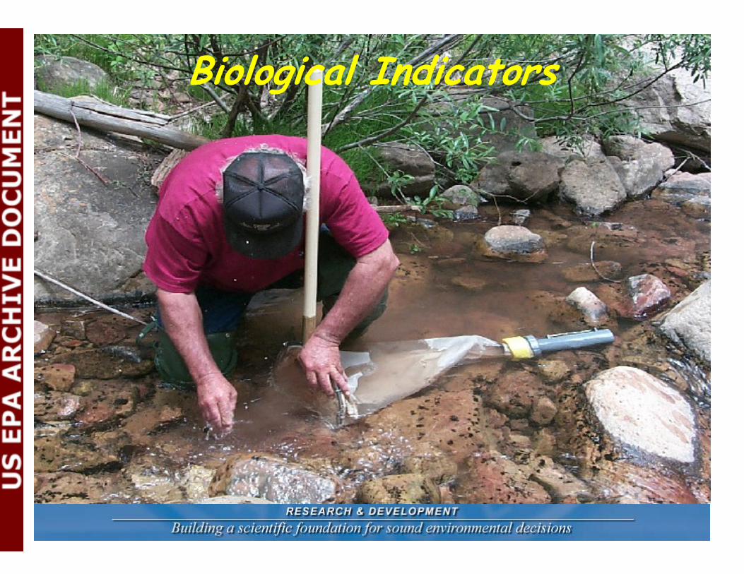
Biological Indicators
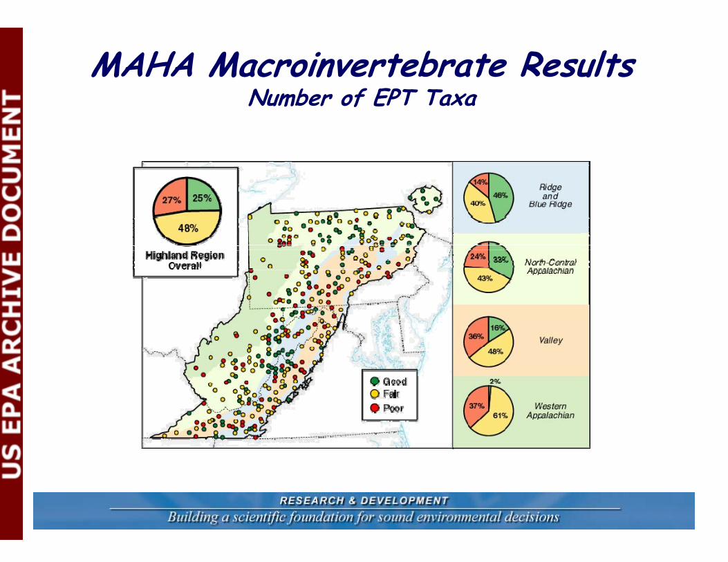
MAHA Macroinvertebrate ResultsNumber of EPT Taxa
MAHA Riffles
REFERENCE SO-SO TRASHED
EPT
Taxa
Ric
hnes
s
0
5
10
15
20
25
30MAHA Pools
REFERENCE SO-SO TRASHEDEP
T Ta
xa R
ichn
ess
0
5
10
15
20
25
30
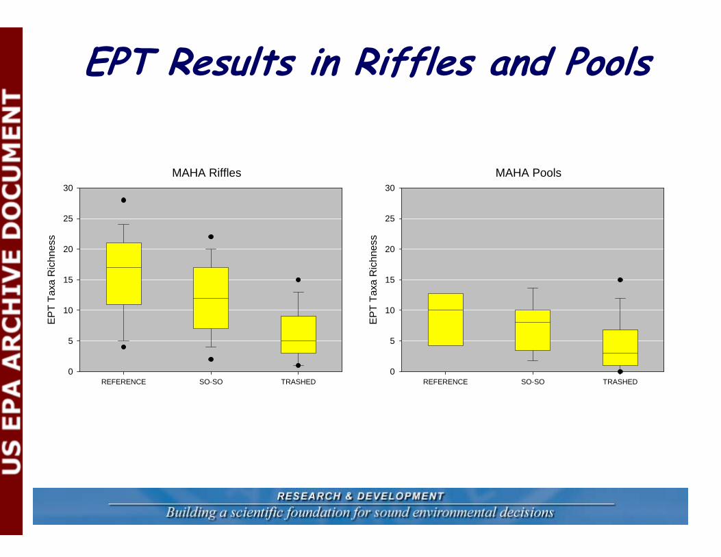
EPT Results in Riffles and Pools
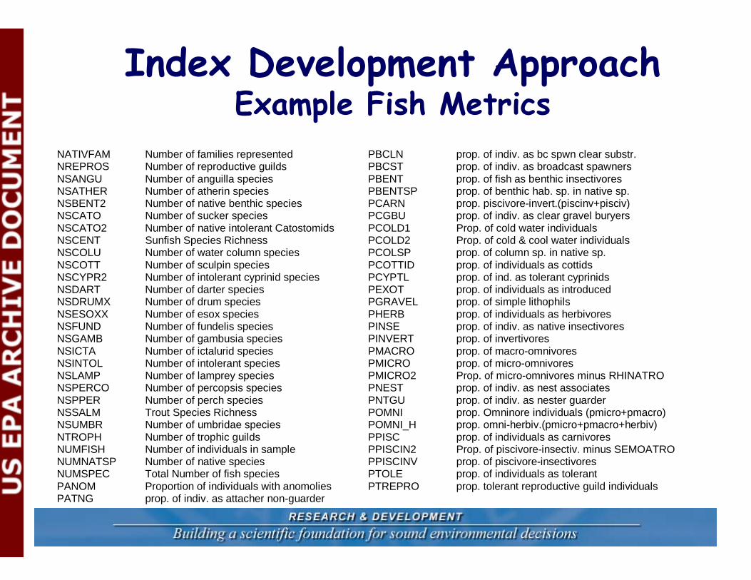
NATIVFAM Number of families represented NREPROS Number of reproductive guilds NSANGU Number of anguilla species NSATHER Number of atherin species NSBENT2 Number of native benthic species NSCATO Number of sucker species NSCATO2 Number of native intolerant Catostomids NSCENT Sunfish Species Richness NSCOLU Number of water column species NSCOTT Number of sculpin species NSCYPR2 Number of intolerant cyprinid species NSDART Number of darter species NSDRUMX Number of drum species NSESOXX Number of esox species NSFUND Number of fundelis species NSGAMB Number of gambusia species NSICTA Number of ictalurid species NSINTOL Number of intolerant species NSLAMP Number of lamprey species NSPERCO Number of percopsis species NSPPER Number of perch species NSSALM Trout Species Richness NSUMBR Number of umbridae species NTROPH Number of trophic guilds NUMFISH Number of individuals in sample NUMNATSP Number of native species NUMSPEC Total Number of fish species PANOM Proportion of individuals with anomolies PATNG prop. of indiv. as attacher non-guarder
PBCLN prop. of indiv. as bc spwn clear substr. PBCST prop. of indiv. as broadcast spawners PBENT prop. of fish as benthic insectivores PBENTSP prop. of benthic hab. sp. in native sp. PCARN prop. piscivore-invert.(piscinv+pisciv) PCGBU prop. of indiv. as clear gravel buryers PCOLD1 Prop. of cold water individuals PCOLD2 Prop. of cold & cool water individuals PCOLSP prop. of column sp. in native sp. PCOTTID prop. of individuals as cottids PCYPTL prop. of ind. as tolerant cyprinids PEXOT prop. of individuals as introduced PGRAVEL prop. of simple lithophils PHERB prop. of individuals as herbivores PINSE prop. of indiv. as native insectivores PINVERT prop. of invertivores PMACRO prop. of macro-omnivores PMICRO prop. of micro-omnivores PMICRO2 Prop. of micro-omnivores minus RHINATRO PNEST prop. of indiv. as nest associates PNTGU prop. of indiv. as nester guarder POMNI prop. Omninore individuals (pmicro+pmacro) POMNI_H prop. omni-herbiv.(pmicro+pmacro+herbiv) PPISC prop. of individuals as carnivores PPISCIN2 Prop. of piscivore-insectiv. minus SEMOATROPPISCINV prop. of piscivore-insectivores PTOLE prop. of individuals as tolerant PTREPRO prop. tolerant reproductive guild individuals
Index Development ApproachExample Fish Metrics

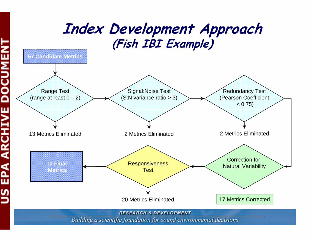
Index Development Approach(Fish IBI Example)
57 Candidate Metrics
Range Test(range at least 0 – 2)
Signal:Noise Test(S:N variance ratio > 3)
13 Metrics Eliminated 2 Metrics Eliminated
Redundancy Test(Pearson Coefficient
< 0.75)
2 Metrics Eliminated
Correction for Natural Variability
17 Metrics Corrected
ResponsivenessTest
10 FinalMetrics
20 Metrics Eliminated
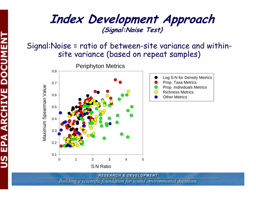
Signal:Noise = ratio of between-site variance and within-site variance (based on repeat samples)
Periphyton Metrics
S:N Ratio0 1 2 3 4 5
Max
imum
Spe
arm
an V
alue
0.1
0.2
0.3
0.4
0.5
0.6
0.7
0.8
Log S:N for Density MetricsProp. Taxa MetricsProp. Individuals MetricsRichness MetricsOther Metrics
Index Development Approach(Signal:Noise Test)
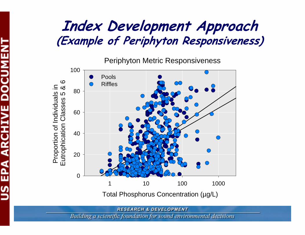
Index Development Approach(Example of Periphyton Responsiveness)
Periphyton Metric Responsiveness
Total Phosphorus Concentration (µg/L)1 10 100 1000
Pro
porti
on o
f Ind
ivid
uals
in
Eut
roph
icat
ion
Cla
sses
5 &
6
0
20
40
60
80
100PoolsRiffles
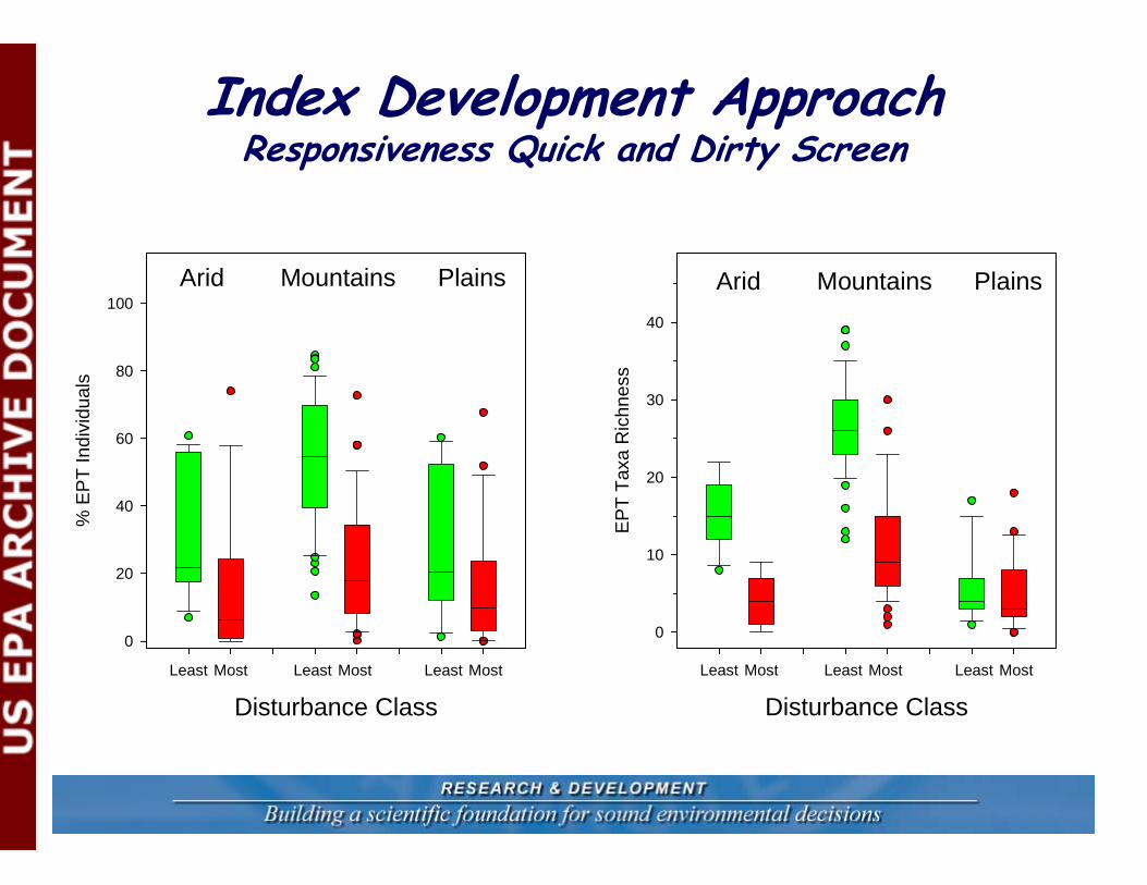
Index Development ApproachResponsiveness Quick and Dirty Screen
Disturbance ClassLeast Most Least Most Least Most
% E
PT
Indi
vidu
als
0
20
40
60
80
100 Arid Mountains Plains
Disturbance ClassLeast Most Least Most Least Most
EP
T Ta
xa R
ichn
ess
0
10
20
30
40
Arid Mountains Plains
Index Development Approach(Fish IBI Example)
57 Candidate Metrics
Range Test(range at least 0 – 2)
Signal:Noise Test(S:N variance ratio > 3)
13 Metrics Eliminated 2 Metrics Eliminated
Redundancy Test(Pearson Coefficient
< 0.75)
2 Metrics Eliminated
Correction for Natural Variability
17 Metrics Corrected
ResponsivenessTest
10 FinalMetrics
20 Metrics Eliminated
Metric Scoring
Mountains Plains XericRef Trash Ref Trash Ref Trash
% N
on-In
sect
Indi
vidu
als
0
20
40
60
80
100
0
10
0 - 10
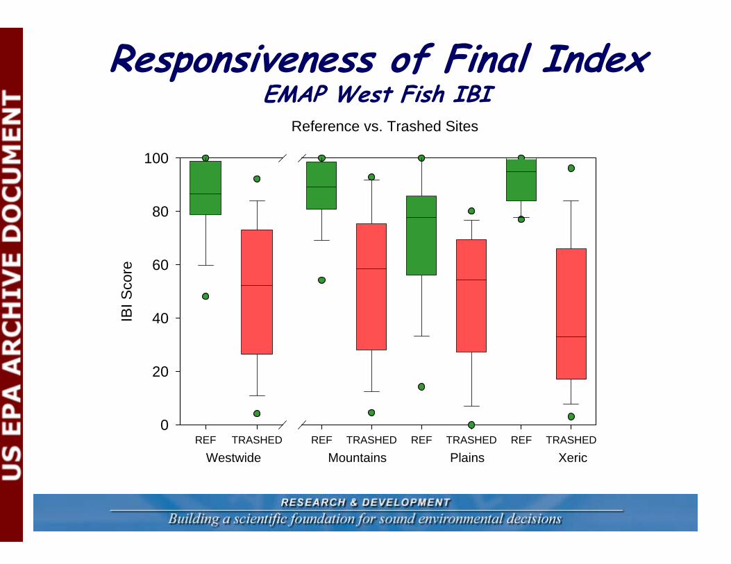
Reference vs. Trashed Sites
Westwide Mountains Plains XericREF TRASHED REF TRASHED REF TRASHED REF TRASHED
IBI S
core
0
20
40
60
80
100
Responsiveness of Final IndexEMAP West Fish IBI
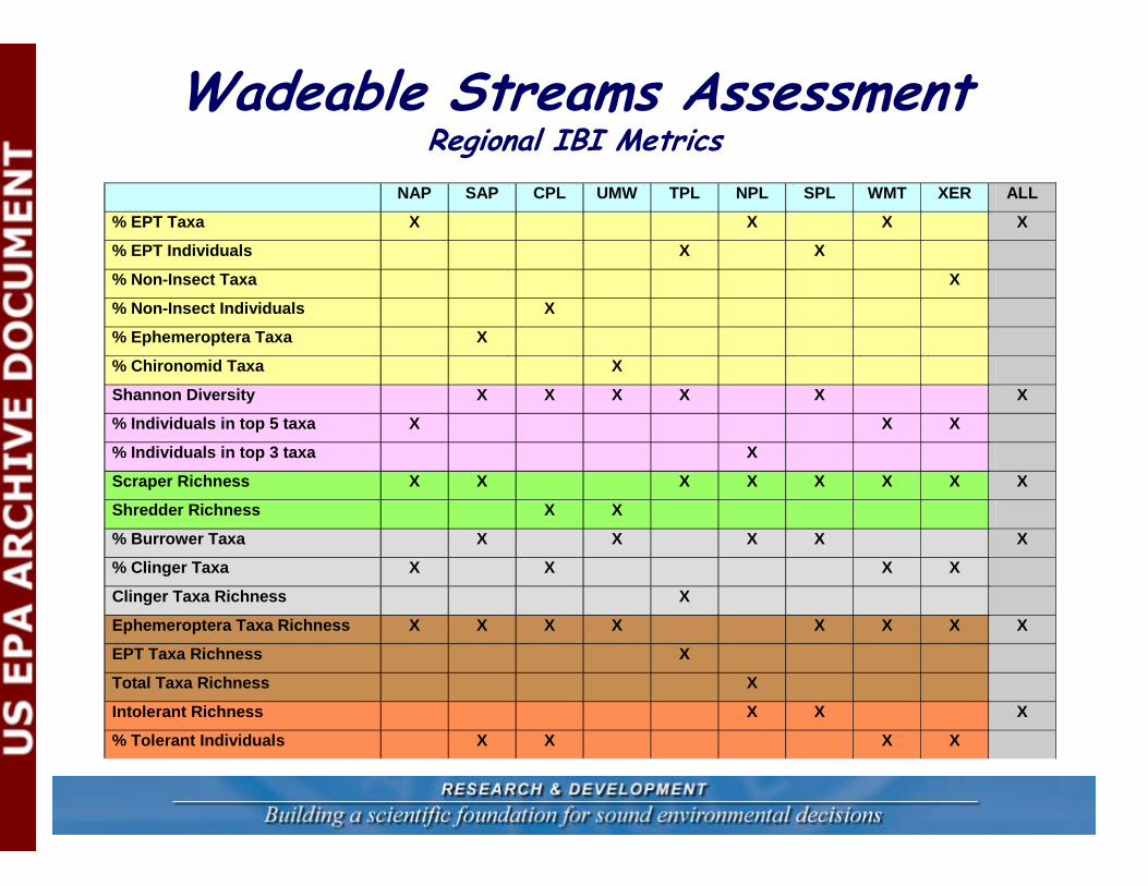
NAP SAP CPL UMW TPL NPL SPL WMT XER
% EPT Taxa X X X
% EPT Individuals X X
% Non-Insect Taxa X
% Non-Insect Individuals X
% Ephemeroptera Taxa X
% Chironomid Taxa X
Shannon Diversity X X X X X
% Individuals in top 5 taxa X X X
% Individuals in top 3 taxa X
Scraper Richness X X X X X X X
Shredder Richness X X
% Burrower Taxa X X X X
% Clinger Taxa X X X X
Clinger Taxa Richness X
Ephemeroptera Taxa Richness X X X X X X X
EPT Taxa Richness X
Total Taxa Richness X
Intolerant Richness X X
% Tolerant Individuals X X X X
NAP SAP CPL UMW TPL NPL SPL WMT XER ALL
% EPT Taxa X X X X
% EPT Individuals X X
% Non-Insect Taxa X
% Non-Insect Individuals X
% Ephemeroptera Taxa X
% Chironomid Taxa X
Shannon Diversity X X X X X X
% Individuals in top 5 taxa X X X
% Individuals in top 3 taxa X
Scraper Richness X X X X X X X X
Shredder Richness X X
% Burrower Taxa X X X X X
% Clinger Taxa X X X X
Clinger Taxa Richness X
Ephemeroptera Taxa Richness X X X X X X X X
EPT Taxa Richness X
Total Taxa Richness X
Intolerant Richness X X X
% Tolerant Individuals X X X X
Wadeable Streams AssessmentRegional IBI Metrics
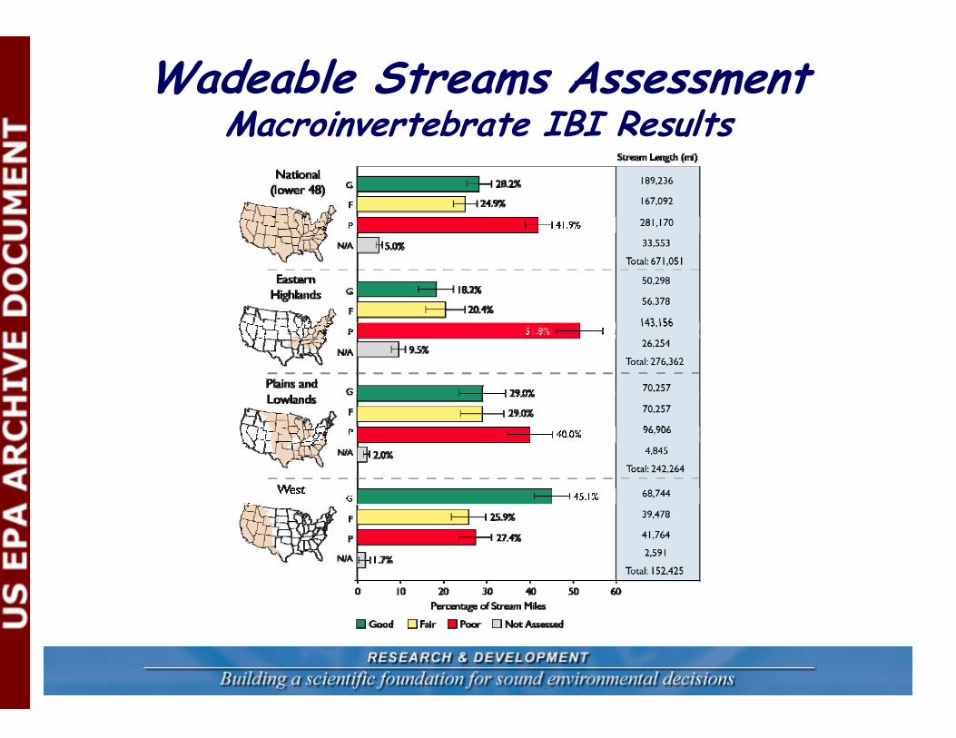
Wadeable Streams AssessmentMacroinvertebrate IBI Results
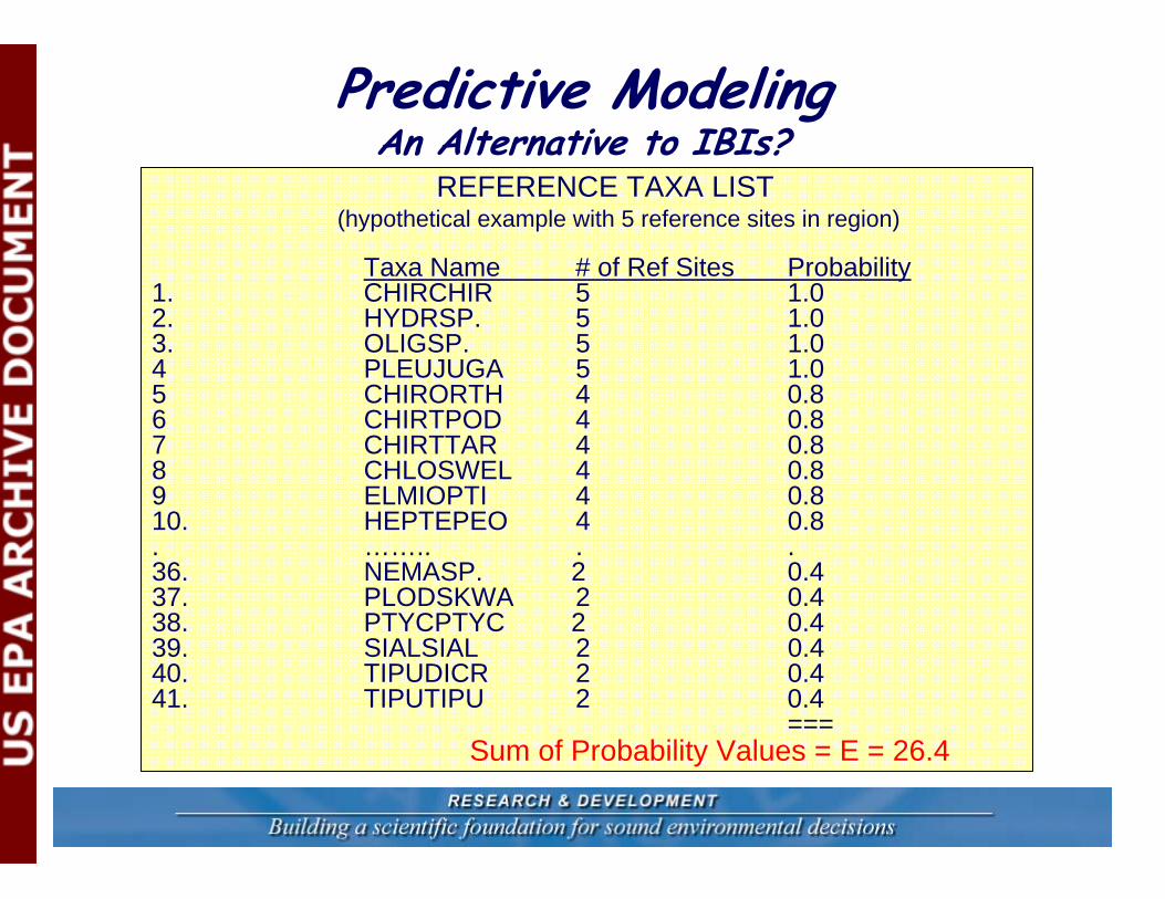
Predictive ModelingAn Alternative to IBIs?
REFERENCE TAXA LIST
Taxa Name # of Ref Sites Probability1. CHIRCHIR 5 1.02. HYDRSP. 5 1.03. OLIGSP. 5 1.04 PLEUJUGA 5 1.05 CHIRORTH 4 0.86 CHIRTPOD 4 0.87 CHIRTTAR 4 0.88 CHLOSWEL 4 0.89 ELMIOPTI 4 0.810. HEPTEPEO 4 0.8. …….. . .36. NEMASP. 2 0.437. PLODSKWA 2 0.438. PTYCPTYC 2 0.439. SIALSIAL 2 0.440. TIPUDICR 2 0.441. TIPUTIPU 2 0.4
===Sum of Probability Values = E = 26.4
(hypothetical example with 5 reference sites in region)
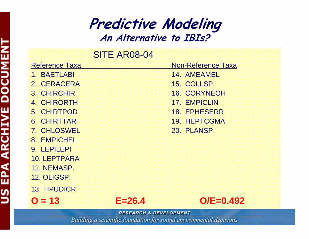
SITE AR08-04Reference Taxa Non-Reference Taxa1. BAETLABI 14. AMEAMEL2. CERACERA 15. COLLSP.3. CHIRCHIR 16. CORYNEOH4. CHIRORTH 17. EMPICLIN5. CHIRTPOD 18. EPHESERR6. CHIRTTAR 19. HEPTCGMA7. CHLOSWEL 20. PLANSP.8. EMPICHEL 9. LEPILEPI 10. LEPTPARA 11. NEMASP. 12. OLIGSP.
13. TIPUDICR
O = 13 E=26.4 O/E=0.492
Predictive ModelingAn Alternative to IBIs?
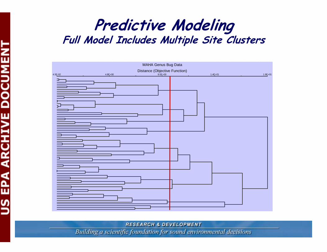
MAHA Genus Bug DataDistance (Objective Function)
4.5E-02 4.8E+00 9.5E+00 1.4E+01 1.9E+01
Predictive ModelingFull Model Includes Multiple Site Clusters
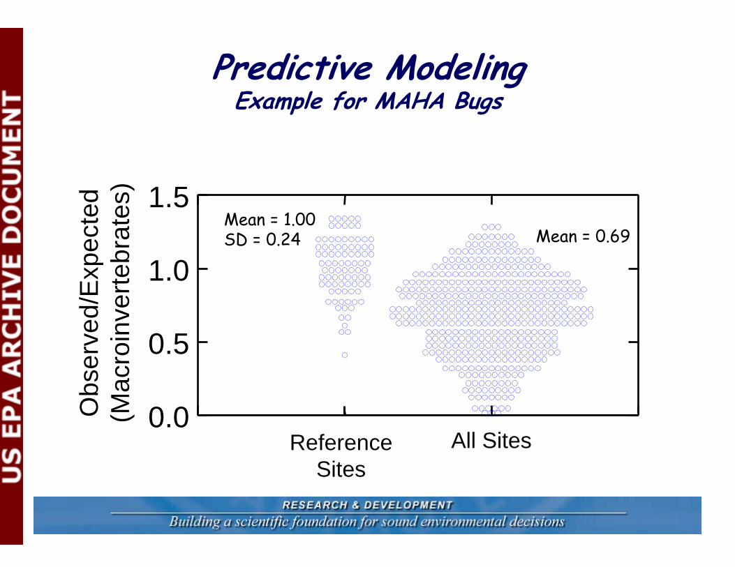
ReferenceSites
All Sites0.0
0.5
1.0
1.5
Obs
erve
d/E
xpec
ted
(Mac
roin
verte
brat
es)
Mean = 0.69Mean = 1.00SD = 0.24
Predictive ModelingExample for MAHA Bugs
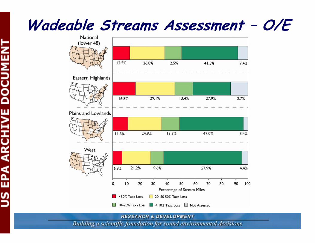
Wadeable Streams Assessment – O/E
0.0 0.5 1.0 1.5Observed/Expected
0.0
0.5
1.0
1.5
IBI S
core
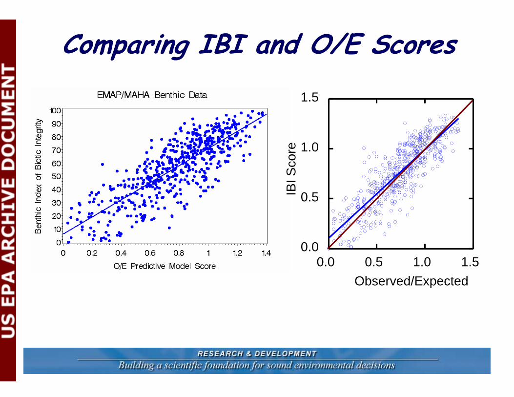
Comparing IBI and O/E Scores
Observed/Expected(3-Region Null Model)
0.0 0.2 0.4 0.6 0.8 1.0 1.2 1.4 1.6 1.8
Into
lera
nt T
axa
Ric
hnes
s
0
10
20
30
40
50
Mountains
Xeric
Plains
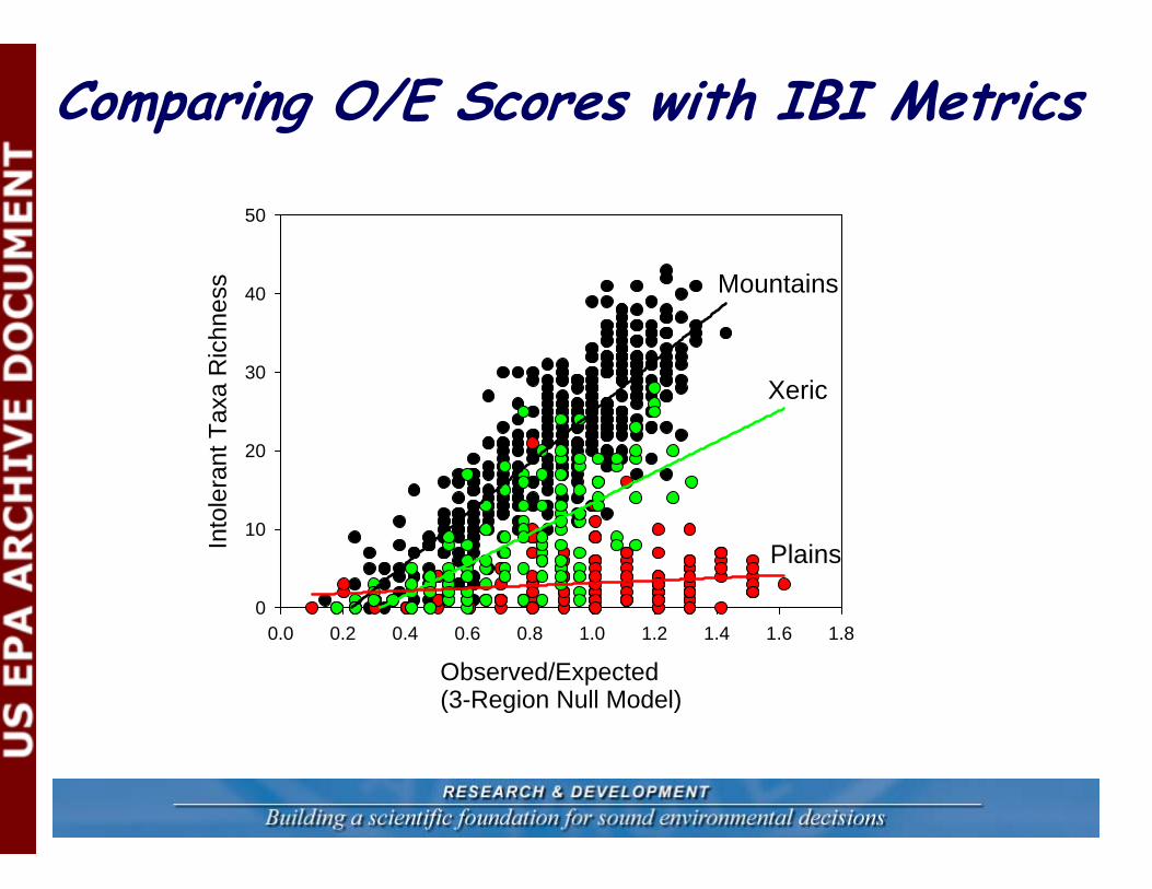
Comparing O/E Scores with IBI Metrics
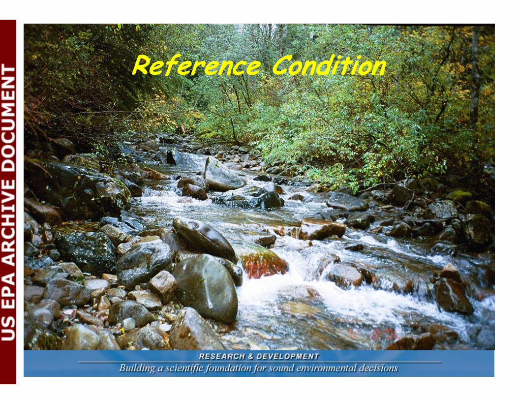
Reference Condition
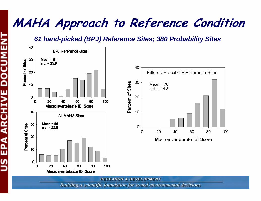
MAHA Approach to Reference Condition61 hand-picked (BPJ) Reference Sites; 380 Probability Sites
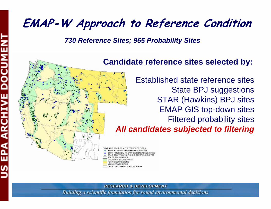
EMAP-W Approach to Reference Condition730 Reference Sites; 965 Probability Sites
Candidate reference sites selected by:
Established state reference sitesState BPJ suggestions
STAR (Hawkins) BPJ sitesEMAP GIS top-down sites
Filtered probability sitesAll candidates subjected to filtering
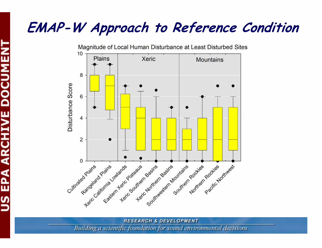
EMAP-W Approach to Reference Condition
Stressor Indicators
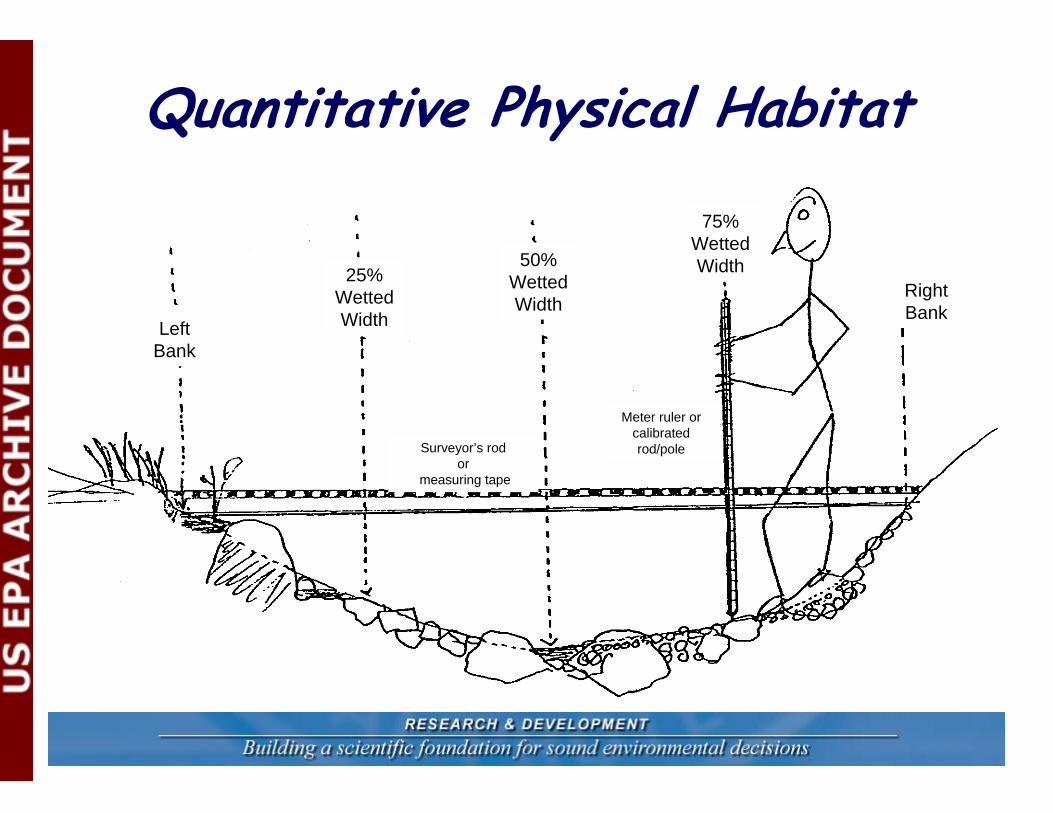
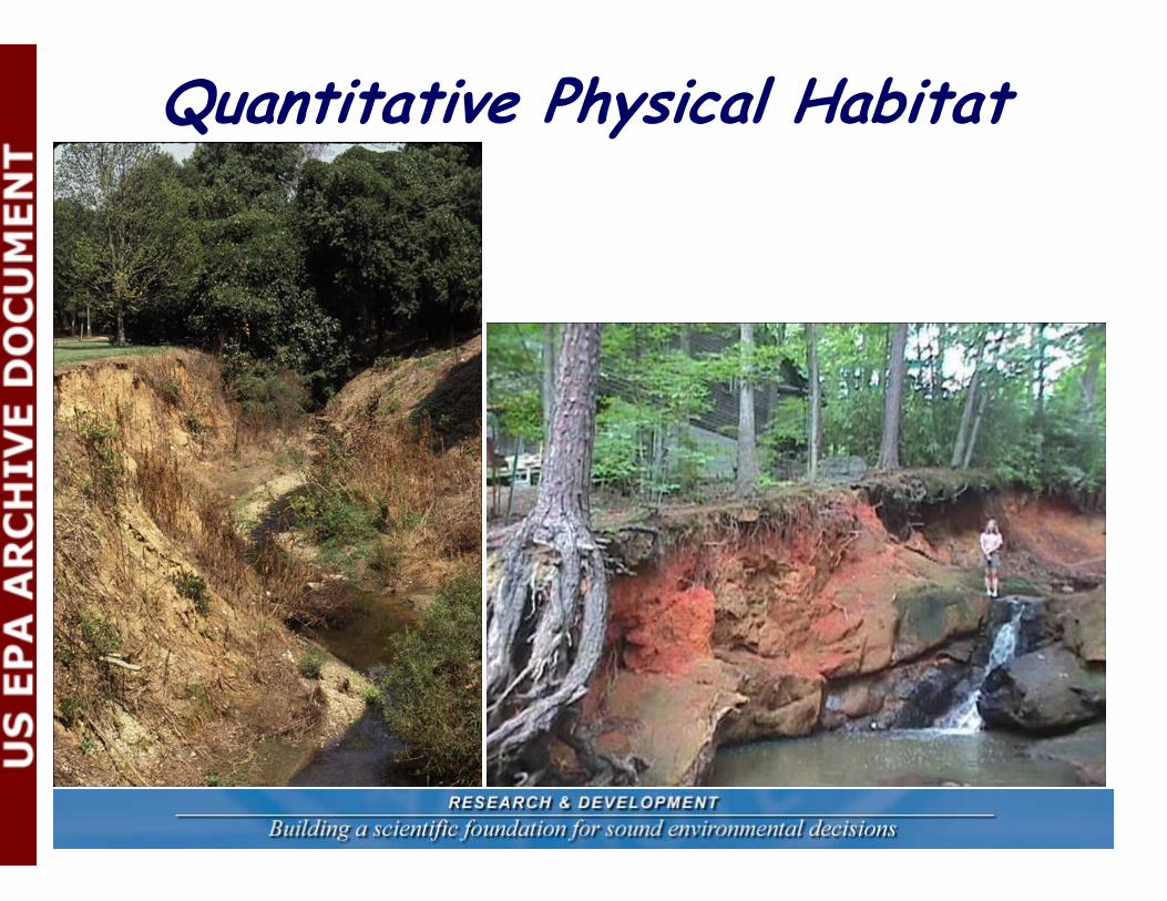
Quantitative Physical Habitat
Meter ruler or calibrated rod/poleSurveyor’s rod
ormeasuring tape
RightBank
25%Wetted Width
50%Wetted Width
75%Wetted Width
LeftBank
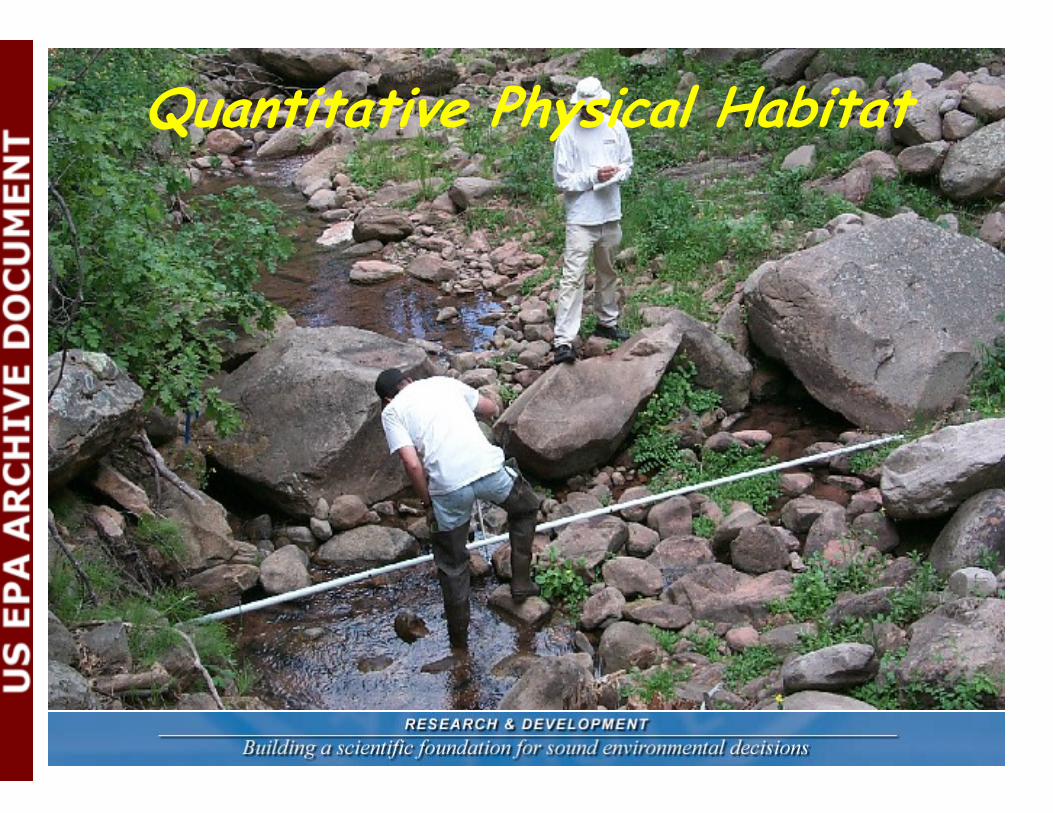
Quantitative Physical Habitat
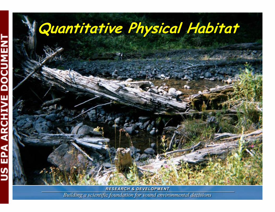
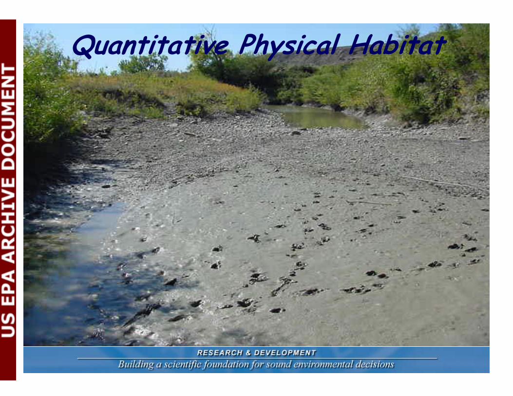
Quantitative Physical Habitat
Quantitative Physical Habitat
Quantitative Physical Habitat
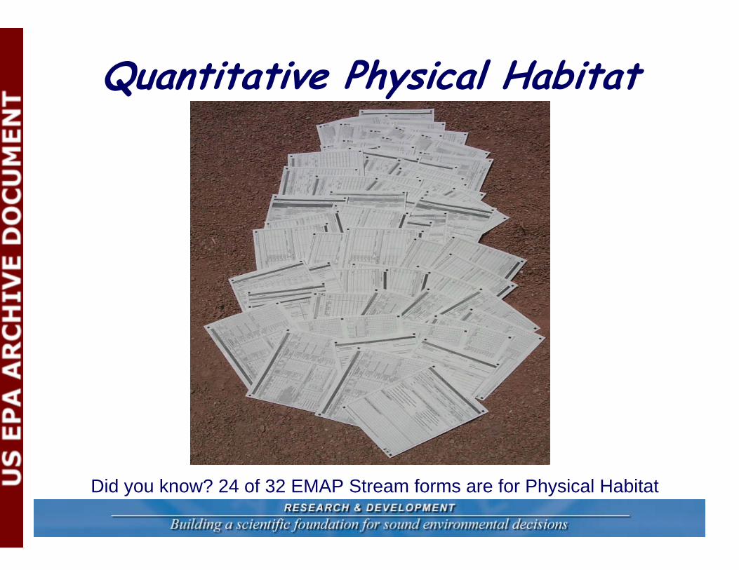
Quantitative Physical Habitat
Did you know? 24 of 32 EMAP Stream forms are for Physical Habitat
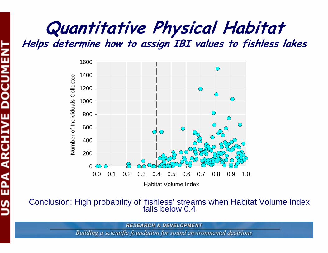
Habitat Volume Index
0.0 0.1 0.2 0.3 0.4 0.5 0.6 0.7 0.8 0.9 1.0
Num
ber o
f Ind
ivid
uals
Col
lect
ed
0
200
400
600
800
1000
1200
1400
1600
Conclusion: High probability of ‘fishless’ streams when Habitat Volume Index falls below 0.4
Quantitative Physical HabitatHelps determine how to assign IBI values to fishless lakes
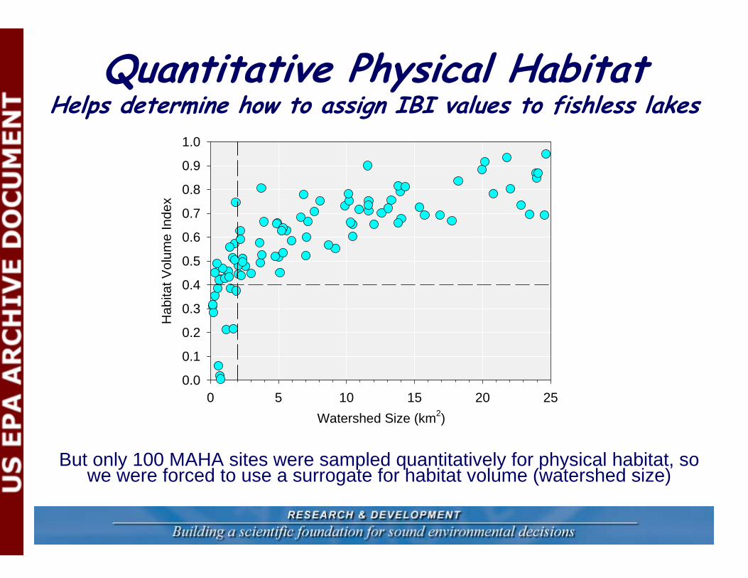
Watershed Size (km2)0 5 10 15 20 25
Hab
itat V
olum
e In
dex
0.0
0.1
0.2
0.3
0.4
0.5
0.6
0.7
0.8
0.9
1.0
But only 100 MAHA sites were sampled quantitatively for physical habitat, so we were forced to use a surrogate for habitat volume (watershed size)
Quantitative Physical HabitatHelps determine how to assign IBI values to fishless lakes
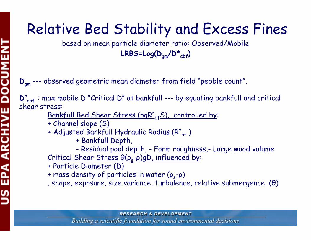
Relative Bed Stability and Excess Finesbased on mean particle diameter ratio: Observed/Mobile
LRBS=Log(Dgm/D*cbf)
Dgm --- observed geometric mean diameter from field “pebble count”.
D*cbf : max mobile D “Critical D” at bankfull --- by equating bankfull and critical
shear stress: Bankfull Bed Shear Stress (pgR*
bfS), controlled by:+ Channel slope (S)+ Adjusted Bankfull Hydraulic Radius (R*
bf )+ Bankfull Depth,- Residual pool depth, - Form roughness,- Large wood volume
Critical Shear Stress θ(ρs-ρ)gD, influenced by:+ Particle Diameter (D) + mass density of particles in water (ρs-ρ). shape, exposure, size variance, turbulence, relative submergence (θ)
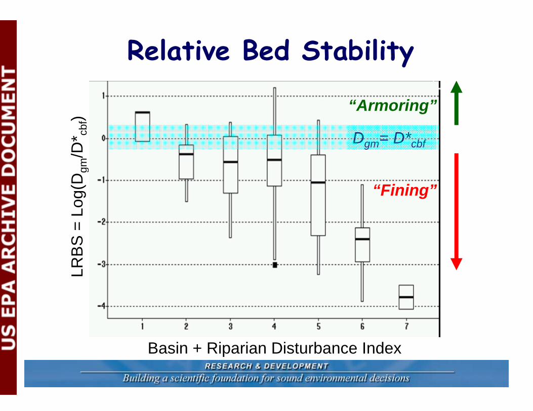
Relative Bed StabilityLR
BS
= L
og(D
gm/D
* cbf)
Basin + Riparian Disturbance Index
“Armoring”
Dgm= D*cbf
“Fining”
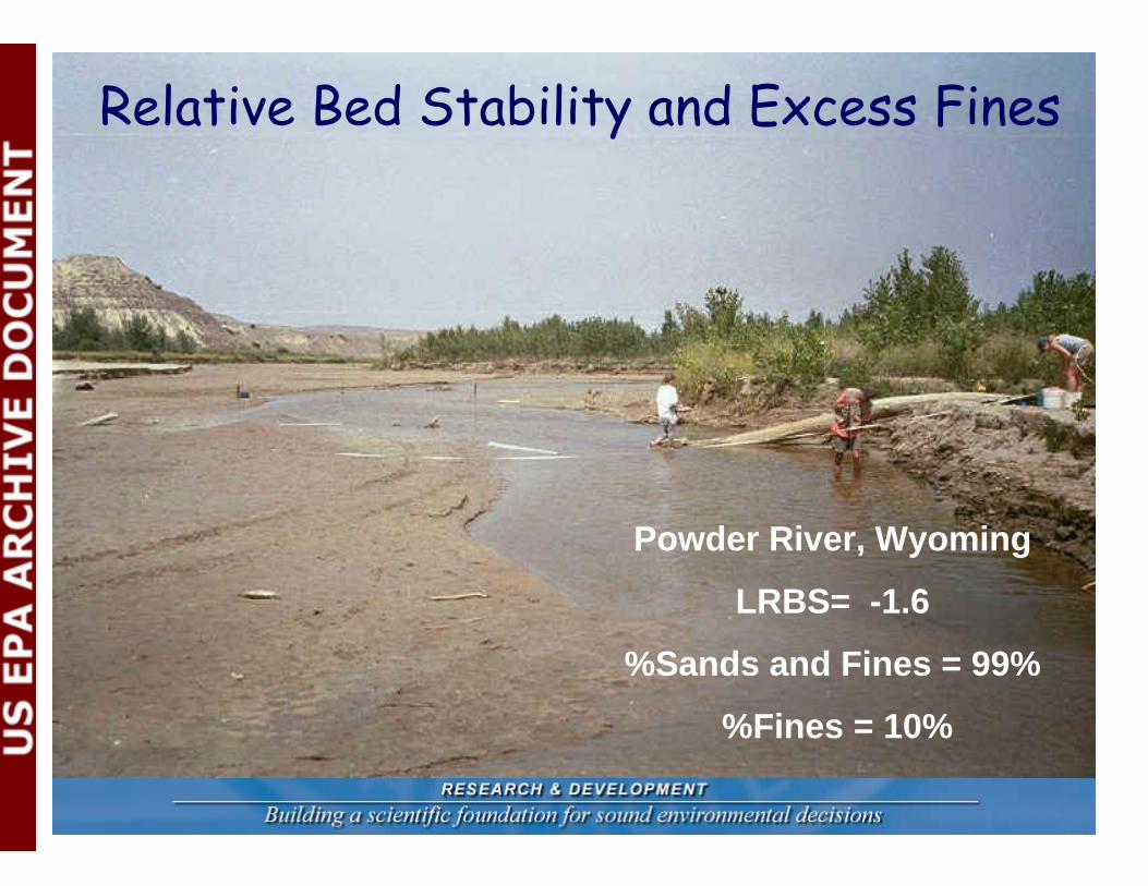
Relative Bed Stability and Excess Fines
Powder River, Wyoming
LRBS= -1.6
%Sands and Fines = 99%
%Fines = 10%
Relative Bed Stability and Excess Fines
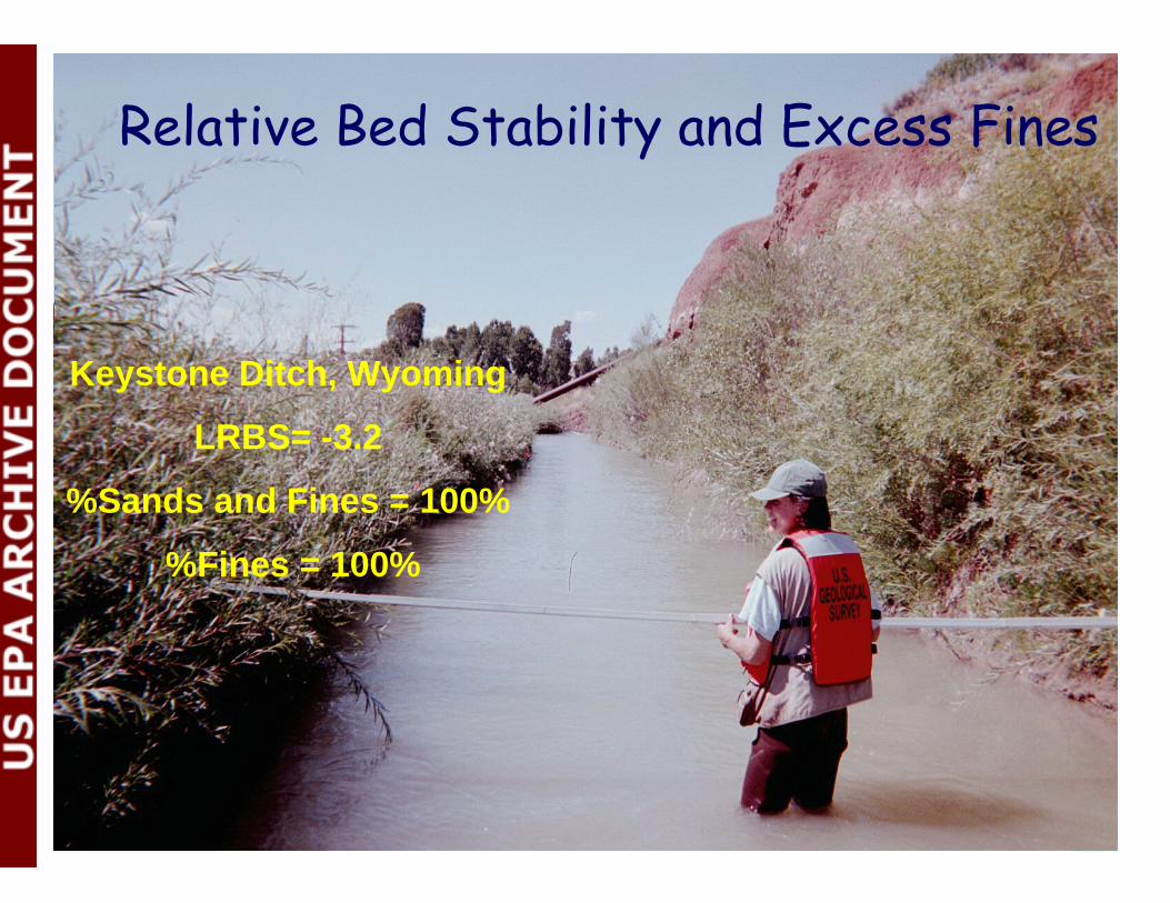
77
Keystone Ditch, Wyoming
LRBS= -3.2
%Sands and Fines = 100%
%Fines = 100%
Relative Bed Stability and Excess Fines
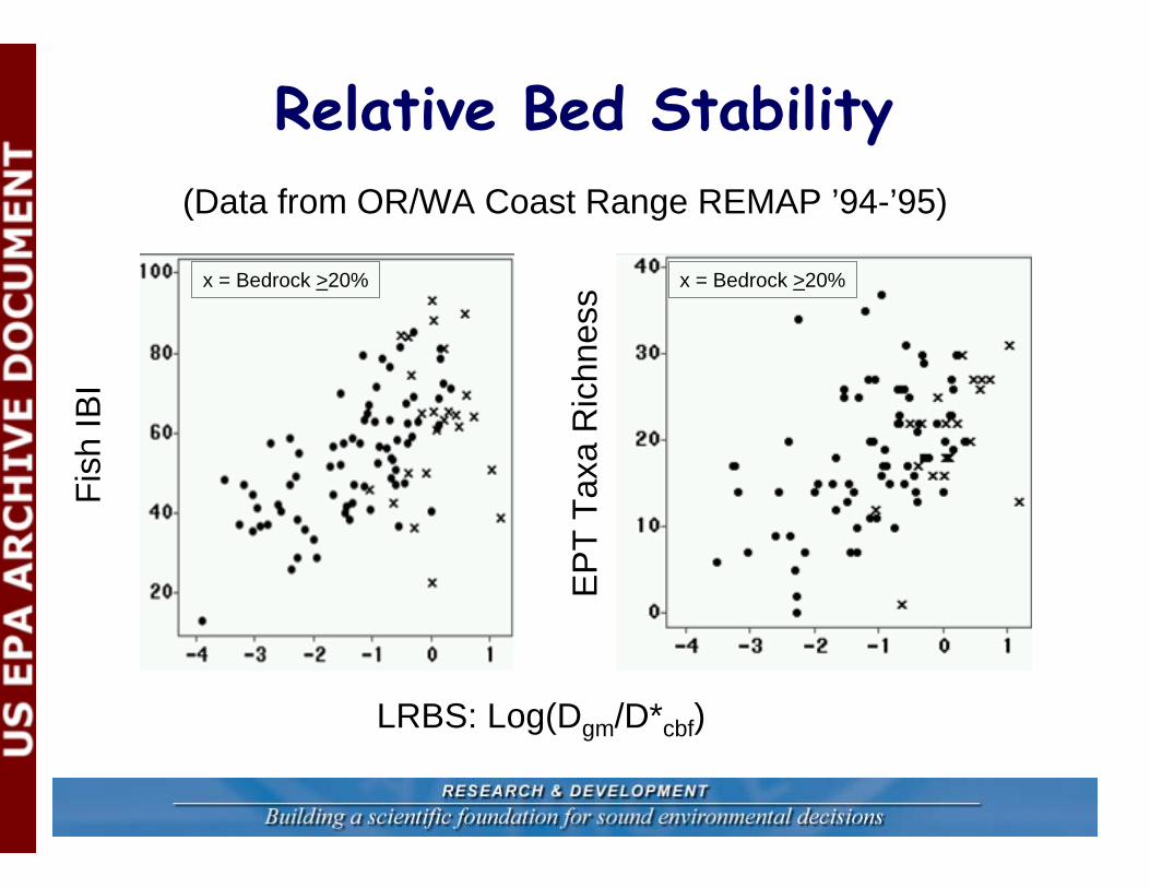
LRBS: Log(Dgm/D*cbf)
Fish
IBI
EP
T Ta
xa R
ichn
essx = Bedrock >20% x = Bedrock >20%
(Data from OR/WA Coast Range REMAP ’94-’95)
Relative Bed Stability
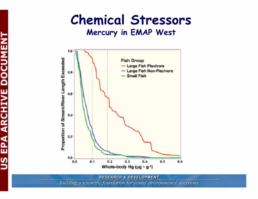
Chemical StressorsMercury in EMAP West
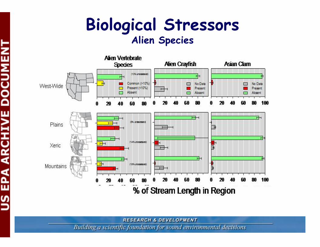
Biological StressorsAlien Species
Assessment
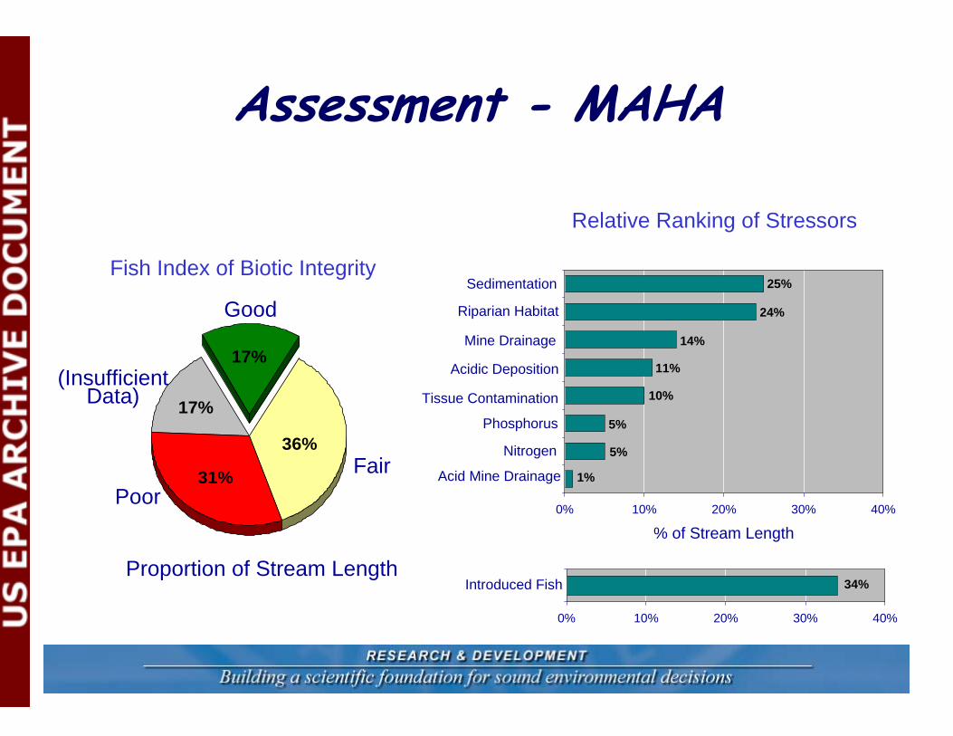
0% 10% 20% 30% 40%
Introduced Fish 34%
17%
17%
36%
31%
Proportion of Stream Length
(InsufficientData)
Good
FairPoor
Fish Index of Biotic Integrity
% of Stream Length0% 10% 20% 30% 40%
Riparian Habitat
Sedimentation
Mine Drainage
Acidic Deposition
Tissue Contamination
Phosphorus
Acid Mine Drainage
24%
25%
14%
11%
10%
5%
1%
Nitrogen
5%
Relative Ranking of Stressors
Assessment - MAHA
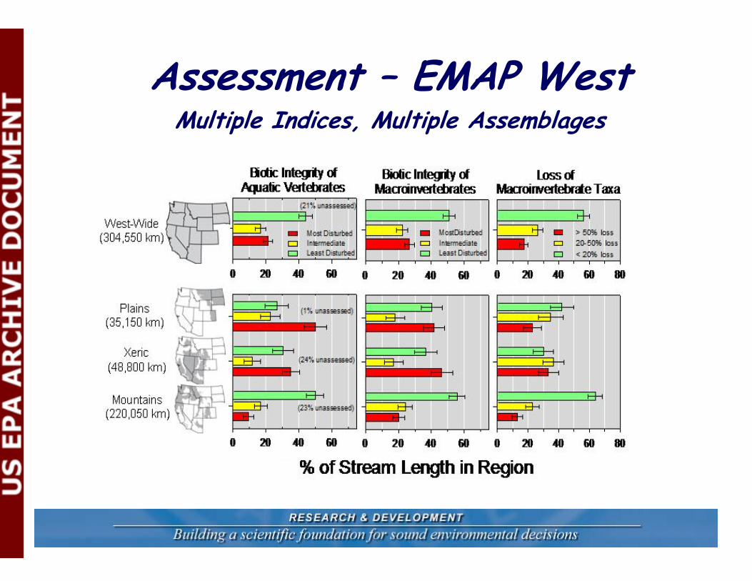
Assessment – EMAP WestMultiple Indices, Multiple Assemblages
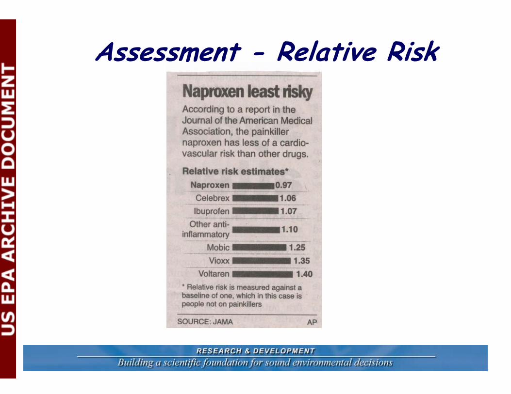
Assessment - Relative Risk
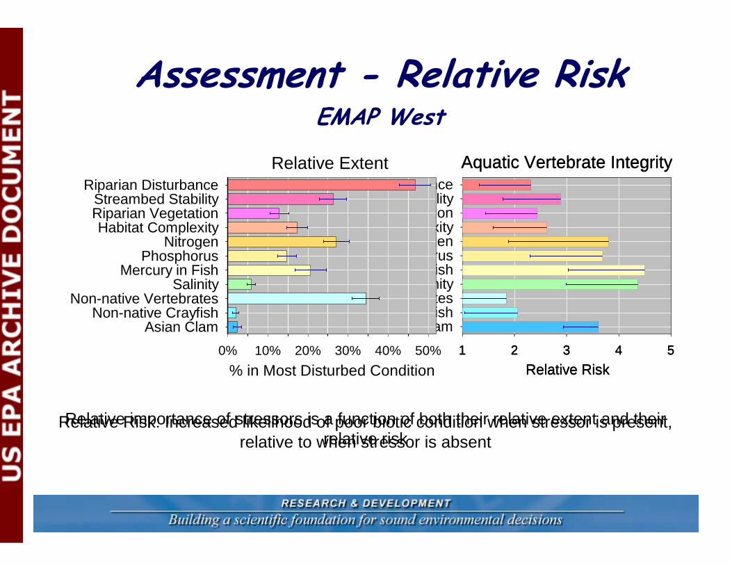
Assessment - Relative RiskEMAP West
Aquatic Vertebrate Integrity
Relative Risk1 2 3 4 5
Asian ClamNon-native Crayfish
Non-native VertebratesSalinity
Mercury in FishPhosphorus
NitrogenHabitat Complexity
Riparian VegetationStreambed Stability
Riparian Disturbance
Relative Risk: Increased likelihood of poor biotic condition when stressor is present,relative to when stressor is absent
Relative Extent
% in Most Disturbed Condition0% 10% 20% 30% 40% 50%
Asian ClamNon-native Crayfish
Non-native VertebratesSalinity
Mercury in FishPhosphorus
NitrogenHabitat Complexity
Riparian VegetationStreambed Stability
Riparian DisturbanceAquatic Vertebrate Integrity
Relative Risk1 2 3 4 5
Relative importance of stressors is a function of both their relative extent and their relative risk
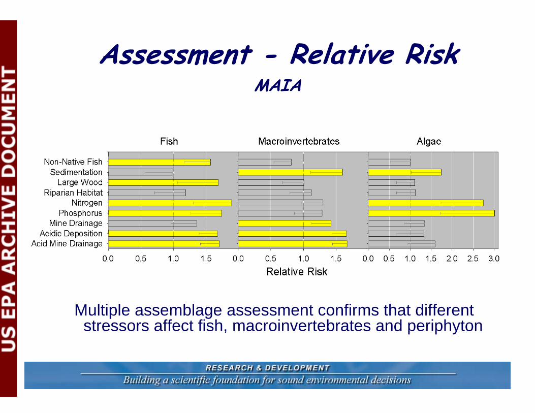
Assessment - Relative RiskMAIA
Multiple assemblage assessment confirms that different stressors affect fish, macroinvertebrates and periphyton
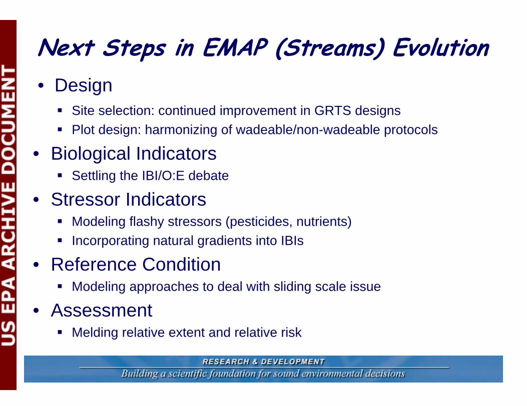
Next Steps in EMAP (Streams) Evolution
Site selection: continued improvement in GRTS designsPlot design: harmonizing of wadeable/non-wadeable protocols
• Biological IndicatorsSettling the IBI/O:E debate
• Stressor IndicatorsModeling flashy stressors (pesticides, nutrients)Incorporating natural gradients into IBIs
• Reference ConditionModeling approaches to deal with sliding scale issue
• AssessmentMelding relative extent and relative risk
• Design