Field theory and the Standard Model - CERN

Field theory and the Standard Model

W. Buchmüller and C. LüdelingDeutsches Elektronen-Synchrotron DESY, 22607 Hamburg, Germany

AbstractWe give a short introduction to the Standard Model and the underlying con-cepts of quantum field theory.

1 IntroductionIn these lectures we shall give a short introduction to the Standard Model of particle physics with empha-sis on the electroweak theory and the Higgs sector, and we shall also attempt to explain the underlyingconcepts of quantum field theory.

The Standard Model of particle physics has the following key features:

– As a theory of elementary particles, it incorporates relativity and quantum mechanics, and thereforeit is based on quantum field theory.

– Its predictive power rests on the regularization of divergent quantum corrections and the renormal-ization procedure which introduces scale-dependent ‘running couplings’.

– Electromagnetic, weak, strong and also gravitational interactions are all related to local symmetriesand described by Abelian and non-Abelian gauge theories.

– The masses of all particles are generated by two mechanisms: confinement and spontaneous sym-metry breaking.

In the following chapters we shall explain these points one by one. Finally, instead of a summary,we briefly recall the history of ‘The making of the Standard Model’ [1].

From the theoretical perspective, the Standard Model has a simple and elegant structure: it is achiral gauge theory. Spelling out the details reveals a rich phenomenology which can account for strongand electroweak interactions, confinement and spontaneous symmetry breaking, hadronic and leptonicflavour physics etc. [2, 3]. The study of all these aspects has kept theorists and experimenters busy forthree decades. Let us briefly consider these two sides of the Standard Model before we discuss the details.

1.1 Theoretical perspectiveThe Standard Model is a theory of fields with spins 0, 1

2 and 1. The fermions (matter fields) can bearranged in a big vector containing left-handed spinors only:

ΨTL =

(qL1, u

CR1, e

CR1, d

CR1, lL1, (n

CR1)︸︷︷︸

1st family

, qL2, . . .︸︷︷︸2nd

, . . . , (nCR3)︸︷︷︸3rd

), (1)

where the fields are the quarks and leptons, all in threefold family replication. The quarks come in tripletsof colour, i.e., they carry an index α, α = 1, 2, 3, which we suppressed in the above expression. Theleft-handed quarks and leptons come in doublets of weak isospin,

qαLi =

(uαLi

dαLi

)and lLi =

(νLieLi

),

where i is the family index i = 1, 2, 3. We have included a right-handed neutrino nR because there isevidence for neutrino masses from neutrino oscillation experiments.

1

The subscripts L and R denote left- and right-handed fields, respectively, which are eigenstatesof the chiral projection operators PL or PR. The superscript C indicates the charge conjugate field (theantiparticle). Note that the charge conjugate of a right-handed field is left-handed:

PLψL ≡1− γ5

2ψL = ψL , PLψ

CR = ψCR , PLψR = PLψ

CL = 0 , (2)

PRψR ≡1 + γ5

2ψR = ψR , PRψ

CL = ψCL , PRψL = PRψ

CR = 0 . (3)

So all fields in the big column vector of fermions have been chosen left-handed. Altogether there are48 chiral fermions. The fact that left- and right-handed fermions carry different weak isospin makes theStandard Model a chiral gauge theory. The threefold replication of quark-lepton families is one of thepuzzles whose explanation requires physics beyond the Standard Model [4].

The spin-1 particles are the gauge bosons associated with the fundamental interactions in theStandard Model,

GAµ , A = 1, . . . , 8 : the gluons of the strong interactions , (4)

W Iµ , I = 1, 2, 3 , Bµ : the W and B bosons of the electroweak interactions. (5)

These forces are gauge interactions, associated with the symmetry group

GSM = SU(3)C × SU(2)W × U(1)Y , (6)

where the subscripts C , W , and Y denote colour, weak isospin and hypercharge, respectively.

The gauge group acts on the fermions via the covariant derivative Dµ, which is an ordinary partialderivative, plus a big matrix Aµ built out of the gauge bosons and the generators of the gauge group:

DµΨL = (∂µ

+ gAµ) ΨL . (7)

From the covariant derivative we can also construct the field strength tensor,

Fµν = − ig

[Dµ, Dν ] , (8)

which is a matrix-valued object as well.

The last ingredient of the Standard Model is the Higgs field Φ, the only spin-0 field in the theory.It is a complex scalar field and a doublet of weak isospin. It couples left- and right-handed fermionstogether.

Written in terms of these fields, the Lagrangian of the theory is rather simple:

L = −1

2tr [FµνF

µν ] + ΨLiγµDµΨL + tr[(DµΦ)†DµΦ

]

+ µ2 Φ†Φ− 1

2λ(

Φ†Φ)2

+

(1

2ΨTLChΦΨL + h.c.

).

(9)

The matrix C in the last term is the charge conjugation matrix acting on the spinors, h is a matrix ofYukawa couplings. All coupling constants are dimensionless, in particular, there is no mass term for anyquark, lepton or vector boson. All masses are generated via the Higgs mechanism which gives a vacuumexpectation value to the Higgs field,

〈Φ〉 ≡ v = 174 GeV . (10)

The Higgs boson associated with the Higgs mechanism has not yet been found, but its discovery isgenerally expected at the LHC.

2

W. BUCHMÜLLER AND C. LÜDELING

2

1.2 Phenomenological aspectsThe Standard Model Lagrangian (9) has a rich structure which has led to different areas of research inparticle physics:

– The gauge group is composed of three subgroups with different properties:

– The SU(3) part leads to quantum chromodynamics, the theory of strong interactions [5].Here the most important phenomena are asymptotic freedom and confinement: The quarksand gluons appear as free particles only at very short distances, probed in deep-inelasticscattering, but are confined into mesons and baryons at large distances.

– The SU(2)× U(1) subgroup describes the electroweak sector of the Standard Model. It getsbroken down to the U(1)em subgroup of quantum electrodynamics by the Higgs mechanism,leading to massive W and Z bosons which are responsible for charged and neutral-currentweak interactions, respectively.

– The Yukawa interaction term can be split into different pieces for quarks and leptons:

1

2ΨTLChΦΨL = hu ij uRiqLjΦ + hd ij dRiqLjΦ + he ij eRilLjΦ + hn ijnRilLjΦ , (11)

where i, j = 1, 2, 3 label the families and Φa = εabΦ∗b . When the Higgs field develops a vacuum

expectation value 〈Φ〉 = v, the Yukawa interactions generate mass terms. The first two terms, massterms for up-type- and down-type-quarks, respectively, cannot be diagonalized simultaneously, andthis misalignment leads to the CKM matrix and flavour physics [6]. Similarly, the last two termsgive rise to lepton masses and neutrino mixings [7].

2 Quantization of fieldsIn this section we cover some basics of quantum field theory (QFT). For a more in-depth treatment, thereare many excellent books on QFT and its application in particle physics, such as Refs. [2, 3].

2.1 Why fields?2.1.1 Quantization in quantum mechanics

q(t)

q(t)

Fig. 1: Particle moving inone dimension

Quantum mechanics is obtained from classical mechanics by a methodcalled quantization. Consider, for example, a particle moving in one di-mension along a trajectory q(t), with velocity q(t) (see Fig. 1). Its mo-tion can be calculated in the Lagrangian or the Hamiltonian approach.The Lagrange function L(q, q) is a function of the position and the ve-locity of the particle, usually just the kinetic minus the potential energy.The equation of motion is obtained by requiring that the action, the timeintegral of the Lagrange function, be extremal, or, in other words, that itsvariation under arbitrary perturbations around the trajectory vanishes:

δS = δ

∫dtL (q(t), q(t)) = 0 . (12)

The Hamiltonian of the system, which corresponds to the total energy, depends on the coordinate q andits conjugate momentum p rather than q:

H(p, q) = pq − L (q, q) , p =∂L

∂q. (13)

3

FIELD THEORY AND THE STANDARD MODEL

3

To quantize the system, one replaces the coordinate and the momentum by operators q and pacting on some Hilbert space of states that we shall specify later. In the Heisenberg picture, the states aretime-independent and the operators change with time as

q(t) = eiHtq(0)e−iHt . (14)

Since p and q are now operators, they need not commute, and one postulates the commutation relation

[p(0), q(0)] = −i~ , (15)

where h = 2π~ is Planck’s constant. In the following we shall use units where ~ = c = 1. Thecommutator (15) leads to the uncertainty relation

∆q ·∆p ≥ 1

2. (16)

Note that on Schrödinger wave functions the operator q is just the coordinate itself and p is −i∂/∂q. Inthis way the commutation relation (15) is satisfied.

As an example example of a quantum mechanical system, consider the harmonic oscillator withthe Hamiltonian

H =1

2

(p2 + ω2q2

), (17)

which corresponds to a particle (with mass 1) moving in a quadratic potential with a strength character-ized by ω2. Classically, H is simply the sum of kinetic and potential energy. In the quantum system, wecan define new operators as linear combinations of p and q:

q =1√2ω

(a+ a†

), p = −i

√ω

2

(a− a†

), (18a)

i.e. , a =

√ω

2q + i

√1

2ωp , a† =

√ω

2q − i

√1

2ωp . (18b)

a and a† satisfy the commutation relations[a, a†

]= 1 . (19)

In terms of a and a† the Hamiltonian is given by

H =ω

2

(aa† + a†a

). (20)

Since Eqs. (18) are linear transformations, the new operators a and a† enjoy the same time evolution asq and p:

a(t) = eiHta(0)e−iHt = a(0)e−iωt , (21)

where the last equality follows from the commutator of a with the Hamiltonian,

[H, a] = −ωa ,[H, a†

]= ωa† . (22)

We can now construct the Hilbert space of states that the operators act on. We first notice that thecommutators (22) imply that a and a† decrease and increase the energy of a state, respectively. To seethis, suppose we have a state |E〉 with fixed energy, H|E〉 = E|E〉. Then

Ha|E〉 = (aH + [H, a])|E〉 = aE|E〉 − ωa|E〉 = (E − ω) a|E〉 . (23)

4


4

i.e., the energy of the state a|E〉 is (E−ω). In the same way one findsHa†|E〉 = (E + ω)|E〉. From theform of H we can also see that its eigenvalues must be positive. This suggests constructing the space ofstates starting from a lowest-energy state |0〉, the vacuum or no-particle state. This state needs to satisfy

a|0〉 = 0 , (24)

so its energy is ω/2. States with more ‘particles’, i.e., higher excitations, are obtained by successiveapplication of a†:

|n〉 =(a†)n|0〉 , with H|n〉 =

(n+

1

2

)ω|n〉 . (25)

2.1.2 Special relativity requires antiparticles

A1→B1+e−

∆Q=1

(t1 ,~x1)

(t2 ,~x2)

A2+e−→B2

∆Q=−1

Fig. 2: Electron moving from A1 to A2

So far, we have considered non-relativistic quantum me-chanics. A theory of elementary particles, however, hasto incorporate special relativity. It is very remarkable thatquantum mechanics together with special relativity impliesthe existence of antiparticles. To see this (following an ar-gument in Ref. [8]), consider two systems (e.g., atoms) A1

and A2 at positions ~x1 and ~x2. Assume that at time t1 atomA1 emits an electron and turns into B1. So the charge ofB1 is one unit higher than that of A1. At a later time t2 theelectron is absorbed by atom A2 which turns into B2 withcharge lower by one unit. This is illustrated in Fig. 2.

According to special relativity, we can also watch the system from a frame moving with relativevelocity ~v. One might now worry whether the process is still causal, i.e., whether the emission stillprecedes the absorption. In the boosted frame (with primed coordinates), one has

t′2 − t′1 = γ (t2 − t1) + γ~v (~x2 − ~x1) , γ =1√

1− ~v 2. (26)

Here t′2− t′1 must be positive for the process to remain causal. Since |~v| < 1, t′2− t′1 can only be negativefor spacelike distances, i.e., (t2 − t1)2 − (~x1 − ~x2)2 < 0. This, however, would mean that the electrontravelled faster than the speed of light, which is not possible according to special relativity. Hence, withinclassical physics, causality is not violated.

A2→B2+e+

∆Q=−1

(t′2 ,~x′2)

(t′1 ,~x′1)

A1+e+→B1

∆Q=1

Fig. 3: Positron moving from A2 to A1

This is where quantum mechanics comes in. The un-certainty relation leads to a ‘fuzzy’ light cone, which gives anon-negligible propagation probability for the electron evenfor slightly spacelike distances, as long as

(t2 − t1)2 − (~x1 − ~x2)2 & − ~2

m2. (27)

Does this mean causality is violated?

Fortunately, there is a way out: The antiparticle. Inthe moving frame, one can consider the whole process as theemission of a positron at t = t′2, followed by its absorptionat a later time t = t′1 (see Fig. 3). So we see that quantum mechanics together with special relativityrequires the existence of antiparticles for consistency. In addition, particle and antiparticle need to havethe same mass.

5


5

In a relativistic theory, the uncertainty relation (16) also implies that particles cannot be localizedbelow their Compton wavelength

∆x ≥ ~mc

. (28)

For shorter distances the momentum uncertainty ∆p > mc allows for contributions from multiparticlestates, and one can no longer talk about a single particle.

2.2 Multiparticle states and fieldsIn the previous section we saw that the combination of quantum mechanics and special relativity hasimportant consequences. First, we need antiparticles, and second, particle number is not well defined.These properties can be conveniently described by means of fields. A field here is a collection of in-finitely many harmonic oscillators, corresponding to different momenta. For each oscillator, we canconstruct operators and states just as before in the quantum mechanical case. These operators will thenbe combined into a field operator, the quantum analogue of the classical field. These results can beobtained by applying the method of canonical quantization to fields.

2.2.1 States, creation and annihilationThe starting point is a continuous set of harmonic oscillators which are labelled by the spatial momentum~k. We want to construct the quantum fields for particles of mass m, so we can combine each momentum~k with the associated energy ωk = k0 =

√~k2 +m2 to form the momentum 4-vector k. This 4-vector

satisfies k2 ≡ kµkµ = m2. For each k we define creation and annihilation operators, both for particles(a, a†) and antiparticles (b, b†), and construct the space of states just as we did for the harmonic oscillatorin the previous section.

For the states we again postulate the vacuum state, which is annihilated by both particle andantiparticle annihilation operators. Each creation operator a†(k) (b†(k)) creates a (anti)particle withmomentum k, so the space of states is

vacuum: |0〉 , a(k)|0〉 = b(k)|0〉 = 0

one-particle states: a†(k)|0〉 , b†(k)|0〉two-particle states: a†(k1)a†(k2)|0〉 , a†(k1)b†(k2)|0〉 , b†(k1)b†(k2)|0〉

...

Like in the harmonic oscillator case, we also have to postulate the commutation relations of these oper-ators, and we choose them in a similar way: operators with different momenta correspond to differentharmonic oscillators and hence they commute. Furthermore, particle and antiparticle operators shouldcommute with each other. Hence, there are only two non-vanishing commutators (‘canonical commuta-tion relations’):

[a(k), a†(k′)

]=[b(k), b†(k′)

]= (2π)3 2ωk δ

3(~k − ~k′

), (29)

which are the counterparts of relation (19). The expression on the right-hand side is the Lorentz-invariantway to say that only operators with the same momentum do not commute [the (2π)3 is just convention].

Since we now have a continuous label for the creation and annihilation operators, we need aLorentz-invariant way to sum over operators with different momentum. The four components of k arenot independent, but satisfy k2 ≡ kµkµ = m2, and we also require positive energy, that is k0 = ωk > 0.

6


6

Taking these things into account, one is led to the integration measure∫

dk ≡∫

d4k

(2π)4 2π δ(k2 −m2

)Θ(k0)

=

∫d4k

(2π)3 δ((k0 − ωk

) (k0 + ωk

))Θ(k0)

=

∫d4k

(2π)3

1

2ωk

(δ(k0 − ωk

)+ δ(k0 + ωk

))Θ(k0)

=

∫d3k

(2π)3

1

2ωk.

(30)

The numerical factors are chosen such that they match those in Eq. (29) for the commutator of a(k) anda†(k).

2.2.2 Charge and momentumNow we have the necessary tools to construct operators which express some properties of fields andstates. The first one is the operator of 4-momentum, i.e., of spatial momentum and energy. Its construc-tion is obvious, since we interpret a†(k) as a creation operator for a state with 4-momentum k. Thatmeans we just have to count the number of particles with each momentum and sum the contributions:

P µ =

∫dk kµ

(a†(k)a(k) + b†(k)b(k)

). (31)

This gives the correct commutation relations:[P µ, a†(k)

]= kµa†(k) ,

[P µ, b†(k)

]= kµb†(k) , (32a)

[P µ, a(k)

]= −kµa(k) ,

[P µ, b(k)

]= −kµb(k) . (32b)

Another important operator is the charge. Since particles and antiparticles have opposite charge,the net charge of a state is proportional to the number of particles minus the number of antiparticles:

Q =

∫dk(a†(k)a(k) − b†(k)b(k)

), (33)

and one easily verifies[Q, a†(k)

]= a†(k) ,

[Q, b†(k)

]= −b†(k) . (34)

We have now confirmed our intuition that a†(k)(b†(k)

)creates a particle with 4-momentum k

and charge +1 (–1). Both momentum and charge are conserved: The time derivative of an operator isequal to the commutator of the operator with the Hamiltonian, which is the 0-component of P µ. Thisobviously commutes with the momentum operator, but also with the charge:

iddtQ = [Q,H] = 0 . (35)

So far, this construction applied to the case of a complex field. For the special case of neutralparticles, one has a = b and Q = 0, i.e., the field is real.

7


7

2.2.3 Field operatorWe are now ready to introduce field operators, which can be thought of as the Fourier transform ofcreation and annihilation operators:

φ(x) =

∫dk(e−ikxa(k) + eikxb†(k)

). (36)

A spacetime translation is generated by the 4-momentum in the following way:

eiyPφ(x)e−iyP = φ(x+ y) . (37)

This transformation can be derived from the transformation of the a’s:

eiyPa†(k)e−iyP = a†(k) + iyµ[P µ, a†(k)

]+O

(y2)

(38)

= (1 + iyk + · · · ) a†(k) (39)

= eiyka†(k) . (40)

The commutator with the charge operator is

[Q,φ(x)] = −φ(x) ,[Q,φ†

]= φ† . (41)

The field operator obeys the (free) field equation,

(+m2

)φ(x) =

∫dk(−k2 +m2

) (e−ikxa(k) + eikxb†(k)

)= 0 , (42)

where = ∂2/∂t2 − ~∇2 is the d’Alambert operator.

2.2.4 Propagator

(t1,~x1)∆Q=+1

(t2,~x2)∆Q=−1

t2>t1, Q=−1

t1>t2, Q=+1

Fig. 4: Propagation of a particle or an anti-particle, depending on the temporal order

Now we can tackle the problem of causal propagation thatled us to introduce antiparticles. We consider the causalpropagation of a charged particle between xµ1 = (t1, ~x1)and xµ2 = (t2, ~x2), see Fig. 4. The field operator createsa state with charge ±1 ‘at position (t, ~x)’,

Qφ(t, ~x)|0〉 = −φ(t, ~x)|0〉 , (43)

Qφ†(t, ~x)|0〉 = φ†(t, ~x)|0〉 . (44)

Depending on the temporal order of x1 and x2, weinterpret the propagation of charge either as a particle go-ing from x1 to x2 or an antiparticle going the other way. Formally, this is expressed as the time-orderedproduct [using the Θ-function, Θ(τ) = 1 for τ > 0 and Θ(τ) = 0 for τ < 0]:

Tφ(x2)φ†(x1) = Θ(t2 − t1)φ(x2)φ†(x1) + Θ(t1 − t2)φ†(x1)φ(x2) . (45)

The vacuum expectation value of this expression is the Feynman propagator:

i∆F(x2 − x1) =⟨

0∣∣∣Tφ(x2)φ†(x1)

∣∣∣ 0⟩

= i∫

d4k

(2π)4

eik(x2−x1)

k2 −m2 + iε,

(46)

8


8

where we used the Θ-function representation

Θ(τ) = − 1

2πi

∫ ∞

−∞dω

e−iωτ

ω + iε. (47)

This Feynman propagator is a Green function for the field equation,

(+m2

)∆F(x2 − x1) =

∫d4k

(2π)4

(−p2 +m2

)

p2 −m2 + iεe−ip(x2−x1) = −δ4 (x2 − x1) . (48)

It is causal, i.e., it propagates particles into the future and antiparticles into the past.

2.3 Canonical quantizationAll the results from the previous section can be derived in a more rigorous manner by using the methodof canonical quantization which provides the step from classical to quantum mechanics. We now startfrom classical field theory, where the field at point ~x corresponds to the position q in classical mechanics,and we again have to construct the conjugate momentum variables and impose commutation relationsamong them.

Let us consider the Lagrange density for a complex scalar field φ. Like the Lagrangian in classicalmechanics, the free Lagrange density is just the kinetic minus the potential energy density,

L = ∂µφ†∂µφ−m2φ†φ . (49)

The Lagrangian has a U(1)-symmetry, i.e., under the transformation of the field

φ→ φ′ = eiαφ , α = const. , (50)

it stays invariant. From Noether’s theorem, there is a conserved current jµ associated with this symmetry,

jµ = iφ†∂↔µφ = i

(φ†∂µφ− ∂µφ†φ

), ∂µj

µ = 0 . (51)

The space integral of the time component of this current is conserved in time:

Q =

∫d3x iφ†∂

↔0φ , ∂0Q = 0 . (52)

The time derivative vanishes because we can interchange derivation and integration and then replace∂0j

0 by ∂iji since ∂µjµ = ∂0j0 +∂ij

i = 0. So we are left with an integral of a total derivative which wecan transform into a surface integral via Gauss’s theorem. Since we always assume that all fields vanishat spatial infinity, the surface term vanishes.

Now we need to construct the ‘momentum’ π(x) conjugate to the field φ. Like in classical me-chanics, it is given by the derivative of the Lagrangian with respect to the time derivative of the field,

π(x) =∂L

∂φ(x)= φ†(x) , π†(x) =

∂L

∂φ†(x)= φ . (53)

At this point, we again replace the classical fields by operators which act on some Hilbert space ofstates and which obey certain commutation relations. The commutation relations we have to impose areanalogous to Eq. (15). The only non-vanishing commutators are the ones between field and conjugatemomentum, at different spatial points but at equal times,

[π(t, ~x), φ(t, ~x′)

]=[π†(t, ~x), φ†(t, ~x′)

]= −iδ3

(~x− ~x′

), (54)

9


9

all other commutators vanish.

These relations are satisfied by the field operator defined in Eq. (36) via the (anti)particle creationand annihilation operators. Its field equation can be derived from the Lagrangian,

∂µ∂L

∂(∂µφ)− ∂L

∂φ=(+m2

)φ† = 0 . (55)

From the Lagrangian and the momentum, we can also construct the Hamiltonian density,

H = πφ+ π†φ† −L = π†π +(~∇φ†

)(~∇φ)

+m2φ†φ . (56)

Note that canonical quantization yields Lorentz-invariant results, although it requires the choice of aparticular time direction.

2.4 FermionsFermions make calculations unpleasant.

In the previous section we considered a scalar field which describes particles with spin 0. In theStandard Model, there is just one fundamental scalar field, the Higgs field, which still remains to bediscovered. There are other bosonic fields, gauge fields which carry spin 1 (photons, W±, Z0 and thegluons). Those are described by vector fields which will be discussed in Section 3. Furthermore, thereare the matter fields, fermions with spin 1

2 , the quarks and leptons.

To describe fermionic particles, we need to introduce new quantities, spinor fields. These arefour-component objects (but not vectors!) ψ, which are defined via a set of γ matrices. These four-by-four matrices are labelled by a vector index and act on spinor indices. They fulfil the anticommutationrelations (the Clifford or Dirac algebra),

γµ, γν = 2gµν, (57)

with the metric gµν = diag(+,−,−,−). The numerical form of the γ matrices is not fixed, rather, onecan choose among different possible representations. A common representation is the so-called chiral orWeyl representation, which is constructed from the Pauli matrices:

γ0 =

(0

2

2 0

), γi =

(0 σi

−σi 0

). (58)

This representation is particularly useful when one considers spinors of given chiralities. However,for other purposes, other representations are more convenient. Various rules and identities related to γmatrices are collected in Appendix A.

The Lagrangian for a free fermion contains, just as for a scalar, the kinetic term and the mass:

L = ψi/∂ψ −mψψ . (59)

The kinetic term contains only a first-order derivative, the operator /∂ ≡ γµ∂µ. The adjoint spinor ψ isdefined as ψ ≡ ψ†γ0. (The first guess ψ†ψ is not Lorentz invariant.) To derive the field equation, onehas to treat ψ and ψ as independent variables. The Euler–Lagrange equation for ψ is the familiar Diracequation:

0 =∂L

∂ψ=(i/∂ −m

)ψ , (60)

since L does not depend on derivatives of ψ 1.1Of course one can shift the derivative from ψ to ψ via integration by parts. This slightly modifies the computation, but the

result is still the same.

10


10

The Lagrangian again has a U(1) symmetry, the multiplication of ψ by a constant phase,

ψ → ψ′ = eiαψ , ψ → ψ′ = e−iαψ , (61)

which leads to a conserved current and, correspondingly, to a conserved charge,

jµ = ψγµψ , ∂µjµ = 0 , Q =

∫d3xψγ0ψ . (62)

2.4.1 Canonical quantization of fermionsQuantization proceeds along similar lines as in the scalar case. One first defines the momentum παconjugate to the field ψα (α = 1, . . . , 4),

πα =∂L

∂ψα= i(ψγ0

)α

= iψ†α . (63)

Instead of imposing commutation relations, however, for fermions one has to impose anticommuta-tion relations. This is a manifestation of the Pauli exclusion principle which can be derived from thespin-statistics theorem. The relations are again postulated at equal times (‘canonical anticommutationrelations’):

πα(t, ~x), ψβ(t, ~x′)

= −iδαβδ3

(~x− ~x′

), (64a)

πα(t, ~x), πβ(t, ~x′)

=ψα(t, ~x), ψβ(t, ~x′)

= 0 . (64b)

In order to obtain creation and annihilation operators, we again expand the field operator in termsof plane waves. Because of the four-component nature of the field, now a spinor u(p) occurs, where p isthe momentum four-vector of the plane wave:

(i/∂ −m

)u(p)e−ipx = 0 , (65)

which implies(/p−m

)u(p) = 0 . (66)

This is an eigenvalue equation for the 4 × 4 matrix pµγµ, which has two solutions for p2 = m2 andp0 > 0. They are denoted u(1,2)(p) and represent positive energy particles. Taking a positive sign inthe exponential in Eq. (65), which is equivalent to considering p0 < 0, we obtain two more solutions,v(1,2)(p) that can be interpreted as antiparticles. The form of these solutions depends on the representa-tion of the γ matrices. For the Weyl representation they are given in the Appendix.

The eigenspinors determined from the equations (i = 1, 2),(/p−m

)u(i)(p) = 0 ,

(/p+m

)v(i)(p) = 0 , (67)

obey the identities:

u(i)(p)u(j)(p) = −v(i)(p)v(j)(p) = 2mδij , (68)∑

i

u(i)α (p)u

(i)β (p) =

(/p+m

)αβ

,∑

i

v(i)α (p)v

(i)β (p) =

(/p−m

)αβ

. (69)

These are the ingredients we need to define creation and annihilation operators in terms of thespinor field ψ(x) and its conjugate ψ(x):

ψ(x) =

∫dp∑

i

(bi(p)u

(i)(p)e−ipx + d†i (p)v(i)(p)eipx

), (70a)

11


11

ψ(x) =

∫dp∑

i

(b†i (p)u

(i)(p)eipx + di(p)v(i)(p)e−ipx

). (70b)

Here, as before,

dp =d3p

(2π)3

1

2Ep, Ep =

√~p2 +m2 . (71)

Inverting Eq. (70a) one obtains

bi(p) =

∫d3xu(i)(p)eipxγ0ψ(x) , (72)

and similar equations for the other operators.

The creation and annihilation operators inherit the anticommutator algebra from the field opera-tors,

bi(~p), b†j(~p

′)

=di(~p), d†j(~p

′)

= (2π)32Epδ3(~p− ~p ′

), (73a)

bi(~p), dj(~p

′)

= all other anticommutators = 0 . (73b)

The momentum and charge operators are again constructed from the creation and annihilationoperators by ‘counting’ the number of particles in each state and summing over all states,

P µ =

∫dk kµ

(b†(k)b(k) + d†(k)d(k)

), (74)

Q =

∫dk(b†(k)b(k) − d†(k)d(k)

). (75)

These operators have the correct algebraic relations, which involve commutators, since P µ and Q arebosonic operators (not changing the number of fermions in a given state):

[P µ, b†i (p)

]= pµb†i (p) ,

[P µ, d†i (p)

]= pµd†i (p) , (76)

[Q, b†i (p)

]= b†i (p) ,

[Q, d†i (p)

]= −d†i (p) . (77)

An operator we did not encounter in the scalar case is the spin operator ~Σ . It has three components,corresponding to the three components of an angular momentum vector2. Only one combination of thesecomponents is, however, measurable. This is specified by a choice of quantization axis, i.e., a spatial unitvector ~s. The operator that measures the spin of a particle is given by the scalar product ~s · ~Σ. Creationoperators for particles with definite spin satisfy the commutation relations

[~s · ~Σ, d†±(p)

]= ∓1

2d†±(p) ,

[~s · ~Σ, b†±(p)

]= ±1

2b†±(p) . (78)

In summary, all these commutation relations tell us how to interpret the operators d†±(p) (b†±(p)):They create spin- 1

2 fermions with four-momentum pµ, charge +1 (−1) and spin orientation ± 12 (∓1

2 )relative to the chosen axis ~s. Their conjugates d±(p) and b±(p) annihilate those particles.

This immediately leads to the construction of the Fock space of fermions: We again start froma vacuum state |0〉, which is annihilated by the annihilation operators, and construct particle states bysuccessive application of creation operators:

vacuum: |0〉 , bi(p)|0〉 = di(p)|0〉 = 0

2Actually, Σ is constructed as a commutator of γ matrices and as such has six independent components. But three of thesecorrespond to Lorentz boosts which mix time and spatial directions. ~Σ is the spin operator in the rest frame.

12


12

one-particle states: b†i (p)|0〉 , d†i (p)|0〉

two-particle states: b†i (p1)d†j(p2)|0〉 , . . ....

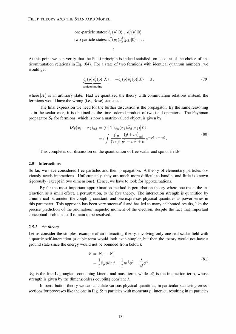
At this point we can verify that the Pauli principle is indeed satisfied, on account of the choice of an-ticommutation relations in Eq. (64). For a state of two fermions with identical quantum numbers, wewould get

b†i (p) b†i (p)︸︷︷︸

anticommuting

|X〉 = −b†i (p) b†i (p)|X〉 = 0 , (79)

where |X〉 is an arbitrary state. Had we quantized the theory with commutation relations instead, thefermions would have the wrong (i.e., Bose) statistics.

The final expression we need for the further discussion is the propagator. By the same reasoningas in the scalar case, it is obtained as the time-ordered product of two field operators. The Feynmanpropagator SF for fermions, which is now a matrix-valued object, is given by

iSF(x1 − x2)αβ =⟨0∣∣Tψα(x1)ψβ(x2)

∣∣ 0⟩

= i∫

d4p

(2π)4

(/p+m

)αβ

p2 −m2 + iεe−ip(x1−x2) .

(80)

This completes our discussion on the quantization of free scalar and spinor fields.

2.5 InteractionsSo far, we have considered free particles and their propagation. A theory of elementary particles ob-viously needs interactions. Unfortunately, they are much more difficult to handle, and little is knownrigorously (except in two dimensions). Hence, we have to look for approximations.

By far the most important approximation method is perturbation theory where one treats the in-teraction as a small effect, a perturbation, to the free theory. The interaction strength is quantified bya numerical parameter, the coupling constant, and one expresses physical quantities as power series inthis parameter. This approach has been very successful and has led to many celebrated results, like theprecise prediction of the anomalous magnetic moment of the electron, despite the fact that importantconceptual problems still remain to be resolved.

2.5.1 φ4 theoryLet us consider the simplest example of an interacting theory, involving only one real scalar field witha quartic self-interaction (a cubic term would look even simpler, but then the theory would not have aground state since the energy would not be bounded from below):

L = L0 + LI

=1

2∂µφ∂

µφ− 1

2m2φ2 − λ

4!φ4 .

(81)

L0 is the free Lagrangian, containing kinetic and mass term, while LI is the interaction term, whosestrength is given by the dimensionless coupling constant λ.

In perturbation theory we can calculate various physical quantities, in particular scattering cross-sections for processes like the one in Fig. 5: n particles with momenta pi interact, resulting inm particles

13


13

p1

...

pn

p′1

...

p′m

p1

...

pn

p2

p′1

pn

...

p′m

Fig. 5: Scattering of n incoming particles, pro-ducing m outgoing ones with momenta p1, . . . , pnand p′1, . . . , p

′m, respectively

Fig. 6: A disconnected diagram: One particledoes not participate in the interaction

with momenta p′j . Since the interaction is localized in a region of spacetime, particles are free at infinitepast and future. In other words, we have free asymptotic states

|p1, . . . , pn , in〉 at , t = −∞ and∣∣p′1, . . . , p′m , out

⟩at t = +∞ . (82)

The transition amplitude for the scattering process is determined by the scalar product of incoming andoutgoing states, which defines a unitary matrix, the so-called S-matrix (S for scattering),

⟨p′1, . . . , p

′m , out

∣∣ p1, . . . , pn , in⟩

=⟨p′1, . . . , p

′m

∣∣S∣∣ p1, . . . , pn

⟩. (83)

Detailed techniques have been developed to obtain a perturbative expansion for the S-matrix fromthe definition (83). The basis is Wick’s theorem and the LSZ formalism. One starts from a generalizationof the propagator, the time-ordered product of k fields,

τ(x1, . . . , xk) = 〈0 |Tφ(x1), . . . φ(xk)| 0〉 . (84)

First, disconnected pieces involving non-interacting particles have to be subtracted (see Fig. 6), and theblob in Fig. 5 decomposes into a smaller blob and straight lines just passing from the left to the rightside. From the Fourier transform

τ(x′1, . . . , x′m, x1, . . . , xn)

F.T.−→ τ(p′1, . . . , p′m, p1, . . . , pn) (85)

one then obtains the amplitude for the scattering process

⟨p′1, . . . , p

′m

∣∣S∣∣ p1, . . . , pn

⟩= (2π)4 δ4

(∑

out

p′i −∑

in

pi

)iM , (86)

where the matrix element M contains all the dynamics of the interaction. Because of the translationalinvariance of the theory, the total momentum is conserved. The matrix element can be calculated pertur-batively up to the desired order in the coupling λ via a set of Feynman rules. To calculate the cross-sectionfor a particular process, one first draws all possible Feynman diagrams with a given number of verticesand then translates them into an analytic expression using the Feynman rules.

For the φ4 theory, the Feynman diagrams are all composed out of three building blocks: Externallines corresponding to incoming or outgoing particles, propagators, and 4-vertices. The Feynman rulesread:

i. p 1 External lines: For each external line, multiply by 1 (i.e., exter-nal lines do not contribute to the matrix element in this theory).However, one needs to keep track of the momentum of each parti-cle entering or leaving the interaction. The momentum directionis indicated by the arrow.

14


14

ii. p ip2 −m2 + iε

Propagators between vertices are free propagators correspondingto the momentum of the particle. Note that particles of internallines need not be on-shell, i.e., p2 = m2 need not hold!

iii. −iλ Vertices yield a factor of the coupling constant. In this theory,there is only one species of particles, and the interaction termdoes not contain derivatives, so there is only one vertex, and itdoes not depend on the momenta.

iv. ∫d4p

(2π)4

The momenta of internal loops are not fixed by the incoming mo-menta. For each undetermined loop momentum p, one integratesover all values of p.

As an example, let us calculate the matrix element for the 2 → 2 scattering process to secondorder in λ. The relevant diagrams are collected in Fig. 7.

p1

p2

p3

p4

(a) Tree graph

p1

p2

p3

p4

p p+ p1 − p3

p1

p2

p3

p4

p

p1

p2

p3

p4

p

p1 + p2 − p

(b) One-loop graphs

Fig. 7: Feynman graphs for 2 → 2 scattering in φ4 theory to second order. The one-loop graphs are allinvariant under the interchange of the internal lines and hence get a symmetry factor of 1

2 .

The first-order diagram simply contributes a factor of −iλ, while the second-order diagrams involve anintegration:

iM = −iλ+1

2(−iλ)2

∫d4p

(2π)4

ip2 −m2

i(p+ p1 − p3)2 −m2

+1

2(−iλ)2

∫d4p

(2π)4

ip2 −m2

i(p+ p1 − p4)2 −m2

+1

2(−iλ)2

∫d4p

(2π)4

ip2 −m2

i(p1 + p2 − p)2 −m2

+O(λ3).

(87)

The factors of 12 are symmetry factors which arise if a diagram is invariant under interchange of internal

lines. The expression forM has a serious problem: The integrals do not converge. This can be seen bycounting the powers of the integration variable p. For p much larger than incoming momenta and themass, the integrand behaves like p−4. That means that the integral depends logarithmically on the upperintegration limit,

∫ Λ d4p

(2π)4

ip2 −m2

i(p+ p1 − p3)2 −m2

p pi,m−−−−−−−−−→∫ Λ d4p

(2π)4

−1

p4∝ ln Λ . (88)

15


15

Divergent loop diagrams are ubiquitous in quantum field theory. They can be cured by regularization,i.e., making the integrals finite by introducing some cutoff parameter, and renormalization, where thisadditional parameter is removed in the end, yielding finite results for observables. This will be discussedin more detail in the section on quantum corrections.

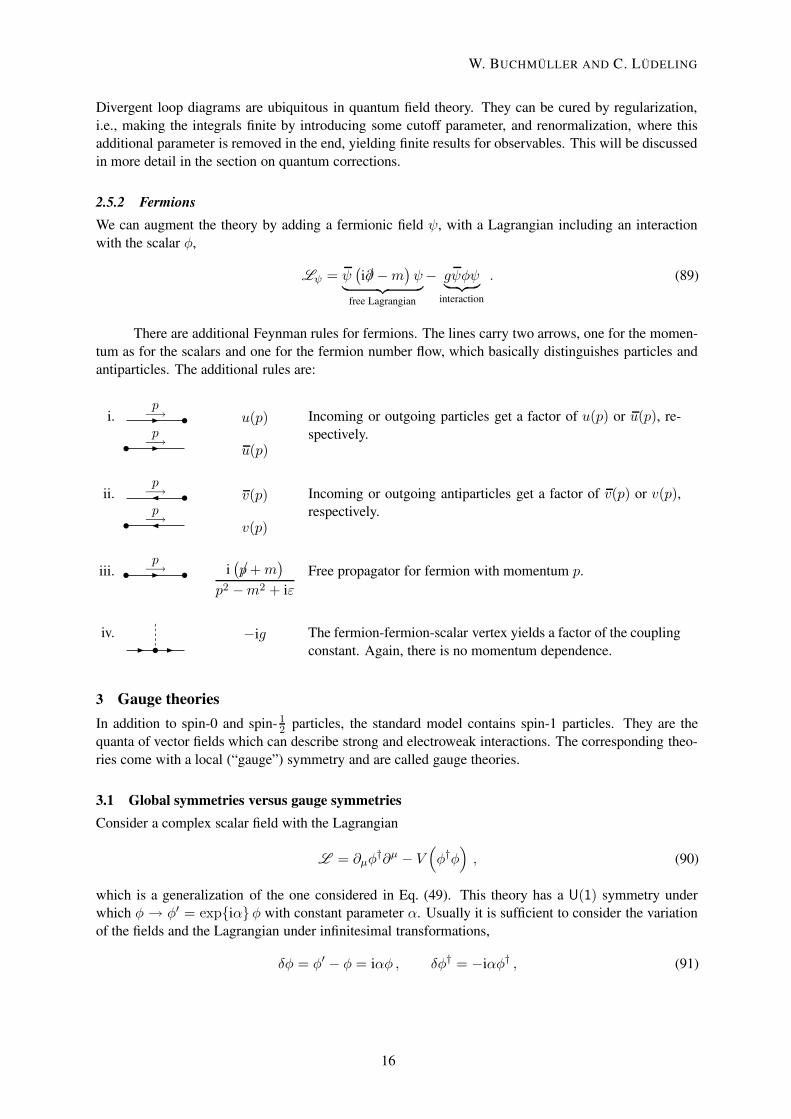
2.5.2 FermionsWe can augment the theory by adding a fermionic field ψ, with a Lagrangian including an interactionwith the scalar φ,

Lψ = ψ(i/∂ −m

)ψ︸︷︷︸

free Lagrangian

− gψφψ︸︷︷︸interaction

. (89)

There are additional Feynman rules for fermions. The lines carry two arrows, one for the momen-tum as for the scalars and one for the fermion number flow, which basically distinguishes particles andantiparticles. The additional rules are:

i.p−→p−→

u(p)

u(p)

Incoming or outgoing particles get a factor of u(p) or u(p), re-spectively.

ii.p−→p−→

v(p)

v(p)

Incoming or outgoing antiparticles get a factor of v(p) or v(p),respectively.

iii.p−→ i

(/p+m

)

p2 −m2 + iεFree propagator for fermion with momentum p.

iv. −ig The fermion-fermion-scalar vertex yields a factor of the couplingconstant. Again, there is no momentum dependence.

3 Gauge theoriesIn addition to spin-0 and spin- 1

2 particles, the standard model contains spin-1 particles. They are thequanta of vector fields which can describe strong and electroweak interactions. The corresponding theo-ries come with a local (“gauge”) symmetry and are called gauge theories.

3.1 Global symmetries versus gauge symmetriesConsider a complex scalar field with the Lagrangian

L = ∂µφ†∂µ − V

(φ†φ), (90)

which is a generalization of the one considered in Eq. (49). This theory has a U(1) symmetry underwhich φ → φ′ = expiαφ with constant parameter α. Usually it is sufficient to consider the variationof the fields and the Lagrangian under infinitesimal transformations,

δφ = φ′ − φ = iαφ , δφ† = −iαφ† , (91)

16


16

where terms O(α2)

have been neglected. To derive the Noether current, Eq. (51), we compute thevariation of the Lagrangian under such a transformation:

δL =∂L

∂φδφ+

∂L

∂φ†δφ† +

∂L

∂ (∂µφ)δ (∂µφ)︸︷︷︸=∂µδφ

+∂L

∂ (∂µφ†)δ(∂µφ

†)

=

(∂L

∂φ− ∂µ

∂L

∂ (∂µφ)

)

︸︷︷︸=0 by equation of motion

δφ+

(∂L

∂φ†− ∂µ

∂L

∂ (∂µφ†)

)

︸︷︷︸=0

δφ†

+ ∂µ

(∂L

∂ (∂µφ)δφ+

∂L

∂ (∂µφ†)δφ†)

= α∂µ

(i∂µφ†φ− iφ†∂µφ

)

= −α∂µjµ .

(92)

Since the Lagrangian is invariant, δL = 0, we obtain a conserved current for solutions of the equationsof motion,

∂µjµ = 0 . (93)

From the first to the second line we have used

∂L

∂ (∂µφ)∂µδφ = ∂µ

(∂L

∂ (∂µφ)δφ

)−(∂µ

∂L

∂ (∂µφ)

)δφ (94)

by the Leibniz rule.

The above procedure can be generalized to more complicated Lagrangians and symmetries. Thederivation does not depend on the precise form of L , and up to the second line of (92), it is independentof the form of δφ. As a general result, a symmetry of the Lagrangian always implies a conserved current,which in turn gives a conserved quantity (often referred to as charge, but it can be angular momentum orenergy as well).

What is the meaning of such a symmetry? Loosely speaking, it states that “physics does notchange” under such a transformation. This, however, does not mean that the solutions to the equations ofmotion derived from this Lagrangian are invariant under such a transformation. Indeed, generically theyare not, and only φ ≡ 0 is invariant.

As an example, consider the Mexican hat potential,

V (φ†φ) = −µ2φ†φ+ λ(φ†φ

)2. (95)

This potential has a ring of minima, namely all fields for which |φ|2 = µ2/(2λ). This means that anyconstant φ with this modulus is a solution to the equation of motion,

φ+∂V

∂φ

(φ, φ†

)= φ− φ†

(µ2 − 2λφ†φ

)= 0 . (96)

These solutions are not invariant under U(1) phase rotations. On the other hand, it is obvious that anysolution to the equations of motion will be mapped into another solution under such a transformation.

This situation is analogous to the Kepler problem: A planet moving around a stationary (verymassive) star. The setup is invariant under spatial rotations around the star, i.e., the symmetries formthe group SO(3). This group is three-dimensional (meaning that any rotation can be built from threeindependent rotations, e.g., around the three axes of a Cartesian coordinate system). Thus there are three

17


17

conserved charges which correspond to the three components of angular momentum. The solutions ofthis problem—the planet’s orbits—are ellipses in a plane, so they are not at all invariant under spatialrotations, not even under rotations in the plane of motion. Rotated solutions, however, are again solutions.

In particle physics, most experiments are scattering experiments at colliders. For those, the state-ment that “physics does not change” translates into “transformed initial states lead to transformed finalstates”: If one applies the transformation to the initial state and performs the experiment, the result willbe the same as if one had done the experiment with the untransformed state and transformed the result.

There is a subtle, but important, difference between this and another type of symmetry, gaugesymmetry. A gauge transformation is also a transformation which leaves the Lagrangian invariant, but itdoes relate identical states which describe exactly the same physics.

This might be familiar from electrodynamics. One formulation uses electric and magnetic fields~E and ~B, together with charge and current densities ρ and ~j. These fields and sources are related byMaxwell’s equations:

~∇× ~E +∂ ~B

∂t= 0 , ~∇ · ~B = 0 , (97a)

~∇× ~B − ∂ ~E

∂t= ~j , ~∇ · ~E = ρ . (97b)

The first two of these can be identically solved by introducing the potentials φ and ~A, which yield ~E and~B via

~E = −~∇φ− ∂ ~A

∂t, ~B = ~∇× ~A . (98)

So we have reduced the six components of ~E and ~B down to the four independent ones φ and ~A.However, the correspondence between the physical fields and the potentials is not unique. If somepotentials φ and ~A lead to certain ~E and ~B fields, the transformed potentials

~A′ = ~A+ ~∇Λ , φ′ = φ− ∂Λ

∂t, (99)

where Λ is a scalar field, give the same electric and magnetic fields.

This transformation (98) is called gauge transformation. It is a symmetry of the theory, but it isdifferent from the global symmetries we considered before. First, it is a local transformation, i.e., thetransformation parameter Λ varies in space and time. Second, it relates physically indistinguishable fieldconfigurations, since solutions of the equations of motion for electric and magnetic fields are invariant.It is important to note that this gauge transformation is inhomogeneous, i.e., the variation is not multi-plicative, but can generate non-vanishing potentials from zero. Potentials that are related to φ = 0 and~A = 0 by a gauge transformation are called pure gauge.

Phrased differently, we have expressed the physical fields ~E and ~B in terms of the potentials φand ~A. These potentials still contain too many degrees of freedom for the physical fields ~E and ~B,since different potentials can lead to the same ~E and ~B fields. So the description in terms of potentialsis redundant, and the gauge transformation (99) quantifies just this redundancy. Physical states andobservables have to be invariant under gauge transformations.

3.2 Abelian gauge theoriesThe easiest way to come up with a gauge symmetry is to start from a global symmetry and promoteit to a gauge one, that is, demand invariance of the Lagrangian under local transformations (where thetransformation parameter is a function of spacetime). To see this, recall the Lagrangian with the globalU(1) symmetry from the preceding section,

L = ∂µφ†∂µφ− V (φ†φ) ,

18


18

and the transformation

φ→ φ′ = eiαφ , δφ = φ′ − φ = iαφ .

If we now allow spacetime-dependent parameters α(x), the Lagrangian is no longer invariant. Thepotential part still is, but the kinetic term picks up derivatives of α(x), so the variation of the Lagrangianis

δL = i∂µα(∂µφ†φ− φ†∂µφ

)= −∂µα jµ , (100)

the derivative of α times the Noether current of the global symmetry derived before.

The way to restore invariance of the Lagrangian is to add another field, the gauge field, with agauge transformation just like the electromagnetic potentials in the previous section, combined into afour-vector Aµ = (φ, ~A):

Aµ(x)→ A′µ(x) = Aµ(x)− 1

e∂µα(x) . (101)

The factor 1e is included for later convenience. We can now combine the inhomogeneous transformation

of Aµ with the inhomogeneous transformation of the derivative in a covariant derivative Dµ:

Dµφ = (∂µ + ieAµ)φ . (102)

This is called covariant derivative because the differentiated object Dµφ transforms in the same way asthe original field,

Dµφ −→ (Dµφ)′ =(∂µ + ieA′µ

)φ′

= ∂µ

(eiα(x)φ

)+ ie

(Aµ(x)− 1

e∂µα(x)

)eiα(x)φ

= eiα(x)Dµφ .

(103)

So we can construct an invariant Lagrangian from the field and its covariant derivative:

L = (Dµφ)† (Dµφ)− V(φ†φ

). (104)

So far this is a theory of a complex scalar with U(1) gauge invariance. The gauge field Aµ,however, is not a dynamical field, i.e., there is no kinetic term for it. This kinetic term should be gaugeinvariant and contain derivatives up to second order. In order to find such a kinetic term, we first constructthe field strength tensor from the commutator of two covariant derivatives:

Fµν = − ie

[Dµ, Dν ] = − ie

[(∂µ + ieAµ) , (∂ν + ieAν)]

= − ie

([∂µ, ∂ν ] + [∂ν , ieAν ] + [ieAµ, ∂ν ]− e2 [Aµ, Aν ]

)

= ∂µAν − ∂νAµ .

(105)

To check that this is a sensible object to construct, we can redecompose Aµ into the scalar and vectorpotential φ and ~A and spell out the field strength tensor in electric and magnetic fields,

F µν =

0 −E1 −E2 −E3

E1 0 −B3 B2

E2 B3 0 −B1

E3 −B2 B2 0

. (106)

19


19

This shows that the field strength is gauge invariant, as are ~E and ~B. Of course, this can also be shownby straightforward calculation,

δFµν = ∂µδAν − ∂νδAµ = −1

e(∂µ∂ν − ∂ν∂µ)α(x) = 0 , (107)

so it is just the antisymmetry in µ and ν that ensures gauge invariance.

The desired kinetic term is now just the square of the field strength tensor,

Lgaugekin = −1

4FµνF

µν , (108a)

or, in terms of ~E and ~B fields,

L =1

2

(~E2 − ~B2

). (108b)

The coupling to scalar fields via the covariant derivative can also be applied to fermions. To couplea fermion ψ to the gauge field, one simply imposes the gauge transformation

ψ → ψ′ = eiαψ . (109)

In the Lagrangian, one again replaces the ordinary derivative with the covariant one. The Lagrangian fora fermion coupled to a U(1) gauge field is quantum electrodynamics (QED), if we call the fields electronand photon:

LQED = −1

4FµνF

µν + ψ(i /D −m

)ψ . (110)

Finally, let us note that for a U(1) gauge theory, different fields may have different charges underthe gauge group (as, for example, quarks and leptons indeed do). For fields with charge q (in unitsof elementary charge), we have to replace the gauge transformations and consequently the covariantderivative as follows:

ψq → ψ′q = eiqαψq , D(q)µ ψq = (∂µ + iqeAµ)ψq . (111)

What have we done so far? We started from a Lagrangian, Eq. (90) with a global U(1) symmetry(91). We imposed invariance under local transformations, so we had to introduce a new field, the gaugefield Aµ. This field transformed inhomogeneously under gauge transformations, just in a way to makea covariant derivative. This covariant derivative was the object that coupled the gauge field to the otherfields of the theory. To make this into a dynamical theory, we added a kinetic term for the gauge field,using the field strength tensor. Alternatively, we could have started with the gauge field and tried tocouple it to other fields, and we would have been led to the transformation properties (91). This is allwe need to construct the Lagrangian for QED. For QCD and the electroweak theory, however, we need aricher structure: non-Abelian gauge theories.

3.3 Non-Abelian gauge theoriesTo construct non-Abelian theories in the same way as before, we first have to discuss non-Abelian groups,i.e., groups whose elements do not commute. We shall focus on the groups SU(n), since they are mostrelevant for the Standard Model. SU(n) is the group of n×n complex unitary matrices with determinant1. To see how many degrees of freedom there are, we have to count: A n× n complex matrix U has n2

complex entries, equivalent to 2n2 real ones. The unitarity constraint, U †U =

, is a matrix equation,but not all component equations are independent. Actually, U †U is Hermitian,

(U †U

)†= U †U , so

20


20

the diagonal entries are real and the lower triangle is the complex conjugate of the upper one. Thus,there are n+ 2 · 1

2n(n− 1) real constraints. Finally, by taking the determinant of the unitarity constraint,det(U †U

)= |detU |2 = 1. Hence, restricting to detU = 1 eliminates one more real degree of freedom.

All in all, we have 2n2 − n − 2 · 12n(n − 1) − 1 = n2 − 1 real degrees of freedom in the elements of

SU(n).

This means that any U ∈ SU(n) can be specified by n2−1 real parameters αa. The group elementsare usually written in terms of these parameters and n2 − 1 matrices T a, the generators of the group, asan exponential

U = exp iαaT a =

+ iαaT a +O(α2), (112)

and one often considers only infinitesimal parameters.

The generators are usually chosen as Hermitian matrices3. The product of group elements trans-lates into commutation relations for the generators,

[T a, T b

]= ifabcT c , (113)

with the antisymmetric structure constants f abc, which of course also depend on the choice of generators.

In the Standard Model, the relevant groups are SU(2) for the electroweak theory and SU(3) forQCD. SU(2) has three parameters. The generators are usually chosen to be the Pauli matrices, T a = 1

2σa,

whose commutation relations are[σa, σb

]= iεabcσc. The common generators of SU(3) are the eight

Gell-Mann matrices, T a = 12λ

a.

To construct a model with a global SU(n) symmetry, we consider not a single field, but an n-component vector Φi, i = 1, . . . , n (called a multiplet of SU(n)), on which the matrices of SU(n) act bymultiplication:

Φ =

Φ1...

Φn

−→ Φ′ = UΦ , Φ† =

(Φ†1, · · · ,Φ†n

)−→

(Φ†)′

= Φ†U † . (114)

Now we see why we want unitary matrices U : A product Φ†Φ is invariant under such a transformation.This means that we can generalize the Lagrangian (90) in a straightforward way to include a non-Abeliansymmetry:

L = (∂µΦ)†(∂µΦ)− V(

Φ†Φ). (115)

If we allow for local transformations U = U(x), we immediately encounter the same problem asbefore: The derivative term is not invariant, because the derivatives act on the matrix U as well,

∂µΦ→ ∂µΦ′ = ∂µ (UΦ) = U∂µΦ + (∂µU) Φ . (116)

To save the day, we again need to introduce a covariant derivative consisting of a partial derivative plusa gauge field. This time, however, the vector field needs to be matrix-valued, i.e., Aµ = AaµT

a, whereT a are the generators of the group. We clearly need one vector field per generator, as each generatorrepresents an independent transformation in the group.

The transformation law of Aµ is chosen such that the covariant derivative is covariant,

(DµΦ)′ = [(∂µ + igAµ) Φ]′

=(∂µ + igA′µ

)(UΦ)

= U(∂µ + U−1 (∂µU) + igU−1A′µU

)Φ

!= UDµΦ .

(117)

3Actually, the generators live in the Lie algebra of the group, and so one can choose any basis one likes, Hermitian or not.

21


21

This requirement fixes the transformation of Aµ to be

A′µ = UAµU−1 − i

gU∂µU

−1 . (118)

In the Abelian case this reduces to the known transformation law, Eq. (101).

For infinitesimal parameters α = αaT a, the matrix U = expiα = 1 + iα, and Eq. (118)becomes

A′µ = Aµ −1

g∂µα+ i [α,Aµ] , (119)

or for each component

Aaµ′ = Aaµ −

1

g∂µα

a − fabcαbAcµ . (120)

Sometimes it is convenient to write down the covariant derivative in component form:

(DµΦ)i =(∂µδij + igT aijA

aµ

)Φj . (121)

Next we need a kinetic term, which again involves the field strength, the commutator of covariantderivatives:

Fµν = − ig

[Dµ, Dν ] = ∂µAν − ∂νAµ + ig [Aµ, aν ] = F aµνTa ,

F aµν = ∂µAaν − ∂νAaµ − gfabcAbµAcν .

(122)

Now we see that the field strength is more that just the derivative: There is a quadratic term in thepotentials. This leads to a self-interaction of gauge fields, like in QCD, where the gluons interact witheach other. This is the basic reason for confinement, unlike in QED, where the photon is not charged.

Furthermore, when we calculate the transformation of the field strength, we find that it is notinvariant, but transforms as

Fµν → F ′µν = UFµνU−1 , (123)

i.e., it is covariant. There is an easy way to produce an invariant quantity out of this: the trace. SincetrAB = trBA, the Lagrangian

L = −1

2tr (FµνF

µν) = −1

4F aµνF

a µν (124)

is indeed invariant, as tr(UF 2U−1

)= tr

(U−1UF 2

)= trF 2. In the second step we have used a

normalization convention,

tr(T aT b

)=

1

2δab , (125)

and every generator is necessarily traceless. The factor 12 is arbitrary and could be chosen differently,

with compensating changes in the coefficient of the kinetic term.

By choosing the gauge group SU(3) and coupling the gauge field to fermions, the quarks, we canwrite down the Lagrangian of quantum chromodynamics (QCD):

LQCD = −1

4GaµνG

a µν + q(i /D −m

)q , (126)

where a = 1, . . . , 8 counts the gluons and q is a three-component (i.e. three-colour) quark.

22


22

3.4 QuantizationSo far we have discussed only classical gauge theories. If we want to quantize the theory and find theFeynman rules for diagrams involving gauge fields, we have a problem: we have to make sure we do notcount field configurations of Aµ which are pure gauge, nor count separately fields which differ only bya gauge transformation, since those are meant to be physically identical. On the more technical side, thenaïve Green function for the free equation of motion does not exist. In the Abelian case, the equation is

∂µFµν = Aν − ∂ν∂µAµ = (gµν − ∂ν∂µ)Aµ = 0 . (127)

The Green function should be the inverse of the differential operator in brackets, but the operator is notinvertible. Indeed, it annihilates every pure gauge mode, as it should,

(gµν − ∂ν∂µ) ∂µΛ = 0 , (128)

so it has zero eigenvalues. Hence, the propagator must be defined in a more clever way.

One way out would be to fix the gauge, i.e., simply demand a certain gauge condition like ~∇· ~A = 0(Coulomb gauge) or nµAµ = 0 with a fixed 4-vector (axial gauge). It turns out, however, that the loss ofLorentz invariance causes many problems in calculations.

A better way makes use of Faddeev–Popov ghosts. In this approach, we add two terms to theLagrangian, the gauge-fixing term and the ghost term. The gauge-fixing term is not gauge invariant,but rather represents a certain gauge condition which can be chosen freely. The fact that it is not gaugeinvariant means that now the propagator is well defined, but the price to pay is that it propagates too manydegrees of freedom, namely gauge modes. This is compensated by the propagation of ghosts, strangefields which are scalars but which anticommute and do not show up as physical states but only as internallines in loop calculations. It turns out that gauge invariance is not lost but rather traded for a differentsymmetry, BRST symmetry, which ensures that we get physically sensible results.

For external states, we have to restrict to physical states, of which there are two for masslessbosons. They are labelled by two polarization vectors ε±µ which are transverse, i.e., orthogonal to themomentum four-vector and the spatial momentum, kµεµ = ~k~ε = 0.

The form of the gauge fixing and ghost terms depends on the gauge condition we want to take.A common (class of) gauge is the covariant gauge which depends on a parameter ξ, which becomesFeynman gauge (Landau/Lorenz gauge) for ξ = 1 (ξ = 0).

We now list the Feynman rules for a non-Abelian gauge theory (QCD) coupled to fermions(quarks) and ghosts. The fermionic external states and propagators are listed in Section 2.5.2.

i. k−→µk−→µ

εµ(k)

ε∗µ(k)

For each external line one has a polarization vector.

ii. pµ νa b

−iδab

k2 + iε

×(gµν + (1− ξ)kµkν

k2

)

The propagator for gauge bosons contains the pa-rameter ξ.

iii. ka b

−iδab

k2 + iεThe propagator for ghosts is the one of scalar parti-cles. There are no external ghost states.

iv. µ ieγµ In QED, there is just one vertex between photon andelectron.

23


23

v. µ i g2γµλa In QCD, the basic quark–quark–gluon vertex in-

volves the Gell-Mann matrices.

vi.

b c−→p

µ, a −gfabcpµ The ghosts couple to the gauge field.

vii. gfabckµ + permutations Three-gluon self-interaction.

viii. −14g

2fabcfadegµνgρσ

+permutations

Four-gluon self-interaction.

4 Quantum correctionsNow that we have the Feynman rules, we are ready to calculate quantum corrections [3, 5, 9]. As afirst example we consider the anomalous magnetic moment of the electron at one-loop order. This washistorically, and still is today, one of the most important tests of quantum field theory. The calculationis still quite simple because the one-loop expression is finite. In most cases, however, one encountersdivergent loop integrals. In the following sections we shall study these divergences and show how toremove them by renormalization. Finally, as an application, we shall discuss the running of couplingconstants and asymptotic freedom.

4.1 Anomalous magnetic momentThe magnetic moment of the electron determines its energy in a magnetic field,

Hmag = −~µ · ~B . (129)

For a particle with spin ~s, the magnetic moment is aligned in the direction of ~s, and for a classicalspinning particle of mass m and charge e, its magnitude would be the Bohr magneton, e/(2m). In thequantum theory, the magnetic moment is different, which is expressed by the Landé factor ge,

~µe = gee

2m~s . (130)

We now want to calculate ge in QED. To lowest order, this just means solving the Dirac equationin an external electromagnetic field Aµ = (φ, ~A),

(i /D −m

)ψ = [γµ (i∂µ − eAµ)−m]ψ = 0 . (131)

For a bound non-relativistic electron a stationary solution takes the form

ψ(x) =

(ϕ(~x)χ(~x)

)e−iEt , with

E −mm

1 . (132)

It is convenient to use the following representation of the Dirac matrices:

γ0 =

( 0

0 −

), γi =

(0 σi

−σi 0

). (133)

24


24

p p′

q µ

=

p p′

q µ

+

p p′k

q µ

+ · · ·

Fig. 8: Tree-level and one-loop diagram for the magnetic moment

One then obtains the two coupled equations

[(E − eφ)−m]ϕ−(−i~∇− e ~A

)· ~σχ = 0 , (134a)

[− (E − eφ)−m︸︷︷︸

≈−2m

]χ+

(−i~∇− e ~A

)· ~σϕ = 0 . (134b)

The coefficient of χ in the second equation is approximately independent of φ, so we can solve theequation to determine χ in terms of ϕ,

χ =1

m

(−i~∇− e ~A

)· ~σϕ . (135)

Inserting this into (134a), we get the Pauli equation,[

1

2m

(−i~∇− e ~A

)2+ eφ− e

2m~B · ~σ

]ϕ = (E −m)ϕ . (136)

This is a Schrödinger-like equation which implies (since ~s = 12~σ),

Hmag = −2e

2m~s~B . (137)

Hence, the Landé factor of the electron is ge = 2.

In QED, the magnetic moment is modified by quantum corrections. The magnetic moment is thespin-dependent coupling of the electron to a photon in the limit of vanishing photon momentum. Dia-grammatically, it is contained in the blob on the left side of Fig. 8, which denotes the complete electron–photon coupling. The tree-level diagram is the fundamental electron–photon coupling. There are severalone-loop corrections to this diagram, but only the so-called vertex correction, where an internal photonconnects the two electron lines, gives a contribution to the magnetic moment. All other one-loop dia-grams concern only external legs, such as an electron–positron bubble on the incoming photon, and willbe removed by wave-function renormalization.

The expression for the tree-level diagram is

iu(p′)eγµu(p) . (138)

Note that the photon becomes on-shell only for q → 0, so no polarization vector is included. The matrixelement of the electromagnetic current can be decomposed via the Gordon identity into convection andspin currents,

u(p′)γµu(p) = u(p′)(

(p+ p′)µ

2m+

i2m

σµν(p′ − p

)ν

)u(p) . (139)

25


25

Here the first term can be viewed as the net flow of charged particles, the second one is the spin current.Only this one is relevant for the magnetic moment, since it gives the spin-dependent coupling of theelectron.

In order to isolate the magnetic moment from the loop diagram, we first note that the correspondingexpression will contain the same external states, so it can be written as

iu(p′)eΓµ(p, q)u(p) , q = p′ − p , (140)

where Γµ(p, q) is the correction to the vertex due to the exchange of the photon. We can now decomposeΓµ into different parts according to index structure and extract the term∝σµν . Using the Feynman rules,we find for Γµ in Feynman gauge (ξ = 1),

ieΓµ(p, q) = (−ie)3∫

d4k

(2π)4

−igρσk2 + iε

γρi(/p′ − /k +m

)

(p′ − k)2 −m2 + iεγµ

× i(/p− /k +m

)

(p− k)2 −m2 + iεγσ .

(141)

This integral is logarithmically divergent, as can be seen by power counting, since the leading term is∝ k2 in the numerator and ∝ k6 in the denominator.

On the other hand, the part ∝σµνqµ is finite and can be extracted via some tricks:

– Consider first the denominator of the integral (141). It is the product of three terms of the form(momentum)2 −m2, which can be transformed into a sum at the expense of further integrationsover the so-called Feynman parameters x1 and x2,

1

A1A2A3= 2

∫ 1

0dx1

∫ 1−x1

0dx2

1

[A1x1 +A2x2 +A3 (1− x1 − x2)]3. (142)

– After introducing the Feynman parameters, the next trick is to shift the integration momentumk → k′, where

A1x1 +A2x2 +A3 (1− x1 − x2) =(k − x1p

′ − x2p)

︸︷︷︸k′

2 −(x1p′ + x2p

)2+ iε . (143)

Note that one must be careful when manipulating divergent integrals. In principle, one should firstregularize them and then perform the shifts on the regularized integrals, but in this case, there isno problem.

– For the numerator, the important part is the Dirac algebra of γ matrices. A standard calculationgives (see Appendix)

γν(/p ′ − /k +m

)γµ(/p− /k +m

)γν

= −2m2γµ − 4imσµν(p′ − p

)ν− 2/pγµ /p

′ +O(k) +O(k2).

(144)

Here we have used again the Gordon formula to trade (p+ p′)ν for σνρqρ, which is allowed onlyif the expression is sandwiched between on-shell spinors u(p′) and u(p).

– Now the numerator is split into pieces independent of k, linear and quadratic in k. The linear termcan be dropped under the integral. The quadratic piece leads to a divergent contribution which weshall discuss later. The integral over the k-independent part in the limit qµ → 0 yields

∫d4k

(2π)4

1[k2 − (x1 + x2)2 m2 + iε

]3 = − i32π2

1

(x1 + x2)2 m2. (145)

Now all that is left are the parameter integrals over x1 and x2.

26


26

Finally, one obtains the result, usually expressed in terms of the fine structure constant α =e2/ (4π),

ieu(p′)Γµu(p) = +ieu(p′)(α

2π

i2m

σµνqν + · · ·)u(p) , (146)

where the dots represent contributions which are not ∝ σµνqν .

Comparison with the Gordon decomposition (139) gives the one-loop correction to the Landéfactor,

g = 2(

1 +α

2π

). (147)

This correction was first calculated by Schwinger in 1948. It is often expressed as the anomalous mag-netic moment ae,

ae =g − 2

2. (148)

Today, ae is known up to three loops analytically and to four loops numerically [10]. The agreement oftheory and experiment is impressive:

aexpe = (1159652185.9 ± 3.8) · 10−12 ,

athe = (1159652175.9 ± 8.5) · 10−12 .

(149)

This is one of the cornerstones of our confidence in quantum field theory.

4.2 DivergencesThe anomalous magnetic moment we calculated in the last section was tedious work, but at least the resultwas finite. Most other expressions, however, have divergent momentum integrals. One such example isthe vertex function Γµ we already considered. It has contributions which are logarithmically divergent.We can isolate these by setting q = 0, which yields

Γµ(p, 0) = −2ie2

∫ 1

0dx1

∫ 1−x1

0dx2

∫d4k

(2π)2

γν /kγµ /kγν[k2 − (x1 + x2)2m2 + iε

]3 . (150)

This expression is treated in two steps:

– First we make the integral finite in a step called regularization. In this step, we have to introducea new parameter of mass dimension 1. An obvious choice would be a cutoff Λ which servesas an upper bound for the momentum integration. One might even argue that there should be acutoff at a scale where quantum gravity becomes important, although a regularization parameterhas generally no direct physical meaning.

– The second step is renormalization. The divergences are absorbed into the parameters of the theory.The key idea is that the ‘bare’ parameters which appear in the Lagrangian are not physical, so theycan be divergent. Their divergences are chosen such as to cancel the divergences coming from thedivergent integrals.

– Finally, the regulator is removed. Since all divergences have been absorbed into the parametersof the theory, the results remain finite for infinite regulator. Of course, one has to make sure theresults do not depend on the regularization method.

The cutoff regularization, while conceptually simple, is not a convenient method, as it breaksLorentz and gauge invariance. Symmetries, however, are very important for all calculations, so a goodregularization scheme should preserve as many symmetries as possible. We shall restrict ourselves todimensional regularization, which is the most common scheme used nowadays.

27


27

4.2.1 Dimensional regularizationThe key idea is to define the theory not in four, but in d = 4 − ε dimensions [9]. If ε is not an integer,the integrals do converge. Non-integer dimensionality might seem weird, but in the end we shall take thelimit of ε → 0 and return to four dimensions. This procedure is well defined and just an intermediatestep in the calculation.

Let us consider some technical issues. In d dimensions, the Lorentz indices ‘range from 0 to d’,in the sense that

gµνgνµ = d , (151)

and there are d γ-matrices obeying the usual algebra,

γµ, γν = 2gµν, tr (

) = 4 . (152)

The γ-matrix contractions are also modified due to the change in the trace of gµν , such as

γµγνγµ = − (2− ε) γν , γµγνγργµ = 4gνρ − εγνγρ . (153)

The tensor structure of diagrams can be simplified as follows. If a momentum integral over k containsa factor of kµkν , this must be proportional to gµνk2, since it is of second order in k and symmetric in(µν). The only symmetric tensor we have is the metric (as long as the remaining integrand depends onlyon the square of k and the squares of the external momenta pi), and the coefficient can be obtained bycontracting with gµν to yield

∫d4k

(2π)4kµkνf(k2, p2

i

)=

1

dgµν

∫d4k

(2π)4 k2f(k2, p2

i

). (154)

The measure of an integral changes from d4k to ddk. Since k is a dimensionful quantity4 (ofmass dimension 1), we need to compensate the change in dimensionality by a factor of µε, where µ isan arbitrary parameter of mass dimension 1. The mass dimensions of fields and parameters also change.They can be derived from the condition that the action, which is the d-dimensional integral over theLagrangian, be dimensionless. Schematically (i.e., without all numerical factors), a Lagrangian of gaugefields, scalars and fermions reads

L = (∂µAν)2 + e∂µAµAνA

ν + e2 (AµAµ)2

+ (∂µφ)2 + ψ(i/∂ −m

)ψ + eψ /Aψ +m2φ2 + · · · .

(155)

The condition of dimensionless action, [S] = 0, translates into [L ] = d, since[ddx]

= −d. Derivativeshave mass dimension 1, and so do masses. That implies for the dimensions of the fields (and the limit asd→ 4),

[Aµ] =d− 2

2→ 1 , [φ] =

d− 2

2→ 1 , (156)

[ψ] =d− 1

2→ 3

2, [e] = 2− d

2→ 0 . (157)

How do we evaluate a d-dimensional integral? One first transforms to Euclidean space replacingk0 by ik4, so that the Lorentzian measure ddk becomes ddkE. In Euclidean space, one can easily convert

4In our units where ~ = c = 1, the only dimension is mass, so everything can be expressed in powers of GeV. The basicquantities have [mass] = [energy] = [momentum] = 1 and [length] = [time] = −1, so [dxµ] = −1 and [∂µ] = 1.

28


28

pp− k

k

p = −iΣ (p)

(a) The electron self-energy

µ νqq

p+ q

p

= −iΠµν (q)

(b) The vacuum polarization

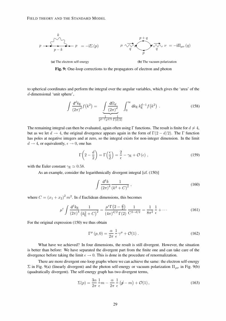
Fig. 9: One-loop corrections to the propagators of electron and photon

to spherical coordinates and perform the integral over the angular variables, which gives the ‘area’ of thed-dimensional ‘unit sphere’,

∫ddkE

(2π)df(k2)

=

∫dΩd

(2π)d︸︷︷︸1

2d−1πd/21

Γ(d/2)

∫ ∞

0dkE k

d−1E f

(k2). (158)

The remaining integral can then be evaluated, again often using Γ functions. The result is finite for d 6= 4,but as we let d → 4, the original divergence appears again in the form of Γ(2− d/2). The Γ functionhas poles at negative integers and at zero, so the integral exists for non-integer dimension. In the limitd→ 4, or equivalently, ε→ 0, one has

Γ

(2− d

2

)= Γ

( ε2

)=

2

ε− γE +O (ε) , (159)

with the Euler constant γE ' 0.58.

As an example, consider the logarithmically divergent integral [cf. (150)]∫

d4k

(2π)4

1

(k2 + C)2 , (160)

where C = (x1 + x2)2 m2. In d Euclidean dimensions, this becomes

µε∫

d4kE

(2π)4

1(k2

E +C)2 =

µεΓ(2− d

2

)

(4π)d/2 Γ(2)

1

C2−d/2 =1

8π2

1

ε+ · · · (161)

For the original expression (150) we thus obtain

Γµ (p, 0) =α

2π

1

εγµ +O(1) . (162)

What have we achieved? In four dimensions, the result is still divergent. However, the situationis better than before: We have separated the divergent part from the finite one and can take care of thedivergence before taking the limit ε→ 0. This is done in the procedure of renormalization.

There are more divergent one-loop graphs where we can achieve the same: the electron self-energyΣ in Fig. 9(a) (linearly divergent) and the photon self-energy or vacuum polarization Πµν in Fig. 9(b)(quadratically divergent). The self-energy graph has two divergent terms,

Σ(p) =3α

2π

1

εm− α

2π

1

ε

(/p−m

)+O(1) , (163)

29


29

which contribute to the mass renormalization and the wave function renormalization, respectively. Thevacuum polarization seems more complicated since it is a second rank tensor. However, the tensorstructure is fixed by gauge invariance which requires

qµΠµν (q) = 0 . (164)

Therefore, because of Lorentz invariance,

Πµν (q) =(gµνq

2 − qµqν)

Π(q2). (165)

The remaining scalar quantity Π(q2) has the divergent part

Π(q2)

=2α

3π

1

ε+O(1) . (166)

4.2.2 RenormalizationSo far we have isolated the divergences, but they are still there. How do we get rid of them? The crucialinsight is that the parameters of the Lagrangean, the ‘bare’ parameters, are not observable. Rather,the sum of bare parameters and loop-induced corrections are physical. Hence, divergencies of bareparameters can cancel against divergent loop corrections, leaving physical observables finite.

To make this more explicit, let us express, as an example, the QED Lagrangian in terms of barefields Aµ0 and ψ0 and bare parameters m0 and e0,

L = −1

4(∂µA0 ν − ∂νA0 µ)

(∂µA0 ν − ∂νA0 µ

)+ ψ0 (γµ (i∂µ − e0A0µ)−m0)ψ0 . (167)

The ‘renormalized fields’ Aµ and ψ and the ‘renormalized parameters’ e and m are then obtained fromthe bare ones by multiplicative rescaling,

A0µ =√Z3Aµ , ψ0 =

√Z2ψ , (168)

m0 =ZmZ2

m , e0 =Z1

Z2

√Z3µ2−d/2e . (169)

Note that coupling and electron mass now depend on the mass parameter µ,

e = e(µ) , m = m(µ) . (170)

In terms of the renormalized fields and parameters the Lagrangian (167) reads

L = −1

4(∂µAν − ∂νAµ) (∂µAν − ∂νAµ) + ψ (γµ (i∂µ − eAµ)−m)ψ + ∆L , (171)

where ∆L contains the divergent counterterms,

∆L = − (Z3 − 1)1

4FµνF

µν + (Z2 − 1)ψi/∂ψ

− (Zm − 1)mψψ − (Z1 − 1) eψ /Aψ .(172)

The counter-terms have the same structure as the original Lagrangian and lead to new vertices in theFeynman rules:

i.µ

q

ν−i (Z3 − 1)×(gµνq

2 − qµqν) Photon wave function counter-term (counter-terms are

generically denoted by ). It has the same tensor struc-ture as the vacuum polarization.

30


30

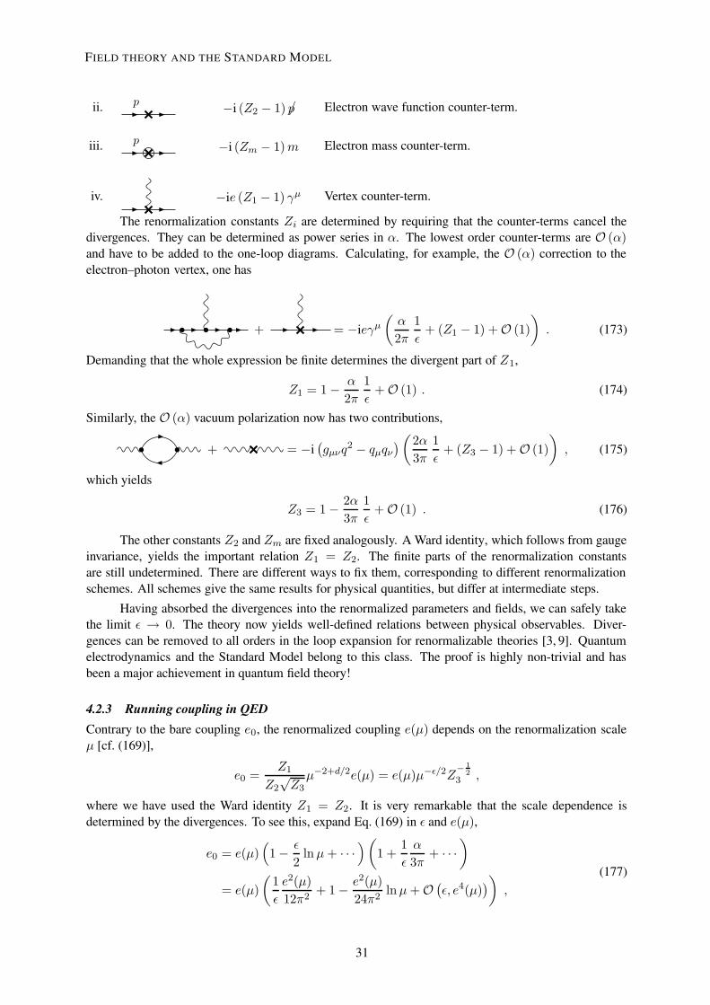
ii. p −i (Z2 − 1) /p Electron wave function counter-term.

iii. p −i (Zm − 1)m Electron mass counter-term.

iv. −ie (Z1 − 1) γµ Vertex counter-term.

The renormalization constants Zi are determined by requiring that the counter-terms cancel thedivergences. They can be determined as power series in α. The lowest order counter-terms are O (α)and have to be added to the one-loop diagrams. Calculating, for example, the O (α) correction to theelectron–photon vertex, one has

+ = −ieγµ(α

2π

1

ε+ (Z1 − 1) +O (1)

). (173)

Demanding that the whole expression be finite determines the divergent part of Z1,

Z1 = 1− α

2π

1

ε+O (1) . (174)

Similarly, the O (α) vacuum polarization now has two contributions,

+ = −i(gµνq

2 − qµqν)(2α

3π

1

ε+ (Z3 − 1) +O (1)

), (175)

which yields

Z3 = 1− 2α

3π

1

ε+O (1) . (176)

The other constants Z2 and Zm are fixed analogously. A Ward identity, which follows from gaugeinvariance, yields the important relation Z1 = Z2. The finite parts of the renormalization constantsare still undetermined. There are different ways to fix them, corresponding to different renormalizationschemes. All schemes give the same results for physical quantities, but differ at intermediate steps.

Having absorbed the divergences into the renormalized parameters and fields, we can safely takethe limit ε → 0. The theory now yields well-defined relations between physical observables. Diver-gences can be removed to all orders in the loop expansion for renormalizable theories [3, 9]. Quantumelectrodynamics and the Standard Model belong to this class. The proof is highly non-trivial and hasbeen a major achievement in quantum field theory!

4.2.3 Running coupling in QEDContrary to the bare coupling e0, the renormalized coupling e(µ) depends on the renormalization scaleµ [cf. (169)],

e0 =Z1

Z2

√Z3µ−2+d/2e(µ) = e(µ)µ−ε/2Z

− 12

3 ,

where we have used the Ward identity Z1 = Z2. It is very remarkable that the scale dependence isdetermined by the divergences. To see this, expand Eq. (169) in ε and e(µ),

e0 = e(µ)(

1− ε

2lnµ+ · · ·

)(1 +

1

ε

α

3π+ · · ·

)

= e(µ)

(1

ε

e2(µ)

12π2+ 1− e2(µ)

24π2lnµ+O

(ε, e4(µ)

)),

(177)

31


31

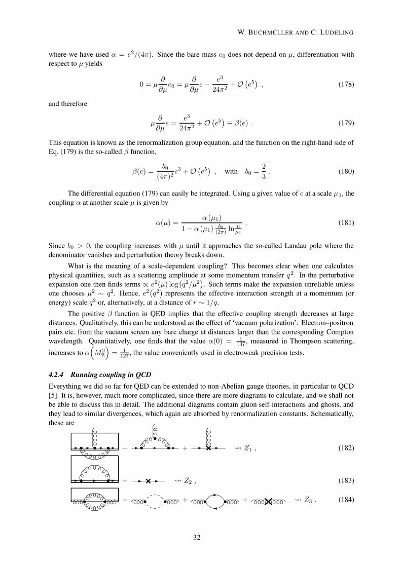
where we have used α = e2/(4π). Since the bare mass e0 does not depend on µ, differentiation withrespect to µ yields

0 = µ∂

∂µe0 = µ

∂

∂µe− e3

24π2+O

(e5), (178)

and therefore

µ∂

∂µe =

e3

24π2+O

(e5)≡ β(e) . (179)

This equation is known as the renormalization group equation, and the function on the right-hand side ofEq. (179) is the so-called β function,

β(e) =b0

(4π)2e3 +O

(e5), with b0 =

2

3. (180)

The differential equation (179) can easily be integrated. Using a given value of e at a scale µ1, thecoupling α at another scale µ is given by

α(µ) =α (µ1)

1− α (µ1) b0(2π) ln µ

µ1

. (181)

Since b0 > 0, the coupling increases with µ until it approaches the so-called Landau pole where thedenominator vanishes and perturbation theory breaks down.

What is the meaning of a scale-dependent coupling? This becomes clear when one calculatesphysical quantities, such as a scattering amplitude at some momentum transfer q2. In the perturbativeexpansion one then finds terms ∝ e2(µ) log

(q2/µ2

). Such terms make the expansion unreliable unless

one chooses µ2 ∼ q2. Hence, e2(q2)

represents the effective interaction strength at a momentum (orenergy) scale q2 or, alternatively, at a distance of r ∼ 1/q.

The positive β function in QED implies that the effective coupling strength decreases at largedistances. Qualitatively, this can be understood as the effect of ‘vacuum polarization’: Electron–positronpairs etc. from the vacuum screen any bare charge at distances larger than the corresponding Comptonwavelength. Quantitatively, one finds that the value α(0) = 1

137 , measured in Thompson scattering,

increases to α(M2

Z

)= 1

127 , the value conveniently used in electroweak precision tests.

4.2.4 Running coupling in QCDEverything we did so far for QED can be extended to non-Abelian gauge theories, in particular to QCD[5]. It is, however, much more complicated, since there are more diagrams to calculate, and we shall notbe able to discuss this in detail. The additional diagrams contain gluon self-interactions and ghosts, andthey lead to similar divergences, which again are absorbed by renormalization constants. Schematically,these are

+ + Z1 , (182)

+ Z2 , (183)

+ + + Z3 . (184)

32


32

The renormalized coupling can again be defined as in QED, Eq. (169),

g0 =Z1

Z2

√Z3µ−2+d/2 g . (185)

The coefficients of the 1/ε-divergences depend on the gauge group and on the number of differentfermions. For a SU(Nc) gauge group with Nf flavours of fermions, one obtains the β function forthe gauge coupling g,

µ∂

∂µg =

b0

(4π)2 g3 +O

(g5), b0 = −

(11

3Nc −

4

3Nf

). (186)

Note that forNf < 11Nc/4 the coefficient is negative! Hence, the coupling decreases at high-momentumtransfers or short distances. The calculation of this coefficient earned the Nobel Prize in 2004 for Gross,Politzer and Wilczek. The decrease of the coupling at short distances is the famous phenomenon ofasymptotic freedom. As a consequence, one can treat in deep-inelastic scattering quarks inside theproton as quasi-free particles, which is the basis of the parton model.

The coupling at a scale µ can again be expressed in terms of the coupling at a reference scale µ1,

α(µ) =α (µ1)

1 + α (µ1) |b0|(2π) ln µµ1

. (187)

The analogue of the Landau pole now occurs at small µ or large distances. For QCD withNc = 3 andNf = 6, the pole is at the ‘QCD scale’ ΛQCD ' 300 MeV. At the QCD scale gluons and quarks arestrongly coupled and colour is confined [5]. Correspondingly, the inverse of ΛQCD gives roughly the sizeof hadrons, rhad ∼ Λ−1

QCD ∼ 0.7 fm.

5 Electroweak theorySo far we have studied QED, the simplest gauge theory, and QCD, the prime example of a non-Abeliangauge theory. But there also are the weak interactions, which seem rather different. They are short-ranged, which requires massive messenger particles, seemingly inconsistent with gauge invariance. Fur-thermore, weak interactions come in two types, charged and neutral current–current interactions, whichcouple quarks and leptons differently. Charged-current interactions, mediated by the W ± bosons, onlyinvolve left-handed fermions and readily change flavour, as in the strange quark decay s → ue−νe.Neutral-current interactions, on the other hand, couple both left- and right-handed fermions, and flavour-changing neutral currents are strongly suppressed.

Despite these differences from QED and QCD, weak interactions also turn out to be described bya non-Abelian gauge theory. Yet the electroweak theory is different for two reasons: it is a chiral gaugetheory, and the gauge symmetry is spontaneously broken.

5.1 Quantum numbersIn a chiral gauge theory, the building blocks are massless left- and right-handed fermions,

ψL =1

2

(1− γ5

)ψL , ψR =

1

2

(1 + γ5

)ψR , (188)

with different gauge quantum numbers. For one generation of Standard Model particles, we have sevenchiral spinors: Two each for up- and down-type quark and charged lepton, and just one for the neutrinowhich we shall treat as massless in this section, i.e., we omit the right-handed one. The electroweakgauge group is a product of two groups, GEW = SU(2)W × U(1)Y . Here the subscript W stands for‘weak isospin’, which is the quantum number associated with the SU(2)W factor, and the U(1) charge isthe hypercharge Y .

33


33

The assignment of quantum numbers, which corresponds to the grouping into representationsof the gauge group, is obtained as follows: The non-Abelian group SU(2)W has a chargeless one-dimensional singlet (1) representation and charged multidimensional representations, starting with thetwo-dimensional doublet (2) representation5 . We are not allowed to mix quarks and leptons, since weakinteractions do not change colour, nor left- and right-handed fields, which would violate Lorentz sym-metry. The U(1)Y factor is Abelian, so it has only one-dimensional representations. This means we canassign different hypercharges to the various singlets and doublets of SU(2)W .

Furthermore, we know that charged currents connect up- with down-type quarks and chargedleptons with neutrinos, and that the W± bosons couple only to left-handed fermions. This suggests toform doublets from uL and dL, and from eL and νL, and to keep the right-handed fields as singlets. Sowe obtain the SU(2)W multiplets

qL =

(uLdL

), uR , dR , lL =

(νLeL

), eR , (189)

with the hypercharges (which we shall justify later)

field: qL uR dR lL eR

hypercharge: 16

23 −1

3 −12 −1

. (190)

With these representations, we can write down the covariant derivatives. The SU(2)W has threegenerators, which we choose to be the Pauli matrices, and therefore three gauge fields W I

µ , I = 1, 2, 3.The U(1)Y gauge field is Bµ, and the coupling constants are g and g ′, respectively. The covariantderivatives acting on the left-handed fields are

DµψL =(∂µ + igWµ + ig′Y Bµ

)ψL , where Wµ = 1

2σIW I

µ , (191)

while the right-handed fields are singlets under SU(2)W , and hence do not couple to the W bosons,

DµψR =(∂µ + ig′Y Bµ

)ψR . (192)

From the explicit form of the Pauli matrices,

σ1 =

(0 11 0

), σ2 =

(0 −ii 0

), σ3 =

(1 00 −1

), (193)

we see that W 1µ and W 2

µ mix up- and down-type quarks, while W 3µ does not, like the U(1) boson Bµ.

It is often convenient to split the Lagrangian into the free (kinetic) part and the interaction La-grangian, which takes the form (current) · (vector field). In the electroweak theory, one has

Lint = −gJ IW, µW I µ − g′JY, µBµ , (194)

with the currents

JIW,µ = qLγµ12σ

IqL + lLγµ12σ

I lL , (195)

JY, µ =1

6qLγµqL −

1

2lLγµlL +

2

3uRγµuR −

1

3dRγµdR − eRγµeR . (196)

These currents have to be conserved, ∂µJµ = 0, to allow a consistent coupling to gauge bosons.

5Here we use ‘representation’ as meaning ‘irreducible representation’. Of course we can build reducible representations ofany dimension.

34


34

5.1.1 AnomaliesBefore considering the Higgs mechanism which will lead to the identification of the physical W±, Zand γ bosons of the Standard Model, let us briefly discuss anomalies. We shall see that the choice ofhypercharges in (190) is severely constrained by the consistency of the theory.

Suppose we have a classical field theory with a certain symmetry and associated conserved cur-rent. After quantizing the theory, the resulting quantum field theory might not have that symmetry anymore, which means the current is no longer conserved. This is called an anomaly. Anomalies are nota problem for global symmetries, where the quantized theory just lacks that particular symmetry. Forgauge symmetries, however, the currents have to be conserved, otherwise the theory is inconsistent.

A ∝ JA

JB

JC

ψL

− JA

JB

JC

ψR

Fig. 10: The gauge anomaly is given by triangle diagrams with chiral fermions in the loop

Anomalies are caused by certain one-loop diagrams, the so-called triangle diagrams (see Fig. 10).The left- and right-handed fermions contribute with different sign, so if they have the same quantumnumbers, the anomaly vanishes. This is the case in QED and QCD, which thus are automatically anomalyfree. In general, for currents JA, JB and JC , the anomaly A is the difference of the traces of thegenerators TA, TB and TC in the left- and right-handed sectors,

A = tr[TA, TB

TC]L− tr

[TA, TB

TC]R

!= 0 . (197)

Here the trace is taken over all fermions. For the electroweak theory, in principle there are four com-binations of currents, containing three, two, one or no SU(2)W current. However, the trace of any oddnumber of σI matrices vanishes, so we only have to check the SU(2)2

WU(1)Y and U(1)3Y anomalies.

The SU(2)W generators are 12σ

I , whose anticommutator is

12σ

I , 12σ

J

= 12δIJ . Furthermore,

only the left-handed fields contribute, since the right-handed ones are SU(2)W singlets. Hence theSU(2)2

WU(1)Y anomaly is

A = tr

[1

2σI ,

1

2σJY

]

L

=1

2δIJ tr [Y ]L =

1

2δIJ

(3︸︷︷︸Nc

·16− 1

2

)= 0 . (198)

We see that it vanishes only if quarks come in three colours!

The U(1)3Y anomaly also vanishes:

A = tr [Y, Y Y ]L − tr [Y, Y Y ]R = 2(

tr[Y 3]L− tr

[Y 3]R

)

= 2

(3 · 2

(1

6

)3

+ 2

(−1

2

)3

− 3

(2

3

)3

− 3

(−1

3

)3

− (−1)3

)

= 0 .

(199)

This vanishing of the anomaly is again related to the number of colours. It does not vanish in eitherthe left- or right-handed sector, nor in the quark and lepton sector individually. Hence the vanishing of

35


35

anomalies provides a deep connection between quarks and leptons in the Standard Model, which is a hintto grand unified theories where anomaly cancellation is often automatic.

Anomaly cancellation is not restricted to the electroweak gauge currents, but applies to the strongforce and gravity as well: Mixed SU(3)C -U(1)Y anomalies vanish by the same argument as above:Only the SU(3)2

CU(1)Y triangle contributes, but it is tr [Y ]L − tr [Y ]R = 0. The same is true for thelast possible anomaly, the gravitational one, where two non-Abelian gauge currents are replaced by theenergy-momentum tensor Tµν .

Hence, the Standard Model is anomaly free, as it should be. For this, all particles of one generationwith their strange hypercharges have to conspire to cancel the different anomalies. A ‘Standard Model’without quarks, for instance, would not be a consistent theory, nor would a ‘Standard Model’ with fourcolours of quarks. Note that a right-handed neutrino, suggested by neutrino masses, does not pose anyproblem, since it is a complete singlet, without any charge, and thus it does not contribute to any gaugeanomaly.

5.2 Higgs mechanismThe electroweak model discussed so far bears little resemblance to the physics of weak interactions. Thegauge bosons W I

µ and Bµ are massless, implying long-range forces, because a mass term m2WµWµ

would violate gauge invariance. Furthermore, the fermions are massless as well, again because of gaugeinvariance: a mass term mixes left- and right-handed fermions,

mψψ = m(ψLψR + ψRψL

), (200)

and since these have different gauge quantum numbers, such a term is not gauge invariant. The wayout is the celebrated Higgs mechanism: Spontaneous symmetry breaking generates masses for the gaugebosons and fermions without destroying gauge invariance. A simpler version of this effect is what hap-pens in superconductors: the condensate of Cooper pairs induces an effective mass for the photon, sothat electromagnetic interactions become short-ranged, leading to the Meissner–Ochsenfeld effect whereexternal magnetic fields are expelled from the superconductor, levitating it.

The key ingredient for the Higgs mechanism is a complex scalar field Φ, which is a doublet underSU(2)W with hypercharge − 1

2 , which has four real degrees of freedom. The crucial feature of the Higgsfield is its potential, which is of the Mexican hat form:

L = (DµΦ)† (DµΦ)− V(

Φ†Φ), (201)

with

DµΦ =

(∂µ + igWµ −

i2g′Bµ

)Φ ,

V(

Φ†Φ)

= −µ2 Φ†Φ +1

2λ(

Φ†Φ)2

, µ2 > 0 . (202)

This potential has a minimum away from the origin, at Φ†Φ = v2 ≡ µ2/λ. In the vacuum, the Higgsfield settles in this minimum. At first sight, the minimization of the potential only fixes the modulusΦ†Φ, i.e., one of the four degrees of freedom. The other three, however, can be eliminated by a gaugetransformation, and we can choose the following form of Φ, which is often referred to as unitary gauge:

Φ =

(0

v + 1√2H(x)

), H = H∗ . (203)

Here we have eliminated the upper component and the imaginary part of the lower one. We have alsoshifted the lower component to the vacuum value, so that the dynamical field H(x) vanishes in thevacuum.

36


36

In unitary gauge, the Higgs Lagrangian (201) becomes

L =λ

2v4

+1

2∂µH ∂µH − λv2H2 +

λ√2vH3 +

λ

8H4

+1

4

(v +

1√2H

)2 (W 1µ ,W

2µ ,W

3µ , Bµ

)

g2 00 g2 0

0 g2 gg′

gg′ g′2

W 1µ

W 2µ

W 3µ

Bµ

.

(204)

The first line could be interpreted as vacuum energy density, i.e., a cosmological constant. However,such an interpretation is on shaky grounds in quantum field theory, so we shall ignore this term6. Thesecond line describes a real scalar field H of mass m2

H = 2λv2 with cubic and quartic self-interactions.The most important line, however, is the last one: It contains mass terms for the vector bosons! A closerlook at the mass matrix reveals that it only is of rank three, so it has one zero eigenvalue, and the threeremaining ones are g2, g2, and

(g2 + g′2

). In other words, it describes one massless particle, two of

equal non-zero mass, and one which is even heavier, i.e., we have identified the physical γ, W± and Zbosons.

The massless eigenstate of the mass matrix, i.e., the photon, is the linear com-bination Aµ = − sin θWW

3µ + cos θWBµ, the orthogonal combination is the Z boson,

Zµ = cos θWW3µ + sin θWBµ. Here we have introduced the Weinberg angle θW, which is defined

by

sin θW =g′√

g2 + g′2, cos θW =

g√g2 + g′2

. (205)

To summarize, the theory contains the following mass eigenstates:

– Two charged vector bosons W± with mass M 2W = 1

2g2v2,

– two neutral vector bosons with masses MZ = 12

(g2 + g′2

)v2 = M2

W cos−2 θW and Mγ = 0,– and one neutral Higgs boson with mass m2

H = 2λv2.

The Higgs mechanism and the diagonalization of the vector boson mass matrix allow us to rewritethe interaction Lagrangian (194), which was given in terms of the old fields W I

µ and Bµ and their cur-rents (195) and (196), in terms of the physical field. The associated currents are separated into a chargedcurrent (for W±µ ) and neutral currents (for Aµ and Zµ):

LCC = − g√2

∑

i=1,2,3

(uLiγµdLi + νLiγ

µeLi)W+µ + h.c. , (206)

LNC = −gJ3µW

3µ − g′JY µBµ

= −eJem µAm − e

sin 2θWJZ µZ

µ ,(207)

with the electromagnetic and Z currents

Jemµ =∑

i=u,d,c,s,t,b,e,µ,τ

ψiγµQiψi , with the electric charge Qi = T 3i + Yi , (208)

6Generally, nothing prevents us from adding an arbitrary constant to the Lagrangian, obtaining any desired ‘vacuum energy’.For example, the Higgs potential is often written as

`Φ†Φ − v2

´2, so that its expectation value vanishes in the vacuum. These

potentials just differ by the shift ∼ v4, and are indistinguishable within QFT.

37


37

JZ µ =∑

i=u,d,c,s,t,be,µ,τ,νe,νµ,ντ

ψiγµ(vi − aiγ5

)ψi . (209)

Here the fermions ψi are the sum of left- and right-handed fields,

ψi = ψLi + ψRi . (210)

The coupling to the photon, the electric charge Q, is given by the sum of the third componentof weak isospin T 3 (±1

2 for doublets, zero for singlets) and the hypercharge Y . This reproduces theknown electric charges of quarks and leptons, which justifies the hypercharge assignments in (190). Thecoupling constant e is related to the original couplings and the weak mixing angle:

e = g sin θW = g′ cos θW . (211)

The photon couples only vector-like, i.e., it does not distinguish between different chiralities. The Z bo-son, on the other hand, couples to the vector and axial-vector currents of different fermions ψ i (i.e., theirleft-and right-handed components) with different strengths. They are given by the respective couplingsvi and ai, which are universal for all families. In particular, the Z couples in the same way to all leptons,a fact known as lepton universality.

The Higgs mechanism described above is also called spontaneous symmetry breaking. This term,however, is somewhat misleading: Gauge symmetries are never broken, but only hidden. The La-grangian (204) has only a manifest U(1) symmetry associated with the massless vector field, so it seemswe have lost three gauge symmetries. This, however, is just a consequence of choosing the unitary gauge.The Higgs mechanism can also be described in a manifestly gauge-invariant way, and all currents remainconserved.

The ‘spontaneous breaking of gauge invariance’ reshuffles the degrees of freedom of the theory:Before symmetry breaking, we have the complex Higgs doublet (four real degrees of freedom) and fourmassless vector fields with two degrees of freedom each, so twelve in total. After symmetry breaking(and going to unitary gauge), three Higgs degrees of freedom are gone (one remaining), but they haveresurfaced as extra components of three massive vector fields7 (nine), and one vector field stays massless(another two). So there are still twelve degrees of freedom.

5.3 Fermion masses and mixingsThe Higgs mechanism generates masses not only for the gauge bosons, but also for the fermions. Asalready emphasized, direct mass terms are not allowed in the Standard Model. There are, however,allowed Yukawa couplings of the Higgs doublet to two fermions. They come in three classes, couplingsto quark doublets and either up- or down-type quark singlets, and to lepton doublet and charged leptonsinglets. Each term is parametrized by a 3× 3 matrix in generation space,

LY = (hu)ij qL iuR jΦ + (hd)ij qL idR jΦ + (he)ij lL ieR jΦ + h.c. , (212)

where Φ is given by Φa = εabΦ∗b .

These Yukawa couplings effectively turn into mass terms once the electroweak symmetry is spon-taneously broken: A vacuum expectation value 〈ΦX〉 = v inserted in the Lagrangian (212) yields

Lm = (mu)ij uL iuR j + (md)ij dL idR j + (me)ij eL ieR j + h.c. . (213)

Here the mass matrices are mu = huv etc., and uL, dL and eL denote the respective components of thequark and lepton doublets qL and lL.

7Remember that a massless vector has only two (transverse) degrees of freedom, while a massive one has a third, longitudi-nal, mode.

38


38

The mass matrices thus obtained are in general not diagonal in the basis where the charged currentis diagonal. They can be diagonalized by bi-unitary transformations,

V (u)†muV(u) = diag(mu,mc,mt) , (214a)

V (d)†mdV(d) = diag(md,ms,mb) , (214b)

V (e)†meV(e) = diag(me,mµ,mτ ) , (214c)

with unitary matrices V ,

V (u)†V (u) =, etc.

This amounts to a change of basis from the weak eigenstates (indices i, j, . . .) to mass eigenstates (withindices α, β, . . .):

uL i = V(u)iα uLα , dL i = V

(d)iα dL,α , uR i = V

(u)iα uRα , dR i = V

(d)iα dRα . (215)

The up- and down-type matrices V (u) and V (d) are not identical, which has an important consequence:The charged-current couplings are now no longer diagonal, but rather

LCC = − g√2VαβuLαγ

µdL βW+µ + h.c. , (216)

with the CKM matrix

Vαβ = V (u)†αiV

(d)iβ , (217)

which carries the information about flavour mixing in charged-current interactions. Because of the uni-tarity of the transformations, there is no flavour mixing in the neutral current.

We saw that the Higgs mechanism generates fermion masses since direct mass terms are not al-lowed due to gauge invariance. There is one possible exception: a right-handed neutrino, which one mayadd to the Standard Model to have also neutrino masses. It is a singlet of the Standard Model gaugegroup and can therefore have a Majorana mass term which involves the charge conjugate fermion

ψC = CψT , (218)

where C = iγ2γ0 is the charge conjugation matrix. As the name suggests, the charge conjugate spinorhas charges opposite to the original one. It also has opposite chirality, PLψCR = ψR. Thus we can producea mass term ψCψ (remember that a mass term always requires both chiralities), which is gauge invariantonly for singlet fields.

So a right-handed neutrino νR can have the usual Higgs coupling and a Majorana mass term,

Lν,mass = hν ijlL iνR jΦ +1

2MijνR iνR j + h.c. , (219)

where i, j again are family indices.

The Higgs vacuum expectation value v turns the coupling matrix hν into the Dirac mass matrixmD = hνv. The eigenvalues of the Majorana mass matrix M can be much larger than the Dirac masses,and a diagonalization of the (νL, νR) system leads to three light modes νi with the mass matrix

mν = −mDM−1mT

D . (220)

Large Majorana masses naturally appear in grand unified theories. ForM ∼ 1015 GeV, and mD ∼ mt ∼100 GeV for the largest Dirac mass, one finds mν ∼ 10−2 eV, which is consistent with results fromneutrino oscillation experiments. This ‘see-saw mechanism’, which explains the smallness of neutrinomasses masses as a consequence of large Majorana mass terms, successfully relates neutrino physics togrand unified theories.

39


39

5.4 PredictionsThe electroweak theory contains four parameters, the two gauge couplings and the two parameters of theHiggs potential: g, g′, µ2 and λ. They can be traded for four other parameters, which are more easilymeasured: The fine-structure constant α, the Fermi constant GF and the Z boson mass MZ, which areknown to great accuracy, and the Higgs mass mH which is not yet known.

W

f

f ′

(a)

Z

f

f

(b)

Fig. 11: Decays of the Wand Z bosons into two fermions.In W decays, the fermion andantifermion can have differentflavour. The grey blobs indicatehigher order corrections whichmust be included to match the ex-perimental precision.

At LEP, W and Z bosons were produced in huge numbers. There are many observables related totheir production and decay (Fig. 11). These include

– The W mass MW and the decay widths ΓW and ΓZ.– Ratios of partial decay widths, for example, the ratio of the partial Z width into bottom quarks to

that into all hadrons,

Rb =1

Γ(Z→ hadrons)Γ(Z→ bb

). (221)

– Forward–backward asymmetries: In e+ + Pem → Z/γ → ff reactions, the direction of theoutgoing fermion is correlated with the incoming electron. This is quantified by the asymmetriesAffb,

Affb =σff − σ

fb

σff + σfb, for f = µ, τ, b, c , (222)

where σff is the cross-section for an outgoing fermion in the forward direction, i.e., θ ∈ [0, π/2] inFig. 12, while σfb is the cross-section for backward scattering.

e−

e+

Z, γ

f

f

(a)

e−

e+

f

f

θ

(b)

Fig. 12: The forward–backwardasymmetry Afb: In the processe+e− → Z/γ → ff , there is acorrelation between the directionsof the outgoing fermion and theincoming electron. This asym-metry has been measured for sev-eral types of final-state fermions,mostly at LEP with centre-of-mass energy

√s = MZ .

Also important are double, left–right and forward–backward asymmetries,

AfbLR =

σfLf − σfLb − σ

fRf + σfRb

σfLf + σfLb + σfRf + σfRb

≡ 3

4Af . (223)

40


40

The reason for these asymmetries is the presence of the axial couplings ai in the Z boson cur-rent (209), which lead to different cross-sections for the processes Z → fLfR and Z → fRfL.Thus, one can deduce the ai and vi couplings for fermions from the forward–backward asymme-tries, and finally the weak mixing angle, on which the vector and axial-vector couplings of the Zboson depend,

sin2 θlepteff =

1

4

(1− vl

al

). (224)

– Electroweak measurements by now are very precise, and require the inclusion of W boson loopsin theoretical calculations, so that they test the non-Abelian nature of the electroweak theory. Thetheoretical predictions critically depend on the the electromagnetic coupling at the electroweakscale, α(mZ), which differs from the low energy value α(0) in particular by hadronic corrections,∆αhad(mZ).An important observable is the ρ parameter, defined by

ρ =M2

W

M2Z cos2 θW

. (225)

At tree level, ρ = 1. Loop corrections to the masses of the gauge bosons, and therefore to ρ, dueto quark or Higgs boson loops as in Fig. 13, are an important prediction of the electroweak theory.

W+ W+

b

t

Z Z

t

t

(a) Heavy quark corrections

W±,Z W±,Z

H

W±,Z W±,Z

H

(b) Higgs corrections

Fig. 13: Radiative corrections to the masses of the W and Z bosons, which depend on the masses of theparticles in the loop. Diagrams with gauge boson self-interactions have been omitted.

The tree-level value ρ = 1 is protected by an approximate SU(2) symmetry, called custodialsymmetry, which is only broken by the U(1)Y gauge interaction and by Yukawa couplings. Thusthe corrections depend on the fermion masses, and are dominated by the top quark, as in Fig 13(a).The leading correction is

∆ρ(t) =3GFm

2t

8π2√

2∝ m2

t

M2W

. (226)

This led to the correct prediction of the top mass from electroweak precision data before the topquark was discovered at the Tevatron.

41


41

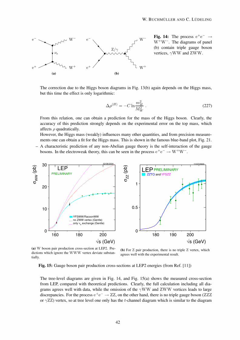
e−

e+

νe

W−

W+

(a)

e−

e+

Z/γ

W−

W+

(b)

Fig. 14: The process e+e− →W+W−. The diagrams of panel(b) contain triple gauge bosonvertices, γWW and ZWW.

The correction due to the Higgs boson diagrams in Fig. 13(b) again depends on the Higgs mass,but this time the effect is only logarithmic:

∆ρ(H) = −C lnm2H

M2W

. (227)

From this relation, one can obtain a prediction for the mass of the Higgs boson. Clearly, theaccuracy of this prediction strongly depends on the experimental error on the top mass, whichaffects ρ quadratically.However, the Higgs mass (weakly) influences many other quantities, and from precision measure-ments one can obtain a fit for the Higgs mass. This is shown in the famous blue-band plot, Fig. 21.

– A characteristic prediction of any non-Abelian gauge theory is the self-interaction of the gaugebosons. In the electroweak theory, this can be seen in the process e+e−→W+W−.

0

10

20

30

160 180 200

√s (GeV)

σ WW

(pb)

YFSWW/RacoonWWno ZWW vertex (Gentle)only νe exchange (Gentle)

LEPPRELIMINARY

02/08/2004

(a) W boson pair production cross-section at LEP2. Pre-dictions which ignore the WWW vertex deviate substan-tially.

708 S. Natale: W and Z pair production at LEP2

0

0.2

0.4

0.6

180 190 200 210

an/Λ2=0.1

an/Λ2=0.2

√s (GeV)

σ WW

γ (pb

)

EEWWG

RacoonWW

LEP PRELIMINARY

13/07/2003

Fig. 4. Combined WWγ cross section as a function of thecenter-of-mass energy. Only L3 and DELPHI results are used

Fig. 5. NC02 diagrams for the production of Z–pair events

The results obtained by the DELPHI, L3 and OPALcollaborations have been combined and they are shown inFig. 4. No statistically significant deviation is observed.

4 ZZ production

At LEP, the Z-pair final state is produced by means oftwo main born level diagrams referred to as NC02 (NeutralCurrent) and shown in Fig. 5. The signal definition for theLEP combination is based on the NC02 set of diagrams,including ISR corrections.

4.1 Selections and results

The experimental investigations of Z-pair production ismade difficult by its rather low cross section, comparedwith competing processes that constitute large and some-times irreducible backgrounds. All 12 visible Z-pair decaycombinations are analysed. In all cases multi-variate tech-niques are used, to enhance the separation power againstthe most important backgrounds, namely W-pair produc-tion. The combination of the Z-pair cross sections as afunction of the center-of-mass energy is shown in Fig. 6.The ratio R, described in the previous section, obtainedusing YFSZZ [11] as theoretical prediction, is R = 0.962±0.055. Good agreement with the Standard Model is ob-served.

5 Conclusions

The amount of data collected by the LEP experimentsin the high energy running period is beeing extensively

0

0.5

1

180 190 200

√s (GeV)

σ ZZ (

pb)

ZZTO and YFSZZLEP PRELIMINARY

11/07/2003

Fig. 6. Combined Z-pair cross sections compared to predictedvalues using the YFSZZ Montecarlo program

analysed and provides a powerful tool to test the StandardModel. In many cases, as for the W-pair cross section, thelevel of accuracy has reached the sensitivity threshold forradiative corrections. Although not yet final, the resultsherein presented are based on the full available statisticsand don’t show deviations from the Standard Model.

Acknowledgements. Let me thank the organisers of EPS03Conference for their professionalism and warm hospitality.I have also to thank my colleagues from the four LEP ex-periments and the members of the LEP Electroweak Work-ing Group for providing the data which were presented in thisreport.

References

1. The ALEPH Collaboration: Nucl. Inst. Meth. A 294, 121(1990)

2. The DELPHI Collaboration: Nucl. Inst. Meth. A 303, 233(1991)

3. The L3 Collaboration: Nucl. Inst. Meth. A 289, 35 (1990)4. The OPAL Collaboration: Nucl. Inst. Meth. A 305, 271

(1991)5. S. Jadach et al.: Phys. Lett. B 417, 326 (1998); Phys. Rev.

D 61, 113010 (2000); UTHEP-00-0101, CERN-TH/2000-337

6. A. Denner et al.: Nucl. Phys. B 587, 67 (2000) hep-ph/0006307

7. The LEP Electroweak Working Group: note in preparation8. N. Cabibbo: Phys. Rev. Lett. 10, 531 (1963); M. Kobayashi

and T. Maskawa: Prog. Theor. Phys. 49, 652 (1973)9. K. Hagiwara et al.: “The 2002 Review of Particle Physics”,

Phys. Rev. D 66, 1 (2002)10. S.L. Glashow: Nucl. Phys. 22, 579 (1961); S. Weinberg:

Phys. Rev. Lett. 19, 1264 (1967); A. Salam: in ElementaryParticle Theory, ed. N. Svartholm, Stockholm, Almquistand Wiksell (1968), 367

11. S. Jadach et al.: Phys. Rev. D 56, 6939 (1997)

(b) For Z pair production, there is no triple Z vertex, whichagrees well with the experimental result.

Fig. 15: Gauge boson pair production cross-sections at LEP2 energies (from Ref. [11])

The tree-level diagrams are given in Fig. 14, and Fig. 15(a) shows the measured cross-sectionfrom LEP, compared with theoretical predictions. Clearly, the full calculation including all dia-grams agrees well with data, while the omission of the γWW and ZWW vertices leads to largediscrepancies. For the process e+e−→ ZZ, on the other hand, there is no triple gauge boson (ZZZor γZZ) vertex, so at tree level one only has the t-channel diagram which is similar to the diagram

42


42

in Fig. 14(a), but with an electron instead of the neutrino. The agreement between theory and datais evident from Fig. 15(b).

5.4.1 Fermi theory

µ−

νµ

e−

νe

Fig. 16: µ decay

The exchange of a W boson with momentum q in a Feynman diagram contributes

a factor of(M2

W − q2)−2

to the amplitude. For low-energy processes like muondecay (see Fig. 16), the momentum transfer is much smaller than the mass ofthe W boson. Hence to good approximation one can ignore q2 and replace thepropagator byM−2

W . This amounts to introducing an effective four-fermion vertex(see Fig. 17),

L effCC = −GF√

2JµCCJ

†CCµ , (228)

where GF is Fermi’s constant,

GF =g2

4√

2M2W

=1

2√

2 v2, (229)

which is inversely proportional to the Higgs vacuum expectation value v2. A four-fermion theory forthe weak interactions was first introduced by Fermi in 1934. Since it is not renormalizable, it cannotbe considered a fundamental theory. However, one can use it as an effective theory at energies smallcompared to the W mass. This is sufficient for many applications in flavour physics, where the energyscale is set by the masses of leptons, kaons and B mesons.

Wq2 M2

W

Fig. 17: W boson exchange can be de-scribed in terms of the Fermi theory, aneffective theory for momentum transferssmall compared to the W mass. The Wpropagator is replaced by a four-fermionvertex ∝ GF.

5.5 SummaryThe electroweak theory is a chiral gauge theory with gauge group SU(2)W × U(1)Y . This symmetry isspontaneously broken down to U(1)em by the Higgs mechanism which generates the gauge boson andHiggs masses, and also all fermion masses, since direct mass terms are forbidden by gauge invariance.

The electroweak theory is extremely well tested experimentally, to the level of 0.1%, which probesloop effects of the non-Abelian gauge theory. The results of a global electroweak fit are shown in Fig. 18.There is one deviation of almost 3σ, all other quantities agree within less than 2σ.

This impressive agreement is only possible because of two properties of the electroweak interac-tions: they can be tested in lepton–lepton collisions, which allow for very precise measurements, andthey can be reliably calculated in perturbation theory. QCD, on the other hand, requires hadronic pro-cesses which are known experimentally with less accuracy and are also theoretically subject to largeruncertainties.

43


43

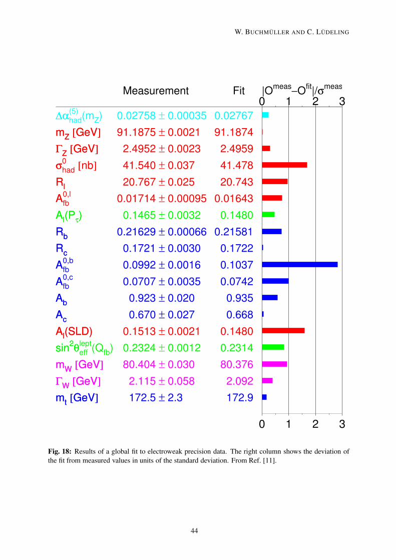
Measurement Fit |Omeas−Ofit|/σmeas

0 1 2 3

0 1 2 3

∆αhad(mZ)∆α(5) 0.02758 ± 0.00035 0.02767mZ [GeV]mZ [GeV] 91.1875 ± 0.0021 91.1874ΓZ [GeV]ΓZ [GeV] 2.4952 ± 0.0023 2.4959σhad [nb]σ0 41.540 ± 0.037 41.478RlRl 20.767 ± 0.025 20.743AfbA0,l 0.01714 ± 0.00095 0.01643Al(Pτ)Al(Pτ) 0.1465 ± 0.0032 0.1480RbRb 0.21629 ± 0.00066 0.21581RcRc 0.1721 ± 0.0030 0.1722AfbA0,b 0.0992 ± 0.0016 0.1037AfbA0,c 0.0707 ± 0.0035 0.0742AbAb 0.923 ± 0.020 0.935AcAc 0.670 ± 0.027 0.668Al(SLD)Al(SLD) 0.1513 ± 0.0021 0.1480sin2θeffsin2θlept(Qfb) 0.2324 ± 0.0012 0.2314mW [GeV]mW [GeV] 80.404 ± 0.030 80.376ΓW [GeV]ΓW [GeV] 2.115 ± 0.058 2.092mt [GeV]mt [GeV] 172.5 ± 2.3 172.9

Fig. 18: Results of a global fit to electroweak precision data. The right column shows the deviation ofthe fit from measured values in units of the standard deviation. From Ref. [11].

44


44

6 The Higgs profileThe only missing building block of the Standard Model is the Higgs boson. Spontaneously brokenelectroweak symmetry, however, is a cornerstone of the Standard Model, and so the discovery of theHiggs boson and the detailed study of its interactions is a topic of prime importance for the LHC and theILC.

The investigation of the Higgs sector can be expected to to give important insight also on physicsbeyond the Standard Model. Since the Higgs is a scalar particle, its mass is subject to quadraticallydivergent quantum corrections, and an enormous ‘fine-tuning’ of the tree-level mass term is needed tokeep the Higgs light (this is usually referred to as the ‘naturalness problem’ of the Higgs sector). Suchconsiderations have motivated various extensions of the Standard Model:

– Supersymmetry retains an elementary scalar Higgs (and actually adds four more), while radiativecorrections with opposite signs from bosons and fermions cancel.

– Technicolour theories model the Higgs as a composite particle of size 1/ΛTC, where ΛTC ∼ 1 TeVis the confinement scale of a new non-Abelian gauge interaction. These theories generically haveproblems with electroweak precision tests and the generation of fermion masses.

– A related idea regards the Higgs as a pseudo-Goldstone boson of some approximate global sym-metry spontaneously broken at an energy scale above the electroweak scale. The Higgs mass isthen related to the explicit breaking of this symmetry.

– In theories with large extra dimensions new degrees of freedom occur, and the Higgs field can beidentified, for instance, as the fifth component of a five-dimensional vector field.

All such ideas can be tested at the LHC and the ILC, since the unitarity of WW scattering implies that theStandard Model Higgs and/or other effects related to electroweak symmetry breaking become manifestat energies below ∼ 1 TeV.

6.1 Higgs couplings and decaySuppose a resonance is found at the LHC with a mass above 114 GeV and zero charge. How can oneestablish that it indeed is the Higgs?

The Higgs boson can be distinguished from other scalar particles as they occur, for instance,in supersymmetric theories, by its special couplings to Standard Model particles. All couplings areproportional to the mass of the particle, since it is generated by the Higgs mechanism. Hence the Higgsdecays dominantly into the heaviest particles kinematically allowed, which are tt or, for a light Higgs,bb and tt pairs. It also has a strong coupling ∝ mH to the longitudinal component of W and Z bosons.The tree-level diagrams are given in Figs. 19(a) and 19(b). In addition, there are important loop-inducedcouplings to massless gluons and photons [see Fig. 19(c)].

The tree-level decay widths in the approximation mH mf ,MW are given by

Γ(H→ ff

)=GFmHm

2f

4π√

2Nc , (230a)

Γ(H→ ZLZL) =1

2Γ(H→WLWL) =

GFm3H

32π√

2. (230b)

The branching fractions of the Higgs into different decay products strongly depend on the Higgs mass, asshown in Fig. 20. For a heavy Higgs, with mH > 2MW , the decay into a pair of W bosons dominates.At the threshold the width increases by two orders of magnitude, and it almost equals the Higgs massat mH ∼ 1 TeV where the Higgs dynamics becomes non-perturbative. For a light Higgs with a massjust above the present experimental limit, mH > 114 GeV, the decay into two photons might be the bestpossible detection channel given the large QCD background for the decay into two gluons at the LHC. It

45


45

H

f

f

∝ mf

(a)

H

WL/ZL

WL/ZL

∝ mH

(b)

H

g/γ

g/γ

(c)

H

H

H

∝ mH

(d)

Fig. 19: Higgs boson decays. Tree-level couplings are proportional to masses, but there also are loop-induced decays into massless particles. The cubic Higgs self-coupling can be probed at the ILC andpossibly at the LHC.

is clearly an experimental challenge to establish the mass dependence of the Higgs couplings, so the truediscovery of the Higgs is likely to take several years of LHC data!

Fig. 20: Left: Higgs branching ratios as function of the Higgs mass. Right: Higgs decay width asfunction of the Higgs mass. It increases by two orders of magnitude at the WW threshold. From Ref. [12].

46


46

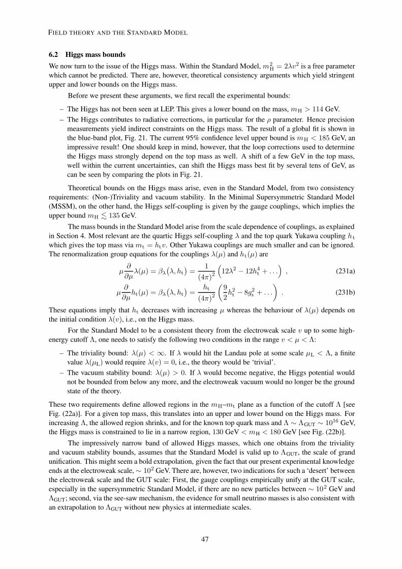
6.2 Higgs mass boundsWe now turn to the issue of the Higgs mass. Within the Standard Model, m2

H = 2λv2 is a free parameterwhich cannot be predicted. There are, however, theoretical consistency arguments which yield stringentupper and lower bounds on the Higgs mass.

Before we present these arguments, we first recall the experimental bounds:

– The Higgs has not been seen at LEP. This gives a lower bound on the mass, mH > 114 GeV.– The Higgs contributes to radiative corrections, in particular for the ρ parameter. Hence precision

measurements yield indirect constraints on the Higgs mass. The result of a global fit is shown inthe blue-band plot, Fig. 21. The current 95% confidence level upper bound is mH < 185 GeV, animpressive result! One should keep in mind, however, that the loop corrections used to determinethe Higgs mass strongly depend on the top mass as well. A shift of a few GeV in the top mass,well within the current uncertainties, can shift the Higgs mass best fit by several tens of GeV, ascan be seen by comparing the plots in Fig. 21.

Theoretical bounds on the Higgs mass arise, even in the Standard Model, from two consistencyrequirements: (Non-)Triviality and vacuum stability. In the Minimal Supersymmetric Standard Model(MSSM), on the other hand, the Higgs self-coupling is given by the gauge couplings, which implies theupper bound mH . 135 GeV.

The mass bounds in the Standard Model arise from the scale dependence of couplings, as explainedin Section 4. Most relevant are the quartic Higgs self-coupling λ and the top quark Yukawa coupling ht

which gives the top mass via mt = htv. Other Yukawa couplings are much smaller and can be ignored.The renormalization group equations for the couplings λ(µ) and ht(µ) are

µ∂

∂µλ(µ) = βλ

(λ, ht

)=

1

(4π)2

(12λ2 − 12h4

t + . . .), (231a)

µ∂

∂µht(µ) = βλ

(λ, ht

)=

ht

(4π)2

(9

2h2

t − 8g2s + . . .

). (231b)

These equations imply that ht decreases with increasing µ whereas the behaviour of λ(µ) depends onthe initial condition λ(v), i.e., on the Higgs mass.

For the Standard Model to be a consistent theory from the electroweak scale v up to some high-energy cutoff Λ, one needs to satisfy the following two conditions in the range v < µ < Λ:

– The triviality bound: λ(µ) < ∞. If λ would hit the Landau pole at some scale µL < Λ, a finitevalue λ(µL) would require λ(v) = 0, i.e., the theory would be ‘trivial’.

– The vacuum stability bound: λ(µ) > 0. If λ would become negative, the Higgs potential wouldnot be bounded from below any more, and the electroweak vacuum would no longer be the groundstate of the theory.

These two requirements define allowed regions in the mH–mt plane as a function of the cutoff Λ [seeFig. (22a)]. For a given top mass, this translates into an upper and lower bound on the Higgs mass. Forincreasing Λ, the allowed region shrinks, and for the known top quark mass and Λ ∼ ΛGUT ∼ 1016 GeV,the Higgs mass is constrained to lie in a narrow region, 130 GeV < mH < 180 GeV [see Fig. (22b)].

The impressively narrow band of allowed Higgs masses, which one obtains from the trivialityand vacuum stability bounds, assumes that the Standard Model is valid up to ΛGUT, the scale of grandunification. This might seem a bold extrapolation, given the fact that our present experimental knowledgeends at the electroweak scale,∼ 102 GeV. There are, however, two indications for such a ‘desert’ betweenthe electroweak scale and the GUT scale: First, the gauge couplings empirically unify at the GUT scale,especially in the supersymmetric Standard Model, if there are no new particles between ∼ 102 GeV andΛGUT; second, via the see-saw mechanism, the evidence for small neutrino masses is also consistent withan extrapolation to ΛGUT without new physics at intermediate scales.

47


47

0

2

4

6

10 102

103

Excluded

mH [GeV]

∆χ2

Preliminary

theory uncertainty

0

2

4

6

102

mH [GeV]∆χ

2

Excluded Preliminary

∆αhad =∆α(5)

0.02761±0.000360.02738±0.00020

theory uncertainty

0

2

4

6

10020 400

mH [GeV]

∆χ2

Excluded Preliminary

∆αhad =∆α(5)

0.02761±0.000360.02747±0.00012Without NuTeV

theory uncertainty

0

1

2

3

4

5

6

10030 500

mH [GeV]

∆χ2

Excluded

∆αhad =∆α(5)

0.02761±0.000360.02749±0.00012incl. low Q2 data

Theory uncertainty

0

1

2

3

4

5

6

10030 300

mH [GeV]

∆χ2

Excluded

∆αhad =∆α(5)

0.02758±0.000350.02749±0.00012incl. low Q2 data

Theory uncertainty

Fig. 21: The blue-band plot showing the constraints on the Higgs mass from precision measurements.The small plots show the same plot from winter conferences of different years: 1997, 2001, 2003 and2005 (left to right). The big plot dates from winter 2006. The best fit and the width of the parabola vary,most notable due to shifts in the top mass and its uncertainty. From Ref. [11].

7 History and outlookFinally, instead of a summary, we shall briefly recall the history of ‘The making of the Standard Model’following a review by S. Weinberg [1]. It is very instructive to look at this process as the interplay ofsome ‘good ideas’ and some ‘misunderstandings’ which often prevented progress for many years.

1. A ‘good idea’ was the quark model, proposed in 1964 independently by Gell-Mann and Zweig.The hypothesis that hadrons are made out of three quarks and antiquarks allowed one to understandtheir quantum numbers and mass spectrum in terms of an approximate SU(3) flavour symmetry,the ‘eightfold way’. Furthermore, the deep-inelastic scattering experiments at SLAC in 1968 couldbe interpreted as elastic scattering of electrons off point-like partons inside the proton, and it wasnatural to identify these partons with quarks.

But were quarks real or just some mathematical entities? Many physicists did not believe in quarks

48


48

(a)

MH

[GeV

/c2]

600

400

500

100

200

300

03 5 7 9 11 13 15 17 19

log10Λ [GeV]

Triviality

EW vacuum is absolute minimum

EWPrecision

Λ

(b)

Fig. 22: Bounds on the Higgs and top mass from triviality and vacuum stability. Panel (a) shows thecombined bounds for different values of Λ (from Ref. [13]). Panel (b) gives the bounds on the Higgsmass for the known top mass (from Ref. [14]).

since no particles with third integer charges were found despite many experimental searches.

2. Another ‘good idea’ was the invention of non-Abelian gauge theories by Yang and Mills in 1954.The local symmetry was the isospin group SU(2), and one hoped to obtain in this way a theory ofstrong interactions with the ρ-mesons as gauge bosons. Only several years later, after the V − Astructure of the weak interactions had been identified, did Bludman, Glashow, Salam and Wardand others develop theories of the weak interactions with intermediate vector bosons.

But all physical applications of non-Abelian gauge theories seemed to require massive vec-tor bosons because no massless ones had been found, neither in strong nor weak interactions.Such mass terms had to be inserted by hand, breaking explicitly the local gauge symmetry andthereby destroying the rationale for introducing non-Abelian local symmetries in the first place.Furthermore, it was realized that non-Abelian gauge theories with mass terms would be non-renormalizable, plagued by the same divergences as the four-fermion theory of weak interactions.

3. A further ‘good idea’ was spontaneous symmetry breaking: There can be symmetries of the La-grangian that are not symmetries of the vacuum. According to the Goldstone theorem there mustbe a massless spinless particle for every spontaneously broken global symmetry. On the otherhand, there is no experimental evidence for any massless scalar with strong or weak interactions.In 1964 Higgs and Englert and Brout found a way to circumvent Goldstone’s theorem: The theo-rem does not apply if the symmetry is a gauge symmetry as in electrodynamics or the non-AbelianYang–Mills theory. Then the Goldstone boson becomes the helicity-zero part of the gauge boson,which thereby acquires a mass.

But again, these new developments were applied to broken symmetries in strong interactions, andin 1967 Weinberg still considered the chiral SU(2)L × SU(2)R symmetry of strong interactionsto be a gauge theory with the ρ and a1 mesons as gauge bosons. In the same year, however, hethen applied the idea of spontaneous symmetry breaking to the weak interactions of the leptonsof the first family, (νL, eL) and eR (he did not believe in quarks!). This led to the gauge group

49


49

SU(2)× U(1), massive W and Z bosons, a massless photon and the Higgs boson!

The next steps on the way to the Standard Model are well known: The proof by ’t Hooft and Veltman thatnon-Abelian gauge theories are renormalizable and the discovery of asymptotic freedom by Gross andWilczek and Politzer. Finally, it was realized that the infrared properties of non-Abelian gauge theorieslead to the confinement of quarks and massless gluons, and the generation of hadron masses. So, by1973 ‘The making of the Standard Model’ was completed!

Since 1973 many important experiments have confirmed that the Standard Model is indeed thecorrect theory of elementary particles:

– 1973: discovery of neutral currents– 1979: discovery of the gluon– 1983: discovery of the W and Z bosons– 1975–2000: discovery of the third family, τ, b, t and ντ

– During the past decade impressive quantitative tests have been performed of the electroweak theoryat LEP, SLC and Tevatron, and of QCD at LEP, HERA and Tevatron.

Today, there are also a number of ‘good ideas’ on the market, which lead beyond the StandardModel. These include grand unification, dynamical symmetry breaking, supersymmetry and string the-ory. Very likely, there are again some ‘misunderstandings’ among theorists, but we can soon hope forclarifications from the results of the LHC.

AcknowledgementsWe would like to thank the participants of the school for stimulating questions and the organizers forarranging an enjoyable and fruitful meeting in Kitzbühel.

AppendixA Vectors, spinors and γ algebraA.1 Metric conventionsOur spacetime metric is mostly minus,

gµν = diag(+,−,−,−) , (A.1)

so timelike vectors vµ have positive norm vµvµ > 0. The coordinate four-vector is xµ = (t, ~x) (with

upper index), and derivatives with respect to xµ are denoted by

∂µ =∂

∂xµ=

(∂

∂t, ~∇). (A.2)

Greek indices µ, ν, ρ, . . . run from 0 to 3, purely spatial vectors are indicated by a vector arrow.

A.2 γ matricesIn four dimensions, the γ matrices are defined by their anticommutators,

γµ, γν = 2gµν, µ = 0, . . . , 3 . (A.3)

In addition, γ0 = γ†0 is Hermitian while the γi = −γ†i are anti-Hermitian, and all γµ are traceless. Thematrix form of the γ matrices is not fixed by the algebra, and there are several common representations,

50


50

like the Dirac and Weyl representations, Eqs. (133) and (58), respectively. However, the followingidentities hold regardless of the representation.

The product of all γ matrices is

γ5 = iγ0γ1γ2γ3 (A.4)

which is Hermitian, squares to one and anticommutes with all γ matrices,γ5, γµ

= 0 . (A.5)

The chiral projectors PL/R are defined as

PL/R =1

2

(1± γ5

), PLPR = PRPL = 0 , P 2

L/R = PL/R . (A.6)

To evaluate Feynman diagrams like for the anomalous magnetic moment, one often needs to con-tract several γ matrices such as

γµγµ = 4 (A.7a)

γµγνγµ = −2γν (A.7b)

γµγνγργµ = 4gνρ (A.7c)

γµγνγργσγµ = −2γσγργν etc. (A.7d)

For a vector vµ we sometimes use the slash /v = γµvµ.

A.3 Dirac, Weyl and Majorana spinorsThe solutions of the Dirac equation in momentum space are fixed by the equations

(/p−m

)u(i)(p) = 0

(/p+m

)v(i)(p) = 0 . (A.8)

Here it is convenient to choose the Weyl representation (58) of the Dirac matrices,

γ0 =

(0

2

2 0

), γi =

(0 σi

−σi 0

), ⇒ γ5 =

(−

2

0

2

).

In this basis, the spinors u(p) and v(p) are given by

us(p) =

(√E

2 + ~p · ~σ ξs√

E

2 − ~p · ~σ ξs

), vs(p) =

( √E

2 + ~p · ~σ ηs

−√E

2 − ~p · ~σ ηs

). (A.9)

Here ξ and η are two-component unit spinors. Choosing the momentum along the z-axis and e.g. ξ =(1, 0)T , the positive-energy spinor becomes

u+ =

√E + pz

0√E − pz

0

, (A.10)

which has spin + 12 along the z-axis. For ξ = (0, 1)T , the spin is reversed, and similar for η and the

negative energy spinors.

51


51

The spinors considered so far are called Dirac spinors: They are restricted only by the Diracequation and have four degrees of freedom (particle and antiparticle, spin up and spin down). There aretwo restricted classes of spinors, Weyl and Majorana spinors, which have only two degrees of freedom.

Weyl or chiral spinors are subject to the constraint

PLψL = ψL or PRψR = ψR (A.11)

and correspond to purely left- or right-handed fermions. In the language of u’s and v’s, chiral spinorscorrespond to sums u± γ5v. Chiral spinors can have a kinetic term, but no usual mass term, since

(ψL) = PLψL = (PLψL)† γ0 = ψ†LPLγ0 = ψLPR (A.12)

and hence

ψL ψL = ψL PRPL︸︷︷︸=0

ψL = 0 . (A.13)

However, there is the possibility of a Majorana mass term via the charge conjugate spinor ψC :

ψC = CψT with the charge conjugation matrix C = iγ0γ2 . (A.14)

ψC is of opposite chirality to ψ, so it can be used to build a bilinear ψCψ for a mass term. However, thisterm violates all symmetries under which ψ is charged, so it is acceptable only for complete singlets, likeright-handed neutrinos.

References[1] S. Weinberg, The making of the Standard Model, Eur. Phys. J. C 34 (2004) 5

[arXiv:hep-ph/0401010].[2] O. Nachtmann, Elementary Particle Physics: Concepts and Phenomena (Springer, Berlin, 1990).[3] M. E. Peskin and D. V. Schroeder, An Introduction to Quantum Field Theory (Addison-Wesley,

Reading, MA, 1995).[4] J. Ellis, lecture given at this School (unpublished).[5] G. Ecker, lecture given at this School, see these proceedings.[6] R. Fleischer, lecture given at this School, see these proceedings.[7] M. Lindner, lecture given at this School (unpublished).[8] S. Weinberg, Gravitation and Cosmology (Wiley, New York, 1972), pp. 61–63.[9] G. ’t Hooft and M. Veltman, Diagrammar, CERN report 73–9 (1973).[10] T. Kinoshita, Nucl. Phys. Proc. Suppl. 157 (2006) 101.[11] LEP Electroweak Working Group, http://lepewwg.web.cern.ch.[12] M. Spira, Fortschr. Phys. 46 (1998) 203 [arXiv:hep-ph/9705337].[13] C. D. Froggatt, Surveys High Energ. Phys. 18 (2003) 77 [arXiv:hep-ph/0307138].[14] C. Quigg, Acta Phys. Polon. B 30 (1999) 2145 [arXiv:hep-ph/9905369].

52


52

Index2→ 2 scattering in φ4 theory, 15

Adjoint spinor, 10Antiparticle, 5Asymptotic freedom, 33Asymptotic states, 14

Bare fields, 30Bare parameters, 30β function, 32

for QCD coupling, 33

Canonical anticommutation relationsfor creation and annihilation operators, 12for spinor fields, 11

Canonical commutation relationsfor p and q, 4for creation and annihilation operators, 6for field operators, 9for raising and lowering operators, 4

Charge operator, 7CKM matrix, 39Compton wavelength, 6Conjugate momentum

for fermions, 11for scalar fields, 9in quantum mechanics, 3

Counterterms, 30Covariant derivative, 19Creation and annihilation operators, 6

Dirac algebra, 10Dirac equation, 10Disconnected diagrams, 14

Electroweak theoryW I and B bosons, 34charged current, 37gauge group, 33isospin and hypercharge currents, 34neutral current, 37quantum numbers, 34

Faddeev–Popov ghosts, 23Fermi constant GF, 43Feynman parameters, 26Feynman propagator, 8

for fermions, 13Feynman rules

for φ4 theory, 14

counterterms, 30for fermions, 16for non-Abelian gauge theories, 23

Field strength, 19Forward–backward asymmetries, 40

γ matrices, 10Dirac representation, 24Weyl representation, 10

Gauge boson self-interaction, 42Gauge conditions, 23Gauge potential

electromagnetic, 18transformation of, 22

Gauge transformation, 18Gordon identity, 25Group generators, 21

Gell-Mann matrices for SU(3), 21Pauli matrices for SU(2), 21

Hamiltonian, 3Harmonic oscillator, 4Heisenberg picture, 4Higgs

mechanism, 36potential, 36

Hilbert spacefor the spinor field, 12of the harmonic oscillator, 4of the scalar field, 6

Lagrange density, 9Lagrange function, 3Lagrangian

non-Abelian gauge field, 22QCD, 22QED, 20

Landé factor, 24Landau pole, 32

Magnetic moment, 24anomalous, 27one-loop correction, 27

Majorana mass, 39Mass dimension, 28Maxwell’s equations, 18Mexican hat potential, 17Momentum operator, 7

Naturalness problem, 45

53


53

Noether current, 17Noether’s theorem, 9

Pauli equation, 25Pauli principle, 13φ4 theory, 13Polarization vector, 23

R ratios, 40Regularization, 27

dimensional, 28Renormalization, 27

constants, 31group equation, 32schemes, 31

Renormalized fields, 30ρ parameter, 41Running coupling, 31

S matrix, 14See-saw mechanism, 39Self-energy

electron, 29photon (vacuum polarisation), 29

Spin operator, 12Spinors, 10Spontaneous symmetry breaking, 38Structure constants, 21SU(n), 20

Θ function, 9Triangle diagrams, 35

u and v spinors, 11Uncertainty relation, 4Unitary gauge, 36

Vacuum, 5Vertex correction, 25

Ward identity, 31Weak mixing angle, 37

54


54

Documents

Field theory and the Standard Model - CERN